Hierarchical Coarse-grained Approach to the Duration-dependent Spreading Dynamics on Complex Networks

Abstract

Various coarse-grained models have been proposed to study the spreading dynamics on complex networks. A microscopic theory is needed to connect the spreading dynamics with individual behaviors. In this letter, we unify the description of different spreading dynamics by decomposing the microscopic dynamics into two basic processes, the aging process and the contact process. A hierarchical duration coarse-grained (DCG) approach is proposed to study the duration-dependent processes. Applied to the epidemic spreading, such formalism is feasible to reproduce different epidemic models, e.g., the SIS and the SIR models, and to associate the macroscopic spreading parameters with the microscopic mechanism. The DCG approach enables us to study the steady state of the duration-dependent SIS model. The current hierarchical formalism can also be used to describe the spreading of information and public opinions, or to model a reliability theory on networks.

Introduction.—The epidemics (Moore and Newman, 2000; Pastor-Satorras and Vespignani, 2001a, b; May and Lloyd, 2001; Cai et al., 2016; Hindes and Schwartz, 2016), rumors or information (Goffman and Newill, 1964; Daley and Kendall, 1964; Moreno et al., 2004; Nematzadeh et al., 2014; Gleeson et al., 2016), and public opinions (K. Sznajd-Weron, 2000; Dornic et al., 2001; Krapivsky and Redner, 2003; Fernández-Gracia et al., 2014), etc., usually spread on complex networks with predefined structures. The spreading dynamics is strongly affected by the characteristic of the structural networks (Albert and Barabási, 2002; Barrat et al., 2012). The utilization of the susceptible-infected-susceptible (SIS) and the susceptible-infected-recovered (SIR) models initiated the study of the epidemic spreading on networks (Pastor-Satorras and Vespignani, 2001a; May and Lloyd, 2001). The network structure, known as the degree distribution, affects the epidemic threshold (Chakrabarti et al., 2008; Mieghem et al., 2009; Gómez et al., 2010; Castellano and Pastor-Satorras, 2010; Ferreira et al., 2012; Li et al., 2012; Barrat et al., 2012; Goltsev et al., 2012; Lee et al., 2013; Boguñá et al., 2013; Castellano and Pastor-Satorras, 2017; Parshani et al., 2010; Wei and Wang, 2020), which is an index to determine the epidemic phase transition whether the disease spreads over society. The spreading dynamics is also affected by the microscopic mechanism, namely, the rules of the state change and the transition rates of the basic processes. Currently, a unified spreading model combining both the network structure and microscopic mechanism remains missing. In this Letter, we propose a unified formalism to describe the spreading dynamics on the network with general microscopic mechanism.

For the Markovian spreading models with constant transition rates, serial mean-field theories have been proposed to describe the spreading dynamics with neglecting the correlation between nodes (Dorogovtsev et al., 2008; Castellano et al., 2009; Pastor-Satorras et al., 2015). For instance, the epidemic threshold of the standard SIS on networks was obtained via the heterogeneous-mean-field approach with the degree distribution (Pastor-Satorras and Vespignani, 2001a, b; May and Lloyd, 2001; Barrat et al., 2012), and was later refined via the quenched-mean-field approach by considering the details of the network topology (Chakrabarti et al., 2008; Mieghem et al., 2009; Castellano and Pastor-Satorras, 2010; Gómez et al., 2010; Ferreira et al., 2012). For a real-world epidemic, the transmissibility varies in different disease stages (Hoppensteadt, 1974; Feng et al., 2007; Magal et al., 2010; Liu et al., 2015; Wang et al., 2016; Mieghem and van de Bovenkamp, 2013; Cator et al., 2013; Yang et al., 2016; Chen et al., 2018; Mieghem and Liu, 2019; de Arruda et al., 2020; Starnini et al., 2017). Namely, the infection rate relies on the infection duration. Such non-Markovian property was proposed to dramatically affect the spreading dynamics and alter the epidemic threshold (Mieghem and van de Bovenkamp, 2013; Cator et al., 2013; Yang et al., 2016; Chen et al., 2018; Mieghem and Liu, 2019; de Arruda et al., 2020). Here we extend the mean-field theories to the duration-dependent spreading models by introducing the probability density function (PDF) of the duration with the varied transition rates adopted from the reliability theory (Rausand and Høyland, 2004; 200, 2006; Rocchi, 2017). In our formalism, the spreading dynamics are decomposed into two basic processes, the aging process describing the self-evolution of one node (single-body process), and the contact process describing the state change of two connected nodes (two-body process). The two processes are modeled here as a continuous-time stochastic process among a set of discrete states.

Inspired by the coarse-grained approaches of the complex networks (Gfeller and Rios, 2007, 2008; Chen et al., 2010; Shen et al., 2011), the duration-dependent spreading models are presented in three hierarchies, the microscopic, the mesoscopic, and the macroscopic models. In the microscopic model, we derive the basic equations of the PDF of each node with neglecting the correlation between nodes. In the microscopic model, a duration coarse-grained (DCG) approach is proposed to obtain the coarse-grained PDF of the ensemble with the same degree, and gives a refined spreading rate for the duration-dependent SIS model. The microscopic and the mesoscopic models extend the quenched and the heterogeneous mean-field approaches to the duration-dependent spreading models, respectively. The macroscopic model describes the spreading dynamics by assuming the identical PDF of all nodes, and recovers to the compartmental epidemic model (W.O. Kermack, 1927; Brauer et al., 2019; Du and Sun, 2020). The macroscopic model is quantitatively applicable for a homogeneous network with a narrow degree distribution, but gives qualitative prediction about the spreading dynamics.

Two basic processes.—We consider an undirected network with $N_{T}$ nodes represented by an adjacency matrix $A_{lm}$. The node state is picked from the state set $i\in\{0,1,2,...\}$. The state evolution is governed by two basic processes, the aging process and the contact process, as shown in Fig. 1(a) and (b), respectively.

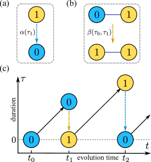
Figure 1: (Color online) Diagrams of the two basic processes. (a) The aging process $1\overset{\alpha(\tau_{1})}{\longrightarrow}0$ describes the recovery of an infected node. (b) The contact process $0+1\overset{\beta(\tau_{0},\tau_{1})}{\longrightarrow}1+1$ describes the infection of a susceptible node raised by an linked node. (c) The evolution of one node, where $\tau$ and $t$ are the duration on one state and the evolution time, respectively.

The aging process describes the state change $i\overset{\alpha_{i^{\prime},i}}{\longrightarrow}i^{\prime}$ of one single node. The transition rate $\alpha_{i^{\prime},i}(\tau_{i})$ generally relates to its duration $\tau_{i}$ on the state $i$ (200, 2006). The maximum entropy principle can be used to estimate the most probable transition rate (Du et al., 2020; Du and Sun, 2020), when limited information, e.g., the mean infection time, is known about the process.

The contact process describes the correlated state change $i+j\overset{\beta_{i^{\prime}j^{\prime},ij}}{\longrightarrow}i^{\prime}+j^{\prime}$ of two linked nodes. The transition rate $\beta_{i^{\prime}j^{\prime},ij}(\tau_{i},\tau_{j})$ relates to the duration $\tau_{i}$ and $\tau_{j}$ of the two nodes in the states $i$ and $j$. Different patterns exist for the contact process, e.g., the exchange process $i+j\overset{\beta_{ji,ij}}{\longrightarrow}j+i$ and the infection process $i+j\overset{\beta_{jj,ij}}{\longrightarrow}j+j$.

A majority of spreading models can be constructed with the two basic processes above. For example, two states $0$ and $1$ are the susceptible and the infected states in the SIS model. The basic processes are an aging process $1\overset{\alpha(\tau_{1})}{\longrightarrow}0$ with the recovery rate $\alpha(\tau_{1})$, and a contact process $0+1\overset{\beta(\tau_{0},\tau_{1})}{\longrightarrow}1+1$ with the infection rate $\beta(\tau_{0},\tau_{1})$. The duration-dependent infection rate $\beta(\tau_{0},\tau_{1})$ reflects the change of both the vulnerability of the susceptible state and the transmissibility of the infected state with their duration. The typical evolution of one node is shown in Fig. 1(c). At the initial time $t=t_{0}$, the node stays in the state $0$ with zero duration $\tau=0$. Its state changes accompanied with resetting the duration at time $t_{1}$ and $t_{2}$ due to the contact and the aging processes. In the typical model of rumor spreading (Daley and Kendall, 1964; Moreno et al., 2004), three states $0$, $1$ and $2$ are the ignorant, spreading, and stifling states, the change of which is governed by three basic processes $0+1\overset{\beta_{1}(\tau_{0},\tau_{1})}{\longrightarrow}1+1$, $1+1\overset{\beta_{2}(\tau_{1},\tau_{1})}{\longrightarrow}2+1$, and $1+2\overset{\beta_{3}(\tau_{1},\tau_{2})}{\longrightarrow}2+2$. The transition rates generally depend on the duration, but such duration-dependent effects have seldom been considered in the current studies.

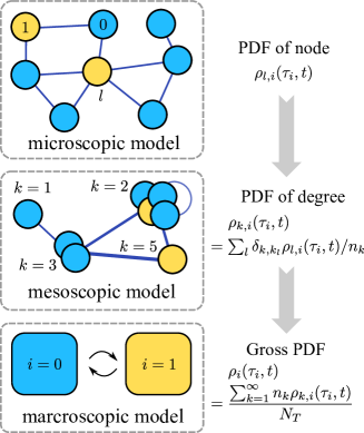
Figure 2: (Color online) Hierarchy of the microscopic, the mesoscopic, and the macroscopic models of the spreading dynamics. The information of the duration distribution is recorded by the probability density function $\rho_{l,i}(\tau_{i},t)$, $\rho_{k,i}(\tau_{i},t)$ and $\rho_{i}(\tau_{i},t)$ at different coarse-grained levels.

Duration-dependent spreading models.—The conventional spreading models (Pastor-Satorras and Vespignani, 2001a; Barrat et al., 2012) with only recording the node states are not enough to describe the spreading dynamics with the duration-dependent transition rates. In Fig. 2(a), we introduce the probability density function (PDF) $\rho_{l,i}(\tau_{i},t)$ of the duration for the node $l$ in the microscopic model. The probability of the node $l$ in the state $i$ follows as $P_{l,i}(t)=\int_{0}^{\infty}\rho_{l,i}(\tau_{i},t)d\tau_{i}$. By neglecting the correlation between nodes, the state of the network is described by the PDF $\rho_{l,i}(\tau_{i},t)$. The equation of the PDF reads (see the derivation in supplementary materials (sup, ))

$$\frac{\partial\rho_{l,i}(\tau_{i},t)}{\partial\tau_{i}}+\frac{\partial\rho_{l,i}(\tau_{i},t)}{\partial t}=-\Gamma_{l,i}(\tau_{i},t)\rho_{l,i}(\tau_{i},t).$$ (1)

The total transformation rate for the node $l$ of leaving the state $i$ is $\Gamma_{l,i}(\tau_{i},t)=\sum_{i^{\prime}}\gamma_{l,i^{\prime}i}(\tau_{i},t)$, with the transformation rate $\gamma_{l,i^{\prime}i}(\tau_{i},t)$ from the state $i$ to the state $i^{\prime}$ explicitly as

$$\gamma_{l,i^{\prime}i}=\alpha_{i^{\prime},i}+\sum_{m,j,j^{\prime}}A_{lm}\int_{0}^{\infty}\beta_{i^{\prime}j^{\prime},ij}\rho_{m,j}d\tau_{j}.$$ (2)

The connecting condition for the PDF at the boundary $\tau_{i}=0$ is determined by the flux to the state $i$ as $\rho_{l,i}(0,t)=\Phi_{l,i}(t)=\sum_{i^{\prime}}\phi_{l,ii^{\prime}}(t),$ where $\phi_{l,ii^{\prime}}(t)=\int_{0}^{\infty}\gamma_{l,ii^{\prime}}(\tau_{i^{\prime}},t)\rho_{l,i^{\prime}}(\tau_{i^{\prime}},t)d\tau_{i^{\prime}}$ is the probability of the node $l$ transforming from the state $i^{\prime}$ to the state $i$ in unit time.

To effectively describe the spreading dynamics without considering the state of each node, we propose a duration coarse-grained (DCG) approach to study the duration-dependent effect with the coarse-grained PDF. In the mesoscopic model, the nodes are sorted into different ensembles with the degree $k$, as shown in Fig 2(b). The states of the network are described by the coarse-grained PDF of the $k$-degree nodes as $\rho_{k,i}(\tau_{i},t)=\sum_{l}\delta_{k,k_{l}}\rho_{l,i}(\tau_{i},t)/n_{k}$ with the population $n_{k}$ of all $k$-degree nodes. The population of the $k$-degree nodes in the state $i$ follows as $n_{k,i}(t)=n_{k}\int_{0}^{\infty}\rho_{k,i}(\tau_{i},t)d\tau_{i}$. The PDFs of the nodes with the same degree are assumed identical $\rho_{l,i}(\tau_{i},t)=\rho_{k_{l},i}(\tau_{i},t)$, and the transformation rate of a node only relies on its degree as $\gamma_{k_{l},i^{\prime}i}(\tau_{i},t)$. The equation of the coarse-grained PDF of the $k$-degree nodes is obtained from Eq. (1) as

$$\frac{\partial\rho_{k,i}(\tau_{i},t)}{\partial\tau_{i}}+\frac{\partial\rho_{k,i}(\tau_{i},t)}{\partial t}=-\Gamma_{k,i}(\tau_{i},t)\rho_{k,i}(\tau_{i},t).$$ (3)

The total transformation rate is $\Gamma_{k,i}(\tau_{i},t)=\sum_{i^{\prime}}\gamma_{k,i^{\prime}i}(\tau_{i},t)$, and the transformation rate $\gamma_{k,i^{\prime}i}(\tau_{i},t)$ is simplified as

$$\gamma_{k,i^{\prime}i}=\alpha_{i^{\prime},i}+k\sum_{j,j^{\prime}}\sum_{k^{\prime}=1}^{\infty}P(k^{\prime}|k)\int_{0}^{\infty}\beta_{i^{\prime}j^{\prime},ij}\rho_{k^{\prime},j}d\tau_{j},$$ (4)

where the degree correlation $P(k^{\prime}|k)$ describes the degree distribution of a neighbor of a $k$-degree node, and is determined by the adjacency matrix $A_{lm}$ as $P(k^{\prime}|k)=\sum_{l,m}\delta_{k,k_{l}}\delta_{k^{\prime},k_{m}}A_{lm}/(kn_{k})$ (sup, ). The connecting condition for the coarse-grained PDF is $\rho_{k,i}(0,t)=\Phi_{k,i}(t)=\sum_{i^{\prime}}\phi_{k,ii^{\prime}}(t),$ where $\phi_{k,ii^{\prime}}(t)=\int_{0}^{\infty}\gamma_{k,ii^{\prime}}(\tau_{i^{\prime}},t)\rho_{k,i^{\prime}}(\tau_{i^{\prime}},t)d\tau_{i^{\prime}}$ is the flux of one $k$-degree node transforming from the state $i^{\prime}$ to the state $i$. An example with explicit equations of PDFs in the duration-dependent SIS model can be found in the supplementary materials (sup, ) or in Ref. (Yang et al., 2016).

At the macroscopic level, a further coarse-grained procedure introduces the gross PDF $\rho_{i}(\tau_{i},t)=[\sum_{k=1}^{\infty}n_{k}\rho_{k,i}(\tau_{i},t)]/N_{T}$ of all nodes to simplify the spreading dynamics, as shown in Fig. 2(c). The dynamics is then regarded to be homogeneous for all nodes independent of the degree. The population of the nodes in the state $i$ follows as $N_{i}(t)=N_{T}\int_{0}^{\infty}\rho_{i}(\tau_{i},t)d\tau_{i}$. This approximation is suitable for the homogeneous network with similar degrees for all nodes. The equation of the gross PDF is obtained from Eq. (3) as

$$\frac{\partial\rho_{i}(\tau_{i},t)}{\partial\tau_{i}}+\frac{\partial\rho_{i}(\tau_{i},t)}{\partial t}=-\Gamma_{i}(\tau_{i},t)\rho_{i}(\tau_{i},t).$$ (5)

The total transformation rate is $\Gamma_{i}(\tau_{i},t)=\sum_{i^{\prime}}\gamma_{i^{\prime}i}(\tau_{i},t)$, with the transformation rate $\gamma_{i^{\prime}i}(\tau_{i},t)$ explicitly as

$$\gamma_{i^{\prime}i}=\alpha_{i^{\prime},i}+\left\langle k\right\rangle\sum_{j,j^{\prime}}\int_{0}^{\infty}\beta_{i^{\prime}j^{\prime},ij}\rho_{j}d\tau_{j}.$$ (6)

The effect of the network structure on the spreading dynamics is reflected by the average degree $\left\langle k\right\rangle=\sum_{k=1}^{\infty}kP(k)$. The connecting condition for the gross PDF is $\rho_{i}(0,t)=\Phi_{i}(t)=\sum_{i^{\prime}}\phi_{ii^{\prime}}(t)$ with the gross flux $\phi_{ii^{\prime}}(t)=\int_{0}^{\infty}\gamma_{ii^{\prime}}(\tau_{i^{\prime}},t)\rho_{i^{\prime}}(\tau_{i^{\prime}},t)d\tau_{i^{\prime}}$. Details of the coarse-grained procedures are shown in the supplementary materials (sup, ).

Our spreading models can be widely used to describe different problems with different meanings of the states and the nodes. For example, the node states describe disease of individuals in an epidemic model (Pastor-Satorras and Vespignani, 2001a), or performance of components in a reliability model (Rocchi, 2017). The transformation rates and the connecting conditions are given accordingly from the specific microscopic mechanism. For the constant transition rates, our models retain the conventional models describing the spreading dynamics with the probabilities $P_{l,i}(t)$ or the populations $n_{k,i}(t)$ and $N_{i}(t)$. The detailed derivation is given in the supplementary materials (sup, ).

	SIS model	SIR model
Node states	$0,1$	$0,1,2$
Rules	$1\overset{\alpha(\tau_{1})}{\longrightarrow}0$ $0+1\overset{\beta(\tau_{0},\tau_{1})}{\longrightarrow}1+1$	$1\overset{\alpha(\tau_{1})}{\longrightarrow}2$ $0+1\overset{\beta(\tau_{0},\tau_{1})}{\longrightarrow}1+1$
Transformation rates	$\Gamma_{k,1}(\tau_{1},t)=\alpha(\tau_{1})$
	$\Gamma_{k,0}(\tau_{0},t)=k\int_{0}^{\infty}\beta(\tau_{0},\tau_{1})\sum_{k^{\prime}=1}^{\infty}P(k^{\prime}|k)\rho_{k^{\prime},1}(\tau_{1},t)d\tau_{1}$
Fluxes	$\Phi_{k,0}(t)=\int_{0}^{\infty}\alpha(\tau_{1})\rho_{k,1}(\tau_{1},t)d\tau_{1}$ $\Phi_{k,1}(t)=\int_{0}^{\infty}\Gamma_{k,0}(\tau_{0},t)\rho_{k,0}(\tau_{0},t)d\tau_{0}$	$\Phi_{k,2}(t)=\int_{0}^{\infty}\alpha(\tau_{1})\rho_{k,1}(\tau_{1},t)d\tau_{1}$ $\Phi_{k,1}(t)=\int_{0}^{\infty}\Gamma_{k,0}(\tau_{0},t)\rho_{k,0}(\tau_{0},t)d\tau_{0}$
Connecting conditions	$\rho_{k,0}(0,t)=\Phi_{k,0}(t)$ $\rho_{k,1}(0,t)=\Phi_{k,1}(t)$	$\rho_{k,0}(0,t)=0$ $\rho_{k,1}(0,t)=\Phi_{k,1}(t)$ $\rho_{k,2}(0,t)=\Phi_{k,2}(t)$

Table 1: The dictionary for constructing the duration-dependent SIS and SIR model.

As follows, we apply our spreading models to the epidemic spreading. In Tab. 1, we list the dictionary for constructing the duration-dependent SIS and SIR models with the transformation rates, the fluxes and the connecting conditions in the mesoscopic model. The two models are uniformly described by the same partial differential equations with different coupling forms of the connecting conditions.

The macroscopic model of spreading dynamics recovers to the standard compartmental SIS model (W.O. Kermack, 1927; Bailey, 1975; Brauer et al., 2019) with the constant recovery $\alpha$ and infection rate $\beta$, where the susceptible and the infected populations satisfy $\dot{N}_{0}(t)=\alpha N_{1}(t)-\beta\left\langle k\right\rangle N_{0}(t)N_{1}(t)/N_{T}$ and $N_{1}(t)=N_{T}-N_{0}(t)$. In Ref. (Du et al., 2020), the effect of the duration-dependent recovery rate $\alpha(\tau_{1})$ has been studied in an extended compartmental model with the integro-differential equations. In the supplementary materials (sup, ), we derive both the standard and the extended compartmental model from the macroscopic model.

SIS model in a network.—The current DCG approach is applied to solve the spreading dynamics of the duration-dependent SIS model on an uncorrelated network with the degree correlation $P(k^{\prime}|k)=k^{\prime}P(k^{\prime})/\left\langle k\right\rangle$ (Barrat et al., 2012). The DCG approach enables us to obtain the steady state with arbitrary duration-dependent recovery and infection rates by solving a self-consistent equation.

In the duration-dependent SIS model, the DDFs $\rho_{k,0}(\tau_{0},t)$ and $\rho_{k,1}(\tau_{1},t)$ obey Eq. (3) with the transformation rates and the connecting conditions listed in Tab. 1. The epidemic spreading is typically assessed by the fraction $r_{1}(t)=\left(\sum_{k=1}^{\infty}n_{k,1}(t)\right)/\left(\sum_{k=1}^{\infty}n_{k}\right)$ of the infected nodes. For the infection rate $\beta(\tau_{0},\tau_{1})$, the dependence on the susceptible and the infection duration describes the vulnerability of a susceptible node and the transmissibility of an infected node, respectively. For simplicity, we assume the vulnerability of the susceptible node does not rely on the susceptible duration (sel, ). Namely, the spreading dynamics is independent of the susceptible duration $\tau_{0}$, and the infection rate only depends on the infection duration $\tau_{1}$ as $\beta(\tau_{0},\tau_{1})=\beta(\tau_{1})$.

On the uncorrelated network, the transformation rate of the contact process is simplified as $\Gamma_{k,0}(t)=k\Theta(t)$ with

$$\Theta(t)=\sum_{k=1}^{\infty}\frac{kP(k)}{\left\langle k\right\rangle}\int_{0}^{\infty}\beta(\tau_{1})\rho_{k,1}(\tau_{1},t)d\tau_{1}.$$ (7)

For the steady state $\partial\rho_{k,i}(\tau_{i},t)/\partial t=0$ of Eq. (3), the DDFs of the steady state are solved as

$$\rho_{k,0}(\tau_{0})=\Phi_{k}\exp[-k\Theta\tau_{0}],$$ (8)

and

$$\rho_{k,1}(\tau_{1})=\Phi_{k}\exp[-\int_{0}^{\tau_{1}}\alpha(\tau)d\tau].$$ (9)

where $\Phi_{k}=n_{k}k\Theta/(1+k\Theta\bar{\tau}_{1})$ is the steady-state flux with the average infection duration $\bar{\tau}_{1}=\int_{0}^{\infty}\exp[-\int_{0}^{\tau_{1}}\alpha(\tau)d\tau]d\tau_{1}$, i.e., the average time to recover from the disease. It follows from Eq. (7) that

$$\Theta=\frac{\Upsilon\Theta}{\left\langle k\right\rangle}\sum_{k=1}^{\infty}\frac{k^{2}P(k)}{1+k\Theta\bar{\tau}_{1}},$$ (10)

which is the self-consistent equation for the quantity $\Theta$ of the steady state. Here, $\Upsilon$ is the refined spreading rate for the duration-dependent SIS model as

$$\Upsilon=\int_{0}^{\infty}\beta(\tau_{1})\exp[-\int_{0}^{\tau_{1}}\alpha(\tau)d\tau]d\tau_{1}.$$ (11)

The steady-state fraction of the infected nodes is

$$r_{1}=\sum_{k=1}^{\infty}\frac{k\Theta\bar{\tau}_{1}}{1+k\Theta\bar{\tau}_{1}}P(k),$$ (12)

which is determined by the refined spreading rate $\Upsilon$ via the quantity $\Theta$ and the average infection duration $\bar{\tau}_{1}$ (sin, ). The effect of network structure is explicitly reflected via the degree distribution $P(k)$. For the constant recovery and infection rates, the refined spreading rate $\Upsilon$ returns to the effective spreading rate $\Upsilon=\beta/\alpha$ used in the duration-independent SIS model (Pastor-Satorras and Vespignani, 2001a).

The existence of the non-zero solution $\Theta$ requires the refined spreading rate $\Upsilon$ to exceed a critical value $\Upsilon_{c}=\left\langle k\right\rangle/\left\langle k^{2}\right\rangle$, which is defined as the epidemic threshold solely determined by the network structure. When the refined spreading rate exceeds the epidemic threshold $\Upsilon>\Upsilon_{c}$, the system reaches the epidemic steady state with non-zero infected nodes. At the situation $\Upsilon<\Upsilon_{c}$, the system reaches the disease-free steady state. A necessary condition to ensure a disease-free steady state is $\left\langle k\right\rangle\leq 1/\Upsilon$, which implies the contacts of people need to be controlled according to the spreading ability of the epidemic.

To validate the current coarse-grained model, we simulate the duration-dependent SIS model in an uncorrelated scale-free network with the continuous-time Monte Carlo method (Mieghem, 2006; Li et al., 2012). Details of the simulation are illustrated in the supplementary materials (sup, ). The uncorrelated scale-free network with $N_{T}=2500$ is generated via the configuration model (Catanzaro et al., 2005). The degree sequence $\{k_{l}\}$ is generated according to the degree distribution $P(k)=c/k^{3},$ where $k$ ranges from the minimal degree $k_{\mathrm{min}}=10$ to the maximal degree $k_{\mathrm{max}}=50$ with the normalized constant $c=1/(\sum_{k^{\prime}=k_{\mathrm{min}}}^{k_{\mathrm{max}}}1/k^{\prime 3})$ of the degree distribution. The minimal degree $k_{\mathrm{min}}$ is chosen not so small to avoid large fluctuations of the infected neighbors for low-degree nodes, since the mean-field approach assumes the static PDF for the steady state without considering the fluctuations. The maximal degree $k_{\mathrm{max}}$ fulfills the condition $k_{\mathrm{max}}\leq\sqrt{N_{T}}$ to ensure an uncorrelated network (Catanzaro et al., 2005). All nodes are randomly linked respecting the assigned degrees without multiple and self-connection.

We carry out the simulation with the Weibull distribution of the recovery and the infection time obeying $\psi_{R}(\tau_{I})=a_{\alpha}/b_{\alpha}(\tau_{I}/b_{\alpha})^{a_{\alpha}-1}\exp[-(\tau_{I}/b_{\alpha})^{a_{\alpha}}]$ and $\psi_{I}(T_{I})=a_{\beta}/b_{\beta}(T_{I}/b_{\beta})^{a_{\beta}-1}\exp[-(T_{I}/b_{\beta})^{a_{\beta}}]$, with the corresponding transition rates $\alpha(\tau)=a_{\alpha}/b_{\alpha}(\tau/b_{\alpha})^{a_{\alpha}-1}$ and $\beta(\tau)=a_{\beta}/b_{\beta}(\tau/b_{\beta})^{a_{\beta}-1}$. In each simulation, the evolution is run for 500,000 events to reach the steady state. The steady-state fraction $r_{1}$ is then obtained as the average with 200,000 events.

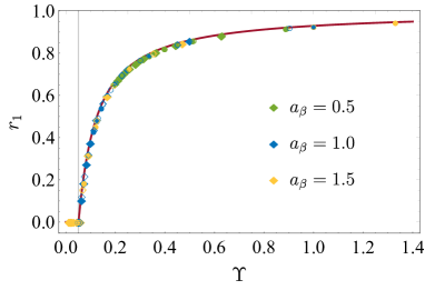
Figure 3: (Color online) The steady-state fraction $r_{1}$ of the infected nodes as the function of the refined spreading rate $\Upsilon$ in the uncorrelated scale-free network. The solid curve is obtained by the DCG approach according to Eq. (12). The markers show the continuous-time Monte Carlo simulation results with Weibull recovery and infection time, where the parameters are set as $a_{\alpha}=1.0$ (filled), $1.5$ (empty), $b_{\alpha}=0.5$ (diamond), $1.0$ (circle) , $a_{\beta}=0.5,\,1.0,\,1.5$ (in different colors), and $b_{\beta}$ ranging from $1.0$ to $10.0$ with the interval $1.0$. The gray vertical line shows the epidemic threshold $\Upsilon_{c}=0.051$ for the current finite-size scale-free network.

In Fig. 3, the steady-state fraction $r_{1}$ of the infected nodes is plotted as the function of the refined spreading rate $\Upsilon$ for the DCG approach (solid curve) and the continuous-time Monte Carlo simulation results (dots). In the simulation, the effects of duration-dependent recovery and the infection rates are considered with different sets of parameters. The agreement between the analytical and the simulation results validates that the steady-state fraction $r_{1}$ can be effectively described with the refined spreading rate $\Upsilon$ by Eq. (11). The curve shows that the existence of the epidemic threshold matches with the theoretical prediction $\Upsilon_{c}=\left\langle k\right\rangle/\left\langle k^{2}\right\rangle=0.051$ (gray grid-line) . The current model shows the availability of the refined spreading rate $\Upsilon$ for justifying the spreading ability of an epidemic.

Conclusion.—In this Letter, we generalize the mean-field theories for the spreading dynamics with duration-dependent mechanism by superseding the probability distribution of states with the PDF of the duration, and show the hierarchical emergence of the widely-used coarse-grained spreading models. The unified formalism enables us to rebuild different epidemic models, e.g., the SIS and the SIR model. Compared to Refs. (Mieghem and van de Bovenkamp, 2013; Cator et al., 2013; Mieghem and Liu, 2019), the refined spreading rate $\Upsilon$ here is suitable for the duration-dependent models as a coarse-grained parameter of the microscopic mechanism details, and also suggests the duration-dependent SIS model can be mapped to the standard one in the meaning of the steady states (Starnini et al., 2017). With the refined spreading rate $\Upsilon$, the epidemic threshold $\Upsilon_{c}=\left\langle k\right\rangle/\left\langle k^{2}\right\rangle$ is applicable for the duration-dependent SIS model to determine the fate of the epidemic spreading.

Limited by the mean-field approach, the current formalism has neglected correlations and fluctuations between nodes, and therefore cannot accurately predict the critical point of the epidemic phase transition, i.e., the epidemic threshold. In the standard SIS model, the correlations and fluctuations affect the epidemic threshold through the mutual reinfection of the high-degree nodes (Goltsev et al., 2012; Boguñá et al., 2013; Lee et al., 2013; Wei and Wang, 2020), and was recently understood through the cumulative merging percolation process (Castellano and Pastor-Satorras, 2020). It is still an open question to describe such correlation effect in a duration-dependent model, which is beyond the scope of the current work and worth for further investigation.