Spectral extended finite element method for band structure calculations in phononic crystals

Abstract

In this paper, we compute the band structure of one- and two-dimensional phononic composites using the extended finite element method (X-FEM) on structured higher-order (spectral) finite element meshes. On using partition-of-unity enrichment in finite element analysis, the X-FEM permits use of structured finite element meshes that do not conform to the geometry of holes and inclusions. This eliminates the need for remeshing in phononic shape optimization and topology optimization studies. In two dimensions, we adopt rational Bézier representation of curved (circular) geometries, and construct suitable material enrichment functions to model two-phase composites. A Bloch-formulation of the elastodynamic phononic eigenproblem is adopted. Efficient computation of weak form integrals with polynomial integrands is realized via the homogeneous numerical integration scheme—a method that uses Euler’s homogeneous function theorem and Stokes’s theorem to reduce integration to the boundary of the domain. Ghost penalty stabilization is used on finite elements that are cut by a hole. Band structure calculations on perforated (circular holes, elliptical holes, and holes defined as a level set) materials as well as on two-phase phononic crystals are presented that affirm the sound accuracy and optimal convergence of the method on structured, higher-order spectral finite element meshes. Several numerical examples are presented to demonstrate the advantages of $p$-refinement made possible by the spectral extended finite element method. In these examples, fourth-order spectral extended finite elements deliver $\mathcal{O}(10^{-8})$ accuracy in frequency calculations with more than thirty-fold fewer degrees-of-freedom when compared to quadratic finite elements.

1 Introduction

The study of wave propagation through macro-scale periodic structures has recently been a topic of significant interest. Research on this topic has been conducted under the umbrella of photonics [1, 2], phononics [3, 4, 5, 6], and metamaterials [7, 8], with the goal of controlling the flow behavior of light, elastic and acoustic waves, heat, or mechanical vibrations in suitably designed materials. Within the scope of phononic structures, a better understanding of periodic oscillations can enable materials capable of wave guiding and redirection [9, 10, 11, 12], wave focusing and amplification [13, 14, 15, 16, 17], and wave absorption and isolation [18, 19, 20]. Additionally, the study of phononic structures has uncovered many interesting phenomena and novel applications, such as ultrasonic tunneling [21], the inverse Doppler effect [22, 23], hypersonic control [24], light/sound interactions [25], and processing of quantum information [26], to name a few.

Historically, numerical efforts in this direction have been driven towards the calculation of the so-called band structure [27] of the periodic system—a graphical representation of the frequency-wavevector pairs that satisfy a certain kind of dispersion relationship for the system. The band structure diagram makes characteristics of band gaps in the periodic structure (such as direction, magnitude, phase, and whether the gap is direct or indirect) readily apparent. Additionally, research areas such as phononic topology optimization [28, 29, 30, 31, 32] and inverse problems in dynamic homogenization [33] depend heavily on the speed, efficiency, and accuracy of the band structure calculating algorithm.

To construct the band structure, the fundamental Bloch-periodic problem solved in the unit phononic cell is: for a given wavevector ($k$-point) in the irreducible Brillouin zone, find the elastodynamic eigenpairs (eigenfrequencies and eigenmodes). Many computational algorithms have been developed to solve this problem. The most common of these approaches is the plane wave expansion (PWE) method [34, 35, 36, 37, 27, 38], which expands both the material properties and the displacement field in a global trigonometric (Fourier) basis. PWE is easy to implement, but the method suffers from slow convergence, especially for cases with sharp material contrasts. Variational methods constitute another broad category of primary phononic computational techniques. These include the Rayleigh quotient [39] and the mixed-variational methods [40, 41, 42, 43]. Of these techniques, the mixed-variational method shows the greatest convergence rates [44] and outperforms the PWE as well [45]. Another major technique is the multiple scattering method [46, 47, 48], which shows good convergence properties but is limited in its applicability to fairly regular material inclusions in the unit cell and is cumbersome to implement. In addition to the aforementioned methods, several secondary acceleration techniques have been developed for phononic computations. These include multipole-multigrid methods [49], multi-scale finite element methods [50], the reduced Bloch mode expansion (RBME) technique [51], and the Bloch Mode Synthesis technique [52]. Further accelerations have been proposed through massive parallelization of the existing algorithms over distributed CPUs and/or GPUs [53].

In this contribution, we use the spectral extended finite element method (X-FEM) [54, 55] to solve the Bloch-periodic elastodynamic eigenproblem over the unit cell. The Galerkin finite element approach proceeds by converting the governing boundary-value problem to an equivalent weak form, then applying a local polynomial approximation (shape function) to trial and test functions over a discretization (mesh) of the Bloch-periodic domain. The finite element method has been previously applied to solve this problem [56, 57, 51], though low-order polynomial approximations typically used within finite elements result in a fine discretization of the domain to accurately capture the waveform solution of the elastodynamic problem. This shortcoming is reduced through the use of higher-order local polynomial approximations, which are enabled by spectral finite elements [58]. With spectral finite elements, solution accuracy improves exponentially in a logarithmic plot with polynomial order ($p$-) refinement of the approximation, as opposed to linear improvement in a logarithmic plot with discretization ($h$-) refinement. This enables a more accurate solution using fewer degrees of freedom. The advantages of spectral finite elements in generating phononic band structures have been recognized [59, 60], though the combination of spectral finite elements and extended finite elements applied to phononic band structure calculations is new to the best knowledge of the authors.

With a conforming mesh of the Bloch-periodic domain, the finite element method can accurately capture solution discontinuities across material boundaries and voids. In comparison, approximations that do not capture discontinuities across boundaries, such as the global Fourier basis used in PWE, suffer from reduced rates of convergence [61]. However, constructing a conforming discretization over an arbitrary domain can be a difficult task that requires advanced mesh generation techniques. Furthermore, iterative design processes, such as those used in phononic topology optimization, can require many meshes to be generated, further increasing the burden of mesh generation. Also, conforming meshes on curved boundaries with higher-order finite elements require a mapping to a parent element with affine geometry. This mapping results in a loss of consistency, which impairs higher order polynomial reproduction on these elements [62, 63, 64]. To eliminate these issues, while maintaining accurate reproduction of domain boundaries, we employ the X-FEM, which can be used to represent boundaries implicitly, through use of enrichment functions [65]. Zhao et al. [66] have demonstrated the promise of the X-FEM using linear elements to construct the band structure diagram for metamaterials. Herein, we extend this idea to incorporate higher-order, spectral shape functions with the X-FEM. Use of the X-FEM with spectral basis functions introduces challenges with respect to boundary representation, interface enrichment, and numerical integration. Chin and Sukumar [55] discuss methods of resolving these challenges, and we apply these improvements to the procedures used in this paper.

The structure of the remainder of this paper follows. In Section 2, we introduce the governing elastodynamic boundary value problem and use Bloch-Floquet theorem to transform the problem to the phononic unit cell, where the strong form and the weak form of the problem are derived. In Section 3, higher order polynomial approximations are introduced as the spectral finite element method. In Section 4, enriched finite element spaces are introduced to capture hole and interface geometry in the unit cell. Also, the finite element equations to solve the phononic unit cell problem are introduced. Section 5 describes how rational Bézier curves and level set functions can be used with the extended finite element method to represent curved geometry. Implementation details, including numerical integration and interface stabilization are discussed in Section 6. In Section 7, several numerical examples in one dimension and two dimensions are discussed which demonstrate the capabilities of the methodology. Finally, in Section 8, we summarize the developments in this paper.

2 Phononic unit cell problem

Consider a two-dimensional periodic composite structure whose unit cell is a parallelogram given by $P\subset\mathbb{R}^{2}$. We define two basis vectors, $\bm{h}_{1}$ and $\bm{h}_{2}$, such that $\bm{x}=\sum_{i=1}^{2}H_{i}\bm{h}_{i}$ for $H_{i}\in[0,1]$ uniquely maps to a point in $P$. An example is illustrated in Fig. 1. The basis vectors can be used to define spatial variation in material properties $\bm{C}(\bm{x})$ (the rank-four modulus tensor) and $\rho(\bm{x})$ (density), since

$$\bm{C}(\bm{x}+n_{i}\bm{h}_{i})=\bm{C}(\bm{x}),\qquad\rho(\bm{x}+n_{i}\bm{h}_{i})=\rho(\bm{x}),$$ (1)

for $n_{i}\in\mathbb{Z}$. We define reciprocal basis vectors

$$\bm{q}_{1}=2\pi\frac{\bm{h}_{2}\times\bm{e}_{3}}{\bm{h}_{1}\cdot\left(\bm{h}_{2}\times\bm{e}_{3}\right)},\qquad\bm{q}_{2}=2\pi\frac{\bm{e}_{3}\times\bm{h}_{1}}{\bm{h}_{2}\cdot\left(\bm{e}_{3}\times\bm{h}_{1}\right)},$$ (2)

where $\bm{e}_{3}$ is a unit vector in the (Cartesian) $z$-direction, such that the property $\bm{h}_{i}\cdot\bm{q}_{j}=2\pi\delta_{ij}$ holds. These reciprocal basis vectors are used to define a wave vector $\bm{k}$ in a periodic composite via $\bm{k}=\sum_{i=1}^{2}Q_{i}\bm{q}_{i}$ where $Q_{i}\in[0,1]$.

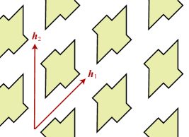
Figure 1: A two-dimensional periodic composite with basis vectors $\bm{h}_{1}$ and $\bm{h}_{2}$.

2.1 Strong formulation

The behavior of waves in solids is governed by the elastodynamic boundary-value problem. Over $\Omega\subseteq P$, the domain of the parallelogram $P$ not including voids, the governing field equations are:

$$\nabla\cdot\bm{\sigma} =\rho\ddot{\bm{u}} \text{(balance of linear momentum)},$$ (3a)

$$\bm{\sigma} =\bm{\sigma}^{T} \text{(balance of angular momentum)},$$ (3b)

$$\bm{\sigma} =\bm{C}:\bm{\varepsilon} \text{(constitutive law)},$$ (3c)

$$\bm{\varepsilon} =\frac{1}{2}\left(\nabla\bm{u}+(\nabla\bm{u})^{T}\right) \text{(small-strain kinematics)},$$ (3d)

where $\bm{\sigma}:=\bm{\sigma}(\bm{x},t)$ is the Cauchy stress tensor, $\rho:=\rho(\bm{x})$ is the scalar density field, $\bm{u}:=\bm{u}(\bm{x},t)$ is the displacement field, and $\bm{\varepsilon}:=\bm{\varepsilon}(\bm{x},t)$ is the strain tensor. We assume plane strain conditions ($\varepsilon_{13}=\varepsilon_{23}=\varepsilon_{33}=0$). Since the problem is time-harmonic with angular frequency $\omega$, the field quantities can be decomposed as follows:

$$\bm{u}(\bm{x},t)=\bm{u}(\bm{x})\exp(-i\omega t),\qquad\bm{\sigma}(\bm{x},t)=\bm{\sigma}(\bm{x})\exp(-i\omega t),\qquad\bm{\varepsilon}(\bm{x},t)=\bm{\varepsilon}(\bm{x})\exp(-i\omega t).$$ (4)

Combining (3) and (4), we recover the eigenproblem

$$\nabla\cdot(\bm{C}(\bm{x}):\nabla_{s}\bm{u}(\bm{x}))=-\lambda\rho(\bm{x})\bm{u}(\bm{x}),$$ (5)

where $\lambda=\omega^{2}$ is the eigenvalue and $\nabla_{s}(\cdot)$ denotes the symmetric gradient. According to the Bloch-Floquet theorem, the displacement and stress fields across unit cells are related by

$$\bm{u}(\bm{x}+\bm{h}_{i})=\bm{u}(\bm{x})\exp\bigl{(}i\bm{k}\cdot\bm{h}_{i}\bigr{)},\qquad\bm{\sigma}(\bm{x}+\bm{h}_{i})=\bm{\sigma}(\bm{x})\exp\bigl{(}i\bm{k}\cdot\bm{h}_{i}\bigr{)}.$$ (6)

These relationships can be used to develop Bloch-periodic boundary conditions on the unit cell, which complete the strong form of the unit cell problem. The problem can be stated as follows:

$$\nabla\cdot(\bm{C}(\bm{x}):\nabla_{s}\bm{u}(\bm{x}))+\lambda\rho(\bm{x})\bm{u}(\bm{x}) =0\quad \text{in }\Omega,$$ (7a)

$$\bm{u}(\bm{x}+\bm{h}_{i}) =\bm{u}(\bm{x})\exp(i\bm{k}\cdot\bm{h}_{i})\quad \text{on }\Gamma_{i}\text{ for }i=1,2,$$ (7b)

$$\bm{\sigma}(\bm{x}+\bm{h}_{i})\cdot\bm{n}(\bm{x}+\bm{h}_{i}) =\bm{\sigma}(\bm{x})\cdot\bm{n}(\bm{x})\exp(i\bm{k}\cdot\bm{h}_{i})\quad \text{on }\Gamma_{i}\text{ for }i=1,2,$$ (7c)

where $\bm{n}$ is the unit normal vector pointing outward from the domain, and $\Gamma_{1}$ and $\Gamma_{2}$ are boundary regions that align with basis vectors $\bm{h}_{2}$ and $\bm{h}_{1}$, respectively. These quantities are illustrated in Fig. 2. Additionally, within the unit cell, we assume voids and/or two distinct, linear elastic materials are present. Holes are located in the domain $\Omega_{\text{hole}}$, with boundary $\Gamma_{\text{hole}}$, and the domain of material $m$ is $\Omega_{m}$ for $m=I,II$. The boundary between the two materials is $\Gamma_{\text{mat}}$. With these additional assumptions, we can explicitly state the boundary and interface conditions that must be satisfied within the unit cell:

$$\bm{\sigma}(\bm{x})\cdot\bm{n}(\bm{x}) =\bm{0}\quad \text{on }\Gamma_{\text{hole}},$$ (8a)

$$[[\bm{u}(\bm{x})]] =\bm{0}\quad \text{on }\Gamma_{\text{mat}},$$ (8b)

$$[[\bm{\sigma}(\bm{x})\cdot\bm{n}(\bm{x})]] =\bm{0}\quad \text{on }\Gamma_{\text{mat}},$$ (8c)

where $[[\cdot]]$ is the jump operator that represents the jump in its argument across the interface. These conditions along with (7) constitute the strong form of the Bloch-periodic boundary-value problem.

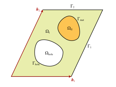
Figure 2: Bloch-periodic boundary-value problem with two distinct linear elastic materials and a hole.

In the developments that follow, we will also consider one-dimensional periodic domains $\Omega=(0,a)$ composed of two, distinct linear elastic materials with properties $(E_{1},\rho_{1})$ and $(E_{2},\rho_{2})$ and an interface at $x=h$. For this problem, the strong form reduces to

$$\begin{gathered}(E(x)u^{\prime}(x))^{\prime}+\lambda\rho(x)u(x)=0\qquad\textrm{ in }\Omega=(0,a),\\ u(a)=\exp(ika)u(0),\qquad E_{2}u^{\prime}(a)=\exp(ika)E_{1}u^{\prime}(0),\\ E_{1}u^{\prime}(h^{-})=E_{2}u^{\prime}(h^{+}),\qquad u(h^{-})=u(h^{+}),\end{gathered}$$ (9)

where $x=h^{-}$ and $x=h^{+}$ are the locations just to the left and right of the interface, respectively.

2.2 Bloch-periodic weak formulation

The strong form of the Bloch-periodic boundary-value problem can be stated equivalently in a weak form which is amenable to computations using the finite element method [67]. Let the trial displacement function $\bm{u}(\bm{x}):\Omega\rightarrow\mathbb{C}$ and test function $\bm{v}(\bm{x}):\Omega\rightarrow\mathbb{C}$ be in $H^{1}(\Omega)$. Following the standard Galerkin procedure, we multiply (7a) by $\bm{v}^{*}(\bm{x})$, the complex conjugate of $\bm{v}(\bm{x})$, and integrate over $\Omega$ to obtain

$$\int_{\Omega}\bm{v}^{*}(\bm{x})\cdot\left[\nabla\cdot(\bm{C}(\bm{x}):\nabla_{s}\bm{u}(\bm{x}))+\lambda\rho(\bm{x})\bm{u}(\bm{x})\right]d\bm{x}=0.$$ (10)

Owing to the discontinuous material density and modulus tensor, the integral can be decomposed to

$$\int_{\Omega_{I}}\bm{v}^{*}(\bm{x})\cdot\left[\nabla\cdot(\bm{C}_{I}:\nabla_{s}\bm{u}(\bm{x}))+\lambda\rho_{I}\bm{u}(\bm{x})\right]d\bm{x}+\int_{\Omega_{II}}\bm{v}^{*}(\bm{x})\cdot\left[\nabla\cdot(\bm{C}_{II}:\nabla_{s}\bm{u}(\bm{x}))+\lambda\rho_{II}\bm{u}(\bm{x})\right]d\bm{x}=0,$$ (11)

where $(\bm{C}_{I},\rho_{I})$ and $(\bm{C}_{II},\rho_{II})$ represent material properties in $\Omega_{I}$ and $\Omega_{II}$, respectively. Integration by parts, using the divergence theorem on the first term of each integral, the symmetry of $\bm{\sigma}(\bm{x})$, and the boundary condition (8a) yields

$$-\int_{\Omega}\nabla_{s}\bm{v}^{*}(\bm{x}):\bm{C}(\bm{x}):\nabla_{s}\bm{u}(\bm{x})\,d\bm{x}+\sum_{i=1}^{2}\int_{\Gamma_{i}}\left[\bm{v}^{*}(\bm{x})\cdot\bm{\sigma}(\bm{x})\cdot\bm{n}(\bm{x})+\bm{v}^{*}(\bm{x}+\bm{h}_{i})\cdot\bm{\sigma}(\bm{x}+\bm{h}_{i})\cdot\bm{n}(\bm{x}+\bm{h}_{i})\right]dS\\ +\int_{\Gamma_{\text{mat}}}[[\bm{v}^{*}(\bm{x})\cdot\bm{\sigma}(\bm{x})\cdot\bm{n}(\bm{x})]]\,dS+\lambda\int_{\Omega}\rho(\bm{x})\bm{v}^{*}(\bm{x})\cdot\bm{u}(\bm{x})\,d\bm{x}=0.$$ (12)

To simplify (12) further, we require $\bm{v}(\bm{x})$ satisfy conditions (8b) and (7b). These conditions give

$$-\int_{\Omega}\nabla_{s}\bm{v}^{*}(\bm{x}):\bm{C}(\bm{x}):\nabla_{s}\bm{u}(\bm{x})\,d\bm{x}+\sum_{i=1}^{2}\int_{\Gamma_{i}}\bm{v}^{*}(\bm{x})\cdot\left[\bm{\sigma}(\bm{x})\cdot\bm{n}(\bm{x})+\exp(-i\bm{k}\cdot\bm{h}_{i})\bm{\sigma}(\bm{x}+\bm{h}_{i})\cdot\bm{n}(\bm{x}+\bm{h}_{i})\right]dS\\ +\lambda\int_{\Omega}\rho(\bm{x})\bm{v}^{*}(\bm{x})\cdot\bm{u}(\bm{x})\,d\bm{x}=0.$$ (13)

Now we apply boundary condition (8c) to arrive at

$$-\int_{\Omega}\nabla_{s}\bm{v}^{*}(\bm{x}):\bm{C}(\bm{x}):\nabla_{s}\bm{u}(\bm{x})\,d\bm{x}+\lambda\int_{\Omega}\rho(\bm{x})\bm{v}^{*}(\bm{x})\cdot\bm{u}(\bm{x})\,d\bm{x}=0.$$ (14)

Stated formally, the weak form is: given $\bm{C}(\bm{x})$, $\rho(\bm{x})$, and $\bm{k}\in\mathbb{R}^{2}$, find $\bm{u}\in\mathcal{S}$ and $\lambda:=\omega^{2}\in\mathbb{R}_{+}$, such that

$$a(\bm{u},\bm{v})+\frac{\gamma_{K}}{h^{2}}j(\bm{u},\bm{v})=\lambda[ b(\bm{u},\bm{v})+\gamma_{M}j(\bm{u},\bm{v})]\quad\forall\bm{v}\in\mathcal{S}$$ (15a)

where

$$a(\bm{u},\bm{v}):=\int_{\Omega}\nabla_{s}\bm{v}^{*}(\bm{x}):\bm{C}(\bm{x}):\nabla_{s}\bm{u}(\bm{x})\,d\bm{x}, \quad b(\bm{u},\bm{v}):=\int_{\Omega}\rho(\bm{x})\bm{v}^{*}(\bm{x})\cdot\bm{u}(\bm{x})\,d\bm{x},$$ (15b)

$$\mathcal{S}:=\Bigl{\{}\;\bm{u}\in\left[H^{1}(\Omega_{I}\cup\Omega_{II})\right]^{2}\;:\;[[\bm{u}]]=\bm{0}\text{ on }\Gamma_{\text{mat}}, \,\,\,\bm{u}(\bm{x}+\bm{h}_{i})=\bm{u}(\bm{x})\exp(i\bm{k}\cdot\bm{h}_{i})\text{ on }\Gamma_{i}\,\,(i=1,2)\;\Bigr{\}}.$$ (15c)

In (15a), the term $j(\bm{u},\bm{v})$ is a ghost penalty [68] stabilization term to improve matrix-conditioning, $\gamma_{K}$ and $\gamma_{M}$ are constants that control the amount of stabilization energy, and $h$ is a characteristic length defined at the element level (see Section 6.2). The ghost penalty term is defined in Section 6.2.

Reduced to one dimension, the weak form is: given $E(\bm{x})$, $\rho(\bm{x})$, and $k\in\mathbb{R}$, find $u\in{\cal S}$ and $\lambda:=\omega^{2}\in\mathbb{R}_{+}$ such that

$$a(v,u)=\lambda\,b(v,u)\quad\forall v\in{\cal S},\quad$$ (16a)

where

$$a(v,u)=\int_{0}^{a}v^{*\prime}(x)E(x)u^{\prime}(x)\,dx,\quad b(v,u)= \int_{0}^{a}\rho(x)v^{*}(x)u(x)\,dx,$$ (16b)

$${\cal S}=\Bigl{\{}\;u\in H^{1}(0,a)\,:\,u(h^{-})=u(h^{+}),\ \ u(a) \ =u(0)\exp(ika)\;\Bigr{\}}.$$ (16c)

3 Spectral finite element method

With X-FEM, geometric features such as holes and material interfaces are not represented by the mesh, so a simple finite element mesh suffices. For applications in solid continua, quadrilateral finite elements are preferred to triangular finite elements, and discretizations aligned with the unit cell basis vectors $\bm{h}_{1}$ and $\bm{h}_{2}$ provide numerous benefits and simplifications as well. From the perspective of the X-FEM, additional advantages include easier implementation for higher-order elements, compatibility with the homogeneous numerical integration (HNI) scheme (requires basis functions that are a linear combination of homogeneous polynomials; see Section 6.1 for details), and simplified computation of the ghost penalty stiffness term introduced in Section 6.2 (over rectangular domains). Accordingly, we restrict ourselves to finite element meshes aligned with the unit cell basis in the subsequent developments.

Consider a tessellation $\mathcal{T}$ of the parallelogram domain $\overline{P}=\overline{\Omega\cup\Omega_{\text{hole}}}$ into a mesh of $M$ elements. The domain of the $e$-th element of the mesh is $\Omega_{e}\subset\mathbb{R}^{2}$. On $\Omega_{e}$, we desire reproduction of $p$-th order polynomials, which is accomplished through a Lagrange interpolation of $(p+1)^{2}$ nodal values. We first develop this interpolant over a parent element, $\Xi=[-1,1]^{2}$, then map it to the domain $\Omega_{e}$. Node locations $\bm{\xi}_{I}\in[-1,1]^{2}$ $\bigl{(}$for $I=1,\dotsc,(p+1)^{2}\bigr{)}$ are chosen as the components of the tensor product of the Gauss-Lobatto points, $\{\xi_{1},\dotsc,\xi_{p+1}\}$ and $\{\eta_{1},\dotsc,\eta_{p+1}\}$. This choice of nodal locations limits oscillation in the interpolation of smooth data (Runge phenomenon). The placement of nodes at the Gauss-Lobatto locations for spectral elements of order $p=2$ to $p=5$ is illustrated in Fig. 3. At each node we define a Lagrange shape function,

$$N_{I(i,j)}(\bm{\xi})=\left(\prod_{\begin{subarray}{c}k=1\\ k\neq i\end{subarray}}^{p+1}\frac{\xi-\xi_{k}}{\xi_{i}-\xi_{k}}\right)\left(\prod_{\begin{subarray}{c}\ell=1\\ \ell\neq j\end{subarray}}^{p+1}\frac{\eta-\eta_{\ell}}{\eta_{j}-\eta_{\ell}}\right)\quad\forall\bm{\xi}\in[-1,1]^{2},$$ (17)

where $I(i,j):\left\{1,2,\dotsc,p+1\right\}^{2}\rightarrow\left\{1,2,\dotsc,(p+1)^{2}\right\}$ uniquely maps components $i$ and $j$ to vector $I$. The shape functions form a basis that uniquely interpolates polynomials up to degree $p$ over $[-1,1]^{2}$. The shape functions are interpolating since the Kronecker delta property, $N_{i}(\bm{\xi}_{j})=\delta_{ij}$, holds.

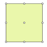
(a)

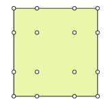
(b)

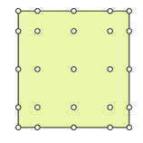
(c)

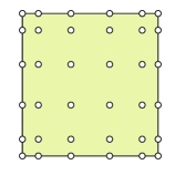
(d)

Figure 3: Gauss-Lobatto nodes for $p$-th order spectral elements. (a) $p=2$, (b) $p=3$, (c) $p=4$, and (d) $p=5$.

Nodes are located in $\Omega_{e}$ through an invertible, affine isoparametric mapping $\bm{x}(\bm{\xi}):\Xi\rightarrow\Omega_{e}$, which is

$$\bm{x}(\bm{\xi})=\bm{H}^{e}\cdot\bm{\xi}+\bm{x}^{e}_{0},$$ (18)

where $\bm{x}^{e}_{0}$ denotes the centroid of the element and the columns of $\bm{H}^{e}$ are the basis vectors of the element domain $\Omega_{e}$ ($\bm{h}^{e}_{1}$ and $\bm{h}^{e}_{2}$). An example isoparametric mapping is shown in Fig. 4. Using the shape functions, we can compute a degree $p$ polynomial approximation of the displacement field over the element:

$$\bm{u}_{e}^{h}(\bm{x})=\sum_{i\in\mathbb{I}_{e}}N_{i}(\bm{x})\bm{u}_{i}\quad\forall\bm{x}\in\Omega_{e},$$ (19)

where $\mathbb{I}_{e}=\left\{1,2,\dotsc,(p+1)^{2}\right\}$ is the index set of nodes in $\Omega_{e}$ and $\bm{u}_{i}:=\bm{u}(\bm{x}_{i})$ are nodal values of displacement. This element-level approximation is utilized in the development of the finite element equations in Section 6.

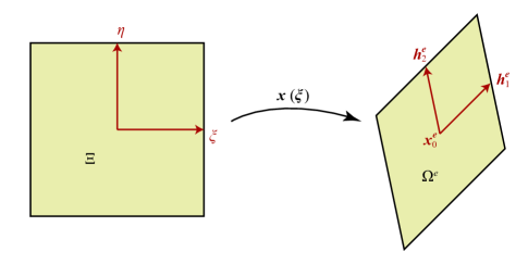
Figure 4: The isoparametric mapping between the parent domain, $\Xi$, and the element domain, $\Omega_{e}$.

4 Extended finite element method

The extended finite element method is an instance of the partition-of-unity finite element method [69], which provides a means to include known solution characteristics in the approximation space. This is accomplished by augmenting the standard finite element space with the product of partition-of-unity functions and enrichment functions. For proofs of convergence with the partition-of-unity finite element method (and, by extension, the X-FEM), we direct the reader to Babuška and Melenk [70] and Babuška et al. [71]. Even though the X-FEM can be used to model a domain that contains both holes and material interfaces, to simplify the exposition, we treat each problem separately. In the sections that follow, we detail the specific enrichment functions used to model holes and material interfaces, respectively.

4.1 Modeling of holes

To capture the effect of holes on the finite element approximation, we construct an enrichment function based on the void geometry as follows [72, 73]:

$$V(\bm{x})=\begin{cases}1&\textrm{if }\bm{x}\notin\Omega_{\text{hole}}\\ 0&\textrm{if }\bm{x}\in\Omega_{\text{hole}}\end{cases}\quad\forall\bm{x}\in\Omega.$$ (20)

An example of an enrichment function for a circular hole is illustrated in Fig. 5(a). For an element in which $\Omega_{e}\cap\Omega_{\text{hole}}\neq\emptyset$, the extended finite element approximation of the displacement field $\bm{u}(\bm{x}):\overline{\Omega}\rightarrow\mathbb{R}^{2}$ restricted to $\overline{\Omega_{e}}\backslash\Omega_{\text{hole}}$ is [72]:

$$\bm{u}_{e}^{h}(\bm{x})=\sum_{i\in\mathbb{I}_{e}}N_{i}(\bm{x})V(\bm{x})\bm{u}_{i},$$ (21)

where $\bm{u}_{i}$ are the nodal displacement degrees of freedom and $N_{i}(\bm{x})$ are the spectral finite element basis functions introduced in (17). Based on the location of $\Omega_{\text{hole}}$ with respect to $\Omega_{e}$, two cases are possible:

1. $\Omega_{e}\cap\Gamma_{\text{hole}}=\emptyset$: the entirety of $\Omega_{e}$ is located in $\Omega_{\text{hole}}$.

2. $\Omega_{e}\cap\Gamma_{\text{hole}}\neq\emptyset$: a portion of $\Omega_{e}$ is located in $\Omega_{\text{hole}}$.

For case 1, the entire element domain is not in the domain of $\bm{u}(\bm{x})$. For case 2, only a portion of the element domain is in the domain of $\bm{u}(\bm{x})$, and the nodal degrees of freedom in this element should only affect the portion of the element not in $\Omega_{\text{hole}}$. This is accomplished through the enrichment function $V(\bm{x})$, which introduces a strong discontinuity at $\Gamma_{\text{hole}}$. Note that if case 1 occurs, there may exist nodes that have no finite element basis function support. An illustration of this scenario is shown in Fig. 5(b). The degrees of freedom (DOFs) at these nodes (the ones that contain crosses in Fig. 5(b)) are removed during the solution procedure. This effectively constrains the displacement of these nodes to zero. This ensures that the stiffness matrix has full rank since there is no strain energy associated with the deformation of these nodes.

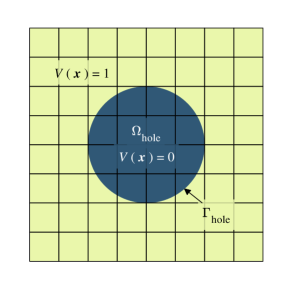
(a)

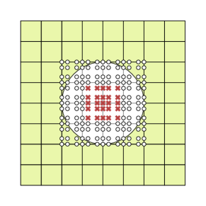
(b)

Figure 5: Modeling a void with the X-FEM. (a) Enrichment function for a circular void, and (b) enriched DOFs (circles) and removed DOFs (crosses) in the vicinity of a void for bilinear finite elements.

4.2 Modeling material interfaces

In an element that intersects the material interface, i.e., $\Omega_{e}\cap\Gamma_{\text{mat}}\neq\emptyset$, the extended finite element approximation takes the form [73]:

$$\bm{u}_{e}^{h}(\bm{x})=\underset{\textrm{standard FE}}{\underbrace{\sum_{i\in\mathbb{I}_{e}}N_{i}(\bm{x})\bm{u}_{i}}}+\underset{\textrm{enriched contribution}}{\underbrace{\sum_{j\in\mathbb{J}_{e}\subseteq\mathbb{I}_{e}}N_{j}(\bm{x})\psi(\bm{x})\bm{a}_{j}}},$$ (22)

where $\psi(\bm{x})$ is the interface enrichment function, $\mathbb{I}_{e}$ is the index set of nodes in $\Omega_{e}$, and $\mathbb{J}_{e}$ is the index set of nodes in $\Omega_{e}$ whose basis function support intersects $\Gamma_{\text{mat}}$. A schematic of a two-phase composite (circular interface) that is modeled using a quadratic finite element mesh is depicted in Fig. 6. In Fig. 6, all the enriched nodes are shown as open circles.

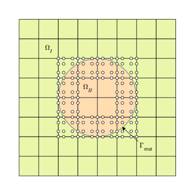
Figure 6: Two-phase composite material. Enriched nodes are marked with an open circle.

To model material interfaces using the X-FEM, the normal strain must admit a jump that satisfies the Hadamard compatibility condition at the interface between two dissimilar isotropic materials [73]. Two additional desirable features of the material interface enrichment function $\psi(\bm{x})$ are:

1. linear, ridge-like variation near the material interface, and

2. zero-value outside enriched elements to avoid the effects of blending elements [74].

If the enrichment function is not affine, the space of polynomial functions that can be reproduced is affected, which ultimately degrades the convergence rate of the method [55]. The modified abs-enrichment introduced by Moës et al. [75] reproduces both these features for linear elements, and a modification to this enrichment function to retain this behavior for higher-order elements with curved interfaces is discussed in Chin and Sukumar [55]. The key features of the enriched element are that it enables independent $p$-th order polynomials to be reproduced on both sides of the material interface and that it enforces $C^{0}$ continuity at the material interface. To define the enrichment function, we first identify two sets of nodes. Over the element tessellation $\mathcal{T}$, let $\mathbb{I}_{\text{enr}}$ be the set consisting of nodes that are enriched, i.e., the nodal basis function support of these nodes intersects $\Gamma_{\text{mat}}$ (nodes marked by circles in Fig. 6). We define $\mathbb{I}_{\text{zero}}\subset\mathbb{I}_{\text{enr}}$ as the set of enriched nodes whose basis of support also includes elements that do not intersect $\Gamma_{\text{mat}}$ (see Fig. 7). The material interface enrichment function is set to zero at these nodes to avoid blending effects in adjacent elements. For a point $\bm{x}\in\Omega_{e}$, we define the function

$$g^{h}(\bm{x})=\sum_{i\in\mathbb{I}_{e}}N_{i}(\bm{x})g_{i},$$ (23)

where $g_{i}$ are nodal values which are set by a two-step process.

1. For nodes $i\in\mathbb{I}_{\text{zero}}$, set $g_{i}=|\varphi_{i}|$, where $\varphi_{i}:=\varphi(\bm{x}_{i})$ are nodal values of the signed distance function to $\Gamma_{\text{mat}}$, and for all other nodes set $g_{i}=0$.

2. Then, for nodes not at the vertices of the element and in $\mathbb{I}_{\text{enr}}\backslash\mathbb{I}_{\text{zero}}$, set $g_{i}=\displaystyle\sum_{j=1}^{4}N^{(p=1)}_{j}(\bm{x}_{i})g_{j}$, where $N^{(p=1)}_{j}(\bm{x})$ are the bilinear finite element shape functions and $g_{j}$ are the element vertex values of $g$ that are set in step 1.

Using (23), we define our material interface enrichment function as

$$\psi(\bm{x})=g^{h}(\bm{x})-|\varphi^{h}(\bm{x})|\quad\forall\bm{x}\in\Omega_{e},$$ (24)

where $\varphi^{h}(\bm{x})=\displaystyle\sum_{i\in\mathbb{I}_{e}}N_{i}(\bm{x})\varphi_{i}$ is the nodal interpolant of the signed distance function. In (24), the second term introduces the ridge with discontinuous derivative at $\Gamma_{\text{mat}}$, whereas the first term shifts the second term to be zero-valued on the appropriate boundaries and approximates a smoothly interpolated bilinear function elsewhere. In Fig. 8, the enrichment function for a circular inclusion over quadratic elements is plotted.

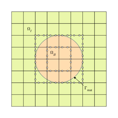
Figure 7: Nodes in $\mathbb{I}_{\text{zero}}$ (marked by open squares) on a $8\times 8$ cubic finite element mesh.

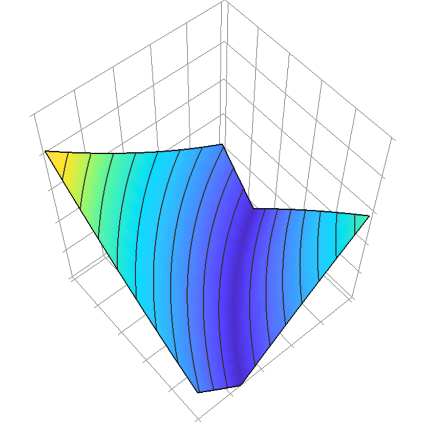
(a) $|\varphi^{h}(\bm{x})|$

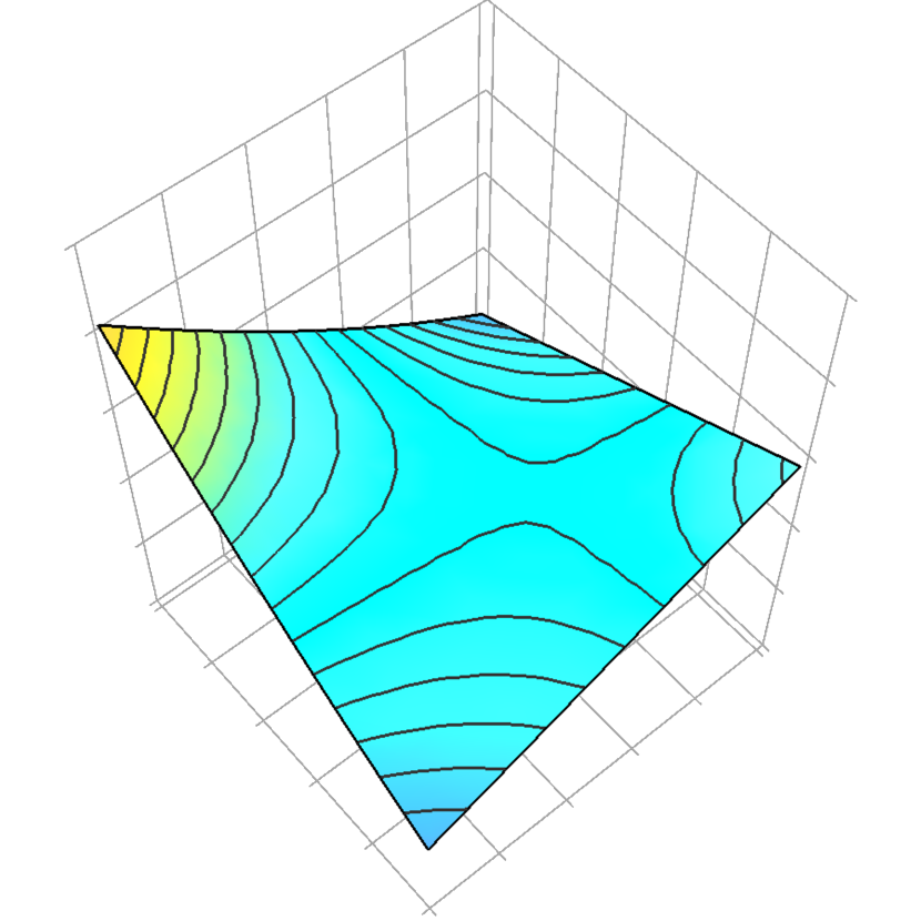
(b) $g(\bm{x})$

(c) $\psi(\bm{x})=g(\bm{x})-|\varphi^{h}(\bm{x})|$

Figure 8: Construction of the enrichment function, $\psi(\bm{x})$, for the material interface problem on a quadratic finite element mesh ($p=2$). The plots are on the element domain $\Omega_{e}=(-0.5,-0.25)^{2}$, with $\varphi(\bm{x})=||\bm{x}||-0.5$.

4.3 Discrete equations

For elements cut by $\Gamma_{\text{hole}}$, we choose (21) to form the trial displacement field $\bm{u}(\bm{x})$ and the test field $\bm{v}(\bm{x})$ in (15a). Then, considering the arbitrariness of nodal variations, we obtain the element level quantities:

$$\bm{K}_{e}=\int_{\Omega_{e}\cap\Omega\backslash\Omega_{\text{hole}}}\big{(}\bm{B}_{u}(\bm{x})\big{)}^{*}\bm{D}(\bm{x})\bm{B}_{u}(\bm{x})\,d\bm{x},\quad\bm{M}_{e}=\int_{\Omega_{e}\cap\Omega\backslash\Omega_{\text{hole}}}\rho(\bm{x})\big{(}\bm{N}_{u}(\bm{x})\big{)}^{*}\bm{N}_{u}(\bm{x})\,d\bm{x},$$ (25)

where $\bm{D}(\bm{x})$ is the piecewise constant two-dimensional linear elastic constitutive matrix and the superscript $(\cdot)^{*}$ denotes the Hermitian of the matrix. In addition, $\bm{N}_{u}(\bm{x})$ is the standard element shape function vector and

$$\bm{B}_{\alpha}(\bm{x})=\begin{bmatrix}\bm{B}_{\alpha}^{1}(\bm{x})&\bm{B}_{\alpha}^{2}(\bm{x})&\dotsc&\bm{B}_{\alpha}^{|\mathbb{L}|}(\bm{x})\end{bmatrix},$$ (26)

where $\alpha=u$, $\mathbb{L}=\mathbb{I}_{e}$ and

$$\bm{B}_{u}^{\ell}(\bm{x})=\begin{bmatrix}N_{\ell,x}(\bm{x})&0\\ 0&N_{\ell,y}(\bm{x})\\ N_{\ell,y}(\bm{x})&N_{\ell,x}(\bm{x})\end{bmatrix}.$$ (27)

Note the Hermitian of element matrices $\bm{B}_{u}(\bm{x})$ and $\bm{N}_{u}(\bm{x})$ is required on account of the Bloch-periodic boundary conditions in (7b).

For elements cut by $\Gamma_{\text{mat}}$, choosing (22) to represent $\bm{u}(\bm{x})$ and $\bm{v}(\bm{x})$ in (15a), and using a standard Galerkin procedure, we obtain the following element quantities:

$$\begin{gathered}\bm{K}_{e}=\bigintsss_{\Omega_{e}}\begin{bmatrix}\big{(}\bm{B}_{u}(\bm{x})\big{)}^{*}\bm{D}(\bm{x})\bm{B}_{u}(\bm{x})&\big{(}\bm{B}_{u}(\bm{x})\big{)}^{*}\bm{D}(\bm{x})\bm{B}_{a}(\bm{x})\\ \big{(}\bm{B}_{a}(\bm{x})\big{)}^{*}\bm{D}(\bm{x})\bm{B}_{u}(\bm{x})&\big{(}\bm{B}_{a}(\bm{x})\big{)}^{*}\bm{D}(\bm{x})\bm{B}_{a}(\bm{x})\\ \end{bmatrix}\,d\bm{x},\\ \bm{M}_{e}=\bigintsss_{\Omega_{e}}\rho(\bm{x})\begin{bmatrix}\big{(}\bm{N}_{u}(\bm{x})\big{)}^{*}\bm{N}_{u}(\bm{x})&\big{(}\bm{N}_{u}(\bm{x})\big{)}^{*}\bm{N}_{a}(\bm{x})\\ \big{(}\bm{N}_{a}(\bm{x})\big{)}^{*}\bm{N}_{u}(\bm{x})&\big{(}\bm{N}_{a}(\bm{x})\big{)}^{*}\bm{N}_{a}(\bm{x})\\ \end{bmatrix}\,d\bm{x},\end{gathered}$$ (28)

where $\bm{B}_{\alpha}(\bm{x})$ for $\alpha=u,a$ is defined in (26) and $\bm{N}_{a}(\bm{x})$ is the element shape function vector for nodes in $\mathbb{J}_{e}$. Referring to (26), for $\alpha=a$ and $\mathbb{L}=\mathbb{J}_{e}$, we define

$$\bm{B}_{a}^{\ell}(\bm{x})=\begin{bmatrix}\left(N_{\ell}(\bm{x})\psi(\bm{x})\right)_{,x}&0\\ 0&\left(N_{\ell}(\bm{x})\psi(\bm{x})\right)_{,y}\\ \left(N_{\ell}(\bm{x})\psi(\bm{x})\right)_{,y}&\left(N_{\ell}(\bm{x})\psi(\bm{x})\right)_{,x}\end{bmatrix}.$$ (29)

For the remaining elements that are not in $\Omega_{\text{hole}}$, no enrichment is required. In these elements, the standard finite element displacement field in (19) is used to approximate $\bm{u}(\bm{x})$ and $\bm{v}(\bm{x})$ in (15a). The resulting element level quantities are:

$$\bm{K}_{e}=\int_{\Omega_{e}}\big{(}\bm{B}_{u}(\bm{x})\big{)}^{*}\bm{D}(\bm{x})\bm{B}_{u}(\bm{x})\,d\bm{x},\quad\bm{M}_{e}=\int_{\Omega_{e}}\rho(\bm{x})\big{(}\bm{N}_{u}(\bm{x})\big{)}^{*}\bm{N}_{u}(\bm{x})\,d\bm{x}.$$ (30)

Assembling element level quantities using the finite element assembly procedure, the generalized eigenproblem, $\bm{Kd}=\lambda\bm{Md}$, is obtained. Element-level integration over elements intersected by holes and material interfaces is conducted using the HNI method, which requires homogeneous integrands. Details of integration using the HNI method are described in Section 6.1. Integration of (30) is accomplished using a tensor-product Gauss-Legendre quadrature rule.

To generate a band structure diagram, the Bloch-periodic weak form is solved for many wave vectors, $\bm{k}$, within the irreducible Brillouin zone of the unit cell. Note the vector of nodal displacements, $\bm{d}$, that satisfies Bloch-periodic boundary conditions given in (15c) is related to the unconstrained vector of nodal displacements, $\hat{\bm{d}}$, via [76]

$$\hat{\bm{d}}:=\bm{R}\bm{d},$$ (31a)

where

$$\bm{R}_{IJ}=\begin{cases}\bm{I}\exp(i\bm{k}\cdot\bm{h}_{i})&\text{if }\bm{d}_{I}\in\mathbb{D}_{i}\\ \bm{I}\delta_{IJ}&\text{otherwise}\end{cases}$$ (31b)

is a $2\times 2$ block in the constraint matrix $\bm{R}$ associated with unconstrained degree of freedom $I$ and constrained degree of freedom $J$, and $\mathbb{D}_{i}$ is the set of nodes located on $\Gamma_{i}$, for $i=1,2$ (see Fig. 2). In (31), $\bm{R}$ is a $\bigl{[}ndof\times 2\bigr{]}\times\bigl{[}(ndof-|\mathbb{D}_{1}|-|\mathbb{D}_{2}|+1)\times 2\bigr{]}$ matrix, where $ndof$ is the number of unconstrained DOFs. The constraint matrix allows the finite element system of equations to be equivalently expressed as

$$\bm{R}^{*}\hat{\bm{K}}\bm{R}\bm{d}=\lambda\bm{R}^{*}\hat{\bm{M}}\bm{R}\bm{d},$$ (32)

where $\hat{\bm{K}}$ and $\hat{\bm{M}}$ are the global stiffness and mass matrices, respectively, with no Bloch-periodic boundary conditions. Thus, $\hat{\bm{K}}$ and $\hat{\bm{M}}$ can be formed once for an extended finite element system of equations, then the matrix $\bm{R}$ can be formed to generate the constrained equations for each $\bm{k}$ in the band structure diagram. While not explored in this paper, secondary acceleration techniques such as RBME [51] and Bloch mode synthesis [52] can also be applied to further reduce the computational burden of computing frequencies at each $k$-point.

For one-dimensional material interface problems, the trial eigenfunction in spectral finite elements is:

$$u^{h}(x) =\sum_{j\in\mathbb{J}}\phi_{j}(x)u_{j}.$$ (33)

where $\mathbb{J}$ is the index set of all nodes in $\Omega$ and $\phi_{j}(x)$ is the spectral finite element basis function associated with node $j$. On choosing $v^{h}=\phi_{i}$ as the test eigenfunction, we obtain the following generalized eigenproblem:

$$\bm{K}\bm{d} =\lambda\bm{M}\bm{d},$$ (34a)

$$\bm{K}_{ij}=\int_{0}^{a}\phi_{i}^{*\prime}E\phi_{j}^{\prime}\,dx ,\quad\bm{M}_{ij}=\int_{0}^{a}\phi_{i}^{*}\rho\phi_{j}\,dx,$$ (34b)

where $\phi_{i}^{*}$ denotes the complex conjugate of $\phi_{i}$.

5 Representation of curved geometries

Two methods of defining curved material and void boundaries are considered in this paper. The first is through an implicit representation of the boundary using level set functions. The second is through quadratic rational Bézier curves, which provide a parametric description of conic boundaries. Explicit, parametric descriptions of the material interface and boundary locations are required to invoke the HNI method. The remainder of this section provides relevant details required to solve a problem using the X-FEM with these representations of curved boundaries.

5.1 Level set representation

In the level set method, isocontours of a $(d+1)$-dimensional function $\varphi(\bm{x})$ are used to track the location of geometric interfaces within a $d$-dimensional domain. We select the level curve $\varphi(\bm{x})=0$ as the interface location. Further, $\varphi(\bm{x})<0$ and $\varphi(\bm{x})>0$ denote regions that lie inside the closed interface and outside the closed interface, respectively. An example of a level set function is the signed distance function, which is used in the material interface enrichment developed in Section 4.2. The level set method simplifies determination of nodal locations with respect to the interface, which simplifies identifying elements that require enrichment in the X-FEM. Consistent with the material interface enrichment in (24), we approximate the level set function at the element level with its nodal interpolant:

$$\varphi^{h}(\bm{x})=\sum_{i\in\mathbb{I}_{e}}N_{i}(\bm{x})\varphi_{i}.$$ (35)

To integrate the weak form integrals in (15a) using the HNI method introduced in Section 6.1, an explicit representation of the interface is required. We employ cubic Hermite functions for this purpose. For the parameter $t\in[0,1]$, a cubic Hermite function is

$$\bm{c}(t,\bm{m})=(2t^{3}-3t^{2}+1)\bm{p}_{0}+(t^{3}-2t^{2}+t)m_{0}\bm{t}_{0}+(-2t^{3}+3t^{2})\bm{p}_{1}+(t^{3}-t^{2})m_{1}\bm{t}_{1},$$ (36)

where $\bm{m}=\left\{m_{0},m_{1}\right\}$, $\bm{p}_{0}$ and $\bm{p}_{1}$ are the endpoints of the curve, and $m_{0}\bm{t}_{0}$ and $m_{1}\bm{t}_{1}$ are the end tangents of the curve at $t=0$ and $t=1$, respectively. The endpoints ($\bm{p}_{0}$ and $\bm{p}_{1}$) and tangent vectors ($\bm{t}_{0}$ and $\bm{t}_{1}$) of the curve are immediately identified by computing $\varphi^{h}(\bm{x})$ and $-\bigl{(}\nabla\varphi^{h}(\bm{x})\bigr{)}^{\perp}$, where $\bigl{(}\nabla\varphi^{h}(\bm{x})\bigr{)}^{\perp}:=\Bigl{[}\bigl{(}\partial\varphi^{h}(\bm{x})\bigr{)}/(\partial y)\ \ -\bigl{(}\partial\varphi^{h}(\bm{x})\bigr{)}/(\partial x)\Bigr{]}^{T}$ is $\nabla\varphi^{h}(\bm{x})$ rotated through $-\pi/2$ radians, at the endpoints. The magnitude of the tangent vector, $m_{0}$ and $m_{1}$, remain to be determined.

The values $m_{0}$ and $m_{1}$ should be selected to approximate the zero isocontour with minimal error. Exact Hermite reconstruction recovers (weakly)

$$F(\bm{m}):=\int_{0}^{1}\left[\varphi^{h}\bigl{(}\bm{c}(t,\bm{m})\bigr{)}\right]^{2}\,dt=0.$$ (37)

Following [55], we choose optimal values of $m_{0}$ and $m_{1}$ by solving

$$\bm{m}^{*}=\operatorname*{arg\,min}_{\bm{m}\in\mathbb{R}^{2}}\ F(\bm{m}).$$ (38)

This numerical optimization problem can be solved using techniques such as Newton’s method or the Broyden-Fletcher-Goldfarb-Shanno (BFGS) algorithm. The BFGS algorithm does not require computing second derivatives of $\varphi^{h}(\bm{x})$, enhancing its appeal in the context of finite elements since second derivatives of shape functions are typically not computed.

If $F(\bm{m}^{*})>0$, then Hermite reconstruction of the isocontour is not exact. Total error over the path is estimated by [55]

$$e(\bm{m}^{*})=\sqrt{\int_{0}^{1}\left(\frac{\varphi^{h}\bigl{(}\bm{c}(t,\bm{m}^{*})\bigr{)}}{\big{|}\big{|}\nabla\varphi^{h}\bigl{(}\bm{c}(t,\bm{m}^{*})\bigr{)}\big{|}\big{|}}\right)^{2}\bigg{|}\bigg{|}\frac{\partial\bm{c}(t,\bm{m}^{*})}{\partial t}\bigg{|}\bigg{|}\,dt}.$$ (39)

The value $e(\bm{m}^{*})$ is compared to a user-defined tolerance, $\epsilon$. If $e(\bm{m}^{*})$ exceeds $\epsilon$, the Hermite curve can be recursively bisected until $e(\bm{m}^{*})<\epsilon$ in all curve segments. This methodology provides a measure of adaptive refinement, optimizing the number and location of Hermite curves needed to accurately trace the implicit curve $\varphi^{h}(\bm{x})=0$.

5.2 Rational Bézier representation

Rational quadratic Bézier curves are capable of exactly representing conic sections such as circles and ellipses. Given Bézier control points $\bm{p}_{0}$, $\bm{p}_{1}$, and $\bm{p}_{2}$ and a coordinate $\bm{x}$, the Bézier curve can be transformed to a level set function by considering its barycentric representation. Note this level set function is not equal to the signed distance function and, therefore, is not a good candidate for use with the material interface enrichment in (24). As described in Farin [77], the linear system of equations,

$$\tau_{0}\bm{p}_{0}+\tau_{1}\bm{p}_{1}+\tau_{2}\bm{p}_{2} =\bm{x},$$

$$\tau_{0}+\tau_{1}+\tau_{2} =1,$$

are solved for parameters $\tau_{0}$, $\tau_{1}$, and $\tau_{2}$. Then, the value of the implicit function is given by

$$\varphi(\bm{x})=\tau_{1}^{2}-4\frac{\tau_{0}\tau_{2}w_{1}^{2}}{w_{0}w_{2}},$$

where $w_{0}$, $w_{1}$, and $w_{2}$ are weights associated with the control points $\bm{p}_{0}$, $\bm{p}_{1}$, and $\bm{p}_{2}$, respectively.

6 Numerical implementation of the X-FEM

6.1 Numerical integration

Discontinuous integrands in (25) and (28) are ill-suited for integration using a tensor-product Gauss rule. To accurately and efficiently integrate the discontinuous weak form integrals, we employ the HNI method. The HNI method traces its origins to Lasserre [78], who used Euler’s homogeneous function theorem to simplify integration over a $d$-dimensional convex polytope to integration over the $(d-1)$-dimensional faces of the polytope. Chin et al. [79] extended Lassere’s approach to nonconvex regions. This section gives a broad overview of the method for two dimensional domains of integration. We refer the reader to Chin and Sukumar [55] for a thorough examination of implementation details.

Let $f(\bm{x})$ be a continuously differentiable, positively homogeneous function of degree $q$. Our objective is to integrate $f(\bm{x})$ over a domain $A\subset\Omega_{e}$, i.e.,

$$I=\int_{A}f(\bm{x})\,d\bm{x}.$$ (40)

The weak form integrands in Section 4.3 are polynomial functions, which can be decomposed into a sum of homogeneous functions. Further, when the domain of integration in enriched elements is split where the integrands are discontinuous, we recover subregions whose boundaries are composed of a combination of affine and curved edges. When $f(\bm{x})$ is a homogeneous polynomial, Euler’s homogeneous function theorem states that

$$qf(\bm{x})=\nabla f(\bm{x})\cdot\bm{x}\quad\forall\bm{x}\in\mathbb{R}^{2}.$$ (41)

For a vector field $\bm{X}:=\bm{X}(\bm{x})$, Stokes’s theorem can be stated as:

$$\int_{A}(\nabla\cdot\bm{X})f(\bm{x})\,d\bm{x}+\int_{A}\nabla f(\bm{x})\cdot\bm{X}\,d\bm{x}=\int_{\partial A}(\bm{X}\cdot\bm{n})f(\bm{x})\,ds,$$ (42)

where $\partial A$ is the boundary of $A$ and $ds$ is differential arc length on $\partial A$. Invoking (41) on homogeneous function $f(\bm{x})$ and choosing $\bm{X}$ as the position vector $\bm{x}$, (42) yields

$$\int_{A}f(\bm{x})\,d\bm{x}=\frac{1}{2+q}\sum_{i=1}^{m}\int_{F_{i}}(\bm{x}\cdot\bm{n}_{i})f(\bm{x})\,ds,$$ (43)

where $\partial A:=\overline{F_{1}\cup F_{2}\cup\ldots\cup F_{m}}$. Equation (43) relates integration of a positively homogeneous function $f(\bm{x})$ over a domain in $\mathbb{R}^{2}$ to integration over the domain’s one-dimensional boundary. We assume that $\partial A=\overline{\partial A_{A}\cup\partial A_{C}}$, where $\partial A_{A}$ is a collection of line segments and $\partial A_{C}$ is a set consisting of parametric curves.

On $\partial A_{A}$, each line segment is the subset of a line given by the equation $\bm{a}\cdot\bm{x}=b$. The unit normal of the line is the normalized gradient of this equation, i.e., $\bm{n}=\bm{a}/||\bm{a}||$. The sign of $\bm{a}$ and $b$ are selected such that $\bm{n}$ points outward from $A$. Substituting into (43), we obtain

$$\int_{F_{i}\subset\partial A_{A}}(\bm{x}\cdot\bm{n}_{i})f(\bm{x})\,ds=\frac{b_{i}}{||\bm{a}_{i}||}\int_{F_{i}\subset\partial A_{A}}f(\bm{x})\,ds.$$ (44)

On $\partial A_{C}$, we consider parametric curves of the form $\bm{c}(t)$, where $t\in[0,1]$ is a parameter such that $\bm{c}(0)$ and $\bm{c}(1)$ give the endpoints of $F_{i}\subset\partial A_{C}$. The curve parameter is chosen such that the boundary is traversed counterclockwise as $t$ increases. We note $\bm{c}(t)$ encompasses many types of curves, including the rational Bézier curves and Hermite spline curves discussed in Section 5. Substituting into (43), we obtain

$$\int_{F_{i}\subset\partial A_{C}}(\bm{x}\cdot\bm{n}_{i})f(\bm{x})\,ds=\int_{0}^{1}\left(\bm{c}_{i}(t)\cdot\bm{n}_{i}\right)f\left(\bm{c}_{i}(t)\right)||\bm{c}^{\prime}_{i}(t)||\,dt,$$ (45)

where $\bm{c}^{\prime}_{i}(t)$ is the derivative with respect to the parameter $t$, i.e., the hodograph of the curve. The normal of $\bm{c}(t)$ is the unit tangent vector rotated counterclockwise through $-\pi/2$ radians. Substituting this into (45) recovers

$$\int_{F_{i}\subset\partial A_{C}}(\bm{x}\cdot\bm{n}_{i})f(\bm{x})\,ds=\int_{0}^{1}\left(\bm{c}_{i}(t)\cdot\bm{c}^{\prime\perp}(t)\right)f\left(\bm{c}_{i}(t)\right)dt.$$ (46)

With (44) and (46), integration over $A$ reduces to one-dimensional integrals over $\partial A$. These integrals are computed using Gauss quadrature. Note if $\bm{c}(t)$ and $f(\bm{x})$ are polynomial, integration is exact with an appropriate quadrature rule.

We use (43), (44), and (46) to develop a cubature rule to apply to the polynomial weak form integrals in Section 4.3. To simplify implementation, we develop a single cubature rule for each element designed to integrate the highest degree polynomial in the integrand. This integration rule is therefore valid on all homogeneous terms of the integrand. On affine edge $F_{j}$, cubature points are Gauss points mapped to $F_{j}$ and cubature weights are selected as $\tilde{w}_{i}b_{j}/||\bm{a}_{j}||$ for $i=1,\ldots,m_{j}$, where $\tilde{w}_{i}$ are Gauss weights of an $m_{j}$-point rule scaled by the length of $F_{j}$. On curved edge $F_{k}$, cubature points are $\bm{x}_{i}=\bm{c}_{k}(t_{i})$, where $t_{i}$ ($i=1,\ldots,m_{k}$) are Gauss points of a $m_{k}$-point rule mapped to the interval $[0,1]$ and cubature weights are $w_{i}=\left(\bm{c}_{k}(t_{i})\cdot\bm{c}_{k}^{\prime\perp}(t_{i})\right)\tilde{w}_{i}$ for $i=1,\ldots,m_{k}$, where $\tilde{w}_{i}$ are Gauss weights of an $m_{k}$-point rule scaled to the interval $[0,1]$.

We decompose a polynomial function, $h(\bm{x})$, into $nh$ $q_{j}$-homogeneous polynomial functions: $f_{j}(\bm{x})$ for $j=1,\dotsc,nh$, such that

$$h(\bm{x})=\sum_{j=1}^{nh}f_{j}(\bm{x}).$$ (47)

Combining the contributions over each boundary edge, the cubature rule is then

$$I=\int_{\Omega_{e}\backslash\Omega_{\text{hole}}}h(\bm{x})\,d\bm{x}\approx\sum_{i=1}^{nq}\sum_{j=1}^{nh}\frac{1}{2+q_{j}}f_{j}(\bm{x}_{i})w_{i},$$ (48)

where $nq$ is the total number of cubature points, $\left\{\bm{x}_{i}\right\}_{i=1}^{nq}$ are the cubature points, and $\left\{w_{i}\right\}_{i=1}^{nq}$ are the cubature weights.

Applying (48) to (25) using a $p$-th order finite element, we obtain

$$\bm{K}_{e} \approx\sum_{i=1}^{nq}\left(\frac{\bm{K}_{e}^{[0]}}{2}+\frac{\bm{K}_{e}^{[1]}(\bm{x}_{i})}{3}+\cdots+\frac{\bm{K}_{e}^{[4p-2]}(\bm{x}_{i})}{4p}\right)w_{i},$$ (49a)

and

$$\bm{M}_{e} \approx\sum_{i=1}^{nq}\left(\frac{\bm{M}_{e}^{[0]}}{2}+\frac{\bm{M}_{e}^{[1]}(\bm{x}_{i})}{3}+\cdots+\frac{\bm{M}_{e}^{[4p]}(\bm{x}_{i})}{4p+2}\right)w_{i},$$ (49b)

where $\bm{K}_{e}^{[q]}$ and $\bm{M}_{e}^{[q]}$ denote the degree-$q$ term in the homogeneous expansions of the integrands in (25). The weak form integrals for an element with interface enrichment can be similarly decomposed to a form amenable to integration using (48).

6.2 Interface stabilization

The extended finite element approximation for holes and material inclusions can induce high condition number in the global finite element stiffness matrix, which can lead to reduced accuracy when solving the algebraic system of linear equations [71]. The reason for poor matrix conditioning is distinct in the hole problem versus the material inclusion problem. For voids, elements where $\Omega_{e}\cap\Omega_{\text{hole}}$ is very large compared to $\Omega_{e}$ cause very small regions of support on some degrees of freedom. These ultimately result in modes of deformation with much lower stiffness and inertia when compared to others, resulting in an ill-conditioned system of linear equations. In the material inclusion problem, conditioning issues arise when $\Omega_{e}\cap\Omega_{I}$ or $\Omega_{e}\cap\Omega_{II}$ is very small compared to $\Omega_{e}$ or when the scaling of the enrichment function substantially differs from the shape functions. A summary of methods to improve conditioning in the X-FEM is discussed in de Prenter et al. [80].

To provide coercivity over the computational domain for the hole problem, we introduce a ghost penalty stabilization energy [68, 81]. The ghost penalty term is designed to eliminate the influence of very small cut elements on the condition number of the stiffness matrix. The term adds additional stiffness and mass contributions to DOFs that have some support in $\Omega_{\text{hole}}$, which minimally changes the finite element solution. We establish the set of elements in $\Omega$ and the set of cut elements as

$$\mathcal{T}_{a}=\Bigl{\{}\;T_{i}\;:\;T_{i}\in\mathcal{T},\,\Omega_{i}\cap\Omega\neq\emptyset\;\Bigr{\}},\quad\mathcal{T}_{c}=\Bigl{\{}\;T_{i}\;:\;T_{i}\in\mathcal{T}_{a},\,\Omega_{i}\cap\Omega\neq\Omega_{i}\;\Bigr{\}},$$

where $T_{i}$ is the $i$-th element in $\mathcal{T}$ with domain $\Omega_{i}$. Additionally, we define a set of edges

$$\mathcal{F}=\Bigl{\{}\;F=T_{i}\cap T_{j}\,:\,T_{i}\in\mathcal{T}_{a},\,T_{j}\in\mathcal{T}_{c}\;\Bigr{\}}$$

for $i,j=1,\ldots,M$. The set of edges $\mathcal{F}$ is demonstrated for two domains in Fig. 9. Following Sticko et al. [82], the supplemental weak form term in (15a) is

$$j(\bm{u},\bm{v})=\sum_{F\in\mathcal{F}}\sum_{k=1}^{p}\frac{h^{2k+1}}{\left(2k+1\right)\left(k!\right)^{2}}\int_{F}\left[\partial^{k}_{\bm{n}}\bm{u}\right]\left[\partial^{k}_{\bm{n}}\bm{v}\right]dS,$$ (50)

where $\bm{n}$ denotes a unit vector normal to $F$, $p$ is the order of the finite element approximation, and $h$ is the average characteristic element length for the two elements connected to $F$. Also appearing in (15a) are the constants $\gamma_{K}:=\beta_{K}(\tilde{\lambda}+2\mu)$ and $\gamma_{M}:=\beta_{K}\rho$, where $\tilde{\lambda}$ and $\mu$ are Lamé parameters for the material, $\rho$ is the density of the material, and $\beta_{K}$ and $\beta_{M}$ are constants that scale the magnitude of the ghost penalty terms. The bracket $[\cdot]$ is used to represent the difference of its argument evaluated over the elements attached to $F$.

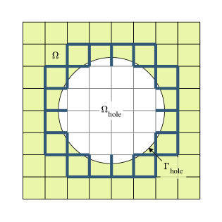
(a)

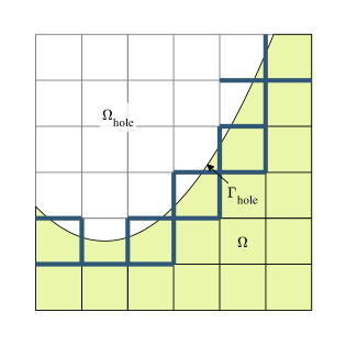
(b)

Figure 9: Illustrating the set of edges $\mathcal{F}$ on which the ghost penalty stabilization term is computed. Edges in $\mathcal{F}$ are bold. The element tessellation, $\mathcal{T}$, is an $8\times 8$ and a $6\times 6$ mesh of square elements in (a) and (b), respectively.

While the ghost penalty term improves matrix-conditioning, which enables more accurate calculation of eigenpairs using iterative or direct methods, it also introduces modes of deformation that can pollute the resulting band structure diagram. Frequencies of modes of deformation influenced by ghost penalty stabilization will appear in the band structure diagram if elastic wave speeds of the ghost penalty modes are less than the wave speeds of the non-ghost penalty modes of deformation. If ghost penalty modes appear in the band structure diagram, the ratio of $\beta_{K}$ to $\beta_{M}$ can be increased. An example of these modes polluting a band structure is demonstrated in Fig. 10(a). When $\beta_{M}$ is reduced by a factor of 4, the polluted modes no longer appear, as Fig. 10(b) reveals.

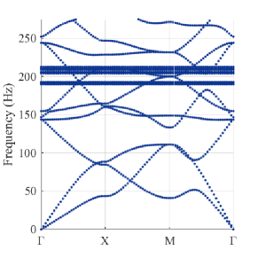
(a)

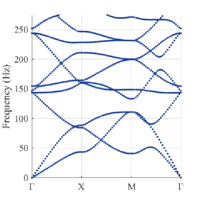
(b)

Figure 10: The effects of ghost penalty modes of deformation on the resulting band structure diagram. (a) Frequencies associated with the ghost penalty term appear in the band structure (horizontal lines) and (b) removing these modes by increasing the ratio $\beta_{K}/\beta_{M}$ by a factor of 4.

7 Numerical results

In this section, several examples are presented that demonstrate the capabilities of the X-FEM in modeling phononic crystals with voids and material interfaces and in generating band structure diagrams of these phononic crystals. We will focus on one-dimensional examples and two-dimensional examples that contain curved interfaces. Extended finite element solutions are generated from a code developed and run in MATLAB 9.9.0. The function eigs() is utilized to compute frequencies that satisfy the dispersion relationship for each periodic domain. Two-dimensional reference finite element solutions are generated using the multiphysics package COMSOL. In all extended finite element examples with voids, ghost penalty parameters of $\beta_{K}=1.0\times 10^{-8}$ and $\beta_{M}=2.5\times 10^{-9}$ are used.

7.1 Phononic crystal with circular void and square domain

In this example, we develop band structure diagrams for a phononic crystal with a circular void. This example has appeared in Wang et al. [83], and is repeated here using both the X-FEM and FEM. Using the X-FEM, the circle is exactly captured using a quadratic rational Bézier curve, whereas the FEM only approximates the shape of the circle. The square Bloch-periodic unit cell for this problem is illustrated in Fig. 11. The material properties are $E=20\ $\mathrm{GPa}\text{/}$$, $\nu=0.25$, and $\rho=2700\ $\mathrm{kg}\text{/}{\mathrm{m}}^{3}$$. The band structure diagram constructed using the X-FEM and FEM is presented in Fig. 12. The reference FEM band structure is generated from a finite element mesh with 227,824 DOFs (56,102 quadratic triangular finite elements) while the extended finite element band structure is generated from 16 quartic square finite elements (480 DOFs). The two solutions are observed to be nearly identical.

To quantitatively study the accuracy of the extended finite element approach, the error in frequency as a function of the number of DOFs is plotted in Fig. 13. Plots are provided for the error in the lowest frequency and the tenth-lowest frequency at both the X-point and the M-point. At the X-point, the reference solution for the lowest frequency is $21.7343273\ $\mathrm{Hz}\text{/}$$ and for the tenth-lowest frequency it is $264.87440\ $\mathrm{Hz}\text{/}$$. The reference solutions for the M-point are $14.2430873\ $\mathrm{Hz}\text{/}$$ for the lowest frequency and $226.458845\ $\mathrm{Hz}\text{/}$$ for the tenth-lowest frequency. Reference solutions are generated from a highly refined FEM mesh of quadratic triangles, containing 6,285,432 DOFs. The frequency from the extended finite element solution approaches the reference solution at a rate of $2p$, matching a priori error estimates for the FEM. For quadratic finite elements, a convergence rate of $4$ is observed in Fig. 13, which also matches the theoretical estimate. With the spectral X-FEM, accuracy per degree-of-freedom consistently increases with larger $p$, demonstrating the solution efficiency gains possible through spectral finite elements. To illustrate this point, with quartic extended finite elements, only about 4,000 DOFs are required to obtain accuracy on par with approximately 200,000 DOFs using a quadratic finite element mesh.

Solutions generated from the X-FEM require identification of elements cut by the void boundary, generating the parametric representation over the element of the boundary, and integrating element stiffness and mass matrices over the cut element using the HNI method. To quantify the impact of these tasks on the analysis run time, we measure the wall clock time required to perform each of them on each analysis run. To ensure consistent timing measurements, each task is repeated 100 times, and the average wall clock time is reported here. All timing results are generated on a Linux computer with an Intel Xeon E5-2695 v4 and 128 GB RAM running MATLAB 9.9.0. Time to identify cut elements and generate parametric representations of the boundary in each cut element versus the number of DOFs is reported in Fig. 14(a). From Fig. 14(a), we observe that the number of DOFs is linearly correlated to the wall clock time to complete these tasks. Since fewer elements per DOF are present as $p$ increases, fewer parametric representations of the circle need to be generated as $p$ grows. As a result, the wall clock time per DOF reduces as $p$ increases. The time to integrate the element stiffness and mass matrices ($\bm{K}_{e}$ and $\bm{M}_{e}$, respectively) in enriched and standard elements versus $p$ is displayed in Fig. 14(b). Overall, integrating element system matrices using HNI on cut elements increases the wall clock time by approximately a factor of 10. While the increase in time to integrate the element system matrices using HNI is considerable, we note integration remains a small portion of total wall clock time to compute the band structure. Furthermore, the additional time required to compute void boundary parametrizations and to integrate using the HNI method is in lieu of generating a conforming mesh—a nontrivial task that is required for the finite element solution. Finally, the performance of the MATLAB routines could likely be improved through further code optimizations, which were not investigated.

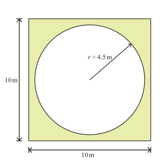
Figure 11: Unit cell geometry of a phononic crystal with a circular void.

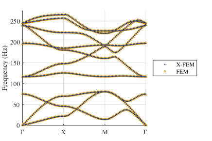
Figure 12: Band structure diagram for a phononic crystal with a circular void. Solution using quartic X-FEM (414 DOFs) and reference solution using quadratic FEM (227,824 DOFs).

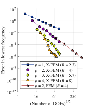
(a)

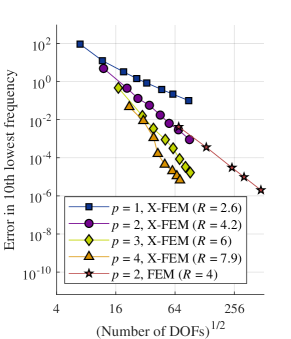
(b)

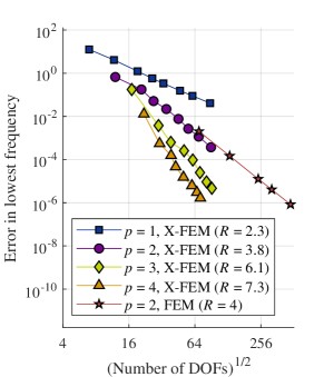
(c)

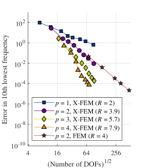
(d)

Figure 13: Error in frequency versus number of DOFs for the circular void example. (a) Lowest frequency at the X-point, (b) tenth lowest frequency at the X-point, (c) lowest frequency at the M-point, and (d) tenth lowest frequency at the M-point.

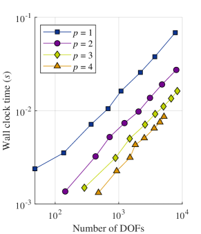
(a)

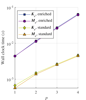
(b)

Figure 14: Wall clock time for X-FEM related routines in the circular void problem. (a) Wall clock time required to determine elements cut by the circular void and develop a parametric representation of the circle on each cut element versus number of DOFs and (b) wall clock time to integrate element system matrices versus $p$ for enriched and standard elements.

7.2 Phononic crystal with circular void and skew domain

In this example, the band structure of a skew unit cell with a circular void is generated. The geometry of the unit cell is illustrated in Fig. 15(a) and the material properties are repeated from Section 7.1; that is, $E=20\ $\mathrm{GPa}\text{/}$$, $\nu=0.25$, and $\rho=2700\ $\mathrm{kg}\text{/}{\mathrm{m}}^{3}$$. This choice of lattice vectors results in a regular hexagonal first Brillouin zone, which is illustrated in Fig. 15(b).

The band structure diagram is computed using both the FEM and the X-FEM. For the X-FEM, the problem is run with a $4\times 4$ element mesh of structured quartic elements, resulting in a total of 476 DOFs. The mesh is shown in Fig. 15(c). As is done in the example in Section 7.1, the circular void is modeled exactly using a quadratic rational Bézier curve. For the FEM, a mesh of quadratic triangular elements is utilized with a total of 7,632 DOFs (see Fig. 15(d)). With the FEM, the circular void is only approximated using quadratic polynomial curves. Band structure for the finite element and extended finite element solutions is presented in Fig. 15(e). Quantitatively, relative errors between the band structures range from $4.7\times 10^{-5}$ to $2.7\times 10^{-3}$.

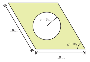
(a)

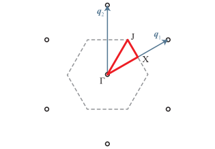
(b)

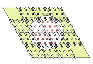
(c)

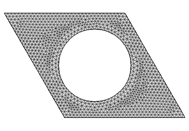
(d)

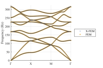
(e)

Figure 15: Skewed unit cell geometry of a phononic crystal with a circular void. (a) Problem setup, (b) first Brillouin zone on the reciprocal lattice (dashed line) and irreducible Brillouin zone (bold, red line), (c) extended finite element mesh (476 total DOFs; nodes with active DOFs are open circles and nodes with removed DOFs are red crosses), (d) finite element mesh (7,632 DOFs), and (e) band structure diagram.

7.3 Phononic crystal with elliptical void

Next, a band structure diagram is constructed for a phononic crystal whose Bloch-periodic domain contains an elliptical void. The material properties from Section 7.1 are repeated in this example and the unit cell geometry is illustrated in Fig. 16(a). The parameter $\theta$ is varied from $0$ to $\pi/4$ and the resulting size of the largest band gap in the first ten frequencies is plotted in Fig. 16(b). Two representative band structure diagrams are presented in Fig. 16(c) and Fig. 16(d), which are for $\theta=0$ and $\theta=\pi/4$, respectively. When $\theta=0$, a single band gap is present between approximately $100\ $\mathrm{Hz}\text{/}$$ and $125\ $\mathrm{Hz}\text{/}$$. When $\theta$ is increased to $\pi/4$, two band gaps are present at approximately $100\ $\mathrm{Hz}\text{/}$$ and $175\ $\mathrm{Hz}\text{/}$$. All extended finite element analyses of this problem are performed with a $4\times 4$ element mesh of quartic finite elements. The ellipse geometry is modeled exactly using rational quadratic Bézier curves to represent the void boundary.

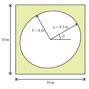
(a)

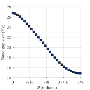
(b)

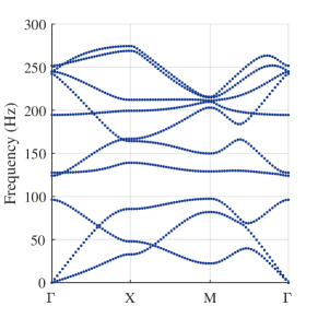
(c)

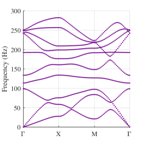
(d)

Figure 16: Unit cell geometry of a phononic crystal with an elliptical void. (a) Problem setup, (b) largest band gap versus angle $\theta$, (c) extended finite element band structure diagram for $\theta=0$, and (d) extended finite element band structure diagram for $\theta=\pi/4$.

7.4 Phononic crystal with a clover-shaped void

As the final void example, we consider a unit cell $\Omega=[-5,5]^{2}$ with a void defined by a level set function, which demonstrates the capability to model more general voids whose geometry may not be known explicitly. We choose the level set function

$$\varphi(r,\theta)=\frac{1}{5}r+\frac{2}{5}\sin^{4}\left(\frac{3}{2}\theta\right)-\frac{4}{5},$$ (51)

where $r=\sqrt{x^{2}+y^{2}}$ and $\theta=\tan^{-1}\left(\frac{y}{x}\right)$ are polar coordinates. The level set boundary is approximated using cubic Hermite functions, as described in Section 5.1. Rather than approximating the level set function using the finite element interpolant, we choose to use (51) directly in (38) and (39). This results in the cubic Hermite functions approximating the level set function directly, eliminating a source of error in the geometric description of the unit cell. The domain is modeled with 16 quartic extended finite elements arranged in a $4\times 4$ mesh. Material properties match those in Section 7.1. The meshed geometry is illustrated in Fig. 17(a) and the resulting band structure for the ten lowest frequencies is displayed in Fig. 17(c). The resulting band structure is in close agreement with one generated from a finite element analysis using quadratic triangular elements (mesh drawn in Fig. 17(b)). A maximum difference of $0.6\ $\mathrm{Hz}\text{/}$$ is observed between the finite element and extended finite element band structure diagrams.

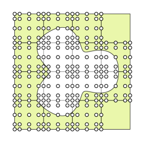
(a)

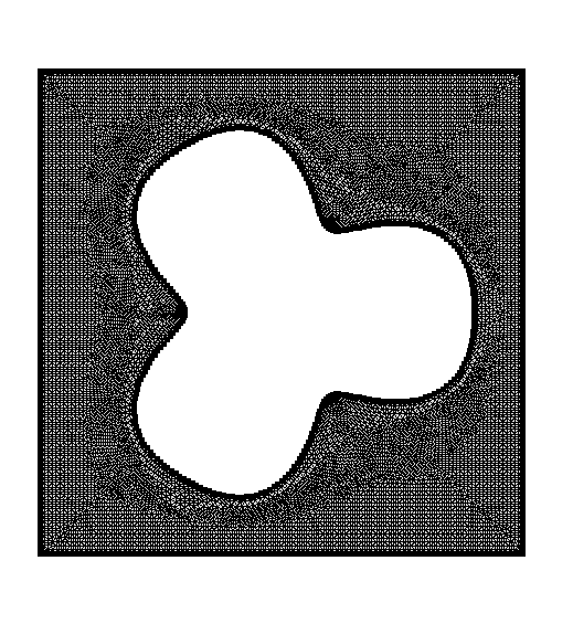
(b)

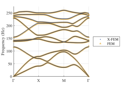
(c)

Figure 17: Unit cell geometry of a phononic crystal with a clover-shaped void. (a) extended finite element mesh (512 total DOFs; nodes with enriched DOFs are open circles), (b) finite element mesh (74,204 DOFs), and (c) band structure diagram.

7.5 One-dimensional two-phase phononic crystal

First, the application of the enrichment function for modeling material discontinuities in the X-FEM is presented in a one-dimensional setting. In one dimension, Rytov [84] derived an exact dispersive solution:

$$\cos(ka)=\cos\frac{\omega h_{1}}{c_{1}}\cos\frac{\omega h_{2}}{c_{2}}-\Gamma\sin\frac{\omega h_{1}}{c_{1}}\sin\frac{\omega h_{2}}{c_{2}},$$ (52a)

where

$$\Gamma=\frac{1+\kappa^{2}}{2\kappa},\qquad\kappa=\frac{\rho_{1}c_{1}}{\rho_{2}c_{2}},\qquad c_{i}=\sqrt{\frac{E_{i}}{\rho_{i}}}\quad(i=1,2).$$ (52b)

Following Lu and Srivastava [45], we choose the material properties $E_{1}=8\ $\mathrm{GPa}\text{/}$$, $\rho_{1}=1000\ $\mathrm{kg}\text{/}{\mathrm{m}}^{3}$$, $h_{1}=0.003\ $\mathrm{m}\text{/}$$, $E_{2}=300\ $\mathrm{GPa}\text{/}$$, $\rho_{2}=8000\ $\mathrm{kg}\text{/}{\mathrm{m}}^{3}$$, and $h_{2}=0.0013\ $\mathrm{m}\text{/}$$. The unit cell length is $a=h_{1}+h_{2}=0.0043\ $\mathrm{m}\text{/}$$. Given a frequency $f=\omega/(2\pi)$, (52) can be used to find a wavevector in the irreducible Brillouin zone, $Q:=ka/(2\pi)$ for $-0.5\leq Q\leq 0.5$ (or $0\leq Q\leq 0.5$ due to symmetry).

The problem is modeled using the FEM, the X-FEM, and the plane wave expansion method. For analyses conducted with finite elements, a three element mesh is used where two elements lie in the domain of material 1 and the domain of material 2 is modeled with one element. For extended finite element analyses, the mesh consists of two elements, and the inter-element node does not coincide with the location of the interface. Instead, (24) is used to capture the effect of the material interface in the interior of the element. The accuracy of the X-FEM and the FEM for these meshes is expected to be nearly identical provided $p$ is the same, since both are capable of representing the same piecewise continuous polynomial functions [55].

To examine the effect of $p$-refinement on solution accuracy, the problem is run with finite elements and extended finite elements of order $3$ to $12$. The band structure diagram for the case $p=5$ is presented in Fig. 18(b) and Fig. 18(a). This results in 16 DOFs for the finite element analysis and 17 DOFs for the extended finite element analysis. For the five lowest frequencies, the numerical solutions are indistinguishable from the exact band structure diagram using either the FEM or the X-FEM. Relative frequency error in the fifth-lowest frequency versus the number of degrees of freedom is plotted in Fig. 18(c) and Fig. 18(d) for $Q=0$ and $Q=0.5$, respectively. Convergence of both the finite element solution and the extended finite element solution is exponential with $p$-refinement.

(a)

(b)

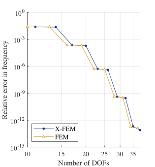
(c)

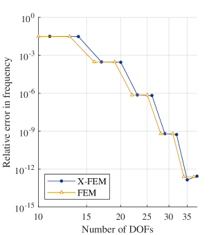
(d)

Figure 18: One-dimensional two-phase phononic crystal. (a) Band structure diagram using two fifth-order extended finite elements, (b) band structure diagram using three fifth-order finite elements, (c) convergence of the fifth-lowest frequency with $p$-refinement at $Q=0$, and (d) convergence of the fifth-lowest frequency with $p$-refinement at $Q=0.5$.

Finally, we examine the accuracy of the frequency solutions as a function of the ratio of $E_{1}$ to $E_{2}$. A total of 100 values of $E_{1}/E_{2}$ in between $E_{1}/E_{2}=1.0\times 10^{-3}$ to $E_{1}/E_{2}=1.0\times 10^{3}$ are tested in the numerical study, and the error in the lowest five frequencies as $E_{1}/E_{2}$ is varied is plotted at the point $Q=0.25$ in Fig. 19. The study is conducted with fifth-order spectral finite elements (16 DOFs), fifth-order extended spectral finite elements (17 DOFs), and using the plane wave expansion method (201 DOFs). Figure 19 demonstrates superior accuracy of spectral (extended) finite elements as compared to the plane wave expansion technique in two-phase materials. With a greater than $10$-fold reduction of DOFs, the FEM and the X-FEM deliver much better accuracy than the plane wave expansion method for the three lowest frequencies, and similar accuracy for the fourth and fifth frequency. The extended finite element solution contains slightly less error when compared to the finite element solution due to the extra degree of freedom in the extended finite element mesh, which allows $(p\!+\!1)$-th order terms to be partially captured (see Chin and Sukumar [55] for details).

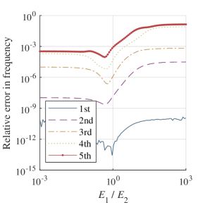
(a)

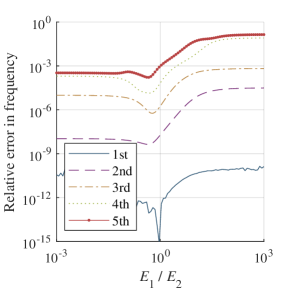
(b)

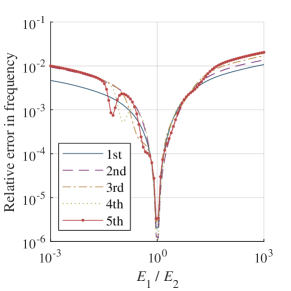
(c)

Figure 19: Error in relative frequency for the first through fifth lowest frequency for various ratios of $E_{1}$ to $E_{2}$. (a) Fifth-order extended finite elements (17 DOFs), (b) fifth-order spectral finite elements (16 DOFs), (c) plane wave expansion (201 DOFs).

7.6 Two-phase phononic crystal with circular inclusion

To study the performance of the enrichment function in a two-dimensional Bloch-periodic domain, we model a two-phase phononic crystal with a circular inclusion. The model problem, which appears in Srivastava and Nemat-Nasser [43], is illustrated in Fig. 20. Inside the circular inclusion, the material properties are $E_{2}=200\ $\mathrm{GPa}\text{/}$$, $\nu_{2}=0.3$ and $\rho_{2}=3300\ $\mathrm{kg}\text{/}{\mathrm{m}}^{3}$$. Over the remainder of the domain, the material properties are $E_{1}=2\ $\mathrm{GPa}\text{/}$$, $\nu_{1}=0.3$, and $\rho_{1}=1100\ $\mathrm{kg}\text{/}{\mathrm{m}}^{3}$$. The problem is analyzed using quadratic, triangular finite elements and the spectral X-FEM. Since enrichment using (24) requires a finite element interpolation of level set geometry, the parametric form of the interface location is approximated using cubic Hermite functions (see Section 5.1 for details). Reference solutions are generated using a finite element solution from a highly refined mesh (1,772,522 DOFs).

A band structure diagram for this problem using both finite elements and spectral extended finite elements is presented in Fig. 21. The extended finite element solution using a $4\times 4$ mesh of quartic finite elements (674 DOFs) is indistinguishable from the reference finite element solution. The convergence properties of both the spectral extended finite element and finite element solutions are examined through $h$-refinement studies in Fig. 22. Spectral extended finite elements of order $p=1,\dotsc,4$ and quadratic finite elements are utilized in the study. The error in the lowest and tenth-lowest frequency at the X-point and the M-point are considered. Reference solutions (computed on the reference finite element mesh) are $1.7029188\times 10^{5}\ $\mathrm{Hz}\text{/}$$ and $7.4091162\times 10^{5}\ $\mathrm{Hz}\text{/}$$ for the lowest and tenth lowest frequencies, respectively, at the X-point. At the M-point, the reference solution for the lowest frequency is $2.5329233\times 10^{5}\ $\mathrm{Hz}\text{/}$$ and for the tenth lowest frequency is $7.3191350\times 10^{5}\ $\mathrm{Hz}\text{/}$$. In the extended finite element analyses, the error in frequency reduces with an increase in the number of degrees of freedom at a rate of approximately $2p$ with all four values of $p$ tested, matching the a priori estimate for finite elements. With quadratic finite elements, error reduces at a rate of approximately $4$. As with the circular void problem, the quartic spectral extended finite element solution provides equivalent accuracy with substantially fewer degrees of freedom as compared to the quadratic finite element solution. For eight digits of accuracy in the frequency solution, approximately thirty-fold fewer DOFs are required when using the X-FEM.

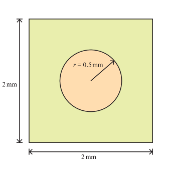
Figure 20: Unit cell geometry of a phononic crystal with a circular inclusion.

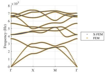
Figure 21: Band structure diagram for a phononic crystal with a circular inclusion. Solution using quartic extended finite elements (674 DOFs) and reference solution using quadratic finite elements (450,370 DOFs).

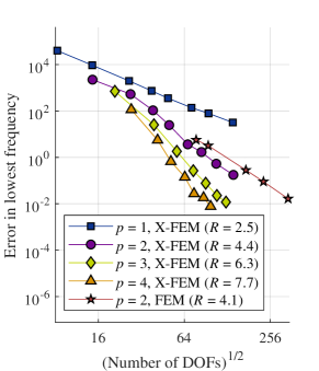
(a)

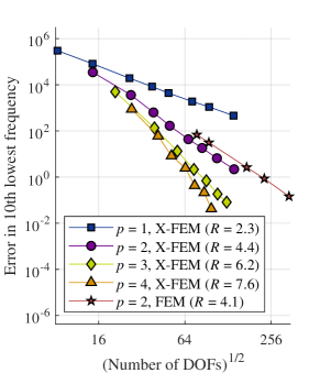
(b)

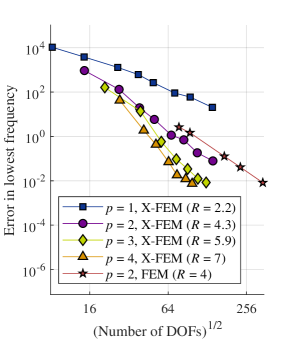
(c)

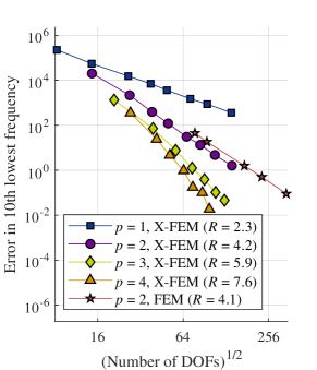
(d)

Figure 22: Error in frequency versus number of DOFs for the circular inclusion example. (a) Lowest frequency at the X-point, (b) tenth lowest frequency at the X-point, (c) lowest frequency at the M-point, and (d) tenth lowest frequency at the M-point.

7.7 Two-phase phononic crystal with ring inclusion

As a final example, we generate a band structure diagram for a two-phase phononic crystal with a ring-shaped inclusion. The unit cell geometry is illustrated in Fig. 23. In $\Omega_{I}$, the material properties are $E_{1}=2\ $\mathrm{GPa}\text{/}$$, $\nu_{1}=0.3$, and $\rho_{1}=1100\ $\mathrm{kg}\text{/}{\mathrm{m}}^{3}$$ and in $\Omega_{II}$, the material properties are $E_{2}=200\ $\mathrm{GPa}\text{/}$$, $\nu_{2}=0.3$, and $\rho_{2}=3300\ $\mathrm{kg}\text{/}{\mathrm{m}}^{3}$$. The band structure diagram is generated using both extended finite elements and finite elements. The meshes used to generate these solutions are illustrated in Fig. 24(a) and Fig. 24(b). With the extended finite element mesh, 16 quartic elements with 1,090 total DOFs are used. The level set zero is approximated using cubic Hermite functions, as described in Section 5.1. In comparison, the finite element mesh uses 7,600 quadratic triangular elements with 30,802 total DOFs. The band structure diagrams generated using the X-FEM and the FEM are displayed in Fig. 24(c). The diagrams match to approximately three significant digits. Also of note, a large band gap is present between the third and fourth frequency with this unit cell configuration and the fourth through tenth lowest frequencies are nearly constant as the wave vector varies, leading to additional band gaps.

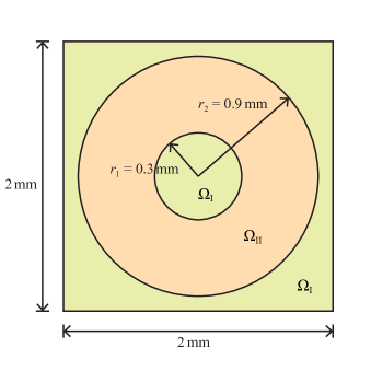
Figure 23: Unit cell geometry of a two-phase phononic crystal with a ring inclusion.

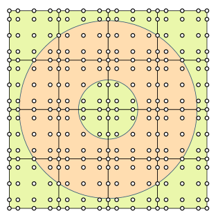
(a)

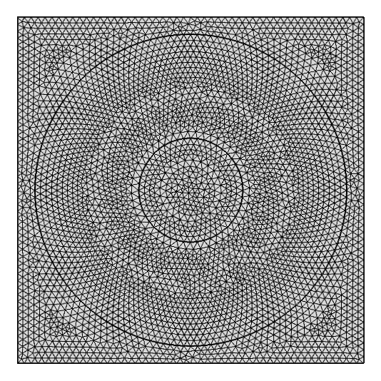
(b)

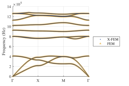
(c)

Figure 24: Band structure diagram for a phononic crystal with a ring inclusion. (a) Quartic extended finite element mesh (1,090 total DOFs; all nodes contain bimaterial enrichment), (b) quadratic finite element mesh (30,802 DOFs), and (c) band structure diagram.

8 Conclusions

In this paper, we introduced the spectral extended finite element method (X-FEM) for constructing band structure diagrams in phononic crystals. Using the X-FEM to represent boundaries with spectral finite elements requires accurate and robust interface reproduction on curved interfaces, accurate and efficient quadrature over curved interfaces, and an enrichment function over material interfaces that is capable of reproducing $p$-th order polynomials on both sides of the interface. Interface reproduction was accomplished using Bézier curves and approximating level set isocontours with cubic Hermite functions. Numerical quadrature was conducted using the homogeneous numerical integration (HNI) method, which represents boundary locations defined by parametric curves exactly, does not require partitioning elements cut by the interface, reduces integration to one dimensional integrals without any approximation, and gives accurate integration that is in fact exact when boundaries are affine or polynomial curves. Interfaces are captured through an enrichment function that is able to reproduce theoretical rates of convergence over curved interfaces [55] by accurately capturing the interface location and by providing linear, ridge-like enrichment on higher order elements. When combined, these methods demonstrated accurate band structure diagram reproduction on two-dimensional domains using minimal degrees of freedom.

The solution efficiency gains possible through spectral extended finite elements were demonstrated through several examples in Section 7. Band structure diagrams of phononic crystals with circular voids and circular inclusions converged much faster with a higher degree of polynomial reproduction. For example in the circular void problem, to reduce error in frequency to below $\mathcal{O}(10^{-5})$, 40–50 times more degrees of freedom were needed with quadratic finite elements as compared to quartic spectral extended finite elements. Typically, the utilization of spectral finite elements is limited by issues of mesh generation and open questions of polynomial reproduction with non-affine transformations of spectral elements. However, the framework of the spectral extended finite element method introduced in this paper eliminates these issues. Meshes are no longer required to conform to the locations of voids and material inclusions in phononic crystals; therefore, elements can remain aligned with the (affine) unit cell structure ensuring that the higher-order polynomial space is retained.

Eliminating the need for mesh generation and providing efficient generation of phononic band structure diagrams enables a more rapid understanding of the properties of various phononic crystals, and speeds up iterative design processes, including parametric studies and the design of improved phononic crystals using shape optimization and topology optimization. For the design and optimization of phononic crystals, level set representations of geometry are appealing since they allow for arbitrary smooth, curved boundaries. Level set methods have already been successfully applied to topology optimization and shape optimization [85, 86, 87], demonstrating the appeal of combining these ideas. For these applications, the use of the spectral X-FEM presented in this paper would be worth pursuing.

Declaration of competing interest

The authors declare that they have no known competing financial interests or personal relationships that could have appeared to influence the work reported in this paper.

Disclaimer

This document was prepared as an account of work sponsored by an agency of the United States government. Neither the United States government nor Lawrence Livermore National Security, LLC, nor any of their employees makes any warranty, expressed or implied, or assumes any legal liability or responsibility for the accuracy, completeness, or usefulness of any information, apparatus, product, or process disclosed, or represents that its use would not infringe privately owned rights. Reference herein to any specific commercial product, process, or service by trade name, trademark, manufacturer, or otherwise does not necessarily constitute or imply its endorsement, recommendation, or favoring by the United States government or Lawrence Livermore National Security, LLC. The views and opinions of authors expressed herein do not necessarily state or reflect those of the United States government or Lawrence Livermore National Security, LLC, and shall not be used for advertising or product endorsement purposes.

References

- [1] E. Yablonovitch, Inhibited spontaneous emission in solid-state physics and electronics, Phys. Rev. Lett. 58 (20) (1987) 2059.
- [2] S. John, Strong localization of photons in certain disordered dielectric superlattices, Phys. Rev. Lett. 58 (23) (1987) 2486–2489.
- [3] A. A. Mokhtari, Y. Lu, A. Srivastava, On the emergence of negative effective density and modulus in 2-phase phononic crystals, J. Mech. Phys. Solids 126 (2019) 256–271.
- [4] M.-H. Lu, L. Feng, Y.-F. Chen, Phononic crystals and acoustic metamaterials, Mater. Today 12 (2009) 34–42.
- [5] M. Maldovan, Sound and heat revolutions in phononics, Nat. 503 (7475) (2013) 209–217.
- [6] M. I. Hussein, M. J. Leamy, M. Ruzzene, Dynamics of phononic materials and structures: Historical origins, recent progress, and future outlook, Appl. Mech. Rev. 66 (4) (2014) 40802.
- [7] Z. Liu, X. Zhang, Y. Mao, Y. Y. Zhu, Z. Yang, C. T. Chan, P. Sheng, Locally resonant sonic materials, Science 289 (5485) (2000) 1734.
- [8] X. Yu, J. Zhou, H. Liang, Z. Jiang, L. Wu, Mechanical metamaterials associated with stiffness, rigidity and compressibility: A brief review, Prog. Mater. Sci. 94 (2018) 114–173.
- [9] F. Cervera, L. Sanchis, J. V. Sanchez-Perez, R. Martinez-Sala, C. Rubio, F. Meseguer, C. Lopez, D. Caballero, J. Sánchez-Dehesa, Refractive acoustic devices for airborne sound, Phys. Rev. Lett. 88 (2) (2001) 23902.
- [10] A. Khelif, A. Choujaa, B. Djafari-Rouhani, M. Wilm, S. Ballandras, V. Laude, Trapping and guiding of acoustic waves by defect modes in a full-band-gap ultrasonic crystal, Phys. Rev. B 68 (21) (2003) 214301.
- [11] R. Al Jahdali, Y. Wu, High transmission acoustic focusing by impedance-matched acoustic meta-surfaces, Appl. Phys. Lett. 108 (2016) 031902.
- [12] A. A. Mokhtari, Y. Lu, Q. Zhou, A. V. Amirkhizi, A. Srivastava, Scattering of in-plane elastic waves at metamaterial interfaces, International Journal of Engineering Science 150 (2020) 103278.
- [13] S. Yang, J. H. Page, Z. Liu, M. L. Cowan, C. T. Chan, P. Sheng, Focusing of sound in a 3D phononic crystal, Phys. Rev. Lett. 93 (2) (2004) 24301.
- [14] A. Sukhovich, L. Jing, J. H. Page, Negative refraction and focusing of ultrasound in two-dimensional phononic crystals, Phys. Rev. B 77 (1) (2008) 14301.
- [15] S. Zhang, L. Yin, N. Fang, Focusing ultrasound with an acoustic metamaterial network, Phys. Rev. Lett. 102 (2009) 194301.
- [16] S. C. S. Lin, T. J. Huang, J. H. Sun, T. T. Wu, Gradient-index phononic crystals, Phys. Rev. B 79 (9) (2009) 94302.
- [17] Y. Chen, H. Liu, M. Reilly, H. Bae, M. Yu, Enhanced acoustic sensing through wave compression and pressure amplification in anisotropic metamaterials, Nat. Commun. 5 (2018) 5247.
- [18] B. Liang, G. X. S., J. Tu, D. Zhang, J. C. Cheng, An acoustic rectifier, Nat. Mater. 9 (2010) 989–992.
- [19] J. Mei, G. Ma, M. Yang, Z. Yang, W. Wen, P. Sheng, Dark acoustic metamaterials as super absorbers for low-frequency sound, Nat. Commun. 3 (2012) 756.
- [20] R. Fleury, D. L. Sounas, C. F. Sieck, M. R. Haberman, A. Alù, Sound isolation and giant linear nonreciprocity in a compact acoustic circulator, Science 9 (2014) 989–992.
- [21] S. Yang, J. H. Page, Z. Liu, M. L. Cowan, C. T. Chan, P. Sheng, Ultrasound tunneling through 3D phononic crystals, Phys. Rev. Lett. 88 (10) (2002) 104301.
- [22] E. J. Reed, M. Soljačić, J. D. Joannopoulos, Reversed Doppler effect in photonic crystals, Phys. Rev. Lett. 91 (13) (2003) 133901.
- [23] S. L. Zhai, X. P. Zhao, S. Liu, F. L. Shen, L. L. Li, C. R. Luo, Inverse Doppler effects in broadband acoustic metamaterials, Sci. Rep. 6 (2016) 32388.
- [24] T. Gorishnyy, C. K. Ullal, M. Maldovan, G. Fytas, E. L. Thomas, Hypersonic phononic crystals, Phys. Rev. Lett. 94 (11) (2005) 115501.
- [25] R. Van Laer, B. Kuyken, D. Van Thourhout, R. Baets, Interaction between light and highly confined hypersound in a silicon photonic nanowire, Nat. Photonics 9 (2015) 199–203.
- [26] P. Arrangoiz-Arriola, E. A. Wollack, M. Pechal, J. D. Witmer, J. T. Hill, A. H. Safavi-Naeini, Coupling a superconducting quantum circuit to a phononic crystal defect cavity, Phys. Rev. X 8 (2018) 031007.
- [27] M. S. Kushwaha, P. Halevi, L. Dobrzynski, B. Djafari-Rouhani, Acoustic band structure of periodic elastic composites, Phys. Rev. Lett. 71 (13) (1993) 2022–2025.
- [28] O. Sigmund, J. S. Jensen, Systematic design of phononic band–gap materials and structures by topology optimization, Philos. Trans. A Math. Phys. Eng. Sci. 361 (1806) (2003) 1001–1019.
- [29] A. R. Diaz, A. G. Haddow, L. Ma, Design of band-gap grid structures, Struct. Multidiscipl. Optim. 29 (6) (2005) 418–431.
- [30] S. Halkjær, O. Sigmund, J. S. Jensen, Maximizing band gaps in plate structures, Struct. Multidiscipl. Optim. 32 (4) (2006) 263–275.
- [31] C. J. Rupp, A. Evgrafov, K. Maute, M. L. Dunn, Design of phononic materials/structures for surface wave devices using topology optimization, Struct. Multidiscipl. Optim. 34 (2) (2007) 111–121.
- [32] O. R. Bilal, M. I. Hussein, Ultrawide phononic band gap for combined in-plane and out-of-plane waves, Phys. Rev. E 84 (6) (2011) 65701.
- [33] S. Nemat-Nasser, J. R. Willis, A. Srivastava, A. V. Amirkhizi, Homogenization of periodic elastic composites and locally resonant sonic materials, Phys. Rev. B 83 (10) (2011) 104103.
- [34] A. A. Mokhtari, Y. Lu, A. Srivastava, On the properties of phononic eigenvalue problems, J. Mech. Phys. Solids 131 (2019) 167–179.
- [35] K. M. Ho, C. T. Chan, C. M. Soukoulis, Existence of a photonic gap in periodic dielectric structures, Phys. Rev. Lett. 65 (25) (1990) 3152.
- [36] M. M. Sigalas, E. N. Economou, Elastic and acoustic wave band structure, J. Sound Vib. 158 (1992) 377–382.
- [37] M. Sigalas, E. N. Economou, Band structure of elastic waves in two dimensional systems, Solid State Commun. 86 (3) (1993) 141–143.
- [38] M. S. Kushwaha, P. Halevi, G. Martinez, L. Dobrzynski, B. Djafari-Rouhani, Theory of acoustic band structure of periodic elastic composites, Phys. Rev. B 49 (4) (1994) 2313.
- [39] K.-J. Bathe, E. L. Wilson, Numerical methods in finite element analysis, Prentice-Hall, Englewood Cliffs, NJ, 1976.
- [40] S. Nemat-Nasser, Harmonic waves in layered composites, J. Appl. Mech. 39 (1972) 850.
- [41] S. Nemat-Nasser, F. C. L. Fu, S. Minagawa, Harmonic waves in one-, two-and three-dimensional composites: Bounds for eigenfrequencies, Int. J. Solids Struct. 11 (5) (1975) 617.
- [42] S. Minagawa, S. Nemat-Nasser, Harmonic waves in three-dimensional elastic composites, Int. J. Solids Struct. 12 (11) (1976) 769.
- [43] A. Srivastava, S. Nemat-Nasser, Mixed-variational formulation for phononic band-structure calculation of arbitrary unit cells, Mech. Mater. 74 (2014) 67–75.
- [44] I. Babuška, J. E. Osborn, Numerical treatment of eigenvalue problems for differential equations with discontinuous coefficients, Math. Comput. 32 (1978) 991.
- [45] Y. Lu, A. Srivastava, Variational methods for phononic calculations, Wave Motion 60 (2016) 46–61.
- [46] M. Kafesaki, E. N. Economou, Multiple-scattering theory for three-dimensional periodic acoustic composites, Phys. Rev. B 60 (17) (1999) 11993.
- [47] Z. Liu, C. T. Chan, P. Sheng, A. L. Goertzen, J. H. Page, Elastic wave scattering by periodic structures of spherical objects: Theory and experiment, Phys. Rev. B 62 (4) (2000) 2446.
- [48] M. Sigalas, M. S. Kushwaha, E. N. Economou, M. Kafesaki, I. E. Psarobas, W. Steurer, Classical vibrational modes in phononic lattices: theory and experiment, Z. Kristallogr. Cryst. Mater. 220 (9-10) (2005) 765–809.
- [49] R. L. Chern, C. C. Chang, C. C. Chang, R. R. Hwang, Large full band gaps for photonic crystals in two dimensions computed by an inverse method with multigrid acceleration, Phys. Rev. E 68 (2) (2003) 26704.
- [50] F. Casadei, J. J. Rimoli, M. Ruzzene, Multiscale finite element analysis of elastic wave scattering from localized defects, Finite Elem. Anal. Des. 88 (2014) 1–15.
- [51] M. I. Hussein, Reduced Bloch mode expansion for periodic media band structure calculations, Proc. R. Soc. Lond. A Math. Phys. Sci. 465 (2109) (2009) 2825.
- [52] D. Krattiger, M. I. Hussein, Bloch mode synthesis: Ultrafast methodology for elastic band-structure calculations, Phys. Rev. E 90 (6) (2014) 63306.
- [53] A. Srivastava, GPU accelerated variational methods for fast phononic eigenvalue solutions, in: SPIE Smart Structures and Materials+ Nondestructive Evaluation and Health Monitoring, International Society for Optics and Photonics, 2015, pp. 94381F–94381F.
- [54] A. Legay, H. W. Wang, T. Belytschko, Strong and weak arbitrary discontinuities in spectral finite elements, Int. J. Numer. Methods Eng. 64 (2005) 991–1008.
- [55] E. B. Chin, N. Sukumar, Modeling curved interfaces without element-partitioning in the extended finite element method, Int. J. Numer. Methods Eng. 120 (5) (2019) 607–649.
- [56] I. A. Veres, T. Berer, Complexity of band structures: Semi-analytical finite element analysis of one-dimensional surface phononic crystals, Phys. Rev. B 86 (10) (2012) 104304.
- [57] A.-C. Hladky-Hennion, J.-N. Decarpigny, Analysis of the scattering of a plane acoustic wave by a doubly periodic structure using the finite element method: Application to Alberich anechoic coatings, J. Acoust. Soc. Am. 90 (6) (1991) 3356–3367.
- [58] G. E. Karniadakis, S. J. Sherwin, Spectral/hp Element Methods for CFD, Oxford University Press, Oxford, UK, 1999.
- [59] Z.-J. Wu, F.-M. Li, Y.-Z. Wang, Study on vibration characteristics in periodic plate structures using the spectral element method, Acta Mech. 224 (2013) 1089–1101.
- [60] L. Shi, N. Liu, J. Zhou, Y. Zhou, J. Wang, Q. H. Liu, Spectral element method for band-structure calculations of 3D phononic crystals, J. Phys. D: Appl. Phys. 49 (2016) 455102.
- [61] Y. Cao, Z. Hou, Y. Liu, Convergence problem of plane-wave expansion method for phononic crystals, Phys. Lett. A 327 (2) (2004) 247–253.
- [62] I. Fried, Accuracy and condition of curved (isoparametric) finite elements, J. Sound Vib. 31 (3) (1973) 345–355.
- [63] O. C. Zienkiewicz, R. L. Taylor, The Finite Element Method, Volume 1: The Basis, 5th Edition, Butterworth Heinemann, Oxford, U.K., 2000.
- [64] R. Sevilla, S. Fernández-Méndez, A. Huerta, Comparison of high-order curved finite elements, Int. J. Numer. Methods Eng. 87 (2011) 719–734.
- [65] N. Moës, J. Dolbow, T. Belytschko, A finite element method for crack growth without remeshing, Int. J. Numer. Methods Eng. 46 (1999) 131–150.
- [66] J. Zhao, Y. Li, W. K. Liu, Predicting band structure of 3D mechanical metamaterials with complex geometry via XFEM, Comput. Mech. 55 (2015) 659–672.
- [67] N. Sukumar, J. E. Pask, Classical and enriched finite element formulation for Bloch-periodic boundary conditions, Int. J. Numer. Methods Eng. 77 (2009) 1121–1138.
- [68] E. Burman, Ghost penalty, C. R. Math. 348 (21–22) (2010) 1217–1220.
- [69] J. M. Melenk, I. Babuška, The partition of unity finite element method: Basic theory and applications, Comput. Methods Appl. Mech. Eng. 139 (1996) 289–314.
- [70] I. Babus̆ka, J. M. Melenk, The partition of unity method, Int. J. Numer. Methods Eng. 40 (4) (1997) 727–758.
- [71] I. Babus̆ka, U. Banerjee, K. Kergrene, Strongly stable generalized finite element method: Application to interface problems, Comput. Methods Appl. Mech. Eng. 327 (2017) 58–92.
- [72] C. Daux, N. Moës, J. Dolbow, N. Sukumar, T. Belytschko, Arbitrary branched and intersecting cracks with the extended finite element method, Int. J. Numer. Methods Eng. 48 (12) (2000) 1741–1760.
- [73] N. Sukumar, D. L. Chopp, N. Moës, T. Belytschko, Modeling holes and inclusions by level sets in the extended finite-element method, Comput. Methods Appl. Mech. Eng. 190 (2001) 6183–6200.
- [74] J. Chessa, H. Wang, T. Belytschko, On the construction of blending elements for local partition of unity enriched finite elements, Int. J. Numer. Methods Eng. 57 (2003) 1015–1038.
- [75] N. Moës, M. Cloirec, C. P., J.-F. Remacle, A computational approach to handle complex microstructure geometries, Comput. Methods Appl. Mech. Eng. 192 (2003) 3163–3177.
- [76] R. Alberdi, G. Zhang, K. Khandelwal, An isogeometric approach for analysis of phononic crystals and elastic metamaterials with complex geometries, Comput. Mech. 62 (2018) 285–307.
- [77] G. E. Farin, Curves and Surfaces for Computer-Aided Geometric Design: A Practical Guide, 4th Edition, Academic Press, New York, NY, 1996.
- [78] J. B. Lasserre, Integration on a convex polytope, Proc. Am. Math. Soc. 126 (8) (1998) 2433–2441.
- [79] E. B. Chin, J. B. Lasserre, N. Sukumar, Numerical integration of homogeneous functions on convex and nonconvex polygons and polyhedra, Comput. Mech. 56 (6) (2015) 967–981.
- [80] F. de Prenter, C. V. Verhoosel, G. J. van Zwieten, E. H. van Brummelen, Condition number analysis and preconditioning of the finite cell method, Comput. Methods Appl. Mech. Eng. 316 (2017) 297–327.
- [81] E. Burman, S. Claus, P. Hansbo, M. G. Larson, A. Massing, CutFEM: Discretizing geometry and partial differential equations, Int. J. Numer. Methods Eng. 104 (7) (2015) 472–501.
- [82] S. Sticko, G. Ludvigsson, G. Kreiss, High order cut finite elements for the elastic wave equation, Adv. Comput. Math. 46 (2020) 45.
- [83] Y.-F. Wang, Y.-S. Wang, X.-X. Su, Large bandgaps of two-dimensional phononic crystals with cross-like holes, J. Appl. Phys. 110 (2011) 113520.
- [84] S. M. Rytov, Acoustical properties of a thinly laminated medium, Sov. Phys.-Acoust. 2 (1956) 68.
- [85] S. Osher, F. Santosa, Level set methods for optimization problems involving geometry and constraints I. Frequencies of a two-density inhomogeneous drum, J. Comput. Phys. 171 (2001) 272–288.
- [86] M. Y. Wang, X. Wang, D. Guo, A level set method for structural topology optimization, Comput. Methods Appl. Mech. Eng. 192 (2003) 227–246.
- [87] G. Allaire, F. Jouve, A.-M. Toader, Structural optimization using sensitivity analysis and a level-set method, J. Comput. Phys. 194 (2004) 363–393.