Large $|k|$ behavior of complex geometric optics solutions to d-bar problems

Abstract.

Complex geometric optics solutions to a system of d-bar equations appearing in the context of electrical impedance tomography and the scattering theory of the integrable Davey-Stewartson II equations are studied for large values of the spectral parameter $k$. For potentials $q\in\langle\cdot\rangle^{-2}H^{s}(\mathbb{C})$ for some $s\in]1,2]$, it is shown that the solution converges as the geometric series in $1/|k|^{s-1}$. For potentials $q$ being the characteristic function of a strictly convex open set with smooth boundary, this still holds with $s=3/2$ i.e., with $1/\sqrt{|k|}$ instead of $1/|k|^{s-1}$. The leading order contributions are computed explicitly. Numerical simulations show the applicability of the asymptotic formulae for the example of the characteristic function of the disk.

1. Introduction

This paper is concerned with the large $|k|$ behavior of solutions to the Dirac system

(1.1) $$\begin{cases}\bar{\partial}\phi_{1}=\frac{1}{2}q\mathrm{e}^{\bar{k}\bar{z}-kz}\phi_{2},\\ \partial\phi_{2}=\sigma\frac{1}{2}\bar{q}\mathrm{e}^{kz-\bar{k}\bar{z}}\phi_{1},\quad\sigma=\pm 1,\end{cases}$$

subject to the asymptotic conditions

(1.2) $$\lim_{|z|\to\infty}\phi_{1}=1,\quad\lim_{|z|\to\infty}\phi_{2}=0;$$

here $q=q(x,y)$ is a complex-valued field, the spectral parameter $k\in\mathbb{C}$ is independent of $z=x+\mathrm{i}y$, and

$$\partial:=\frac{1}{2}\left(\frac{\partial}{\partial x}-\mathrm{i}\frac{\partial}{\partial y}\right)\quad\text{and}\quad\bar{\partial}:=\frac{1}{2}\left(\frac{\partial}{\partial x}+\mathrm{i}\frac{\partial}{\partial y}\right).$$

The functions $\phi_{i}(z;k)$, $i=1,2$ depend on $z$ and $k$ where it is understood that they need not be holomorphic in either variable.

As discussed in more detail in Subsection 1.1, the solutions to the system (1.1), subject to (1.2) are complex geometric optics (CGO) solutions to a d-bar problem. The latter appears in the scattering theory of two-dimensional integrable equations as the Davey-Stewartson (DS) equation (1.7), in electrical impedance tomography (EIT) and in the theory of random matrix models. Of special interest in the context of the DS equation is the reflection coefficient $R$, where

(1.3) $$\bar{R}=\frac{2\sigma}{\pi}\int_{\mathbb{C}}\mathrm{e}^{kz-\bar{k}\bar{z}}\bar{q}(z)\phi_{1}(z;k)d^{2}z,$$

which can be seen as a nonlinear analog to the Fourier transform of the potential $q$.

The existence and uniqueness of CGO solutions to system (1.1) with $\sigma=1$ was studied in [3] for Schwartz class potentials and in [25, 26, 27] for potentials $q\in L^{\infty}(\mathbb{C})\cap L^{1}(\mathbb{C})$ such that also $\hat{q}\in L^{\infty}(\mathbb{C})\cap L^{1}(\mathbb{C})$ where $\hat{q}$ is the Fourier transform of $q$ (the potentials have to satisfy a smallness condition in the focusing case). The results for system (1.1) for Schwartz class potentials were generalized respectively to real-valued, compactly supported potentials in $L^{p}(\mathbb{C})$ [6] and to potentials in $H^{1,1}(\mathbb{C})$ [24], and in [23] to potentials in $L^{2}(\mathbb{C})$.

For potentials $q$ in the Schwartz class of rapidly decreasing smooth potentials, the reflection coefficient (1.3) is also in the Schwartz class. However, the dependence of $\phi_{i}$, $i=1,2$ and $R$ on $k$ is much less clear for potentials $q$ of lower regularity, such as potentials with compact support, or slow decrease towards infinity, which are both important in EIT. It is the purpose of the present paper to give the large $|k|$ behaviour of the solutions to the system 1.1 for such cases.

The importance of d-bar problems in applications has led to many numerical approaches to solve them. The standard method is to use that the inverse of the d-bar operator is given by the solid Cauchy transform, a weakly singular integral which was first computed in the current context in [20], see [21] for a review of more recent developments, with Fourier methods and a simple regularization of the integrand. These approaches are of first order which means the numerical error decreases linearly with the number of Fourier modes. The first Fourier approach with an exponential decrease of the numerical error with the number of Fourier modes, or spectral convergence, was presented in [14, 15] for Schwartz class potentials via an analytical regularization of the integrand in the solid Cauchy transform. For potentials with compact support on a disk, a numerical approach of formally infinite order was presented in [19] based on a formulation of the problem in polar coordinates and the solution of the resulting system by a Chebyshev-Fourier method. As will be shown in this paper, the reflection coefficient (1.3) decreases algebraically in $1/|k|$ in this case as $|k|\to\infty$. Thus in contrast to the case of Schwartz potentials, a purely numerical approach cannot be of the order of machine precision (here $10^{-16}$) for all values of $k$. One of the motivations for the present paper is to present, in the concrete example of the characteristic function of the disk as the potential $q$, formulae for the large $|k|$ behaviour which together with the numerical approach [19] yield a complete description of the solutions in the whole complex $k$ plane within a predetermined accuracy. This gives an upper bound on the reflection coefficient, and we hope to be able to push the methods further for the leading asymptotics.

An interesting question in the context of the DS equation is the appearance of dispersive shock waves (DSWs), zones of rapid modulated oscillations in the vicinity of shocks in the semi-classical DS system for the same initial data. Such DSWs were studied numerically in [16]. A first attempt towards an asymptotic description of DSWs based on inverse scattering techniques was presented in [2]. Note that the first system for which a rather complete asymptotic description of DSWs exists is the completely integrable Korteweg-de Vries (KdV) equation. Historically the Gurevitch-Pitaevskii (GP) work [12] on solutions to the KdV equation for steplike initial data was very influential. It was one of the motivation of the numerical work [19] to provide numerical tools for the study of the corresponding GP problem for DS II, initial data given by the characteristic function of the disk. In the present work, this case is addressed in some detail.

1.1. Applications of the Dirac system

The system (1.1) and the conditions (1.2) are equivalent to the Dirac system (simply put $\phi_{1}:=\psi_{1}e^{-kz}$, $\phi_{2}:=\psi_{2}e^{-\overline{kz}}$)

(1.4) $$\begin{array}[]{l}\bar{\partial}\psi_{1}=\frac{1}{2}q\psi_{2},\\ {}\\ \partial\psi_{2}=\sigma\frac{1}{2}\bar{q}\psi_{1},\quad\sigma=\pm 1\end{array}$$

where the scalar functions $\psi_{1}$ and $\psi_{2}$ satisfy the CGO asymptotic conditions

(1.5) $$\begin{array}[]{l}\lim_{|z|\to\infty}\psi_{1}\mathrm{e}^{-kz}=1,\\ {}\\ \lim_{|z|\to\infty}\psi_{2}\mathrm{e}^{-\bar{k}\bar{z}}=0.\end{array}$$

Putting $\Psi_{\pm}:=\psi_{1}\pm\bar{\psi}_{2}$, the system (1.4) is diagonalized,

(1.6) $$\bar{\partial}\Psi_{\pm}=\pm\frac{1}{2}q\bar{\Psi}_{\pm}$$

subject to the asymptotic condition $\lim_{|z|\to\infty}\Psi_{\pm}\mathrm{e}^{-kz}=1$. The disadvantage of equation (1.6) is that it is not complex linear in $\Psi_{\pm}$, which is why we use the system (1.4).

The system (1.4) has many applications, the first being in completely integrable equations in two dimensions. As was shown in [9, 10] system (1.4) gives both the scattering and inverse scattering map for the Davey-Stewartson II equation

(1.7) $$\begin{split}iq_{t}+(q_{xx}-q_{yy})+2\sigma(\Phi+|q|^{2})q&=0,\\ \Phi_{xx}+\Phi_{yy}+2(|q|^{2})_{xx}&=0,\end{split}$$

a two-dimensional nonlinear Schrödinger equation; here the parameter $\sigma=1$ in the defocusing case, and $\sigma=-1$ in the focusing case. DS systems, which are in general not integrable, appear in the modulational regime of many dispersive equations as for instance the water wave systems, see e.g., [17] for a review on DS equations and a comprehensive list of references.

In the smooth case the scattering data are given in terms of the reflection coefficient $R=R(k)$ in terms of $\psi_{2}(z;k)$ as follows (in the general case, one has to consider (1.3)):

(1.8) $$\mathrm{e}^{-kz}\overline{\psi_{2}(z;k)}=\frac{1}{2}R(k)z^{-1}+O(|z|^{-2}),\quad|z|\to\infty,$$

which is equivalent to (1.3) after writing $\phi_{2}$ as the solid Cauchy transform of the right hand side of the second equation of (1.1) and taking the limit $z\to\infty$. Note that the understanding of the Dirac system (1.1) with $\sigma=-1$ is much less complete than in the defocusing case $\sigma=1$. In the former case the system no longer has generically a unique solution for large classes of potentials $q$ for all $k\in\mathbb{C}$. There can be special values of the spectral parameter, called exceptional points, where the system is not uniquely solvable. Therefore we concentrate for the examples (which cover all values of $k\in\mathbb{C}$) on the defocusing case. But the results for large $|k|$ we present in this paper hold for both cases. Note that this implies that the exceptional points can only occur in a bounded set. Perry [5] gave a bound for the radius of this set based on the $H^{1,1}$ norm of the potential. It is beyond the scope of the current paper to establish similar bounds based on our approach.

As $q$ in (1.7) evolves in time $t$, the reflection coefficient evolves by a trivial phase factor:

(1.9) $$R(k;t)=R(k,0)e^{4it\Re(k^{2})}.$$

The inverse scattering transform for DS II is then given by (1.4) and (1.5) after replacing $q$ by $R$ and vice versa, the derivatives with respect to $z$ by the corresponding derivatives with respect to $k$, and asymptotic conditions for $k\to\infty$ instead of $z\to\infty$, see [1].

Systems of the form (1.4) also appear in electrical impedance tomography (EIT) in 2d, the reconstruction of the conductivity in a given domain $\Omega$ from measurements of the electrical current through its boundary, induced by an applied voltage, i.e., from the Dirichlet-to-Neumann map. This problem was first posed by Calderón [7] and bears his name. For a comprehensive review of the mathematical aspects and advances see [28, 21]. The basic idea of EIT is to construct CGO solutions to the conductivity equation in some domain $\Omega\in\mathbb{R}^{2}$,

(1.10) $$\nabla\cdot(\sigma(x,y)\nabla u(x,y))=0,\quad(x,y)\in\Omega.$$

In [6], this was done in form of the system (1.4) by putting $q=-(1/2)\partial\ln\sigma$ for conductivities $\sigma\in C^{1}(\Omega)$. The CGO solutions satisfy slightly different asymptotic conditions in this case which is why we study larger classes of conditions than (1.5). The reconstruction of the conductivity from the Dirichlet-to-Neumann map is also achieved via a d-bar problem, see [28].

D-bar problems also appear in the context of 2d orthogonal polynomials, and of Normal Matrix Models in Random Matrix Theory, see e.g. [14].

1.2. Main results

1. The d-bar equation on $\mathbb{C}$

For $s\in\mathbb{R}$, we write $\langle\cdot\rangle^{s}L^{2}=\left\{\langle z\rangle^{s}u(z);u\in L^{2}(\mathbb{C})\right\}$, where $\langle z\rangle^{s}=(1+|z|^{2})^{1/2}$. Thus $||\tilde{u}||_{\langle z\rangle^{s}L^{2}}=||u||_{L^{2}}$ if $\tilde{u}=\langle z\rangle^{s}u\in\langle\cdot\rangle^{s}L^{2}(\mathbb{C})$.
Reviewing Hörmander’s approach with Carleman estimates, we show in the propositions 2.1, 2.2 that if $0<\epsilon\leq 1$, then for every $v\in\langle\cdot\rangle^{\epsilon-2}L^{2}(\mathbb{C})$ the equation $\overline{\partial}u=v$ in (2.10) has a unique solution $u\in\langle\cdot\rangle^{\epsilon}L^{2}$. When $\epsilon=1$ we show in Proposition 2.3 that when $v\in\langle\cdot\rangle^{-1}L^{2}$ the unique solution $u\in\langle\cdot\rangle L^{2}$ is given by the standard formula (2.16),

$$u(z)=\frac{1}{\pi}\int\frac{1}{z-w}v(w)L(dw),$$

where $L(dw)$ denotes the Lebesgue measure on $\mathbb{C}\simeq\mathbb{R}^{2}$. Of course we have the same results for the complex conjugate equation $\partial u=v$ and we then have to replace $1/(z-w)$ with $1/(\overline{z}-\overline{w})$ in the integral above.

We are interested in the case when $|k|$ is large and notice that

(1.11) $$kz-\overline{kz}=i|k|\Re(z\overline{\omega})=i|k|\langle z,\omega\rangle_{\mathbb{R}^{2}},\ \ \omega=\frac{2i\overline{k}}{|k|},$$

so that $|\omega|=2$. Here we identify $\mathbb{C}\simeq\mathbb{R}^{2}$ in the usual way. Introduce the semi-classical parameter $h=1/|k|$, $0<h\ll 1$ and put

$$\widehat{\tau}_{\omega}u(z)=e^{\frac{i}{h}\langle z,\omega\rangle_{\mathbb{R}^{2}}}u(z).$$

$\widehat{\tau}_{\omega}$ is translation by $\omega\in\mathbb{R}^{2}$ on the $h$-Fourier transform side, see (3.9).

For $v\in\langle\cdot\rangle^{-1}L^{2}$, let $u$, $\widetilde{u}$ be the unique solutions in $\langle\cdot\rangle L^{2}$ (see Section 2) of the equations

(1.12) $$h\overline{\partial}u=v,\ h\partial\widetilde{u}=v,$$

and write $u=Ev$, $\widetilde{u}=Fv$.

The goal is to solve the system (1.1) iteratively for small $h$. With the above notation this implies that we can write (1.1) in the form ($\phi_{i}\in\langle\cdot\rangle^{-1}L^{2}$, $i=1,2$)

(1.13) $$\begin{cases}\phi_{1}-E\widehat{\tau}_{-\omega}\frac{hq}{2}\phi_{2}=E\Psi_{1},\\ \phi_{2}-\sigma F\widehat{\tau}_{\omega}\frac{h\overline{q}}{2}\phi_{1}=F\Psi_{2},\end{cases}$$

with $\Psi_{1}=\Psi_{2}=0$, or

(1.14) $$(1-\mathcal{K})\begin{pmatrix}\phi_{1}\\ \phi_{2}\end{pmatrix}=\begin{pmatrix}E\Psi_{1}\\ F\Psi_{2}\end{pmatrix},$$

where

(1.15) $$\mathcal{K}=\begin{pmatrix}0&A\\ B&0\end{pmatrix},\ \ \begin{cases}A=E\widehat{\tau}_{-\omega}\frac{hq}{2},\\ B=\sigma F\widehat{\tau}_{\omega}\frac{h\overline{q}}{2}\ (=\sigma\overline{A})\end{cases}.$$

The inhomogeneities $\Psi_{1}$, $\Psi_{2}$ are introduced in the above system to allow for an iterative solution in $h$. In leading order they depend on the asymptotic conditions, e.g. (1.2), which will not be specified for the moment in order to allow for rather general conditions.

2. Inverting the system

Let $q\in\langle\cdot\rangle^{-2}H^{s}(\mathbb{C})$ for some $s\in]1,2]$ and fix $\epsilon\in]0,1]$. Then $\mathcal{K}^{2}=\mathcal{O}(h^{s-1}):(\langle\cdot\rangle^{\epsilon}L^{2})^{2}\mapsto(\langle\cdot\rangle^{\epsilon}L^{2})^{2}$, see Proposition 3.1. It follows that $1-\mathcal{K}$ is bijective with inverse $(1+\mathcal{K})(1-\mathcal{K}^{2})^{-1}=(1-\mathcal{K}^{2})^{-1}(1+\mathcal{K})=1+\mathcal{K}+\mathcal{O}(h)$.
This implies that the solution of (1.14) in terms of a Neumann series in $h$ converges like the geometric series, see Proposition 3.2.
Let $\phi_{1}=\phi_{1}^{0}+\phi_{1}^{1}$, $\phi_{2}=\phi_{2}^{0}+\phi_{2}^{1}$ be the solution, where $\phi_{1}^{0}=1$, $\phi_{2}^{0}=0$ is an approximate solution (cf. (3.13), (3.14)) and $(\phi_{1}^{1},\phi_{2}^{1})$ the correction. In (3.42), (3.43), (3.44) we show that $\phi_{2}^{1}-F\widehat{\tau}_{\omega}h\overline{q}/2$ and $\phi_{1}^{1}-AF\widehat{\tau}_{\omega}h\overline{q}/2$ are small in $\langle\cdot\rangle^{\epsilon}L^{2}$ for every fixed $\epsilon\in]0,1]$.

Apriori, we only have $\mathcal{K}=\mathcal{O}(1):(\langle\cdot\rangle^{\epsilon}L^{2})^{2}\to\langle\cdot\rangle^{\epsilon}L^{2})^{2}$ which is not enough for the convergence of the Neumann series. The improvement for $\mathcal{K}^{2}$ comes from phase space truncations (microlocal analysis).

It appears difficult to extend this result to general lower regularity of $q$. Therefore we concentrate on the case of potentials with compact support, in particular on potentials being the characteristic function of a simply connected $\Omega\Subset\mathbb{C}$ with smooth boundary.

3. Inversion when $q$ is a characteristic function

Let $q=\mathbf{1}_{\Omega}$ where $\Omega\Subset\mathbb{C}^{2}$ is a strictly convex open set with smooth boundary. Then the results in Item 2 are valid with $s=3/2$. In particular, $\mathcal{K}^{2}=\mathcal{O}(h^{1/2}):(\langle\cdot\rangle^{\epsilon_{0}}L^{2})^{2}\mapsto(\langle\cdot\rangle^{\epsilon_{0}}L^{2})^{2}$. See Proposition 4.1.

4. Asymptotics when $q$ is a characteristic function

Theorem 5.2 gives a detailed asymptotic description in various regions of the function $f(z,k)=\overline{F\widehat{\tau}_{\omega}h\overline{q}/2}$ (and hence also of $F\widehat{\tau}_{\omega}h\overline{q}/2$). Combining this with the approximation results in the items 2, 3, we get as a consequence the estimates (5.80)

$$\phi_{2}^{1}=\frac{1}{2k}e^{i|k|\Re(\cdot\overline{\omega})}1_{\Omega}+\mathcal{O}(1)h^{3/2}(\ln(1/h))^{1/2}\hbox{ in }\langle\cdot\rangle^{\epsilon}L^{2},$$

and (5.82)

$$\phi_{1}^{1}=\frac{h}{4k}E(1_{\Omega})+\mathcal{O}(1)h^{3/2}(\ln(1/h))^{1/2}\hbox{ in }\langle\cdot\rangle^{\epsilon}L^{2}.$$

This allows us to estimate the reflection coefficient via (1.3). To get an asymptotic formula with a non-vanishing leading term seems to require more work however, because of possible cancellations.

1.3. Outline of the paper

The paper is organized as follows: in Section 2 we introduce some notation and summarize Hörmander’s approach to d-bar problems and weighted Carleman estimates. In Section 3 we present a proof of the first part of the main results. The case of the characteristic function of a simply connected domain in $\mathbb{C}$ with smooth boundary is addressed in Section 4. In Section 5 we give explicit formulae for an integral appearing in the special case of the characteristic function of a simply connected compact domain with smooth boundary. In Section 6 we present a numerical study of the Dirac system for the example of the characteristic function of the disk and address the question when the asymptotic formulae for small $h$ can be applied in practice.

2. The $\overline{\partial}$-operator on $\mathbb{C}$ with polynomial weights

In this section we introduce basic notation and review Hörmander’s solution of the d-bar equations with Carleman estimates, see [13].

Consider

$$\Phi(z)=\ln\langle z\rangle^{2},\ \langle z\rangle=(1+|z|^{2})^{1/2}=(1+z\overline{z})^{1/2},\ z\in\mathbb{C}.$$

Then

(2.1) $$\partial_{\overline{z}}\partial_{z}\Phi=\frac{1}{(1+z\overline{z})^{2}}=\frac{1}{\langle z\rangle^{4}},$$

where we use the standard notation $\ z=x+iy,\ x=\Re z,\ y=\Im z$ and

$$\begin{array}[]{c}\partial=\partial_{z}=\frac{1}{2}(\partial_{x}+\frac{1}{i}\partial_{y}),\ \overline{\partial}=\partial_{\overline{z}}=\frac{1}{2}(\partial_{x}-\frac{1}{i}\partial_{y}).\end{array}$$

For $\epsilon\in\mathbb{R}$, put

(2.2) $$P_{\epsilon}=\langle\cdot\rangle^{-\epsilon}\circ\overline{\partial}\circ\langle\cdot\rangle^{\epsilon}=e^{-\epsilon\Phi/2}\circ\overline{\partial}\circ e^{\epsilon\Phi/2}=\overline{\partial}+\epsilon\overline{\partial}\Phi/2,$$

(2.3) $$P_{\epsilon}^{*}=-\langle\cdot\rangle^{\epsilon}\circ\partial\circ\langle\cdot\rangle^{-\epsilon}=-e^{\epsilon\Phi/2}\circ\partial\circ e^{-\epsilon\Phi/2}=-\partial+\epsilon\partial\Phi/2.$$

Here ^∗ denotes the complex adjoint in $L^{2}(\mathbb{C})$.

We have for the commutator:

(2.4) $$[P_{\epsilon},P_{\epsilon}^{*}]=\epsilon\partial\overline{\partial}\Phi=\frac{\epsilon}{\langle z\rangle^{4}}.$$

When $\epsilon>0$, we get, using a standard trick:

(2.5) $$\|P_{\epsilon}^{*}\phi\|^{2}\geq\|P_{\epsilon}^{*}\phi\|^{2}-\|P_{\epsilon}\phi\|^{2}=([P_{\epsilon},P_{\epsilon}^{*}]\phi|\phi)=\epsilon\|\langle\cdot\rangle^{-2}\phi\|^{2},$$

for every $\phi\in C_{0}^{\infty}(\mathbb{C})$, where $\|\cdot\|$ and $(\cdot|\cdot)$ denote the norm and scalar product on $L^{2}$. Hence, we have the apriori estimate,

(2.6) $$\epsilon^{1/2}\|\langle\cdot\rangle^{-2}\phi\|\leq\|P_{\epsilon}^{*}\phi\|.$$

This leads to an existence result for $P_{\epsilon}$ in the usual way. Assume that $v\in\langle\cdot\rangle^{-2}L^{2}(\mathbb{C})$, i.e. $\langle\cdot\rangle^{2}v\in L^{2}$. Then for every $\phi\in C_{0}^{\infty}(\mathbb{C})$:

$$|(\phi|v)|=|(\langle\cdot\rangle^{-2}\phi|\langle\cdot\rangle^{2}v)|\leq\epsilon^{-1/2}\|\langle\cdot\rangle^{2}v\|\|P_{\epsilon}^{*}\phi\|.$$

Hence $\phi\mapsto(\phi|v)$ is a bounded linear form acting on $P_{\epsilon}^{*}\phi$, so $\exists\,u\in L^{2}$ with

(2.7) $$\|u\|\leq\epsilon^{-1/2}\|\langle\cdot\rangle^{2}v\|,$$

such that

$$(\phi|v)=(P_{\epsilon}^{*}\phi|u),\ \forall\,\phi\in C_{0}^{\infty}(\mathbb{C}),$$

i.e.

(2.8) $$P_{\epsilon}u=v.$$

This can be written

(2.9) $$\overline{\partial}\underbrace{\langle\cdot\rangle^{\epsilon}u}_{\widetilde{u}}=\underbrace{\langle\cdot\rangle^{\epsilon}v}_{\widetilde{v}},$$

where $\langle\cdot\rangle^{2-\epsilon}\widetilde{v}=\langle\cdot\rangle^{2}v\in L^{2}$, $\langle\cdot\rangle^{-\epsilon}\widetilde{u}=u\in L^{2}$ and after dropping the tildes, we get:

Proposition 2.1.

Let $\epsilon>0$. For every $v\in\langle\cdot\rangle^{\epsilon-2}L^{2}$, there exists $u\in\langle\cdot\rangle^{\epsilon}L^{2}$ such that

(2.10) $$\overline{\partial}u=v,$$

and

(2.11) $$\|\langle\cdot\rangle^{-\epsilon}u\|\leq\epsilon^{-1/2}\|\langle\cdot\rangle^{2-\epsilon}v\|.$$

In order to consider the uniqueness in the proposition, let $u\in\langle\cdot\rangle^{\epsilon}L^{2}$ satisfy (2.10) with $v=0$, so that $u$ is an entire function. Using the mean-value property,

$$u(z)=\frac{1}{\pi}\int_{D(z,1)}u(w)L(dw),$$

where

$$D(z,r)=\{w\in\mathbb{C};\,|w-z|<r\},\ L(dw)=d\Re w\,d\Im w,$$

we get by the Cauchy-Schwarz inequality,

$$|u(z)|\leq\pi^{-1/2}\|u\|_{L^{2}(D(z,1))}\leq o(1)\langle z\rangle^{\epsilon}\|\langle\cdot\rangle^{-\epsilon}u\|_{L^{2}},$$

and hence $u$ is a polynomial. A polynomial of degree $\leq m\in\mathbb{N}$ belongs to $\langle\cdot\rangle^{\epsilon}L^{2}$ iff $2(m-\epsilon)<-2$, i.e. iff $m<\epsilon-1$. Thus, with $\mathcal{N}$ denoting the nullspace of an operator, $\mathcal{N}(\overline{\partial})\cap\langle\cdot\rangle^{\epsilon}L^{2}$ is equal to the space of polynomials of degree $<\epsilon-1$. In particular this space is reduced to $0$ when $\epsilon\in]0,1]$.

Proposition 2.2.

Let $0<\epsilon\leq 1$. Then for every $v\in\langle\cdot\rangle^{\epsilon-2}L^{2}$, the solution $u\in\langle\cdot\rangle^{\epsilon}L^{2}$ of (2.10)(cf. Proposition 2.1) is unique.

Notice that it would have sufficed to state the last proposition in the case of the largest spaces, i.e. in the case $\epsilon=1$. With this value of $\epsilon$, let $v\in\langle\cdot\rangle^{-1}L^{2}$ and consider

(2.12) $$\widetilde{u}(z)=\frac{1}{\pi}\int\frac{1}{z-w}v(w)L(dw)=\widetilde{u}_{1}(z)+\widetilde{u}_{2}(z),$$

where $\widetilde{u}_{1}(z)$ and $\widetilde{u}_{2}(z)$ are obtained by inserting the factors $\chi(z-w)$ and $1-\chi(z-w)$ respectively in the integral in (2.12) and $\chi\in C_{0}^{\infty}(\mathbb{C})$ is equal to 1 near $0$. We see that $\widetilde{u}_{1}(z)$ is well defined since

$$\langle z\rangle\widetilde{u}_{1}(z)=\frac{1}{\pi}\int\frac{\langle z\rangle}{\langle w\rangle}\frac{\chi(z-w)}{z-w}\underbrace{\langle w\rangle v(w)}_{\in L^{2}}L(dw)$$

and

$$\frac{\langle z\rangle}{\langle w\rangle}\frac{\chi(z-w)}{z-w}=\mathcal{O}(1)\frac{\chi(z-w)}{z-w},\hbox{ and }\frac{\chi(\cdot)}{\cdot}\in L^{1}.$$

It follows that $\widetilde{u}_{1}$ is well defined and

(2.13) $$\|\langle\cdot\rangle\widetilde{u}_{1}\|\leq\mathcal{O}(1)\|\langle\cdot\rangle v\|.$$

$\widetilde{u}_{2}$ is well defined because of the Cauchy-Schwarz inequality,

(2.14) $$\begin{split}|\widetilde{u}_{2}(z)|&\leq\frac{1}{\pi}\int\frac{|1-\chi(z-w)|}{|z-w|\langle w\rangle}\langle w\rangle|v(w)|L(dw)\\ &\leq\frac{1}{\pi}\|\frac{|1-\chi(z-\cdot)|}{|z-\cdot|\langle\cdot\rangle}\|\|\langle\cdot\rangle v\|\\ &\leq\mathcal{O}(1)\frac{\langle\ln\langle z\rangle\rangle^{1/2}}{\langle z\rangle}\|\langle\cdot\rangle v\|.\end{split}$$

Using the same decomposition, we can show that

(2.15) $$\overline{\partial}\widetilde{u}=v$$

and we have seen that we have (2.12) with $\widetilde{u}_{1}\in\langle\cdot\rangle^{-1}L^{2}$ and $\widetilde{u}_{2}$ satisfying (2.14).

For the same $v$, let $u\in\langle\cdot\rangle L^{2}$ be the solution of $\overline{\partial}u=v$ in Propositions 2.1, 2.2. Then $\overline{\partial}(\widetilde{u}-u)=0$ and

$$\widetilde{u}-u=u_{1}+u_{2},\hbox{ where }u_{1}=\widetilde{u}_{1}-u\in\langle\cdot\rangle L^{2},\ u_{2}=\widetilde{u}_{2}\to 0,\ z\to\infty.$$

Following the discussion before Proposition 2.2, we first see that $\widetilde{u}-u$ is a polynomial, then that $\widetilde{u}-u=0$, and we obtain

Proposition 2.3.

Let $v\in\langle\cdot\rangle^{-1}L^{2}$ and let $u$ be the unique solution in $\langle\cdot\rangle L^{2}$ of $\overline{\partial}u=v$. Then

(2.16) $$u(z)=\frac{1}{\pi}\int\frac{1}{z-w}v(w)L(dw),$$

where the integral is well defined according to the above discussion.

In the following we shall use the semi-classical calculus of pseudodifferential operators, see e.g. [8]. Let $\chi\in C_{0}^{\infty}(\mathbb{R}^{2}_{\xi,\eta})$, the space of smooth function with compact support on $\mathbb{R}^{2}_{\xi,\eta}$. Then for $0<h\leq 1$ we put

$$\chi^{w}=\mathrm{Op}(\chi)=\chi(hD),\ D=(D_{x},D_{y}),\ z=x+iy$$

with the usual convention that $D_{x}=i^{-1}\partial_{x}$, $D_{y}=i^{-1}\partial_{y}$. The exponent $w$ indicates that we use Weyl quantization. The pseudodifferential operator calculus shows that if $\theta\in\mathbb{R}$, then $\langle\cdot\rangle^{-\theta}\chi(hD)\langle\cdot\rangle^{\theta}$ is again a pseudodifferential operator with a symbol of class $S(1)$:

$$\langle\cdot\rangle^{-\theta}\chi(hD)\langle\cdot\rangle^{\theta}=a^{w}(x,hD),\ a\in S(1).$$

Here, if $m>0$ denotes an order function (see [8]), we let $S(m)\subset C^{\infty}(\mathbb{R}^{4})$ be the Fréchet space of all smooth functions $a(x,y;\xi,\eta;h)$ of $(x,y;\xi,\eta)\in\mathbb{R}^{2}\times\mathbb{R}^{2}$ such that for all $\alpha,\,\beta\in\mathbb{N}^{2}$, there is a constant, $C=C_{\alpha,\beta}$ such that

$$|\partial_{x,y}^{\alpha}\partial_{\xi,\eta}^{\beta}a(x,y;\xi,\eta;h)|\leq Cm(x,y;\xi,\eta),$$

uniformly with respect to $h$. (We may also need this definition for a fixed value of $h$.) Here we use standard multiindex notation,

$$\partial_{x,y}^{\alpha}=\partial_{x}^{\alpha_{1}}\partial_{y}^{\alpha_{2}},\ \alpha=(\alpha_{1},\alpha_{2})\in\mathbb{N}^{2},$$

and similarly for $\partial_{\xi,\eta}^{\beta}$. From the standard $L^{2}$ boundedness result for pseudodifferential operators (here basically the Caldéron-Vaillancourt theorem) we conclude that $\langle\cdot\rangle^{-\theta}\chi(hD)\langle\cdot\rangle^{\theta}=\mathcal{O}(1):\,L^{2}\to L^{2}$ uniformly for $(\theta,h)\in K\times]0,1]$ for every fixed bounded interval $K$. It follows that

$$\chi^{w}=\chi(hD)=\mathcal{O}(1):\,\langle\cdot\rangle^{\theta}L^{2}\to\langle\cdot\rangle^{\theta}L^{2}$$

with the same uniformity.

In the situation of Propositions 2.1, 2.2 we can apply $\chi^{w}$ to (2.10) and get

(2.17) $$h\overline{\partial}\chi^{w}u=\chi^{w}v,\ \chi^{w}u\in\langle\cdot\rangle^{\epsilon}L^{2},\ \chi^{w}v\in\langle\cdot\rangle^{\epsilon-2}L^{2},$$

and from (2.11) and uniqueness, we get

(2.18) $$\|\langle\cdot\rangle^{-\epsilon}\chi^{w}u\|\leq\epsilon^{-1/2}\|\langle\cdot\rangle^{2-\epsilon}\chi^{w}v\|,$$

for $u,v$ as in Propositions 2.1, 2.2.

Let $\xi,\eta$ denote the dual variables to $x,y$ and notice that the semi-classical symbols of $h\partial_{\overline{z}}$ and $h\partial_{z}$ are equal to $i\overline{\zeta}$ and $i\zeta$ respectively, where

(2.19) $$\zeta:=(\xi-i\eta)/2,\ \overline{\zeta}=(\xi+i\eta)/2.$$

Notice that $x\cdot\xi+y\cdot\eta=z\cdot\zeta+\overline{z}\cdot\overline{\zeta}$, when $z=x+iy$.

If

(2.20) $$0\notin\mathrm{supp\,}(1-\chi),$$

then $q=(1-\chi(\xi,\eta))/(i\overline{\zeta})$ is a smooth function with $\partial_{\xi,\eta}^{\alpha}q=\mathcal{O}(\langle\xi,\eta\rangle^{-1-|\alpha|})$ (with the usual convention for multiindices, that $|\alpha|=\|\alpha\|_{\ell^{1}}$), and from the equation

(2.21) $$h\partial_{\overline{z}}(1-\chi^{w})u=(1-\chi^{w})v$$

(still for $u,v$ as in Propositions 2.1, 2.2), we get

(2.22) $$(1-\chi^{w})u=\mathrm{Op}((1-\chi(\xi,\eta))/(i\overline{\zeta}))v.$$

The pseudodifferential operator to the right is $\mathcal{O}(1):\ \langle\cdot\rangle^{\theta}L^{2}\to\langle\cdot\rangle^{\theta}L^{2}$ for every $\theta\in\mathbb{R}$. The apriori estimate

$$\|\langle\cdot\rangle^{-\epsilon}(1-\chi^{w})u\|\leq\epsilon^{-1/2}\|\langle\cdot\rangle^{2-\epsilon}(1-\chi^{w})v\|,$$

(following from (2.21), Propositions 2.1, 2.2 and the fact that $(1-\chi^{w})u\in\langle\cdot\rangle^{\epsilon}L^{2}$, $(1-\chi^{w})v\in\langle\cdot\rangle^{\epsilon-2}L^{2}$,) improves partially to

(2.23) $$\|\langle\cdot\rangle^{2-\epsilon}(1-\chi^{w})u\|\leq\mathcal{O}(1)\|\langle\cdot\rangle^{2-\epsilon}(1-\chi^{w})v\|\leq\mathcal{O}(1)\|\langle\cdot\rangle^{2-\epsilon}v\|.$$

3. Application to a $2\times 2$ system.

Let $q:\mathbb{C}\to\mathbb{C}$ and assume that for some $s\in]1,2]$,

(3.1) $$\langle z\rangle^{2}q\in H^{s}(\mathbb{C}).$$

This implies that $|\langle z\rangle^{2}q(z)|\leq C_{s}\|\langle\cdot\rangle q\|_{H^{s}}$ so that

(3.2) $$|q(z)|\leq\mathcal{O}(1)\langle z\rangle^{-2}.$$

We study the system (1.4),

(3.3) $$\begin{cases}\overline{\partial}\psi_{1}=(q/2)\psi_{2},\\ \partial\psi_{2}=\sigma(\overline{q}/2)\psi_{1},\end{cases}$$

with the condition that for some $k\in\mathbb{C}$,

(3.4) $$\psi_{1}=e^{kz}\phi_{1},\ \psi_{2}=e^{\overline{k}\overline{z}}\phi_{2},$$

where

(3.5) $$\phi_{1}=1+o(1),\ \phi_{2}=o(1),\ z\to\infty.$$

The system (3.3) is equivalent to (1.1):

(3.6) $$\begin{cases}\overline{\partial}\phi_{1}=(q/2)e^{\overline{k}\overline{z}-kz}\phi_{2},\\ \partial\phi_{2}=\sigma(\overline{q}/2)e^{kz-\overline{k}\overline{z}}\phi_{1}.\end{cases}$$

We are interested in the case when $|k|$ is large and introduce the semi-classical parameter $h=1/|k|$, $0<h\ll 1$. Then as we have seen in (1.11),

(3.7) $$kz-\overline{k}\overline{z}=\frac{i}{h}\Re(z\overline{\omega})=\frac{i}{h}\langle z,\omega\rangle_{\mathbb{R}^{2}},$$

where

$$\omega=2i\frac{\overline{k}}{|k|},\ \ |\omega|=2.$$

After multiplication with $h$, (3.6) takes the equivalent form:

(3.8) $$\begin{cases}h\overline{\partial}\phi_{1}=h(q/2)e^{-\frac{i}{h}(x,y)\cdot\omega}\phi_{2},\\ h\partial\phi_{2}=\sigma h(\overline{q}/2)e^{\frac{i}{h}(x,y)\cdot\omega}\phi_{1}.\end{cases}$$

To shorten the notation, put

$$\widehat{\tau}_{\omega}u(z)=e^{\frac{i}{h}(x,y)\cdot\omega}u(z),\ \widehat{\tau}_{-\omega}u(z)=(\widehat{\tau}_{\omega})^{-1}u(z)=e^{-\frac{i}{h}(x,y)\cdot\omega}u(z).$$

$\widehat{\tau}_{\omega}$ is translation by $\omega$ on the $h$-Fourier transform side. Here we use the $h$-Fourier transform,

(3.9) $$\mathcal{F}_{h}u(\xi,\eta)=\iint e^{-i(x,y)\cdot(\xi,\eta)/h}u(x,y)dxdy$$

so that $\mathcal{F}_{1}$ is the usual Fourier transform. $\widehat{\tau}_{\pm\omega}$ commute with the multiplications in the right hand sides in (3.8) and this system takes the form

(3.10) $$\begin{cases}h\overline{\partial}\phi_{1}=\widehat{\tau}_{-\omega}h(q/2)\phi_{2},\\ h\partial\phi_{2}=\sigma\widehat{\tau}_{\omega}h(\overline{q}/2)\phi_{1}.\end{cases}$$

For $v\in\langle\cdot\rangle^{-1}L^{2}$, let $u$, $\widetilde{u}$ be the unique solutions in $\langle\cdot\rangle L^{2}$ of the equations

(3.11) $$h\overline{\partial}u=v,\ h\partial\widetilde{u}=v,$$

and write $u=Ev$, $\widetilde{u}=Fv$. (Since $\partial$ is the complex conjugate of $\overline{\partial}$, the results of Section 2 apply also to $\partial$.) Then $E,F:\,\langle\cdot\rangle^{-1}L^{2}\to\langle\cdot\rangle L^{2}$ are bounded operators, which are also bounded $\langle\cdot\rangle^{\epsilon-2}L^{2}\to\langle\cdot\rangle^{\epsilon}L^{2}$ for $0<\epsilon\leq 1$ and by Propositions 2.1, 2.2, we have

(3.12) $$\|E\|_{\mathcal{L}(\langle\cdot\rangle^{\epsilon-2}L^{2},\langle\cdot\rangle^{\epsilon}L^{2})},\ \|F\|_{\mathcal{L}(\langle\cdot\rangle^{\epsilon-2}L^{2},\langle\cdot\rangle^{\epsilon}L^{2})}\leq 1/(h\sqrt{\epsilon}).$$

As a first approximate solution to (3.10), (3.5), we take

(3.13) $$\phi_{1}^{0}=1,\ \phi_{2}^{0}=0.$$

Then

(3.14) $$\begin{cases}h\overline{\partial}\phi_{1}^{0}-\widehat{\tau}_{-\omega}\frac{hq}{2}\phi_{2}^{0}=0,\\ h\partial\phi_{2}^{0}-\sigma\widehat{\tau}_{\omega}\frac{h\overline{q}}{2}\phi_{1}^{0}=-\sigma\widehat{\tau}_{\omega}\frac{h\overline{q}}{2}\phi_{1}^{0},\end{cases}$$

where the term to the right in the second equation, $\psi_{2}^{0}:=-\sigma\widehat{\tau}_{\omega}(h\overline{q}/2)\phi_{1}^{0}$ is viewed as a remainder. By (3.1) we have

(3.15) $$q\in\langle\cdot\rangle^{\epsilon-2}L^{2},\hbox{ for }\epsilon\in]0,1].$$

In order to correct for the remainder in (3.14), we consider the inhomogeneous system

(3.16) $$\begin{cases}h\overline{\partial}\phi_{1}-\widehat{\tau}_{-\omega}\frac{hq}{2}\phi_{2}=f_{1},\\ h\partial\phi_{2}-\sigma\widehat{\tau}_{\omega}\frac{h\overline{q}}{2}\phi_{1}=f_{2},\end{cases}$$

for $f_{j}\in\langle\cdot\rangle^{\epsilon-2}L^{2}$, $\phi_{j}\in\langle\cdot\rangle^{\epsilon}L^{2}$ and $\epsilon\in]0,1]$ as in (3.15). This is equivalent to

(3.17) $$\begin{cases}\phi_{1}-E\widehat{\tau}_{-\omega}\frac{hq}{2}\phi_{2}=Ef_{1},\\ \phi_{2}-\sigma F\widehat{\tau}_{\omega}\frac{h\overline{q}}{2}\phi_{1}=Ff_{2},\end{cases}$$

or

(3.18) $$(1-\mathcal{K})\begin{pmatrix}\phi_{1}\\ \phi_{2}\end{pmatrix}=\begin{pmatrix}Ef_{1}\\ Ff_{2}\end{pmatrix},$$

where

(3.19) $$\mathcal{K}=\begin{pmatrix}0&A\\ B&0\end{pmatrix},\ \ \begin{cases}A=E\widehat{\tau}_{-\omega}\frac{hq}{2},\\ B=\sigma F\widehat{\tau}_{\omega}\frac{h\overline{q}}{2}\ (=\sigma\overline{A})\end{cases}.$$

Since $Ef_{1},\,Ff_{2}\in\langle\cdot\rangle^{\epsilon}L^{2}$ (with $\epsilon$ as in (3.15)), we want to invert

$$1-\mathcal{K}:\ (\langle\cdot\rangle^{\epsilon}L^{2})^{2}\to(\langle\cdot\rangle^{\epsilon}L^{2})^{2}.$$

Using also (3.2), we see that $A,B=\mathcal{O}(1):\,\langle\cdot\rangle^{\epsilon}L^{2}\to\langle\cdot\rangle^{\epsilon}L^{2}$ ($\epsilon$ is fixed) and hence $\mathcal{K}=\mathcal{O}(1):\,(\langle\cdot\rangle^{\epsilon}L^{2})^{2}\to(\langle\cdot\rangle^{\epsilon}L^{2})^{2}$ which is not enough to imply the invertibility of $1-\mathcal{K}$ without a smallness condition on $q$. Instead, we shall show that $\mathcal{K}^{2}$ is of small norm and obtain the inverse of $1-\mathcal{K}$ as

(3.20) $$(1-\mathcal{K})^{-1}=(1+\mathcal{K})(1-\mathcal{K}^{2})^{-1}=(1-\mathcal{K}^{2})^{-1}(1+\mathcal{K}).$$

We have

(3.21) $$\mathcal{K}^{2}=\begin{pmatrix}AB&0\\ 0&BA\end{pmatrix},$$

where we recall that $A$, $B$ are given in (3.19). Let $\chi\in C_{0}^{\infty}(\mathbb{R}^{2})$ have its support in a small neighborhood of $0$ and satisfy (2.20). From (2.23) and the adjacent discussion we know that

$$E(1-\chi^{w})=(1-\chi^{w})E=\mathcal{O}(1):\,\langle\cdot\rangle^{\theta}L^{2}\to\langle\cdot\rangle^{\theta}L^{2},$$

for every $\theta\in\mathbb{R}$ and similarly with $E$ replaced by $F$. Write

(3.22) $$AB=\frac{h^{2}}{4}E\widehat{\tau}_{-\omega}\sigma qF\widehat{\tau}_{\omega}\overline{q}=\mathrm{I}+\mathrm{II}+\mathrm{III},$$

where

(3.23) $$\begin{split}\mathrm{I}&=\frac{h^{2}}{4}E\widehat{\tau}_{-\omega}\sigma qF(1-\chi^{w})\widehat{\tau}_{\omega}\overline{q},\\ \mathrm{II}&=\frac{h^{2}}{4}E(1-\chi^{w})\widehat{\tau}_{-\omega}\sigma qF\chi^{w}\widehat{\tau}_{\omega}\overline{q},\\ \mathrm{III}&=\frac{h^{2}}{4}E\chi^{w}\widehat{\tau}_{-\omega}\sigma qF\chi^{w}\widehat{\tau}_{\omega}\overline{q}.\end{split}$$

We decompose each of the three terms into factors:

	$\langle\cdot\rangle^{\epsilon}L^{2}$	$\leftarrow$	$\langle\cdot\rangle^{\epsilon-2}L^{2}$	$\leftarrow$	$\langle\cdot\rangle^{\epsilon}L^{2}$	$\leftarrow$	$\langle\cdot\rangle^{\epsilon-2}L^{2}$	$\leftarrow$	$\langle\cdot\rangle^{\epsilon}L^{2}$
$\mathrm{I}:$		$\frac{h^{2}E}{4}$		$\sigma\widehat{\tau}_{-\omega}q$		$F(1-\chi^{w})$		$\widehat{\tau}_{\omega}\overline{q}$
$\mathrm{II}:$		$\frac{h^{2}E}{4}(1-\chi^{w})$		$\sigma\widehat{\tau}_{-\omega}q$		$F\chi^{w}$		$\widehat{\tau}_{\omega}\overline{q}$
$\mathrm{III}:$		$\frac{h^{2}E}{4}\chi^{w}$		$\sigma\widehat{\tau}_{-\omega}q$		$F\chi^{w}$		$\widehat{\tau}_{\omega}\overline{q}$

Correspondingly we get for the operator norms:

$$\begin{split}\mathrm{I}&=\mathcal{O}(1)\,h\times 1\times 1\times 1=\mathcal{O}(h):\langle\cdot\rangle^{\epsilon}L^{2}\to\langle\cdot\rangle^{\epsilon}L^{2},\\ \mathrm{II}&=\mathcal{O}(1)\,h^{2}\times 1\times h^{-1}\times 1=\mathcal{O}(h):\langle\cdot\rangle^{\epsilon}L^{2}\to\langle\cdot\rangle^{\epsilon}L^{2},\\ \mathrm{III}&=\mathcal{O}(1)\,h\times 1\times h^{-1}\times 1=\mathcal{O}(1):\langle\cdot\rangle^{\epsilon}L^{2}\to\langle\cdot\rangle^{\epsilon}L^{2}.\end{split}$$

So far we only used (3.2). In order to improve the estimate for $\mathrm{III}$, we write

(3.24) $$\mathrm{III}=\sigma\frac{h^{2}}{4}E\left(\chi^{w}\widehat{\tau}_{-\omega}q\chi^{w}\right)F\widehat{\tau}_{\omega}\overline{q},$$

using also that $F\chi^{w}=\chi^{w}F$.

Here,

(3.25) $$\chi^{w}\widehat{\tau}_{-\omega}q\chi^{w}=\widehat{\tau}_{-\omega}(\widetilde{\chi}^{w}q\chi^{w}),$$

where $\widetilde{\chi}^{w}=\widehat{\tau}_{\omega}\chi^{w}\widehat{\tau}_{-\omega}$ has the symbol $\widetilde{\chi}(\xi,\eta)=\chi((\xi,\eta)-\omega)\in C_{0}^{\infty}(\mathbb{R}^{2})$. If $\mathrm{supp\,}\chi$ is contained in a sufficiently small neighborhood of $0\in\mathbb{R}^{n}$, then $\mathrm{supp\,}\widetilde{\chi}$ will be contained in a small neighborhood of $\omega$ and $\mathrm{supp\,}\chi\cap\mathrm{supp\,}\widetilde{\chi}=\emptyset$.

Using the full assumption (3.1) we shall see that the operator (3.25) or equivalently the operator $\widetilde{\chi}^{w}q\chi^{w}$ is $\mathcal{O}(h^{s-1}):\,\langle\cdot\rangle^{\epsilon}L^{2}\to\langle\cdot\rangle^{\epsilon-2}L^{2}$ for $\epsilon\in]0,1]$ fixed. ($\widehat{\tau}_{-\omega}$ is unitary in $\langle\cdot\rangle^{\epsilon-2}L^{2}$.)

Equivalently, we shall see that

(3.26) $$\langle\cdot\rangle^{2-\epsilon}\widetilde{\chi}^{w}q\chi^{w}\langle\cdot\rangle^{\epsilon}=\mathcal{O}(h^{s-1}):\,L^{2}\to L^{2}.$$

This operator can be written

(3.27) $$\langle\cdot\rangle^{2-\epsilon}\widetilde{\chi}^{w}\langle\cdot\rangle^{\epsilon-2}\langle\cdot\rangle^{2-\epsilon}q\langle\cdot\rangle^{\epsilon}\langle\cdot\rangle^{-\epsilon}\chi^{w}\langle\cdot\rangle^{\epsilon}=\widetilde{\Lambda}_{\epsilon-2}q_{0}\Lambda_{\epsilon},$$

where

(3.28) $$\widetilde{\Lambda}_{\epsilon-2}=\langle\cdot\rangle^{2-\epsilon}\widetilde{\chi}^{w}\langle\cdot\rangle^{\epsilon-2},\ \Lambda_{\epsilon}=\langle\cdot\rangle^{-\epsilon}\chi^{w}\langle\cdot\rangle^{\epsilon},$$

(3.29) $$q_{0}=\langle\cdot\rangle^{2}q,$$

and $q_{0}\in H^{s}$ by (3.1). In particular (as we have already seen), $q_{0}\in L^{\infty}$, since $s>1$.

By semi-classical calculus ([8]) we know that $\widetilde{\Lambda}$ and $\Lambda$ are $h$-pseudo-differential operators with symbols of class $S(1)$ which are of class $h^{\infty}S(1)$ for $\xi$ away from any fixed neighborhood of $\mathrm{supp\,}\widetilde{\chi}$ and $\mathrm{supp\,}\chi$ respectively. It follows that if $\widehat{\widetilde{\chi}},\,\widehat{\chi}\in C_{0}^{\infty}$ are equal to $1$ near $\mathrm{supp\,}\widetilde{\chi}$ and $\mathrm{supp\,}\chi$ respectively, then

$$\widetilde{\Lambda}-\widetilde{\Lambda}\widehat{\widetilde{\chi}}^{w},\ \Lambda-\widehat{\chi}^{w}\Lambda=\mathcal{O}(h^{\infty}):\,L^{2}\to L^{2}.$$

Using also that $\Lambda,\widetilde{\Lambda}$ are uniformly bounded: $L^{2}\to L^{2}$, it then suffices to show that

(3.30) $$\widehat{\widetilde{\chi}}^{w}q_{0}\widehat{\chi}^{w}=\mathcal{O}(h^{s-1}):\,L^{2}\to L^{2}.$$

Taking $\widehat{\widetilde{\chi}}$, $\widehat{\chi}$ with support in sufficiently small neighborhoods of $\mathrm{supp\,}\widetilde{\chi}$ and $\mathrm{supp\,}\chi$ respectively, we can also assume that $\mathrm{supp\,}\widehat{\widetilde{\chi}}\cap\mathrm{supp\,}\widehat{\chi}=\emptyset$. Then $(\widehat{\widetilde{\chi}},\widehat{\chi})$ has the same properties as $(\widetilde{\chi},\chi)$ and to simplify the notation we can drop the hats and show that

(3.31) $$A:=\widetilde{\chi}^{w}q_{0}\chi^{w}=\mathcal{O}(h^{s-1}):\,L^{2}\to L^{2}.$$

Write $\widehat{u}=\mathcal{F}_{1}u$ for the standard Fourier transform ($h=1$ in (3.9)). Then

(3.32) $$\widehat{Au}(\xi)=\widetilde{\chi}(h\xi)\int\widehat{q}_{0}(\xi-\eta)\chi(h\eta)\widehat{u}(\eta)\frac{d\eta}{(2\pi)^{2}}.$$

By Cauchy-Schwarz, we have

$$\left|\int\widehat{q}_{0}(\xi-\eta)\chi(h\eta)\widehat{u}(\eta)\frac{d\eta}{(2\pi)^{2}}\right|\leq\sup|\chi|\|\widehat{q}_{0}(\xi-\cdot)\|_{L^{2}(\mathrm{supp\,}\chi(h\cdot))}\|\widehat{u}\|.$$

We have $\langle\xi-\eta\rangle\asymp 1/h$ for $(\xi,\eta)\in\mathrm{supp\,}\widetilde{\chi}(h\cdot)\times\mathrm{supp\,}\chi(h\cdot)$, so for $\xi\in\mathrm{supp\,}\widetilde{\chi}(h\cdot)$ we have uniformly,

$$\|\widehat{q}_{0}(\xi-\cdot)\|_{L^{2}(\mathrm{supp\,}\chi(h\cdot))}\leq\mathcal{O}(h^{s})\|\widehat{q}_{0}(\xi-\cdot)\langle\xi-\cdot\rangle^{s}\|_{L^{2}}=\mathcal{O}(h^{s})\|q_{0}\|_{H^{s}}.$$

Using this in (3.32) gives

(3.33) $$|\widehat{Au}(\xi)|\leq|\widetilde{\chi}(h\xi)|\mathcal{O}(h^{s})\|q_{0}\|_{H^{s}}\|\widehat{u}\|,$$

which implies

(3.34) $$\|\widehat{Au}\|\leq\mathcal{O}(h^{s-1})\|q_{0}\|_{H^{s}}\|\widehat{u}\|,$$

since $\|\widetilde{\chi}(h\cdot)\|=h^{-1}\|\widetilde{\chi}\|=\mathcal{O}(1/h)$, and (3.31) follows. We have then established (3.26) and as for $\mathrm{I}$, $\mathrm{II}$ we can use the estimates for $E$, $F$ to conclude that

(3.35) $$\mathrm{III}=\mathcal{O}(h^{s-1}):\,\langle\cdot\rangle^{\epsilon}L^{2}\to\langle\cdot\rangle^{\epsilon}L^{2}.$$

We conclude that $AB=\mathcal{O}(h^{s-1}):\langle\cdot\rangle^{\epsilon}L^{2}\to\langle\cdot\rangle^{\epsilon}L^{2}$, for every fixed $\epsilon\in]0,1]$. The same conclusion holds for $BA$, so

(3.36) $$\mathcal{K}^{2}=\mathcal{O}(h^{s-1}):\,(\langle\cdot\rangle^{\epsilon}L^{2})^{2}\to(\langle\cdot\rangle^{\epsilon}L^{2})^{2}.$$

Then by (3.20), $(1-\mathcal{K})^{-1}$ exists and is $\mathcal{O}(1):(\langle\cdot\rangle^{\epsilon}L^{2})^{2}\to(\langle\cdot\rangle^{\epsilon}L^{2})^{2}$, when $h>0$ is small enough.

Summing up we have

Proposition 3.1.

Let $q\in\langle\cdot\rangle^{-2}H^{s}$ for some $s\in]1,2]$ and fix $\epsilon\in]0,1]$. Define $\mathcal{K}$ as in (3.19). Then $\mathcal{K}=\mathcal{O}(1):(\langle\cdot\rangle^{\epsilon}L^{2})^{2}\to(\langle\cdot\rangle^{\epsilon}L^{2})^{2}$,

$$\mathcal{K}^{2}=\mathcal{O}(h^{s-1}):\,(\langle\cdot\rangle^{\epsilon}L^{2})^{2}\to(\langle\cdot\rangle^{\epsilon}L^{2})^{2}.$$

For $h_{0}>0$ small enough and $0<h\leq h_{0}$, $1-\mathcal{K}:(\langle\cdot\rangle^{\epsilon}L^{2})^{2}\to(\langle\cdot\rangle^{\epsilon}L^{2})^{2}$ has a uniformly bounded inverse,

(3.37) $$(1-\mathcal{K})^{-1}=(1-\mathcal{K}^{2})^{-1}(1+\mathcal{K})=\begin{pmatrix}(1-AB)^{-1}&0\\ 0&(1-BA)^{-1}\end{pmatrix}\begin{pmatrix}1&A\\ B&1\end{pmatrix},$$

and the system (3.16) has a unique solution $(\phi_{1},\phi_{2})\in(\langle\cdot\rangle^{\epsilon}L^{2})^{2}$ for every $(f_{1},f_{2})\in(\langle\cdot\rangle^{\epsilon-2}L^{2})^{2}$, which also satisfies (3.17) and the uniform apriori estimate,

$$\|(\phi_{1},\phi_{2})\|_{(\langle\cdot\rangle^{\epsilon}L^{2})^{2}}\leq\mathcal{O}(1/h)\|(f_{1},f_{2})\|_{(\langle\cdot\rangle^{\epsilon-2}L^{2})^{2}}$$

We return to the problem (3.10), (3.5) and recall that we have the approximate solution $(\phi_{1}^{0},\phi_{2}^{0})$ in (3.13), which satisfies (3.14). We look for the full solution in the form,

(3.38) $$\phi_{1}=\phi_{1}^{0}+\phi_{1}^{1},\ \phi_{2}=\phi_{2}^{0}+\phi_{2}^{1},$$

where $\phi_{1}^{1}$, $\phi_{2}^{1}$ should fulfill

(3.39) $$\begin{cases}h\overline{\partial}\phi_{1}^{1}-\widehat{\tau}_{-\omega}\frac{hq}{2}\phi_{2}^{1}=0,\\ h{\partial}\phi_{2}^{1}-\sigma\widehat{\tau}_{\omega}\frac{h\overline{q}}{2}\phi_{1}^{1}=\sigma\widehat{\tau}_{\omega}\frac{h\overline{q}}{2}.\end{cases}$$

Thus $\phi_{1}^{1}$, $\phi_{2}^{1}$ should satisfy (3.16) with $f_{1}=0$ and $f_{2}=\widehat{\tau}_{\omega}h\overline{q}/2$ which is $=\mathcal{O}(h)$ in $\langle\cdot\rangle^{-2}H^{s}$. We look for $\phi_{j}^{1}$ in $\langle\cdot\rangle^{\epsilon}L^{2}$ for $\epsilon\in]0,1]$ and get the equivalent system (cf. (3.17)),

(3.40) $$\begin{cases}\phi_{1}^{1}-E\widehat{\tau}_{-\omega}\frac{hq}{2}\phi_{2}^{1}=E0,\\ \phi_{2}^{1}-\sigma F\widehat{\tau}_{\omega}\frac{h\overline{q}}{2}\phi_{1}^{1}=\sigma F\widehat{\tau}_{\omega}\frac{h\overline{q}}{2},\end{cases}$$

i.e.

(3.41) $$(1-\mathcal{K})\begin{pmatrix}\phi_{1}^{1}\\ \phi_{2}^{1}\end{pmatrix}=\begin{pmatrix}0\\ \sigma F\widehat{\tau}_{\omega}\frac{h\overline{q}}{2}\end{pmatrix}.$$

Here $F\widehat{\tau}_{\omega}h\overline{q}/2=\mathcal{O}(1)$ in $\langle\cdot\rangle^{\epsilon}L^{2}$ and Proposition 3.1 gives us a unique solution in $(\langle\cdot\rangle^{\epsilon}L^{2})^{2}$ which is $\mathcal{O}(1)$ in that space. More precisely by (3.37),

(3.42) $$\begin{split}\phi_{1}^{1}&=(1-AB)^{-1}A\sigma F\widehat{\tau}_{\omega}\frac{h\overline{q}}{2}\\ &=A\sigma F\widehat{\tau}_{\omega}\frac{h\overline{q}}{2}+\mathcal{O}\left(h^{s-1}\|AF\widehat{\tau}_{\omega}h\overline{q}\|_{\langle\cdot\rangle^{\epsilon}L^{2}}\right)\hbox{ in }\langle\cdot\rangle^{\epsilon}L^{2},\end{split}$$

(3.43) $$\begin{split}\phi_{2}^{1}&=(1-BA)^{-1}\sigma F\widehat{\tau}_{\omega}\frac{h\overline{q}}{2}\\ &=\sigma F\widehat{\tau}_{\omega}\frac{h\overline{q}}{2}+\mathcal{O}(h^{s-1}\|F\widehat{\tau}_{\omega}h\overline{q}\|_{\langle\cdot\rangle^{\epsilon}L^{2}})\hbox{ in }\langle\cdot\rangle^{\epsilon}L^{2},\end{split}$$

where $F\widehat{\tau}_{\omega}h\overline{q}/2=B(1)$ and $A\sigma F\widehat{\tau}_{\omega}h\overline{q}/2=AB(1)$ are $\mathcal{O}(1)$ in $\langle\cdot\rangle^{\epsilon}L^{2}$ by (3.19).

Here we have used that $AB,\ BA=\mathcal{O}(h^{s-1}):\,\langle\cdot\rangle^{\epsilon}L^{2}\to\langle\cdot\rangle^{\epsilon}L^{2}$.

In order to study $\phi_{1}^{1}$ in (3.42), we notice that $A\sigma F\widehat{\tau}_{\omega}h\overline{q}/2=AB(1)$ and that we have the same estimates for $AB(1)$ in ${\langle\cdot\rangle^{\epsilon}L^{2}}$ as the ones for $AB:\,\langle\cdot\rangle^{\epsilon}L^{2}\to\langle\cdot\rangle^{\epsilon}L^{2}$. Indeed, in those estimates, starting with the decomposition (3.22), we just have to replace the fact that $\widehat{\tau}_{\omega}\overline{q}:\mathcal{O}(1):\,\langle\cdot\rangle^{\epsilon}L^{2}\to\langle\cdot\rangle^{\epsilon-2}L^{2}$ as a multiplication operator with the fact that $\widehat{\tau}_{\omega}\overline{q}$ is $\mathcal{O}(1)$ in $\langle\cdot\rangle^{-2}L^{2}$ and a fortiori in $\langle\cdot\rangle^{\epsilon-2}L^{2}$. We then get $AF\widehat{\tau}_{\omega}h\overline{q}/2=\mathcal{O}(h^{s-1})$ in $\langle\cdot\rangle^{\epsilon}L^{2}$. Using this in (3.42), we get

(3.44) $$\phi_{1}^{1}=A\sigma F\widehat{\tau}_{\omega}\frac{h\overline{q}}{2}+\mathcal{O}(h^{2(s-1)})=\mathcal{O}(h^{s-1})\hbox{ in }\langle\cdot\rangle^{\epsilon}L^{2}.$$

Similarly, from (3.43) we get

$$\phi_{2}^{1}=\sigma F\widehat{\tau}_{\omega}\frac{h\overline{q}}{2}+{\mathcal{O}}(h^{s-1})\hbox{ in }\langle\cdot\rangle^{\epsilon}L^{2}.$$

Proposition 3.2.

Recall that $q\in\langle\cdot\rangle^{-2}H^{s}(\mathbb{C})$. Let $\epsilon\in]0,1]$. Problem (3.10) has a unique solution $\phi_{1}$, $\phi_{2}$ of the form (3.38) with $\phi_{1}^{1}$, $\phi_{2}^{1}$ in $\langle\cdot\rangle^{\epsilon}L^{2}$, satisfying (3.42), (3.43), (3.44). For two different $\epsilon\in]0,1]$ we get the same solutions when $h$ is small enough.

4. The case when $q$ is a characteristic function

In this section, we treat the case when

(4.1) $$q=1_{\Omega}$$

where $\Omega\Subset\mathbb{C}$ is a strictly convex open set with smooth boundary. We can repeat the discussion in Section 3 without any changes until the study of $\mathcal{K}^{2}$ in (3.21). We still make the decomposition in (3.22), (3.23) and again $\mathrm{I},\,\mathrm{II}=\mathcal{O}(h):\,\langle\cdot\rangle^{\epsilon}L^{2}\to\langle\cdot\rangle^{\epsilon}L^{2}$ for $\epsilon\in]0,1]$ fixed, while $\mathrm{III}$ will need a new treatment. In view of (3.24) we have

(4.2) $$\|\mathrm{III}\|_{\mathcal{L}(\langle\cdot\rangle^{\epsilon}L^{2},\langle\cdot\rangle^{\epsilon}L^{2})}=\mathcal{O}(1)\|\chi^{w}\widehat{\tau}_{-\omega}q\chi^{w}\|_{\mathcal{L}(\langle\cdot\rangle^{\epsilon}L^{2},\langle\cdot\rangle^{\epsilon-2}L^{2})},$$

and in this section we shall show that

(4.3) $$\chi^{w}\widehat{\tau}_{-\omega}q\chi^{w}=\mathcal{O}(h^{1/2}):\,\langle\cdot\rangle^{\epsilon}L^{2}\to\langle\cdot\rangle^{\epsilon-2}L^{2},$$

so $\mathrm{III}=\mathcal{O}(h^{1/2}):\langle\cdot\rangle^{\epsilon}L^{2}\to\langle\cdot\rangle^{\epsilon}L^{2}$, implying (cf. (3.22),

(4.4) $$AB=\mathcal{O}(h^{1/2}):\,\langle\cdot\rangle^{\epsilon}L^{2}\to\langle\cdot\rangle L^{2}.$$

Similarly we will have

(4.5) $$BA=\mathcal{O}(h^{1/2}):\,\langle\cdot\rangle^{\epsilon}L^{2}\to\langle\cdot\rangle L^{2},$$

and hence by (3.21),

(4.6) $$\mathcal{K}^{2}=\mathcal{O}(h^{1/2}):\ (\langle\cdot\rangle^{\epsilon}L^{2})^{2}\to(\langle\cdot\rangle^{\epsilon}L^{2})^{2}.$$

We claim that in order to show (4.3) it suffices to show that

(4.7) $$\chi^{w}\widehat{\tau}_{-\omega}q\chi^{w}=\mathcal{O}(h^{1/2}):\,L^{2}\to L^{2}.$$

We shall first show that (4.7) implies (4.3) and then we will establish (4.7). We basically showed this implication in Section 3 (cf. (3.30)), and here we give a variant of that argument, exploiting that $q$ now has compact support.

(4.3) is equivalent to:

(4.8) $$\langle\cdot\rangle^{2-\epsilon}\chi^{w}\widehat{\tau}_{-\omega}q\chi^{w}\langle\cdot\rangle^{\epsilon}=\mathcal{O}(h^{1/2}):\ L^{2}\to L^{2}.$$

Let $\psi\in C_{0}^{\infty}(\mathbb{C})$ be equal to 1 on $\mathrm{supp\,}q$. We have by $h$-pseudodifferential calculus ([8])

$$\langle\cdot\rangle^{2-\epsilon}\chi^{w}\widehat{\tau}_{-\omega}q\chi^{w}\langle\cdot\rangle^{\epsilon}=\langle\cdot\rangle^{2-\epsilon}\chi^{w}\psi\widehat{\tau}_{-\omega}q\psi\chi^{w}\langle\cdot\rangle^{\epsilon}\\ =\underbrace{\langle\cdot\rangle^{2-\epsilon}\psi}_{\mathcal{O}(1)}\underbrace{\chi^{w}\widehat{\tau}_{-\omega}q\chi^{w}}_{\mathcal{O}(h^{1/2})\hbox{\footnotesize by (\ref{qcf.7})}}\underbrace{\psi\langle\cdot\rangle^{\epsilon}}_{\mathcal{O}(1)}+\underbrace{\langle\cdot\rangle^{2-\epsilon}[\chi^{w},\psi]\widehat{\tau}_{-\omega}q}_{\mathcal{O}(h^{\infty})}\underbrace{\psi\chi^{w}\langle\cdot\rangle^{\epsilon}}_{\mathcal{O}(1)}\\ +\underbrace{\langle\cdot\rangle^{2-\epsilon}\psi\chi^{w}}_{\mathcal{O}(1)}\underbrace{\widehat{\tau}_{-\omega}q[\psi,\chi^{w}]\langle\cdot\rangle^{\epsilon}}_{\mathcal{O}(h^{\infty})},$$

where the underbraces indicate bounds on the $\mathcal{L}(L^{2},L^{2})$ norms (the notation $\mathcal{O}(h^{\infty})$ denotes a quantity which is $\mathcal{O}(h^{N})$ for every $N\geq 1$). Here we use that the symbol of $[\chi^{w},\psi]$ is $\mathcal{O}(h^{\infty})$ over a neighborhood of $\mathrm{supp\,}q$. Thus, we have seen that (4.3) follows from (4.7).

We now turn to the proof of (4.7). Extend the definition of $\widehat{u}$ in Section 3 to the $h$-dependent case and define $\widehat{u}=\widehat{u}_{h}$ for $h>0$ by

(4.9) $$\widehat{u}(\xi)=\mathcal{F}_{h}u(\xi)=\int_{\mathbb{R}^{2}}e^{-ix\cdot\xi/h}u(x)dx$$

as the $h$-Fourier transform of $u$, so that $\mathcal{F}=\mathcal{F}_{1}$ is the ordinary Fourier transform. The $h$-Fourier transform of a product of two functions is equal to the convolution of the $h$-Fourier transforms with respect to the measure $d\xi/(2\pi h)^{2}$. As in Section 3 we have

$$\|\chi^{w}\widehat{\tau}_{-\omega}q\chi^{w}\|=\|\widehat{\tau}_{\omega}\chi^{w}\widehat{\tau}_{-\omega}q\chi^{w}\|=\|\chi_{\omega}^{w}q\chi^{w}\|,$$

where

(4.10) $$\chi_{\omega}(\xi)=\chi(\xi-\omega).$$

Hence (cf. (3.32)),

(4.11) $$\mathcal{F}_{h}(\chi_{\omega}^{w}q\chi^{w}u)(\xi)=\int\chi(\xi-\omega)(\mathcal{F}_{h}q)(\xi-\eta)\chi(\eta)\widehat{u}(\eta)\frac{d\eta}{(2\pi h)^{2}}.$$

We next evaluate

$$\mathcal{F}_{h}q(\xi)=\int_{\Omega}e^{-ix\cdot\xi/h}dx.$$

From

$$-\frac{1}{|\xi|^{2}}(\xi_{1}hD_{x_{1}}+\xi_{2}hD_{x_{2}})\left(e^{-ix\cdot\xi/h}\right)=e^{-ix\cdot\xi/h}$$

we get

$$e^{-ix\cdot\xi/h}dx_{1}\wedge dx_{2}=\frac{ih}{|\xi|}d\left(e^{-ix\cdot\xi/h}\left(\frac{\xi_{1}}{|\xi|}dx_{2}-\frac{\xi_{2}}{|\xi|}dx_{1}\right)\right).$$

Identifying $dx_{1}\wedge dx_{2}$ with the Lebesgue measure $dx$ on $\mathbb{R}^{2}$, we get by Stokes’ formula,

$$\mathcal{F}_{h}q(\xi)=\frac{ih}{|\xi|}\int_{\partial\Omega}e^{-ix\cdot\xi/h}\left(\frac{\xi_{1}}{|\xi|}dx_{2}-\frac{\xi_{2}}{|\xi|}dx_{1}\right).$$

Parametrize $\partial\Omega$ by $x=\gamma(s)$ with positive orientation and $|\dot{\gamma}(s)|=1$. Then

(4.12) $$\mathcal{F}_{h}q(\xi)=\frac{ih}{|\xi|}\int_{0}^{L}e^{-i\gamma(s)\cdot\xi/h}\frac{\xi}{|\xi|}\cdot n(s)ds,$$

where $L$ is the length of $\partial\Omega$ and $n(s)=(\dot{\gamma}_{2}(s),-\dot{\gamma}_{1}(s))$ is the exterior unit normal to $\Omega$ at $\gamma(s)$. (We could have done the same calculations within the complex formalism.)

Let $w_{+}(\xi)\in\partial\Omega$ be the point where $\xi/|\xi|$ is equal to the exterior unit normal (“the North Pole”) and let $w_{-}$ be the point where it is equal to the interior unit normal (“the South Pole”). By stationary phase,

(4.13) $$\mathcal{F}_{h}q(\xi)=h^{3/2}\left(c_{+}(\xi;h)e^{-iw_{+}(\xi)\cdot\xi/h}+c_{-}(\xi;h)e^{-iw_{-}(\xi)\cdot\xi/h}\right),$$

(4.14) $$c_{\pm}(\xi;h)\sim c_{\pm}^{0}(\xi)+hc_{\pm}^{1}(\xi)+...,\ \ c^{0}_{\pm}\neq 0.$$

in $C^{\infty}(W)$ for any fixed domain $W\Subset\mathbb{R}^{2}\setminus\{0\}$. (At first $c_{\pm}$ are determined up to $\mathcal{O}(h^{\infty})$, and there is a similar reminder in (4.13). This reminder can be absorbed by modifying $c_{+}$ or $c_{-}$ by $\mathcal{O}(h^{\infty})$.)

Here,

(4.15) $$H(\xi):=w_{+}(\xi)\cdot\xi$$

is the support function of $\Omega$, also given by $H(\xi)=\sup_{x\in\Omega}x\cdot\xi$. Also,

(4.16) $$w_{-}(\xi)\cdot\xi=\inf_{x\in\Omega}x\cdot\xi=-H(-\xi).$$

We notice that

(4.17) $$\partial_{\xi}H(\xi)=w_{+}(\xi)\in\partial\Omega.$$

It follows that the Hessian

(4.18) $$H^{\prime\prime}(\xi)=\frac{\partial w_{+}(\xi)}{\partial\xi}$$

can be viewed as a linear map $T_{\xi}\mathbb{R}^{2}\to T_{w_{+}}(\partial\Omega)$ and is of rank 1.

Let $p\in C^{\infty}(\mathbb{R})$ be a real valued function which is $>0$ in $\Omega$, $<0$ in $\mathbb{R}^{2}\setminus\Omega$ with $dp\neq 0$ on $\partial\Omega$. Then (4.17) can be reformulated as the eikonal equation

(4.19) $$p(H^{\prime}(\xi))=0.$$

By (4.11), $\chi_{\omega}^{w}q\chi^{w}$ is unitarily equivalent to

$$\widehat{u}\mapsto\int\chi_{\omega}(\xi)(\mathcal{F}_{h}q)(\xi-\eta)\chi(\eta)\widehat{u}(\eta)\frac{d\eta}{(2\pi h)^{2}}$$

and from (4.13)–(4.16) we see that this operator can be decomposed as

(4.20) $$\widehat{u}\mapsto A_{+}\widehat{u}+A_{-}\widehat{u},$$

where

(4.21) $$A_{\pm}\widehat{u}(\xi)=\int\chi_{\omega}(\xi)c_{\pm}(\xi-\eta;h)e^{\frac{i}{h}\phi_{\pm}(\xi,\eta)}\chi(\eta)\widehat{u}(\eta)\frac{d\eta}{(2\pi)^{2}h^{1/2}},$$

(4.22) $$\phi_{\pm}(\xi,\eta)=\mp H(\pm(\xi-\eta)).$$

Clearly, the problems of estimating the $L^{2}$ boundedness of $A_{+}$ and of $A_{-}$ are equivalent and in the following we shall only handle

(4.23) $$A:=A_{+},$$

(4.24) $$Au(\xi)=h^{-1/2}\int\chi_{\omega}(\xi)c(\xi-\eta;h)e^{\frac{i}{h}\phi(\xi,\eta)}\chi(\eta)u(\eta)d\eta,$$

(4.25) $$\phi(\xi,\eta)=-H(\xi-\eta),\ c=(2\pi)^{-2}c_{+}.$$

Here we write $u$ instead of $\widehat{u}$ since we will work entirely on the Fourier transform side.

We choose the support of $\chi$ contained in a small enough neighborhood of $0$, so that

(4.26) $$\mathrm{supp\,}\chi\cap\mathrm{supp\,}\chi_{\omega}=\emptyset,$$

and hence $\xi-\eta\neq 0$ on $\mathrm{supp\,}(\chi_{\omega}(\xi)\chi(\eta))$.

We work in the canonical coordinates $(\xi,\xi^{*})$ with symplectic form $\sigma=\sum d\xi_{j}^{*}\wedge d\xi_{j}$, thinking of $\xi$ as the base variables. With $x=-\xi^{*}$, we get

$$\sigma=\sum-dx_{j}\wedge d\xi_{j}=\sum d\xi_{j}\wedge dx_{j}$$

which is the usual symplectic form on $\mathbb{R}^{2}_{x}\times\mathbb{R}^{2}_{\xi}$.

We view $A$ as a Fourier integral operator with canonical relation,

(4.27) $$(\eta,-\partial_{\eta}\phi(\xi,\eta))\mapsto(\xi,\partial_{\xi}\phi(\xi,\eta))$$

for $\eta\in\mathrm{neigh\,supp\,}\chi$, $\xi\in\mathrm{neigh\,supp\,}\chi_{\omega}$. This restriction on $(\xi,\eta)$ will be kept below though not constantly recalled. By (4.25) this becomes

(4.28) $$(\eta,-H^{\prime}(\xi-\eta))\mapsto(\xi,-H^{\prime}(\xi-\eta)),$$

hence by (4.17), we get

(4.29) $$(\eta,-w_{+}(\xi-\eta))\mapsto(\xi,-w_{+}(\xi-\eta))$$

or equivalently,

(4.30) $$\mathrm{neigh\,supp\,}\chi\times(-\partial\Omega)\ni(\eta,\eta^{*})\mapsto(\xi,\eta^{*})\in\mathrm{neigh\,supp\,}\chi_{\omega}\times(-\partial\Omega),$$

with

(4.31) $$\xi-\eta\in\mathbb{R}_{+}n(-\eta^{*}),$$

where $n(-\eta^{*})$ is the exterior unit normal of $\Omega$ at $-\eta^{*}$.

Identifying $(\xi,\xi^{*})$ with $(x,\xi)=(-\xi^{*},\xi)$, the canonical relation becomes

(4.32) $$\partial\Omega\times\mathrm{neigh\,supp\,}\chi\ni(y,\eta)\mapsto(y,\xi)\in\partial\Omega\times\mathrm{neigh\,supp\,}\chi_{\omega},$$

with

(4.33) $$\xi-\eta\in\mathbb{R}_{+}n(y).$$

We can also describe the canonical relation by (4.32) with

(4.34) $$(y,\xi)\in\exp(\mathbb{R}_{+}H_{p})(y,\eta)$$

which is equivalent to (4.33).

By means of a finite partition of unity we can decompose $A$ in (4.24) into a finite sum of operators

(4.35) $$A_{\xi_{0},\eta_{0}}u(\xi)=h^{-1/2}\int\chi_{\xi_{0}}(\xi)c(\xi-\eta;h)e^{\frac{i}{h}\phi(\xi,\eta)}\chi_{\eta_{0}}(\eta)u(\eta)d\eta,$$

where $(\xi_{0},\eta_{0})$ take finitely many values in $\mathrm{supp\,}\chi_{\omega}\times\mathrm{supp\,}\chi$ and $\chi_{\xi_{0}}$, $\chi_{\eta_{0}}$ are $C_{0}^{\infty}$ cutoffs, supported in small neighborhoods of $\xi_{0}$ and $\eta_{0}$ respectively. For a given $(\xi_{0},\eta_{0})$ we make an orthogonal change of the $x$-coordinates and the corresponding change of dual variables, so that

(4.36) $$\xi_{0}-\eta_{0}=t_{0}(0,1)\hbox{ for some }t_{0}>0.$$

We already know that $\phi^{\prime\prime}_{\xi,\eta}(\xi_{0},\eta_{0})=H^{\prime\prime}(\xi_{0}-\eta_{0})$ is of rank 1. In the chosen coordinates, we get more precisely that

(4.37) $$\phi^{\prime\prime}_{\xi,\eta}(\xi_{0},\eta_{0})=\begin{pmatrix}a_{0}&0\\ 0&0\end{pmatrix},\ a_{0}\neq 0,$$

or in other terms that

(4.38) $$\phi^{\prime\prime}_{\xi_{1},\eta_{1}}\neq 0,\ \phi^{\prime\prime}_{\xi_{1},\eta_{2}}=\phi^{\prime\prime}_{\xi_{2},\eta_{1}}=\phi^{\prime\prime}_{\xi_{2},\eta_{2}}=0\hbox{ at }(\xi_{0},\eta_{0}).$$

By choosing the supports of $\chi_{\xi_{0}}$, $\chi_{\eta_{0}}$ contained in small neighborhoods of $\xi_{0}$, $\eta_{0}$ we achieve that on $\mathrm{supp\,}(\chi_{\xi_{0}}(\xi)\chi_{\eta_{0}}(\eta))$:

(4.39) $$\phi^{\prime\prime}_{\xi_{1},\eta_{1}}-a_{0},\ \phi^{\prime\prime}_{\xi_{1},\eta_{2}},\ \phi^{\prime\prime}_{\xi_{2},\eta_{1}},\ \phi^{\prime\prime}_{\xi_{2},\eta_{2}}\hbox{ are small.}$$

In order to shorten the notation, write $A=A_{\xi_{0},\eta_{0}}$,

$$b(\xi,\eta;h)=\chi_{\xi_{0}}(\xi)c(\xi-\eta;h)\chi_{\eta_{0}}(\eta).$$

Then from (4.35), we can write

(4.40) $$\begin{split}Au(\xi)=&h^{1/2}\int\int e^{\frac{i}{h}\phi(\xi,\eta)}b(\xi,\eta;h)u(\eta_{1},\eta_{2})\frac{d\eta_{1}}{h}d\eta_{2}\\ =&h^{1/2}\int(A(\xi_{2},\eta_{2})u(\cdot,\eta_{2}))(\xi_{1})d\eta_{2}.\end{split}$$

From (4.39) we know that $A(\xi_{2},\eta_{2})$ is a Fourier integral operator in one dimension, associated to the canonical transformation

(4.41) $$(\eta_{1},-\partial_{\eta_{1}}\phi(\xi,\eta))\mapsto(\xi_{1},\partial_{\xi_{1}}\phi(\xi,\eta)).$$

Moreover $A(\xi_{2},\eta_{2})$ is of order 0, so it follows that

(4.42) $$\|A(\xi_{2},\eta_{2})\|\leq\mathcal{O}(1),$$

where

$$\|A(\xi_{2},\eta_{2})\|=\|A(\xi_{2},\eta_{2})\|_{L^{2}(\mathbb{R}_{\eta_{1}})\to L^{2}(\mathbb{R}_{\xi_{1}})}.$$

By Fubini’s theorem, if $v=v(\eta_{1},\eta_{2})$, then

$$\|v\|_{L^{2}(\mathbb{R}^{2})}=\|\|v(\cdot,\cdot\cdot)\|_{L^{2}_{\eta_{1}}}\|_{L^{2}_{\eta_{2}}}.$$

By (4.40) and the triangular inequality for integrals,

(4.43) $$\begin{split}\|h^{-1/2}Au(\xi_{1},\xi_{2})\|_{L^{2}_{\xi_{1}}}&\leq\int\|A(\xi_{2},\eta_{2})u(\cdot,\eta_{2})\|_{L^{2}_{\xi_{1}}}d\eta_{2}\\ &\leq\int\underbrace{\|A(\xi_{2},\eta_{2})\|}_{=:K(\xi_{2},\eta_{2})}\|u(\cdot,\eta_{2})\|_{L^{2}_{\eta_{1}}}d\eta_{2}.\end{split}$$

Let $M$ be the $L^{2}_{\eta_{2}}\to L^{2}_{\xi_{2}}$ norm of the integral operator with kernel $K(\xi_{2},\eta_{2})$. Since $K$ has compact support and is bounded by (4.42), we have $M=\mathcal{O}(1)$. From (4.43), we get

$$\|h^{-1/2}Au\|_{L^{2}}=\|\|h^{-1/2}Au(\xi_{1},\xi_{2})\|_{L^{2}_{\xi_{1}}}\|_{L^{2}_{\xi_{2}}}\\ \leq M\|\|u(\eta_{1},\eta_{2})\|_{L^{2}_{\eta_{1}}}\|_{L^{2}_{\eta_{2}}}=M\|u\|_{L^{2}}.$$

Thus,

(4.44) $$h^{-1/2}A=\mathcal{O}(1):\mathcal{O}(1):L^{2}\to L^{2},$$

and we get

$$\|A_{+}\|_{L^{2}\to L^{2}}=\mathcal{O}(h^{1/2}).$$

Similarly, $\|A_{-}\|_{L^{2}\to L^{2}}=\mathcal{O}(h^{1/2})$ and putting things together, we get (4.7) and hence (4.3). $\Box$

Summing up, we have proved,

Proposition 4.1.

Let $q$ in (4.1) be the characteristic function of a strictly convex open set $\Omega\Subset\mathbb{C}$ with smooth boundary and fix $\epsilon\in]0,1]$. Then the conclusions of the propositions 3.1 and 3.2 hold with $s=3/2$.

5. Study of an integral in the complex domain

In this section we keep the assumptions of Section 4, and we will study the function

(5.1) $$F\widehat{\tau}_{\omega}\frac{h\overline{q}}{2}=:\frac{1}{2\pi}\overline{f(z,k)}$$

that appears as the leading term in the expansion of $\phi_{2}^{1}$ in (3.43). This will also lead to some additional information on the expressions (3.42), (3.44) of $\phi^{1}_{1}$. Here $E$, $F$ are the inverses of $h\overline{\partial}$, $h\partial$ respectively, acting on $\langle\cdot\rangle L^{2}$, and we recall from Proposition 2.3 that

(5.2) $$Ev(z)=\frac{1}{\pi h}\int\frac{1}{z-w}v(w)L(dw).$$

Since $F$ is the complex conjugate, we have

(5.3) $$Fv(z)=\frac{1}{\pi h}\int\frac{1}{\overline{z}-\overline{w}}v(w)L(dw).$$

The function (5.1) is therefore equal to

(5.4) $$F\widehat{\tau}_{\omega}\frac{h\overline{q}}{2}(z)=\frac{1}{2\pi}\int_{\Omega}\frac{1}{\overline{z}-\overline{w}}e^{kw-\overline{kw}}L(dw)=\frac{1}{2\pi}\overline{f(z,k)},$$

where we also used (3.7) and the adjacent discussion. For notational reasons, we will mainly deal with the complex conjugate,

(5.5) $$f(z,k)=\int_{\Omega}\frac{1}{z-w}e^{\overline{kw}-kw}L(dw)=\iint_{\Omega}\frac{e^{\overline{kw}-kw}}{z-w}\frac{d\overline{w}\wedge dw}{2i},$$

where $\Omega\Subset\mathbb{C}$ is simply connected with smooth boundary. Here $k\in\mathbb{C}$, $|k|\gg 1$. Notice that $\frac{1}{2i}d\overline{w}\wedge dw=d\Re w\wedge d\Im w$, and we identify this real 2-form with the Lebesgue measure $L(dw)$.

The main result of this section is given in Theorem 5.2 below.

5.1. Reduction with Stokes’ formula.

We observe that in the sense of differential forms

$$d_{w}\left(e^{\overline{kw}-kw}dw\right)=\frac{\partial}{\partial\overline{w}}\left(e^{\overline{kw}-kw}\right)d\overline{w}\wedge dw=\overline{k}e^{\overline{kw}-kw}d\overline{w}\wedge dw.$$

Inserting the factor $1/(z-w)$, we get

$$d_{w}\left(\frac{1}{z-w}e^{\overline{kw}-kw}dw\right)=\frac{\partial}{\partial\overline{w}}\left(e^{\overline{kw}-kw}\frac{1}{z-w}\right)d\overline{w}\wedge dw\\ =\left(\frac{\overline{k}}{z-w}-\pi\delta_{z}(w)\right)e^{\overline{kw}-kw}d\overline{w}\wedge dw,$$

where $\delta_{z}(w)$ denotes the delta function at $w=z$. Hence,

$$\left(\frac{1}{z-w}-\frac{\pi\delta_{z}(w)}{\overline{k}}\right)e^{\overline{kw}-kw}d\overline{w}\wedge dw=d_{w}\left(\frac{1}{\overline{k}(z-w)}e^{\overline{kw}-kw}dw\right),$$

and Stokes’ formula gives after multiplication with $1/(2i)$:

$$\frac{1}{2i\overline{k}}\int_{\partial\Omega}\frac{1}{z-w}e^{\overline{kw}-kw}dw=\iint_{\Omega}\frac{e^{\overline{kw}-kw}}{z-w}\frac{d\overline{w}\wedge dw}{2i}-\begin{cases}0\hbox{ if }z\not\in\Omega,\\ \frac{\pi}{\overline{k}}e^{\overline{kz}-kz},\hbox{ if }z\in\Omega.\end{cases}$$

Here we assume that $z\not\in\partial\Omega$. Thus,

(5.6) $$f(z,k)=\frac{1}{2i\overline{k}}\int_{\partial\Omega}\frac{1}{z-w}e^{\overline{kw}-kw}dw+(\pi/\overline{k})e^{\overline{kz}-kz}1_{\Omega}(z).$$

5.2. Holomorphic extensions from a real-analytic curve.

The task is now to study the integral in (5.6), and for that it will be convenient to add the assumption on $\Omega$ that

(5.7) $$\partial\Omega\hbox{ is a real analytic curve.}$$

In other words, we assume that $\Omega\Subset\mathbb{C}$ is given by $g<0$, where $g$ is real and smooth in a neighborhood of $\overline{\Omega}$, real-analytic near $\partial\Omega$ and $g=0$ and $\nabla g\neq 0$ on $\partial\Omega$. Let $\gamma=\partial\Omega$ be the oriented boundary of $\Omega$.

Thanks to the analyticity assumption (5.7), we have a holomorphic extension of the function

$$iu_{0}(w)=kw-\overline{kw}=i|k|\Re(w\overline{\omega})$$

to a neighborhood of $\partial\Omega$. (Without the analyticity assumption on $\partial\Omega$ our study would undoubtedly go through with minor changes, using an almost holomorphic extension of $u_{0}$, i.e. a smooth extension whose anti-holomorphic derivative vanishes to infinite order on $\gamma$.)

One way of constructing the holomorphic extension of $u_{0}$, that we shall not follow, is to use the antiholomorphic involution $\iota=\iota_{\partial\Omega}:\,\mathrm{neigh\,}(\partial\Omega)\to\mathrm{neigh\,}(\partial\Omega)$, characterized by

(5.8) $$\iota\hbox{ is anti-holomorphic},$$

(5.9) $${{\iota}_{|}}_{\partial\Omega}=\mathrm{id}.$$

$\iota$ can be constructed as follows: Let $G(z,w)$ be the polarization of $g(z)$, i.e. the unique holomorphic function defined near the anti-diagonal, $\{(z,\overline{z});\,z\in\mathrm{neigh\,}(\partial\Omega,\mathbb{C})\}$, such that

(5.10) $$G(z,\overline{z})=g(z).$$

Then $w=\iota(z)$ is given by

(5.11) $$G(z,\overline{w})=0.$$

Now the holomorphic extension of $iu_{0}$ is given by

(5.12) $$iu(w)=kw-\overline{k\iota(w)},\ w\in\mathrm{neigh\,}(\partial\Omega,\mathbb{C}).$$

However, for the practical computations, we choose a more direct method. Let $\partial\Omega$ be parametrized by

$$\mathbb{R}/L\mathbb{Z}\ni t\mapsto\gamma(t)\in\mathbb{C},\ L=|\partial\Omega|,$$

where $\gamma$ is real-analytic and (for simplicity) $|\dot{\gamma}(t)|=1$. We parametrize points $w$ in a neighborhood of $\partial\Omega$ by

(5.13) $$w=\gamma(t)+is\dot{\gamma}(t),\ t\in\mathbb{R}/L\mathbb{Z},\ s\in\mathrm{neigh\,}(0,\mathbb{R}).$$

Notice that $i\dot{\gamma}(t)$ is the interior unit normal to $\partial\Omega$, since $\gamma$ is positively oriented (so that $\gamma(t)$ travels along $\partial\Omega$ in the anti-clockwise direction). We express holomorphicity with respect to $w$ by means of a $\overline{\partial}$ equation in $t,s$: From (5.13), we get

$$dw=\underbrace{(\dot{\gamma}(t)+is\ddot{\gamma}(t))}_{a}dt+\underbrace{i\dot{\gamma}(t)}_{b}ds.$$

The conjugate equation is

$$d\overline{w}=\overline{a}dt+\overline{b}ds$$

and inverting this system of two equations, we get with $c=a\overline{b}-\overline{a}b\neq 0$:

(5.14) $$dt=\frac{1}{c}\left(-i\overline{\dot{\gamma}(t)}dw-i\dot{\gamma}(t)d\overline{w}\right),$$

(5.15) $$ds=\frac{1}{c}\left(-(\overline{\dot{\gamma}(t)+is\ddot{\gamma}(t)})dw+(\dot{\gamma}(t)+is\ddot{\gamma}(t))d\overline{w}\right).$$

By abuse of notation, we write $u(w)=u(s,t)$. Then

$$\begin{split}cdu=&(\partial_{t}u)cdt+(\partial_{s}u)cds\\ =&(-i\overline{\dot{\gamma}}\partial_{t}u-(\overline{\dot{\gamma}+is\ddot{\gamma}})\partial_{s}u)dw+\\ &(-i\dot{\gamma}\partial_{t}u+(\dot{\gamma}+is\ddot{\gamma})\partial_{s}u)d\overline{w}.\end{split}$$

From this we see that $u$ is a holomorphic function of $w$ near $\partial\Omega$ iff

(5.16) $$\partial_{t}u+i\left(1+is\frac{\ddot{\gamma}}{\dot{\gamma}}\right)\partial_{s}u=0,\hbox{ near }s=0.$$

If $u_{0}$ is a given real-analytic function on $\partial\Omega$, we write $u_{0}=u_{0}(t)$ by abuse of notation. Let $u$ be the unique holomorphic extension to a neighborhood of $\partial\Omega$ and write

(5.17) $$u=u(s,t)=u_{0}(t)+su_{1}(t)+s^{2}u_{2}(t)+\mathcal{O}(s^{3}).$$

The Taylor coefficients $u_{1}$, $u_{2}$, … can be determined from (5.16), that we first rewrite as

(5.18) $$\partial_{s}u=i\left(1-is\frac{\ddot{\gamma}}{\dot{\gamma}}+\mathcal{O}(s^{2})\right)\partial_{t}u.$$

Substitution of (5.17) gives

$$u_{1}(t)+2su_{2}(t)=i\left(1-is\frac{\ddot{\gamma}}{\dot{\gamma}}\right)\left(\partial_{t}u_{0}+s\partial_{t}u_{1})+\mathcal{O}(s^{2})\right),$$

leading to

$$\begin{split}u_{1}&=i\partial_{t}u_{0},\\ u_{2}&=\frac{1}{2}\left(\frac{\ddot{\gamma}}{\dot{\gamma}}\partial_{t}u_{0}-\partial_{t}^{2}u_{0}\right).\end{split}$$

Thus for the holomorphic extension (5.17), we have

(5.19) $$u(s,t)=u_{0}(t)+is\partial_{t}u_{0}+\frac{s^{2}}{2}\left(\frac{\ddot{\gamma}}{\dot{\gamma}}\partial_{t}u_{0}-\partial_{t}^{2}u_{0}\right)+\mathcal{O}(s^{3}),$$

where we recall that $\gamma=\gamma(t)$.

Let now $iu_{0}(w)$ be the restriction to $\partial\Omega$ of

(5.20) $$kw-\overline{kw}=i|k|\Re(w\overline{\omega}),\hbox{ so }u_{0}(w)=u_{0}(w,k)=|k|\Re(w\overline{\omega}),\ w\in\partial\Omega,$$

and write $u_{0}(t)=u_{0}(\gamma(t))$. Here, we recall that $\Re(w\overline{\omega})=\langle w,\omega\rangle_{\mathbb{R}^{2}}$. Write,

(5.21) $$u_{0}(t)=\frac{|k|}{2}\left(\gamma(t)\overline{\omega}+\overline{\gamma}(t)\omega\right)=|k|\langle\gamma(t),\omega\rangle_{\mathbb{R}^{2}},$$

(5.22) $$\partial_{t}u_{0}(t)=\frac{|k|}{2}\left(\dot{\gamma}(t)\overline{\omega}+\overline{\dot{\gamma}}(t)\omega\right)=|k|\langle\dot{\gamma}(t),\omega\rangle_{\mathbb{R}^{2}},$$

(5.23) $$\partial^{2}_{t}u_{0}(t)=\frac{|k|}{2}\left(\ddot{\gamma}(t)\overline{\omega}+\overline{\ddot{\gamma}}(t)\omega\right)=|k|\langle\ddot{\gamma}(t),\omega\rangle_{\mathbb{R}^{2}}.$$

From (5.22) we see that $\gamma(t)$ is a critical point of $u_{0}(t)$ iff $\omega$ (which is non-vanishing) is normal to $\partial\Omega$ at $\gamma(t)$. From $\langle\dot{\gamma}(t),\dot{\gamma}(t)\rangle=1$ we know that

(5.24) $$\langle\dot{\gamma}(t),\ddot{\gamma}(t)\rangle=0$$

and hence $\ddot{\gamma}(t)$ is normal to $\partial\Omega$ everywhere. Thus at a critical point of $u_{0}$ we have $\ddot{\gamma}(t)\in\mathbb{R}\omega$. It follows from (5.23) that a critical point is nondegenerate precisely when $\ddot{\gamma}(t)\neq 0$, i.e. when $\partial\Omega$ has non-vanishing curvature there. Such a point is

• a local maximum if $\ddot{\gamma}(t)=c\omega$, $c<0$, and

• a local minimum if $\ddot{\gamma}(t)=c\omega$, $c>0$.

Now recall the assumption that

(5.25) $$\Omega\hbox{ is strictly convex}.$$

Then at every point in $\partial\Omega$, $\ddot{\gamma}(t)$ is non-vanishing and of the form $c(t)\nu(t)$, where $c(t)>0$ and $\nu(t)=i\dot{\gamma}(t)$ is the interior unit normal. (Recall that $\gamma$ is positively oriented.)

For a fixed $k\neq 0$, we can decompose

(5.26) $$\partial\Omega=\{w_{-}(k)\}\cup\Gamma_{+}\cup\{w_{+}(k)\}\cup\Gamma_{-},$$

ordered in the positive direction when starting and ending at $w_{-}(k)$. Here

• $w_{-}(k)$ is the south pole, where $\nu=c\omega$ for some $c<0$. Equivalently this is the global maximum point of $u_{0}$.

• $\Gamma_{+}$ is the open boundary segment connecting $w_{-}(k)$ to $w_{+}(k)$ in the positive direction.

• $w_{+}(k)$ is the north pole, where $\nu=c\omega$ for some $c>0$. Equivalently this is the global minimum point of $u_{0}$.

• $\Gamma_{-}$ is the open boundary segment connecting $w_{+}(k)$ to $w_{-}(k)$ in the positive direction.

We think here of $-u_{0}$ as the latitude, maximal at the north pole and minimal at the south pole.

Notice that

(5.27) $$\Gamma_{\pm}=\{\gamma(t)\in\partial\Omega;\,\mp\partial_{t}u_{0}(\gamma(t))>0\},$$

where $\Gamma=\Gamma_{+}\cup\Gamma_{-}$.

On $\partial\Omega$ we have (5.20):

$$e^{\overline{kw}-kw}=e^{-iu_{0}(w)},\ u_{0}(w)=|k|\Re(w\overline{\omega}),\ w=\gamma(t).$$

The formula (5.6) reads

(5.28) $$f(z,k)=\frac{1}{2i\overline{k}}\int_{\partial\Omega}\frac{1}{z-w}e^{-iu(w,k)}dw+(\pi/\overline{k})e^{-i|k|\Re(z\overline{\omega})}1_{\Omega}(z),$$

where $u(\cdot,k)$ is the holomorphic extension of $u_{0}(w)=u_{0}(w,k)$ to a neighborhood of $\partial\Omega$.

5.3. Contour deformation

From (5.27) we see that the modulus of the exponential factor in the integral decreases in the following two situations:

• We start from a point in $\Gamma_{+}$ and move a short distance into $\Omega$.

• We start from a point in $\Gamma_{-}$ and move a short distance outward to $\mathbb{C}\setminus\overline{\Omega}$.

Correspondingly, we seek to deform $\Gamma_{+}$ to a new contour slightly inside $\Omega$ and $\Gamma_{-}$ to a new contour slightly outside $\overline{\Omega}$. Naturally if such a deformation in the $w$ plane crosses the singularity at $w=z$ we will pick up a residue term. We need to give a more precise description of the deformation near the poles and concentrate on the case of $w_{+}(k)$ for simplicity. We can find a bi-holomorphic map $K:\mathrm{neigh\,}(0,\mathbb{C})\to\mathrm{neigh\,}(w_{+}(k),\mathbb{C})$ mapping $\mathrm{neigh\,}(0,\mathbb{R})$ with the positive orientation onto $\mathrm{neigh\,}(w_{+}(k),\partial\Omega)$ also with the positive (anti-clockwise) orientation, such that

(5.29) $$u(K(\mu),k)=|k|\left(\frac{u(w_{+}(k),k)}{|k|}+\frac{\mu^{2}}{2}\right).$$

Let $D_{0}$ be a small closed disc centered at $w_{+}(k)$ and let $Q_{j}$ be the image in $D_{0}$ of the closed $j$:th quadrant under $K$. Thus $Q_{j}$ are “distorted quadrants” in $D_{0}$ with $Q_{1}$ and $Q_{2}$ contained in $\overline{\Omega}$ while $Q_{3}$ and $Q_{4}$ are contained in $D_{0}\setminus\Omega$. $Q_{2}\cap Q_{3}=\overline{\Gamma}_{+}\cap D_{0}$ while $Q_{4}\cap Q_{1}=\overline{\Gamma}_{-}\cap D_{0}$. We show a schematic view of the contour deformation for an example in Fig. 1.

Figure 1. Real analytic strictly convex boundary $\gamma$ (solid) of some domain $\Omega$ and the deformed contour $\Gamma$ (dashed) for this example. A close-up of the region near the north pole is shown.

Here $-\Im u(w,k)\geq 0$ in $Q_{2}\cup Q_{4}$ with strict inequality in the interior, while $-\Im u(w,k)\leq 0$ in $Q_{3}\cup Q_{1}$ with strict inequality in the interior. In other words, $e^{-iu(w,k)}$ is bounded in $Q_{2}\cup Q_{4}$ and exponentially decaying in the interior. It is exponentially large in the interior of $Q_{3}\cup Q_{1}$. Naturally we have a similar description near $w_{-}(k)$.

We deform $\partial\Omega$ inwards from $\Gamma_{+}$ and outward from $\Gamma_{-}$ and so that the deformed curve $\Gamma$ follows the curve given by $w=K(\mu)$ where $\mathrm{arg\,}\mu=3\pi/4$ in $D_{0}\cap Q_{2}$ and $\mathrm{arg\,}\mu=-\pi/4$ in $D_{0}\cap Q_{4}$. (In the $\mu$-variable, $\Gamma$ here coincides with the oriented line $e^{-i\pi/4}\mathbb{R}$.) Thus along this part of $\Gamma$, we have

$$-(u(K(\mu),k)-u(w_{+}(k),k))=i|k||\mu|^{2}/2.$$

Notice that we have just followed the rule of steepest descent. In $\Gamma_{N}\setminus\overline{D}_{0}$, we have $-\Im(u-u(w_{+}(k)))\asymp|k|$. Here $\Gamma_{N}$ denotes the ‘northern part of $\Gamma$’, defined below after (5.36). We do the analogous construction near $w_{-}(k)$. Then along $\Gamma$ we have

(5.30) $$|e^{-iu(w,k)}|\leq e^{-|k|\mathrm{dist\,}(w,\{w_{+}(k),w_{-}(k)\})^{2}/C}.$$

Let $\upsilon$ be a smooth vector field, defined near $\partial\Omega$, transversal to $\partial\Omega$ and pointing outward, then we can assume that $\Gamma=\{(\exp t\upsilon(w))_{t=\tau(w)};\,w\in\partial\Omega\}$, where $\tau$ is a suitable smooth function on $\partial\Omega$, $>0$ on $\Gamma_{-}$ and $<0$ on $\Gamma_{-}$. Let $\Omega_{+}\subset\overline{\Omega}$ and $\Omega_{-}\subset\mathbb{C}\setminus\Omega$, be the points swept over by the deformation of $\Gamma_{+}$ and $\Gamma_{-}$ respectively,

$$\Omega_{+}=\{\exp t\upsilon(w);\,w\in\Gamma_{+},\ \tau(w)\leq t\leq 0\},$$

$$\Omega_{-}=\{\exp t\upsilon(w);\,w\in\Gamma_{-},\ 0\leq t\leq\tau(w)\},$$

and notice that

$$\Gamma=\partial((\Omega\setminus\Omega_{+})\cup\Omega_{-}).$$

Assume for simplicity that $z\not\in\partial\Omega_{+}\cup\partial\Omega_{-}$ and put

(5.31) $$F(z)=F_{\Gamma}(z)=\int_{\Gamma}\frac{1}{z-w}e^{-iu(w,k)}dw.$$

When deforming the contour $\partial\Omega$ in (5.28) into $\Gamma$ we have to add a residue term if the pole $w=z$ belongs to $\Omega_{+}$ or $\Omega_{-}$. By the residue theorem we get (cf. (5.6), (5.28))

(5.32) $$\begin{split}&f(z,k)=\frac{1}{2i\overline{k}}\int_{\partial\Omega}\frac{1}{z-w}e^{-iu(w,k)}dw+(\pi/\overline{k})e^{-i|k|\Re(z\overline{\omega})}1_{\Omega}(z)\\ &=\frac{1}{2i\overline{k}}F(z)+(\pi/\overline{k})\left(e^{-iu(z,k)}(1_{\Omega_{-}}(z)-1_{\Omega_{+}}(z))+e^{-i|k|\Re(z\overline{\omega})}1_{\Omega}(z)\right).\end{split}$$

Remark 5.1.

Away from a neighborhood of $\{w_{+}(k),w_{-}(k)\}$, we have flexibility in the choice of $\Gamma$, which determines whether we should count a residue term or not. This is only an apparent difficulty because the residue terms become exponentially small when $z$ approaches $\Gamma$ when $|z-w_{\pm}(k)|^{2}|k|$ are $\gg 1$. Indeed, if $z\in\mathrm{neigh\,}(w_{\pm}(k)$ and $|z-w_{\pm}(k)|^{2}|k|\geq 1/\mathcal{O}(1)$, then we have

(5.33) $$|e^{-iu(z,k)}|\leq\mathcal{O}(1)e^{-\mathrm{dist\,}(z,\partial\Omega)|z-w_{\pm}(k)||k|/\mathcal{O}(1)},\hbox{ when }z\in\Omega_{+}\cup\Omega_{-}.$$

5.4. Asymptotics

It remains to study the asymptotics of $F=F_{\Gamma}$ in (5.32).

We consider different cases depending on $z$:

Case 1. $\mathrm{dist\,}(z,\{w_{+}(k),w_{-}(k)\})\geq 1/\mathcal{O}(1)$.

After a deformation of $\Gamma$ which does not change the general properties above and which does not cross the pole at $w=z$, we may assume that $(z-w)^{-1}=\mathcal{O}(1)$ along $\Gamma$. $F_{\Gamma}$ can then be expanded by the method of stationary phase – steepest descent. The asymptotics is determined by the behaviour of the integrand near the critical points $w_{\pm}(k)$ and coincides with the one we would get directly from the corresponding integral over $\mathrm{neigh\,}(\{w_{+}(k),w_{-}(k)\},\partial\Omega)$. $F$ in (5.31) has the asymptotic behaviour:

(5.34) $$\sqrt{2\pi}\left(\frac{1}{z-w_{+}(k)}e^{-iu(w_{+}(k),k)-i\pi/4}\frac{\dot{\gamma}(t_{+}(k))}{|\partial_{t}^{2}u(t_{+}(k))|^{1/2}}\right.\\ \left.+\frac{1}{z-w_{-}(k)}e^{-iu(w_{-}(k),k)+i\pi/4}\frac{\dot{\gamma}(t_{-}(k))}{|\partial_{t}^{2}u(t_{-}(k))|^{1/2}}\right)\\ +\mathcal{O}(\langle z\rangle^{-1}k^{-3/2}),$$

where we write $w_{\pm}(k)=\gamma(t_{\pm}(k))$ and identify $u(w)$ with $u(\gamma(t))=$ whenever convenient. Since $u(\gamma(t))=u_{0}(\gamma(t))$ for real $t$, we get $\partial_{t}^{2}u(\gamma(t_{\pm}(k)))$ from (5.23). The leading term is $\mathcal{O}(k^{-1/2}\langle z\rangle^{-1})$. Notice that the choice of $\Gamma$ is coherent with the general principle of steepest descent leading to a new contour $\Gamma$, passing through the saddle points $w_{+}$ and $w_{-}$ of $-\Im u(\cdot,k)$, so that the integrand restricted to $\Gamma$ is exponentially small away from those points.

Case 2. $z$ is close to $w_{+}(k)$ or $w_{-}(k)$.

To fix the ideas, we assume that $z$ is close to the north pole,

(5.35) $$|z-w_{+}(k)|\ll 1.$$

Let $a_{\pm}\in\Gamma_{\pm}$ be independent of $z$. We assume that

(5.36) $$|z-w_{+}(k)|\ll|a_{\pm}-w_{+}(k)|.$$

We decompose $\Gamma$ into the union of two segments; $\Gamma=\Gamma_{N}\cup\Gamma_{S}$, where $\Gamma_{N}$ is the part of $\Gamma$ that runs from a point $\widetilde{a}_{+}\in\Gamma$ near $a_{+}$, through the north pole $w_{+}(k)$, to a point $\widetilde{a}_{-}\in\Gamma$ near $a_{-}$. $\Gamma_{S}$ is the remaining part of $\Gamma$, which runs from $\widetilde{a}_{-}$ through the south pole $w_{-}(k)$ to $\widetilde{a}_{+}$. Define $F_{N}(z)$, $F_{S}(z)$ as in (5.31) but with $\Gamma$ replaced by $\Gamma_{N}$ and $\Gamma_{S}$ respectively. Clearly,

(5.37) $$F(z)=F_{N}(z)+F_{S}(z).$$

For $z$ close to $w_{+}(k)$ the integral $F_{S}(z)$ is analyzed by stationary phase – steepest descent and gives a contribution as in the second term in (5.34).

Asymptotic expansions when $|z-w_{+}(k)|^{2}|k|\gg 1$.

Recall that we study the case when $|z-w_{+}(k)|\ll 1$ and hence when $z\in K(D_{0})$. We now add the assumption that $|z-w_{+}(k)|\gg|k|^{-1/2}$, i.e.

(5.38) $$|z-w_{+}(k)|^{2}|k|\gg 1.$$

If $\mathrm{dist\,}(z,\Gamma_{N})\ll|z-w_{+}(k)|$, we make a slight deformation of $\Gamma_{N}$ inside $K(D_{0})$ to achieve that

(5.39) $$\mathrm{dist\,}(z,\Gamma_{N})\geq\frac{|z-w_{+}(k)|}{\mathcal{O}(1)}.$$

In fact, we may assume that we are inside a small disc $D_{1}\subset D_{0}$ for the $\mu$-variables and that $\mathrm{arg\,}\mu\in\{-\pi/4,3\pi/4\}$ on the corresponding part of $\Gamma_{N}$. In order to get (5.39) it suffices to rotate this part slightly, so that we get instead

(5.40) $$\mathrm{arg\,}\mu\in\{c-\pi/4,c+3\pi/4\},$$

where $c\in\mathrm{neigh\,}(0,\mathbb{R})$ is a suitable small constant. (Here it is understood that we deform in the right direction, avoiding to cross the pole at $w=z$.)

Possibly after this additional deformation, we can achieve that

(5.41) $$|w-z|\geq\frac{1}{\mathcal{O}(1)}\left(|z-w_{+}(k)|+|k|^{-1/2}\right),\ w\in\Gamma_{N}.$$

We may still assume that (5.30) holds along $\Gamma_{N}$. It follows that

$$\left|e^{-iu(w,k)}\right|=\mathcal{O}(1)e^{-|k|/C}\hbox{ on }\Gamma_{N}\setminus K(D_{1}),$$

so after committing a corresponding exponentially small error, we can replace $\Gamma_{N}$ with $\Gamma_{N}\cap K(D_{1})$ in the definition of $F_{N}(z)$ in (5.37).

From (5.41) we have

(5.42) $$\frac{1}{z-w}=\frac{\mathcal{O}(1)}{|z-w_{+}(k)|+|k|^{-1/2}},\ w\in\Gamma_{N}$$

and this estimate persists for $w\in\mathrm{neigh\,}(\Gamma_{N})$ with $\mathrm{dist\,}(w,\Gamma_{N})\leq|z-w_{+}(k)|/\mathcal{O}(1)$.

Let $\alpha=|z-w_{+}(k)|$ and make the change of variables

$$w-w_{+}(k)=\alpha\widetilde{w},\ \widetilde{w}\in\alpha^{-1}((\Gamma_{N}\cap K(D_{1}))-\{w_{+}(k)\})=:\widetilde{\Gamma}_{N,\alpha}.$$

Then

$$u(w,k)-u(w_{+}(k),k)=\alpha^{2}|k|\widetilde{u}(\widetilde{w}),\ \partial_{w}^{2}u=|k|\partial_{\widetilde{w}}^{2}\widetilde{u},$$

where

(5.43) $$\begin{cases}-\Im\widetilde{u}(\widetilde{w})\asymp|\widetilde{w}|^{2},\hbox{ along }\widetilde{\Gamma}_{N,\alpha},\\ \widetilde{u}(\widetilde{w})=\mathcal{O}(\widetilde{w}^{2}),\hbox{ in }\alpha^{-1}(K(D_{1}))-\{w_{+}(k)\}.\end{cases}$$

Up to an error $\mathcal{O}(e^{-|k|/\mathcal{O}(1)})$, we get

(5.44) $$F_{N}(z)=e^{-iu(w_{+}(k),k)}\int_{\widetilde{\Gamma}_{N,\alpha}}\frac{1}{\frac{z-w_{+}(k)}{|z-w_{+}(k)|}-\widetilde{w}}\,e^{-i\alpha^{2}|k|\widetilde{u}(\widetilde{w})}d\widetilde{w}.$$

Here $\alpha^{2}|k|\gg 1$ is our new large parameter and from (5.42) we see that

$$\frac{1}{\frac{z-w_{+}(k)}{|z-w_{+}(k)|}-\widetilde{w}}=\mathcal{O}(1)\hbox{ on }\widetilde{\Gamma}_{N,\alpha}$$

and even on a larger set $\{\widetilde{w};\,\mathrm{dist\,}(\widetilde{w},\widetilde{\Gamma}_{N,\alpha})<(1+|\widetilde{w}|)/\mathcal{O}(1)\}$.

It is then clear that we can apply the method of stationary phase (steepest descent) to the integral in (5.44) which has a complete asymptotic expansion in powers of $\alpha^{2}|k|$. Since the choice of $\alpha$ can be modified by multiplication with any positive constant of order $\asymp 1$, we know in advance that each term in the asymptotic series is actually independent of $\alpha$ and in particular the leading term in the asymptotic series is independent of $\alpha$ and therefore has to coincide with the contribution from $w_{+}(k)$ to the expression in (5.34). Let us nevertheless review this in more detail.

Recall that $\gamma(t)$ parametrizes $\partial\Omega$, that $|\dot{\gamma}(t)|=1$ and that deformations of $\partial\Omega$ are then naturally parametrized by $w=\gamma(t)$ where we let $t$ follow a deformation of $\mathbb{R}$ in the complex $t$-plane. After a translation in $t$, we may assume that $w_{+}(k)=\gamma(0)$. In $(\ref{icbtf'.6})$ we can use $\widetilde{w}=(\gamma(t)-w_{+}(k))/\alpha=:\widetilde{\gamma}(\widetilde{t)}$, where $t=\alpha\widetilde{t}$, so that $\dot{\widetilde{\gamma}}(\widetilde{t})=\dot{\gamma}(t)$. We get

$$F_{N}(z)+\mathcal{O}((\alpha^{2}|k|)^{-3/2})=\\ e^{-iu(w_{+}(k),k)-i\frac{\pi}{4}}\frac{\sqrt{2\pi}}{\alpha|k|^{1/2}|\partial_{\widetilde{w}}^{2}\widetilde{u}(0)|^{1/2}}\frac{|z-w_{+}(k)|}{z-w_{+}(k)}\dot{\gamma}(0).$$

Recalling that $\alpha=|z-w_{+}(k)|$ and $|k|\partial_{\widetilde{w}}^{2}\widetilde{u}=\partial_{w}^{2}u$, we get

(5.45) $$\begin{split}F_{N}(z)=&e^{-iu(w_{+}(k),k)-i\frac{\pi}{4}}\frac{\sqrt{2\pi}}{|u^{\prime\prime}(w_{+}(k),k)|^{1/2}}\frac{1}{z-w_{+}(k)}\dot{\gamma}(0)\\ &\hskip 28.45274pt+\mathcal{O}((|z-w_{+}(k)|^{2}|k|)^{-3/2}),\end{split}$$

where the modulus of the first term in the right hand side is

$$\asymp(|z-w_{+}(k)|^{2}|k|)^{-1/2}.$$

Limiting profile

We allow deformations of $\Gamma_{N}$ inside a set

(5.46) $$V_{N}=\{w\in\mathrm{neigh\,}(w_{+}(k));\,\mathrm{dist\,}(w,\Gamma_{N}^{0})\leq\mathcal{O}(1)|k|^{-1/2}+|w-w_{+}(k)|/\mathcal{O}(1)\},$$

where $\Gamma_{N}^{0}$ is the contour, given in the $\mu$-variables by

$$\{\mu\in\mathrm{neigh\,}(0);\,\mathrm{arg\,}\mu\in\{3\pi/4,-\pi/4\}\}.$$

In $V_{N}$ we have

(5.47) $$|e^{-iu(w,k)}|\leq\mathcal{O}(1)e^{-|k||w-w_{+}(k)|^{2}/\mathcal{O}(1)}.$$

Let $u_{2}(w-w_{+},k)$ be the quadratic Taylor polynomial of $u(w,k)$ at $w_{+}=w_{+}(k)$. Possibly after shrinking the fixed neighborhood of $w_{+}$ where we work, (5.47) remains valid uniformly if we replace $u$ by $u^{t}=tu+(1-t)u_{2}(w-w_{+},k)$ for $0\leq t\leq 1$. By differentiation,

$$\begin{split}\partial_{t}e^{-iu^{t}(w,k)}&=i(u_{2}-u)e^{-iu^{t}(w,k)}\\ &=\mathcal{O}(|k||w-w_{+}|^{3})e^{-|w-w_{+}|^{2}|k|/\mathcal{O}(1)}\\ &=\mathcal{O}(|k|^{-1/2})e^{-|w-w_{+}|^{2}|k|/(2\mathcal{O}(1))},\end{split}$$

and by integration,

(5.48) $$e^{-iu(w,k)}-e^{iu_{2}(w-w_{+},k)}=\mathcal{O}(|k|^{-1/2})e^{-|w-w_{+}|^{2}|k|/(2\mathcal{O}(1))}.$$

We can choose the deformation $\Gamma_{N}$ close to $\Gamma_{N}^{0}$ so that

(5.49) $$\frac{1}{z-w}=\frac{\mathcal{O}(1)}{|z-w_{+}(k)|+|k|^{-1/2}},\ w\in\Gamma_{N}.$$

Combining (5.47), (5.49) in (5.31) with $\Gamma$ replaced by $\Gamma_{N}$, we get

(5.50) $$F_{N}(z)=\frac{\mathcal{O}(1)}{|k|^{1/2}(|z-w_{+}(k)|+|k|^{-1/2})}=\frac{\mathcal{O}(1)}{|z-w_{+}(k)||k|^{1/2}+1}.$$

Using also (5.48), we get

(5.51) $$F_{N}(z)-F_{N,2}(z)=\frac{\mathcal{O}(1)}{|k|^{1/2}(|z-w_{+}(k)||k|^{1/2}+1)},$$

where

(5.52) $$F_{N,2}(z)=\int_{\Gamma_{N}}\frac{1}{z-w}e^{-iu_{2}(w-w_{+}(k),k)}dw.$$

Up to an exponentially small error ($\mathcal{O}(\exp(-|k|/\mathcal{O}(1))$), we may here assume that $\Gamma_{N}$ is a straight line, whose intersection with $\mbox{neigh}(w_{+}(k))$ is contained in the set $V_{N}$ in (5.46).

Recalling that $u$ is the holomorphic extension from $\partial\Omega$ of $u_{0}$, we know from (5.23) that

(5.53) $$(\dot{\gamma}(0)\partial_{w})^{2}u_{2}(w_{+}(k),k)=|k|\langle\ddot{\gamma}(0),\omega\rangle_{\mathbb{R}^{2}}=:a>0,$$

where for simplicity we assume that $\gamma(0)=w_{+}(k)$. Here we also recall that $\omega=2\nu(w_{+}(k))$, where $\nu=\ddot{\gamma}(0)/|\ddot{\gamma}(0)|=i\dot{\gamma}(0)$ is the interior unit normal at $w_{+}(k)$ (see the dscussion after (5.26)). Equivalently,

(5.54) $$u_{2}(w-w_{+}(k),k)=\frac{a}{2}\left(\frac{w-w_{+}(k)}{\dot{\gamma}(0)}\right)^{2}.$$

Comparing with (5.29), we see that

$$\frac{w-w_{+}(k)}{\dot{\gamma}(0)}=c\mu+\mathcal{O}(\mu^{2})$$

for some $c=c_{k}>0$ and we can therefore identify the quadrants $Q_{j}$, defined in the $\mu$-plane with those in the $(w-w_{+}(k))/\dot{\gamma}(0)$ plane. Recall that $\Gamma_{N}$ is now a straight oriented line close to $\Gamma_{N,0}=e^{-i\pi/4}\mathbb{R}$.

Put

(5.55) $$\widetilde{w}=\frac{e^{i\pi/4}\sqrt{a}}{\dot{\gamma}(0)}(w-w_{+}(k)),\hbox{i.e. }w=w_{+}(k)+\frac{\dot{\gamma}(0)}{\sqrt{a}e^{i\pi/4}}\widetilde{w},$$

so that (cf. (5.54),

(5.56) $$iu_{2}(w-w_{+}(k),k)=\frac{\widetilde{w}^{2}}{2},$$

and $\Gamma_{N}$ becomes a straight line $\widetilde{\Gamma}$ close to the positively oriented real axis. Define $\widetilde{z}$ similarly by

(5.57) $$\widetilde{z}=\frac{e^{i\pi/4}\sqrt{a}}{\dot{\gamma}(0)}(z-w_{+}(k)),\hbox{i.e. }z=w_{+}(k)+\frac{\dot{\gamma}(0)}{\sqrt{a}e^{i\pi/4}}\widetilde{z}.$$

Then we get

(5.58) $$F_{N,2}(z)=G(\widetilde{z}),$$

where

(5.59) $$G(\widetilde{z})=\int_{\widetilde{\Gamma}}\frac{1}{\widetilde{z}-\widetilde{w}}e^{-\widetilde{w}^{2}/2}d\widetilde{w}.$$

Clearly, $G(\widetilde{z})$ does not change if we deform the contour into a new (straight line) contour with the same properties (contained in $D(0,\mathcal{O}(1))+\exp(i]-\pi/4+1/\mathcal{O}(1),\pi/4-1/\mathcal{O}(1)[)\mathbb{R}$, provided that we do not cross the pole at $\widetilde{w}=\widetilde{z}$. Define $G_{r}(\widetilde{z})$ as in (5.59) with “$\widetilde{\Gamma}$ passing below $\widetilde{z}$” or equivalently with “$\widetilde{z}$ always to the left” when traveling along $\widetilde{\Gamma}$ in the positive direction. (Thus “$\widetilde{\Gamma}$ passes to the right of $\widetilde{z}$”.) Define $G_{\ell}$ when $\widetilde{z}$ remains to the right when following $\widetilde{\Gamma}$ with the natural orientation. By the residue theorem,

(5.60) $$G_{r}(\widetilde{z})-G_{\ell}(\widetilde{z})=-2\pi ie^{-\widetilde{z}^{2}/2}.$$

We define $F_{N,2}^{r}$, $F_{N,2}^{\ell}$ similarly. Then

(5.61) $$F_{N,2}^{\sigma}(z)=G_{\sigma}(\widetilde{z}),\ \ \sigma=r,\ell.$$

If $\Im\widetilde{z}\geq 0$, we can choose a suitable contour $\widetilde{\Gamma}$, “passing below” $\widetilde{z}$, to see that

(5.62) $$G_{r}(\widetilde{z})=\frac{\mathcal{O}(1)}{\langle\widetilde{z}\rangle}.$$

Similarly, if $\Im\widetilde{z}\leq 0$, we have

(5.63) $$G_{\ell}(\widetilde{z})=\frac{\mathcal{O}(1)}{\langle\widetilde{z}\rangle}.$$

Using (5.60), we then get

(5.64) $$|G_{r}(\widetilde{z})|,\,|G_{\ell}(\widetilde{z})|\leq\frac{\mathcal{O}(1)}{\langle z\rangle}+2\pi|e^{-\widetilde{z}^{2}/2}|,$$

uniformly for $\widetilde{z}\in\mathbb{C}$.

Summary

We assume for the simplicity of the presentation that $z\not\in\partial\Omega_{+}\cup\partial\Omega_{-}$.

If $|z-w_{+}(k)|^{2}|k|\leq\mathcal{O}(1)$, the corresponding contribution to (5.34) is no longer pertinent and we have to replace it by

(5.65) $$\frac{1}{2i\overline{k}}F_{N,2}^{\sigma}(z)=\frac{1}{2i\overline{k}}G^{\sigma}(\widetilde{z})$$

with $\widetilde{z}$ as in (5.57), where we choose $\sigma=r$ when $z$ is inside $\Gamma$ and $\sigma=\ell$ when $z$ is outside. The same rule applies for adding a residue term when $z\in\Omega_{+}\cup\Omega_{-}$. Naturally, the same discussion applies near $w_{-}(k)$ but we refrain from developing the details.

Putting everything together we get the following long theorem.

Theorem 5.2.

Let $\Omega\Subset\mathbb{C}$ be strictly convex with real analytic boundary and let $f(z,k)$, $z,k\in\mathbb{C}$, $|k|\geq 1$ be the function appearing in (5.1), (5.4), (5.5). Let $iu_{0}(w)=kw-\overline{kw}=i|k|\Re(z\overline{\omega})$ (cf. (1.11)) and let $u$ be a holomorphic extension of ${{u_{0}}_{|}}_{\partial\Omega}$ to a neighborhood of $\partial\Omega$.

Assuming for simplicity that $z\not\in\partial\Omega$, we have (5.28):

$$f(z,k)=\frac{1}{2i\overline{k}}\int_{\partial\Omega}\frac{1}{z-w}e^{-iu(w,k)}dw+(\pi/\overline{k})e^{-i|k|\Re(z\overline{\omega})}1_{\Omega}(z).$$

Let $w_{+}(k),\,w_{-}(k)\in\partial\Omega$ be the points of minimum and maximum of the (real valued) function $u_{0}$, also characterized by $\omega\in\mathbb{R}_{\pm}\nu(w_{\pm}(k))$, where $\nu(w)$ denotes the interior normal of $\partial\Omega$ at $w$. Choose a parametrization $\mathbb{R}/|\partial\Omega|\mathbb{Z}\ni t\mapsto\gamma(t)\in\partial\Omega$ with positive (anti-clock-wise) orientation and $|\dot{\gamma}(t)|=1$, so that $\nu(\gamma(t))=\ddot{\gamma}(t)/|\ddot{\gamma}(t)|$.

Let $\Gamma_{+}\subset\partial\Omega$ be the open oriented boundary segment from $w_{-}(k)$ to $w_{+}(k)$ and let $\Gamma_{-}$ be the similar one from $w_{+}(k)$ to $w_{-}(k)$. Let $\Gamma$ be a deformation of the oriented boundary $\partial\Omega$ as described prior to Remark 5.1, see Fig. 1, and recall that $\Gamma$ is obtained by pushing $\Gamma_{+}$ inward and $\Gamma_{-}$ outward, keeping $w_{\pm}(k)$ fixed and so that $\Gamma$ coincides near $w_{+}(k)$ with the (image of the) oriented line $e^{-i\pi/4}\mathbb{R}$ in the Morse $\mu$-coordinates in (5.29) and similarly near $w_{-}(k)$. Let $\Omega_{\pm}\Subset\mathbb{C}$ be the closed sets swept over, when deforming $\partial\Omega$ to $\Gamma$. Let $\hbox{Lead\,(\ref{icbtf.2})}=\hbox{Lead}_{+}\hbox{(\ref{icbtf.2})}+\hbox{Lead}_{-}\hbox{(\ref{icbtf.2})}$ denote the leading term in (5.34) with the natural decomposition into contributions from $w_{+}(k)$ and $w_{-}(k)$.

Let

(5.66) $$d(z,k)=|k|\min(1,|z-w_{+}(k)|^{2},|z-w_{-}(k)|^{2}).$$

We first consider the case when $d(z,k)\geq 1$. Then we have

(5.67) $$\begin{split}&f(z,k)+\mathcal{O}\left(\frac{d(z,k)^{-\frac{3}{2}}}{|k|\langle z\rangle}\right)=\hbox{Lead\,(\ref{icbtf.2})}/(2i\overline{k})\\ &+(\pi/\overline{k})\left(e^{-i\Re(z,\overline{\omega})}1_{\Omega}(z)-e^{-iu(z,k)}1_{\Omega_{+}}(z)+e^{-iu(z,k)}1_{\Omega_{-}}(z)\right).\end{split}$$

To cover the remaining case, it suffices to consider the cases when $|z-w_{+}(k)|\ll 1$ and $|z-w_{-}(k)|\ll 1$. Both cases are similar and we formulate the result only when $|z-w_{+}(k)|\ll 1$:

(5.68) $$f(z,k)+\frac{\mathcal{O}(1)}{|k|^{3/2}(1+d^{1/2})}=(F_{N,2}^{\sigma}(z)+\hbox{Lead}_{-}\hbox{(\ref{icbtf.2})})/(2i\overline{k})+\\ (\pi/\overline{k})\left(e^{-i\Re(z,\overline{\omega})}1_{\Omega}(z)-e^{-iu(z,k)}1_{\Omega_{+}}(z)+e^{-iu(z,k)}1_{\Omega_{-}}(z)\right).$$

Here, $\sigma=r$ when $z$ is inside $\Gamma$ and $\sigma=\ell$, when $z$ is outside. $F_{N,2}^{\sigma}$ is introduced in (5.65) and the discussion from (5.57) to (5.64). In particular $F_{N,2}^{\sigma}/\bar{k}=\mathcal{O}(1)/(|k|(1+d^{1/2}))$, cf. (5.50), (5.51).

5.5. Estimates of weighted $L^{2}$-norms

Recall the definition of $F_{N}(z)$ in (5.37). By (5.50) we have

(5.69) $$F_{N}(z)=\frac{\mathcal{O}(1)}{(|z-w_{+}(k)|^{2}|k|+1)^{1/2}},$$

uniformly for $z\in\mathbb{C}$. Similarly,

(5.70) $$F_{S}(z)=\frac{\mathcal{O}(1)}{(|z-w_{-}(k)|^{2}|k|+1)^{1/2}}.$$

We shall estimate $\|f(\cdot,k)\|_{\langle\cdot\rangle^{\epsilon}L^{2}}$ for $0<\epsilon\leq 1$. We start with the term

$$\frac{1}{2i\overline{k}}F=\frac{1}{2i\overline{k}}F_{N}+\frac{1}{2i\overline{k}}F_{S},$$

appearing in (5.32). Let $K\Subset\mathbb{C}$ be fixed and fix $r>0$ large enough so that

$$K\subset D(w_{+}(k),r)\cap D(w_{-}(k),r).$$

Then,

$$\|F_{N}\|_{L^{2}(K)}^{2}\leq\mathcal{O}(1)\int_{D(0,r)}\frac{1}{|k||z|^{2}+1}L(dz)\\ =\frac{\mathcal{O}(1)}{|k|}\int_{D(0,r|k|^{1/2})}\frac{1}{|\widetilde{z}|^{2}+1}L(d\widetilde{z})=\frac{\mathcal{O}(1)\ln|k|}{|k|},$$

and we have the same estimate for $\|F_{S}\|_{L^{2}(K)}^{2}$ and hence also for $\|F\|_{L^{2}(K)}^{2}$. Thus,

(5.71) $$\left\|\frac{1}{2i\overline{k}}F\right\|_{L^{2}(K)}=\mathcal{O}(1)\frac{(\ln|k|)^{1/2}}{|k|^{3/2}}.$$

For $z\in\mathbb{C}\setminus K$ we have uniformly,

$$F=\frac{\mathcal{O}(1)}{|k|^{1/2}|z|},$$

assuming $K$ large enough so that $|z-w_{\pm}(k)|\asymp|z|\asymp 1+|z|$ for $z\not\in K$. Then

$$\|F\|^{2}_{\langle\cdot\rangle^{\epsilon}L^{2}(\mathbb{C}\setminus K)}=\frac{\mathcal{O}(1)}{|k|}\int_{|z|\geq 1}\frac{1}{|z|^{2(1+\epsilon)}}L(dz)=\frac{\mathcal{O}(1)}{|k|}.$$

Hence,

(5.72) $$\left\|\frac{1}{2i\overline{k}}F\right\|_{\langle\cdot\rangle^{\epsilon}L^{2}(\mathbb{C}\setminus K)}=\mathcal{O}(1)\frac{(\ln|k|)^{1/2}}{|k|^{3/2}}$$

and we have estimated the norm of the first term in the last member in (5.32).

The estimate of the contribution from the last term in the parenthesis in (5.32) is obvious:

(5.73) $$\left\|(\pi/\overline{k})e^{i\Re(\cdot\overline{\omega})}1_{\Omega}\right\|_{\langle\cdot\rangle^{\epsilon}L^{2}}=\frac{\mathcal{O}(1)}{|k|}.$$

We next consider the contribution from the other two terms in the parenthesis in (5.32), so we look at $\pm(\pi/\overline{k})e^{-iu(z,k)}$ in $\Omega_{\mp}$. Away from any fixed neighborhood of $\{w_{+}(k),\,w_{-}(k)\}$, these terms are

$$\frac{\mathcal{O}(1)}{k}e^{-|k|\mathrm{dist\,}(z,\partial\Omega)/C}$$

and the corresponding contributions to the squares of the $\langle\cdot\rangle^{\epsilon}L^{2}$ norms are

$$\mathcal{O}(k^{-2})\int_{0}^{1}e^{-|k|s/C}ds=\mathcal{O}(k^{-3}),$$

so

(5.74) $$\left\|1_{\Omega_{\pm}}e^{-iu}\right\|_{\langle\cdot\rangle^{\epsilon}L^{2}(\mathbb{C}\setminus\mathrm{neigh\,}(\{w_{+},w_{-}\}))}=\mathcal{O}(|k|^{-3/2}).$$

For the estimate of the contribution from a neighborhood of $w_{+}(k)$ we use the $\mu$-variables from (5.29) and get in $\Omega_{+}\cup\Omega_{-}$,

$$(\pi/\overline{k})e^{-iu}1_{\Omega_{\pm}}=\mathcal{O}(k^{-1})e^{-|k||t||s|/C},\hbox{ when }\mu=t+is,\ |t|\leq 1/\mathcal{O}(1),\ |s|\leq|t|.$$

The contribution to the square of the $\langle\cdot\rangle^{\epsilon}L^{2}$-norm is

$$\mathcal{O}(|k|^{-2})\int_{0}^{1}\int_{0}^{t}e^{-ts|k|/C}dsdt=\mathcal{O}(|k|^{-2})\int_{0}^{1}\frac{1}{t|k|}\left(1-e^{-t^{2}|k|/C}\right)dt\\ =\frac{\mathcal{O}(1)}{|k|^{2}}\left(\int_{0}^{|k|^{-1/2}}tdt+\int_{|k|^{-1/2}}^{1}\frac{1}{t|k|}dt\right)=\frac{\mathcal{O}(1)\ln|k|}{|k|^{3}}.$$

The same estimate holds for the contribution from a neighborhood of $w_{-}(k)$ and we get

(5.75) $$\left\|(\pi/\overline{k})e^{-iu(\cdot,k)}(1_{\Omega_{-}}-1_{\Omega_{+}})\right\|_{\langle\cdot\rangle^{\epsilon}L^{2}}=\frac{\mathcal{O}(1)(\ln|k|)^{1/2}}{|k|^{3/2}}.$$

Combining (5.32), (5.72), (5.75), we get

(5.76) $$f(z,k)=(\pi/\overline{k})e^{-i|k|\Re(z\overline{\omega})}1_{\Omega}(z)+g(z,k),\ \ \|g\|_{\langle\cdot\rangle^{\epsilon}L^{2}}=\frac{\mathcal{O}(1)(\ln|k|)^{1/2}}{|k|^{3/2}},$$

where we recall that $kz-\overline{kz}=i|k|\Re(z\overline{\omega})$.

(5.4) now gives,

(5.77) $$F\widehat{\tau}_{\omega}\frac{h\overline{q}}{2}=\frac{1}{2k}e^{i|k|\Re(\cdot\overline{\omega})}1_{\Omega}+\mathcal{O}(1)\frac{(\ln|k|)^{1/2}}{|k|^{3/2}}\hbox{ in }\langle\cdot\rangle^{\epsilon}L^{2}.$$

By Proposition 4.1, the estimates of Section 3 are applicable with $s=3/2$ and we have seen after (3.19) that $A,B=\mathcal{O}(1):\langle\cdot\rangle^{\epsilon}L^{2}\to\langle\cdot\rangle^{\epsilon}L^{2}$, so by (5.77),

(5.78) $$AF\widehat{\tau}_{\omega}\frac{h\overline{q}}{2}=\mathcal{O}(h)\hbox{ in }\langle\cdot\rangle^{\epsilon}L^{2}\ \ \ (h=1/|k|),$$

and since $AB=\mathcal{O}(h^{1/2}):\langle\cdot\rangle^{\epsilon}L^{2}\to\langle\cdot\rangle^{\epsilon}L^{2}$, we get from (3.42):

(5.79) $$\phi_{1}^{1}=AF\widehat{\tau}_{\omega}\frac{h\overline{q}}{2}+\mathcal{O}(h^{3/2})=A\left(\frac{1}{2k}e^{i|k|\Re(\cdot,\overline{\omega})}1_{\Omega}\right)+\mathcal{O}(1)h^{3/2}(\ln(1/h))^{1/2}\hbox{ in }\langle\cdot\rangle^{\epsilon}L^{2}.$$

Similarly, since $BA=\mathcal{O}(h^{1/2}):\langle\cdot\rangle^{\epsilon}L^{2}\to\langle\cdot\rangle^{\epsilon}L^{2}$, we get from (3.43):

(5.80) $$\phi_{2}^{1}=\frac{1}{2k}e^{i|k|\Re(\cdot\overline{\omega})}1_{\Omega}+\mathcal{O}(1)h^{3/2}(\ln(1/h))^{1/2}\hbox{ in }\langle\cdot\rangle^{\epsilon}L^{2}.$$

Recall from (3.19) that

(5.81) $$A=E\widehat{\tau}_{-\omega}\frac{hq}{2},\ \ B=\sigma F\widehat{\tau}_{\omega}\frac{h\overline{q}}{2}\ \ \ (q=\overline{q}=1_{\Omega}),$$

where $q$ is viewed as a multiplication operator. Thus by (5.79), (5.81):

$$\phi_{1}^{1}=E\widehat{\tau}_{-\omega}\frac{h}{2}1_{\Omega}F\widehat{\tau}_{\omega}\frac{h}{2}(1_{\Omega})+\mathcal{O}(h^{3/2})\\ =E\widehat{\tau}_{-\omega}\frac{h}{2}1_{\Omega}\frac{1}{2k}e^{i|k|\Re(\cdot\overline{\omega})}(1_{\Omega})+\mathcal{O}(h^{3/2}(\ln(1/h))^{1/2})\hbox{ in }\langle\cdot\rangle^{\epsilon}L^{2}.$$

Here the exponential factor corresponds to the action of $\widehat{\tau}_{\omega}$ which annihilates the one of $\widehat{\tau}_{-\omega}$ and we get

(5.82) $$\phi_{1}^{1}=\frac{h}{4k}E(1_{\Omega})+\mathcal{O}(1)h^{3/2}(\ln(1/h))^{1/2}\hbox{ in }\langle\cdot\rangle^{\epsilon}L^{2}.$$

6. Numerical results for the characteristic function of the disk

In this section we present a detailed numerical study of the system (1.1) for the characteristic function of the disk. The goal is to compare the asymptotic formulae for large $|k|$ of the previous sections to numerical results in this case, and to show that the asymptotic formulae allow for a hybrid approach in practice: the asymptotic formulae give a correct description of the solutions with prescribed precision for values of $|k|>|k_{c}|$ where $k_{c}$ is such that the numerical solution of the system (1.1) for $|k|\leq|k_{c}|$ is correct to the same order of accuracy. Thus a combination of numerical and semi-classical techniques allows to give a solution (with prescribed precision) of the system (1.1) for all values of $k\in\mathbb{C}$.

6.1. Numerical approach

Here we briefly summarize the numerical approach [19] for potentials with compact support on a disk (for simplicity we only consider the unit disk). Note that for the reasons discussed in the introduction (possible non-uniqueness of solutions for $\sigma=-1$), we only consider the case $\sigma=1$ in (1.1), i.e., the defocusing case for DS II.

We write $z=re^{i\varphi}$ in the disk and $z=e^{i\varphi}/s$ in its complement, thus $r\in[0,1]$ and $s\in[0,1]$. System (1.1) reads in polar coordinates

(6.1) $$\begin{array}[]{l}\mathrm{e}^{\mathrm{i}\varphi}\left(\partial_{r}+\frac{\mathrm{i}}{r}\partial_{\varphi}\right)\phi_{1}=q(r,\varphi)\mathrm{e}^{\bar{k}\bar{z}-kz}\phi_{2},\\ {}\\ \mathrm{e}^{-\mathrm{i}\varphi}\left(\partial_{r}-\frac{\mathrm{i}}{r}\partial_{\phi}\right)\phi_{2}=\bar{q}(r,\varphi)\mathrm{e}^{kz-\bar{k}\bar{z}}\phi_{1}.\end{array}$$

In the exterior of the disk, $\phi_{1}$ is a holomorphic function tending to 1 at infinity, and $\phi_{2}$ is an anti-holomorphic function vanishing at infinity,

$$\phi_{1}=1+\sum_{n=1}^{\infty}a_{n}z^{-n},\quad\phi_{2}=\sum_{n=1}^{\infty}b_{n}\bar{z}^{-n},$$

where $a_{n}$, $b_{n}$ are constants for $n=1,2,\ldots$

The system (6.1) is numerically solved in [19] by a Chebychev-Fourier method. This means that the functions $\phi_{1}$ and $\phi_{2}$ are approximated by trigonometric polynomials in $\phi$ and by Chebychev polynomials in $r$,

(6.2) $$\begin{array}[]{l}\phi_{1}\approx\sum_{n=-N_{\varphi}/2}^{N_{\varphi}/2-1}\sum_{m=0}^{N_{r}}a_{nm}T_{m}(l)e^{2\pi in/N_{\varphi}},\\ \phi_{2}\approx\sum_{n=-N_{\varphi}/2+1}^{N_{\varphi}/2}\sum_{m=0}^{N_{r}}b_{nm}T_{m}(l)e^{2\pi in/N_{\varphi}},\end{array}$$

where $T_{m}=\cos(m\arccos(x))$, $m\in\mathbb{N}$ are the Chebychev polynomials. Regularity of the solution of (6.1) for $r\to 0$ as well as the matching conditions at the rim of the disk uniquely determine the solution. The finite dimensional system following with (6.2) from (6.1) for the coefficients $a_{nm}$, $b_{nm}$ is solved via a fixed point iteration, see [19] for details. Since it is known that the coefficients of a Chebychev and a Fourier series are exponentially decreasing for an analytic function, the decrease of the coefficients $a_{nm}$, $b_{nm}$ for large $|n|,m\$ indicates the numerical resolution of the problem and allows to estimate the numerical error, see again [19].

We now apply this numerical approach to the case of $q$ being the characteristic function of the unit disk. Because of the radial symmetry of $q$, we can concentrate on values of $k>0$ without loss of generality. In Fig. 2 we show the results of a numerical computation of the modulus of $\phi_{1}-1$ for three values of $k$. It can be seen that this difference decreases as $1/k$ in agreement with (5.82).

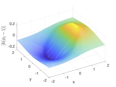
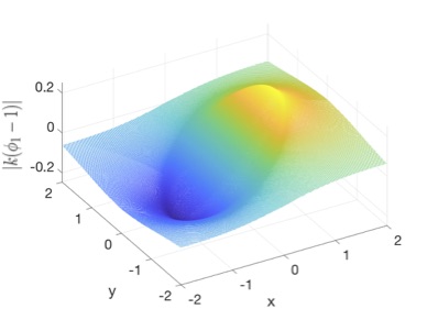
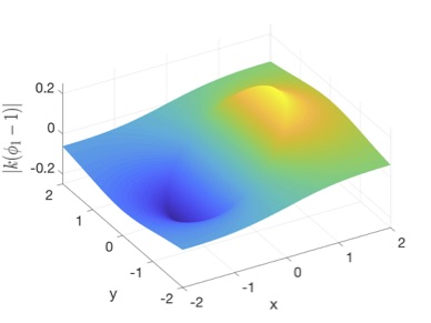
Figure 2. Difference between the solution $\phi_{1}$ for the characteristic function of the disk and 1 multiplied by $k$ for $k=10,100,1000$ from left to right.

In Fig. 3 we show the corresponding plots for $\phi_{2}$. A scaling proportional to $1/k$ as in (5.80) is not obvious for all shown values of $k$. It appears to be realized for the higher values $k=100,1000$.

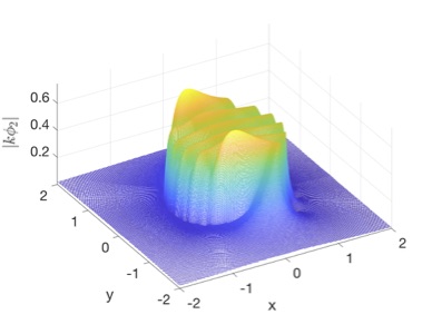
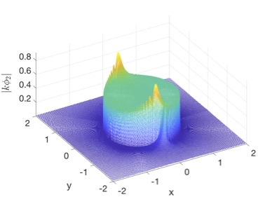
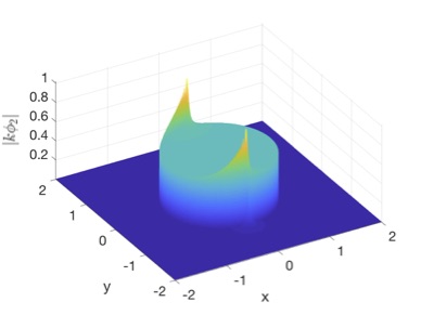
Figure 3. The solution $\phi_{2}$ for the characteristic function of the disk multiplied by $k$ for $k=10,100,1000$ from left to right.

Remark 6.1.

In this section we will always show the pointwise difference between the solution to the d-bar system and various asymptotic formulae for the latter. Note, however, that the asymptotic formulae have been derived for some weighted $L^{2}$ norms. Thus the found differences near the maxima in Fig. 3 will contribute much less in the $L^{2}$ spaces than shown here, where the agreement is already very good.

6.2. Asymptotic formulae

The results of Section 5 imply that $\phi_{1}=1+\mathcal{O}(1/|k|)$ for $|k|\to\infty$, see (5.82). Thus in leading order of $1/k$ the second equation in (1.1) has the approximate solution

$$\tilde{\phi}_{2} =\frac{1}{2\pi}\int_{|w|\leq 1}\frac{\mathrm{e}^{kw-\bar{k}\bar{w}}}{\bar{z}-\bar{w}}d^{2}w=\frac{1}{4\pi k}\int_{0}^{2\pi}\frac{\mathrm{e}^{ke^{-i\varphi}-\bar{k}e^{i\varphi}}-\mathrm{e}^{\bar{k}\bar{z}-kz}}{\bar{z}-e^{-i\varphi}}e^{-i\varphi}d\varphi$$

(6.3) $$=\frac{1}{2\pi}\bar{f}(z,k),$$

i.e. up to a factor the complex conjugate of the integral in 5.5, see also (5.6). We first check how well the function $\tilde{\phi}_{2}$ of (6.3) approximates $\phi_{2}$ for large $k$. Since the integral (6.3) is singular near the boundary and highly oscillatory, it is numerically challenging to evaluate. Therefore we compute it by numerically inverting the $\partial$ operator, the same way as when solving the system (1.1). The difference between $\phi_{2}$ and $\tilde{\phi}_{2}$ can be seen in Fig. 4. It appears to scale as $1/k^{2}$ (see also (5.80)).

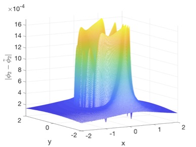
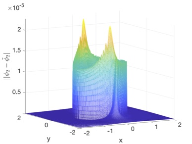
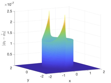
Figure 4. Difference between the solution $\phi_{2}$ for the characteristic function of the disk and $\tilde{\phi}_{2}$ (6.3) for $k=10,100,1000$ from left to right.

The task is thus to compute the function $f(z,k)$ of (5.5) in (6.3) to leading order in $1/|k|$ as in Section 5. We briefly recall the main steps for the example of the characteristic function of the unit disk: We consider the holomorphic extension in $w$ of the integrand by noting that $\bar{w}=1/w$ on the unit circle. Thus we have

(6.4) $$\frac{1}{2\pi}\bar{f}(z,k)=\frac{1}{4\pi ki}\int_{|w|=1}\frac{\mathrm{e}^{k/w-\bar{k}w}}{\bar{z}-w}dw,$$

which was computed in Section 5 asymptotically via a contour deformation and steepest descent techniques. We illustrate the various steps to obtain the asymptotic formula (5.82) for the unit disk below. The interior of the disk $r\leq 1$ and its complement in the complex plane given by $s:=1/r<1$ will be always shown separately in dependence of polar coordinates. The exponent in the integrand of (6.4) has the stationary points $w_{\pm}=\pm i$. The fact that stationary phase approximations are essentially quadratic approximations of the phase means that length scales of order $1/\sqrt{|k|}$ are important. This leads to a natural decomposition of the disk and its complement in the complex plane into zones. Let $r_{k}$ be such that $1-r_{k}=\mathcal{O}(1/\sqrt{|k|})$. We consider the following cases:
I.1 $r<r_{k}$ respectively $s<r_{k}$;
I.2 $r_{k}<r<1$ respectively $r_{k}<s<1$ and $\pi/2+\delta<\varphi<3\pi/2-\delta$ where $\delta>0$ such that $\delta=O(1/\sqrt{|k|})$ or $0\leq\varphi<\pi/2-\delta$ or $3\pi/2+\delta<\varphi<2\pi$;
II. $r_{k}<r<1$ respectively $r_{k}<s<1$ and $\pi/2-\delta\varphi<\pi/2+\delta$ or $3\pi/2-\delta\varphi<3\pi/2+\delta$.

Case I.1

In this case the integral (6.4) can be evaluated with a standard stationary phase approximation, see Section 5. Its leading order contribution in $1/|k|$ to $\phi_{2}$ is with (5.32) and (5.34)

(6.5) $$\begin{cases}\phi_{2}^{I1}&=\frac{e^{kz-\bar{k}\bar{z}}}{4k},\quad|z|\leq 1,\\ \phi_{2}^{I1}&=0,\quad|z|>1,\end{cases}$$

plus corrections of order $O(1/|k|^{3/2})$. In Fig. 5, we show the difference of $\phi_{2}$ and the $\phi_{2}^{I1}$ of (6.5), in the upper row in the interior of the disk, in the lower row in the complement of the disk in the complex plane, both in polar coordinates.

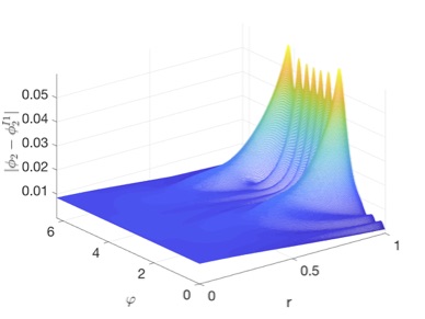
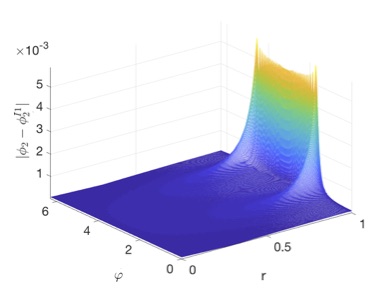
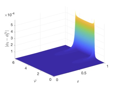
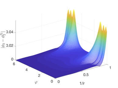
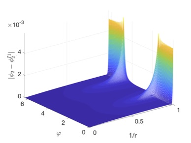
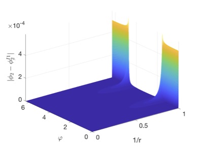
Figure 5. Difference between the solution $\phi_{2}$ for the characteristic function of the disk and $\phi_{2}^{I1}$, in the upper row the interior of the disk, in the lower row the exterior of the disk, both for $k=10,100,1000$ from left to right.

It can be seen that the approximation is as expected not of the wanted order near the rim of the disk. The precise region of applicability of the approximation will be studied below.

Case I.2

Writing $w=\omega\exp(i\psi)$, $\omega>0$, $\psi\in\mathbb{R}$, we get for the exponent in the integral (6.4)

(6.6) $$k\left(w-\frac{1}{w}\right)=k\cos\psi\left(\omega-\frac{1}{\omega}\right)+ik\sin\psi\left(\omega+\frac{1}{\omega}\right).$$

This means we can deform the integration contour in (6.4) as in Fig. 1 for $\pi/2<\psi<3\pi/2$ to a semicircle with $\omega<1$ to get an exponentially small contribution to the integral there for $k$ large. Similarly we deform the contour for $0\leq\psi<\pi/2$ or $3\pi/2<\psi<2\pi$ to a semicircle with $\omega>1$ to get again an exponentially small contribution to the integral. In both cases it is possible to pick up a contribution due to a residue if the pole of the integrand is crossed by the deformation. This gives the following leading order contributions to $\phi_{2}$ in these cases: For $1-r_{k}<r<1$ and $\pi/2<\varphi<3\pi/2$, one has

(6.7) $$\phi_{2}^{I2}=\frac{1}{2k}\left(\mathrm{e}^{kz-\bar{k}\bar{z}}-e^{ke^{i\varphi}/r-\bar{k}e^{-i\varphi}r}\right).$$

The asymptotic formula in the complement of the disk does not change in this case since no residue can be picked up.

If we take this enhanced asymptotic description into account, the upper row of figures in Fig. 5 is now replaced by the figures in Fig. 6. The expected behavior can be seen except in the vicinity of the points $w_{\pm}$. There the difference is still linear in $1/k$.

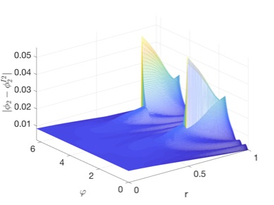
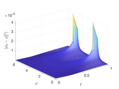
Figure 6. Difference between the solution $\phi_{2}$ for the characteristic function of the disk and $\phi_{2}^{I2}$ from (6.7) at the disk for $k=10,100,1000$ from left to right.

For $\varphi<\pi/2$ or $\varphi>3\pi/2$ there is no contribution due to a residue in the interior of the disk. But in its complement in $\mathbb{C}$, we get

(6.8) $$\phi_{2}^{I2}=\frac{1}{2k}e^{ke^{i\varphi}s-\bar{k}e^{-i\varphi}/s}.$$

This leads to Fig. 7 which shows the same behavior as Fig. 6 for the interior of the disk.

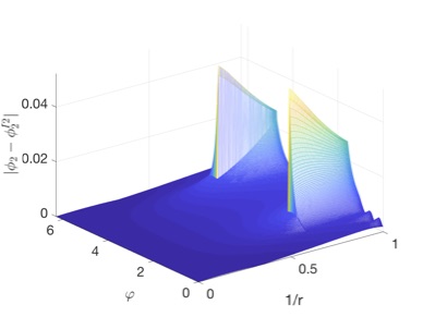
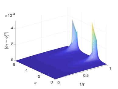
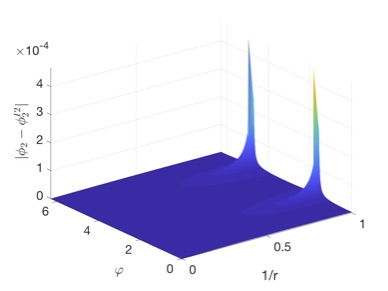
Figure 7. Difference between the solution $\phi_{2}$ for the characteristic function of the disk and $\phi_{2}^{I2}$ from (6.8) for the exterior of the disk for $k=10,100,1000$ from left to right.

Case II

We now address the case that $z$ is close to the stationary points $w_{\pm}$ of the exponent in (6.4), $|z-w_{\pm}|=\mathcal{O}(1/\sqrt{|k|})$. In Section 5 a quadratic approximation to the exponent was considered. We put $w=w_{\pm}+\xi$ and get for $|\xi|\ll 1$ for the exponent $w-1/w=\pm 2i(1-\xi^{2}/2)+\mathcal{O}(|\xi|^{3})$. As the integration path we use the line $\xi=a_{\pm}\eta$, where $\eta\in\mathbb{R}$ and where $a_{\pm}=\sqrt{w_{\pm}/(2k)}$ in order to get an integrand exponentially decaying on the integration path. We consider the function (5.59)

(6.9) $$G(z):=\int_{-\infty}^{\infty}\frac{e^{-t^{2}/2}}{z-t}dt.$$

Note that the function $G$ is not uniquely defined by (6.9) because of the pole on the real axis which is also the integration contour. We denote by $G_{r}(z)$ the analytical continuation to the whole complex plane of the function obtained by computing $G$ in standard way for $\Im z>0$, and $G_{l}(z)$ for $\Im z<0$.

Numerically these functions are computed on the parallels to the real axis going through $-i(\Im z+3)$ for $G_{l}$ and $i(\Im z+3)$ for $G_{r}$. On these lines, the integrand is approximated via a truncated Fourier series on a sufficiently large period, $t\in L[-\pi,\pi]$ (we use $L=10$ in the following). We compute in $t$ the standard discrete Fourier transform, i.e., sample the integrand on $t_{n}=L(-\pi+nh)$, $n=1,\ldots,N$, where $N\in\mathbb{N}$ is the number of collocation points and where $h=2\pi/N$. The integral in (6.9) is the Fourier coefficient with index 0 of the discrete Fourier transform of this function, i.e., simply the sum over $n$ of the integrand in (6.9) sampled at the collocation points $t_{n}$. Since this is one of the coefficients of the discrete Fourier transform, the resulting numerical method is a so-called spectral method. This means the numerical error in approximating the integrand (which is analytic on the chosen integration path) decreases exponentially with $N$. The numerical accuracy is controlled via the decay of the discrete Fourier coefficients which can be computed with a fast Fourier transform. We show both functions $G_{l,r}$ in Fig. 8. The difference between the functions on the real axis is according to (5.60) equal to $2\pi i\exp(-x^{2}/2)$. The functions satisfy the symmetry relation

(6.10) $$G_{l}(\bar{z})=\overline{G_{r}(z)}.$$

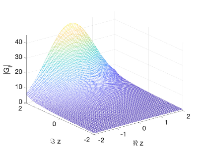
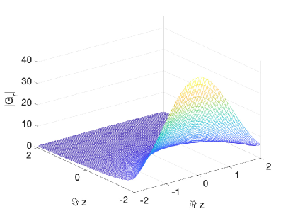
Figure 8. Moduli of the function $G_{l}$ on the left and $G_{r}$ on the right.

Thus we get for the integral (6.4)

(6.11) $$\begin{split}\frac{\bar{f}(k,z)}{2\pi}\approx&\frac{e^{k(1/w_{\pm}-w_{\pm})}}{4\pi ik}\int_{\xi_{1}}^{\xi_{2}}\frac{e^{-k\xi^{2}/w_{\pm}}}{\bar{z}-w_{\pm}-\xi}d\xi\\ &=\frac{e^{k(1/w_{\pm}-w_{\pm})}}{4\pi ik}\int_{\eta_{1}}^{\eta_{2}}\frac{e^{-\eta^{2}/2}}{(\bar{z}-w_{\pm})/a_{\pm}-\eta}d\eta\end{split}.$$

Since the integrand is exponentially decaying, we finally arrive for $|\bar{z}+i|\leq C/|k|$, where $C$ is some positive constant, at the approximations for the interior of the disk

(6.12) $$\phi_{2}^{II}=\begin{cases}\frac{e^{2ik}}{4\pi ik}G_{r}\left(\frac{\bar{z}+i}{a_{-}}\right)+\frac{1}{2k}\left(\mathrm{e}^{kz-\bar{k}\bar{z}}-e^{ke^{i\varphi}/r-\bar{k}e^{-i\varphi}r}\right),&\Im z+1\leq\Re z\\ \frac{e^{2ik}}{4\pi ik}G_{l}\left(\frac{\bar{z}+i}{a_{-}}\right)+\frac{e^{kz-\bar{k}\bar{z}}}{2k},&\Im z+1>\Re z\end{cases}$$

and

(6.13) $$\phi_{2}^{II}=\begin{cases}\frac{e^{2ik}}{4\pi ik}G_{l}\left(\frac{\bar{z}+i}{a_{-}}\right),&\Im z+1\leq\Re z\\ \frac{e^{2ik}}{4\pi ik}G_{r}\left(\frac{\bar{z}+i}{a_{-}}\right)-\frac{1}{2k}e^{ke^{i\varphi}/r-\bar{k}e^{-i\varphi}r},&\Im z+1>\Re z\end{cases}$$

in the exterior of the disk. Analogous formulae hold for $|\bar{z}-i|\leq C/|k|$.

In Fig, 9 we show the effect of all above asymptotic descriptions for the interior of the disk. Approximation (6.12) is applied for $|\bar{z}-w_{\pm}|<C/\sqrt{|k|}$ for $C=1$, see (5.32). It can be seen that the approximation is excellent near the points $w_{\pm}$, the error is largest near these points where the approximation of case I is applied.

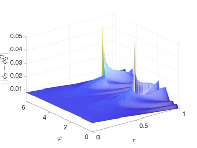
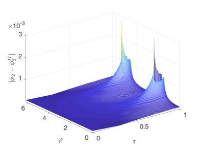
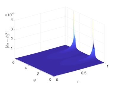
Figure 9. Difference between the solution $\phi_{2}$ for the characteristic function of the disk and $\phi_{2}^{II}$ from (6.12) for the interior of the disk for $k=10,100,1000$ from left to right ($C=1$).

Since the error near the points $w_{\pm}$ in Fig. 9 is largest where the approximation (6.12) is not applied, it appears reasonable that larger values of the constant $C$ should be considered. The asymptotic formulae of section 5 do not fix this constant. Since we consider values of $k$ as low as 10, we cannot choose $C$ too large since otherwise the regions in the vicinity of $w_{\pm}$ would overlap. In Fig. 10 we show the same differences as in Fig. 9, but this time for $C=4$. The overall error is considerably lower in this case than for $C=1$ and is still dominated by the regions $|z-w_{\pm}|>C/\sqrt{k}$. For large $|k|$ one could optimize the choice of $C$, but this is beyond the goal of this paper.

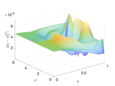
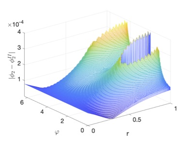
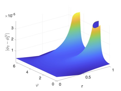
Figure 10. Difference between the solution $\phi_{2}$ for the characteristic function of the disk and $\phi_{2}^{II}$ from (6.12) for the interior of the disk for $k=10,100,1000$ from left to right ($C=4$).

A similar behavior can be seen in the complement of the disk in the complex plane in Fig. 11.

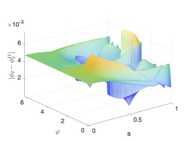
Figure 11. Difference between the solution $\phi_{2}$ for the characteristic function of the disk and $\phi_{2,e}^{III}$ from (6.12) for the exterior of the disk for $k=10,100,1000$ from left to right.

6.3. Reflection coefficient

As stated in the introduction, the main quantity of interest in an inverse scattering approach to DS II is the reflection coefficient (1.8) which plays here the role of the Fourier transform for linear equations and is the angle in terms of action-angle variables.

The analysis in Section 5 has shown that the function $\phi_{1}$ is given in leading order by the expresssion (5.82). In the case of the unit disk we are interested in here, this takes the form

(6.14) $$\tilde{\phi}_{1}=1+\frac{\bar{z}}{4k}$$

for $|k|\to\infty$ ($\phi_{1}=\tilde{\phi}_{1}+\mathcal{O}(|k|^{-3/2}|k|)$). In the exterior of the disk, the function is holomorphic and tends to 1 at infinity. Since it is continuous at the disk, we have $\tilde{\phi}_{1}=1+\frac{1}{4kz}$ for $|z|>1$.

We show in Fig. 12 the difference between $\phi_{1}$ and $\tilde{\phi}_{1}$. This difference is largest near the rim of the disk, but appears to be of order $1/k^{2}$.

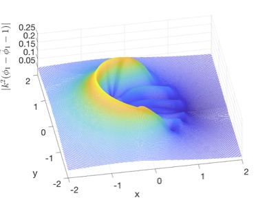
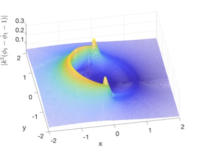
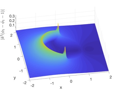
Figure 12. Difference between the solution $\phi_{1}$ for the characteristic function of the disk and $1+\frac{\bar{z}}{4k}$ multiplied by $k^{2}$ for $k=10,100,1000$ from left to right.

The reflection coefficient is given via $\bar{R}(k)=2\lim_{z\to\infty}\bar{z}\phi_{2}$, i.e.,

(6.15) $$\bar{R}=\frac{2}{\pi}\int_{|z|\leq 1}\mathrm{e}^{kw-\bar{k}\bar{w}}\phi_{1}d^{2}w\approx\frac{2}{\pi}\int_{|z|\leq 1}\mathrm{e}^{kw-\bar{k}\bar{w}}\left(1+\frac{\bar{w}}{4k}\right)d^{2}w.$$

The reflection coefficient is real in this case. Note that the error term in (5.82) can contribute in the oscillatory integral (6.15) in the order we would like to study. If we conjecture that this is not the case, then the integral (6.15) can be computed once more with a stationary phase approximation (of higher order), which allows us to study higher order terms. After some calculation we get

(6.16) $$R\approx R_{asym}:=\frac{1}{\sqrt{\pi k^{3}}}\left(\sin(2k-\pi/4)-\frac{5}{16k}\cos(2k-\pi/4)\right).$$

We show the reflection coefficient in Fig. 13 on the left in blue. The asymptotic formula for the coefficient shown in the same figure in red agrees so well with the coefficient even for values of $k$ of the order 10 that we show on the right of the same figure the difference between $R$ and the asymptotic formula (6.16) multiplied with $k^{7/2}$. This indicates that the corrections to formula (6.16) are of the order $k^{-7/2}$, but that this asymptotic regime is only reached for larger values of $k$ than shown.

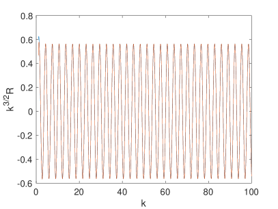
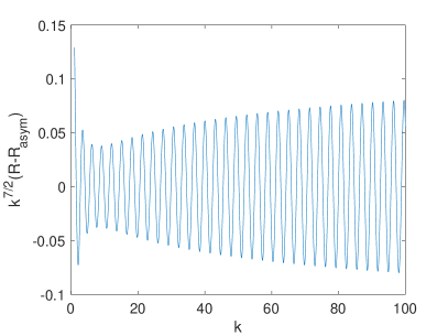
Figure 13. Reflection coefficient for the characteristic function of the disk, on the left $R$ in blue and $R_{asym}$ from (6.16) in red, both multiplied with $k^{3/2}$, on the right the difference between both multiplied with $k^{7/2}$.

An error term of the order of $|k|^{-7/2}$ implies that for $k=1000$, which can be reached numerically at least with an accuracy of the order of $10^{-11}$ as discussed in [18], will be of the order $10^{-11}$. This means that the asymptotic formula for the reflection coefficient is applicable already for values of the spectral parameter $k$ where the numerical approach can be applied. In other words, in the example of the characteristic function of the disk, a hybrid approach of a numerical approach for $|k|<k_{0}$ with $k_{0}\sim 10^{3}$ combined with the asymptotic formula (6.16) for $|k|>k_{0}$ allows for a computation of the reflection coefficient for all $k\in\mathbb{C}$ with an accuracy of $10^{-11}$ and better.

References

- [1] M.J. Ablowitz, A.S. Fokas, On the inverse scattering transform of multidimensional nonlinear evolution equations related to first order systems in the plane, J. Math Phys. 25 no 8 (1984), 2494-2505.
- [2] Assainova, O., Klein, C., McLaughlin, K. D. and Miller, P. D., A Study of the Direct Spectral Transform for the Defocusing Davey-Stewartson II Equation the Semiclassical Limit. Comm. Pure Appl. Math., 72: 1474-1547 (2019).
- [3] R. Beals and R. Coifman, Multidimensional inverse scattering and nonlinear PDE Proc. Symp. Pure Math. (Providence: American Mathematical Society) 43, 45-70 (1985)
- [4] R.M. Brown, Estimates for the scattering map associated with a two-dimensional first-order system. J. Nonlinear Sci. 11, no. 6, 459-471 (2001)
- [5] R. Brown and P. Perry, Soliton solutions and their (in)stability for the focusing Davey-Stewartson II equation, Nonlinearity 31(9) 4290 doi.org/10.1088/1361-6544/aacc46 (2018)
- [6] R.M. Brown, G.A. Uhlmann, Communications in partial differential equations 22 (5-6), 1009-1027 (1997)
- [7] A.P. Calderón, On inverse boundary value problem. Seminar on Numerical Analysis and its Applications to Continuum Physics (Rio de Janeiro, 1980) pp 65-73 (Soc. Brasil. Mat.)
- [8] M. Dimassi, J. Sjöstrand, Spectral asymptotics in the semi-classical limit, London Math. Soc. Lecture Notes Series 269, Cambridge University Press 1999.
- [9] A.S. Fokas, On the Inverse Scattering of First Order Systems in the Plane Related to Nonlinear Multidimensional Equations, Phys. Rev. Lett. 51, 3-6 (1983)
- [10] A.S. Fokas and M.J. Ablowitz, On a Method of Solution for a Class of Multi-Dimensional Nonlinear Evolution Equations, Phys. Rev. Lett. 51, 7-10 (1983)
- [11] C. Kenig, J. Sjöstrand, G. Uhlmann. The Calderón problem with partial data. Annals of Mathematics 165 (2007), 567-591.
- [12] A. G. Gurevich, L. P. Pitaevskii, Non stationary structure of a collisionless shock waves, JEPT Letters 17 (1973), 193-195.
- [13] L. Hörmander, An introduction to complex analysis in several variables, Third edition, North-Holland Mathematical Library 7 (North-Holland Publishing Co., Amsterdam, 1990)
- [14] C. Klein and K. McLaughlin, Spectral approach to D-bar problems, Comm. Pure Appl. Math., DOI: 10.1002/cpa.21684 (2017)
- [15] C. Klein, K. McLaughlin and N. Stoilov, Spectral approach to semi-classical d-bar problems with Schwartz class potentials, Physica D: Nonlinear Phenomena DOI: 10.1016/j.physd.2019.05.006 (2019)
- [16] C. Klein and K. Roidot, Numerical Study of the semiclassical limit of the Davey-Stewartson II equations, Nonlinearity 27, 2177-2214 (2014).
- [17] C. Klein, J.-C. Saut, IST versus PDE: a comparative study. Hamiltonian partial differential equations and applications, 383-449, Fields Inst. Commun., 75, Fields Inst. Res. Math. Sci., Toronto, ON, (2015)
- [18] C. Klein and N. Stoilov, A numerical study of blow-up mechanisms for Davey-Stewartson II systems, Stud. Appl. Math., DOI : 10.1111/sapm.12214 (2018)
- [19] C. Klein and N. Stoilov, Numerical scattering for the defocusing Davey-Stewartson II equation for initial data with compact support, Nonlinearity 32 (2019) 4258-4280
- [20] K. Knudsen, J. L. Mueller, S. Siltanen. Numerical solution method for the d-bar equation in the plane. J. Comput. Phys. 198 no. 2, 500-517 (2004).
- [21] J.L. Mueller and S. Siltanen. Linear and Nonlinear Inverse Problems with Practical Applications, SIAM, 2012.
- [22] P. Muller, D. Isaacson, J. Newell, and G. Saulnier. A Finite Difference Solver for the D-bar Equation. Proceedings of the 15th International Conference on Biomedical Applications of Electrical Impedance Tomography, Gananoque, Canada, 2014.
- [23] A. I. Nachman, I. Regev, and D. I. Tataru, A nonlinear Plancherel theorem with applications to global well-posedness for the defocusing Davey-Stewartson equation and to the inverse boundary value problem of Calderon, arXiv:1708.04759, 2017.
- [24] P. Perry. Global well-posedness and long-time asymptotics for the defocussing Davey-Stewartson II equation in . Preprint available at arxiv.org/pdf/1110.5589v2.pdf.
- [25] L.Y. Sung, An inverse scattering transform for the Davey-Stewartson equations. I, J. Math. Anal. Appl. 183 (1) (1994), 121-154.
- [26] L.Y. Sung, An inverse scattering transform for the Davey-Stewartson equations. II, J. Math. Anal. Appl. 183 (2) (1994), 289-325.
- [27] L.Y. Sung, An inverse scattering transform for the Davey-Stewartson equations. III, J. Math. Anal. Appl. 183 , 477-494 (1994)
- [28] G. Uhlmann. Electrical impedance tomography and Calderón’s problem. Inverse Problems, 25(12):123011, 2009.