Few-particle scattering from localized quantum systems in spatially structured bosonic baths

Rahul Trivedi Affiliation: Max Planck Institut für Quantenoptik, Garching bei München, 85748, Germany. Email: rahul.trivedi@mpq.mpg.de Thanks: Source code for the numerical simulations in this paper is available here    Kevin Fischer Affiliation: Stanford University, Stanford, CA, 94305, USA.    Shanhui Fan Affiliation: Stanford University, Stanford, CA, 94305, USA.    Jelena Vuckovic Affiliation: Stanford University, Stanford, CA, 94305, USA.
Abstract

Understanding the dynamics of localized quantum systems embedded in engineered bosonic environments is a central problem in quantum optics and open quantum system theory. We present a formalism for studying few-particle scattering in a localized quantum system interacting with an bosonic bath described by an inhomogeneous wave-equation. In particular, we provide exact relationships between the quantum scattering matrix of this interacting system and frequency domain solutions of the inhomogeneous wave-equation thus providing access to the spatial distribution of the scattered few-particle wave-packet. The formalism developed in this paper paves the way to computationally understanding the impact of structured media on the scattering properties of localized quantum systems embedded in them without simplifying assumptions on the physics of the structured media.

I Introduction

Non-classical light sources lodahl2015interfacing; ding2016demand; michler; senellart2017high; zhang2018strongly; kok2007linear; o2009photonic; roy2017colloquium; reiserer2015cavity; duan2010colloquium; sangouard2011quantum; nemoto2014photonic are an essential resource in all optical quantum information processing and communication systems. Traditionally, such light sources have been designed by interfacing localized quantum systems (quantum dots, color centers etc.) with a bosonic bath (an electromagnetic structure such as an optical fiber, waveguide or optical cavity). The localized quantum system can modify the statistics and the entanglement structure of an incoming state propagating in the bosonic bath englund2005controlling; daveau2017efficient; pelton2002efficient; he2013demand; fischer2017signatures; hanschke2018quantum; metcalfe2010resolved; miao2019electrically; lukin2020spectrally. This has opened up the possibility of generating high-fidelity single photon sources he2013demand; wang2019towards, photon pair sources li2004all; harder2013optimized as well as high-dimensional entangled photon states pichler2016photonic; xu2018generate by engineering both the bath as well as the Hamiltonian of the localized quantum systems.

From a theoretical standpoint, a quantitative theory of the dynamics and scattering properties of this coupled system is required for designing any of the above-mentioned applications. If only the dynamics of the localized system is of interest, the usual approach is to trace out the Hilbert space of the bath to obtain a master equation for the density operator of the localized system carmichael2009open; gardiner2004quantum. While traditionally the master equation is formulated for a one-dimensional homogeneous bath gardiner2004quantum, it is easily extended to cases where the bath is described by an inhomogeneous 3D wave-equation asenjo2017atom; dung2002resonant. However, a significant drawback of the master equation formalism is that it is not amenable to computing the state of the bath, although recent works have attempted to resolve this problem for 1D homogeneous baths kiilerich2019input.

An alternative set of computational and analytical tools which allow us to calculate the bath’s quantum state is provided by scattering theory taylor2006scattering. Here, the localized system is treated as a scatterer for the quantum states that otherwise propagate in the bath. Significant progress has been made on scattering theory for systems where a modal decomposition of the bosonic bath is easily accessible. In particular, there has been great success in developing techniques for analyzing the scattering matrices of the localized quantum system when the electromagnetic structure is a photonic waveguide fan2010input; xu2013analytic; xu2015input; trivedi2018few; trivedi2021optimal; fischer2017scattering; shi2015multiphoton; caneva2015quantum, a cavity haroche1993cavity; trivedi2019photon; shi2013two or a network of these components. There has also been progress towards understanding the interaction of localized quantum systems with 3D homogeneous baths liu2016quantum and periodically structured baths orenstein2020two. Computing the scattering of few-photon states in systems where the bosonic bath is describable as arbitrary spatially varying permittivity distributions remains an open problem. Such a framework, if it exists, can enable both analysis and design of more complex quantum photonic devices similar to how computational electromagnetic methods capable of simulating arbitrary permittivity distributions revolutionized the design of classical photonic devices miller1988selective; molesky2018inverse.

In this paper, we present a framework for exactly calculating the scattering matrix of a localized quantum system interacting with a bosonic bath whose dynamics are described by an inhomogeneous wave equation. There are two key ingredients that go towards making this framework possible —

  1. 1.

    A second quantized description of the inhomogeneous bosonic bath in terms of both Langevin noise operators and plane-wave annihilation operators (Section II). Here, we build upon the formalism presented in Refs. dung1998three; gruner1996green for quantizing lossy frequency-dependent and inhomogeneous electromagnetic environments.

  2. 2.

    Calculation of few-particle scattering matrices that builds on this second quantized description (Section III). We express the spatial and spectral dependence of the few-particle scattering matrices in terms of two quantities — first, the frequency-domain solutions of the inhomogeneous wave-equation describing the bath dynamics and second, the time-ordered expectations of the localized system operators (Section III). While our general approach is applicable to arbitrary localized systems, we provide exact expressions for the single and two-particle scattering matrices for the paradigmatic example of a two-level localized system.

II Quantization of an inhomogeneous bosonic bath
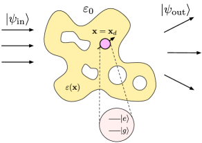
Figure 1: Schematic. A localized two-level system interacting with an inhomogeneous bosonic bath described by a permittivity distribution ε(𝐱)\varepsilon(\mathbf{x}) which is asymptotically homogeneous (ε(𝐱)ε0\varepsilon(\mathbf{x})\to\varepsilon_{0} as |𝐱||\mathbf{x}|\to\infty). An incident few-particle state |ψin\ket{\psi_{\text{in}}} propagates through the inhomogeneous bath and scatters off the localized system to produce an outgoing few-particle state |ψout\ket{\psi_{\text{out}}}.

Figure 1 schematically depicts the systems under consideration comprising of a localized quantum system interacting with an inhomogeneous bosonic bath. We assume that the bosonic bath is classically described by the inhomogenous wave-equation

2ψ(𝐱,t)=ε(𝐱)2t2ψ(𝐱,t),\nabla^{2}\psi(\mathbf{x},t)=\varepsilon(\mathbf{x})\frac{\partial^{2}}{\partial t^{2}}\psi(\mathbf{x},t), (1)

where ψ(𝐱,t)\psi(\mathbf{x},t) is the time-dependent field variable and ε(𝐱)\varepsilon(\mathbf{x}) is the permittivity distribution describing the inhomogeneity in the bath. While we restrict ourselves to a simple scalar wave-equation model in this paper, an extension to a full vector-wave equation model is also possible. Furthermore, we will assume that the bosonic bath in isolation is lossless and consequently the permittivity distribution ε(𝐱)\varepsilon(\mathbf{x}) is real and positive. Furthermore, we assume that the inhomogeneous media is embedded in a background homogeneous media with permittivity ε0\varepsilon_{0} i.e. ε(𝐱)ε0\varepsilon(\mathbf{x})\to\varepsilon_{0} as |𝐱||\mathbf{x}|\to\infty.

II.1 First quantization

A quantum theory for such a bosonic bath can easily be developed by applying Dirac’s quantization weinberg1995quantum procedure on its classical Lagrangian bath[ψ]\mathcal{L}_{\text{bath}}[\psi]

bath[ψ]=123(ε(𝐱)|ψ(𝐱,t)t|2|ψ(𝐱,t)|2)d3𝐱.\mathcal{L}_{\text{bath}}[\psi]=\frac{1}{2}\int_{\mathbb{R}^{3}}\bigg(\varepsilon(\mathbf{x})\bigg|\frac{\partial\psi(\mathbf{x},t)}{\partial t}\bigg|^{2}-|\nabla\psi(\mathbf{x},t)|^{2}\bigg)d^{3}\mathbf{x}. (2)

From this lagrangian, the canonically conjugate field to ψ(𝐱,t)\psi(\mathbf{x},t) is easily identified to be

π(𝐱,t)=ε(𝐱)ψ(𝐱,t)t.\displaystyle\pi(\mathbf{x},t)=\varepsilon(\mathbf{x})\frac{\partial\psi(\mathbf{x},t)}{\partial t}. (3)

Dirac’s quantization then promotes both of these fields to operators, ψ(𝐱)\psi(\mathbf{x}) and π(𝐱)\pi(\mathbf{x}), with commutator [ψ(𝐱),π(𝐱)]=iδ3(𝐱𝐱)[\psi(\mathbf{x}),\pi(\mathbf{x}^{\prime})]=i\delta^{3}(\mathbf{x}-\mathbf{x}^{\prime}). Furthermore, the dynamics of the quantum state of the bath is governed by the Hamiltonian

Hbath=3(π2(𝐱)2ε(𝐱)+12|ψ(𝐱)|2)d3𝐱\displaystyle H_{\text{bath}}=\int_{\mathbb{R}^{3}}\bigg(\frac{\pi^{2}(\mathbf{x})}{2\varepsilon(\mathbf{x})}+\frac{1}{2}|\nabla\psi(\mathbf{x})|^{2}\bigg)d^{3}\mathbf{x} (4)

It can be readily verified that the Heisenberg equations of motion for the operators ψ(𝐱)\psi(\mathbf{x}) and π(𝐱)\pi(\mathbf{x}) reproduce the equations of motion for the classical fields as given by Eqs. 1 and 3.

II.2 Second quantization

While the first quantized description provides a complete quantum theory for the bosonic bath, it does not allow for an easy and physically meaningful description of incident and scattered quantum states. It is, therefore, of interest to perform second quantization and introduce particle annihilation and creation operators. We accomplish a second quantization of an inhomogeneous bosonic bath in two steps. First, we consider a more general case of lossy inhomogeneous media and introduce a second quantization based on Langevin noise formalism. Second, we treating lossless inhomogeneous media as a limiting case of lossy inhomogeneous media, we construct a second quantization in which an annihilation operator is associated with each possible plane-wave incident on the inhomogeneous media.

II.2.1 Langevin noise formalism

In this subsection, we build upon the formalism introduced in Refs. dung1998three; gruner1996green which quantize the wave-equation in lossy inhomogeneous Kramer-Kronig dielectrics using a Langevin noise-operator approach. However, since we are fundamentally interested in lossless inhomogeneous baths, to make use of this formalism we fictitiously introduce loss in the bosonic bath, and consider a frequency-dependent permittivity distribution εα(𝐱,ω)\varepsilon_{\alpha}(\mathbf{x},\omega) given by

εα(𝐱,ω)=ε(𝐱)+iα(ω),\displaystyle\varepsilon_{\alpha}(\mathbf{x},\omega)=\varepsilon(\mathbf{x})+i\alpha(\omega), (5)

where α(ω)>0\alpha(\omega)>0 is the loss in the permittivity distribution. For simplicity, we assume the loss to be position independent — the permittivity distribution εα(𝐱,ω)\varepsilon_{\alpha}(\mathbf{x},\omega) is thus that of a lossy inhomogeneous permittivity distribution in a homogeneous background with permittivity ε0+iα(ω)\varepsilon_{0}+i\alpha(\omega). While we could work with a position dependent loss as well, since the objective is to study the limiting case of a lossless permittivity distribution, the position dependence of the loss does not matter.

With the introduction of this loss, following Ref. dung1998three we introduce a bosonic noise operator ϕα(𝐱,ω)\phi_{\alpha}(\mathbf{x},\omega) for every position 𝐱\mathbf{x} and for every frequency ω>0\omega>0 which satisfy [ϕα(𝐱,ω),ϕα(𝐱,ω)]=δ3(𝐱𝐱)δ(ωω)[\phi_{\alpha}(\mathbf{x},\omega),\phi^{\dagger}_{\alpha}(\mathbf{x}^{\prime},\omega^{\prime})]=\delta^{3}(\mathbf{x}-\mathbf{x}^{\prime})\delta(\omega-\omega^{\prime}). Furthermore, the bath’s Hamiltonian is expressible as11 1 We use the notation that +:=[0,)\mathbb{R}^{+}:=[0,\infty),

Hbath=𝐱3ω+ωϕα(𝐱,ω)ϕα(𝐱,ω)d3𝐱𝑑ω.H_{\text{bath}}=\int_{\begin{subarray}{c}\mathbf{x}\in\mathbb{R}^{3}\\ \omega\in\mathbb{R}^{+}\end{subarray}}\omega\phi^{\dagger}_{\alpha}(\mathbf{x},\omega)\phi_{\alpha}(\mathbf{x},\omega)\ d^{3}\mathbf{x}\ d\omega. (6)

We define the single-frequency field operator in the presence of loss, ψα(𝐱,ω)\psi_{\alpha}(\mathbf{x},\omega), in terms of the noise operators ϕα(𝐱,ω)\phi_{\alpha}(\mathbf{x},\omega) by

ψα(𝐱,ω)=(ω2α(ω)π)1/2×\displaystyle\psi_{\alpha}(\mathbf{x},\omega)=\bigg(\frac{\omega^{2}\alpha(\omega)}{\pi}\bigg)^{1/2}\times
𝐱3Gα(𝐱,𝐱,ω)ϕα(𝐱,ω)d3𝐱𝑑ω,\displaystyle\qquad\int_{\mathbf{x}^{\prime}\in\mathbb{R}^{3}}\text{G}_{\alpha}(\mathbf{x},\mathbf{x}^{\prime};\omega)\phi_{\alpha}(\mathbf{x}^{\prime},\omega)d^{3}\mathbf{x}^{\prime}d\omega, (7)

where Gα(𝐱,𝐱,ω)\text{G}_{\alpha}(\mathbf{x},\mathbf{x}^{\prime};\omega) is the Green’s function corresponding to the lossy inhomogeneous bath, which is obtained by solving the partial differential equation

[𝐱2+ω2εα(𝐱,ω)]Gα(𝐱,𝐱,ω)=δ3(𝐱𝐱).\big[\nabla_{\mathbf{x}}^{2}+\omega^{2}\varepsilon_{\alpha}(\mathbf{x},\omega)\big]\text{G}_{\alpha}(\mathbf{x},\mathbf{x}^{\prime};\omega)=\delta^{3}(\mathbf{x}-\mathbf{x}^{\prime}). (8)

under the boundary condition that Gα(𝐱,𝐱,ω)\text{G}_{\alpha}(\mathbf{x},\mathbf{x}^{\prime};\omega) is an outgoing wave as |𝐱||\mathbf{x}|\to\infty. We point out that since Im[εα(𝐱,ω)]=α(ω)>0\text{Im}[\varepsilon_{\alpha}(\mathbf{x},\omega)]=\alpha(\omega)>0, this boundary condition also implies that Gα(𝐱,𝐱,ω)\text{G}_{\alpha}(\mathbf{x},\mathbf{x}^{\prime};\omega) decays exponentially with |𝐱||\mathbf{x}| as |𝐱||\mathbf{x}|\to\infty. The field operators in the presence of loss, ψα(𝐱)\psi_{\alpha}(\mathbf{x}) and πα(𝐱)\pi_{\alpha}(\mathbf{x}), are related to the single-frequency field operator via

ψα(𝐱)=iω+(ψα(𝐱,ω)ψα(𝐱,ω))𝑑ω,\displaystyle\psi_{\alpha}(\mathbf{x})=i\int_{\omega\in\mathbb{R}^{+}}\big(\psi_{\alpha}(\mathbf{x},\omega)-\psi_{\alpha}^{\dagger}(\mathbf{x},\omega)\big)d\omega, (9a)
πα(𝐱)=ε(𝐱)ω+ω(ψα(𝐱,ω)ψα(𝐱,ω))𝑑ω.\displaystyle\pi_{\alpha}(\mathbf{x})=\varepsilon(\mathbf{x})\int_{\omega\in\mathbb{R}^{+}}\omega\big(\psi_{\alpha}(\mathbf{x},\omega)-\psi_{\alpha}^{\dagger}(\mathbf{x},\omega)\big)d\omega. (9b)

It is shown in appendix A that the single-frequency field operator ψα(𝐱,ω)\psi_{\alpha}(\mathbf{x},\omega) has the commutator [ψα(𝐱,ω),ψα(𝐱,ω)]=δ(ωω)Im[Gα(𝐱,𝐱;ω)]/2π[\psi_{\alpha}(\mathbf{x},\omega),\psi_{\alpha}^{\dagger}(\mathbf{x}^{\prime},\omega^{\prime})]=-{\delta(\omega-\omega^{\prime})}\text{Im}\big[\text{G}_{\alpha}(\mathbf{x},\mathbf{x}^{\prime};\omega)\big]/{2\pi}. Furthermore, this implies that the operators ψα(𝐱)\psi_{\alpha}(\mathbf{x}) and πα(𝐱)\pi_{\alpha}(\mathbf{x}) satisfy the canonical commutation relations [ψα(𝐱),πα(𝐲)]=iδ3(𝐱𝐲)[\psi_{\alpha}(\mathbf{x}),\pi_{\alpha}(\mathbf{y})]=i\delta^{3}(\mathbf{x}-\mathbf{y}). Finally, we point out the field operators for a lossless bosonic bath, ψ(𝐱,ω),ψ(𝐱),π(𝐱)\psi(\mathbf{x},\omega),\psi(\mathbf{x}),\pi(\mathbf{x}), can be constructed from the operators ψα(𝐱,ω),ψα(𝐱),πα(𝐱)\psi_{\alpha}(\mathbf{x},\omega),\psi_{\alpha}(\mathbf{x}),\pi_{\alpha}(\mathbf{x}) by taking α(ω)0\alpha(\omega)\to 0. Since limα(ω)0Im[Gα(𝐱,𝐱,ω)]\lim_{\alpha(\omega)\to 0}\text{Im}\big[\text{G}_{\alpha}(\mathbf{x},\mathbf{x}^{\prime};\omega)] exists and is well defined, this immediately implies the following commutator for the single-frequency field operator

[ψ(𝐱,ω),ψ(𝐱,ω)]=δ(ωω)2πIm[G(𝐱,𝐱,ω)],\displaystyle[\psi(\mathbf{x},\omega),\psi^{\dagger}(\mathbf{x}^{\prime},\omega^{\prime})]=-\frac{\delta(\omega-\omega^{\prime})}{2\pi}\text{Im}\big[\text{G}(\mathbf{x},\mathbf{x}^{\prime};\omega)\big], (10)

and the canonical commutation relation, [ψ(𝐱),π(𝐱)]=iδ3(𝐱𝐱)[\psi(\mathbf{x}),\pi(\mathbf{x}^{\prime})]=i\delta^{3}(\mathbf{x}-\mathbf{x}^{\prime}), holds between the full field operators ψ(𝐱)\psi(\mathbf{x}) and π(𝐱)\pi(\mathbf{x}).

II.2.2 Second quantization with plane-wave operators

Since the physics of an inhomogeneous bath can fundamentally be captured by the fields scattered from the inhomogeneity when excited by incident plane-waves, we seek its second quantized description in terms of incident plane-wave annihilation operators. This can be derived from the noise-operator description by taking the limit of α(ω)0\alpha(\omega)\to 0. In order to take this limit, we express the Green’s function Gα(𝐱,𝐱,ω)\text{G}_{\alpha}(\mathbf{x},\mathbf{x}^{\prime};\omega) as

Gα(𝐱,𝐱,ω)=\displaystyle\text{G}_{\alpha}(\mathbf{x},\mathbf{x}^{\prime};\omega)=
Gα0(𝐱,𝐱,ω)+3Sα(𝐱,𝐲,ω)Gα0(𝐲,𝐱,ω)d3𝐲,\displaystyle\quad\text{G}_{\alpha}^{0}(\mathbf{x},\mathbf{x}^{\prime};\omega)+\int_{\mathbb{R}^{3}}\text{S}_{\alpha}(\mathbf{x},\mathbf{y};\omega)\text{G}_{\alpha}^{0}(\mathbf{y},\mathbf{x}^{\prime};\omega)d^{3}\mathbf{y}, (11)

where Gα(𝐱,𝐱,ω)\text{G}_{\alpha}(\mathbf{x},\mathbf{x}^{\prime};\omega) is the Green’s function corresponding to the (lossy) background i.e. it is the solution of the partial differential equation

[𝐱2+ω2(ε0+iα(ω))]Gα0(𝐱,𝐱,ω)=δ3(𝐱𝐱),\displaystyle\big[\nabla_{\mathbf{x}}^{2}+\omega^{2}(\varepsilon_{0}+i\alpha(\omega))\big]\text{G}_{\alpha}^{0}(\mathbf{x},\mathbf{x}^{\prime};\omega)=\delta^{3}(\mathbf{x}-\mathbf{x}^{\prime}), (12)

with the boundary condition that Gα0(𝐱,𝐱,ω)\text{G}_{\alpha}^{0}(\mathbf{x},\mathbf{x}^{\prime};\omega) is an outgoing spherical wave when |𝐱||\mathbf{x}|\to\infty and Sα(𝐱,𝐲,ω)\text{S}_{\alpha}(\mathbf{x},\mathbf{y};\omega) is the position-domain representation of the classical scattering operator of the (lossy) inhomogeneous bath. The scattering operator is the operator that maps an incident field to the corresponding fields scattered from the inhomogeneous permittivity distribution. Substituting this expansion into Eq. II.2.1, we obtain

ψα(𝐱,ω)=ψα0(𝐱,ω)+3Sα(𝐱,𝐲,ω)ψα0(𝐲,ω)d3𝐲,\psi_{\alpha}(\mathbf{x},\omega)=\psi^{0}_{\alpha}(\mathbf{x},\omega)+\int_{\mathbb{R}^{3}}\text{S}_{\alpha}(\mathbf{x},\mathbf{y};\omega)\psi^{0}_{\alpha}(\mathbf{y},\omega)d^{3}\mathbf{y}, (13a)
where
ψα0(𝐱,ω)=(ω2α(ω)π)1/23Gα0(𝐱,𝐱,ω)ϕα(𝐱,ω)d3𝐱.\psi^{0}_{\alpha}(\mathbf{x},\omega)=\bigg(\frac{\omega^{2}\alpha(\omega)}{\pi}\bigg)^{1/2}\int_{\mathbb{R}^{3}}\text{G}_{\alpha}^{0}(\mathbf{x},\mathbf{x}^{\prime};\omega)\phi_{\alpha}(\mathbf{x}^{\prime};\omega)d^{3}\mathbf{x}^{\prime}. (13b)

Physically, Eq. 13a expresses the fields inside the inhomogeneous bath as the sum of an incident field and a scattered field. Furthermore, since the operator ψ0(𝐱,ω)\psi^{0}(\mathbf{x};\omega) describes the excitations incident on the scattering region, it is expressible as a sum of plane-wave modes propagating in the background media. Formally, this is accomplished by introducing the plane-wave decomposition of Gα0(𝐱,𝐱,ω)\text{G}_{\alpha}^{0}(\mathbf{x},\mathbf{x}^{\prime};\omega),

Gα0(𝐱,𝐱,ω)=1(2π)3Ω𝕊2k+eikΩ(𝐱𝐱)k2d2Ωdkω2ε0k2+iω2α(ω),\text{G}_{\alpha}^{0}(\mathbf{x},\mathbf{x}^{\prime};\omega)=\frac{1}{(2\pi)^{3}}\int_{\begin{subarray}{c}\Omega\in\mathbb{S}^{2}\\ k\in\mathbb{R}^{+}\end{subarray}}\frac{e^{ik\Omega\cdot(\mathbf{x}-\mathbf{x}^{\prime})}\ k^{2}d^{2}\Omega\ dk}{\omega^{2}\varepsilon_{0}-k^{2}+i\omega^{2}\alpha(\omega)}, (14)

into Eq. 13b. This allows us to express ψα0(𝐱,ω)\psi^{0}_{\alpha}(\mathbf{x};\omega) as

ψα0(𝐱,ω)=N0(ω)Ω𝕊2aα(𝐱,Ω,ω)eik0(ω)Ω𝐱d2Ω,\psi^{0}_{\alpha}(\mathbf{x},\omega)=N_{0}(\omega)\int_{\Omega\in\mathbb{S}^{2}}a_{\alpha}(\mathbf{x},\Omega;\omega)e^{ik_{0}(\omega)\Omega\cdot\mathbf{x}}\ d^{2}\Omega, (15)

where N0(ω)=(ωε0/16π3)1/2N_{0}(\omega)=({\omega\sqrt{\varepsilon_{0}}}/{16\pi^{3}})^{1/2} and k0(ω)=ωε0k_{0}(\omega)=\omega\sqrt{\varepsilon_{0}} and

aα(𝐱,Ω,ω)=(16π2ωα(ω)ε0)1/2eik0(ω)Ω𝐱×\displaystyle a_{\alpha}(\mathbf{x},\Omega,\omega)=\bigg(\frac{16\pi^{2}\omega\alpha(\omega)}{\sqrt{\varepsilon_{0}}}\bigg)^{1/2}e^{-ik_{0}(\omega)\Omega\cdot\mathbf{x}}\times
𝐱3k+eikΩ(𝐱𝐱)ω2ε0k2+iω2α(ω)ϕα(𝐱,ω)d3𝐱𝑑k.\displaystyle\qquad\int_{\begin{subarray}{c}\mathbf{x}^{\prime}\in\mathbb{R}^{3}\\ {k\in\mathbb{R}^{+}}\end{subarray}}\frac{e^{ik\Omega\cdot(\mathbf{x}-\mathbf{x}^{\prime})}}{\omega^{2}\varepsilon_{0}-k^{2}+i\omega^{2}\alpha(\omega)}\phi_{\alpha}(\mathbf{x}^{\prime},\omega)\ d^{3}\mathbf{x}^{\prime}\ dk. (16)

It is shown in appendix B that taking the limit of α(ω)0\alpha(\omega)\to 0 makes aα(𝐱,Ω,ω)a_{\alpha}(\mathbf{x},\Omega,\omega) independent of 𝐱\mathbf{x}, enabling us to define a(Ω,ω)=limα(ω)0aα(𝐱,Ω,ω)a(\Omega,\omega)=\lim_{\alpha(\omega)\to 0}a_{\alpha}(\mathbf{x},\Omega,\omega). Furthermore, a(Ω,ω)a(\Omega,\omega) satisfies the commutator

[a(Ω,ω),a(Ω,ω)]=δ2(ΩΩ)δ(ωω),\displaystyle[a(\Omega,\omega),a^{\dagger}(\Omega^{\prime},\omega^{\prime})]=\delta^{2}(\Omega-\Omega^{\prime})\delta(\omega-\omega^{\prime}), (17)

and Eq. 15 in the limit of α(ω)0\alpha(\omega)\to 0 reduces to

ψ0(𝐱,ω)=N0(ω)Ω𝕊2a(Ω,ω)eik0(ω)Ω𝐱d2Ω.\psi^{0}(\mathbf{x},\omega)=N_{0}(\omega)\int_{\Omega\in\mathbb{S}^{2}}a(\Omega,\omega)e^{ik_{0}(\omega)\Omega\cdot\mathbf{x}}d^{2}\Omega. (18)

The operators a(Ω,ω)a(\Omega,\omega) can thus be interpreted as the annihilation operator for a plane-wave mode incident on the inhomogeneous bath from the surrounding background and the full field operator ψ(𝐱,ω)\psi(\mathbf{x},\omega) is then given by the sum of the incident and scattered field operators

ψ(𝐱,ω)=N0(ω)Ω𝕊2(𝐱,Ω,ω)a(Ω,ω)d2Ω,\psi(\mathbf{x},\omega)=N_{0}(\omega)\int_{\Omega\in\mathbb{S}^{2}}\mathcal{E}(\mathbf{x},\Omega;\omega)a(\Omega,\omega)d^{2}\Omega, (19)

where

(𝐱,Ω,ω)=eik0(ω)Ω𝐱+s(𝐱,Ω,ω) with\displaystyle\mathcal{E}(\mathbf{x},\Omega;\omega)=e^{ik_{0}(\omega)\Omega\cdot\mathbf{x}}+\mathcal{E}_{s}(\mathbf{x},\Omega;\omega)\text{ with } (20a)
s(𝐱,Ω,ω)=3S(𝐱,𝐲,ω)eik0(ω)Ω𝐲d3𝐲,\displaystyle\mathcal{E}_{s}(\mathbf{x},\Omega;\omega)=\int_{\mathbb{R}^{3}}\text{S}(\mathbf{x},\mathbf{y};\omega)e^{ik_{0}(\omega)\Omega\cdot\mathbf{y}}d^{3}\mathbf{y}, (20b)

with S(𝐱,𝐲,ω)=limα(ω)0Sα(𝐱,𝐲,ω)\text{S}(\mathbf{x},\mathbf{y};\omega)=\lim_{\alpha(\omega)\to 0}\text{S}_{\alpha}(\mathbf{x},\mathbf{y};\omega). Finally, noting from Eqs. 6 and II.2.2 that [a(Ω,ω),Hbath]=ωa(Ω,ω)[a(\Omega,\omega),H_{\text{bath}}]=\omega a(\Omega,\omega), and consequently

Hbath=Ω𝕊2ω+ωa(Ω,ω)a(Ω,ω)d2Ω𝑑ω.H_{\text{bath}}=\int_{\begin{subarray}{c}\Omega\in\mathbb{S}^{2}\\ \omega\in\mathbb{R}^{+}\end{subarray}}\omega a^{\dagger}(\Omega,\omega)a(\Omega,\omega)\ d^{2}\Omega\ d\omega. (21)

III Scattering from a localized two-level system

In this section, we consider the problem of embedding a localized quantum system, which for simplicity is assumed to be a two-level system (TLS) with ground state |g\ket{g} and excited state |e\ket{e}, in the inhomogeneous bath. We make the point-dipole approximation and assume that the localized quantum system interacts with the bath’s field at only 𝐱=𝐱d\mathbf{x}=\mathbf{x}_{d}. Furthermore, we assume a rotating-wave approximation for the interaction Hamiltonian for this two-level system to obtain

Hint=iV0ω+ψ(𝐱d,ω)σ𝑑ω+h.c.,\displaystyle H_{\text{int}}=iV_{0}\int_{\omega\in\mathbb{R}^{+}}\psi(\mathbf{x}_{d},\omega)\sigma^{\dagger}d\omega+\text{h.c.}, (22)

where σ=|eg|\sigma^{\dagger}=\ket{e}\bra{g}, σ=|ge|\sigma=\ket{g}\bra{e} and V0V_{0} is the coupling constant between the two-level system and the inhomogeneous bath. This Hamiltonian can be expressed in terms of the operators a(Ω,ω)a(\Omega,\omega) as

Hint=\displaystyle H_{\text{int}}=
iV0Ω𝕊2ω+N0(ω)(𝐱d,Ω,ω)a(Ω,ω)σd2Ω𝑑ω+h.c.\displaystyle iV_{0}\int_{\begin{subarray}{c}\Omega\in\mathbb{S}^{2}\\ \omega\in\mathbb{R}^{+}\end{subarray}}N_{0}(\omega)\mathcal{E}(\mathbf{x}_{d},\Omega,\omega)a(\Omega,\omega)\sigma^{\dagger}\ d^{2}\Omega\ d\omega+\text{h.c.} (23)

It can be pointed out that we do not make the Markovian approximation carmichael2009open; breuer2002theory in this interaction Hamiltonian — we intend our analysis to account for any strong frequency dependent interactions that can be induced by a spatial structuring of the bath. The total Hamiltonian HH for the system can be expressed as a sum of this interaction Hamiltonian, the Hamiltonian of the bath and the Hamiltonian of the two-level system: H=H0+HintH=H_{0}+H_{\text{int}}, where H0=Hbath+ω0σσH_{0}=H_{\text{bath}}+\omega_{0}\sigma^{\dagger}\sigma.

We now consider the problem of exciting the two-level system with NN incident particles, and compute the spectral and spatial distribution of the scattered state. The input state that we consider is that of NN plane waves at frequencies ν=(ν1,ν2νN)\vec{\nu}=(\nu_{1},\nu_{2}\dots\nu_{N})22 2 Throughout this paper, we will adopt that notation that the symbol f\vec{f} represents the vector (f1,f2fN)(f_{1},f_{2}\dots f_{N}), where the length of the vector will be clear from the context. and propagating in directions Ω=(Ω1,Ω2ΩN)\vec{\Omega}=(\Omega_{1},\Omega_{2}\dots\Omega_{N})

|ψinN(Ω,ν)=i=1Na(Ωi,νi)|vac,g,\displaystyle\ket{\psi_{\text{in}}^{N}(\vec{\Omega},\vec{\nu})}=\prod_{i=1}^{N}a^{\dagger}(\Omega_{i},\nu_{i})\ket{\text{vac},g}, (24)

and we measure the overlap of the scattered state with |ψout(𝐱,ω)\ket{\psi_{\text{out}}(\vec{\mathbf{x}},\vec{\omega})}, where

|ψoutN(𝐱,ω)=i=1Nψ(𝐱i,ωi)|vac,g.\displaystyle\ket{\psi_{\text{out}}^{N}(\vec{\mathbf{x}},\vec{\omega})}=\prod_{i=1}^{N}\psi^{\dagger}(\mathbf{x}_{i},\omega_{i})\ket{\text{vac},g}. (25)

This corresponds to monitoring the scattered NN-particle quantum field at positions 𝐱=(𝐱1,𝐱2𝐱N)\vec{\mathbf{x}}=(\mathbf{x}_{1},\mathbf{x}_{2}\dots\mathbf{x}_{N}) and at frequencies ω=(ω1,ω2ωN)\vec{\omega}=(\omega_{1},\omega_{2}\dots\omega_{N}). The NN-particle scattering matrix element corresponding to this measurement is thus given by

SN(𝐱,ω,Ω,ν)=ψout(𝐱,ω)|S^|ψin(Ω,ν)\displaystyle S^{N}\big(\vec{\mathbf{x}},\vec{\omega};\vec{\Omega},\vec{\nu}\big)=\bra{\psi_{\text{out}}(\vec{\mathbf{x}},\vec{\omega})}\hat{\text{S}}\ket{\psi_{\text{in}}(\vec{\Omega},\vec{\nu})} (26)

where S^\hat{\text{S}} is the scattering matrix defined via

S^=limtftieiH0tfeiH(tfti)eiH0ti.\displaystyle\hat{\text{S}}=\lim_{\begin{subarray}{c}t_{f}\to\infty\\ t_{i}\to-\infty\end{subarray}}e^{iH_{0}t_{f}}e^{-iH(t_{f}-t_{i})}e^{-iH_{0}t_{i}}. (27)

Using this definition of S^\hat{\text{S}}, the scattering matrix-element can be expressed in terms of the Heisenberg picture field operators ψ(𝐱,ω,t)=eiHtψ(𝐱,ω)eiHt\psi(\mathbf{x},\omega;t)=e^{iHt}\psi(\mathbf{x},\omega)e^{-iHt} and a(Ω,ω,t)=eiHta(Ω,ω)eiHta(\Omega,\omega;t)=e^{iHt}a(\Omega,\omega)e^{-iHt}

SN(𝐱,ω;Ω,ν)=limtftiein=1N(ωntfνnti)×\displaystyle S^{N}\big(\vec{\mathbf{x}},\vec{\omega};\vec{\Omega},\vec{\nu}\big)=\lim_{\begin{subarray}{c}t_{f}\to\infty\\ t_{i}\to-\infty\end{subarray}}e^{i\sum_{n=1}^{N}(\omega_{n}t_{f}-\nu_{n}t_{i})}\times
g|𝒯[n=1Nψ(𝐱n,ωn,tf)n=1Na(Ωn,νn,ti)]|g,\displaystyle\qquad\langle g|\mathcal{T}\bigg[\prod_{n=1}^{N}\psi(\mathbf{x}_{n},\omega_{n};t_{f})\prod_{n=1}^{N}a^{\dagger}(\Omega_{n},\nu_{n};t_{i})\bigg]|g\rangle, (28)

where 𝒯[]\mathcal{T}[\cdot] is the chronological time-ordering operator and we have used eiH0tψ(𝐱,ω)eiH0t=ψ(𝐱,ω)eiωte^{iH_{0}t}\psi(\mathbf{x},\omega)e^{-iH_{0}t}=\psi(\mathbf{x},\omega)e^{-i\omega t} and eiH0ta(Ω,ω)eiH0t=a(Ω,ω)eiωte^{iH_{0}t}a(\Omega,\omega)e^{-iH_{0}t}=a(\Omega,\omega)e^{-i\omega t}. Using the commutators in Eqs. 10 and 17, the Heisenberg equations of motion for ψ(𝐱,ω,t)\psi(\mathbf{x},\omega;t) and a(Ω,ω,t)a(\Omega,\omega;t) can be setup and integrated to obtain

a(Ω,ω;tf)=eiωtf[a(Ω,ω;ti)eiωti\displaystyle a(\Omega,\omega;t_{f})=e^{-i\omega t_{f}}\bigg[a(\Omega,\omega;t_{i})e^{i\omega t_{i}}-
V0N0(ω)(𝐱d,Ω;ω)titfσ(τ)eiωτdτ],\displaystyle\qquad\qquad V_{0}N_{0}(\omega)\mathcal{E}^{*}(\mathbf{x}_{d},\Omega;\omega)\int_{t_{i}}^{t_{f}}\sigma(\tau)e^{i\omega\tau}d\tau\bigg], (29a)
ψ(𝐱,ω;tf)=eiωtf[ψ(𝐱,ω;ti)eiωti+\displaystyle\psi(\mathbf{x},\omega;t_{f})=e^{-i\omega t_{f}}\bigg[\psi(\mathbf{x},\omega;t_{i})e^{i\omega t_{i}}+
V0πIm[G(𝐱,𝐱d;ω)]titfσ(τ)eiωτdτ],\displaystyle\qquad\qquad\frac{V_{0}}{\pi}\text{Im}\big[\text{G}(\mathbf{x},\mathbf{x}_{d};\omega)\big]\int_{t_{i}}^{t_{f}}\sigma(\tau)e^{i\omega\tau}d\tau\bigg], (29b)

where σ(t)=eiHtσeiHt\sigma(t)=e^{iHt}\sigma e^{-iHt}. As is shown in appendix C, Eqs. 29 and III can be used to obtain

SN(𝐱,ω;Ω,ν)=(n=1NN0(νn))k=1N[k,𝒟k(𝒫kn=1k\displaystyle S^{N}(\vec{\mathbf{x}},\vec{\omega};\vec{\Omega},\vec{\nu})=\bigg(\prod_{n=1}^{N}N_{0}(\nu_{n})\bigg)\sum_{k=1}^{N}\bigg[\sum_{\mathcal{B}_{k},\mathcal{D}_{k}}\bigg(\sum_{\mathcal{P}_{k}}\prod_{n=1}^{k}
(𝐱𝒫kkN(n),Ω𝒟kN(n),ν𝒟k(n))δ(ω𝒫kkN(n)ν𝒟k(n)))×\displaystyle\quad\mathcal{E}(\mathbf{x}_{\mathcal{P}_{k}\mathcal{B}_{k}^{N}(n)},\Omega_{\mathcal{D}_{k}^{N}(n)},\nu_{\mathcal{D}_{k}(n)})\delta\big(\omega_{\mathcal{P}_{k}\mathcal{B}_{k}^{N}(n)}-\nu_{\mathcal{D}_{k}(n)}\big)\bigg)\times
(n=1NkV02πIm[G(𝐱¯kN(n),𝐱d;ω¯kN(n))]×\displaystyle\quad\bigg(\prod_{n=1}^{N-k}\frac{V_{0}^{2}}{\pi}\text{Im}\big[\text{G}(\mathbf{x}_{\bar{\mathcal{B}}_{k}^{N}(n)},\mathbf{x}_{d};\omega_{\bar{\mathcal{B}}_{k}^{N}(n)})\big]\times
(𝐱d,Ω𝒟¯kN(n),ν𝒟¯kN(n)))𝒢Nk(ω¯kN;ν𝒟¯kN)],\displaystyle\quad\mathcal{E}(\mathbf{x}_{d},\Omega_{\bar{\mathcal{D}}_{k}^{N}(n)},\nu_{\bar{\mathcal{D}}^{N}_{k}(n)})\bigg)\mathcal{G}^{N-k}\big(\vec{\omega}_{\bar{\mathcal{B}}^{N}_{k}};\vec{\nu}_{\bar{\mathcal{D}}^{N}_{k}}\big)\bigg], (30)

where the notation used in Eq. III is

  1. 1.

    kN\mathcal{B}_{k}^{N} and 𝒟kN\mathcal{D}_{k}^{N} are two (independent) unordered kk-element subsets of {1,2N}\{1,2\dots N\},

  2. 2.

    ¯kN\bar{\mathcal{B}}_{k}^{N} and 𝒟¯kN\bar{\mathcal{D}}_{k}^{N} are complements of kN\mathcal{B}_{k}^{N} and 𝒟kN\mathcal{D}_{k}^{N} respectively,

  3. 3.

    𝒫k\mathcal{P}_{k} is a kk-element permutation,

  4. 4.

    𝒫kkN\mathcal{P}_{k}\mathcal{B}_{k}^{N} (𝒫k𝒟kN\mathcal{P}_{k}\mathcal{D}_{k}^{N}) is a permutation of the kk-element set kN\mathcal{B}_{k}^{N} (𝒟kN\mathcal{D}_{k}^{N}),

  5. 5.

    For any set 𝒜\mathcal{A}, 𝒜(i)\mathcal{A}(i) is its ithi^{\text{th}} element and

  6. 6.

    ωB¯kN=(ω¯kN(1),ω¯kN(2)ω¯kN(Nk))\vec{\omega}_{\bar{B}_{k}^{N}}=(\omega_{\bar{\mathcal{B}}_{k}^{N}(1)},\omega_{\bar{\mathcal{B}}_{k}^{N}(2)}\dots\omega_{\bar{\mathcal{B}}_{k}^{N}(N-k)}) (similarly for D¯kNν\bar{D}_{k}^{N}\vec{\nu}).

Furthermore, 𝒢N(ω,ν)\mathcal{G}^{N}(\vec{\omega};\vec{\nu}) is the NN-excitation Green’s function for the two-level system and is given by

𝒢N(ω,ν)=\displaystyle\mathcal{G}^{N}(\vec{\omega};\vec{\nu})= t1,t2tNs1,s2sNvac,g|𝒯[i=1Nσ(ti)σ(si)]|vac,g×\displaystyle\int_{\begin{subarray}{c}t_{1},t_{2}\dots t_{N}\in\mathbb{R}\\ s_{1},s_{2}\dots s_{N}\in\mathbb{R}\end{subarray}}\bra{\text{vac},g}\mathcal{T}\bigg[\prod_{i=1}^{N}\sigma(t_{i})\sigma^{\dagger}(s_{i})\bigg]\ket{\text{vac},g}\times
j=1Nei(ωjtjνjsj)dtjdsj.\displaystyle\qquad\prod_{j=1}^{N}e^{i(\omega_{j}t_{j}-\nu_{j}s_{j})}dt_{j}ds_{j}. (31)

We note that the spatial dependence of the scattering matrix-element in Eq. III depends on (𝐱,Ω,ω)\mathcal{E}(\mathbf{x},\Omega,\omega), which are the fields produced by the permittvity distribution on excitation by an incident plane-wave, as well Im[G(𝐱,𝐱d,ω)]\text{Im}\big[\text{G}(\mathbf{x},\mathbf{x}_{d};\omega)] that captures the fields radiated by the two-level system. However, while Im[G(𝐱,𝐱d,ω)]\text{Im}[\text{G}(\mathbf{x},\mathbf{x}_{d};\omega)] has contributions from both incoming and outgoing waves, when considering the action of the scattering-matrix on a normalizable NN-particle wave-packet, only the outgoing waves have a non-zero contribution. Mathematically, this follows from the fact that G(𝐱,𝐱,ω)\text{G}^{*}(\mathbf{x},\mathbf{x}^{\prime};\omega) is analytic in the lower-half of the complex plane and thus

limt0f(ω)G(𝐱,𝐱,ω)eiωt𝑑ω=0,\displaystyle\lim_{t\to\infty}\int_{0}^{\infty}f(\omega)\text{G}^{*}(\mathbf{x},\mathbf{x}^{\prime};\omega)e^{-i\omega t}d\omega=0, (32)

for any smooth and square-integrable function f(ω)f(\omega). Therefore, we can only retain the outgoing part of Im[G(𝐱,𝐱d,ω)]\text{Im}\big[\text{G}(\mathbf{x},\mathbf{x}_{d};\omega)] in Eq. III and obtain

SN(𝐱,ω;Ω,ν)=(n=1NN0(νn))k=1N[k,𝒟k(𝒫kn=1k\displaystyle S^{N}(\vec{\mathbf{x}},\vec{\omega};\vec{\Omega},\vec{\nu})=\bigg(\prod_{n=1}^{N}N_{0}(\nu_{n})\bigg)\sum_{k=1}^{N}\bigg[\sum_{\mathcal{B}_{k},\mathcal{D}_{k}}\bigg(\sum_{\mathcal{P}_{k}}\prod_{n=1}^{k}
(𝐱𝒫kkN(n),Ω𝒟kN(n),ν𝒟k(n))δ(ω𝒫kkN(n)ν𝒟k(n)))×\displaystyle\quad\mathcal{E}(\mathbf{x}_{\mathcal{P}_{k}\mathcal{B}_{k}^{N}(n)},\Omega_{\mathcal{D}_{k}^{N}(n)},\nu_{\mathcal{D}_{k}(n)})\delta\big(\omega_{\mathcal{P}_{k}\mathcal{B}_{k}^{N}(n)}-\nu_{\mathcal{D}_{k}(n)}\big)\bigg)\times
(n=1NkV022πiG(𝐱¯kN(n),𝐱d;ω¯kN(n))×\displaystyle\quad\bigg(\prod_{n=1}^{N-k}\frac{V_{0}^{2}}{2\pi i}\text{G}(\mathbf{x}_{\bar{\mathcal{B}}_{k}^{N}(n)},\mathbf{x}_{d};\omega_{\bar{\mathcal{B}}_{k}^{N}(n)})\times
(𝐱d,Ω𝒟¯kN(n),ν𝒟¯kN(n)))𝒢Nk(ω¯kN;ν𝒟¯kN)],\displaystyle\quad\mathcal{E}(\mathbf{x}_{d},\Omega_{\bar{\mathcal{D}}_{k}^{N}(n)},\nu_{\bar{\mathcal{D}}^{N}_{k}(n)})\bigg)\mathcal{G}^{N-k}\big(\vec{\omega}_{\bar{\mathcal{B}}^{N}_{k}};\vec{\nu}_{\bar{\mathcal{D}}^{N}_{k}}\big)\bigg], (33)

Equation III is one of the key results of this paper — to compute the quantum scattering matrix, we need to compute (𝐱,Ω,ω)\mathcal{E}(\mathbf{x},\Omega;\omega) and G(𝐱,𝐱,ω)\text{G}(\mathbf{x},\mathbf{x}^{\prime};\omega), which can be obtained by solving the (classical) inhomogeneous wave equation, and 𝒢N(ω,ν)\mathcal{G}^{N}(\vec{\omega};\vec{\nu}), the Green’s function of the quantum emitter. Furthermore, the NN-particle scattering matrix in Eq. III, consistent with the cluster decomposition principleweinberg1995quantum, comprises of terms where k<Nk<N particles are not scattered by the two-level system (which results in the δ()\delta(\cdot) functions conserving the individual frequencies) while the remaining NkN-k particles interact with the quantum emitter (which is captured by the NkN-k excitation Green’s function 𝒢Nk(ω,ν)\mathcal{G}^{N-k}(\vec{\omega};\vec{\nu})).

In the following subsections, we explicitly calculate and study the properties of single- and two-particle scattering matrices. We provide analytical results for single and two-particle scattering when the two-level system is coupled to a homogeneous bath (i.e. ε(𝐱)=ε0\varepsilon(\mathbf{x})=\varepsilon_{0} for all 𝐱\mathbf{x}). We also numerically study properties of the single and two-particle scattering when the inhomogeneous bath is a 2D particleic crystal with a point defect. While we restrict our analysis to two-level emitters throughout this paper, in appendix E we extend the formalism of this paper to an emitter with a general level structure but under the Markovian approximation.

III.1 Single-particle scattering

We first consider scattering of a single particle propagating in the inhomogeneous bath from the localized two-level system. The spectral properties of the single-particle scattering matrix are governed by the single-excitation Green’s function

𝒢1(ω,ν)=\displaystyle\mathcal{G}^{1}(\omega;\nu)=
t,sg,vac|𝒯[σ(t)σ(s)]|g,vacei(ωtνs)𝑑t𝑑s.\displaystyle\int_{t,s\in\mathbb{R}}\bra{g,\text{vac}}\mathcal{T}\big[\sigma(t)\sigma^{\dagger}(s)\big]\ket{g,\text{vac}}e^{i(\omega t-\nu s)}dtds. (34)

Since σ(t)|vac,g=0\sigma(t)\ket{\text{vac},g}=0, it follows that g,vac|𝒯[σ(t)σ(s)]|g,vac=Ae(ts)Θ(ts)\bra{g,\text{vac}}\mathcal{T}\big[\sigma(t)\sigma^{\dagger}(s)\big]\ket{g,\text{vac}}=A_{e}(t-s)\Theta(t\geq s) where Ae(t)=e,vac|eiHt|e,vacA_{e}(t)=\bra{e,\text{vac}}e^{-iHt}\ket{e,\text{vac}}. It then follows that

𝒢1(ω,ν)=2πδ(ων)0Ae(t)eiνtdt𝒢0(ν).\displaystyle\mathcal{G}^{1}(\omega;\nu)=2\pi\delta(\omega-\nu)\underbrace{\int_{0}^{\infty}A_{e}(t)e^{i\nu t}dt}_{\mathcal{G}_{0}(\nu)}. (35)

As is shown in appendix D.1, Ae(t)A_{e}(t) can be computed by solving the following (non-Markovian) ODE

dAe(t)dt=iω0Ae(t)+V02π×\displaystyle\frac{dA_{e}(t)}{dt}=-i\omega_{0}A_{e}(t)+\frac{V_{0}^{2}}{\pi}\times
t[0,t]ω+Im[G(𝐱d,𝐱d,ω)]eiω(tt)Ae(t)dt𝑑ω.\displaystyle\qquad\int_{\begin{subarray}{c}t^{\prime}\in[0,t]\\ \omega\in\mathbb{R}^{+}\end{subarray}}\text{Im}\big[\text{G}(\mathbf{x}_{d},\mathbf{x}_{d};\omega)\big]e^{-i\omega(t-t^{\prime})}A_{e}(t^{\prime})dt^{\prime}\ d\omega. (36)

subject to the boundary condition Ae(t)=0A_{e}(t)=0 for t0t\leq 0. Specializing Eq. III to the case of single-particle scattering (N=1N=1), we obtain

S1(𝐱,ω,Ω,ν)=N0(ν)(eik0(ν)Ω𝐱+s(𝐱,Ω,ν)CLOSE\displaystyle S^{1}\big(\mathbf{x},\omega;\Omega,\nu\big)=N_{0}(\nu)\bigg(e^{ik_{0}(\nu)\Omega\cdot\mathbf{x}}+\mathcal{E}_{s}(\mathbf{x},\Omega,\nu)-
OPENiV02(𝐱d,Ω,ν)G(𝐱,𝐱d,ν)𝒢0(ν))δ(ων).\displaystyle\qquad iV_{0}^{2}\mathcal{E}(\mathbf{x}_{d},\Omega,\nu)\text{G}(\mathbf{x},\mathbf{x}_{d};\nu)\mathcal{G}_{0}(\nu)\bigg)\delta(\omega-\nu). (37)

This form of the single-particle scattering matrix is immediately physically interpretable — we notice that as a consequence of energy conservation, the frequencies of the incoming and outgoing single-particles are constrained to be equal. The spatial dependence of the scattering matrix can be seen to be the sum of three terms — first is the incident plane-wave eik0(ν)Ω𝐱e^{ik_{0}(\nu)\Omega\cdot\mathbf{x}}, second is the fields produced by direct scattering of the incident plane-wave from the inhomogeneous bath, s(𝐱,Ω,ν)\mathcal{E}_{s}(\mathbf{x},\Omega,\nu), and third are dipolar fields radiated by the two-level system due to excitation by the incident plane-wave. We note that the strength of the dipolar field depends on the coupling strength V0V_{0}, as well as the total fields at the position of the dipole (𝐱d,Ω,ν)\mathcal{E}(\mathbf{x}_{d},\Omega,\nu).

Refer to caption
Figure 2: Single-particle scattering from an inhomogeneous bosonic bath. a) Schematic depiction of the permittivity distribution — a 2D square lattice photonic crystal cavity structure which is translationally invariant and infinite along the zz-axis. The radii of the central (defect) cylinder is 0.65a0.65a, and of the surrounding cylinders is 0.2a0.2a. The permittivity of the cylinder is assumed to be 8.9 and the two-level system is assumed to be positioned at 𝐱d=(0,0.5a)\mathbf{x}_{d}=(0,0.5a) with respect to the center of the central cylinder. b) Spectral dependence of the imaginary part of the Green’s function Im[G(𝐱d,𝐱d,ω)]\text{Im}[G(\mathbf{x}_{d},\mathbf{x}_{d};\omega)] at the TLS position and the total electric field at the TLS position on excitation with a plane-wave propagating along the xx direction. The photonic crystal structure supports two (lossy) localized modes that are shown as an inset. c) The single-excitation Green’s function (normalized to its maximum value) as a function of frequency for different coupling strengths V0V_{0}. The resonant frequency of the two-level system is assumed to be ω0=0.35(2π/a)\omega_{0}=0.35(2\pi/a). d) The scattering cross-section corresponding to the fields emitted by the two-level system for different coupling strengths. e) The total scattering cross-section seen by the incident plane-wave field. f) Far field angular distribution of the fields scattered by the bath, the two-level system and the total scattered fields in the xyxy-plane as a function of the angle with respect to the xx-axis.

We first consider a homogeneous bath, for which s(𝐱,Ω,ν)=0\mathcal{E}_{s}(\mathbf{x},\Omega,\nu)=0, and assume that 𝐱d=0\mathbf{x}_{d}=0 and (𝐱d,Ω,ν)=1\mathcal{E}(\mathbf{x}_{d},\Omega,\nu)=1. The spatial dependence of the single-particle scattering matrix is thus only determined by interference between the incident plane-wave and an outgoing spherical waves emitted by the two-level system at x=xd\textbf{x}=\textbf{x}_{d}

S1(𝐱,ω,Ω,ν)=\displaystyle S^{1}\big(\mathbf{x},\omega;\Omega,\nu\big)=
N0(ν)(eik0(ν)Ω𝐱+iV02eik0(ν)r4πr𝒢0(ν))δ(ων).\displaystyle\qquad N_{0}(\nu)\bigg(e^{ik_{0}(\nu)\Omega\cdot\mathbf{x}}+iV_{0}^{2}\frac{e^{ik_{0}(\nu)r}}{4\pi r}\mathcal{G}_{0}(\nu)\bigg)\delta(\omega-\nu). (38)

Furthermore, the Weisskopf-Wigner theory wang1974wigner can be used to approximate the single-excitation Green’s function by a complex Lorentzian (refer to appendix D.1)

𝒢0(ν)=1i(ω0ν)+γ/2,\displaystyle\mathcal{G}_{0}(\nu)=\frac{1}{i(\omega_{0}-\nu)+\gamma/2}, (39)

where γ=2V02G(𝐱=0,𝐱=0,ω0)=V02ω0ε0\gamma=2V_{0}^{2}\text{G}(\mathbf{x}=0,\mathbf{x}^{\prime}=0;\omega_{0})=V_{0}^{2}\omega_{0}\sqrt{\varepsilon_{0}}. Our result for the single-particle scattering matrix Eq. III.1 can be used to calculate the single-particle scattering cross-section by integrating the square of the amplitude of the scattered field over a spherical surface to obtain

σ3D(ν)=V044π2|𝒢0(ν)|2=1π2ω02ε0[γ2/4(νω0)2+γ2/4].\displaystyle\sigma_{\text{3D}}(\nu)=\frac{V_{0}^{4}}{4\pi^{2}}|\mathcal{G}_{0}(\nu)|^{2}=\frac{1}{\pi^{2}\omega_{0}^{2}\varepsilon_{0}}\bigg[\frac{\gamma^{2}/4}{(\nu-\omega_{0})^{2}+\gamma^{2}/4}\bigg]. (40)

This result agrees with the classical scattering cross-section for a dipole scatterer, and the single-particle scattering cross-section for a dipole two-level system coupled to a homogeneous bath derived in Ref. liu2016quantum. A similar analysis yields the following result for the scattering cross-section for a 2D problem

σ2D(ν)=4ω0ε0[γ2/4(νω0)2+γ2/4],\displaystyle\sigma_{\text{2D}}(\nu)=\frac{4}{\omega_{0}\sqrt{\varepsilon_{0}}}\bigg[\frac{\gamma^{2}/4}{(\nu-\omega_{0})^{2}+\gamma^{2}/4}\bigg], (41)

where γ=V02/2\gamma=V_{0}^{2}/2. We note that at resonance (ω=ω0\omega=\omega_{0}), both σ3D(ν)\sigma_{\text{3D}}(\nu) and σ2D(ν)\sigma_{\text{2D}}(\nu) are independent of the coupling strength V0V_{0}, and are completely determined by the resonant frequency of the two-level system.

As an example of an inhomogeneous bath, we consider a 2D photonic crystal structure with a point defect (Fig. 2a). This structure supports two resonant modes that interact with the two-level system (Fig. 2b). The single-excitation Green’s function of the two-level system interacting with the photonic crystal structure computed from Eqs. 35 and III.1 is shown in Fig. 2c (refer to appendix D.1 for computational details). We observe that for low coupling strengths V0V_{0}, the single-excitation Green’s function is approximately a Lorentzian in frequency and shows multiple resonant features at higher coupling strengths — this is consistent with polaritonic splitting seen in strongly coupled cavity QED systems. To gain more insight into the modification of the scattering properties of the two-level system due to its interaction with the photonic crystal structure, we calculate the total scattering cross-section corresponding to fields scattered at frequency ω\omega by the two-level system, σTLS(ω,Ω)\sigma_{\text{TLS}}(\omega;\Omega), the bath, σbath(ω,Ω)\sigma_{\text{bath}}(\omega;\Omega), and both the two-level system and bath, σfull(ω,Ω)\sigma_{\text{full}}(\omega;\Omega), when excited with an incident plane-wave propagating along Ω\Omega,

σTLS(ω;Ω)=V04|(𝐱d,Ω;ω)|2|𝒢0(ω)|2×\displaystyle\sigma_{\text{TLS}}(\omega;\Omega)=V_{0}^{4}|\mathcal{E}(\mathbf{x}_{d},\Omega;\omega)|^{2}|\mathcal{G}_{0}(\omega)|^{2}\times
[limR𝕊1R|G(RΩ,𝐱d,ω)|2dΩ],\displaystyle\qquad\qquad\bigg[\lim_{R\to\infty}\int_{\mathbb{S}^{1}}R\big|\text{G}(R\Omega^{\prime},\mathbf{x}_{d};\omega)\big|^{2}d\Omega^{\prime}\bigg], (42a)
σbath(ω,Ω)=limR𝕊1R|s(RΩ,𝐱d,ω)|2dΩ,\displaystyle\sigma_{\text{bath}}(\omega;\Omega)=\lim_{R\to\infty}\int_{\mathbb{S}^{1}}R\big|\mathcal{E}_{s}(R\Omega^{\prime},\mathbf{x}_{d};\omega)\big|^{2}d\Omega^{\prime}, (42b)
σfull(ω,Ω)=limR𝕊1R|s(RΩ,𝐱d,ω)\displaystyle\sigma_{\text{full}}(\omega;\Omega)=\lim_{R\to\infty}\int_{\mathbb{S}^{1}}R\bigg|\mathcal{E}_{s}(R\Omega^{\prime},\mathbf{x}_{d};\omega)-
iV02(𝐱d,Ω;ω)𝒢0(ω)G(RΩ,𝐱d;ω)|2dΩ.\displaystyle\qquad\qquad iV_{0}^{2}\mathcal{E}(\mathbf{x}_{d},\Omega;\omega)\mathcal{G}_{0}(\omega)\text{G}(R\Omega^{\prime},\mathbf{x}_{d};\omega)\bigg|^{2}d\Omega^{\prime}. (42c)

Figures 2d shows σTLS(ω,x^)\sigma_{\text{TLS}}(\omega;\hat{x}) as a function of frequency ω\omega — for small coupling strength, this scattering cross section resembles a single Lorentzian similar to the result in the homogeneous bath Eq. 41 (the maximum homogeneous scattering cross-section, 4/ω0ε04/\omega_{0}\sqrt{\varepsilon_{0}}, is indicated with the black dashed line). For larger coupling strengths, this scattering cross-section is no longer a Lorentzian in frequency due to the strong frequency dependence of the inhomogeneous bath and can become significantly larger than the scattering cross-section in homogeneous bath. Figure 2e shows σfull(ω,x^)\sigma_{\text{full}}(\omega;\hat{x}) as a function of frequency ω\omega — for small coupling strengths, this is dominated by scattering from the inhomogeneous bath (i.e. σfull(ω,x^)σbath(ω,x^)\sigma_{\text{full}}(\omega;\hat{x})\approx\sigma_{\text{bath}}(\omega;\hat{x}) which is shown in the dashed black line) while for larger coupling strengths, the contribution of the two-level system is observable. The angular distribution of the scattered single particle in the far field is shown in Fig. 2f.

III.2 Two-particle scattering

The two-particle spectrum of the scattered wave-packet is governed by the two-excitation Green’s function 𝒢2(ω,ν)\mathcal{G}^{2}(\vec{\omega};\vec{\nu}), which is given by

𝒢2(ω,ν)=\displaystyle\mathcal{G}^{2}(\vec{\omega};\vec{\nu})=
t1,t2s1,s2g,vac|𝒯[σ(t1)σ(t2)σ(s1)σ(s2)]|g,vac×\displaystyle\int_{\begin{subarray}{c}t_{1},t_{2}\in\mathbb{R}\\ s_{1},s_{2}\in\mathbb{R}\end{subarray}}\bra{g,\text{vac}}\mathcal{T}\big[\sigma(t_{1})\sigma(t_{2})\sigma^{\dagger}(s_{1})\sigma^{\dagger}(s_{2})\big]\ket{g,\text{vac}}\times
i=12ei(ωitiνisi)dtidsi.\displaystyle\qquad\qquad\prod_{i=1}^{2}e^{i(\omega_{i}t_{i}-\nu_{i}s_{i})}dt_{i}ds_{i}. (43)

As is shown in Appendix D.2, following the procedure introduced in Ref. shi2015multiphoton, this Green’s function can be obtained entirely from the single-excitation Green’s function

𝒢2(ω,ν)=𝒫2𝒢1(ω1,ν𝒫2(1))𝒢1(ω2,ν𝒫2(2))\displaystyle\mathcal{G}^{2}(\vec{\omega};\vec{\nu})=\sum_{\mathcal{P}_{2}}\mathcal{G}^{1}(\omega_{1};\nu_{\mathcal{P}_{2}(1)})\mathcal{G}^{1}(\omega_{2};\nu_{\mathcal{P}_{2}(2)})
π𝒢0(ν1)𝒢0(ν2)𝒢0(ω1)𝒢0(ω2)Γ(ω1+ω2)δ(j=12(ωjνj))𝒢C2(ω,ν),\displaystyle\quad\underbrace{-\pi\frac{\mathcal{G}_{0}(\nu_{1})\mathcal{G}_{0}(\nu_{2})\mathcal{G}_{0}(\omega_{1})\mathcal{G}_{0}(\omega_{2})}{\Gamma(\omega_{1}+\omega_{2})}\delta\bigg(\sum_{j=1}^{2}\big(\omega_{j}-\nu_{j}\big)\bigg)}_{\mathcal{G}^{2}_{\text{C}}(\vec{\omega};\vec{\nu})}, (44a)
where 𝒫2\mathcal{P}_{2} is a two element permutation and
Γ(E)=𝒢0(ω)𝒢0(Eω)dω2π.\displaystyle\Gamma(E)=\int_{\mathbb{R}}\mathcal{G}_{0}(\omega)\mathcal{G}_{0}(E-\omega)\frac{d\omega}{2\pi}. (44b)

Specializing Eq. III provides the following expression for the two-particle scattering matrix

S2(𝐱,ω;Ω,ν)=𝒫2(S(𝐱1,ω1;Ω𝒫(1),ν𝒫2(1))×\displaystyle S^{2}\big(\vec{\mathbf{x}},\vec{\omega};\vec{\Omega},\vec{\nu}\big)=\sum_{\mathcal{P}_{2}}\bigg(S\big(\mathbf{x}_{1},\omega_{1};\Omega_{\mathcal{P}(1)},\nu_{\mathcal{P}_{2}(1)}\big)\times
OPENS(𝐱2,ω2,Ω𝒫(2),ν𝒫2(2)))+SC2(𝐱,ω,Ω,ν),\displaystyle\qquad S\big(\mathbf{x}_{2},\omega_{2};\Omega_{\mathcal{P}(2)},\nu_{\mathcal{P}_{2}(2)}\big)\bigg)+S_{\text{C}}^{2}\big(\vec{\mathbf{x}},\vec{\omega};\vec{\Omega},\vec{\nu}\big), (45a)
where 𝒫\mathcal{P} is a permutation of the set {1,2}\{1,2\}, S1(𝐱,ω,Ω,ν)S^{1}\big(\mathbf{x},\omega;\Omega,\nu) is the single-particle scattering matrix and SC2(𝐱,ω,Ω,ν)S_{\text{C}}^{2}(\vec{\mathbf{x}},\vec{\omega};\vec{\Omega},\vec{\nu}) is the connected part of the two-particle scattering matrix that is given by
SC2(𝐱,ω;Ω,ν)=V044π2(i=12N0(νi)(𝐱d,Ωi,νi)×\displaystyle S_{\text{C}}^{2}\big(\vec{\mathbf{x}},\vec{\omega};\vec{\Omega},\vec{\nu}\big)=-\frac{V_{0}^{4}}{4\pi^{2}}\bigg(\prod_{i=1}^{2}N_{0}(\nu_{i})\mathcal{E}(\mathbf{x}_{d},\Omega_{i},\nu_{i})\times
OPENG(𝐱i,𝐱d,ωi))𝒢C2(ω,ν).\displaystyle\qquad\qquad\text{G}(\mathbf{x}_{i},\mathbf{x}_{d};\omega_{i})\bigg)\mathcal{G}_{\text{C}}^{2}(\vec{\omega};\vec{\nu}). (45b)

We point out that Eq. 45 is consistent with the form of the two-particle scattering matrix as expected by the cluster-decomposition principle weinberg1995quantum, with the connected part of the scattering matrix capturing the particle-particle interactions induced by the nonlinearity of the two-level system. As can be seen from Eq. 45, the spectral properties of the entanglement generated in the scattered two-particles due to such particle-particle interactions is captured by the connected part of the two-excitation Green’s function, while the spatial distribution of the entanglement is simply given by the Green’s function corresponding to the permittivity distribution.

For a homogeneous bath (ε(𝐱)=ε0\varepsilon(\mathbf{x})=\varepsilon_{0}) and assuming 𝐱d=0\mathbf{x}_{d}=0, the connected part of the scattering matrix reduces to a product of two outgoing radially symmetric spherical waves

SC2(𝐱,ω,Ω,ν)=V044π2(i=12N0(νi)eik0(ωi)ri4πri)𝒢C2(ω,ν),\displaystyle S_{\text{C}}^{2}\big(\vec{\mathbf{x}},\vec{\omega};\vec{\Omega},\vec{\nu}\big)=-\frac{V_{0}^{4}}{4\pi^{2}}\bigg(\prod_{i=1}^{2}N_{0}(\nu_{i})\frac{e^{ik_{0}(\omega_{i})r_{i}}}{4\pi r_{i}}\bigg)\mathcal{G}_{\text{C}}^{2}(\vec{\omega};\vec{\nu}), (46)

where, in the Weisskopf-Wigner approximation, 𝒢C(ω,ν)\mathcal{G}_{\text{C}}(\vec{\omega};\vec{\nu}) is given by (refer to appendix D.2 for details)

𝒢C2(ω,ν)=iπ(j=12ωj2ω0iγ)δ(j=12(ωjνj))j=12(νjω0iγ/2)(ωjω0iγ/2),\displaystyle\mathcal{G}_{\text{C}}^{2}(\vec{\omega};\vec{\nu})=-\frac{i\pi(\sum_{j=1}^{2}\omega_{j}-2\omega_{0}-i\gamma)\delta(\sum_{j=1}^{2}(\omega_{j}-\nu_{j}))}{\prod_{j=1}^{2}(\nu_{j}-\omega_{0}-i\gamma/2)(\omega_{j}-\omega_{0}-i\gamma/2)}, (47)

where γ=V02ω0ε0\gamma=V_{0}^{2}\omega_{0}\sqrt{\varepsilon_{0}}. We point out that this result for the connected part of the two-excitation Green’s function is identical to the one obtained in Waveguide QED under a Markovian approximation to the waveguide two-level system interaction fan2010input.

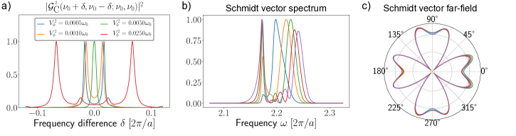
Figure 3: Two-particle scattering from a localized two-level system embedded in the inhomogeneous bath shown in Fig. 2a. We assume both the incident particles to be propagating along the xx axis (i.e. Ω1=Ω2=x^\Omega_{1}=\Omega_{2}=\hat{x}) for our simulations. a) The connected part of the two-excitation Green’s function as a function of the frequency difference between the two scattered particles assuming that the incident particles are at frequency ν0\nu_{0} resonant with the two-level system (ν0=ω0\nu_{0}=\omega_{0}). b) The frequency spectrum and c) the far field angular distribution of the first 5 Schmidt vectors of the output state corresponding to the connected part of the two-particle scattering matrix when both the input particles are Gaussian wave-packets in frequency (Eq. 48) with τ=220/ω0\tau=220/\omega_{0}.

Next, we consider two-particle scattering from the two-level system when it is embedded in the photonic crystal structure shown in Fig. 2a. Figure 3b shows the dependence of the connected part of the two-excitation Green’s function on the frequency difference of the output particles computed using Eq. 47. To study the spectral and spatial entanglement properties of the outgoing two-particles, we consider exciting the two-level system with a two-particle Fock state with both particles propagating along the x^\hat{{x}} axis but with a Gaussian spectrum:

|ψin(+e(νω0)2τ2/2a(x^,ν)dν)2|vac,g,\displaystyle\ket{\psi_{\text{in}}}\propto\bigg(\int_{\mathbb{R}^{+}}e^{-(\nu-\omega_{0})^{2}\tau^{2}/2}a^{\dagger}(\hat{x},\nu)d\nu\bigg)^{2}\ket{\text{vac},g}, (48)

where τ\tau governs the spectral bandwidth of the incident wave-packet. For large ω0τ1\omega_{0}\tau\gg 1, application of the connected part of the two-particle scattering matrix on this wave-packet yields the following two-particle wave-packet ψout,C(𝐱,ω)\psi_{\text{out,C}}(\vec{\mathbf{x}},\vec{\omega})

ψout,C(𝐱,ω)V04N0(ω0)2(𝐱d,x^,ω0)𝒢02(ω0)4π2×\displaystyle\psi_{\text{out,C}}(\vec{\mathbf{x}},\vec{\omega})\approx-\frac{V_{0}^{4}N_{0}(\omega_{0})\mathcal{E}^{2}(\mathbf{x}_{d},\hat{x},\omega_{0})\mathcal{G}_{0}^{2}(\omega_{0})}{4\pi^{2}}\times
(i=12𝒢0(ωi)G(𝐱i,𝐱d,ωi))e(ω1+ω22ω0)2τ2Γ(ω1+ω2).\displaystyle\qquad\bigg(\prod_{i=1}^{2}\mathcal{G}_{0}(\omega_{i})\text{G}(\mathbf{x}_{i},\mathbf{x}_{d};\omega_{i})\bigg)\frac{e^{-(\omega_{1}+\omega_{2}-2\omega_{0})^{2}\tau^{2}}}{\Gamma(\omega_{1}+\omega_{2})}. (49)

The Schmidt decomposition of ψout,C(𝐱,ω)\psi_{\text{out,C}}(\vec{\mathbf{x}},\vec{\omega}) can then express it as a superposition of two-particle fock states

ψout,C(𝐱,ω)=k=1λiψi(𝐱1,ω1)ψi(𝐱2,ω2),\displaystyle\psi_{\text{out,C}}(\vec{\mathbf{x}},\vec{\omega})=\sum_{k=1}^{\infty}\lambda_{i}\psi_{i}(\mathbf{x}_{1},\omega_{1})\psi_{i}(\mathbf{x}_{2},\omega_{2}), (50)

with λ1λ2λ3\lambda_{1}\geq\lambda_{2}\geq\lambda_{3}\dots. Figures 3b and c show the spectral and spatial dependence of the first five Schmidt components of ψout,C\psi_{\text{out,C}} for a two-level system strongly coupled to the photonic crystal bath. The frequency spectrum of each Schmidt vector (shown in Fig. 3b) is computed by integrating the magnitude square of the Schmidt vector over a sufficiently large circle surrounding the photonic crystal structure and the angular distribution of the far field (shown in Fig. 3c) is computed by integrating the magnitude square of the Schmidt vector with respect to frequency. The multi-Lorentzian nature of the spectrum of the emitted particles can be attributed to a strong hybridization between the two-level system and the electromagnetic modes of the photonic crystal cavity structure, while the far field pattern is almost completely determined by the field profile of the photonic crystal cavity mode.

IV Conclusion

In conclusion, we presented an approach to exactly analyze spatial and spectral properties of few-particle scattering from a localized system embedded in a an inhomogeneous bath. We develop exact solutions for the single and two-particle scattering matrices when the localized system is a two-level system. The formalism presented in this paper paves the way for computationally understanding the impact of structured media on quantum scattering from embedded localized systems. While the formalism in this paper assumes that the bosonic bath can be described by an inhomogeneous scalar wave equation, it can be extended to quantum optical systems where the bosonic bath (i.e. the photonic field) interacting with the localized system is described by a vector wave-equation.

V Acknowledgements

We thank David A. B. Miller and Geun Ho Ahn for providing feedback on the manuscript. R. T. acknowledges support from Kailath Graduate fellowship. This work is funded by the Air Force Office of Scientific Research under AFOSR MURI programme (award no. FA9550-17-1-0002).

References

  • (1) P. Lodahl, S. Mahmoodian, and S. Stobbe, “Interfacing single photons and single quantum dots with photonic nanostructures,” Reviews of Modern Physics, vol. 87, no. 2, p. 347, 2015. [Online]. Available: https://doi.org/10.1103/RevModPhys.87.347
  • (2) X. Ding, Y. He, Z.-C. Duan, N. Gregersen, M.-C. Chen, S. Unsleber, S. Maier, C. Schneider, M. Kamp, S. Höfling et al., “On-demand single photons with high extraction efficiency and near-unity indistinguishability from a resonantly driven quantum dot in a micropillar,” Physical Review Letters, vol. 116, no. 2, p. 020401, 2016. [Online]. Available: https://doi.org/10.1103/PhysRevLett.116.020401
  • (3) P. Michler, Ed., Quantum Dots for Quantum Information Technologies. Springer, 2017. [Online]. Available: https://doi.org/10.1007/978-3-319-56378-7
  • (4) P. Senellart, G. Solomon, and A. White, “High-performance semiconductor quantum-dot single-photon sources,” Nature Nanotechnology, vol. 12, no. 11, pp. nnano–2017, 2017. [Online]. Available: https://doi.org/10.1038/nnano.2017.218
  • (5) J. L. Zhang, S. Sun, M. J. Burek, C. Dory, Y.-K. Tzeng, K. A. Fischer, Y. Kelaita, K. G. Lagoudakis, M. Radulaski, Z.-X. Shen et al., “Strongly cavity-enhanced spontaneous emission from silicon-vacancy centers in diamond,” Nano letters, vol. 18, no. 2, pp. 1360–1365, 2018. [Online]. Available: https://doi.org/10.1021/acs.nanolett.7b05075
  • (6) P. Kok, W. J. Munro, K. Nemoto, T. C. Ralph, J. P. Dowling, and G. J. Milburn, “Linear optical quantum computing with photonic qubits,” Reviews of Modern Physics, vol. 79, no. 1, p. 135, 2007. [Online]. Available: https://doi.org/10.1103/RevModPhys.79.135
  • (7) J. L. O’brien, A. Furusawa, and J. Vučković, “Photonic quantum technologies,” Nature Photonics, vol. 3, no. 12, p. 687, 2009. [Online]. Available: https://doi.org/10.1038/nphoton.2009.229
  • (8) D. Roy, C. M. Wilson, and O. Firstenberg, “Colloquium: Strongly interacting photons in one-dimensional continuum,” Reviews of Modern Physics, vol. 89, no. 2, p. 021001, 2017. [Online]. Available: https://doi.org/10.1103/RevModPhys.89.021001
  • (9) A. Reiserer and G. Rempe, “Cavity-based quantum networks with single atoms and optical photons,” Reviews of Modern Physics, vol. 87, no. 4, p. 1379, 2015. [Online]. Available: https://doi.org/10.1103/RevModPhys.87.1379
  • (10) L.-M. Duan and C. Monroe, “Colloquium: Quantum networks with trapped ions,” Reviews of Modern Physics, vol. 82, no. 2, p. 1209, 2010. [Online]. Available: https://doi.org/10.1103/RevModPhys.82.1209
  • (11) N. Sangouard, C. Simon, H. De Riedmatten, and N. Gisin, “Quantum repeaters based on atomic ensembles and linear optics,” Reviews of Modern Physics, vol. 83, no. 1, p. 33, 2011. [Online]. Available: https://doi.org/10.1103/RevModPhys.83.33
  • (12) K. Nemoto, M. Trupke, S. J. Devitt, A. M. Stephens, B. Scharfenberger, K. Buczak, T. Nöbauer, M. S. Everitt, J. Schmiedmayer, and W. J. Munro, “Photonic architecture for scalable quantum information processing in diamond,” Physical Review X, vol. 4, no. 3, p. 031022, 2014. [Online]. Available: https://doi.org/10.1103/PhysRevX.4.031022
  • (13) D. Englund, D. Fattal, E. Waks, G. Solomon, B. Zhang, T. Nakaoka, Y. Arakawa, Y. Yamamoto, and J. Vučković, “Controlling the spontaneous emission rate of single quantum dots in a two-dimensional photonic crystal,” Physical review letters, vol. 95, no. 1, p. 013904, 2005. [Online]. Available: https://doi.org/10.1103/PhysRevLett.95.013904
  • (14) R. S. Daveau, K. C. Balram, T. Pregnolato, J. Liu, E. H. Lee, J. D. Song, V. Verma, R. Mirin, S. W. Nam, L. Midolo et al., “Efficient fiber-coupled single-photon source based on quantum dots in a photonic-crystal waveguide,” Optica, vol. 4, no. 2, pp. 178–184, 2017. [Online]. Available: https://doi.org/10.1364/OPTICA.4.000178
  • (15) M. Pelton, C. Santori, J. Vucković, B. Zhang, G. S. Solomon, J. Plant, and Y. Yamamoto, “Efficient source of single photons: a single quantum dot in a micropost microcavity,” Physical review letters, vol. 89, no. 23, p. 233602, 2002. [Online]. Available: https://doi.org/10.1103/PhysRevLett.89.233602
  • (16) Y.-M. He, Y. He, Y.-J. Wei, D. Wu, M. Atatüre, C. Schneider, S. Höfling, M. Kamp, C.-Y. Lu, and J.-W. Pan, “On-demand semiconductor single-photon source with near-unity indistinguishability,” Nature Nanotechnology, vol. 8, no. 3, pp. 213–217, 2013. [Online]. Available: https://doi.org/10.1038/nnano.2012.262
  • (17) K. A. Fischer, L. Hanschke, J. Wierzbowski, T. Simmet, C. Dory, J. J. Finley, J. Vučković, and K. Müller, “Signatures of two-photon pulses from a quantum two-level system,” Nature Physics, vol. 13, no. 7, pp. 649–654, 2017. [Online]. Available: https://doi.org/10.1038/nphys4052
  • (18) L. Hanschke, K. A. Fischer, S. Appel, D. Lukin, J. Wierzbowski, S. Sun, R. Trivedi, J. Vučković, J. J. Finley, and K. Müller, “Quantum dot single-photon sources with ultra-low multi-photon probability,” npj Quantum Information, vol. 4, no. 1, pp. 1–6, 2018. [Online]. Available: https://doi.org/10.1038/s41534-018-0092-0
  • (19) M. Metcalfe, S. M. Carr, A. Muller, G. S. Solomon, and J. Lawall, “Resolved sideband emission of inas/gaas quantum dots strained by surface acoustic waves,” Physical review letters, vol. 105, no. 3, p. 037401, 2010. [Online]. Available: https://doi.org/10.1103/PhysRevLett.105.037401
  • (20) K. C. Miao, A. Bourassa, C. P. Anderson, S. J. Whiteley, A. L. Crook, S. L. Bayliss, G. Wolfowicz, G. Thiering, P. Udvarhelyi, V. Ivády et al., “Electrically driven optical interferometry with spins in silicon carbide,” Science Advances, vol. 5, no. 11, p. eaay0527, 2019. [Online]. Available: https://doi.org/10.1126/sciadv.aay0527
  • (21) D. M. Lukin, A. D. White, R. Trivedi, M. A. Guidry, N. Morioka, C. Babin, Ö. O. Soykal, J. Ul-Hassan, N. T. Son, T. Ohshima et al., “Spectrally reconfigurable quantum emitters enabled by optimized fast modulation,” npj Quantum Information, vol. 6, no. 1, pp. 1–9, 2020. [Online]. Available: https://doi.org/10.1038/s41534-020-00310-0
  • (22) H. Wang, Y.-M. He, T.-H. Chung, H. Hu, Y. Yu, S. Chen, X. Ding, M.-C. Chen, J. Qin, X. Yang et al., “Towards optimal single-photon sources from polarized microcavities,” Nature Photonics, vol. 13, no. 11, pp. 770–775, 2019. [Online]. Available: https://doi.org/10.1038/s41566-019-0494-3
  • (23) X. Li, J. Chen, P. Voss, J. Sharping, and P. Kumar, “All-fiber photon-pair source for quantum communications: Improved generation of correlated photons,” Optics express, vol. 12, no. 16, pp. 3737–3744, 2004. [Online]. Available: https://doi.org/10.1364/OPEX.12.003737
  • (24) G. Harder, V. Ansari, B. Brecht, T. Dirmeier, C. Marquardt, and C. Silberhorn, “An optimized photon pair source for quantum circuits,” Optics express, vol. 21, no. 12, pp. 13 975–13 985, 2013. [Online]. Available: https://doi.org/10.1364/OE.21.013975
  • (25) H. Pichler and P. Zoller, “Photonic circuits with time delays and quantum feedback,” Physical review letters, vol. 116, no. 9, p. 093601, 2016. [Online]. Available: https://doi.org/10.1103/PhysRevLett.116.093601
  • (26) S. Xu and S. Fan, “Generate tensor network state by sequential single-photon scattering in waveguide qed systems,” APL Photonics, vol. 3, no. 11, p. 116102, 2018. [Online]. Available: https://doi.org/10.1063/1.5044248
  • (27) H. Carmichael, An open systems approach to quantum optics: lectures presented at the Université Libre de Bruxelles, October 28 to November 4, 1991. Springer Science & Business Media, 2009, vol. 18. [Online]. Available: https://doi.org/10.1007/978-3-540-47620-7
  • (28) C. Gardiner and P. Zoller, Quantum noise: a handbook of Markovian and non-Markovian quantum stochastic methods with applications to quantum optics. Springer Science & Business Media, 2004, vol. 56. [Online]. Available: https://doi.org/10.1007/9783540223016
  • (29) A. Asenjo-Garcia, J. Hood, D. Chang, and H. Kimble, “Atom-light interactions in quasi-one-dimensional nanostructures: A green’s-function perspective,” Physical Review A, vol. 95, no. 3, p. 033818, 2017. [Online]. Available: https://doi.org/10.1103/PhysRevA.95.033818
  • (30) H. T. Dung, L. Knöll, and D.-G. Welsch, “Resonant dipole-dipole interaction in the presence of dispersing and absorbing surroundings,” Physical Review A, vol. 66, no. 6, p. 063810, 2002. [Online]. Available: https://doi.org/10.1103/PhysRevA.66.063810
  • (31) A. H. Kiilerich and K. Mølmer, “Input-output theory with quantum pulses,” Physical review letters, vol. 123, no. 12, p. 123604, 2019. [Online]. Available: https://doi.org/10.1103/PhysRevLett.123.123604
  • (32) J. R. Taylor, Scattering theory: the quantum theory of nonrelativistic collisions. Courier Corporation, 2006.
  • (33) S. Fan, Ş. E. Kocabaş, and J.-T. Shen, “Input-output formalism for few-photon transport in one-dimensional nanophotonic waveguides coupled to a qubit,” Physical Review A, vol. 82, no. 6, p. 063821, 2010. [Online]. Available: https://doi.org/10.1103/PhysRevA.82.063821
  • (34) S. Xu, E. Rephaeli, and S. Fan, “Analytic properties of two-photon scattering matrix in integrated quantum systems determined by the cluster decomposition principle,” Physical review letters, vol. 111, no. 22, p. 223602, 2013. [Online]. Available: https://doi.org/10.1103/PhysRevLett.111.223602
  • (35) S. Xu and S. Fan, “Input-output formalism for few-photon transport: A systematic treatment beyond two photons,” Physical Review A, vol. 91, no. 4, p. 043845, 2015. [Online]. Available: https://doi.org/10.1103/PhysRevA.91.043845
  • (36) R. Trivedi, K. Fischer, S. Xu, S. Fan, and J. Vuckovic, “Few-photon scattering and emission from low-dimensional quantum systems,” Physical Review B, vol. 98, no. 14, p. 144112, 2018. [Online]. Available: https://doi.org/10.1103/PhysRevB.98.144112
  • (37) R. Trivedi, D. Malz, S. Sun, S. Fan, and J. Vučković, “Optimal two-photon excitation of bound states in non-markovian waveguide qed,” Physical Review A, vol. 104, no. 1, p. 013705, 2021.
  • (38) K. A. Fischer, R. Trivedi, V. Ramasesh, I. Siddiqi, and J. Vučković, “Scattering into one-dimensional waveguides from a coherently-driven quantum-optical system,” Quantum, vol. 2, p. 69, 2018. [Online]. Available: https://doi.org/10.22331/q-2018-05-28-69
  • (39) T. Shi, D. E. Chang, and J. I. Cirac, “Multiphoton-scattering theory and generalized master equations,” Physical Review A, vol. 92, no. 5, p. 053834, 2015. [Online]. Available: https://doi.org/10.1103/PhysRevA.92.053834
  • (40) T. Caneva, M. T. Manzoni, T. Shi, J. S. Douglas, J. I. Cirac, and D. E. Chang, “Quantum dynamics of propagating photons with strong interactions: a generalized input–output formalism,” New Journal of Physics, vol. 17, no. 11, p. 113001, 2015. [Online]. Available: http://dx.doi.org/10.1088/1367-2630/17/11/113001
  • (41) S. Haroche and D. Kleppner, “Cavity quantum electrodynamics,” Phys. Today, vol. 42, no. 1, pp. 24–30, 1989. [Online]. Available: http://dx.doi.org/10.1063/1.881201
  • (42) R. Trivedi, M. Radulaski, K. A. Fischer, S. Fan, and J. Vučković, “Photon blockade in weakly driven cavity quantum electrodynamics systems with many emitters,” Physical review letters, vol. 122, no. 24, p. 243602, 2019. [Online]. Available: https://doi.org/10.1103/PhysRevLett.122.243602
  • (43) T. Shi, S. Fan et al., “Two-photon transport through a waveguide coupling to a whispering-gallery resonator containing an atom and photon-blockade effect,” Physical Review A, vol. 87, no. 6, p. 063818, 2013. [Online]. Available: https://doi.org/10.1103/PhysRevA.87.063818
  • (44) J. Liu, M. Zhou, and Z. Yu, “Quantum scattering theory of a single-photon fock state in three-dimensional spaces,” Optics letters, vol. 41, no. 18, pp. 4166–4169, 2016. [Online]. Available: https://doi.org/10.1364/OL.41.004166
  • (45) M. Orenstein, S. Fan et al., “Two-level quantum system as a macroscopic scatterer for ultraconfined two-dimensional photonic modes,” Physical Review A, vol. 102, no. 1, p. 013717, 2020. [Online]. Available: https://doi.org/10.1103/PhysRevA.102.013717
  • (46) E. K. Miller, “A selective survey of computational electromagnetics,” IEEE Transactions on Antennas and Propagation, vol. 36, no. 9, pp. 1281–1305, 1988. [Online]. Available: https://doi.org/10.1109/8.8607
  • (47) S. Molesky, Z. Lin, A. Y. Piggott, W. Jin, J. Vucković, and A. W. Rodriguez, “Inverse design in nanophotonics,” Nature Photonics, vol. 12, no. 11, pp. 659–670, 2018. [Online]. Available: https://doi.org/10.1038/s41566-018-0246-9
  • (48) H. T. Dung, L. Knöll, and D.-G. Welsch, “Three-dimensional quantization of the electromagnetic field in dispersive and absorbing inhomogeneous dielectrics,” Physical Review A, vol. 57, no. 5, p. 3931, 1998. [Online]. Available: https://doi.org/10.1103/PhysRevA.57.3931
  • (49) T. Gruner and D.-G. Welsch, “Green-function approach to the radiation-field quantization for homogeneous and inhomogeneous kramers-kronig dielectrics,” Physical Review A, vol. 53, no. 3, p. 1818, 1996. [Online]. Available: https://doi.org/10.1103/PhysRevA.53.1818
  • (50) S. Weinberg, The quantum theory of fields. Cambridge university press, 1995, vol. 2. [Online]. Available: https://doi.org/10.1017/CBO9781139644167
  • (51) H.-P. Breuer and F. Petruccione, The theory of open quantum systems. Oxford University Press on Demand, 2002. [Online]. Available: https://doi.org/10.1093/acprof:oso/9780199213900.001.0001
  • (52) Y. Wang and I. Khoo, “On the wigner-weisskopf approximation in quantum optics,” Optics Communications, vol. 11, no. 4, pp. 323–326, 1974. [Online]. Available: https://doi.org/10.1016/0030-4018(74)90227-2

Appendix A Second quantization with noise operators

We begin by outlining some useful properties of the scalar Green’s function corresponding to the inhomogeneous wave-equation, followed by showing that the noise-operator based quantum theory presented in the main text satisfies the canonical commutation relations stemming from Dirac’s quantization.

A.1 Properties of the scalar inhomogeneous Green’s function

Throughout this section, Gα(𝐱,𝐱,ω)\text{G}_{\alpha}(\mathbf{x},\mathbf{x}^{\prime};\omega) will refer to the scalar’s green’s function which satisfies

[𝐱2+ω2εα(𝐱,ω)]Gα(𝐱,𝐱,ω)=δ3(𝐱𝐱),\displaystyle\big[\nabla^{2}_{\mathbf{x}}+\omega^{2}\varepsilon_{\alpha}(\mathbf{x},\omega)\big]\text{G}_{\alpha}(\mathbf{x},\mathbf{x}^{\prime};\omega)=\delta^{3}(\mathbf{x}-\mathbf{x}^{\prime}), (51)

where εα(ω)=ε(𝐱)+iα(ω)\varepsilon_{\alpha}(\omega)=\varepsilon(\mathbf{x})+i\alpha(\omega). Here ε(𝐱)\varepsilon(\mathbf{x}) is the inhomogeneous permittivity distribution corresponding to the inhomogenuous media and α(ω)\alpha(\omega) governs the loss in the media. We point out that while physically ω>0\omega>0, it is convenient to consider the solution of Eq. 51 for ω<0\omega<0 as well. We assume that for ω>0,α(ω)=α(ω)\omega>0,\alpha(-\omega)=-\alpha(\omega) — this ensures that for ω<0,α(ω)<0\omega<0,\alpha(\omega)<0 and hence the outgoing solution to Eq. 51 for ω<0\omega<0 decays exponentially as |𝐱||\mathbf{x}|\to\infty. Furthermore, we also make a physically reasonable assumption of α(ω)0\alpha(\omega)\to 0 as |ω||\omega|\to\infty.

Property 1:

Gα(𝐱,𝐱,ω)=Gα(𝐱,𝐱,ω).\displaystyle\text{G}_{\alpha}(\mathbf{x},\mathbf{x}^{\prime};\omega)=\text{G}_{\alpha}^{*}(\mathbf{x},\mathbf{x}^{\prime};-\omega). (52)

Proof: This immediately follows by conjugating Eq. 51 and by noting that εα(𝐱,ω)=εα(𝐱,ω)\varepsilon_{\alpha}(\mathbf{x},-\omega)=\varepsilon_{\alpha}^{*}(\mathbf{x},\omega).


Property 2:

2iω2α3Gα(𝐱,𝐲,ω)Gα(𝐱,𝐲,ω)d3𝐲=Gα(𝐱,𝐱,ω)Gα(𝐱,𝐱,ω).\displaystyle 2i\omega^{2}\alpha\int_{\mathbb{R}^{3}}\text{G}_{\alpha}^{*}(\mathbf{x}^{\prime},\mathbf{y};\omega)\text{G}_{\alpha}(\mathbf{x},\mathbf{y};\omega)d^{3}\mathbf{y}=\text{G}_{\alpha}^{*}(\mathbf{x},\mathbf{x}^{\prime};\omega)-\text{G}_{\alpha}(\mathbf{x},\mathbf{x}^{\prime};\omega). (53)

Proof: We note that the scalar Green’s function is necessarily reciprocal i.e. Gα(𝐱,𝐲,ω)=Gα(𝐲,𝐱,ω)\text{G}_{\alpha}(\mathbf{x},\mathbf{y};\omega)=\text{G}_{\alpha}(\mathbf{y},\mathbf{x};\omega). Therefore, it follows from Eq. 51 that

[𝐲2+ω2εα(𝐲,ω)]Gα(𝐱,𝐲,ω)=δ3(𝐱𝐲).\displaystyle\big[\nabla^{2}_{\mathbf{y}}+\omega^{2}\varepsilon_{\alpha}(\mathbf{y};\omega)\big]\text{G}_{\alpha}(\mathbf{x},\mathbf{y};\omega)=\delta^{3}(\mathbf{x}-\mathbf{y}). (54)

Multiplying this equation with Gα(𝐱,𝐲,ω)\text{G}_{\alpha}^{*}(\mathbf{x}^{\prime},\mathbf{y};\omega) and integrating with respect to 𝐲\mathbf{y} we obtain

Gα(𝐱,𝐱;ω)=3𝐲Gα(𝐱,𝐲;ω)𝐲Gα(𝐱,𝐲;ω)d3𝐲+ω23εα(𝐲;ω)Gα(𝐱,𝐲;ω)Gα(𝐱,𝐲;ω)d3𝐲.\displaystyle\text{G}_{\alpha}^{*}(\mathbf{x},\mathbf{x}^{\prime};\omega)=-\int_{\mathbb{R}^{3}}\nabla_{\mathbf{y}}\text{G}_{\alpha}^{*}(\mathbf{x}^{\prime},\mathbf{y};\omega)\cdot\nabla_{\mathbf{y}}\text{G}_{\alpha}(\mathbf{x},\mathbf{y};\omega)d^{3}\mathbf{y}+\omega^{2}\int_{\mathbb{R}^{3}}\varepsilon_{\alpha}(\mathbf{y};\omega)\text{G}_{\alpha}^{*}(\mathbf{x}^{\prime},\mathbf{y};\omega)\text{G}_{\alpha}(\mathbf{x},\mathbf{y};\omega)d^{3}\mathbf{y}. (55)

Conjugating Eq. 55 followed by swapping 𝐱\mathbf{x} and 𝐱\mathbf{x}^{\prime}, we obtain

Gα(𝐱,𝐱;ω)=3𝐲Gα(𝐱,𝐲;ω)𝐲Gα(𝐱,𝐲;ω)d3𝐲+ω23εα(𝐲;ω)Gα(𝐱,𝐲;ω)Gα(𝐱,𝐲;ω)d3𝐲.\displaystyle\text{G}_{\alpha}(\mathbf{x},\mathbf{x}^{\prime};\omega)=-\int_{\mathbb{R}^{3}}\nabla_{\mathbf{y}}\text{G}_{\alpha}^{*}(\mathbf{x}^{\prime},\mathbf{y};\omega)\cdot\nabla_{\mathbf{y}}\text{G}_{\alpha}(\mathbf{x},\mathbf{y};\omega)d^{3}\mathbf{y}+\omega^{2}\int_{\mathbb{R}^{3}}\varepsilon_{\alpha}^{*}(\mathbf{y};\omega)\text{G}_{\alpha}^{*}(\mathbf{x}^{\prime},\mathbf{y};\omega)\text{G}_{\alpha}(\mathbf{x},\mathbf{y};\omega)d^{3}\mathbf{y}. (56)

Subtracting Eq. 56 from Eq. 55, we obtain Eq. 53.


Property 3: Assuming that εub\exists\ \varepsilon_{\text{ub}} such that ε(𝐱)<εUB𝐱\varepsilon(\mathbf{x})<\varepsilon_{\text{UB}}\ \forall\ \mathbf{x} and ε(𝐱)>0𝐱\varepsilon(\mathbf{x})>0\ \forall\ \mathbf{x},

ωGα(𝐱,𝐱,ω)𝑑ω=iπε(𝐱)δ3(𝐱𝐱).\displaystyle\int_{-\infty}^{\infty}\omega\text{G}_{\alpha}(\mathbf{x},\mathbf{x}^{\prime};\omega)\ d\omega=-\frac{i\pi}{\varepsilon(\mathbf{x})}\delta^{3}(\mathbf{x}-\mathbf{x}^{\prime}). (57)

Proof: Defining θ(𝐱)=εubε(𝐱)\theta(\mathbf{x})=\varepsilon_{\text{ub}}-\varepsilon(\mathbf{x}), Eq. 51 can be rewritten as

[𝐱2+ω2(εub+iα(ω))]Gα(𝐱,𝐱,ω)=ω2θ(𝐱)Gα(𝐱,𝐱,ω)+δ3(𝐱𝐱).\displaystyle\big[\nabla^{2}_{\mathbf{x}}+\omega^{2}(\varepsilon_{\text{ub}}+i\alpha(\omega))\big]\text{G}_{\alpha}(\mathbf{x},\mathbf{x}^{\prime};\omega)=\omega^{2}\theta(\mathbf{x})\text{G}_{\alpha}(\mathbf{x},\mathbf{x}^{\prime};\omega)+\delta^{3}(\mathbf{x}-\mathbf{x}^{\prime}). (58)

A Dyson series for Gα(𝐱,𝐱,ω)\text{G}_{\alpha}(\mathbf{x},\mathbf{x}^{\prime};\omega) can be deduced from Eq. 58 to obtain

Gα(𝐱,𝐱,ω)=Gαub(𝐱,𝐱,ω)+n=1ω2k𝐲1,𝐲2𝐲k3[k=0nGαub(𝐲k,𝐲k+1,ω)]𝐲0=𝐱𝐲n+1=𝐱[k=1nθ(𝐲k)d3𝐲k],\displaystyle\text{G}_{\alpha}(\mathbf{x},\mathbf{x}^{\prime};\omega)=\text{G}_{\alpha}^{\text{ub}}(\mathbf{x},\mathbf{x}^{\prime};\omega)+\sum_{n=1}^{\infty}\omega^{2k}\int_{\mathbf{y}_{1},\mathbf{y}_{2}\dots\mathbf{y}_{k}\in\mathbb{R}^{3}}\bigg[\prod_{k=0}^{n}\text{G}_{\alpha}^{\text{ub}}(\mathbf{y}_{k},\mathbf{y}_{k+1};\omega)\bigg]_{\begin{subarray}{c}\mathbf{y}_{0}=\mathbf{x}\\ \mathbf{y}_{n+1}=\mathbf{x}^{\prime}\end{subarray}}\bigg[\prod_{k=1}^{n}\theta(\mathbf{y}_{k})d^{3}\mathbf{y}_{k}\bigg], (59)

where Gαub(𝐱,𝐱,ω)\text{G}_{\alpha}^{\text{ub}}(\mathbf{x},\mathbf{x}^{\prime};\omega) satisfies

[𝐱2+ω2(εub+iα(ω))]Gαub(𝐱,𝐱,ω)=δ3(𝐱𝐱).\displaystyle\big[\nabla_{\mathbf{x}}^{2}+\omega^{2}(\varepsilon_{\text{ub}}+i\alpha(\omega))\big]\text{G}_{\alpha}^{\text{ub}}(\mathbf{x},\mathbf{x}^{\prime};\omega)=\delta^{3}(\mathbf{x}-\mathbf{x}^{\prime}). (60)

It can easily be seen from Eq. 60 that

Gαub(𝐱,𝐱,ω)=3ei𝐤(𝐱𝐱)ω2εub|𝐤|2+iω2α(ω)d3𝐤(2π)3.\displaystyle\text{G}_{\alpha}^{\text{ub}}(\mathbf{x},\mathbf{x}^{\prime};\omega)=\int_{\mathbb{R}^{3}}\frac{e^{i\mathbf{k}\cdot(\mathbf{x}-\mathbf{x}^{\prime})}}{\omega^{2}\varepsilon_{\text{ub}}-|\mathbf{k}|^{2}+i\omega^{2}\alpha(\omega)}\frac{d^{3}\mathbf{k}}{(2\pi)^{3}}. (61)

We next evaluate the integral in Eq. 57 using the expansion for Gα(𝐱,𝐱,ω)\text{G}_{\alpha}(\mathbf{x},\mathbf{x}^{\prime};\omega) in Eq. 59. Consider the following integral

ω2k+1\displaystyle\int_{-\infty}^{\infty}\omega^{2k+1} [k=0nGαub(𝐲k,𝐲k+1,ω)]𝑑ω=ω𝐤0,𝐤1𝐤n3ω2k+1[k=0nei𝐤k(𝐲k𝐲k+1)ω2εub|𝐤k|2+iω2α(ω)d3𝐤k(2π)3]𝑑ω.\displaystyle\bigg[\prod_{k=0}^{n}\text{G}_{\alpha}^{\text{ub}}(\mathbf{y}_{k},\mathbf{y}_{k+1};\omega)\bigg]d\omega=\int_{\omega\in\mathbb{R}}\int_{\mathbf{k}_{0},\mathbf{k}_{1}\dots\mathbf{k}_{n}\in\mathbb{R}^{3}}\omega^{2k+1}\bigg[\prod_{k=0}^{n}\frac{e^{i\mathbf{k}_{k}\cdot(\mathbf{y}_{k}-\mathbf{y}_{k+1})}}{\omega^{2}\varepsilon_{\text{ub}}-|\mathbf{k}_{k}|^{2}+i\omega^{2}\alpha(\omega)}\frac{d^{3}\mathbf{k}_{k}}{(2\pi)^{3}}\bigg]d\omega. (62)

Noting that the integrand is analytic as a function of ω\omega in the upper complex half-plane, it follows that the integral with respect to ω\omega can be evaluated along ω=Reiθ\omega=Re^{i\theta}, with RR\to\infty with θ\theta going from π\pi to 00. This immediately yields

ω2k+1[k=0nGαub(𝐲k,𝐲k+1;ω)]dω=iπεubk=0nδ3(𝐲k𝐲k+1).\displaystyle\int_{-\infty}^{\infty}\omega^{2k+1}\bigg[\prod_{k=0}^{n}\text{G}_{\alpha}^{\text{ub}}(\mathbf{y}_{k},\mathbf{y}_{k+1};\omega)\bigg]d\omega=-\frac{i\pi}{\varepsilon_{\text{ub}}}\prod_{k=0}^{n}\delta^{3}(\mathbf{y}_{k}-\mathbf{y}_{k+1}). (63)

It thus follows from Eq. 59 that

ωGαub(𝐱,𝐱;ω)=iπδ3(𝐱𝐱)k=0θk(𝐱)εubk+1=iπε(𝐱)δ3(𝐱𝐱).\displaystyle\int_{-\infty}^{\infty}\omega\text{G}_{\alpha}^{\text{ub}}(\mathbf{x},\mathbf{x}^{\prime};\omega)=-i\pi\delta^{3}(\mathbf{x}-\mathbf{x}^{\prime})\sum_{k=0}^{\infty}\frac{\theta^{k}(\mathbf{x})}{\varepsilon_{\text{ub}}^{k+1}}=-\frac{i\pi}{\varepsilon(\mathbf{x})}\delta^{3}(\mathbf{x}-\mathbf{x}^{\prime}). (64)

A.2 Verifying canonical commutation relations between ψ(𝐱)\psi(\mathbf{x}) and π(𝐱)\pi(\mathbf{x})

We begin by deriving the commutator [ψ(𝐱,ω),ψ(𝐱,ω)][\psi(\mathbf{x},\omega),\psi^{\dagger}(\mathbf{x}^{\prime},\omega^{\prime})]. Using Eq. II.2.1 and the commutator for the noise operator ψ(𝐱,ω)\psi(\mathbf{x},\omega), we obtain

[ψ(𝐱,ω),ψ(𝐱,ω)]=1πω2α(ω)δ(ωω)3Gα(𝐱,𝐲,ω)Gα(𝐱,𝐲,ω)d3𝐲.\displaystyle[\psi(\mathbf{x},\omega),\psi^{\dagger}(\mathbf{x}^{\prime};\omega^{\prime})]=\frac{1}{\pi}\omega^{2}\alpha(\omega)\delta(\omega-\omega^{\prime})\int_{\mathbb{R}^{3}}\text{G}_{\alpha}^{*}(\mathbf{x}^{\prime},\mathbf{y};\omega)\text{G}_{\alpha}(\mathbf{x},\mathbf{y};\omega)d^{3}\mathbf{y}. (65)

Using Eq. 53, we obtain

[ψ(𝐱,ω),ψ(𝐱,ω)]\displaystyle[\psi(\mathbf{x},\omega),\psi^{\dagger}(\mathbf{x}^{\prime};\omega^{\prime})] =δ(ωω)2πi[Gα(𝐱,𝐱,ω)Gα(𝐱,𝐱,ω)],\displaystyle=\frac{\delta(\omega-\omega^{\prime})}{2\pi i}\big[\text{G}_{\alpha}^{*}(\mathbf{x},\mathbf{x}^{\prime};\omega)-\text{G}_{\alpha}(\mathbf{x},\mathbf{x}^{\prime};\omega)\big],
=δ(ωω)2πIm[Gα(𝐱,𝐱,ω)].\displaystyle=-\frac{\delta(\omega-\omega^{\prime})}{2\pi}\text{Im}\big[\text{G}_{\alpha}(\mathbf{x},\mathbf{x}^{\prime};\omega)\big]. (66)

Consider now the commutator [ψ(𝐱),π(𝐱)][\psi(\mathbf{x}),\pi(\mathbf{x}^{\prime})]: Using Eqs. 9a and A.2, we obtain

[ψ(𝐱),π(𝐱)]=ε(𝐱)πω+ω[Gα(𝐱,𝐱,ω)Gα(𝐱,𝐱,ω)]𝑑ω.\displaystyle[\psi(\mathbf{x}),\pi(\mathbf{x}^{\prime})]=\frac{\varepsilon(\mathbf{x}^{\prime})}{\pi}\int_{\omega\in\mathbb{R}^{+}}\omega\big[\text{G}_{\alpha}^{*}(\mathbf{x},\mathbf{x}^{\prime};\omega)-\text{G}_{\alpha}(\mathbf{x},\mathbf{x}^{\prime};\omega)\big]d\omega. (67)

Using Eqs. 52 and 57, it immediately follows that [ψ(𝐱),π(𝐱)]=iδ3(𝐱𝐱)[\psi(\mathbf{x}),\pi(\mathbf{x}^{\prime})]=i\delta^{3}(\mathbf{x}-\mathbf{x}^{\prime}) — the noise operator based quantization thus reproduces the canonical commutation relations for inhomogeneous bosonic baths.

Appendix B Evaluating aα(𝐱,Ω,ω)a_{\alpha}(\mathbf{x},\Omega,\omega) as α(ω)0\alpha(\omega)\to 0

In this appendix, we detail the evaluation of the limα(ω)0aα(𝐱,Ω,ω)\lim_{\alpha(\omega)\to 0}a_{\alpha}(\mathbf{x},\Omega;\omega), where aα(𝐱,Ω,ω)a_{\alpha}(\mathbf{x},\Omega;\omega) is defined in Eq. II.2.2. In particular, we show that in the limit of α(ω)0\alpha(\omega)\to 0, aα(𝐱,Ω,ω)a_{\alpha}(\mathbf{x},\Omega;\omega) becomes independent of 𝐱\mathbf{x}. Since aα(𝐱,Ω,ω)a_{\alpha}(\mathbf{x},\Omega;\omega) are, by construction, bosonic annihilation operators, in order to show that limα(ω)0aα(𝐱,Ω,ω)\lim_{\alpha(\omega)\to 0}a_{\alpha}(\mathbf{x},\Omega;\omega) is independent of 𝐱\mathbf{x}, it is sufficient to show that limα(ω)0[aα(𝐱,Ω,ω),aα(𝐱,Ω,ω)]\lim_{\alpha(\omega)\to 0}[a_{\alpha}(\mathbf{x},\Omega;\omega),a_{\alpha}^{\dagger}(\mathbf{x}^{\prime},\Omega^{\prime};\omega^{\prime})] is independent of 𝐱\mathbf{x} and 𝐱\mathbf{x}^{\prime}. Using Eq. II.2.2 and [ϕα(𝐱,ω),ϕα(𝐱,ω)]=δ3(𝐱𝐱)δ(ωω)[\phi_{\alpha}(\mathbf{x};\omega),\phi^{\dagger}_{\alpha}(\mathbf{x}^{\prime};\omega^{\prime})]=\delta^{3}(\mathbf{x}-\mathbf{x}^{\prime})\delta(\omega-\omega^{\prime}), we can explicitly evaluate this commutator to obtain

[aα(𝐱,\displaystyle[a_{\alpha}(\mathbf{x}, OPENOPENΩ;ω),aα(𝐱,Ω,ω)]=\displaystyle\Omega;\omega),a_{\alpha}^{\dagger}(\mathbf{x}^{\prime},\Omega^{\prime};\omega^{\prime})]=
α(ω)ω4π4ε0δ(ωω)𝐲3k,k+k2k2ei(kΩkΩ)𝐲ei(kk0(ω))Ω𝐱ei(kk0(ω))Ω𝐱(ω2ε0k2+iω2α(ω))(ω2ε0k2iω2α(ω))𝑑kdkd3𝐲.\displaystyle\frac{\alpha(\omega)\omega}{4\pi^{4}\sqrt{\varepsilon_{0}}}\delta(\omega-\omega^{\prime})\int_{\begin{subarray}{c}\mathbf{y}\in\mathbb{R}^{3}\\ k,k^{\prime}\in\mathbb{R}^{+}\end{subarray}}\frac{k^{2}k^{\prime 2}e^{i(k\Omega-k^{\prime}\Omega^{\prime})\cdot\mathbf{y}}e^{i(k-k_{0}(\omega))\Omega\cdot\mathbf{x}}e^{-i(k^{\prime}-k_{0}(\omega))\Omega^{\prime}\cdot\mathbf{x}^{\prime}}}{(\omega^{2}\varepsilon_{0}-k^{2}+i\omega^{2}\alpha(\omega))(\omega^{2}\varepsilon_{0}-k^{\prime 2}-i\omega^{2}\alpha(\omega))}dkdk^{\prime}d^{3}\mathbf{y}. (68)

Noting that

3ei(kΩkΩ)𝐲d3𝐲=8π3δ(kk)δ2(ΩΩ)k2,\displaystyle\int_{\mathbb{R}^{3}}e^{i(k\Omega-k^{\prime}\Omega^{\prime})\cdot\mathbf{y}}d^{3}\mathbf{y}=\frac{8\pi^{3}\delta(k-k^{\prime})\delta^{2}(\Omega-\Omega^{\prime})}{k^{2}}, (69)

we obtain

[aα(𝐱,Ω,ω),aα(𝐱,Ω,ω)]=2α(ω)ωπε0δ(ωω)δ2(ΩΩ)+k2ei(kk0(ω))Ω(𝐱𝐱)(ω2ε0k2)2+ω4σ2(ω)𝑑k.\displaystyle[a_{\alpha}(\mathbf{x},\Omega;\omega),a_{\alpha}^{\dagger}(\mathbf{x}^{\prime},\Omega^{\prime};\omega^{\prime})]=\frac{2\alpha(\omega)\omega}{\pi\sqrt{\varepsilon_{0}}}\delta(\omega-\omega^{\prime})\delta^{2}(\Omega-\Omega^{\prime})\int_{\mathbb{R}^{+}}\frac{k^{2}e^{i(k-k_{0}(\omega))\Omega\cdot(\mathbf{x}-\mathbf{x}^{\prime})}}{(\omega^{2}\varepsilon_{0}-k^{2})^{2}+\omega^{4}\sigma^{2}(\omega)}dk. (70)

We note that in the limit of α(ω)0\alpha(\omega)\to 0, the integral in the above equation can be approximated as follows

+k2ei(kk0(ω))Ω(𝐱𝐱)(ω2ε0k2)2+ω2σ4(ω)𝑑k14+1(kωε0)2+ω2σ2(ω)/4ε0πε02ωα(ω).\displaystyle\int_{\mathbb{R}^{+}}\frac{k^{2}e^{i(k-k_{0}(\omega))\Omega\cdot(\mathbf{x}-\mathbf{x}^{\prime})}}{(\omega^{2}\varepsilon_{0}-k^{2})^{2}+\omega^{2}\sigma^{4}(\omega)}dk\approx\frac{1}{4}\int_{\mathbb{R}^{+}}\frac{1}{(k-\omega\sqrt{\varepsilon_{0}})^{2}+\omega^{2}\sigma^{2}(\omega)/4\varepsilon_{0}}\approx\frac{\pi\sqrt{\varepsilon_{0}}}{2\omega\alpha(\omega)}. (71)

Consequently, we obtain

limα(ω)0[aα(𝐱,Ω,ω),aα(𝐱,Ω,ω)]=δ(ωω)δ2(ΩΩ).\displaystyle\lim_{\alpha(\omega)\to 0}[a_{\alpha}(\mathbf{x},\Omega;\omega),a_{\alpha}^{\dagger}(\mathbf{x}^{\prime},\Omega^{\prime};\omega^{\prime})]=\delta(\omega-\omega^{\prime})\delta^{2}(\Omega-\Omega^{\prime}). (72)

Thus, we conclude that the operators aσ(𝐱,Ω,ω)a_{\sigma}(\mathbf{x},\Omega;\omega) are independent of 𝐱\mathbf{x} in the limit of α(ω)0\alpha(\omega)\to 0. Defining a(Ω,ω)a(\Omega;\omega) via a(Ω,ω)=limα(ω)0aα(𝐱,Ω,ω)a(\Omega;\omega)=\lim_{\alpha(\omega)\to 0}a_{\alpha}(\mathbf{x},\Omega;\omega), we thus obtain the following commutator

[a(Ω,ω),a(Ω,ω)]=δ(ωω)δ2(ΩΩ).\displaystyle[a(\Omega;\omega),a^{\dagger}(\Omega^{\prime};\omega^{\prime})]=\delta(\omega-\omega^{\prime})\delta^{2}(\Omega-\Omega^{\prime}). (73)

Appendix C Relating scattering matrix to the localized system’s Green’s functions

Our starting point is the Heisenberg picture representation of the NN-particle scattering matrix element in Eq. III. We first substitute for ψ(𝐱,ω,tf)\psi(\mathbf{x},\omega;t_{f}) from Eq. 29 to obtain

ein=1Nωntfvac,g|𝒯[i=1Nψ(𝐱i,ωi,tf)i=1Na(Ωi,νi,ti)]|vac,g\displaystyle e^{i\sum_{n=1}^{N}\omega_{n}t_{f}}\bra{\text{vac},g}\mathcal{T}\bigg[\prod_{i=1}^{N}\psi(\mathbf{x}_{i},\omega_{i};t_{f})\prod_{i=1}^{N}a^{\dagger}(\Omega_{i},\nu_{i};t_{i})\bigg]\ket{\text{vac},g}
=vac,g|k=0NkN𝒯[(n¯kNV0πIm[G(𝐱n,𝐱d;ωn)]titfσ(τ)eiωnτdτ)(nkNψ(𝐱n,ωn;ti)eiωnti)×\displaystyle=\bra{\text{vac},g}\sum_{k=0}^{N}\sum_{\mathcal{B}_{k}^{N}}\mathcal{T}\bigg[\bigg(\prod_{n\in\bar{\mathcal{B}}_{k}^{N}}\frac{V_{0}}{\pi}\text{Im}\big[\text{G}(\mathbf{x}_{n},\mathbf{x}_{d};\omega_{n})\big]\int_{t_{i}}^{t_{f}}\sigma(\tau)e^{i\omega_{n}\tau}d\tau\bigg)\bigg(\prod_{n\in\mathcal{B}_{k}^{N}}\psi(\mathbf{x}_{n},\omega_{n};t_{i})e^{i\omega_{n}t_{i}}\bigg)\times
(n=1Na(Ωn,νn;ti))]|vac,g,\displaystyle\bigg(\prod_{n=1}^{N}a^{\dagger}(\Omega_{n},\nu_{n};t_{i})\bigg)\bigg]\ket{\text{vac},g}, (74)

where kN\mathcal{B}_{k}^{N} is an unordered kk-element subset of {1,2,N}\{1,2,\dots N\}, and ¯kN\bar{\mathcal{B}}_{k}^{N} is its complement. Using the commutator [ψ(𝐱,ω),a(Ω,ν)]=N0(ν)(𝐱,Ω,ν)δ(ων)[\psi(\mathbf{x},\omega),a^{\dagger}(\Omega,\nu)]=N_{0}(\nu)\mathcal{E}(\mathbf{x},\Omega,\nu)\delta(\omega-\nu) and the relation ψ(𝐱,ω,ti)|vac,g=0\psi(\mathbf{x},\omega;t_{i})\ket{\text{vac},g}=0, we obtain

(nkNψ(𝐱n,ωn,ti))n=1Na(Ωn,νn,ti)|vac,g=\displaystyle\bigg(\prod_{n\in\mathcal{B}_{k}^{N}}\psi(\mathbf{x}_{n},\omega_{n};t_{i})\bigg)\prod_{n=1}^{N}a^{\dagger}(\Omega_{n},\nu_{n};t_{i})\ket{\text{vac},g}=
𝒟kN,𝒫k(n=1Nka(Ω𝒟¯kN(n),ν𝒟¯kN(n),ti))(n=1kN0(ν𝒟kN(n))(𝐱𝒫kkN(n),Ω𝒟kN(n),ν𝒟kN(n))δ(ω𝒫kkN(n)ν𝒟kN(n))),\displaystyle\sum_{\mathcal{D}_{k}^{N},\mathcal{P}_{k}}\bigg(\prod_{n=1}^{N-k}a^{\dagger}(\Omega_{\bar{\mathcal{D}}_{k}^{N}(n)},\nu_{\bar{\mathcal{D}}_{k}^{N}(n)};t_{i})\bigg)\bigg(\prod_{n=1}^{k}N_{0}\big(\nu_{\mathcal{D}_{k}^{N}(n)}\big)\mathcal{E}\big(\mathbf{x}_{\mathcal{P}_{k}\mathcal{B}_{k}^{N}(n)},\Omega_{\mathcal{D}_{k}^{N}(n)};\nu_{\mathcal{D}_{k}^{N}(n)}\big)\delta\big(\omega_{\mathcal{P}_{k}\mathcal{B}_{k}^{N}(n)}-\nu_{\mathcal{D}_{k}^{N}(n)}\big)\bigg), (75)

where 𝒟kN\mathcal{D}_{k}^{N} is another unordered kk-element subset of {1,2N}\{1,2\dots N\} with 𝒟¯kN\bar{\mathcal{D}}^{N}_{k} being its complement, 𝒫k\mathcal{P}_{k} is a kk- element permutation and 𝒫k𝒟kN\mathcal{P}_{k}\mathcal{D}_{k}^{N} is a permutation of the kk-element subset 𝒟kN\mathcal{D}_{k}^{N}. Next, we substitute Eq. C into Eq. C and use Eq. III to substitute for a(Ω,ν,ti)a^{\dagger}(\Omega,\nu;t_{i}) in terms of a(Ω,ν,tf)a^{\dagger}(\Omega,\nu;t_{f}). We note that due to the time-ordering operator, a^(Ω,ν,tf)\hat{a}^{\dagger}(\Omega,\nu;t_{f}) annihilate vac,g|\bra{\text{vac},g}. With this simplification, we obtain Eq. III in the main text.

Appendix D Computing single and two-excitation Green’s functions

In this section, we outline the numerical procedures used for computing the single and two-excitation Green’s function that are needed for calculating the single and two-excitation scattering matrices.

D.1 Single-excitation Green’s function

The single-excitation Green’s function in time-domain, 𝒢(t,t)\mathcal{G}(t;t^{\prime}), is given by

𝒢(t,s)=g,vac|𝒯[σ(t)σ(s)]|g,vac,\displaystyle\mathcal{G}(t,s)=\bra{g,\text{vac}}\mathcal{T}\big[\sigma(t)\sigma^{\dagger}(s)\big]\ket{g,\text{vac}}, (76)

where σ(t)\sigma(t) and σ(t)\sigma^{\dagger}(t) are the Heisenberg picture operators corresponding to the two-level system’s lowering and raising operators. Since σ(t)|g,vac=0\sigma(t)\ket{g,\text{vac}}=0 and g,vac|σ(t)=0\bra{g,\text{vac}}\sigma^{\dagger}(t)=0 for all tt, we obtain an alternative representation of the single-excitation Green’s function

𝒢(t,s)=e,vac|eiH(ts)|e,vacΘ(tt),\displaystyle\mathcal{G}(t,s)=\bra{e,\text{vac}}e^{-iH(t-s)}\ket{e,\text{vac}}\Theta(t\geq t^{\prime}), (77)

i.e. it can be obtained by solving for the dynamics of an initially excited emitter emitting into the bosonic bath. To this end, we consider the system to initially be in the state |ψ(0)=σ|G\ket{\psi(0)}=\sigma^{\dagger}\ket{G} — using the noise operator representation of the bath, the following ansatz can be assumed for the state of the system

|ψ(t)=[Ae(t)σ+𝐱3ω+Ag(𝐱,ω,t)ϕα(𝐱,ω)d3𝐱𝑑ω]|G,\ket{\psi(t)}=\bigg[A_{e}(t)\sigma^{\dagger}+\int_{\mathbf{x}\in\mathbb{R}^{3}}\int_{\omega\in\mathbb{R}^{+}}A_{g}(\mathbf{x},\omega;t)\phi^{\dagger}_{\alpha}(\mathbf{x},\omega)d^{3}\mathbf{x}\ d\omega\bigg]\ket{G}, (78)

with Ae(0)=1A_{e}(0)=1 and Ag(𝐱,ω,0)=0A_{g}(\mathbf{x},\omega;0)=0. From the Schroedinger’s equation, it then immediately follows that

idAe(t)dt=ω0\displaystyle i\frac{dA_{e}(t)}{dt}=\omega_{0} Ae(t)+iV0𝐱3ω+(ω2α(ω)π)1/2Gα(𝐱d,𝐱,ω)Ag(𝐱,ω,t)d3𝐱𝑑ω,\displaystyle A_{e}(t)+iV_{0}\int_{\mathbf{x}\in\mathbb{R}^{3}}\int_{\omega\in\mathbb{R}^{+}}\bigg(\frac{\omega^{2}\alpha(\omega)}{\pi}\bigg)^{1/2}\text{G}_{\alpha}(\mathbf{x}_{d},\mathbf{x};\omega)A_{g}(\mathbf{x},\omega;t)d^{3}\mathbf{x}d\omega, (79)
idAg(𝐱,ω,t)dt\displaystyle i\frac{dA_{g}(\mathbf{x},\omega;t)}{dt} =ωAg(𝐱,ω,t)iV0(ω2α(ω)π)1/2Gα(𝐱d,𝐱,ω)Ae(t).\displaystyle=\omega A_{g}(\mathbf{x},\omega;t)-iV_{0}\bigg(\frac{\omega^{2}\alpha(\omega)}{\pi}\bigg)^{1/2}\text{G}_{\alpha}^{*}(\mathbf{x}_{d},\mathbf{x};\omega)A_{e}(t). (80)

Integrating the second equation, we obtain

Ag(𝐱,ω;t)=V0(ω2α(ω)π)1/2Gα(𝐱d,𝐱;ω)0tAe(t)eiω(tt)dt.A_{g}(\mathbf{x},\omega;t)=-V_{0}\bigg(\frac{\omega^{2}\alpha(\omega)}{\pi}\bigg)^{1/2}\text{G}_{\alpha}^{*}(\mathbf{x}_{d},\mathbf{x};\omega)\int_{0}^{t}A_{e}(t^{\prime})e^{-i\omega(t-t^{\prime})}dt^{\prime}. (81)

Substituting this back into Eq. 79 and using Eq. 53, we thus obtain

dAe(t)dt=iω0Ae(t)+V02πt=0tω=0Im[Gα(𝐱d,𝐱d,ω)]eiω(tt)Ae(t)dt𝑑ω.\frac{dA_{e}(t)}{dt}=-i\omega_{0}A_{e}(t)+\frac{V_{0}^{2}}{\pi}\int_{t^{\prime}=0}^{t}\int_{\omega=0}^{\infty}\text{Im}\big[\text{G}_{\alpha}(\mathbf{x}_{d},\mathbf{x}_{d};\omega)\big]e^{-i\omega(t-t^{\prime})}A_{e}(t^{\prime})dt^{\prime}\ d\omega. (82)

We note that while the above analysis assumes a loss α(ω)\alpha(\omega) in the dielectric distribution under consideration, it can be taken to 00 in Eq. 82 since limα(ω)0Im[Gα(𝐱d,𝐱d,ω)]\lim_{\alpha(\omega)\to 0}\text{Im}\big[\text{G}_{\alpha}(\mathbf{x}_{d},\mathbf{x}_{d};\omega)] exists.

Numerical solution: For a given permittivity distribution ε(𝐱)\varepsilon(\mathbf{x}), Im[G(𝐱d,𝐱d,ω)]\big[G(\mathbf{x}_{d},\mathbf{x}_{d};\omega)\big] can be computed using various numerical methods (such as FDTD or FDFD). To compute Ae(t)A_{e}(t), we approximate Im[G(𝐱d,𝐱d,ω)]\big[G(\mathbf{x}_{d},\mathbf{x}_{d};\omega)\big] as a sum of Lorentzians within a sufficiently large bandwidth around the emitter frequency

Im[G(𝐱d,𝐱d;ω)]=npn(ωωn)2+γn2.\text{Im}\big[\text{G}(\mathbf{x}_{d},\mathbf{x}_{d};\omega)\big]=-\sum_{n}\frac{p_{n}}{(\omega-\omega_{n})^{2}+\gamma_{n}^{2}}. (83)

Eq. 82 can the be expressed as

dAe(t)dt=iω0Ae(t)V02πnξn(t),\displaystyle\frac{dA_{e}(t)}{dt}=-i\omega_{0}A_{e}(t)-\frac{V_{0}^{2}}{\pi}\sum_{n}\xi_{n}(t), (84)

where

ξn(t)=t=0t0pneiω(tt)(ωωn)2+γn2An(t)dt𝑑ω.\displaystyle\xi_{n}(t)=\int_{t^{\prime}=0}^{t}\int_{0}^{\infty}\frac{p_{n}e^{-i\omega(t-t^{\prime})}}{(\omega-\omega_{n})^{2}+\gamma_{n}^{2}}A_{n}(t^{\prime})\ dt^{\prime}d\omega. (85)

Assuming that ωn/γn1\omega_{n}/\gamma_{n}\gg 1,

0pneiω(tt)(ωωn)2+γn2𝑑ωpneiω(tt)(ωωn)2+γn2𝑑ω=πpnγneiωn(tt)eγn|tt|,\displaystyle\int_{0}^{\infty}\frac{p_{n}e^{-i\omega(t-t^{\prime})}}{(\omega-\omega_{n})^{2}+\gamma_{n}^{2}}d\omega\approx\int_{-\infty}^{\infty}\frac{p_{n}e^{-i\omega(t-t^{\prime})}}{(\omega-\omega_{n})^{2}+\gamma_{n}^{2}}d\omega=\frac{\pi p_{n}}{\gamma_{n}}e^{-i\omega_{n}(t-t^{\prime})}e^{-\gamma_{n}|t-t^{\prime}|}, (86)

which immediately yields

ξn(t)=πpnγn0teiωn(tt)eγn(tt)An(t)dt.\displaystyle\xi_{n}(t)=\frac{\pi p_{n}}{\gamma_{n}}\int_{0}^{t}e^{-i\omega_{n}(t-t^{\prime})}e^{-\gamma_{n}(t-t^{\prime})}A_{n}(t^{\prime})dt^{\prime}. (87)

A differential equation for ξn(t)\xi_{n}(t) can be derived from this expression by differentiating it with respect to tt

dξn(t)dt=(iωn+γn)ξn(t)+πpnγnAe(t).\displaystyle\frac{d\xi_{n}(t)}{dt}=-(i\omega_{n}+\gamma_{n})\xi_{n}(t)+\frac{\pi p_{n}}{\gamma_{n}}A_{e}(t). (88)

In frequency-domain scattering matrix calculations, the quantity of interest is the one-sided fourier transform of Ae(t)A_{e}(t)

Ae(ω)=0Ae(t)eiωt𝑑t.\displaystyle A_{e}(\omega)=\int_{0}^{\infty}A_{e}(t)e^{i\omega t}dt. (89)

Taking the one-sided fourier transform of Eqs. 84 and 88, we obtain an expression for Ae(ω)A_{e}(\omega)

Ae(ω)=[i(ω0ω)+V02npn/γni(ωnω)+γn]1.\displaystyle A_{e}(\omega)=\bigg[i(\omega_{0}-\omega)+V_{0}^{2}\sum_{n}\frac{p_{n}/\gamma_{n}}{i(\omega_{n}-\omega)+\gamma_{n}}\bigg]^{-1}. (90)

Weisskopf-Wigner approximation: For permittivity distribution ε(𝐱)\varepsilon(\mathbf{x}) with a frequency-response much broader than the line-width of the emitter, Eq. 82 can be approximated using the Weisskopf-Wigner formalism

dAe(t)dt=(iω0+γ2)Ae(t),\displaystyle\frac{dA_{e}(t)}{dt}=-\bigg(i\omega_{0}+\frac{\gamma}{2}\bigg)A_{e}(t), (91)

where γ=2V02Im[G(𝐱d,𝐱d,ω0)]\gamma=-2V_{0}^{2}\text{Im}\big[G(\mathbf{x}_{d},\mathbf{x}_{d};\omega_{0})] is the spontaneous emission decay rate of the emitter into the inhomogeneous bath. This yields an exponentially decaying solution for Ae(t)A_{e}(t) and a complex Lorentzian for Ae(ω)A_{e}(\omega)

Ae(t)=eiω0teγt/2 and Ae(ω)=1i(ω0ω)+γ/2.\displaystyle A_{e}(t)=e^{-i\omega_{0}t}e^{-\gamma t/2}\text{ and }A_{e}(\omega)=\frac{1}{i(\omega_{0}-\omega)+\gamma/2}. (92)

D.2 Two-excitation Green’s function

The evaluation of the two-excitation Green’s function for the two-level system can be done by following the procedure outlined in Ref. shi2015multiphoton. As an initial step, the two-level system is replaced with a boson with an onsite repulsion as described by the Hamiltonian

H0=ω0σσ+U02(σ)2σ2,\displaystyle H_{\text{0}}=\omega_{0}\sigma^{\dagger}\sigma+\frac{U_{0}}{2}(\sigma^{\dagger})^{2}\sigma^{2}, (93)

instead of ω0σσ\omega_{0}\sigma^{\dagger}\sigma and the commutation relation [σ,σ]=σz[\sigma,\sigma^{\dagger}]=\sigma_{z} replaced by the bosonic commutation [σ,σ]=1[\sigma,\sigma^{\dagger}]=1. The two-level system is recovered from this model by taking U0U_{0}\to\infty. Next, we decompose the full hamiltonian of the TLS coupled to the inhomogeneous bath, HH, as

H=HL+HNL,\displaystyle H=H_{\text{L}}+H_{\text{NL}}, (94)

where HL=Hbath+Hint+ω0σσH_{\text{L}}=H_{\text{bath}}+H_{\text{int}}+\omega_{0}\sigma^{\dagger}\sigma and HNL=U0(σ)2σ2/2H_{\text{NL}}=U_{0}(\sigma^{\dagger})^{2}\sigma^{2}/2. We point out that HLH_{\text{L}} is a quadratic hamiltonian when expressed in terms of the bosonic annihilation operators of the bath and σ\sigma, and consequently its dynamics are completely captured by two-point correlations between the different bosonic operators. We now consider the time-ordered expectation vac,g|𝒯[σ(t1)σ(t2)σ(s1)σ(s2)]|vac,g\bra{\text{vac},g}\mathcal{T}\big[\sigma(t_{1})\sigma(t_{2})\sigma^{\dagger}(s_{1})\sigma^{\dagger}(s_{2})\big]\ket{\text{vac},g} and rewrite it as

vac,g|𝒯[σ(t1)σ(t2)\displaystyle\bra{\text{vac},g}\mathcal{T}\big[\sigma(t_{1})\sigma(t_{2}) σ(s1)σ(s2)]|vac,g=\displaystyle\sigma^{\dagger}(s_{1})\sigma^{\dagger}(s_{2})\big]\ket{\text{vac},g}=
vac,g|𝒯[σ~(t1)σ~(t2)σ~(s1)σ~(s2)exp(iH~NL(t)dt)]|vac,g,\displaystyle\bra{\text{vac},g}\mathcal{T}\bigg[\tilde{\sigma}(t_{1})\tilde{\sigma}(t_{2})\tilde{\sigma}^{\dagger}(s_{1})\tilde{\sigma}^{\dagger}(s_{2})\exp\bigg({-i\int_{-\infty}^{\infty}\tilde{H}_{\text{NL}}(t)dt}\bigg)\bigg]\ket{\text{vac},g}, (95)

where, for an operator OO, O~(t)=eiHLtOeiHLt\tilde{O}(t)=e^{iH_{\text{L}}t}Oe^{-iH_{\text{L}}t}. The exponential in Eq. D.2 can be expanded to obtain

vac,g|𝒯[\displaystyle\bra{\text{vac},g}\mathcal{T}\big[ σ(t1)σ(t2)σ(s1)σ(s2)]|vac,g=vac,g|𝒯[σ~(t1)σ~(t2)σ~(s1)σ~(s2)]|vac,g+\displaystyle\sigma(t_{1})\sigma(t_{2})\sigma^{\dagger}(s_{1})\sigma^{\dagger}(s_{2})\big]\ket{\text{vac},g}=\bra{\text{vac},g}\mathcal{T}\big[\tilde{\sigma}(t_{1})\tilde{\sigma}(t_{2})\tilde{\sigma}^{\dagger}(s_{1})\tilde{\sigma}^{\dagger}(s_{2})\big]\ket{\text{vac},g}+
k=1τ1,τ2τk1k!(iU02)kvac,g|𝒯[σ~(t1)σ~(t2)σ~(s1)σ~(s2)i=1k(σ~(τk))2σ~2(τk)]|vac,gi=1kdτi.\displaystyle\sum_{k=1}^{\infty}\int_{\tau_{1},\tau_{2}\dots\tau_{k}\in\mathbb{R}}\frac{1}{k!}\bigg(-\frac{iU_{0}}{2}\bigg)^{k}\bra{\text{vac},g}\mathcal{T}\bigg[\tilde{\sigma}(t_{1})\tilde{\sigma}(t_{2})\tilde{\sigma}^{\dagger}(s_{1})\tilde{\sigma}^{\dagger}(s_{2})\prod_{i=1}^{k}\big(\tilde{\sigma}^{\dagger}(\tau_{k}))^{2}\tilde{\sigma}^{2}(\tau_{k})\bigg]\ket{\text{vac},g}\prod_{i=1}^{k}d\tau_{i}. (96)

Each of the time-ordered expectations in the summation in the above equation can be evaluated through an application of the Wick’s theorem since the operators involved in the expectation are Heisenberg operators with respect to a quadratic Hamiltonian HLH_{\text{L}}

vac,g|𝒯[σ~(t1)σ~(t2)σ~(s1)σ~(s2)]|vac,g=g(t1,s1)g(t2,s2)+g(t1,s2)g(t2,s1),\displaystyle\bra{\text{vac},g}\mathcal{T}\big[\tilde{\sigma}(t_{1})\tilde{\sigma}(t_{2})\tilde{\sigma}^{\dagger}(s_{1})\tilde{\sigma}^{\dagger}(s_{2})\big]\ket{\text{vac},g}=g(t_{1};s_{1})g(t_{2};s_{2})+g(t_{1};s_{2})g(t_{2};s_{1}), (97a)
vac,g|𝒯[σ~(t1)σ~(t2)σ~(s1)σ~(s2)i=1k(σ~(τk))2σ~2(τk)]|vac,g=\displaystyle\bra{\text{vac},g}\mathcal{T}\bigg[\tilde{\sigma}(t_{1})\tilde{\sigma}(t_{2})\tilde{\sigma}^{\dagger}(s_{1})\tilde{\sigma}^{\dagger}(s_{2})\prod_{i=1}^{k}\big(\tilde{\sigma}^{\dagger}(\tau_{k}))^{2}\tilde{\sigma}^{2}(\tau_{k})\bigg]\ket{\text{vac},g}=
2k1𝒫kg(t1,τ𝒫k(1))g(t2,τ𝒫k(1))g(s1,τ𝒫k(k))g(s2,τ𝒫k(k))i=1k1g2(τ𝒫k(i),τ𝒫k(i+1)).\displaystyle\ \ \ \ \ \ \ \ \ \ \ \ 2^{k-1}\sum_{\mathcal{P}_{k}}g(t_{1};\tau_{\mathcal{P}_{k}(1)})g(t_{2};\tau_{\mathcal{P}_{k}(1)})g(s_{1};\tau_{\mathcal{P}_{k}(k)})g(s_{2};\tau_{\mathcal{P}_{k}(k)})\prod_{i=1}^{k-1}g^{2}(\tau_{\mathcal{P}_{k}(i)};\tau_{\mathcal{P}_{k}(i+1)}). (97b)

where 𝒫k\mathcal{P}_{k} is a kk-element permutation of {1,2k}\{1,2\dots k\} and g(t,s)=vac,g|𝒯[σ~(t)σ~(s)]|vac,gg(t;s)=\bra{\text{vac},g}\mathcal{T}[\tilde{\sigma}(t)\tilde{\sigma}^{\dagger}(s)]\ket{\text{vac},g}. We note that HNLH_{\text{NL}} does not impact the dynamics of the system within the single-excitation subspace, and consequently g(t,s)=vac,g|𝒯[σ(t)σ(s)]|vac,g=Ae(ts)Θ(ts)g(t;s)=\bra{\text{vac},g}\mathcal{T}[\sigma(t)\sigma^{\dagger}(s)]\ket{\text{vac},g}=A_{e}(t-s)\Theta(t\geq s) where Ae(t)A_{e}(t) is defined in appendix D.1. Finally, we compute the two-excitation Green’s function 𝒢(ω1,ω2,ν1,ν2)\mathcal{G}(\omega_{1},\omega_{2};\nu_{1},\nu_{2}) defined in Eq. III.2 by Fourier transforming the time-ordered expectation in Eq. D.2 and using Eqs. D.2 and 97. We thus obtain

𝒢2(ω,ν)=𝒢1(ω1,ν1)𝒢2(ω2,ν2)+𝒢1(ω1,ν2)𝒢2(ω2,ν1)+𝒢C2(ω,ν),\displaystyle\mathcal{G}^{2}(\vec{\omega};\vec{\nu})=\mathcal{G}^{1}(\omega_{1};\nu_{1})\mathcal{G}^{2}(\omega_{2};\nu_{2})+\mathcal{G}^{1}(\omega_{1};\nu_{2})\mathcal{G}^{2}(\omega_{2};\nu_{1})+\mathcal{G}_{C}^{2}(\vec{\omega};\vec{\nu}), (98)

where 𝒢1(ω,ν)\mathcal{G}^{1}(\omega;\nu) is the single-excitation Green’s function and 𝒢C2(ω,ν)\mathcal{G}^{2}_{C}(\vec{\omega};\vec{\nu}) is the connected part of the two-excitation Green’s function

𝒢C2(ω,ν)=iπU0𝒢0(ν1)𝒢0(ν2)𝒢0(ω1)𝒢0(ω2)1+iU0Γ(ω1+ω2)δ(ω1+ω2ν1ν2),\displaystyle\mathcal{G}_{C}^{2}(\vec{\omega};\vec{\nu})=-i\pi\frac{U_{0}\mathcal{G}_{0}(\nu_{1})\mathcal{G}_{0}(\nu_{2})\mathcal{G}_{0}(\omega_{1})\mathcal{G}_{0}(\omega_{2})}{1+iU_{0}\Gamma(\omega_{1}+\omega_{2})}\delta(\omega_{1}+\omega_{2}-\nu_{1}-\nu_{2}), (99)

where 𝒢0(ω)\mathcal{G}_{0}(\omega) is defined in Eq. 35 and

Γ(E)=0Ae2(t)eiEt𝑑t=12π𝒢0(Eω)𝒢0(ω)𝑑ω.\displaystyle\Gamma(E)=\int_{0}^{\infty}A_{e}^{2}(t)e^{iEt}dt=\frac{1}{2\pi}\int_{-\infty}^{\infty}\mathcal{G}_{0}(E-\omega)\mathcal{G}_{0}(\omega)d\omega. (100)

Finally, in order to obtain the result for a two-level system, we take the limit of U0U_{0}\to\infty, which yields the following expression for 𝒢C2(ω1,ω2,ν1,ν2)\mathcal{G}_{C}^{2}(\omega_{1},\omega_{2};\nu_{1},\nu_{2})

𝒢C2(ω1,ω2,ν1,ν2)=π𝒢0(ν1)𝒢0(ν2)𝒢0(ω1)𝒢0(ω2)Γ(ω1+ω2)δ(ω1+ω2ν1ν2).\displaystyle\mathcal{G}_{C}^{2}(\omega_{1},\omega_{2};\nu_{1},\nu_{2})=-\pi\frac{\mathcal{G}_{0}(\nu_{1})\mathcal{G}_{0}(\nu_{2})\mathcal{G}_{0}(\omega_{1})\mathcal{G}_{0}(\omega_{2})}{\Gamma(\omega_{1}+\omega_{2})}\delta(\omega_{1}+\omega_{2}-\nu_{1}-\nu_{2}). (101)

Weisskopf-Wigner approximation: Within the Weisskopf-Wigner approximation,

𝒢0(ω)=1i(ω0ω)+γ/2.\displaystyle\mathcal{G}_{0}(\omega)=\frac{1}{i(\omega_{0}-\omega)+\gamma/2}. (102)

Therefore, it follows from Eq. 100 that

Γ(E)=1i(2ω0E)+γ,\displaystyle\Gamma(E)=\frac{1}{i(2\omega_{0}-E)+\gamma}, (103)

with which we obtain

𝒢C2(ω,ν)=iπ(ω1+ω22ω0iγ)δ(ω1+ω2ν1ν2)(ν1ω0iγ/2)(ν2ω0iγ/2)(ω1ω0iγ/2)(ω2ω0iγ/2).\displaystyle\mathcal{G}_{C}^{2}(\vec{\omega};\vec{\nu})=-\frac{i\pi(\omega_{1}+\omega_{2}-2\omega_{0}-i\gamma)\delta(\omega_{1}+\omega_{2}-\nu_{1}-\nu_{2})}{(\nu_{1}-\omega_{0}-i\gamma/2)(\nu_{2}-\omega_{0}-i\gamma/2)(\omega_{1}-\omega_{0}-i\gamma/2)(\omega_{2}-\omega_{0}-i\gamma/2)}. (104)

Appendix E Extension to Markovian localized systems with general level structures

The results presented in Section III can easily be generalized to localized quantum systems with complex level structures (e.g. Λ\Lambda-systems, V-level systems etc.) under the Markovian approximation. We consider a localized system with Hamiltonian HsH_{s} interacting with the inhomogeneous bosonic bath with an interaction Hamiltonian identical to that in Eq. III with σ\sigma being the operator through which the low-dimensional system couples to the bosonic bath. Since the Heisenberg equations of motion for the bath operators (Eq. 29) are independent of the level structure of the localized system, the NN-particle scattering matrix element defined in Eq. 26 can still be related to the Green’s function of the low-dimensional system using Eq. III. In this section, we show that under the Markovian approximation, the low dimensional system’s Green’s functions are completely determined by the propagator corresponding to a dissipative (non-Hermitian) Hamiltonian defined entirely within the system’s Hilbert space. This is an extension of a similar well known result in waveguide QED xu2015input; trivedi2018few; caneva2015quantum to the case of an inhomogeneous high-dimensional bath.

For notational convenience and generality, we restrict our attention to evaluating the following time-ordered expectation value

(t1,t2tM)=vac,g|𝒯[i=1Mci(ti)]|vac,g,\displaystyle\mathcal{E}(t_{1},t_{2}\dots t_{M})=\bra{\text{vac},g}\mathcal{T}\bigg[\prod_{i=1}^{M}c_{i}(t_{i})\bigg]\ket{\text{vac},g}, (105)

where cic_{i} are operators defined on the localized system’s Hilbert space and |g\ket{g} is the ground state of the localized system. We note that the NN-excitation Green’s function defined in Eq. III is simply the Fourier transform of such a time-ordered expectation with the system operators cic_{i} being either σ\sigma or σ\sigma^{\dagger}. Choosing to describe the Hilbert space of the bath via the noise operators ϕα(𝐱,ω)\phi_{\alpha}(\mathbf{x},\omega), this expectation can be expressed as the following path integral weinberg1995quantum

(t1,t2tM)=ϕα(𝐱,ω,ti)=0ϕα(𝐱,ω,tf)=0𝒟[ϕα(𝐱,ω,t),ϕ(𝐱,ω,t)]𝒟s[i=1Mci(ti)]ei(𝒮sys+𝒮bath+𝒮int),\displaystyle\mathcal{E}(t_{1},t_{2}\dots t_{M})=\int_{\begin{subarray}{c}\phi_{\alpha}(\mathbf{x},\omega;t_{i})=0\\ \phi_{\alpha}(\mathbf{x},\omega;t_{f})=0\end{subarray}}\mathcal{D}[\phi_{\alpha}(\mathbf{x},\omega;t),\phi^{*}(\mathbf{x},\omega;t)]\mathcal{D}s\ \bigg[\prod_{i=1}^{M}c_{i}(t_{i})\bigg]e^{-i(\mathcal{S}_{\text{sys}}+\mathcal{S}_{\text{bath}}+\mathcal{S}_{\text{int}})}, (106)

where tit_{i}\to-\infty, tft_{f}\to\infty, 𝒟[ϕα(𝐱,ω,t),ϕ(𝐱,ω,t)]\mathcal{D}[\phi_{\alpha}(\mathbf{x},\omega;t),\phi^{*}(\mathbf{x},\omega;t)] is the path integral measure over the Hilbert space of the bath, 𝒟s\mathcal{D}s is the path integral measure over the Hilbert space of the localized system, 𝒮sys\mathcal{S}_{\text{sys}} is the classical action for the localized system from t=tit=t_{i} to t=tft=t_{f} and

𝒮bath=t=titf𝐱3ω+(ϕ(𝐱,ω,t)tϕα(𝐱,ω,t)ω|ϕα(𝐱,ω,t)|2)𝑑td3𝐱𝑑ω,\displaystyle\mathcal{S}_{\text{bath}}=\int_{t=t_{i}}^{t_{f}}\int_{\mathbf{x}\in\mathbb{R}^{3}}\int_{\omega\in\mathbb{R}^{+}}\bigg(\phi^{*}(\mathbf{x},\omega;t)\frac{\partial}{\partial t}\phi_{\alpha}(\mathbf{x},\omega;t)-\omega\big|\phi_{\alpha}(\mathbf{x},\omega;t)\big|^{2}\bigg)dt\ d^{3}\mathbf{x}\ d\omega, (107a)
𝒮int=iV0t=titfω+(ψα(𝐱d,ω;t)σ(t)ψα(𝐱d,ω;t)σ(t))dtdω,\displaystyle\mathcal{S}_{\text{int}}=-iV_{0}\int_{t=t_{i}}^{t_{f}}\int_{\omega\in\mathbb{R}^{+}}\bigg(\psi_{\alpha}(\mathbf{x}_{d},\omega;t)\sigma^{*}(t)-\psi_{\alpha}^{*}(\mathbf{x}_{d},\omega;t)\sigma(t)\bigg)dt\ d\omega, (107b)
where
ψα(𝐱,ω,t)=(ω2α(ω)π)1/2Gα(𝐱,𝐱,ω)ϕα(𝐱,ω,t)d3𝐱.\displaystyle\psi_{\alpha}(\mathbf{x},\omega;t)=\bigg(\frac{\omega^{2}\alpha(\omega)}{\pi}\bigg)^{1/2}\int\text{G}_{\alpha}(\mathbf{x},\mathbf{x}^{\prime};\omega)\phi_{\alpha}(\mathbf{x}^{\prime},\omega;t)d^{3}\mathbf{x}^{\prime}. (107c)

We note that the integrand in Eq. 106 is gaussian in ϕα(𝐱,ω,t)\phi_{\alpha}(\mathbf{x},\omega;t) and consequently the integral with respect to ϕα(𝐱,ω,t)\phi_{\alpha}(\mathbf{x},\omega;t) can be evaluated exactly using the stationary phase method. The stationary point of the integrand in Eq. 106 with respect to ϕα(𝐱,ω,t)\phi_{\alpha}(\mathbf{x},\omega;t) is given by the classical path ϕcl(𝐱,ω,t)\phi_{\text{cl}}(\mathbf{x},\omega;t) that minimizes the action 𝒮bath+𝒮int\mathcal{S}_{\text{bath}}+\mathcal{S}_{\text{int}}, which is governed by

itϕcl(𝐱,ω,t)=ωϕcl(𝐱,ω,t)+iV0(ω2α(ω)π)1/2Gα(𝐱,𝐱d,ω)σ(t).\displaystyle i\frac{\partial}{\partial t}{\phi}_{\text{cl}}(\mathbf{x},\omega;t)=\omega\phi_{\text{cl}}(\mathbf{x},\omega;t)+iV_{0}\bigg(\frac{\omega^{2}\alpha(\omega)}{\pi}\bigg)^{1/2}\text{G}_{\alpha}^{*}(\mathbf{x},\mathbf{x}_{d};\omega)\sigma(t). (108)

Since we are interested in evaluating expectations in which the bath is in the vacuum state, ϕcl(𝐱,ω,ti)=0\phi_{\text{cl}}(\mathbf{x},\omega;t_{i})=0 — the above equation of motion can then be integrated to obtain

ϕcl(𝐱,ω,t)=V0(ω2α(ω)π)1/2Gα(𝐱,𝐱d,ω)titσ(t)eiω(tt)dt.\displaystyle\phi_{\text{cl}}(\mathbf{x},\omega;t)=V_{0}\bigg(\frac{\omega^{2}\alpha(\omega)}{\pi}\bigg)^{1/2}\text{G}_{\alpha}^{*}(\mathbf{x},\mathbf{x}_{d};\omega)\int_{t_{i}}^{t}\sigma(t^{\prime})e^{-i\omega(t-t^{\prime})}dt^{\prime}. (109)

Next, we perform a change of variables in the path integral from ϕα(𝐱,ω,t)\phi_{\alpha}(\mathbf{x},\omega;t) to δϕα(𝐱,ω,t)=ϕcl(𝐱,ω,t)+δϕα(𝐱,ω,t)\delta\phi_{\alpha}(\mathbf{x},\omega;t)=\phi_{\text{cl}}(\mathbf{x},\omega;t)+\delta\phi_{\alpha}(\mathbf{x},\omega;t). Since 𝒮bath+𝒮int\mathcal{S}_{\text{bath}}+\mathcal{S}_{\text{int}} is quadratic in ϕα(𝐱,ω,t)\phi_{\alpha}(\mathbf{x},\omega;t) and ϕcl(𝐱,ω,t)\phi_{\text{cl}}(\mathbf{x},\omega;t) is a stationary point of this action, it is expressible as a quadratic in δϕα(𝐱,ω,t)\delta\phi_{\alpha}(\mathbf{x},\omega;t) without any linear terms in δϕα(𝐱,ω,t)\delta\phi_{\alpha}(\mathbf{x},\omega;t)

𝒮bath+𝒮int=𝒮0+δ𝒮,\displaystyle\mathcal{S}_{\text{bath}}+\mathcal{S}_{\text{int}}=\mathcal{S}_{0}+\delta\mathcal{S}, (110)

where

δ𝒮=t=titf𝐱3ω+(δϕ(𝐱,ω,t)tδϕα(𝐱,ω,t)ω|δϕα(𝐱,ω,t)|2)𝑑t𝑑𝐱𝑑ω,\displaystyle\delta\mathcal{S}=\int_{t=t_{i}}^{t_{f}}\int_{\mathbf{x}\in\mathbb{R}^{3}}\int_{\omega\in\mathbb{R}^{+}}\bigg(\delta\phi^{*}(\mathbf{x},\omega;t)\frac{\partial}{\partial t}\delta\phi_{\alpha}(\mathbf{x},\omega;t)-\omega\big|\delta\phi_{\alpha}(\mathbf{x},\omega;t)\big|^{2}\bigg)dt\ d\mathbf{x}\ d\omega, (111)

and 𝒮0\mathcal{S}_{0} is the action 𝒮bath+𝒮int\mathcal{S}_{\text{bath}}+\mathcal{S}_{\text{int}} evaluated at ϕcl(𝐱,ω,t)\phi_{\text{cl}}(\mathbf{x},\omega;t)

𝒮0\displaystyle\mathcal{S}_{0} =iV0t=titf𝐱3ω+(ω2α(ω)π)1/2Gα(𝐱d,𝐱;ω)ϕcl(𝐱,ω;t)σ(t)dtd3𝐱dω,\displaystyle=-iV_{0}\int_{t=t_{i}}^{t_{f}}\int_{\mathbf{x}\in\mathbb{R}^{3}}\int_{\omega\in\mathbb{R}^{+}}\bigg(\frac{\omega^{2}\alpha(\omega)}{\pi}\bigg)^{1/2}\text{G}_{\alpha}(\mathbf{x}_{d},\mathbf{x};\omega)\phi_{\text{cl}}(\mathbf{x},\omega;t)\sigma^{*}(t)dt\ d^{3}\mathbf{x}\ d\omega,
=iV02πt=titft=titω+Im[G(𝐱d,𝐱d,ω)]σ(t)σ(t)eiω(tt)𝑑tdt𝑑ω,\displaystyle=\frac{iV_{0}^{2}}{\pi}\int_{t=t_{i}}^{t_{f}}\int_{t^{\prime}=t_{i}}^{t}\int_{\omega\in\mathbb{R}^{+}}\text{Im}\big[\text{G}(\mathbf{x}_{d},\mathbf{x}_{d};\omega)\big]\sigma^{*}(t)\sigma(t^{\prime})e^{-i\omega(t-t^{\prime})}dt\ dt^{\prime}\ d\omega, (112)

wherein in the second step we have used the fact that limα(ω)0Im[Gα(𝐱d,𝐱d,ω)]\lim_{\alpha(\omega)\to 0}\text{Im}[\text{G}_{\alpha}(\mathbf{x}_{d},\mathbf{x}_{d};\omega)] exists and have explicitly taken this limit. The expectation (t1,t2tN)\mathcal{E}(t_{1},t_{2}\dots t_{N}) then evaluates to

(t1,t2tM)=𝒜𝒟s[i=1Mci(ti)]ei𝒮eff\displaystyle\mathcal{E}(t_{1},t_{2}\dots t_{M})=\mathcal{A}\int\mathcal{D}s\ \bigg[\prod_{i=1}^{M}c_{i}(t_{i})\bigg]e^{-i\mathcal{S}_{\text{eff}}} (113)

where

𝒮eff=𝒮sys+iV02πt=titft=titω+Im[G(𝐱d,𝐱d,ω)]σ(t)σ(t)eiω(tt)𝑑tdt𝑑ω,\displaystyle\mathcal{S}_{\text{eff}}=\mathcal{S}_{\text{sys}}+\frac{iV_{0}^{2}}{\pi}\int_{t=t_{i}}^{t_{f}}\int_{t^{\prime}=t_{i}}^{t}\int_{\omega\in\mathbb{R}^{+}}\text{Im}\big[\text{G}(\mathbf{x}_{d},\mathbf{x}_{d};\omega)\big]\sigma^{*}(t)\sigma(t^{\prime})e^{-i\omega(t-t^{\prime})}dt\ dt^{\prime}\ d\omega, (114)

and

𝒜=δϕα(𝐱,ω,ti)=0δϕα(𝐱,ω,tf)=0𝒟[δϕα(𝐱,ω,t),δϕ(𝐱,ω,t)]eiδ𝒮.\displaystyle\mathcal{A}=\int_{\begin{subarray}{c}\delta\phi_{\alpha}(\mathbf{x},\omega;t_{i})=0\\ \delta\phi_{\alpha}(\mathbf{x},\omega;t_{f})=0\end{subarray}}\mathcal{D}[\delta\phi_{\alpha}(\mathbf{x},\omega;t),\delta\phi^{*}(\mathbf{x},\omega;t)]e^{-i\delta\mathcal{S}}. (115)

We immediately notice that 𝒜\mathcal{A} is just the expectation vac|eiHbath(tfti)|vac\bra{\text{vac}}e^{-iH_{\text{bath}}(t_{f}-t_{i})}\ket{\text{vac}} and thus evaluates to 1. This yields

(t1,t2tM)=𝒟s[i=1Mci(ti)]ei𝒮eff.\displaystyle\mathcal{E}(t_{1},t_{2}\dots t_{M})=\int\mathcal{D}s\ \bigg[\prod_{i=1}^{M}c_{i}(t_{i})\bigg]e^{-i\mathcal{S}_{\text{eff}}}. (116)

We note that the effective action 𝒮eff\mathcal{S}_{\text{eff}} is, in general, a nonlocal action consequently making the integral in Eq. 116 difficult to evaluate directly. However, within the Markovian approximation carmichael2009open, this effective action becomes local. This immediately follows from Eq. 114 by noting that the Markovian approximation around a (system resonance) frequency ω0\omega_{0} approximates Im[G(𝐱d,𝐱d,ω)]\text{Im}[\text{G}(\mathbf{x}_{d},\mathbf{x}_{d};\omega)] by Im[G(𝐱d,𝐱d,ω0)]\text{Im}[\text{G}(\mathbf{x}_{d},\mathbf{x}_{d};\omega_{0})] and extends the integral with respect to ω\omega from -\infty to \infty to obtain:

𝒮eff=𝒮sys+iγ2t=titf|σ(t)|2𝑑t\displaystyle\mathcal{S}_{\text{eff}}=\mathcal{S}_{\text{sys}}+\frac{i\gamma}{2}\int_{t=t_{i}}^{t_{f}}|\sigma(t)|^{2}dt (117)

where γ=V02Im[G(𝐱d,𝐱d,ω0)]\gamma=V_{0}^{2}\text{Im}[\text{G}(\mathbf{x}_{d},\mathbf{x}_{d};\omega_{0})]. From this local lagrangian, we immediately obtain that the expectation in Eq. 116 can be evaluated by evolving the localized system with respect to a dissipative (non-Hermitian) Hamiltonian HeffH_{\text{eff}} defined by:

Heff=Hsysiγ2σσ\displaystyle H_{\text{eff}}=H_{\text{sys}}-\frac{i\gamma}{2}\sigma^{\dagger}\sigma (118)