Bilinear Generalized
Vector Approximate Message Passing

Abstract

We introduce the bilinear generalized vector approximate message passing (BiG-VAMP) algorithm which jointly recovers two matrices $\boldsymbol{U}$ and $\boldsymbol{V}$ from their noisy product through a probabilistic observation model. BiG-VAMP provides computationally efficient approximate implementations of both max-sum and sum-product loopy belief propagation (BP). We show how the proposed BiG-VAMP algorithm recovers different types of structured matrices and overcomes the fundamental limitations of other state-of-the-art approaches to the bilinear recovery problem, such as BiG-AMP, BAd-VAMP and LowRAMP. In essence, BiG-VAMP applies to a broader class of practical applications which involve a general form of structured matrices. For the sake of theoretical performance prediction, we also conduct a state evolution (SE) analysis of the proposed algorithm and show its consistency with the asymptotic empirical mean-squared error (MSE). Numerical results on various applications such as matrix factorization, dictionary learning, and matrix completion demonstrate unambiguously the effectiveness of the proposed BiG-VAMP algorithm and its superiority over state-of-the-art algorithms. Using the developed SE framework, we also examine (as one example) the phase transition diagrams of the matrix completion problem, thereby unveiling a low detectability region corresponding to the low signal-to-noise ratio (SNR) regime.

I Introduction

I-A Background and related work

We consider an observation matrix, $\boldsymbol{Y}\in$ $\mathbb{R}^{N\times M}$, obtained from the following generalized bilinear model:

$$p_{\textrm{{{{Y}}}}|\textrm{{{{Z}}}}}(\boldsymbol{Y}|\boldsymbol{Z})~{}=~{}\prod_{i=1}^{N}\,\prod_{j=1}^{M}p_{\textrm{{{y}}}_{ij}|\textrm{{{z}}}_{ij}}(y_{ij}|z_{ij})~{}~{}~{}\textrm{with}~{}~{}~{}\bm{Z}\,=\,\boldsymbol{U}\boldsymbol{V}^{\mathsf{T}},$$ (1)

where $\boldsymbol{U}$ and $\boldsymbol{V}$ are two unknown matrices in $\mathbb{R}^{N\times r}$ and $\mathbb{R}^{M\times r}$, respectively. The goal is to recover $\boldsymbol{U}$ and $\boldsymbol{V}$ based on the knowledge of $\boldsymbol{Y}$ and the model in (1). The latter applies to a myriad of problems ranging from noisy dictionary learning[1], matrix completion [2], and sparse PCA [3], to matrix factorization [4], low-rank matrix reconstruction [5], and subgraph estimation [6], just to name a few. A special relevant case of the generalized bilinear model in (1) is:

$$\boldsymbol{Y}~{}=~{}\phi\left(\boldsymbol{U}\,\boldsymbol{V}^{\top}+\,\boldsymbol{W}\right),$$ (2)

in which $\boldsymbol{W}$ $\in$ $\mathbb{R}^{N\times M}$ is an additive white Gaussian noise matrix whose entries are assumed to be mutually independent with mean zero and variance $\gamma_{w}^{-1}$, i.e., $w_{i,j}~{}\,\sim\,\mathcal{N}(w_{ij};0,\gamma_{w}^{-1})$. While convex relaxation of the bilinear recovery problem under the observation model in (2) is possible in some cases using the augmented Lagrange multiplier method (ALMM)[7], different non-convex formulations have been investigated in some special cases over the last decade based on:

1. the alternating direction method of multipliers (ADMM)[8],

2. the variational sparse Bayesian learning (VSBL) method [9],

3. the approximate message passing (AMP) paradigm which is discussed hereafter in some depth in order to put our contribution in a proper perspective.

In fact, AMP-based computational information/data processing have attracted a lot of interest in different fields since the early introduction of the AMP algorithm in [10] within the compressed sensing (CS) framework. More specifically, in a typical CS problem, one is interested in recovering an unknown sparse vector, $\boldsymbol{x}\!\in\!\mathbb{R}^{N}$, from its noisy linear measurements/observations:

$$\boldsymbol{y}~{}=~{}\boldsymbol{A}\bm{x}~{}+~{}\bm{w},$$ (3)

wherein $\bm{A}\in\mathbb{R}^{M\times N}$ (with $M\ll N$) is a known sensing matrix. AMP strikes a proper balance between reconstruction performance and computational complexity as compared to traditional convex optimization-based and iterative soft thresholding algorithms [11]. The AMP algorithm was later extended in [12] to generalized linear models of the form:

$$\!\!\!\!p_{\textrm{{{{y}}}}|\textrm{{{{z}}}}}(\boldsymbol{y}|\boldsymbol{z}) \,=\, \prod_{m=1}^{M}p_{\textrm{{{y}}}_{m}|\textrm{{{z}}}_{m}}(y_{m}|z_{m})~{}~{}~{}\textrm{with}~{}~{}~{}\bm{z}\,=\,\bm{A}\bm{x}.$$ (4)

Aside from handling nonlinear transformations, the advantage of the generalized AMP (GAMP) algorithm over its AMP predecessor lies in its ability to accommodate statistical priors on the sparse vector $\bm{x}$. From another perspective, the performance of both AMP and GAMP can be rigorously tracked by a set of scalar update equations, known as state evolution (SE) [13, 14] in statistics or the cavity method in statistical physics [15]. One limitation of AMP and GAMP, however, is that they often diverge if the sensing matrix, $\bm{A}$, is ill-conditioned and/or has a non-zero mean. It is precisely in this context that the vector AMP (VAMP) algorithm has been recently introduced and rigorously analyzed in [16, 17, 18]. Although, there is no theoretical guarantees that VAMP will always converge, there is strong empirical evidence that it is more resilient to mean-perturbed or badly conditioned sensing matrices $\bm{A}$, provided that the latter is right-orthogonally invariant [18].

To date, extensions of the original AMP algorithm to the bilinear recovery problem were already made in [5] and [20] within the context of low-rank matrix reconstruction. In this context, the so-called LowRAMP algorithm introduced in [20] extends the method in [5] to non-Gaussian likelihoods and establishes the associated SE analysis. It does so by simplifying the BP messages in [5] via second-order Taylor series approximations which become more accurate in the limit of large $N$. However, the involved approximations hold in the per-measurement low-SNR regime only [i.e., SNR $=\mathcal{O}(\frac{1}{N})\big{]}$ and, hence, LowRAMP is not suitable for other types of measurement processes such as quantization and matrix sub-sampling. Moreover, the “low-rank” assumption which is critical in both [5] and [20] precludes a large number of practical applications which involve a general-rank decomposition of structured matrices rather than a low-rank decomposition of unstructured matrices.

GAMP itself was also extended to the bilinear case in [21] thereby leading to the so-called bilinear generalized AMP (BiG-AMP) algorithm. Although being completely oblivious to the low-rank assumption, BiG-AMP inherits all the GAMP-related convergence issues and was developed for separable priors on both $\boldsymbol{U}$ and $\boldsymbol{V}$ matrices. To accommodate a larger class of $\bm{V}$ matrices in (1), Sarkar et al. made an attempt in [23] to generalize the VAMP framework to bilinear recovery problems and the algorithm introduced therein was called Bilinear Adaptive VAMP (BAd-VAMP). In essence, BAd-VAMP is a ping-pong-like approach which reconstructs both $\boldsymbol{U}$ and $\boldsymbol{V}$ matrices by alternating between $i)$ the expectation-maximization (EM) algorithm [24] to find the maximimum-likelihood (ML) estimate of $\boldsymbol{U}$ and $ii)$ the VAMP algorithm [18] to find the minimum mean-squared error (MMSE) estimate of $\boldsymbol{V}$. Unfortunately, due to the use of the EM algorithm, BAd-VAMP does not accommodate general priors on the matrix $\boldsymbol{U}$. For instance, trying to enforce a binary or sparsity prior on $\boldsymbol{U}$ renders the E-step of the EM algorithm computationally prohibitive. To overcome all the aforementioned limitations, this paper introduces a new algorithm along with its state evolution analysis to solve a broader class of the bilinear recovery problems as modelled in (1).

I-B Contributions

This paper builds upon the prior work in [5] and provides a broader solution to the bilinear recovery problem under different structured matrices beyond the “low-rank” assumption. Our approach for bilinear recovery does not alternate between the EM and VAMP algorithms, but rather relies entirely on message passing and it is dubbed bilinear generalized VAMP (BiG-VAMP). The BiG-VAMP approach that we propose in this work enables the use of arbitrary priors on both $\boldsymbol{U}$ and $\boldsymbol{V}$, thereby allowing the exploitation of other matrix structures such as finite-alphabet, binarity, sparsity, constant-modulus, assignment, etc. The proposed BiG-VAMP algorithm is suitable to a broader class of bilinear recovery problems that $i)$ cover more general prior distributions on the unknown matrices (unlike BiG-AMP) and $ii)$ does not rely on the use of the EM algorithm with automated hyperparameter tuning to estimate $\boldsymbol{U}$ (unlike BAd-VAMP). The key differences between BiG-VAMP and LowRAMP are, however, as follows:

1. BiG-VAMP provides a systematic way for handling nonlinear outputs without the “low-SNR” assumption which does not hold, e.g., in the matrix completion problem. Moreover, BiG-VAMP allows maximum a posteriori bilinear reconstruction under non-differentiable output functions such as quantization, perceptron activation, selection, and phase-retrieval, etc.

2. BiG-VAMP applies to a broader class of practical applications which involve a general-rank decomposition of structured matrices in addition to a low-rank decomposition of unstructured matrices.

Much like BiG-AMP, BiG-VAMP is also applicable to maximum a posteriori (MAP) and MMSE inference problems alike, as will be explained later on. Furthermore, it comes with theoretical performance guarantees, established in Section IV, that validate its superiority against state-of-the-art BiG-AMP, BAd-VAMP, and LowRAMP algorithms.

Notation

We use Sans Serif font (e.g., x) for random variables and Serif font (e.g., $x$) for its realizations. We use boldface lowercase letters for vectors (e.g., x and $\boldsymbol{x}$) and boldface uppercase letters for matrices (e.g., X and $\boldsymbol{X}$). Vectors are in column-wise orientation by default. Given any matrix $\boldsymbol{X}$, we use $\boldsymbol{x}_{i}$ and $x_{ij}$ to denote its $i$th column and $ij$th entry, respectively. We also denote the $i$th component of a vector $\bm{x}$ as $[\bm{x}]_{i}$ or $x_{i}$. The operator diag($\boldsymbol{X}$) stacks the diagonal elements of $\boldsymbol{X}$ in a vector while $\boldsymbol{I}$ stands for the identity matrix. The operator tr($\boldsymbol{X}$) returns the sum of the diagonal elements of $\boldsymbol{X}$. We also use $p_{\textrm{{{x}}}}(x;\bm{\theta})$, $p_{\bm{\mathsf{x}}}(\bm{x};\bm{\theta})$, and $p_{\bm{\mathsf{X}}}(\bm{X};\bm{\theta})$ to denote the pdf of random variables/vectors/matrices; as being parameterized by a set of parameters $\bm{\theta}$. Moreover, $\mathcal{N}(\boldsymbol{x};\widehat{\bm{x}},\boldsymbol{R})$ stands for the multivariate Gaussian pdf of any random vector $\bm{\mathsf{x}}$ with mean $\widehat{\bm{x}}$ and covariance matrix $\bm{R}$. We use $\sim$ and $\propto$ as short-hand motations for “distributed according to” and “proportional to”, respectively. We also use $\mathbb{E}[{\textbf{{x}}}|d(\boldsymbol{x})]$ to denote the expectation of $\textrm{{{{x}}}}\sim d(\boldsymbol{x})$ and $\delta(\boldsymbol{x})$ refers to the Dirac delta distribution. Moreover, $\langle\boldsymbol{x}\rangle$ and $\langle\boldsymbol{X}\rangle$ return the (empirical) average values of vectors and matrices, i.e., $\langle\boldsymbol{x}\rangle\triangleq$ $\frac{1}{N}\sum_{i=1}^{N}x_{i}$ for $\boldsymbol{x}\in\mathbb{R}^{N}$ and $\langle\boldsymbol{X}\rangle\triangleq$ $\frac{1}{NM}\sum_{i=1}^{N}\sum_{j=1}^{M}x_{ij}$ for $\boldsymbol{X}\in\mathbb{R}^{N\times M}$. Finally, the symbol $\odot$ denotes the Hadamard (i.e., elementwise) product between any two matrices.

II Background on the low-rank matrix reconstruction

In this section, we briefly review the main results of the prior work on low-rank matrix reconstruction in [5] at the detail needed for a comprehensive exposition of BiG-VAMP. We emphasize, however, the fact that borrowing such results does not restrict the proposed BiG-VAMP algorithm to the bilinear low-rank matrix recovery as is the case in [5].
Consider the bilinear recovery of two random independent matrices $\textrm{{{{U}}}}=[\textrm{{{{u}}}}_{1},\dots,\textrm{{{{u}}}}_{N}]^{\top}\in\mathbb{R}^{N\times r}$ and $\textrm{{{{V}}}}=[\textrm{{{{v}}}}_{1},\dots,\textrm{{{{v}}}}_{M}]^{\top}\in\mathbb{R}^{M\times r}$ from a linear noisy observation $\boldsymbol{Y}\,=\,\boldsymbol{U}\,\boldsymbol{V}^{\top}+\boldsymbol{W}$ $\in$ $\mathbb{R}^{N\times M}$. Given some common priors, $\mathit{p}_{\textrm{{{{u}}}}}(\boldsymbol{u}_{i})$ and $\mathit{p}_{\textrm{{{{v}}}}}(\boldsymbol{v}_{i})$, on the vectors $\boldsymbol{u}_{i}$ and $\boldsymbol{v}_{j}$, respectively, the goal of BP is to approximate their joint posterior distribution:

$$p_{\textrm{{{{u}}},{{{v}}}}|\bm{\mathsf{Y}}}(\boldsymbol{u}_{i},\boldsymbol{v}_{j}|\bm{Y};\gamma_{w}^{-1},\beta)$$ (5)

$$\hskip 14.22636pt\propto\prod_{i=1}^{N}\prod_{j=1}^{M}p_{\textrm{{{y}}}_{ij}|\textrm{{{{u}}},{{{v}}}}}\left(y_{ij}|\boldsymbol{u}_{i},\boldsymbol{v}_{j};\gamma_{w}^{-1}\right)^{\beta}\,p_{\textrm{{{{u}}}}}(\boldsymbol{u}_{i})^{\beta}\,p_{\textrm{{{{v}}}}}(\boldsymbol{v}_{j})^{\beta},$$

wherein $\beta$ is a parameter introduced here to treat the MMSE ($\beta=1$) and MAP ($\beta=+\infty$) inference problems in a unified framework. We also assume the priors, $p_{\textrm{{{{U}}}}}(\boldsymbol{U})$ and $p_{\textrm{{{{V}}}}}(\boldsymbol{V})$, on the unknown matrices of U and V to be row-wise separable, i.e., $p_{\textrm{{{{U}}}}}(\boldsymbol{U})=\prod_{i=1}^{N}\mathit{p}_{\textrm{{{{u}}}}}(\boldsymbol{u}_{i})$ and $\mathit{p}_{\textrm{{{{V}}}}}(\boldsymbol{V})=\prod_{j=1}^{M}\mathit{p}_{\textrm{{{{v}}}}}(\boldsymbol{v}_{j})$. Fig. 1 depicts the factor graph associated to (5) with variable nodes, $\bm{\mathsf{u}}_{i}$ and $\bm{\mathsf{v}}_{j}$, their prior factor nodes, $\mathit{p}_{\textrm{{{{u}}}}}(\boldsymbol{u}_{i})^{\beta}$ and $\mathit{p}_{\textrm{{{{v}}}}}(\boldsymbol{v}_{j})^{\beta}$, and the labels, $f_{ij}$, which we use as a shorthand notations for the factor nodes:

$$f(\boldsymbol{u}_{i},\boldsymbol{v}_{j}) \triangleq p_{\textrm{{{y}}}_{ij}|\textrm{{{{u}}},{{{v}}}}}\left(y_{ij}|\boldsymbol{u}_{i},\boldsymbol{v}_{j},\gamma_{w}^{-1}\right)^{\beta},$$ (6)

$$~{}=~{} \mathcal{N}\left(y_{ij};\boldsymbol{u}_{i}^{\top}\boldsymbol{v}_{j},\beta^{-1}\gamma_{w}^{-1}\right).$$ (7)

By taking $\beta=1$ (i.e., minimum mean square error estimation), $p_{\textrm{{{{u}}}},\textbf{{{v}}}|\textrm{{{y}}}_{ij}}(\boldsymbol{u}_{i},\boldsymbol{v}_{j}|y_{ij};\beta)$ reduces to the true joint posterior $p_{\textrm{{{{u}}}},\textbf{{{v}}}|\textrm{{{y}}}_{ij}}(\boldsymbol{u}_{i},\boldsymbol{v}_{j}|y_{ij})$. In the limit $\beta\rightarrow\infty$ (i.e., maximum a posteriori estimation), however, it concentrates on the maxima of $p_{\textrm{{{{u}}}},\textbf{{{v}}}|\textrm{{{y}}}_{ij}}(\boldsymbol{u}_{i},\boldsymbol{v}_{j}|y_{ij})$.

$\mu_{{(i,j)}\rightarrow i,t}$	message from node $f_{ij}$ to node $\textrm{{{{u}}}}_{i}$
$\nu_{{(i,j)}\rightarrow j,t}$	message from node $f_{ij}$ to node $\textrm{{{{v}}}}_{j}$
$\mu_{i\rightarrow(i,j),t}$	message from node $\textrm{{{{u}}}}_{i}$ to node $f_{ij}$
$\nu_{j\rightarrow(i,j),t}$	message from node $\textrm{{{{v}}}}_{j}$ to node $f_{ij}$

Figure 1: Factor graph associated to (5). The circles represent variable nodes and the squares represent factor nodes.

Using the message derivation rules of loopy BP, the four messages defined in Fig. 1, , are expressed as follows (where $t$ stands for the iteration index):

$$\!\!\!\!\!\!\!\!\mu_{(i,j)\rightarrow i,t}\left(\boldsymbol{u}_{i}\right) ~{}\propto~{} \int f(\boldsymbol{u}_{i},\boldsymbol{v}_{j})\,\,\nu_{j\rightarrow(i,j),t-1}\left(\boldsymbol{v}_{j}\right)\mathrm{d}\boldsymbol{v}_{j},$$ (8)

$$\!\!\!\!\!\!\!\!\mu_{i\rightarrow(i,j),t+1}\left(\boldsymbol{u}_{i}\right) ~{}\propto~{} p_{\textrm{{{{u}}}}}\left(\boldsymbol{u}_{i}\right)^{\beta}\prod_{l\neq j}\mu_{(i,l)\rightarrow i,t}\left(\boldsymbol{u}_{i}\right),$$ (9)

$$\!\!\!\!\!\!\!\!\nu_{(i,j)\rightarrow j,t}\left(\boldsymbol{v}_{j}\right) ~{}\propto~{} \int f(\boldsymbol{u}_{i},\boldsymbol{v}_{j})\,\,\mu_{i\rightarrow(i,j),t-1}\left(\boldsymbol{u}_{i}\right)\mathrm{d}\boldsymbol{u}_{i},$$ (10)

$$\!\!\!\!\!\!\!\!\nu_{j\rightarrow(i,j),t+1}\left(\boldsymbol{v}_{j}\right) ~{}\propto~{} p_{\textrm{{{{v}}}}}\left(\boldsymbol{v}_{j}\right)^{\beta}\prod_{k\neq i}\nu_{(k,j)\rightarrow j,t}\left(\boldsymbol{v}_{j}\right).$$ (11)

Assuming $\textrm{{{{v}}}}_{l}\sim\nu_{l\rightarrow(i,l),t}\left(\bm{v}_{l}\right)$ with mean $\boldsymbol{v}_{l\rightarrow(i,l),t}$ and covariance matrix $\beta^{-1}\bm{R}_{\bm{\mathsf{v}},l\rightarrow(i,l),t}$, it was shown in [5] by virtue of the central limit theorem (CLT) that the product of incoming messages, $\prod_{l\neq j}\mu_{(i,l)\rightarrow i,t}\left(\boldsymbol{u}_{i}\right)$, to any variable node $\textrm{{{{u}}}}_{i}$ from all factor nodes $\{f_{il}\}_{l\neq j}$ can be approximated by a Gaussian random variable with mean $\boldsymbol{b}_{\textrm{{{{u}}}},i\rightarrow(i,j),t}$ and precision $\beta\mathbf{\Lambda}_{\textrm{{{{u}}}},i\rightarrow(i,j),t}$:

$$\!\!\!\!\boldsymbol{b}_{\textrm{{{{u}}}},i\rightarrow(i,j),t} \,=\,\gamma_{w}\sum_{l\neq j}y_{i,l}\,\widehat{\boldsymbol{v}}_{l\rightarrow(i,l),t},$$ (12a)

$$\!\!\!\!\mathbf{\Lambda}_{\textrm{{{{u}}}},i\rightarrow(i,j),t} \,=\,\gamma_{w}\sum_{l\neq j}\Big{(}\widehat{\boldsymbol{v}}_{l\rightarrow(i,l),t}\,\widehat{\boldsymbol{v}}_{l\rightarrow(i,l),t}^{\top}\,+\,\beta^{-1}\bm{R}_{\bm{\mathsf{v}},l\rightarrow(i,l),t}$$

$$\hskip 129.46011pt-\gamma_{w}~{}y^{2}_{i,l}\,\bm{R}_{\bm{\mathsf{v}},l\rightarrow(i,l),t}\Big{)}.$$ (12b)

In other words, by dropping the normalization factor that does not depend on $\bm{u}_{i}$, we have:

$$\!\!\!\!\!\!\!\!\prod_{l\neq j}\mu_{(i,l)\rightarrow i,t}\left(\boldsymbol{u}_{i}\right)$$ (13)

$$\!\!\!\!\!\!\!\!\!\!\!\!\!\!\!\!\!\!\!\!\!\!\!\!\!\!\propto\,\exp\left(-\frac{\beta}{2}\boldsymbol{u}_{i}^{\top}\mathbf{\Lambda}_{\textrm{{{{u}}}},i\rightarrow(i,j),t}\boldsymbol{u}_{i}+\beta\,\boldsymbol{u}_{i}^{\top}\boldsymbol{b}_{\textrm{{{{u}}}},i\rightarrow(i,j),t}\right)\!.$$

The inherent symmetry among the variable nodes $\textrm{{{{u}}}}_{i}$ and $\textrm{{{{v}}}}_{j}$ yields an equivalent Gaussian approximation for $\prod_{k\neq i}\nu_{(k,j)\rightarrow j,t}\left(\boldsymbol{v}_{j}\right)$ under the density of $\textrm{{{{u}}}}_{k}\sim\mu_{k\rightarrow(k,j),t}\left(\boldsymbol{u}_{k}\right)$ with mean $\boldsymbol{u}_{k\rightarrow(k,j),t}$ and covariance matrix $\beta^{-1}\bm{R}_{\bm{\mathsf{u}},k\rightarrow(k,j),t}$. That is to say:

$$\!\!\!\!\!\!\!\!\prod_{k\neq i}\nu_{(k,j)\rightarrow j,t}\left(\boldsymbol{v}_{j}\right)$$ (14)

$$\!\!\!\!\!\!\!\!\!\!\!\!\!\!\!\!\!\!\!\!\!\!\!\!\!\!\propto\,\exp\left(-\frac{\beta}{2}\boldsymbol{v}_{j}^{\top}\mathbf{\Lambda}_{\textrm{{{{v}}}},j\rightarrow(i,j),t}\boldsymbol{v}_{j}+\beta\,\boldsymbol{v}_{j}^{\top}\boldsymbol{b}_{\textrm{{{{v}}}},j\rightarrow(i,j),t}\right)\!,$$

with

$$\boldsymbol{b}_{\textrm{{{{v}}}},j\rightarrow(i,j),t} \,=\,\gamma_{w}\sum_{k\neq i}y_{k,j}\,\widehat{\boldsymbol{u}}_{k\rightarrow(k,j),t},$$ (15a)

$$\mathbf{\Lambda}_{\textrm{{{{v}}}},j\rightarrow(i,j),t} \,=\,\gamma_{w}\sum_{k\neq i}\Big{(}\widehat{\boldsymbol{u}}_{k\rightarrow(k,j),t}\,\widehat{\boldsymbol{u}}_{k\rightarrow(k,j),t}^{\top}+\beta^{-1}\bm{R}_{\bm{\mathsf{u}},k\rightarrow(k,j),t}$$

$$\hskip 99.58464pt-\gamma_{w}\,y^{2}_{k,j}\,\bm{R}_{\bm{\mathsf{u}},k\rightarrow(k,j),t}\Big{)},$$ (15b)

Pictorially, the messages given in (13) and (14) are shown in Fig. 2 as messages and sent by all factor nodes $\{f_{ij^{\prime}}\}_{j^{\prime}=1,j^{\prime}\neq j}^{M}$ and $\{f_{i^{\prime}j}\}_{i^{\prime}=1,i^{\prime}\neq i}^{N}$ to $\boldsymbol{u}_{i}$ and $\boldsymbol{v}_{j}$, respectively.

	$\mathcal{N}(\boldsymbol{u}_{i};\mathbf{\Lambda}_{\textrm{{{{u}}}},i\rightarrow(i,j),t}^{-1}\bm{b}_{\textrm{{{{u}}}},i\rightarrow(i,j),t},\beta^{-1}\bm{\Lambda}^{-1}_{\textrm{{{{u}}}},i\rightarrow(i,j),t})$
	$\mathcal{N}(\boldsymbol{v}_{j};\mathbf{\Lambda}_{\textrm{{{{v}}}},j\rightarrow(i,j),t}^{-1}\bm{b}_{\textrm{{{{v}}}},j\rightarrow(i,j),t},\beta^{-1}\bm{\Lambda}^{-1}_{\textrm{{{{v}}}},j\rightarrow(i,j),t})$

Figure 2: Explicit messages resulting from the CLT approximations shown here for a single cell of the entire factor graph depicted in Fig. 1.

Moreover, the mean values, $\widehat{\boldsymbol{u}}_{i\rightarrow(i,j),t+1}$ and $\widehat{\boldsymbol{v}}_{j\rightarrow(i,j),t+1}$, as well as the covariance matrices, $\beta^{-1}\bm{R}_{\bm{\mathsf{u}},i\rightarrow(i,j),t+1}$ and $\beta^{-1}\bm{R}_{\bm{\mathsf{v}},j\rightarrow(i,j),t+1}$, of messages and , respectively, are given by:

$$\!\!\!\!\widehat{\boldsymbol{u}}_{i\rightarrow(i,j),t+1} \,=\, \mathbf{f}_{\mathsf{u}}(\boldsymbol{b}_{\textrm{{{{u}}}},i\rightarrow(i,j),t},\mathbf{\Lambda}^{-1}_{\textrm{{{{u}}}},i\rightarrow(i,j),t}),$$ (16)

$$\!\!\!\!\widehat{\boldsymbol{v}}_{j\rightarrow(i,j),t+1} \,=\, \mathbf{f}_{\mathsf{v}}(\boldsymbol{b}_{\textrm{{{{v}}}},j\rightarrow(i,j),t},\mathbf{\Lambda}^{-1}_{\textrm{{{{v}}}},j\rightarrow(i,j),t}),$$ (17)

$$\!\!\!\!\bm{R}_{\bm{\mathsf{u}},i\rightarrow(i,j),t+1} \,=\, \nabla_{\boldsymbol{b}_{\textrm{{{{u}}}},i\rightarrow(i,j),t}}\mathbf{f}_{\mathsf{u}}(\boldsymbol{b}_{\textrm{{{{u}}}},i\rightarrow(i,j),t},\mathbf{\Lambda}^{-1}_{\textrm{{{{u}}}},i\rightarrow(i,j),t})^{\mathsf{T}},$$ (18)

$$\!\!\!\!\bm{R}_{\bm{\mathsf{v}},j\rightarrow(i,j),t+1} \,=\, \nabla_{\boldsymbol{b}_{\textrm{{{{v}}}},j\rightarrow(i,j),t}}\mathbf{f}_{\mathsf{v}}(\boldsymbol{b}_{\textrm{{{{v}}}},j\rightarrow(i,j),t},\mathbf{\Lambda}^{-1}_{\textrm{{{{v}}}},j\rightarrow(i,j),t})^{\mathsf{T}},$$ (19)

where

$$\mathbf{f}_{\mathsf{u}}(\boldsymbol{b},\mathbf{\Lambda}^{-1}) \,=\, \frac{{\int}\boldsymbol{u}\,p_{\textrm{{{{u}}}}}\left(\boldsymbol{u}\right)^{\beta}\mathcal{N}\big{(}\boldsymbol{u};\mathbf{\Lambda}^{-1}\boldsymbol{b},\beta^{-1}\mathbf{\Lambda}^{-1}\big{)}d\boldsymbol{u}}{{\int}p_{\textrm{{{{u}}}}}\left(\boldsymbol{u}\right)^{\beta}\mathcal{N}\big{(}\boldsymbol{u};\mathbf{\Lambda}^{-1}\boldsymbol{b},\beta^{-1}\mathbf{\Lambda}^{-1}\big{)}d\boldsymbol{u}},$$ (20)

$$\mathbf{f}_{\mathsf{v}}(\boldsymbol{b},\mathbf{\Lambda}^{-1}) \,=\, \frac{{\int}\boldsymbol{v}\,p_{\textrm{{{{v}}}}}\left(\boldsymbol{v}\right)^{\beta}\mathcal{N}\big{(}\boldsymbol{v};\mathbf{\Lambda}^{-1}\boldsymbol{b},\beta^{-1}\mathbf{\Lambda}^{-1}\big{)}d\boldsymbol{v}}{{\int}p_{\textrm{{{{v}}}}}\left(\boldsymbol{v}\right)^{\beta}\mathcal{N}\big{(}\boldsymbol{v};\mathbf{\Lambda}^{-1}\boldsymbol{b},\beta^{-1}\mathbf{\Lambda}^{-1}\big{)}d\boldsymbol{v}},$$ (21)

and the nabla operator, $\nabla_{\boldsymbol{x}}$, with respect to any $n-$dimensional vector, $\bm{x}=[x_{1},x_{2},\cdots,x_{n}]^{\mathsf{T}}$, is given by:

$$\nabla_{\boldsymbol{x}}~{}=~{}\left[\frac{\partial}{\partial x_{1}},\frac{\partial}{\partial x_{2}},\cdots,\frac{\partial}{\partial x_{n}}\right]^{\mathsf{T}}.$$ (22)

To reduce the complexity in the number of computed messages, the $(i,j)-$dependent quantities in (12) and (15), are replaced by the following $(i,j)-$independent (i.e., broadcast) ones:

$$\!\!\!\!\!\!\boldsymbol{b}_{\textrm{{{{u}}}},i,t} ~{}=~{}\gamma_{w}\sum_{l}y_{i,l}\,\widehat{\boldsymbol{v}}_{l\rightarrow(i,l),t},$$ (23a)

$$\!\!\!\!\!\!\mathbf{\Lambda}_{\bm{\mathsf{u}},i,t} ~{}=~{}\gamma_{w}\sum_{l}\Big{(}\widehat{\boldsymbol{v}}_{l\rightarrow(i,l),t}\,\widehat{\boldsymbol{v}}_{l\rightarrow(i,l),t}^{\top}~{}+~{}\left(\beta^{-1}-\gamma_{w}~{}y^{2}_{i,l}\right)\bm{R}_{\bm{\mathsf{v}}_{l},t}\Big{)}.$$ (23b)

$$\!\!\!\!\!\!\boldsymbol{b}_{\textrm{{{{v}}}},j,t} ~{}=~{}\gamma_{w}\sum_{k}y_{j,k}\,\widehat{\boldsymbol{u}}_{k\rightarrow(k,j),t},$$ (24a)

$$\!\!\!\!\!\!\mathbf{\Lambda}_{\bm{\mathsf{v}},j,t} ~{}=~{}\gamma_{w}\sum_{k}\!\Big{(}\widehat{\boldsymbol{u}}_{k\rightarrow(k,j),t}\,\widehat{\boldsymbol{u}}_{k\rightarrow(k,j),t}^{\top}+\left(\beta^{-1}-\gamma_{w}y^{2}_{k,j}\right)\bm{R}_{\bm{\mathsf{u}}_{k},t}\!\Big{)}.$$ (24b)

after approximating the covariance matrices, $\beta^{-1}\boldsymbol{R}_{\bm{\mathsf{u}},i\rightarrow(i,j),t}$ and $\beta^{-1}\boldsymbol{R}_{\bm{\mathsf{v}},j\rightarrow(i,j),t}$, involved in (12) and (15) by broadcast covariances, $\beta^{-1}\boldsymbol{R}_{\bm{\mathsf{u}}_{i},t}$ and $\beta^{-1}\boldsymbol{R}_{\bm{\mathsf{v}}_{j},t}$, respectively, with a vanishing error order $O(M^{-1})$ [5]. By recalling (16)-(19), the underlying broadcast means and the associated brodcacst covariances are thus givens by:

$$\!\!\!\!\!\!\!\!\!\!\!\!\widehat{\boldsymbol{u}}_{i,t+1} ~{}=~{} \mathbf{f}_{\mathsf{u}}(\boldsymbol{b}_{\textrm{{{{u}}}},i,t},\mathbf{\Lambda}^{-1}_{\textrm{{{{u}}}},i,t})$$ (25)

$$\boldsymbol{R}_{\bm{\mathsf{u}}_{i},t+1} \,=\, \nabla_{\boldsymbol{b}_{\bm{\mathsf{u}},i,t}}\mathbf{f}_{\mathsf{u}}(\boldsymbol{b}_{\bm{\mathsf{u}},i,t},\mathbf{\Lambda}^{-1}_{\textrm{{{{u}}}},i,t})^{\mathsf{T}},$$ (26)

$$\!\!\!\!\!\!\!\!\!\!\!\!\widehat{\boldsymbol{v}}_{j,t+1} ~{}=~{} \mathbf{f}_{\mathsf{v}}(\boldsymbol{b}_{\textrm{{{{v}}}},j,t},\mathbf{\Lambda}^{-1}_{\textrm{{{{v}}}},j,t})$$ (27)

$$\boldsymbol{R}_{\bm{\mathsf{v}}_{j},t+1} \,=\, \nabla_{\boldsymbol{b}_{\bm{\mathsf{v}},j,t}}\mathbf{f}_{\mathsf{v}}(\boldsymbol{b}_{\bm{\mathsf{v}},j,t},\mathbf{\Lambda}^{-1}_{\textrm{{{{v}}}},j,t})^{\mathsf{T}}.$$ (28)

Moreover, the $(i,j)$ posterior means, $\widehat{\boldsymbol{u}}_{i\rightarrow(i,j),t}$ and $\widehat{\boldsymbol{v}}_{j\rightarrow(i,j),t}$, are related to the their broadcast versions, $\widehat{\boldsymbol{u}}_{i,t}$ and $\widehat{\boldsymbol{v}}_{j,t}$, through small Osanger correction terms of order $O(M^{-1/2})$ as follows:

$$\widehat{\boldsymbol{u}}_{i\rightarrow(i,j),t}~{}\approx\,~{}\widehat{\boldsymbol{u}}_{i,t}~{}-\underbrace{\gamma_{w}\,y_{ij}\,\boldsymbol{R}_{\boldsymbol{u}_{i},t}\,\widehat{\boldsymbol{v}}_{j,t-1}}_{\textrm{Osanger correction term on}\,\boldsymbol{u}_{i}},$$ (29a)

$$\widehat{\boldsymbol{v}}_{j\rightarrow(i,j),t}~{}\approx~{}\widehat{\boldsymbol{v}}_{j,t}~{}-\underbrace{\gamma_{w}\,y_{ij}\,\boldsymbol{R}_{\boldsymbol{v}_{j},t}\,\widehat{\boldsymbol{u}}_{i,t-1}}_{\textrm{Osanger correction term on}\,\boldsymbol{v}_{j}}.$$ (29b)

Yet, the correction terms in (29) are taken into account during the calculation of $\boldsymbol{b}_{\textrm{{{{u}}}},i,t}$ and $\boldsymbol{b}_{\textrm{{{{v}}}},j,t}$ only. For the computation of $\mathbf{\Lambda}_{\bm{\mathsf{u}},i,t}$ and $\mathbf{\Lambda}_{\bm{\mathsf{v}},j,t}$, however, one replaces $\widehat{\boldsymbol{u}}_{i\rightarrow(i,j),t}$ by $\widehat{\boldsymbol{u}}_{i,t}$ and $\widehat{\boldsymbol{v}}_{j\rightarrow(i,j),t}$ by $\widehat{\boldsymbol{v}}_{j,t}$ after ignoring terms of vanishing order as $M$ and $N$ grow large. The algorithm in [5] also relies on the following low-SNR approximation

$$y_{k,j}^{2}~{}\approx~{}\mathbb{E}[y_{k,j}^{2}]~{}\approx\gamma_{w}^{-1}.$$ (30)

which is used in both (23b) and (24b). We emphasize, however, the fact that the low-SNR regime is mainly conceivable in presence of very-low-rank structures with a fully observed matrix $\bm{Y}=\bm{U}\bm{V}^{\top}+\bm{W}$.

In conclusion, the algorithmic steps of the bilinear recovery technique introduced in [5] are summarized in Algorithm 1. We refer the reader to the supplementary materials of [5] for further details.

Algorithm 1 AMP-based structured matrix reconstruction [5]

1:$\mathbf{Require:}$ Matrix $\boldsymbol{Y}$ $\in$ $\mathbb{R}^{N\times M}$; noise precision $\gamma_{w}$; temperature parameter $\beta$; two denoising functions, $\mathbf{f}_{\mathsf{u}}(.)$ and $\mathbf{f}_{\mathsf{v}}(.)$, given in (20) and (21); number of iterations $T_{\textrm{max}}$.

2:$\mathbf{Initialize}$

3:$\triangleright$ COMMENTposterior means and covariances

4:$\boldsymbol{\widehat{U}}_{0}$, $\boldsymbol{\widehat{V}}_{0}$, $\boldsymbol{\widehat{U}}_{1}$, $\boldsymbol{\widehat{V}}_{1}$, $\{\boldsymbol{R}_{\boldsymbol{u}_{i},1}\}_{i=1}^{N}$, $\{\boldsymbol{R}_{\boldsymbol{v}_{j},1}\}_{j=1}^{M}$

5:for $t=1,\dots,T_{\textrm{max}}$ do

6:     $\triangleright$ COMMENTCompute means and precisions related to the messages in eqs. (13) and (14)

7:     $\boldsymbol{B}_{\boldsymbol{U},t}=\gamma_{w}\,\Big{(}\boldsymbol{Y}\,{{}\widehat{\boldsymbol{V}}_{t}}-\gamma_{w}\,{}\widehat{\boldsymbol{U}}_{t-1}\,\sum_{j=1}^{M}\boldsymbol{R}_{\boldsymbol{v}_{j},{t}}$)

8:     $\boldsymbol{\Lambda}_{\boldsymbol{U},t}=\gamma_{w}\Big{(}\boldsymbol{\widehat{V}}^{\top}_{t}\boldsymbol{\widehat{V}}_{t}+(\frac{1}{\beta}-1)\,\sum_{j=1}^{M}\boldsymbol{R}_{\boldsymbol{v}_{j},{t}}\Big{)}$

9:     $\boldsymbol{B}_{\boldsymbol{V},t}=\gamma_{w}\,\Big{(}\boldsymbol{Y}\,{{}\widehat{\boldsymbol{U}}_{t}}-\gamma_{w}\,{}\widehat{\boldsymbol{V}}_{t-1}\,\sum_{i=1}^{N}\boldsymbol{R}_{\boldsymbol{u}_{i},{t}}$)

10:     $\boldsymbol{\Lambda}_{\boldsymbol{V},t}=\gamma_{w}\Big{(}\boldsymbol{\widehat{U}}^{\top}_{t}\boldsymbol{\widehat{U}}_{t}\,+\,(\frac{1}{\beta}-1)\,\sum_{i=1}^{N}\boldsymbol{R}_{\boldsymbol{u}_{i},{t}}\Big{)}$

11:     $\triangleright$ COMMENTUpdate the posterior means, $\widehat{\bm{U}}=[\widehat{\bm{u}}_{1},\ldots,\widehat{\bm{u}}_{N}]^{\mathsf{T}}$ and $\widehat{\bm{V}}=[\widehat{\bm{v}}_{1},\ldots,\widehat{\bm{v}}_{M}]^{\mathsf{T}}$,

12:of the matrices $\boldsymbol{U}$ and $\boldsymbol{V}$ and the corresponding row-wise scaled covariance matrices

13:     $\forall i:$   $\boldsymbol{\widehat{u}}_{i,t+1}=\mathbf{f}_{\mathsf{u}}(\boldsymbol{b}_{\bm{\mathsf{u}},i,t},\boldsymbol{\Lambda}^{-1}_{\boldsymbol{U},t})$      with      $\bm{B}_{\bm{U},t}=[\boldsymbol{b}_{\bm{\mathsf{u}},1,t},\ldots,\boldsymbol{b}_{\bm{\mathsf{u}},N,t}]^{\mathsf{T}}$

14:     $\forall i:$   $\boldsymbol{R}_{\boldsymbol{u}_{i},{t+1}}\,=\,\nabla_{\boldsymbol{b}_{\bm{\mathsf{u}}}}\mathbf{f}_{\mathsf{u}}(\boldsymbol{b}_{\bm{\mathsf{u}},i,t},\boldsymbol{\Lambda}^{-1}_{\boldsymbol{U},t})^{\mathsf{T}}$

15:     $\forall j:$   $\boldsymbol{\widehat{v}}_{j,t+1}=\mathbf{f}_{\mathsf{v}}(\boldsymbol{b}_{\bm{\mathsf{v}},j,t},\boldsymbol{\Lambda}^{-1}_{\boldsymbol{V},t})$       with      $\bm{B}_{\bm{V},t}=[\boldsymbol{b}_{\bm{\mathsf{v}},1,t},\ldots,\boldsymbol{b}_{\bm{\mathsf{v}},M,t}]^{\mathsf{T}}$

16:     ​​$\forall j:$   $\boldsymbol{R}_{\boldsymbol{v}_{j},{t+1}}\,=\,\nabla_{\boldsymbol{b}_{\bm{\mathsf{v}}}}\mathbf{f}_{\mathsf{v}}(\boldsymbol{b}_{\bm{\mathsf{v}},j,t},\boldsymbol{\Lambda}^{-1}_{\boldsymbol{V},t})^{\mathsf{T}}$

17:end for

18:Return $\boldsymbol{\widehat{U}}_{T_{\textrm{max}}+1}$, $\boldsymbol{\widehat{V}}_{T_{\textrm{max}}+1}$

The limitation of this method, however, lies in the intractable multi-dimensional integrals in (20) and (21) which can be evaluated only in some specific priors, $\mathit{p}_{\textrm{{{{u}}}}}(\cdot)$ and $\mathit{p}_{\textrm{{{{v}}}}}(\cdot)$, such as Gaussian and community priors. It is impossible, for instance, to consider a binary prior on $\boldsymbol{\mathsf{u}}_{i}$ and/or $\boldsymbol{\mathsf{v}}_{j}$ since the underlying integrals become combinatorial sums over $2^{r}$ terms. In this context, the fundamental novelties brought by the proposed BiG-VAMP algorithm consist in its combined abilities to handle:

• A broader class of practical applications which involve a high-rank decomposition of structured matrices in addition to a low-rank decomposition of (possibly) unstructured matrices,

• General priors on both $\boldsymbol{U}$ and $\boldsymbol{V}$ matrices owing to appropriate Gaussian approximation of the extrinsic information exchanged between its constituent blocks.

• General separable output distributions, $p_{\textrm{{{{Y}}}}|\textrm{{{{Z}}}}}(\boldsymbol{Y}|\boldsymbol{Z})$, in (1).

III The BiG-VAMP algorithm

Algorithm 2 BiG-VAMP

1:$\mathbf{Require:}$ Matrix $\boldsymbol{Y}$ $\in$ $\mathbb{R}^{N\times M}$; temperature parameter $\beta$; precision tolerance ($\xi=10^{-6}$); maximum number of iterations ($T_{\textrm{max}}$); two denoisers $\mathbf{g}_{\mathsf{u}}(\cdot)$ and $\mathbf{g}_{\mathsf{v}}(\cdot)$ from (37) and (38); (noise precision $\gamma_{w}$ only for Bi-VAMP, i.e., under bilinear observation models)

2:$\mathbf{Initialize}$

3:$t\leftarrow 1$

4:$\triangleright$ COMMENTposterior means, covariances and precisions

5:$\boldsymbol{\widehat{U}}^{-}_{\mathsf{p},0}$, $\boldsymbol{\widehat{V}}^{-}_{\mathsf{p},0}$, $\boldsymbol{\widehat{U}}_{\mathsf{p},1}^{-}$, $\boldsymbol{\widehat{V}}_{\mathsf{p},1}^{-}$, $\boldsymbol{\widehat{Z}}_{\mathsf{p},1}^{-}$, $\boldsymbol{R}_{\boldsymbol{U}_{\mathsf{p}}^{-},1}$, $\boldsymbol{R}_{\boldsymbol{V}^{-}_{\mathsf{p}},1}$, $\gamma_{\boldsymbol{Z}^{-}_{\mathsf{p}},1}$

6:$\boldsymbol{\widehat{U}}_{\mathsf{p},1}^{+}$, $\boldsymbol{\widehat{V}}_{\mathsf{p},1}^{+}$, $\boldsymbol{\widehat{Z}}_{\mathsf{p},1}^{+}$, $\gamma_{\boldsymbol{U}^{-}_{\mathsf{p}},1}$, $\gamma_{\boldsymbol{V}^{-}_{\mathsf{p}},1}$, $\gamma_{\boldsymbol{Z}^{+}_{\mathsf{p}},1}$

7:$\triangleright$ COMMENTextrinsic means and precisions

8:$\boldsymbol{\widehat{U}}^{-}_{\mathsf{e},1}$, $\boldsymbol{\widehat{V}}^{-}_{\mathsf{e},1}$, $\boldsymbol{\widehat{Z}}^{-}_{\mathsf{e},1}$, $\gamma_{\boldsymbol{U}^{-}_{\mathsf{e}},1}$, $\gamma_{\boldsymbol{V}^{-}_{\mathsf{e}},1}$, $\gamma_{\boldsymbol{Z}^{-}_{\mathsf{e}},1}$

9:$\boldsymbol{\widehat{U}}^{+}_{\mathsf{e},1}$, $\boldsymbol{\widehat{V}}^{+}_{\mathsf{e},1}$, $\boldsymbol{\widehat{Z}}^{+}_{\mathsf{e},1}$, $\gamma_{\boldsymbol{U}^{+}_{\mathsf{e}},1}$, $\gamma_{\boldsymbol{V}^{+}_{\mathsf{e}},1}$, $\gamma_{\boldsymbol{Z}^{+}_{\mathsf{e}},1}$

10:$\triangleright$ COMMENTmeans and precisions in eqs. (13), (12), (14) and (15)

11:$\boldsymbol{B}_{\boldsymbol{U},1}$, $\boldsymbol{\Lambda}_{\boldsymbol{U},1}$, $\boldsymbol{B}_{\boldsymbol{V},1}$, $\boldsymbol{\Lambda}_{\boldsymbol{V},1}$

12:repeat

13:      COMMENTI. Approximate Bi-LMMSE step

14:     $\triangleright$ COMMENTCompute the approximated message in (29a)

15:     $\boldsymbol{B}_{\boldsymbol{U},t}=\gamma_{\boldsymbol{Z}^{+}_{\mathsf{e}},t}\Big{(}{{}\widehat{\boldsymbol{Z}}^{+}_{\mathsf{e},t}}\,{{}\widehat{\boldsymbol{V}}^{-}_{\mathsf{p},t}}\,-M\,\gamma_{\boldsymbol{Z}^{+}_{\mathsf{e}},t}\,{}\widehat{\boldsymbol{U}}^{-}_{\mathsf{p},t-1}\,\boldsymbol{R}_{\boldsymbol{V}_{\mathsf{p}}^{-},t}\,\langle\boldsymbol{\widehat{Z}}_{\mathsf{e},t}^{+}\odot\boldsymbol{\widehat{Z}}_{\mathsf{e},t}^{+}\rangle\Big{)}$

16:     $\boldsymbol{\Lambda}_{\boldsymbol{U},t}=\gamma_{\boldsymbol{Z}^{+}_{\mathsf{e}},t}\Big{(}\boldsymbol{\widehat{V}}^{-\top}_{\mathsf{p},t}\boldsymbol{\widehat{V}}^{-}_{\mathsf{p},t}+\frac{M}{\beta}\,\boldsymbol{R}_{\boldsymbol{V}_{\mathsf{p}}^{-},t}-\,M\,\gamma_{\boldsymbol{Z}^{+}_{\mathsf{e}},t}\,\boldsymbol{R}_{\boldsymbol{V}_{\mathsf{p}}^{-},t}\,\langle\boldsymbol{\widehat{Z}}_{\mathsf{e},t}^{+}\odot\boldsymbol{\widehat{Z}}_{\mathsf{e},t}^{+}\rangle\Big{)}$

17:     $\triangleright$ COMMENTCompute the approximated message in (29b)

18:     $\boldsymbol{B}_{\boldsymbol{V},t}=\gamma_{\boldsymbol{Z}^{+}_{\mathsf{e}},t}\Big{(}{{}\widehat{\boldsymbol{Z}}^{+}_{\mathsf{e},t}}\,{{}\widehat{\boldsymbol{U}}^{-}_{\mathsf{p},t}}\,-N\,\gamma_{\boldsymbol{Z}^{+}_{\mathsf{e}},t}\,{}\widehat{\boldsymbol{V}}^{-}_{\mathsf{p},t-1}\,\boldsymbol{R}_{\boldsymbol{U}_{\mathsf{p}}^{-},t}\,\langle\boldsymbol{\widehat{Z}}_{\mathsf{e},t}^{+}\odot\boldsymbol{\widehat{Z}}_{\mathsf{e},t}^{+}\rangle\Big{)}$

19:     $\boldsymbol{\Lambda}_{\boldsymbol{V},t}=\gamma_{\boldsymbol{Z}^{+}_{\mathsf{e}},t}\Big{(}\boldsymbol{\widehat{U}}^{-\top}_{\mathsf{p},t}\,\boldsymbol{\widehat{U}}^{-}_{\mathsf{p},t}+\frac{N}{\beta}\,\boldsymbol{R}_{\boldsymbol{U}_{\mathsf{p}}^{-},t}-\,N\,\gamma_{\boldsymbol{Z}^{+}_{\mathsf{e}},t}\,\boldsymbol{R}_{\boldsymbol{U}_{\mathsf{p}}^{-},t}\,\langle\boldsymbol{\widehat{Z}}_{\mathsf{e},t}^{+}\odot\boldsymbol{\widehat{Z}}_{\mathsf{e},t}^{+}\rangle\Big{)}$

20:     $\triangleright$ COMMENTUpdate the posterior statistics $\boldsymbol{\widehat{U}}_{\mathsf{p},t}^{-}$, $\boldsymbol{R}_{\boldsymbol{U}_{\mathsf{p}}^{-},t}$, $\boldsymbol{\widehat{U}}_{\mathsf{p},t}^{-}$, $\boldsymbol{R}_{\boldsymbol{V}_{\mathsf{p}}^{-},t}$

21:     $\boldsymbol{R}_{\boldsymbol{U}_{\mathsf{p}}^{-},t+1}=(\gamma_{\boldsymbol{U}^{+}_{\mathsf{e}},t}\,\boldsymbol{I}+\boldsymbol{\Lambda}_{\boldsymbol{U},t})^{-1}$

22:     $\boldsymbol{\widehat{U}}_{\mathsf{p},t+1}^{-}\;\;=(\boldsymbol{B}_{\boldsymbol{U},t}+\gamma_{\boldsymbol{U}^{+}_{\mathsf{e}},t}\boldsymbol{\widehat{U}}_{\mathsf{e},t}^{+})\,\boldsymbol{R}_{\boldsymbol{U}_{\mathsf{p}}^{-},t+1}$

23:     $\boldsymbol{R}_{\boldsymbol{V}_{\mathsf{p}}^{-},t+1}=(\gamma_{\boldsymbol{V}^{+}_{\mathsf{e}},t}\,\boldsymbol{I}+\boldsymbol{\Lambda}_{\boldsymbol{V},t})^{-1}$

24:     $\boldsymbol{\widehat{V}}_{\mathsf{p},t+1}^{-}\;\;=(\boldsymbol{B}_{\boldsymbol{V},t}+\gamma_{\boldsymbol{V}^{+}_{\mathsf{e}},t}\boldsymbol{\widehat{V}}_{\mathsf{e},t}^{+})\,\boldsymbol{R}_{\boldsymbol{V}_{\mathsf{p}}^{-},t+1}$

25:      COMMENTII. Denoising step

26:     $\triangleright$ COMMENTUpdate the extrinsic statistics $\boldsymbol{\widehat{U}}_{\mathsf{e},t+1}^{-}$, $\gamma_{\boldsymbol{U}^{-}_{\mathsf{e}},t+1}$, $\boldsymbol{\widehat{V}}_{\mathsf{e},t+1}^{-}$, $\gamma_{\boldsymbol{V}^{-}_{\mathsf{e}},t+1}$

27:     $\gamma_{\boldsymbol{U}_{\mathsf{p}}^{-},t+1}\,=\,\big{(}\frac{1}{r}\text{Tr}(\boldsymbol{R}_{\boldsymbol{U}_{\mathsf{p}}^{-},t+1})\big{)}^{-1}$

28:     $\gamma_{\boldsymbol{U}^{-}_{\mathsf{e}},t+1}=\gamma_{\boldsymbol{U}_{\mathsf{p}}^{-},t+1}-\,\gamma_{\boldsymbol{U}^{+}_{\mathsf{e}},t}$

29:     $\boldsymbol{\widehat{U}}_{\mathsf{e},t+1}^{-}\;\,=\gamma^{-1}_{\boldsymbol{U}^{-}_{\mathsf{e}},t+1}\,\big{(}\gamma_{\boldsymbol{U}_{\mathsf{p}}^{-},t+1}\boldsymbol{\widehat{U}}_{\mathsf{p},t+1}^{-}\,-\,\gamma_{\boldsymbol{U}^{+}_{\mathsf{e}},t}\boldsymbol{\widehat{U}}_{\mathsf{e},t}^{+}\big{)}$

30:     $\gamma_{\boldsymbol{V}_{\mathsf{p}}^{-},t+1}\,=\,\big{(}\frac{1}{r}\text{Tr}(\boldsymbol{R}_{\boldsymbol{V}_{\mathsf{p}}^{-},t+1})\big{)}^{-1}$

31:     $\gamma_{\boldsymbol{V}^{-}_{\mathsf{e}},t+1}=\gamma_{\boldsymbol{V}_{\mathsf{p}}^{-},t+1}-\,\gamma_{\boldsymbol{V}^{+}_{\mathsf{e}},t}$

32:     $\boldsymbol{\widehat{V}}_{\mathsf{e},t+1}^{-}\;\,=\gamma^{-1}_{\boldsymbol{V}^{-}_{\mathsf{e}},t+1}\,\big{(}\gamma_{\boldsymbol{V}_{\mathsf{p}}^{-},t+1}\boldsymbol{\widehat{V}}_{\mathsf{p},t+1}^{-}\,-\,\gamma_{\boldsymbol{V}^{+}_{\mathsf{e}},t}\boldsymbol{\widehat{V}}_{\mathsf{e},t}^{+}\big{)}$

33:     $\triangleright$ COMMENTDenoising the rows, $\widehat{\boldsymbol{u}}^{-}_{i,\mathsf{p},t+1}$, of $\boldsymbol{\widehat{U}}_{\mathsf{p},t+1}^{-}$ and the columns $\widehat{\boldsymbol{v}}^{-}_{j,\mathsf{p},t+1}$ of $\boldsymbol{\widehat{V}}_{\mathsf{p},t+1}^{-}$

34:     $\forall i:$ update the $i$th row of $\boldsymbol{\widehat{U}}_{\mathsf{p},t+1}^{+}$ as $\,\widehat{\boldsymbol{u}}^{+}_{i,\mathsf{p},t+1}=\mathbf{g}_{\mathsf{u}}(\widehat{\boldsymbol{u}}^{-}_{i,\mathsf{e},t+1},\gamma^{-1}_{\boldsymbol{U}^{-}_{\mathsf{e}},t+1}),$

35:     $\forall j:$ update the $j$th column of $\boldsymbol{\widehat{V}}_{\mathsf{p},t+1}^{+}$ as $\,\widehat{\boldsymbol{v}}^{+}_{j,\mathsf{p},t+1}\,=\,\mathbf{g}_{\mathsf{v}}(\widehat{\boldsymbol{v}}^{-}_{j,\mathsf{e},t+1},\gamma^{-1}_{\boldsymbol{V}^{-}_{\mathsf{e}},t+1}),$

36:     $\gamma_{\boldsymbol{U}^{+}_{\mathsf{p}},t+1}=\gamma_{\boldsymbol{U}^{-}_{\mathsf{e}},t+1}\,\left(\frac{1}{N}\sum_{i=1}^{N}\big{\langle}\mathbf{g}^{\prime}_{\mathsf{u}}(\widehat{\boldsymbol{u}}^{-}_{i,\mathsf{e},t+1},\gamma^{-1}_{\boldsymbol{U}^{-}_{\mathsf{e}},t+1})\big{\rangle}\right)^{-1}$

37:     $\gamma_{\boldsymbol{V}^{+}_{\mathsf{p}},t+1}=\gamma_{\boldsymbol{V}^{-}_{\mathsf{e}},t+1}\,\left(\frac{1}{M}\sum_{j=1}^{M}\big{\langle}\mathbf{g}^{\prime}_{\mathsf{v}}(\widehat{\boldsymbol{v}}^{-}_{j,\mathsf{e},t+1},\gamma^{-1}_{\boldsymbol{U}^{-}_{\mathsf{e}},t+1})\big{\rangle}\right)^{-1}$

38:     $\triangleright$ COMMENTupdate the extrinsic statistics $\boldsymbol{\widehat{U}}_{\mathsf{e},t+1}^{+}$, $\gamma_{\boldsymbol{U}^{+}_{\mathsf{e},t+1}}$, $\boldsymbol{\widehat{V}}_{\mathsf{e},t+1}^{+}$, $\gamma_{\boldsymbol{V}^{+}_{\mathsf{e}},t+1}$

39:     $\gamma_{\boldsymbol{U}^{+}_{\mathsf{e}},t+1}=\gamma_{\boldsymbol{U}^{+}_{\mathsf{p}},t+1}-\gamma_{\boldsymbol{U}^{-}_{\mathsf{e}},t+1}$

40:     $\gamma_{\mathbf{V}^{+}_{\mathsf{e}},t+1}=\gamma_{\boldsymbol{V}^{+}_{\mathsf{p}},t+1}-\gamma_{\boldsymbol{V}^{-}_{\mathsf{e}},t+1}$

41:     $\boldsymbol{\widehat{U}}_{\mathsf{e},t+1}^{+}\;\,=\gamma^{-1}_{\boldsymbol{U}^{+}_{\mathsf{e}},t+1}\,\big{(}\gamma_{\boldsymbol{U}^{+}_{\mathsf{p}},t+1}\,\boldsymbol{\widehat{U}}_{\mathsf{p},t+1}^{+}-\gamma_{\boldsymbol{U}^{-}_{\mathsf{e}},t+1}\,\boldsymbol{\widehat{U}}_{\mathsf{e},t+1}^{-}\big{)}$

42:     $\boldsymbol{\widehat{V}}_{\mathsf{e},t+1}^{+}\;\,=\gamma^{-1}_{\boldsymbol{V}^{+}_{\mathsf{e}},t+1}\,\big{(}\gamma_{\boldsymbol{V}^{+}_{\mathsf{p}},t+1}\,\boldsymbol{\widehat{V}}_{\mathsf{p},t+1}^{+}-\gamma_{\boldsymbol{V}^{-}_{\mathsf{e}},t+1}\boldsymbol{\widehat{V}}_{\mathsf{e},t+1}^{-}\big{)}$

43:      COMMENTIII. Generalized output step

44:     $\triangleright$ COMMENT Compute the posterior statistics $\boldsymbol{\widehat{Z}}_{\mathsf{p},t+1}^{-}$ and $\gamma_{\mathbf{Z}^{-}_{\mathsf{p}},t+1}$

45:     $\boldsymbol{\widehat{Z}}_{\mathsf{p},t+1}^{-}~{}=~{}\boldsymbol{\widehat{U}}_{\mathsf{p},t+1}^{-}\,\boldsymbol{\widehat{V}}_{\mathsf{p},t+1}^{-\top}+\frac{\gamma_{\boldsymbol{Z}^{+}_{\mathsf{e}},t}}{\beta}\,\boldsymbol{\widehat{Z}}_{\mathsf{e},t}^{+}\,\text{Tr}(\boldsymbol{R}_{\boldsymbol{U}_{\mathsf{p}}^{-},t+1}\,\boldsymbol{R}_{\boldsymbol{V}_{\mathsf{p}}^{-},t+1}^{\top})$

46:     $\gamma_{\boldsymbol{Z}^{-}_{\mathsf{p}},t+1}=\gamma_{\boldsymbol{Z}^{+}_{\mathsf{e}},t}+MN\,\Big{(}\text{Tr}\big{(}\frac{M\,N}{\beta}\,\boldsymbol{R}_{\boldsymbol{U}_{\mathsf{p}}^{-},t+1}\,\boldsymbol{R}_{\boldsymbol{V}_{\mathsf{p}}^{-},t+1}^{\top}$

47:                                    $+\,N\,\boldsymbol{R}_{\boldsymbol{U}_{\mathsf{p}}^{-},t+1}\,\boldsymbol{\widehat{V}}_{\mathsf{p},t+1}^{-\top}\,\boldsymbol{\widehat{V}}^{-}_{\mathsf{p},t+1}$

48:                                        $+\,`M\,\boldsymbol{R}_{\boldsymbol{V}_{\mathsf{p}}^{-},t+1}\,\boldsymbol{\widehat{U}}_{\mathsf{p},t+1}^{-\top}\,\boldsymbol{\widehat{U}}^{-}_{\mathsf{p},t+1}\big{)}\Big{)}^{-1}$

49:     $\triangleright$ COMMENT Compute the extrinsic statistics $\boldsymbol{\widehat{Z}}_{\mathsf{e},t+1}^{-}$ and $\gamma_{\boldsymbol{Z}^{-}_{\mathsf{e}},t+1}$

50:     $\gamma_{\boldsymbol{Z}^{-}_{\mathsf{e}},t+1}=\gamma_{\boldsymbol{Z}^{-}_{\mathsf{p}},t+1}-\gamma_{\boldsymbol{Z}^{+}_{\mathsf{e}},t}$

51:     $\boldsymbol{\widehat{Z}}_{\mathsf{e},t+1}^{-}=\gamma^{-1}_{\boldsymbol{Z}^{-}_{\mathsf{e}},t+1}\,\big{(}\boldsymbol{\widehat{Z}}_{\mathsf{p},t}^{-}\,\gamma_{\boldsymbol{Z}^{-}_{\mathsf{p}},t+1}-\boldsymbol{\widehat{Z}}_{\mathsf{e},t}^{+}\,\gamma_{\boldsymbol{Z}^{+}_{\mathsf{e}},t}\big{)}$

52:     $\triangleright$ COMMENT Compute the posterior and extrinsic statistics $\boldsymbol{\widehat{Z}}_{\mathsf{p},t+1}^{+}$, $\gamma_{\boldsymbol{Z}^{+}_{\mathsf{p}},t+1}$, $\boldsymbol{\widehat{Z}}_{\mathsf{e},t+1}^{+}$, $\gamma_{\boldsymbol{Z}^{+}_{\mathsf{e}},t+1}$

53:      Compute $\boldsymbol{\widehat{Z}}_{\mathsf{p},t+1}^{+}$ using (43) and $\gamma_{\boldsymbol{Z}^{+}_{\mathsf{p}},t+1}=\frac{1}{MN}\sum_{i}\sum_{j}\gamma_{\textrm{{{z}}}_{ij,\mathsf{p}}^{+},t+1}$ using (44)

54:     $\gamma_{\boldsymbol{Z}^{+}_{\mathsf{e}},t+1}=\gamma_{\boldsymbol{Z}^{+}_{\mathsf{p}},t+1}-\gamma_{\boldsymbol{Z}^{-}_{\mathsf{e}},t+1}$

55:     $\boldsymbol{\widehat{Z}}_{\mathsf{e},t+1}^{+}=\gamma_{\boldsymbol{Z}^{+}_{\mathsf{e}},t+1}\,\big{(}\boldsymbol{\widehat{Z}}_{\mathsf{p},t+1}^{+}\,\gamma_{\boldsymbol{Z}^{+}_{\mathsf{p}},t+1}-\boldsymbol{\widehat{Z}}_{\mathsf{e},t+1}^{-}\,\gamma_{\boldsymbol{Z}^{-}_{\mathsf{e}},t+1}\big{)}$

56:     $t\leftarrow t+1$

57:until $\Big{(}\big{|}\!\big{|}\boldsymbol{\widehat{U}}_{\mathsf{p},t+1}^{+}-\boldsymbol{\widehat{U}}_{\mathsf{p},t}^{+}\big{|}\!\big{|}^{2}_{\textrm{F}}+\big{|}\!\big{|}\boldsymbol{\widehat{V}}_{\mathsf{p},t+1}^{+}-\boldsymbol{\widehat{V}}_{\mathsf{p},t}^{+}\big{|}\!\big{|}^{2}_{\textrm{F}}\Big{)}$

58:                 $\leq\xi\Big{(}\big{|}\!\big{|}\boldsymbol{\widehat{U}}_{\mathsf{p},t}^{+}\big{|}\!\big{|}^{2}_{\textrm{F}}+\big{|}\!\big{|}\boldsymbol{\widehat{V}}_{\mathsf{p},t}^{+}\big{|}\!\big{|}^{2}_{\textrm{F}}$)  or   ($t>T_{\textrm{max}}$)

59:return $\boldsymbol{\widehat{U}}_{\mathsf{p},T_{\textrm{max}}+1}^{+}$, $\boldsymbol{\widehat{V}}_{\mathsf{p},T_{\textrm{max}}+1}^{+}$

Before delving into the derivation details, we first introduce BiG-VAMP which runs iteratively according to the algorithmic steps of Algorithm 2. There, $t$ stands for the iteration index and subscripts $\mathsf{p}$ and $\mathsf{e}$ are used to distinguish “posterior” and “extrinsic” variables, respectively. As a visual reminder, we also use the hat symbol “$~{}\,\widehat{}~{}\,$” to refer to mean values. Moreover, Algorithm 2 updates the means and precisions of all messages simultaneously (i.e., for all $i$ and $j$ at the same time). For instance, at each iteration $t$, the entire matrix $\bm{B}_{\bm{U},t}~{}\triangleq~{}[\boldsymbol{b}_{\textrm{{{{u}}}},1,t},\boldsymbol{b}_{\textrm{{{{u}}}},2,t},\ldots,\boldsymbol{b}_{\textrm{{{{u}}}},N,t}]^{\mathsf{T}}$ is updated where $\{\boldsymbol{b}_{\textrm{{{{u}}}},i,t}\}_{i=1}^{N}$ is the $t^{th}$ update of the message pertaining to the $\{i^{th}\}_{i=1}^{N}$ variable node $\{\textrm{{{{u}}}}_{i}\}_{i=1}^{N}$. For better illustration, the block diagram of Algorithm 2 is depicted in Fig. 4 whereby we show its different constituent blocks, namely the different denoisers as they interact with the so-called bi-LMMSE module through the extrinsic information (cf. Section III-A for more details). In the sequel, we first briefly discuss the “low rank” assumption used in [5] and [20] which is no longer needed for the derivation of all BiG-VAMP messages. Then, we describe the Gaussian approximation of the extrinsic information as a key means to handle general priors on both $\boldsymbol{U}$ and $\boldsymbol{V}$ matrices in bilinear models. Finally, we extend the results to the generalized bilinear models.

III-A Bilinear Vector Approximate Message Passing (Bi-VAMP) with general rank

In this case, the data matrix, $\boldsymbol{Y}$, is obtained from the bilinear observation model in (2) with $\phi(.)$ being the identity, i.e., $\phi(x)~{}=~{}x,~{}\forall\,x\in\mathbb{R}$. That is to say:

$$\boldsymbol{Y}~{}=~{}\bm{U}\bm{V}^{\mathsf{T}}\,+\,\boldsymbol{W},$$ (31)

where the noise components, $w_{ij}$, are mutually independent and Gaussian distributed with zero mean and variance $\gamma_{w}^{-1}$. All the algorithmic steps of Bi-VAMP which will be explained in this section are summarized in Algorithm 2 after excluding the update equations pertaining to the “generalized output step” (i.e., lines 45-55), while replacing $\gamma_{\bm{Z}^{+}_{\mathsf{e}}}$ by $\gamma_{w}$ and $\widehat{\bm{Z}}^{+}_{\mathsf{e}}$ by $\bm{Y}$.

To sidestep the problem of computing the intractable integrals in (20) and (21) during the evaluation of the mean and variance of messages and in Fig. 2, we proceed as follows. We rewrite the original posterior factorization in (5) by splitting $\textrm{{{{u}}}}_{i}$ (resp. $\textrm{{{{v}}}}_{j}$) into two identical variables with equality constraints in between, i.e., $\textrm{{{{u}}}}_{i}^{+}=\textrm{{{{u}}}}_{i}^{-}$ (resp. $\textrm{{{{v}}}}_{j}^{+}=\textrm{{{{v}}}}_{j}^{-}$), thereby yielding the following equivalent factorization:

$$p_{\textrm{{{{u}}}}_{i}^{+},\textrm{{{{u}}}}_{i}^{-},\textrm{{{{v}}}}_{j}^{+},\textrm{{{{v}}}}_{j}^{-}|\bm{\mathsf{Y}}}\left(\boldsymbol{u}_{i}^{+},\boldsymbol{u}_{i}^{-},\boldsymbol{v}_{j}^{+},\boldsymbol{v}_{j}^{-}|\bm{Y};\gamma_{w}^{-1},\beta\right)$$

$$\!\!\!\!\!\!\!\!\!\!\!\!\!\!\!\!\!\!\!\!\!\!\!\!\!\!\!\!\!\!\!\!\!\!\!\!\!\!\!\!\!\!\!\!\!\!\!\!\!\!\!\!\!\!\!\!\!\!\!\!\!\!\!\!\!\!\!\!\!\!\!\!\!\!\!\!\!\propto\,\prod_{i=1}^{N}\prod_{j=1}^{M}p_{\textrm{{{y}}}_{ij}|\textrm{{{{u}}}}_{i}^{-},\textrm{{{{v}}}}_{j}^{-}}\left(y_{ij}|\boldsymbol{u}_{i}^{-},\boldsymbol{v}_{j}^{-};\gamma_{w}^{-1}\right)^{\beta}$$

$$\!\!\!\!\!\!\!\!\!\!\!\!\!\!\!\!\!\!\!\!\!\!\!\!\!\!\times\,\delta(\boldsymbol{u}_{i}^{-}-\boldsymbol{u}_{i}^{+})p_{\textrm{{{{u}}}}}(\boldsymbol{u}_{i}^{+})^{\beta}$$

$$\!\!\!\!\!\!\!\!\!\!\!\!\!\!\times\,\delta(\boldsymbol{v}_{j}^{-}-\boldsymbol{v}_{j}^{+})\,p_{\textrm{{{{v}}}}}(\boldsymbol{v}_{j}^{+})^{\beta}\!.$$

The new factorization in (III-A) transforms the original factor graph in Fig. 2 into the new one depicted in Fig. 3. To handle the newly introduced equality constraints, the new variables $\textrm{{{{u}}}}_{i}^{+},~{}\textrm{{{{u}}}}_{i}^{-}$, $\textrm{{{{v}}}}_{j}^{+}$, and $\textrm{{{{v}}}}_{j}^{-}$ are rather regarded as processing nodes which exchange scalar messages/beliefs in the form of component-wise (i.e., decoupled) Gaussian densities. The beliefs provided by $\bm{\mathsf{u}}_{i}^{-}$ and $\bm{\mathsf{v}}_{i}^{-}$ on $\bm{\mathsf{u}}_{i}^{+}$ and $\bm{\mathsf{v}}_{i}^{+}$ (and vice versa) are known as the extrinsic information and are modelled by the Gaussian messages , , and in Fig. 3 whose parameters will be calculated later in this section.

	$\mathcal{N}(\boldsymbol{u}_{i}^{-};\mathbf{\Lambda}_{\textrm{{{{u}}}}_{i}^{-},t}^{-1}\boldsymbol{b}_{\textrm{{{{u}}}}_{i}^{-},t},\beta^{-1}\mathbf{\Lambda}^{-1}_{\textrm{{{{u}}}}_{i}^{-},t})$
	$\mathcal{N}(\boldsymbol{u}_{i}^{+};{{}\widehat{\boldsymbol{u}}}^{-}_{i,\mathsf{e},t+1},\beta^{-1}\gamma^{-1}_{\textrm{{{{u}}}}_{i,\mathsf{e}}^{-},t+1}\,\boldsymbol{I})$
	$\mathcal{N}(\boldsymbol{v}_{j}^{-};\mathbf{\Lambda}_{\textrm{{{{v}}}}_{i}^{-},t}^{-1}\boldsymbol{b}_{\textrm{{{{v}}}}_{j}^{-},t},\beta^{-1}\mathbf{\Lambda}^{-1}_{\textrm{{{{v}}}}_{j}^{-},t})$
	$\mathcal{N}(\boldsymbol{v}_{j}^{+};{{}\widehat{\boldsymbol{v}}}^{-}_{j,\mathsf{e},t+1},\beta^{-1}\gamma^{-1}_{\textrm{{{{v}}}}_{j,\mathsf{e}}^{-},t+1}\,\boldsymbol{I})$
	$\mathcal{N}(\boldsymbol{u}_{i}^{-};{{}\widehat{\boldsymbol{u}}}^{+}_{i,\mathsf{e},t},\beta^{-1}\gamma^{-1}_{\textrm{{{{u}}}}_{i,\mathsf{e}}^{+},t}\,\boldsymbol{I})$
	$\mathcal{N}(\boldsymbol{v}_{j}^{-};{{}\widehat{\boldsymbol{v}}}^{+}_{j,\mathsf{e},t},\beta^{-1}\gamma^{-1}_{\textrm{{{{v}}}}_{j,\mathsf{e}}^{+},t}\,\boldsymbol{I})$

Figure 3: Factor graph under generalized priors on $\boldsymbol{U}$ and $\boldsymbol{V}$ along with the Gaussian approximations for the extrinsic information (as reflected by the index $\mathsf{e}$) that handles the equality constraints.

The decoupling in the messages on each side of the equality nodes results in two simple types of denoising functions, namely $\mathbf{f}_{\mathsf{u}}(\cdot,\cdot)$ [resp. $\mathbf{f}_{\mathsf{v}}(\cdot,\cdot)$] and $\mathbf{g}_{\mathsf{u}}(\cdot,\cdot)$ [resp. $\mathbf{g}_{\mathsf{v}}(\cdot,\cdot)$] to recover $\boldsymbol{u}_{i}^{-}$ (resp. $\boldsymbol{v}_{j}^{-}$) and $\boldsymbol{u}_{i}^{+}$ (resp. $\boldsymbol{v}_{j}^{+}$). Such decoupled message passing is made possible by ignoring the off-diagonal elements of the error covariance matrices calculated on the side of $\bm{\mathsf{u}}_{i}^{-}$ and $\bm{\mathsf{v}}_{j}^{-}$ nodes. Although the integrals of the denoising functions, $\mathbf{f}_{\mathsf{u}}(\cdot,\cdot)$ and $\mathbf{f}_{\mathsf{v}}(\cdot,\cdot)$, in (20) and (21) are still required for Bi-VAMP, they are now evaluated in closed form after replacing the actual priors, $\mathit{p}_{\textrm{{{{u}}}}}(\cdot)$ and $\mathit{p}_{\textrm{{{{v}}}}}(\cdot)$, with the extrinsic Gaussian messages and , respectively. Messages and are updated in lines 15–19 of Algorithm 2 in a matrix form (i.e., $\boldsymbol{B}_{\boldsymbol{U},t}$, $\boldsymbol{B}_{\boldsymbol{V},t}$, $\boldsymbol{\Lambda}_{\boldsymbol{U},t}$, and $\boldsymbol{\Lambda}_{\boldsymbol{V},t}$) as discussed in Section II. Note, however, that Bi-VAMP avoids the approximation in (30) which is valid for the very-low-rank structure only. To that end, Bi-VAMP incorporates explicitly the contribution of all $y_{k,j}^{2}$ in (23b) and (24b) during the computation of the broadcast precision matrices $\boldsymbol{\Lambda}_{\boldsymbol{U},t}$ and $\boldsymbol{\Lambda}_{\boldsymbol{V},t}$, respectively.

The posterior estimates of $\boldsymbol{u}_{i}^{-}$ and $\boldsymbol{v}_{j}^{-}$ and their error covariance matrices are updated in closed forms as shown in lines 21–24 of Algorithm 2. The resulting regularized matrix inverse structure therein suggests that the updates in lines 15–24 are in essence performing approximate bi-LMMSE recovery of $\bm{U}$ and $\bm{V}$ under Gaussian prior information. Based on the i.i.d. assumption, we further reduce the posterior covariance matrices to common scalar variances obtained by simply averaging their diagonal entries (see lines 27 and 30 in Algorithm 2) while ignoring the off-diagonal part. As a result, the posterior covariance matrices are given by the scaled identities, $\gamma^{-1}_{\boldsymbol{U}^{-}_{\mathsf{p}},t+1}\,\boldsymbol{I}$ and $\gamma^{-1}_{\boldsymbol{V}^{-}_{\mathsf{p}},t+1}\,\boldsymbol{I}$. Such approximation of messages by their means and scalar variances is a common practice in the message passing paradigm, also known as expectation propagation (EP) principle. After computing the posterior estimates and the associated common precision (i.e., $\gamma_{\boldsymbol{U}^{-}_{\mathsf{p}},t+1}$ and $\gamma_{\boldsymbol{V}^{-}_{\mathsf{p}},t+1}$), each processing node $\bm{\mathsf{u}}^{-}_{i}$ (resp. $\bm{\mathsf{v}}^{-}_{j}$) subtracts the contribution of its incoming extrinsic message (resp. ) before returning the extrinsic messages (resp. ) to the other side of the equality node. Formally speaking, this amounts to approximating the posterior messages by Gaussian distributions with the same means and variances (i.e., $\mathcal{N}(\bm{u}_{i}^{+};\widehat{\bm{u}}^{-}_{i,\mathsf{p},t+1},\beta^{-1}\gamma_{\bm{\bm{U}}^{-}_{\mathsf{p}},t+1}^{-1}\bm{I})$ and $\mathcal{N}(\bm{v}_{j}^{+};\widehat{\bm{v}}^{-}_{j,\mathsf{p},t+1},\beta^{-1}\gamma_{\bm{\bm{V}}^{-}_{\mathsf{p}},t+1}^{-1}\bm{I})$) and extracting the extrinsic messages as follows:

$$\mathcal{N}(\bm{u}_{i}^{+};\widehat{\bm{u}}^{-}_{i,\mathsf{e},t+1},\beta^{-1}\gamma_{\bm{U}^{-}_{\mathsf{e}},t+1}^{-1}\bm{I}) \propto \frac{\mathcal{N}(\bm{u}_{i}^{+};\widehat{\bm{u}}^{-}_{i,\mathsf{p},t+1},\frac{1}{\beta}\,\gamma_{\bm{U}^{-}_{\mathsf{p}},t+1}^{-1}\bm{I})}{\mathcal{N}(\bm{u}_{i}^{+};\bm{\widehat{u}}^{+}_{i,\mathsf{e},t},\frac{1}{\beta}\gamma_{\bm{U}^{+}_{\mathsf{e}},t}^{-1}\bm{I})},$$

$$\mathcal{N}(\bm{v}_{j}^{+};\widehat{\bm{v}}^{-}_{j,\mathsf{e},t+1},\beta^{-1}\gamma_{\bm{V}^{-}_{\mathsf{e}},t+1}^{-1}\bm{I}) \propto \frac{\mathcal{N}(\bm{v}_{j}^{+};\widehat{\bm{v}}^{-}_{j,\mathsf{p},t+1},\frac{1}{\beta}\gamma_{\bm{V}^{-}_{\mathsf{p}},t+1}^{-1}\bm{I})}{\mathcal{N}(\bm{v}_{j}^{+};\bm{\widehat{v}}^{+}_{j,\mathsf{e},t},\frac{1}{\beta}\gamma_{\bm{V}^{+}_{\mathsf{e}},t}^{-1}\bm{I})}.$$

By doing so, the extrinsic/posterior means and precisions are related as follows:

$$\!\!\!\!\!\!\!\!\gamma_{\bm{U}^{-}_{\mathsf{e}},t+1} ~{}=~{} \gamma_{\bm{U}^{-}_{\mathsf{p}},t+1}\,-\,\gamma_{\bm{U}^{+}_{\mathsf{e}},t},$$ (33)

$$\!\!\!\!\!\!\!\!\gamma_{\bm{V}^{-}_{\mathsf{e}},t+1} ~{}=~{} \gamma_{\bm{V}^{-}_{\mathsf{p}},t+1}\,-\,\gamma_{\bm{V}^{+}_{\mathsf{e}},t},$$ (34)

$$\!\!\!\!\!\!\!\!\widehat{\bm{u}}^{-}_{i,\mathsf{e},t+1} ~{}=~{} \gamma_{\bm{U}^{-}_{\mathsf{e}},t+1}^{-1}\big{(}\gamma_{\bm{U}^{-}_{\mathsf{p}},t+1}\widehat{\bm{u}}^{-}_{i,\mathsf{p},t+1}\,+\,\gamma_{\bm{U}^{+}_{\mathsf{e}},t}\widehat{\bm{u}}^{+}_{i,\mathsf{e},t}\big{)},$$ (35)

$$\!\!\!\!\!\!\!\!\widehat{\bm{v}}^{-}_{j,\mathsf{e},t+1} ~{}=~{} \gamma_{\bm{V}^{-}_{\mathsf{e}},t+1}^{-1}\big{(}\gamma_{\bm{V}^{-}_{\mathsf{p}},t+1}\widehat{\bm{v}}^{-}_{j,\mathsf{p},t+1}\,+\,\gamma_{\bm{V}^{+}_{\mathsf{e}},t}\widehat{\bm{v}}^{+}_{j,\mathsf{e},t}\big{)}.$$ (36)

These extrinsic precisions and means are updated in lines 28, 29, 31, and 32 of Algorithm 2. Given this extrinsic information, the denoising functions, $\mathbf{g}_{\mathsf{u}}(\cdot,\cdot)$, and $\mathbf{g}_{\mathsf{v}}(\cdot,\cdot)$, used to estimate $\boldsymbol{u}_{i}^{+}$ and $\boldsymbol{v}_{j}^{+}$, along with their respective divergences, $\mathbf{g_{\mathsf{u}}^{\prime}}(\cdot,\cdot)$ and $\mathbf{g_{\mathsf{v}}^{\prime}}(\cdot,\cdot)$ in lines 34–37 of Algorithm 2 are given by:

Figure 4: Block diagram of BiG-VAMP with its four modules: two denoising modules (MMSE or MAP) incorporating the prior information, $p_{\textrm{{{{U}}}}}(\cdot)$ and $p_{\textrm{{{{V}}}}}(\cdot)$, the approximate bi-LMMSE module, and one output denoising module (MMSE or MAP) handling the observation model $p_{\textrm{{{{Y}}}}|\textrm{{{{Z}}}}}(\boldsymbol{Y}|\boldsymbol{Z})$. The four modules exchange extrinsic information/messages through the blocks.

.

$$\!\!\!\!\!\!\!\!\!\!\!\!\mathbf{g}_{\mathsf{u}}(\widehat{\bm{u}},\gamma^{-1}_{\boldsymbol{U}}) ~{}=~{} \frac{{\int}\boldsymbol{u}\,p_{\textrm{{{{u}}}}}\left(\boldsymbol{u}\right)^{\beta}\mathcal{N}(\boldsymbol{u};\widehat{\bm{u}},\beta^{-1}\gamma^{-1}_{\boldsymbol{U}}\,\boldsymbol{I})\,d\boldsymbol{u}}{{\int}\,p_{\textrm{{{{u}}}}}\left(\boldsymbol{u}\right)^{\beta}\mathcal{N}(\boldsymbol{u};\widehat{\bm{u}},\beta^{-1}\gamma^{-1}_{\boldsymbol{U}}\,\boldsymbol{I})\,d\boldsymbol{u}},$$ (37)

$$\!\!\!\!\!\!\!\!\!\!\!\!\mathbf{g}_{\mathsf{v}}(\widehat{\bm{v}},\gamma^{-1}_{\boldsymbol{V}}) ~{}=~{} \frac{{\int}\boldsymbol{v}\,p_{\textrm{{{{v}}}}}\left(\boldsymbol{v}\right)^{\beta}\mathcal{N}(\boldsymbol{v};\widehat{\bm{v}},\beta^{-1}\gamma^{-1}_{\boldsymbol{V}}\,\boldsymbol{I})\,d\boldsymbol{v}}{{\int}\,p_{\textrm{{{{v}}}}}\left(\boldsymbol{v}\right)^{\beta}\mathcal{N}(\boldsymbol{v};\widehat{\bm{v}},\beta^{-1}\gamma^{-1}_{\boldsymbol{V}}\,\boldsymbol{I})\,d\boldsymbol{v}},$$ (38)

$$\!\!\!\!\!\!\!\!\!\!\!\!\big{[}\mathbf{g}_{\mathsf{u}}^{\prime}(\widehat{\bm{u}},\gamma^{-1}_{\boldsymbol{U}})\big{]}_{\ell} ~{}=~{} \frac{\partial\big{[}\mathbf{g}_{\mathsf{u}}(\widehat{\bm{u}},\gamma^{-1}_{\boldsymbol{U}})\big{]}_{\ell}}{\partial\big{[}\widehat{\bm{u}}\big{]}_{\ell}},~{}\ell=1,\ldots,r,$$ (39)

$$\!\!\!\!\!\!\!\!\!\!\!\!\big{[}\mathbf{g}_{\mathsf{v}}^{\prime}(\widehat{\bm{v}},\gamma^{-1}_{\boldsymbol{V}})\big{]}_{\ell} ~{}=~{} \frac{\partial\big{[}\mathbf{g}_{\mathsf{v}}(\widehat{\bm{v}},\gamma^{-1}_{\boldsymbol{V}})\big{]}_{\ell}}{\partial\big{[}\widehat{\bm{v}}\big{]}_{\ell}},~{}~{}\ell=1,\ldots,r.$$ (40)

In essence, $\widehat{\bm{u}}^{+}_{i,\mathsf{p},t+1}=\mathbf{g}_{\mathsf{u}}(\widehat{\bm{u}}^{-}_{i,\mathsf{e},t+1},\gamma^{-1}_{\boldsymbol{U}^{-}_{\mathsf{e}},t+1})$ and $\widehat{\bm{v}}^{+}_{j,\mathsf{p},t+1}=\mathbf{g}_{\mathsf{v}}(\widehat{\bm{v}}^{-}_{j,\mathsf{e},t+1},\gamma^{-1}_{\boldsymbol{V}^{-}_{\mathsf{e}},t+1})$ are the posterior means of $\boldsymbol{\mathsf{u}}_{i}^{+}$ and $\boldsymbol{\mathsf{v}}_{j}^{+}$, respectively. In addition, their common posterior precisions updated in lines 36 and 37 of Algorithm 2 are given by:

$$\gamma_{\boldsymbol{U}^{+}_{\mathsf{p}},t+1} \,=\, \gamma_{\boldsymbol{U}^{-}_{\mathsf{e}},t+1}\,\left(\frac{1}{N}\sum_{i=1}^{N}\big{\langle}\mathbf{g}^{\prime}_{\mathsf{u}}(\widehat{\boldsymbol{u}}^{-}_{i,\mathsf{e},t+1},\gamma^{-1}_{\boldsymbol{U}^{-}_{\mathsf{e}},t+1})\big{\rangle}\right)^{-1},$$ (41)

$$\gamma_{\boldsymbol{V}^{+}_{\mathsf{p}},t+1} \,=\, \gamma_{\boldsymbol{V}^{-}_{\mathsf{e}},t+1}\,\left(\frac{1}{M}\sum_{j=1}^{M}\big{\langle}\mathbf{g}^{\prime}_{\mathsf{v}}(\widehat{\boldsymbol{v}}^{-}_{j,\mathsf{e},t+1},\gamma^{-1}_{\boldsymbol{U}^{-}_{\mathsf{e}},t+1})\big{\rangle}\right)^{-1}.$$ (42)

Notice that unlike the multi-dimensional integrals in (20) and (21) which restrict the existing low-rank matrix recovery algorithms in [5] and [20] to the case of Gaussian and community priors, all the one-dimensional integrals involved in (37) and (38) can be found analytically for almost all statistical priors of practical interest. As one example, the intractable posterior mean of $\textrm{{{{u}}}}_{i}$ in (20) with a binary prior becomes straightforwardly equal to $\mathbf{g}_{\mathsf{u}}(\widehat{\bm{u}}^{-}_{i,\mathsf{e},t+1},\gamma^{-1}_{\boldsymbol{U}^{-}_{\mathsf{e}},t+1})\,=\,\textrm{tanh}(\gamma_{\boldsymbol{U}^{-}_{\mathsf{e}},t+1}\widehat{\bm{u}}^{-}_{i,\mathsf{e},t+1})$ instead of summing over $2^{r}$ terms. Finally, the extrinsic precisions and means for the messages and are updated analogously to (33)-(36) in lines 39–42 of Algorithm 2.

III-B From Bi-VAMP to BiG-VAMP

In this section, we extend the Bi-VAMP algorithm introduced in Section III-A to the generalized bilinear model given in (1) so as to complete the derivation of BiG-VAMP. To that end, we introduce the intermediate random matrix, $\textrm{{{{Z}}}}\triangleq\textrm{{{{U}}}}\,\textrm{{{{V}}}}^{\top}$, whose $ij$th entry is given by $\textrm{{{z}}}_{ij}=\textrm{{{{u}}}}_{i}^{\top}\textrm{{{{v}}}}_{j}$.

	$\mathcal{N}(z_{ij}^{-};\widehat{z}^{-}_{ij,\mathsf{e},t+1},\beta^{-1}\gamma^{-1}_{\bm{Z}_{\mathsf{e}}^{\,-},t+1})$
	$\mathcal{N}(z_{ij}^{+};\widehat{z}^{+}_{ij,\mathsf{e},t},\beta^{-1}\gamma^{-1}_{\bm{Z}_{\mathsf{e}}^{+},t})$

Figure 5: Factor graph for the generalized bilinear signal recovery problem

.

We again resort to the expectation propagation (aka turbo) principle to approximate the posterior messages and in Fig. 5 by Gaussian distributions, $\mathcal{N}(z_{ij}^{-};\widehat{z}^{-}_{ij,\mathsf{e},t+1},\beta^{-1}\gamma^{-1}_{\bm{Z}_{\mathsf{e}}^{\,-},t+1})$ and $\mathcal{N}(z_{ij}^{+};\widehat{z}^{+}_{ij,\mathsf{e},t},\beta^{-1}\gamma^{-1}_{\bm{Z}_{\mathsf{e}}^{+},t})$, respectively, whose means and variances are calculated in the sequel. To start with, by defining $\textrm{{{z}}}_{ij}^{-}\,\triangleq\,\textrm{{{{u}}}}_{i}^{-\top}\textrm{{{{v}}}}_{j}^{-}$, the posterior mean and variance, $\widehat{z}^{+}_{ij,\mathsf{p}}$ and $\gamma^{-1}_{\textrm{{{z}}}_{ij,\mathsf{p}}^{+}}$, of $\mathsf{z}_{ij}^{+}\,\triangleq\,\textrm{{{{u}}}}_{i}^{+\top}\textrm{{{{v}}}}_{j}^{+}$ under the scalar likelihood, $p_{\textrm{{{y}}}_{ij}|\textrm{{{z}}}_{ij}^{+}}(y_{ij}|z_{ij}^{+})$, are obtained as follows:

$$\widehat{z}^{\,+}_{ij,\mathsf{p},t+1} ~{}=~{} g_{\mathsf{z}}(y_{ij},\widehat{z}^{\,-}_{ij,\mathsf{e},t+1},\gamma^{-1}_{\bm{Z}_{\mathsf{e}}^{-},t+1}),$$ (43)

$$\gamma_{\textrm{{{z}}}_{ij,\mathsf{p}}^{\,+},t+1}^{-1} = \gamma_{\bm{Z}_{\mathsf{e}}^{-},t+1}^{-1}\,\frac{\partial g_{\mathsf{z}}\big{(}y_{ij},\widehat{z}^{\,-}_{ij,\mathsf{e},t+1},\gamma^{-1}_{\bm{Z}_{\mathsf{e}}^{-},t+1}\big{)}}{\partial\widehat{z}^{\,-}_{ij,\mathsf{e},t+1}},$$ (44)

with $g_{\mathsf{z}}(y,\widehat{z},\gamma_{z}^{-1})$ being the following scalar denoising function:

$$g_{\mathsf{z}}(y,\widehat{z},\gamma_{z}^{-1})~{}=~{}\frac{\int_{-\infty}^{+\infty}z\;\mathcal{N}(z;\widehat{z},\beta^{-1}\gamma^{-1}_{z})\;p_{\textrm{{{y}}}|\textrm{{{z}}}}(y|z)^{\beta}\;dz}{\int_{-\infty}^{+\infty}\;\mathcal{N}(z;\widehat{z},\beta^{-1}\gamma^{-1}_{z})\;p_{\textrm{{{y}}}|\textrm{{{z}}}}(y|z)^{\beta}\;dz}.$$ (45)

Now, we detail the derivation of the scalar extrinsic message which is approximated by the Gaussian density $\mathcal{N}(z_{ij}^{+};\widehat{z}^{-}_{ij,\mathsf{e},t+1},\beta^{-1}\gamma^{-1}_{\bm{Z}_{\mathsf{e}}^{\,-},t+1})$ with a common variance for all nodes. We start with the derivation of the individual variance, $\beta^{-1}\gamma^{-1}_{z_{ij,\mathsf{e}}^{-},t+1}$, of $\textrm{{{z}}}^{-}_{ij}$:

$$\beta^{-1}\gamma^{-1}_{\textrm{{{z}}}_{ij,\mathsf{e}}^{\,-},t+1} ~{}=~{}\mathbb{E}\Big{[}\big{(}\textrm{{{{u}}}}_{i}^{-\top}\textrm{{{{v}}}}_{j}^{-}-\mathbb{E}[\textrm{{{{u}}}}_{i}^{-\top}\textrm{{{{v}}}}_{j}^{-}]\big{)}^{2}\Big{]}.$$ (46)

In (46), the expectation is taken with respect to the densities on $\bm{\mathsf{u}}_{i}^{-}$ and $\bm{\mathsf{v}}_{j}^{-}$ while assuming them to be independent.Those densities are given by messages and , at iteration at iteration $t$, whose first- and second-order statistics were already evaluated in (16)-(19). Therefore, it follows from (46) that:

Using the covriance identity, $\textrm{cov}(\textrm{{{{x}}}},\textrm{{{{x}}}})=\mathbb{E}[\textrm{{{{x}}}}\,\textrm{{{{x}}}}^{\top}]-\mathbb{E}[\textrm{{{{x}}}}]\,\mathbb{E}[\textrm{{{{x}}}}]^{\top}$, for any random vector $\bm{\mathsf{x}}$, (47) is equivalent to:

$$\!\!\!\!\!\!\!\!\!\!\beta^{-1}\,\gamma^{-1}_{z_{ij,\mathsf{e}}^{-},t+1}$$ (48)

$$\!\!\!\!\!\!\!\!\!\!\!\!\!\!\!\!\!\!\!\!\!\!\!\!\!\!\!\!\!=\,\textrm{Tr}\Big{(}\Big{[}\textrm{cov}(\textrm{{{{u}}}}^{-}_{i},\textrm{{{{u}}}}^{-}_{i})+\widehat{\boldsymbol{u}}_{i\rightarrow(i,j),t+1}\,\widehat{\boldsymbol{u}}_{i\rightarrow(i,j),t+1}^{\top}\Big{]}\Big{.}$$

$$\Big{.}\!\!\!\!\!\times\Big{[}\textrm{cov}(\textrm{{{{v}}}}^{-}_{j},\textrm{{{{v}}}}^{-}_{j})+\widehat{\boldsymbol{v}}_{j\rightarrow(i,j),t+1}\,\widehat{\boldsymbol{v}}_{j\rightarrow(i,j),t+1}^{\top}\Big{]}\Big{)}$$

$$\quad\quad~{}-\left(\widehat{\boldsymbol{u}}_{i\rightarrow(i,j),t+1}^{\top}\widehat{\boldsymbol{v}}_{j\rightarrow(i,j),t+1}\right)^{2}\!\!.$$

By recalling the fact that $\textrm{cov}(\textrm{{{{u}}}}^{-}_{i},\textrm{{{{u}}}}^{-}_{i})\,\triangleq\,\beta^{-1}\boldsymbol{R}_{\bm{u}_{i},t+1}=\beta^{-1}\boldsymbol{R}_{\boldsymbol{U}_{\mathsf{p}}^{-},t+1}$ and $\textrm{cov}(\textrm{{{{v}}}}^{-}_{j},\textrm{{{{v}}}}^{-}_{j})\,\triangleq\,\beta^{-1}\boldsymbol{R}_{\bm{v}_{j},t+1}=\beta^{-1}\boldsymbol{R}_{\boldsymbol{V}_{\mathsf{p}}^{-},t+1}$, with common $\boldsymbol{R}_{\boldsymbol{U}_{\mathsf{p}}^{-},t+1}$ and $\boldsymbol{R}_{\boldsymbol{V}_{\mathsf{p}}^{-},t+1}$ from line 21 and 23 in Algorithm 2, it follows that:

$$\!\!\!\!\!\!\!\!\!\!\!\!\,\gamma^{-1}_{z_{ij,\mathsf{e}}^{-},t+1} = \textrm{Tr}\Big{(}\beta^{-1}\boldsymbol{R}_{\boldsymbol{U}_{\mathsf{p}}^{-},t+1}\boldsymbol{R}_{\boldsymbol{V}_{\mathsf{p}}^{-},t+1}$$ (49)

$$\quad\quad\,+\,\boldsymbol{R}_{\boldsymbol{V}_{\mathsf{p}}^{-},t+1}\widehat{\boldsymbol{u}}_{i\rightarrow(i,j),t+1}\,\widehat{\boldsymbol{u}}_{i\rightarrow(i,j),t+1}^{\top}\Big{.}$$

$$\Big{.}~{}~{}\quad\quad\quad+\,\boldsymbol{R}_{\boldsymbol{U}_{\mathsf{p}}^{-},t+1}\widehat{\boldsymbol{v}}_{j\rightarrow(i,j),t+1}\,\widehat{\boldsymbol{v}}_{j\rightarrow(i,j),t+1}^{\top}\Big{)}.$$

In (49), we further replace $\widehat{\boldsymbol{u}}_{i\rightarrow(i,j),t+1}$ and $\widehat{\boldsymbol{v}}_{j\rightarrow(i,j),t+1}$ by their broadcast versions $\widehat{\boldsymbol{u}}^{-}_{i,\mathsf{p},t+1}$ and $\widehat{\boldsymbol{v}}^{-}_{j,\mathsf{p},t+1}$, respectively, while incurring a negligible error after ignoring terms of vanishing order as $M$ and $N$ grow large:

$$\!\!\!\!\!\!\!\!\!\!\!\!\,\gamma^{-1}_{z_{ij,\mathsf{e}}^{-},t+1} \,=\, \textrm{Tr}\Big{[}\beta^{-1}\boldsymbol{R}_{\boldsymbol{U}_{\mathsf{p}}^{-},t+1}\boldsymbol{R}_{\boldsymbol{V}_{\mathsf{p}}^{-},t+1}$$ (50)

$$\quad\quad\quad\,+\,\boldsymbol{R}_{\boldsymbol{V}_{\mathsf{p}}^{-},t+1}\widehat{\boldsymbol{u}}^{-}_{i,\mathsf{p},t+1}\,\widehat{\boldsymbol{u}}_{i,\mathsf{p},t+1}^{-\top}\,$$

$$\quad\quad\quad\quad\quad\quad+\,\boldsymbol{R}_{\boldsymbol{U}_{\mathsf{p}}^{-},t+1}\widehat{\boldsymbol{v}}^{-}_{j,\mathsf{p},t+1}\,\widehat{\boldsymbol{v}}_{j,\mathsf{p},t+1}^{-\top}\Big{]}.$$

As usually done in approximate message passing practices, we combine the individual variances, $\gamma^{-1}_{z_{ij,\mathsf{e}}^{-},t+1}$, into one common variance, $\gamma_{\bm{Z}^{-}_{\mathsf{e}},t+1}^{-1}$, for all nodes:

$$\gamma_{\bm{Z}^{-}_{\mathsf{e}},t+1}^{-1} ~{}=~{}\frac{1}{MN}\sum_{i=1}^{N}\sum_{j=1}^{M}\gamma^{-1}_{z_{ij,\mathsf{e}}^{-},t+1}$$

$$~{}\approx~{}\textrm{Tr}\left(\beta^{-1}\boldsymbol{R}_{\boldsymbol{U}_{\mathsf{p}}^{-},t+1}\boldsymbol{R}_{\boldsymbol{V}_{\mathsf{p}}^{-},t+1}\right.$$

$$~{}~{}\quad\quad\quad\left.\,+\,\boldsymbol{R}_{\boldsymbol{V}_{\mathsf{p}}^{-},t+1}\left[\textstyle\frac{1}{N}\sum_{i=1}^{N}\widehat{\boldsymbol{u}}_{i,\mathsf{p},t+1}\,\widehat{\boldsymbol{u}}_{i,\mathsf{p},t+1}^{\top}\right]\right.$$

$$\left.\quad\quad\quad\quad\quad+\,\boldsymbol{R}_{\boldsymbol{U}_{\mathsf{p}}^{-},t+1}\left[\textstyle\frac{1}{M}\sum_{j=1}^{M}\widehat{\boldsymbol{v}}_{j,\mathsf{p},t+1}\,\widehat{\boldsymbol{v}}_{j,\mathsf{p},t+1}^{\top}\right]\right),$$

where terms of vanishing order are ignored as $M$ and $N$ grow large. This is used to find the posterior precision, $\gamma_{\bm{Z}_{\mathsf{p}}^{-}}$, as follows:

$$\gamma_{\bm{Z}_{\mathsf{p}}^{-},t+1}~{}=~{}\gamma_{\bm{Z}_{\mathsf{e}}^{+},t}~{}+~{}\gamma_{\bm{Z}^{-}_{\mathsf{e}},t+1}.$$ (51)

Moreover, the posterior mean, $\widehat{z}^{\,-}_{ij,\mathsf{p},t+1}$ is evaluated as follows:

$$\widehat{z}^{\,-}_{ij,\mathsf{p},t+1}$$ (52)

$$~{}~{}=\,\gamma_{\bm{Z}_{\mathsf{p}}^{-},t+1}^{-1}\,\Big{(}\gamma_{\bm{Z}_{\mathsf{e}}^{+},t}\widehat{z}^{\,+}_{ij,\mathsf{e},t}+\gamma_{\bm{z}_{ij,\mathsf{e}}^{-},t+1}\,\widehat{\boldsymbol{u}}_{i\rightarrow(i,j),t+1}^{\top}\widehat{\boldsymbol{v}}_{j\rightarrow(i,j),t+1}\Big{)}.$$

Recall here the Osanger correction terms in (29a) and (29b) which lead to the following approximations of $\widehat{\boldsymbol{u}}_{i\rightarrow(i,j),t+1}$ and $\widehat{\boldsymbol{v}}_{j\rightarrow(i,j),t+1}$:

$$\widehat{\boldsymbol{u}}_{i\rightarrow(i,j),t+1}~{}\approx~{}\widehat{\boldsymbol{u}}^{-}_{i,\mathsf{p},t+1}-\gamma_{\bm{Z}_{\mathsf{e}}^{+},t}\,\widehat{z}_{ij,\mathsf{e},t}^{\,+}\,\boldsymbol{R}_{\boldsymbol{U}_{\mathsf{p}}^{-},t+1}\,\widehat{\boldsymbol{v}}^{-}_{j,\mathsf{p},t},$$ (53a)

$$\widehat{\boldsymbol{v}}_{j\rightarrow(i,j),t+1}~{}\approx~{}\widehat{\boldsymbol{v}}^{-}_{j,\mathsf{p},t+1}-\gamma_{\bm{Z}_{\mathsf{e}}^{+},t}\,\widehat{z}_{ij,\mathsf{e},t}^{\,+}\,\boldsymbol{R}_{\boldsymbol{V}_{\mathsf{p}}^{-},t+1}\,\widehat{\boldsymbol{u}}^{-}_{i,\mathsf{p},t}.$$ (53b)

These approximated messages are injected back into (52) thereby yielding the approximate posterior mean in (54) on the top of the next page.

$$\widehat{z}^{\,-}_{ij,\mathsf{p},t+1} ~{}\approx~{}\gamma_{\bm{Z}_{\mathsf{p}}^{-},t+1}^{-1}\,\bigg{[}{\gamma_{\bm{Z}_{\mathsf{e}}^{+},t}\widehat{z}^{\,+}_{ij,\mathsf{e},t}}~{}+~{}\gamma_{z_{ij,\mathsf{e}}^{-},t+1}\Big{(}\widehat{\boldsymbol{u}}^{-}_{i,\mathsf{p},t+1}-\gamma_{\bm{Z}_{\mathsf{e}}^{+},t}\,\widehat{z}_{ij,\mathsf{e},t}^{\,+}\,\boldsymbol{R}_{\boldsymbol{U}_{\mathsf{p}}^{-},t+1}\,\widehat{\boldsymbol{v}}^{-}_{j,\mathsf{p},t}\Big{)}^{\top}\Big{(}\widehat{\boldsymbol{v}}^{-}_{j,\mathsf{p},t+1}-\gamma_{\bm{Z}_{\mathsf{e}}^{+},t}\,\widehat{z}_{ij,\mathsf{e},t}^{\,+}\,\boldsymbol{R}_{\boldsymbol{V}_{\mathsf{p}}^{-},t+1}\,\widehat{\boldsymbol{u}}^{-}_{i,\mathsf{p},t}\Big{)}\bigg{]},$$ (54a)

$$~{}=~{}\gamma_{\bm{Z}_{\mathsf{p}}^{-},t+1}^{-1}\,\bigg{[}{\gamma_{\bm{Z}_{\mathsf{e}}^{+},t}\widehat{z}^{\,+}_{ij,\mathsf{e},t}}+\gamma_{z_{ij,\mathsf{e}}^{-},t+1}\Big{(}\widehat{\boldsymbol{u}}_{i,\mathsf{p},t+1}^{-\top}\,\widehat{\boldsymbol{v}}^{-}_{j,\mathsf{p},t+1}\,-\,\gamma_{\bm{Z}_{\mathsf{e}}^{+},t}\,\widehat{z}_{ij,\mathsf{e},t}^{\,+}\,\widehat{\boldsymbol{u}}_{i,\mathsf{p},t+1}^{-\top}\,\boldsymbol{R}_{\boldsymbol{V}_{\mathsf{p}}^{-},t+1}\,\widehat{\boldsymbol{u}}^{-}_{i,\mathsf{p},t}$$

$$\hskip 125.19194pt\,-\,\gamma_{\bm{Z}_{\mathsf{e}}^{+},t}\,\widehat{z}_{ij,\mathsf{e},t}^{\,+}\,\widehat{\boldsymbol{v}}_{j,\mathsf{p},t}^{-\top}\,\boldsymbol{R}_{\boldsymbol{U}_{\mathsf{p}}^{-},t+1}\,\widehat{\boldsymbol{v}}^{-}_{j,\mathsf{p},t+1}\,+\,(\gamma_{\bm{Z}_{\mathsf{e}}^{+},t}\,\widehat{z}_{ij,\mathsf{e},t}^{\,+})^{2}\,\widehat{\boldsymbol{v}}_{j,\mathsf{p},t}^{-\top}\boldsymbol{R}_{\boldsymbol{U}_{\mathsf{p}}^{-},t+1}\,\,\boldsymbol{R}_{\boldsymbol{V}_{\mathsf{p}}^{-},t+1}\,\widehat{\boldsymbol{u}}_{i,\mathsf{p},t}^{-}\Big{)}\bigg{]},$$ (54b)

$$~{}\approx~{}\gamma_{\bm{Z}_{\mathsf{p}}^{-},t+1}^{-1}\,\bigg{[}{\gamma_{\bm{Z}_{\mathsf{e}}^{+},t}\widehat{z}^{\,+}_{ij,\mathsf{e},t}}+\gamma_{z_{ij,\mathsf{e}}^{-},t+1}\Big{(}\widehat{\boldsymbol{u}}_{i,\mathsf{p},t+1}^{-\top}\,\widehat{\boldsymbol{v}}^{-}_{j,\mathsf{p},t+1}\,-\,\gamma_{\bm{Z}_{\mathsf{e}}^{+},t}\,\widehat{z}_{ij,\mathsf{e},t}^{\,+}\,\textrm{Tr}\big{(}\boldsymbol{R}_{\boldsymbol{V}_{\mathsf{p}}^{-},t+1}\,\widehat{\boldsymbol{u}}^{-}_{i,\mathsf{p},t}\widehat{\boldsymbol{u}}_{i,\mathsf{p},t+1}^{-\top}\big{)}$$

$$\hskip 312.9803pt\,-\,\gamma_{\bm{Z}_{\mathsf{e}}^{+},t}\,\widehat{z}_{ij,\mathsf{e},t}^{\,+}\,\textrm{Tr}\big{(}\boldsymbol{R}_{\boldsymbol{U}_{\mathsf{p}}^{-},t+1}\,\widehat{\boldsymbol{v}}^{-}_{j,\mathsf{p},t+1}\widehat{\boldsymbol{v}}_{j,\mathsf{p},t}^{-\top}\big{)}\Big{)}\bigg{]},$$ (54c)

$$~{}\approx~{}\gamma_{\bm{Z}_{\mathsf{p}}^{-},t+1}^{-1}\,\bigg{[}{\gamma_{\bm{Z}_{\mathsf{e}}^{+},t}\widehat{z}^{\,+}_{ij,\mathsf{e},t}}+\gamma_{z_{ij,\mathsf{e}}^{-},t+1}\Big{(}\widehat{\boldsymbol{u}}_{i,\mathsf{p},t+1}^{-\top}\,\widehat{\boldsymbol{v}}^{-}_{j,\mathsf{p},t+1}\,-\,\gamma_{\bm{Z}_{\mathsf{e}}^{+},t}\,\widehat{z}_{ij,\mathsf{e},t}^{\,+}\,\textrm{Tr}\big{(}\boldsymbol{R}_{\boldsymbol{V}_{\mathsf{p}}^{-},t+1}\,\widehat{\boldsymbol{u}}^{-}_{i,\mathsf{p},t+1}\widehat{\boldsymbol{u}}_{i,\mathsf{p},t+1}^{-\top}\big{)}$$

$$\hskip 298.75394pt\,-\,\gamma_{\bm{Z}_{\mathsf{e}}^{+},t}\,\widehat{z}_{ij,\mathsf{e},t}^{\,+}\,\textrm{Tr}\big{(}\boldsymbol{R}_{\boldsymbol{U}_{\mathsf{p}}^{-},t+1}\,\widehat{\boldsymbol{v}}^{-}_{j,\mathsf{p},t+1}\widehat{\boldsymbol{v}}_{j,\mathsf{p},t+1}^{-\top}\big{)}\Big{)}\bigg{]},$$ (54d)

$$~{}=~{}\gamma_{\bm{Z}_{\mathsf{p}}^{-},t+1}^{-1}\,\bigg{[}{\gamma_{\bm{Z}_{\mathsf{e}}^{+},t}\widehat{z}^{\,+}_{ij,\mathsf{e},t}}~{}+~{}\gamma_{z_{ij,\mathsf{e}}^{-},t+1}\Big{(}\widehat{\boldsymbol{u}}_{i,\mathsf{p},t+1}^{-\top}\,\widehat{\boldsymbol{v}}^{-}_{j,\mathsf{p},t+1}\,-\,\gamma_{\bm{Z}_{\mathsf{e}}^{+},t}\,\gamma_{z_{ij,\mathsf{e}}^{-},t+1}^{-1}\widehat{z}_{ij,\mathsf{e},t}^{\,+}\Big{)}$$

$$\hskip 270.30118pt~{}+~{}\beta^{-1}\gamma_{\bm{Z}_{\mathsf{e}}^{+},t}\gamma_{z_{ij,\mathsf{e}}^{-},t+1}\,\widehat{z}_{ij,\mathsf{e},t}^{\,+}\,\textrm{Tr}\big{(}\,\boldsymbol{R}_{\boldsymbol{U}_{\mathsf{p}}^{-},t+1}\,\boldsymbol{R}_{\boldsymbol{V}_{\mathsf{p}}^{-},t+1}\big{)}\bigg{]}.$$ (54e)

 

The approximation in (54c) is a result of dropping the last term which has a vanishing order as $M\rightarrow\infty$. The approximation in (54d) follows from the observation that one makes an error of vanishing order (as both $M$ and $N$ grow large) due to the fact that $\widehat{\boldsymbol{u}}^{-}_{i,\mathsf{p},t}\widehat{\boldsymbol{u}}_{i,\mathsf{p},t+1}^{-\top}\,\approx\,\widehat{\boldsymbol{u}}^{-}_{i,\mathsf{p},t+1}\widehat{\boldsymbol{u}}_{i,\mathsf{p},t+1}^{-\top}$ and $\widehat{\boldsymbol{v}}^{-}_{j,\mathsf{p},t+1}\widehat{\boldsymbol{v}}_{j,\mathsf{p},t}^{-\top}\,\approx\,\widehat{\boldsymbol{v}}^{-}_{j,\mathsf{p},t+1}\widehat{\boldsymbol{v}}_{j,\mathsf{p},t+1}^{-\top}$. Then using (50) in (54d) leads to (54e) in which we further replace $\gamma_{z_{ij,\mathsf{e}}^{-},t+1}$ by $\gamma_{\bm{Z}_{\mathsf{e}}^{-},t+1}$ thereby yielding:

After plugging the expression of $\gamma_{\bm{Z}_{\mathsf{e}}^{-},t+1}$ as obtained from (51), that is $\gamma_{\bm{Z}_{\mathsf{e}}^{-},t+1}=\gamma_{\bm{Z}_{\mathsf{p}}^{-},t+1}-\gamma_{\bm{Z}_{\mathsf{e}}^{+},t}$, (55) becomes:

Finally, we assume that $\gamma_{\bm{Z}_{\mathsf{p}}^{-},t+1}\gg\gamma_{\bm{Z}_{\mathsf{e}}^{+},t}$ which follows from the observation that the information on $z_{ij}=\bm{u}_{i}^{\top}\bm{v}_{j}$ that is brought by the strong structure on both $\bm{U}$ and $\bm{V}$ overwhelms the information brought by the observation $\bm{Y}$. This leads to:

In summary, (57) and (51) are the element-wise expressions of (58a) and (58b), respectively:

$$\boldsymbol{\widehat{Z}}_{\mathsf{p},t+1}^{-} ~{}=~{}\boldsymbol{\widehat{U}}_{\mathsf{e},t+1}^{-}\,\boldsymbol{\widehat{V}}_{\mathsf{e},t+1}^{-\top}+\frac{\gamma_{\bm{Z}^{+}_{\mathsf{e}},t}}{\beta}\,\boldsymbol{\widehat{Z}}_{\mathsf{e},t}^{+}\,\text{Tr}\left(\boldsymbol{R}_{\boldsymbol{U}_{\mathsf{p}}^{-},t+1}\,\boldsymbol{R}_{\boldsymbol{V}_{\mathsf{p}}^{-},t+1}\right),$$ (58a)

$$\gamma_{\bm{Z}^{-}_{\mathsf{p}},t+1} ~{}=~{}\gamma_{\bm{Z}^{+}_{\mathsf{e}},t}+MN\,\text{Tr}\bigg{(}\frac{M\,N}{\beta}\,\boldsymbol{R}_{\boldsymbol{U}_{\mathsf{p}}^{-},t+1}\,\boldsymbol{R}_{\boldsymbol{V}_{\mathsf{p}}^{-},t+1}$$

$$\hskip 88.2037pt+N\,\boldsymbol{R}_{\boldsymbol{U}_{\mathsf{p}}^{-},t+1}\,\boldsymbol{\widehat{V}}_{\mathsf{p},t+1}^{-\top}\,\boldsymbol{\widehat{V}}_{\mathsf{p},t+1}^{-}$$

$$\hskip 99.58464pt+M\,\boldsymbol{R}_{\boldsymbol{V}_{\mathsf{p}}^{-},t+1}\,\boldsymbol{\widehat{U}}_{\mathsf{p},t+1}^{-\top}\,\boldsymbol{\widehat{U}}^{-}_{\mathsf{p},t+1}\bigg{)}^{-1},$$ (58b)

which correspond to lines 45–46 in Algorithm 2. The extrinsic values, $\widehat{z}^{-}_{ij,\mathsf{e},t+1}$ and $\gamma^{-1}_{\bm{Z}_{\mathsf{e}}^{-},t+1}$, for message in Fig. 5 are then easily evaluated. Finally, the extrinsic mean and variance, $\widehat{z}^{+}_{ij,\mathsf{e},t+1}$ and $\gamma^{-1}_{\bm{Z}_{\mathsf{e}}^{+},t+1}$, of message can be calculated from the posterior mean, $\widehat{z}^{+}_{ij,\mathsf{p},t+1}$ and common precision, $\gamma_{\bm{Z}_{\mathsf{p}}^{+},t+1}$, as specified in lines 54–55 of Algorithm 2.

IV State Evolution

Our main goal is to understand the behavior of the proposed BiG-VAMP algorithm in the asymptotic regime for a certain class of $\boldsymbol{U}$ and $\boldsymbol{V}$ matrices, i.e., when they both have zero mean i.i.d. priors. For simplicity, we will focus on MMSE estimation, i.e., $\beta=1$. In our case, the asymptotic regime refers to the case where $r,N,M\rightarrow+\infty$ with $\frac{r}{N}\rightarrow\beta_{u}=\mathcal{O}(1)$ and $\frac{r}{M}\rightarrow\beta_{v}=\mathcal{O}(1)$ for some fixed ratios $\beta_{u}\leq 1$ and $\beta_{v}\leq 1$.
In approximate message passing practices, a state evolution ansatz is based on the following concentration of measure for the precision variables in the asymptotic regime:

$$\lim_{M,N\rightarrow\infty}\left(\gamma_{\boldsymbol{U}_{\mathsf{p}}^{+},t},\gamma_{\boldsymbol{U}_{\mathsf{e}}^{+},t}\right)=\left(\bar{\gamma}_{\boldsymbol{U}_{\mathsf{p}}^{+},t},\bar{\gamma}_{\boldsymbol{U}_{\mathsf{e}}^{+},t}\right),$$ (59a)

$$\lim_{M,N\rightarrow\infty}\left(\gamma_{\boldsymbol{U}_{\mathsf{p}}^{-},t},\gamma_{\boldsymbol{U}_{\mathsf{e}}^{-},t}\right)=\left(\bar{\gamma}_{\boldsymbol{U}_{\mathsf{p}}^{-},t},\bar{\gamma}_{\boldsymbol{U}_{\mathsf{e}}^{-},t}\right),$$ (59b)

$$\lim_{M,N\rightarrow\infty}\left(\gamma_{\boldsymbol{V}_{\mathsf{p}}^{+},t},\gamma_{\boldsymbol{V}_{\mathsf{e}}^{+},t}\right)=\left(\bar{\gamma}_{\boldsymbol{V}_{\mathsf{p}}^{+},t},\bar{\gamma}_{\boldsymbol{V}_{\mathsf{e}}^{+},t}\right),$$ (59c)

$$\lim_{M,N\rightarrow\infty}\left(\gamma_{\boldsymbol{V}_{\mathsf{p}}^{-},t},\gamma_{\boldsymbol{V}_{\mathsf{e}}^{-},t}\right)=\left(\bar{\gamma}_{\boldsymbol{V}_{\mathsf{p}}^{-},t},\bar{\gamma}_{\boldsymbol{V}_{\mathsf{e}}^{-},t}\right),$$ (59d)

$$\lim_{M,N\rightarrow\infty}\left(\gamma_{\boldsymbol{Z}_{\mathsf{p}}^{+},t},\gamma_{\boldsymbol{Z}_{\mathsf{e}}^{+},t}\right)=\left(\bar{\gamma}_{\boldsymbol{Z}_{\mathsf{p}}^{+},t},\bar{\gamma}_{\boldsymbol{Z}_{\mathsf{e}}^{+},t}\right),$$ (59e)

$$\lim_{M,N\rightarrow\infty}\left(\gamma_{\boldsymbol{Z}_{\mathsf{p}}^{-},t},\gamma_{\boldsymbol{Z}_{\mathsf{e}}^{-},t}\right)=\left(\bar{\gamma}_{\boldsymbol{Z}_{\mathsf{p}}^{-},t},\bar{\gamma}_{\boldsymbol{Z}_{\mathsf{e}}^{-},t}\right).$$ (59f)

IV-A State Evolution of Bi-VAMP

Recall here that Bi-VAMP applies to the bilinear observation model in which the data matrix, $\boldsymbol{Y}$, is obtained according to (2) while taking $\phi(.)$ to be the identity, i.e., $\phi(x)~{}=~{}x,~{}\forall\,x\in\mathbb{R}$. That is to say:

$$\boldsymbol{Y}~{}=~{}\bm{U}\bm{V}^{\mathsf{T}}\,+\,\boldsymbol{W}.$$ (60)

in which $\boldsymbol{W}$ $\in$ $\mathbb{R}^{N\times M}$ is the additive white Gaussian noise matrix whose entries are assumed to be mutually independent with mean zero and variance $\sqrt{MN}\gamma_{w}^{-1}$, i.e., $w_{i,j}~{}\,\sim\,\mathcal{N}(w_{ij};0,\sqrt{MN}\gamma_{w}^{-1})$. Note here that by letting $M$ and $N$ grow unboundedly one must scale the noise variance by $\sqrt{MN}$ to maintain the same signal-to-noise ratio irrespectively of the values of $M$ and $N$. We emphasize the fact that this scaling is, however, required for the purpose of SE analysis only. For ease of notation, we will also drop the iteration index, $t$, and reintroduce it in the final state evolution recursion. Recall here that the algorithmic steps of Bi-VAMP are summarized in Algorithm 2 excluding the update equations pertaining to the “generalized output step” (i.e., lines 45 to 55) while replacing $\widehat{\bm{Z}}^{+}_{\mathsf{e}}$ by $\bm{Y}$ and $\gamma_{\bm{Z}^{+}_{\mathsf{e}}}$ by $\gamma_{w}/\sqrt{MN}$ (after taking into account the aforementioned appropriate scaling by $\sqrt{MN}$). Consequently, from the update equations in lines 16, 19, 21, and 23 of Algorithm 2, it follows that in the large system limit the component-wise MSEs of the bi-LMMSE denoisers are given by (61) and (62) displayed on the top of this page.

$$\mathcal{E}_{u^{-}} ~{}=\lim_{r\rightarrow\infty}\frac{1}{r}\operatorname{Tr}\left(\boldsymbol{R}_{\boldsymbol{U}^{-}_{\mathsf{p}}}\right)\,=\lim_{M,N\rightarrow\infty}\frac{1}{r}\operatorname{Tr}\left(\left[\gamma_{\boldsymbol{U}^{+}_{\mathsf{e}}}\,\boldsymbol{I}+\frac{\gamma_{w}}{\sqrt{MN}}\left({\widehat{\boldsymbol{V}}_{\mathsf{p}}^{-\top}}\widehat{\boldsymbol{V}}_{\mathsf{p}}^{-}\,+\,\frac{M}{\beta}\,\boldsymbol{R}_{\boldsymbol{V}_{\mathsf{p}}^{-}}-\,\frac{M\gamma_{w}}{\sqrt{MN}}\,\boldsymbol{R}_{\boldsymbol{V}_{\mathsf{p}}^{-}}\,\langle\boldsymbol{Y}\odot\boldsymbol{Y}\rangle\right)\right]^{-1}\right),\!\!\!\!\!\!$$ (61)

$$\mathcal{E}_{v^{-}} ~{}=\lim_{r\rightarrow\infty}\frac{1}{r}\operatorname{Tr}\left(\boldsymbol{R}_{\boldsymbol{V}^{-}_{\mathsf{p}}}\right)\,=\lim_{M,N\rightarrow\infty}\frac{1}{r}\operatorname{Tr}\left(\left[\gamma_{\boldsymbol{V}^{+}_{\mathsf{e}}}\,\boldsymbol{I}+\frac{\gamma_{w}}{\sqrt{MN}}\left({\widehat{\boldsymbol{U}}_{\mathsf{p}}^{-\top}}\widehat{\boldsymbol{U}}_{\mathsf{p}}^{-}\,+\,\frac{N}{\beta}\,\boldsymbol{R}_{\boldsymbol{U}_{\mathsf{p}}^{-}}-\,\frac{N\gamma_{w}}{\sqrt{MN}}\,\boldsymbol{R}_{\boldsymbol{U}_{\mathsf{p}}^{-}}\,\langle\boldsymbol{Y}\odot\boldsymbol{Y}\rangle\right)\right]^{-1}\right).\!\!\!\!\!\$$ (62)

 

Moreover, we assume that for large enough $M$ and $N$ the element-wise errors in the matrix updates, $\widehat{\bm{U}}_{\mathsf{p}}^{-}$ and $\widehat{\bm{V}}_{\mathsf{p}}^{-}$, are i.i.d. with zero mean thereby leading to:

$$\boldsymbol{R}_{\boldsymbol{U}_{\mathsf{p}}^{-}}~{}\approx~{}\bar{\gamma}_{\boldsymbol{U}_{\mathsf{p}}^{-}}^{-1}\boldsymbol{I}_{r},$$ (63a)

$$\boldsymbol{R}_{\boldsymbol{V}_{\mathsf{p}}^{-}}~{}\approx~{}\bar{\gamma}_{\boldsymbol{V}_{\mathsf{p}}^{-}}^{-1}\boldsymbol{I}_{r},$$ (63b)

For large enough $M$ and $N$, we also make use of the following approximation:

$$\langle\boldsymbol{Y}\odot\boldsymbol{Y}\rangle~{}\approx~{}\bar{\sigma}_{u}^{2}\bar{\sigma}_{v}^{2}r\,+\,\sqrt{MN}\gamma_{w}^{-1},$$ (64)

which follows from the observation that $\sigma_{u}^{2}\triangleq\langle\bm{U}\odot\bm{U}\rangle\,\approx\,\bar{\sigma}_{u}^{2}\,\triangleq\,\mathbb{E}[\mathsf{u}^{2}_{i,\ell}|p_{\mathsf{u}}(u)]$ and $\sigma_{v}^{2}\triangleq\langle\bm{V}\odot\bm{V}\rangle\,\approx\,\bar{\sigma}_{v}^{2}\,\triangleq\,\mathbb{E}[\mathsf{v}^{2}_{j\ell}|p_{\mathsf{v}}(v)]$ $\forall i,j,\ell$. Here, $p_{\mathsf{u}}(u)$ [resp., $p_{\mathsf{v}}(v)$] is a common prior on the entries of the matrix $\bm{\mathsf{U}}$ [resp., $\bm{\mathsf{V}}$]. By the same virtue, we also approximate $\gamma_{\boldsymbol{U}^{+}_{\mathsf{e}}}$ and $\gamma_{\boldsymbol{V}^{+}_{\mathsf{e}}}$ by $\bar{\gamma}_{\boldsymbol{U}^{+}_{\mathsf{e}}}$ and $\bar{\gamma}_{\boldsymbol{V}^{+}_{\mathsf{e}}}$, respectively. After using these approximations in (61) and (62), it follows that:

$$\!\!\!\!\mathcal{E}_{u^{-}}(\widetilde{\gamma}_{\boldsymbol{U}_{\mathsf{e}}^{+}}) ~{}=\lim_{r\rightarrow\infty}\frac{1}{r}\operatorname{Tr}\left(\left[\widetilde{\gamma}_{\boldsymbol{U}_{\mathsf{e}}^{+}}\,\boldsymbol{I}_{r}\,+\,\frac{\gamma_{w}}{\sqrt{MN}}\widehat{\boldsymbol{V}}_{\mathsf{p}}^{-\top}\widehat{\boldsymbol{V}}_{\mathsf{p}}^{-}\right)^{-1}\right),\!\!\!\!\!\!$$ (65)

$$\!\!\!\!\begin{aligned} \mathcal{E}_{v^{-}}(\widetilde{\gamma}_{\boldsymbol{V}_{\mathsf{e}}^{+}})&~{}=\lim_{r\rightarrow\infty}\frac{1}{r}\operatorname{Tr}\left(\left[\widetilde{\gamma}_{\boldsymbol{V}_{\mathsf{e}}^{+}}\,\boldsymbol{I}_{r}\,+\,\frac{\gamma_{w}}{\sqrt{MN}}\widehat{\boldsymbol{U}}_{\mathsf{p}}^{-\top}\widehat{\boldsymbol{U}}_{\mathsf{p}}^{-}\right]^{-1}\right),\!\!\!\!\!\!\end{aligned}$$ (66)

where

$$\widetilde{\gamma}_{\boldsymbol{U}_{\mathsf{e}}^{+}} ~{}=~{} \bar{\gamma}_{\boldsymbol{U}^{+}_{\mathsf{e}}}+\frac{1}{\beta}\sqrt{\frac{\beta_{u}}{\beta_{v}}}\gamma_{w}\bar{\gamma}_{\boldsymbol{V}_{\mathsf{p}}^{-}}^{-1}$$ (67)

$$~{}~{}~{}~{}~{}-\sqrt{\frac{\beta_{u}}{\beta_{v}}}\gamma_{w}\bar{\gamma}_{\boldsymbol{V}_{\mathsf{p}}^{-}}^{-1}\left(\sqrt{\beta_{u}\beta_{v}}\bar{\sigma}_{u}^{2}\bar{\sigma}_{v}^{2}\gamma_{w}\,+\,1\right),$$

$$\widetilde{\gamma}_{\boldsymbol{V}_{\mathsf{e}}^{+}} ~{}=~{} \bar{\gamma}_{\boldsymbol{V}^{+}_{\mathsf{e}}}+\frac{1}{\beta}\sqrt{\frac{\beta_{v}}{\beta_{u}}}\gamma_{w}\bar{\gamma}_{\boldsymbol{U}_{\mathsf{p}}^{-}}^{-1}$$ (68)

$$~{}~{}~{}~{}~{}-\sqrt{\frac{\beta_{v}}{\beta_{u}}}\gamma_{w}\bar{\gamma}_{\boldsymbol{U}_{\mathsf{p}}^{-}}^{-1}\left(\sqrt{\beta_{u}\beta_{v}}\bar{\sigma}_{u}^{2}\bar{\sigma}_{v}^{2}\gamma_{w}\,+\,1\right),$$

To find the limits in (65) and (66), we define the following two matrices:

$$\boldsymbol{H}_{u}~{}=~{}\frac{1}{\sqrt{(\bar{\sigma}_{u}^{2}-\bar{\gamma}_{\boldsymbol{U}^{-}_{\mathsf{p}}}^{-1})N}}\,\widehat{\boldsymbol{U}}_{\mathsf{p}}^{-}.$$ (69a)

$$\boldsymbol{H}_{v}~{}=~{}\frac{1}{\sqrt{(\bar{\sigma}_{v}^{2}-\bar{\gamma}_{\boldsymbol{V}^{-}_{\mathsf{p}}}^{-1})M}}\,\widehat{\boldsymbol{V}}_{\mathsf{p}}^{-}.$$ (69b)

Under the matched conditions, the entries of $\bm{H}_{u}$ (resp., $\bm{H}_{v}$) are i.i.d. with zero mean and variance $\frac{1}{N}$ (resp., $\frac{1}{M}$). For ease of notation, we also define the two quantities:

$$\alpha_{u}~{}\triangleq~{}\sqrt{\frac{\beta_{v}}{\beta_{u}}}\frac{\gamma_{w}(\bar{\sigma}_{u}^{2}-\bar{\gamma}_{\boldsymbol{U}^{-}_{\mathsf{p}}}^{-1})}{\widetilde{\gamma}_{\boldsymbol{V}^{+}_{\mathsf{e}}}},$$ (70a)

$$\alpha_{v}~{}\triangleq~{}\sqrt{\frac{\beta_{u}}{\beta_{v}}}\frac{\gamma_{w}(\bar{\sigma}_{v}^{2}-\bar{\gamma}_{\boldsymbol{V}^{-}_{\mathsf{p}}}^{-1})}{\widetilde{\gamma}_{\boldsymbol{U}^{+}_{\mathsf{e}}}}.$$ (70b)

Now, using a well-known result in random matrix theory (cf. eq. (1.16) in [25]) — we show that:

$$\mathcal{E}_{u^{-}}(\widetilde{\gamma}_{\boldsymbol{U}_{\mathsf{e}}^{+}}) ~{}=~{}\lim_{r\rightarrow\infty}\frac{1}{r}\operatorname{Tr}\left(\Big{[}\widetilde{\gamma}_{\boldsymbol{U}^{+}_{\mathsf{e}}}\,\boldsymbol{I}+\frac{\gamma_{w}}{\sqrt{MN}}{\widehat{\boldsymbol{V}}_{\mathsf{p}}^{-\top}}\widehat{\boldsymbol{V}}_{\mathsf{p}}^{-}\Big{]}^{-1}\right),$$ (71)

$$~{}=~{}\lim_{r\rightarrow\infty}\frac{\widetilde{\gamma}_{\boldsymbol{U}^{+}_{\mathsf{e}}}^{-1}}{r}\operatorname{Tr}\Bigg{(}\bigg{[}\boldsymbol{I}+\sqrt{\frac{\beta_{u}}{\beta_{v}}}\gamma_{w}\widetilde{\gamma}_{\boldsymbol{U}^{+}_{\mathsf{e}}}^{-1}(\bar{\sigma}_{v}^{2}-\bar{\gamma}_{\boldsymbol{V}^{-}_{\mathsf{p}}}^{-1})\bigg{.}$$

$$\hskip 143.6865pt\bigg{.}\boldsymbol{H}_{v}^{\top}\boldsymbol{H}_{v}\bigg{]}^{-1}\Bigg{)},$$

$$~{}=~{}\widetilde{\gamma}_{\boldsymbol{U}^{+}_{\mathsf{e}}}^{-1}\left(1-\frac{\mathcal{F}(\alpha_{v},\beta_{v})}{4\beta_{v}\alpha_{v}}\right),$$

wherein the function $\mathcal{F}(.,.)$ is defined as:

$$\mathcal{F}(x,z)~{}=~{}\left(\sqrt{x(1+\sqrt{z})^{2}+1}-\sqrt{x(1-\sqrt{z})^{2}+1}\ \right)^{2}\!,$$ (72)

Similarly we show that:

$$\mathcal{E}_{v^{-}}(\widetilde{\gamma}_{\boldsymbol{V}_{\mathsf{e}}^{+}}) ~{}=~{}\lim_{r\rightarrow\infty}\frac{1}{r}\operatorname{Tr}\left(\left[\widetilde{\gamma}_{\boldsymbol{V}^{+}_{\mathsf{e}}}\,\boldsymbol{I}+\frac{\gamma_{w}}{\sqrt{MN}}{\widehat{\boldsymbol{U}}_{\mathsf{p}}^{-\top}}\widehat{\boldsymbol{U}}_{\mathsf{p}}^{-}\right]^{-1}\right),$$ (73)

$$~{}=~{}\lim_{r\rightarrow\infty}\frac{\widetilde{\gamma}_{\boldsymbol{V}^{+}_{\mathsf{e}}}^{-1}}{r}\operatorname{Tr}\Bigg{(}\bigg{[}\boldsymbol{I}+\sqrt{\frac{\beta_{v}}{\beta_{u}}}\gamma_{w}\widetilde{\gamma}_{\boldsymbol{V}^{+}_{\mathsf{e}}}^{-1}(\bar{\sigma}_{u}^{2}-\gamma_{\boldsymbol{U}^{-}_{\mathsf{p}}}^{-1})\bigg{.}$$

$$\hskip 143.6865pt\bigg{.}\boldsymbol{H}_{u}^{\top}\boldsymbol{H}_{u}\bigg{]}^{-1}\Bigg{)},$$

$$~{}=~{}\widetilde{\gamma}_{\boldsymbol{V}^{+}_{\mathsf{e}}}^{-1}\left(1-\frac{\mathcal{F}(\alpha_{u},\beta_{u})}{4\beta_{u}\alpha_{u}}\right).$$

Recall here that as $r,N,M\rightarrow+\infty$ we have $\frac{r}{N}\rightarrow\beta_{u}$ and $\frac{r}{M}\rightarrow\beta_{v}$. Now, the output variances of the MMSE denoisers of $\bm{U}$ and $\bm{V}$ matrices are obtained from lines 36 and 37 of Algorithm 2 as follows:

$$\mathcal{E}_{u^{+}}(\gamma_{\boldsymbol{U}_{\mathsf{e}}^{-}})~{}\triangleq~{}\frac{1}{\gamma_{\boldsymbol{U}^{+}_{\mathsf{p}}}} ~{}=~{} \frac{1}{N\gamma_{\boldsymbol{U}^{-}_{\mathsf{e}}}}\,\sum_{i=1}^{N}\langle\mathbf{g}^{\prime}_{\mathsf{u}}(\widehat{\boldsymbol{u}}^{-}_{i},\gamma^{-1}_{\boldsymbol{U}^{-}_{\mathsf{e}}})\rangle,$$ (74)

$$\mathcal{E}_{v^{+}}(\gamma_{\boldsymbol{V}_{\mathsf{e}}^{-}})~{}\triangleq~{}\frac{1}{\gamma_{\boldsymbol{V}^{+}_{\mathsf{p}}}} ~{}=~{} \frac{1}{M\gamma_{\boldsymbol{V}^{-}_{\mathsf{e}}}}\,\sum_{j=1}^{M}\langle\mathbf{g}^{\prime}_{\mathsf{v}}(\widehat{\boldsymbol{v}}^{-}_{j},\gamma^{-1}_{\boldsymbol{U}^{-}_{\mathsf{e}}})\rangle.$$ (75)

In the large system limits, the empirical averages involved in (74) and (75) can be approximated by the following statistical averages in which we use the fact that $\gamma_{\boldsymbol{U}^{+}_{\mathsf{p}}}\longrightarrow\bar{\gamma}_{\boldsymbol{U}^{+}_{\mathsf{p}}}$ and $\gamma_{\boldsymbol{V}^{+}_{\mathsf{p}}}\longrightarrow\bar{\gamma}_{\boldsymbol{V}^{+}_{\mathsf{p}}}$ as $M$ and $N$ grow large:

$$\mathcal{E}_{u^{+}}(\bar{\gamma}_{\boldsymbol{U}_{\mathsf{e}}^{-}})~{}\triangleq~{}\frac{1}{\bar{\gamma}_{\boldsymbol{U}_{\mathsf{e}}^{-}}}\mathbb{E}\left[g^{\prime}_{\textrm{{{u}}}}(\widehat{u}_{\mathsf{e}}^{\,-},\bar{\gamma}_{\boldsymbol{U}_{\mathsf{e}}^{-}}^{-1})\middle|\mathit{p}_{\textrm{{u}}}(u)p_{\widehat{\mathsf{u}}_{\mathsf{e}}^{\,-}|\mathsf{u}}(\widehat{u}_{\mathsf{e}}^{\,-}|u)\right]$$ (76)

$$\mathcal{E}_{v^{+}}(\bar{\gamma}_{\boldsymbol{V}_{\mathsf{e}}^{-}})~{}\triangleq~{}\frac{1}{\bar{\gamma}_{\boldsymbol{V}_{\mathsf{e}}^{-}}}\mathbb{E}\left[g^{\prime}_{\textrm{{{v}}}}(\widehat{v}_{\mathsf{e}}^{\,-},\bar{\gamma}_{\boldsymbol{V}_{\mathsf{e}}^{-}}^{-1})\middle|\mathit{p}_{\textrm{{v}}}(v)p_{\widehat{\mathsf{v}}_{\mathsf{e}}^{\,-}|\mathsf{v}}(\widehat{v}_{\mathsf{e}}^{\,-}|v)\right]$$ (77)

In (76) and (77), $p_{\widehat{\mathsf{u}}_{\mathsf{e}}^{-}|\mathsf{u}}(\widehat{u}_{\mathsf{e}}^{-}|u)$ and $p_{\widehat{\mathsf{v}}_{\mathsf{e}}^{-}|\mathsf{v}}(\widehat{v}_{\mathsf{e}}^{-}|v)$ correspond to the scalar models $\widehat{\mathsf{u}}_{\mathsf{e}}^{-}\,=\,\mathsf{u}\,+\,\mathsf{w}_{u}$ and $\widehat{\mathsf{v}}_{\mathsf{e}}^{-}\,=\,\mathsf{v}\,+\,\mathsf{w}_{v}$ where under the matched conditions, we have $\mathsf{w}_{u}\sim\mathcal{N}(w_{u};0,\bar{\gamma}_{\boldsymbol{U}_{\mathsf{e}}^{-}}^{-1})$ and $\mathsf{w}_{v}\sim\mathcal{N}(w_{v};0,\bar{\gamma}_{\boldsymbol{V}_{\mathsf{e}}^{-}}^{-1})$. Under all the aforementioned assumptions and matched conditions, we can now describe in Algorithm 3 our main result, which is the SE recursion equations for Bi-VAMP.

Algorithm 3 Bi-VAMP State Evolution

1:$\mathbf{Require:}$ Noise precision $\gamma_{w}$; set $\beta=1$; $\beta_{u}$ and $\beta_{v}$; number of $~{}~{}~{}~{}~{}~{}~{}~{}~{}~{}~{}~{}~{}~{}~{}~{}\textrm{iterations}~{}T_{\textrm{max}}$.

2:$\mathbf{Initialization:}$ extrinsic precisions $\bar{\gamma}_{\boldsymbol{U}_{\mathsf{e}}^{+},1}$, $\bar{\gamma}_{\boldsymbol{V}_{\mathsf{e}}^{+},1}$, $\bar{\gamma}_{\boldsymbol{U}_{\mathsf{p}}^{-},1}$, $\bar{\gamma}_{\boldsymbol{V}_{\mathsf{p}}^{-},1}$

3:for $t=1,\dots,T_{\textrm{max}}$ do

4:     $\triangleright$ COMMENTcompute the effective inverse noise variance for the Bi-LMMSE block

5:    $\widetilde{\gamma}_{\boldsymbol{U}_{\mathsf{e}}^{+},t+1}~{}=~{}\bar{\gamma}_{\boldsymbol{U}^{+}_{\mathsf{e}},t}-\sqrt{\frac{\beta_{u}}{\beta_{v}}}\gamma_{w}\bar{\gamma}_{\boldsymbol{V}_{\mathsf{p}}^{-},t}^{-1}\left(\sqrt{\beta_{u}\beta_{v}}\bar{\sigma}_{u}^{2}\bar{\sigma}_{v}^{2}\gamma_{w}\,+\,1\right)$

6:                                  $+\frac{1}{\beta}\sqrt{\frac{\beta_{u}}{\beta_{v}}}\gamma_{w}\bar{\gamma}_{\boldsymbol{V}_{\mathsf{p}}^{-},t}^{-1}$

7:    $\widetilde{\gamma}_{\boldsymbol{V}_{\mathsf{e}}^{+},t+1}~{}=~{}\bar{\gamma}_{\boldsymbol{V}^{+}_{\mathsf{e}},t}-\sqrt{\frac{\beta_{v}}{\beta_{u}}}\gamma_{w}\bar{\gamma}_{\boldsymbol{U}_{\mathsf{p}}^{-},t}^{-1}\left(\sqrt{\beta_{u}\beta_{v}}\bar{\sigma}_{u}^{2}\bar{\sigma}_{v}^{2}\gamma_{w}\,+\,1\right)$

8:                                  $+\frac{1}{\beta}\sqrt{\frac{\beta_{v}}{\beta_{u}}}\gamma_{w}\bar{\gamma}_{\boldsymbol{U}_{\mathsf{p}}^{-},t}^{-1}$

9:     $\triangleright$ COMMENTcompute the analytical posterior and extrinsic precision of $\textrm{{{{u}}}}^{-}$

10:    $\bar{\gamma}_{\boldsymbol{U}_{\mathsf{p}}^{-},t+1}=\frac{1}{\mathcal{E}_{u^{-}}\big{(}\widetilde{\gamma}_{\boldsymbol{U}_{\mathsf{e}}^{+},t+1}\big{)}}$

11:    $\bar{\gamma}_{\boldsymbol{U}_{\mathsf{e}}^{-},t+1}~{}=~{}\bar{\gamma}_{\boldsymbol{U}_{\mathsf{p}}^{-},t+1}~{}-~{}\bar{\gamma}_{\boldsymbol{U}_{\mathsf{e}}^{+},t}$

12:     $\triangleright$ COMMENTcompute the analytical posterior and extrinsic precision of $\textrm{{{{v}}}}^{-}$

13:    $\bar{\gamma}_{\boldsymbol{V}_{\mathsf{p}}^{-},t+1}=\frac{1}{\mathcal{E}_{v^{-}}\big{(}\widetilde{\gamma}_{\boldsymbol{V}_{\mathsf{e}}^{+},t+1}\big{)}}$

14:    $\bar{\gamma}_{\boldsymbol{V}_{\mathsf{e}}^{-},t+1}~{}=~{}\bar{\gamma}_{\boldsymbol{V}_{\mathsf{p}}^{-},t+1}~{}-~{}\bar{\gamma}_{\boldsymbol{V}_{\mathsf{e}}^{+},t}$

15:     $\triangleright$ COMMENTcompute the analytical posterior and extrinsic precision of $\textrm{{{{u}}}}^{+}$

16:    $\bar{\gamma}_{\boldsymbol{U}_{\mathsf{p}}^{+},t+1}=\frac{1}{\mathcal{E}_{u^{+}}(\bar{\gamma}_{\boldsymbol{U}_{\mathsf{e}}^{-},t+1})}$

17:    $\bar{\gamma}_{\boldsymbol{U}_{\mathsf{e}}^{+},t+1}=\bar{\gamma}_{\boldsymbol{U}_{\mathsf{p}}^{+},t+1}-\bar{\gamma}_{\boldsymbol{U}_{\mathsf{e},t+1}^{-}}$

18:     $\triangleright$ COMMENTcompute the analytical posterior and extrinsic precision of $\textrm{{{{v}}}}^{+}$

19:    $\bar{\gamma}_{\boldsymbol{V}_{\mathsf{p}}^{+},t+1}=\frac{1}{\mathcal{E}_{v^{+}}(\bar{\gamma}_{\boldsymbol{V}_{\mathsf{e}}^{-},t+1})}$

20:    $\bar{\gamma}_{\boldsymbol{V}_{\mathsf{e}}^{+},t+1}=\bar{\gamma}_{\boldsymbol{V}_{\mathsf{p}}^{+},t+1}-\bar{\gamma}_{\boldsymbol{V}_{\mathsf{e}}^{-},t+1}$

21:end for

22:Return $\bar{\gamma}_{\boldsymbol{U}_{\mathsf{p}}^{+},T_{\textrm{max}}+1},\bar{\gamma}_{\boldsymbol{V}_{\mathsf{p}}^{+},T_{\textrm{max}}+1}$

Note here that at convergence, one must have equality between the posterior variances of the same variable:

$$\mathcal{E}_{u^{+}}(\bar{\gamma}_{\boldsymbol{U}_{\mathsf{e}}^{-},\infty})~{}\triangleq~{}\bar{\gamma}_{\boldsymbol{U}_{\mathsf{p}}^{+},\infty}^{-1}~{}=~{}\ \mathcal{E}_{u^{-}}(\widetilde{\gamma}_{\boldsymbol{U}_{\mathsf{e}}^{+},\infty})~{}\triangleq~{}\bar{\gamma}_{\boldsymbol{U}_{\mathsf{p}}^{-},\infty}^{-1}$$ (78a)

$$\mathcal{E}_{v^{+}}(\bar{\gamma}_{\boldsymbol{V}_{\mathsf{e}}^{-},\infty})~{}\triangleq~{}\bar{\gamma}_{\boldsymbol{V}_{\mathsf{p}}^{+},\infty}^{-1}~{}=~{}\ \mathcal{E}_{v^{-}}(\widetilde{\gamma}_{\boldsymbol{V}_{\mathsf{e}}^{+},\infty})~{}\triangleq~{}\bar{\gamma}_{\boldsymbol{V}_{\mathsf{p}}^{-},\infty}^{-1}$$ (78b)

IV-B Extension to the Generalized Bilinear Model: State Evolution of BiG-VAMP

In this case, the observation matrix, $\boldsymbol{Y}$, is obtained from the generalized bilinear model in (1). To account for the residual error of the output denoiser (cf. Fig. 4), all the previous SE equations summarized in Algorithm 3 remain the same except for replacing the noise variance, $\gamma_{w}^{-1}$, by the extrinsic error variance, $\gamma^{-1}_{\bm{Z}_{\mathsf{e}}^{+}}$, whose SE update equation will be characterized in the following. Again, to maintain the same energy per each entry in the matrix $\bm{\mathsf{U}}\bm{\mathsf{V}}^{\mathsf{T}}$, as we grow $M$ and $N$, we redefine $\bm{\mathsf{Z}}$ as $\bm{\mathsf{Z}}\triangleq\frac{1}{\sqrt[4]{MN}}\bm{\mathsf{U}}\bm{\mathsf{V}}^{\mathsf{T}}$.

Recall form line 46 in Algorithm 2 that the posterior variance, $\mathcal{E}_{z^{-}}(\gamma_{\boldsymbol{Z}_{\mathsf{e}}^{+}})\triangleq\gamma_{\boldsymbol{Z}_{\mathsf{p}}^{-}}^{-1}$, of each $z_{ij}$ estimate provided by the Bi-LMMSE module is given by (after taking into account the effect of the above scaling by $\frac{1}{\sqrt[4]{MN}}$):

$$\mathcal{E}_{z^{-}}(\gamma_{\boldsymbol{Z}_{\mathsf{e}}^{+}}) \,=\, \left(\gamma_{\boldsymbol{Z}_{\mathsf{e}}^{+}}\,+\,\sqrt{MN}\left[\operatorname{Tr}\left(\frac{1}{\beta}\,\boldsymbol{R}_{\boldsymbol{U}_{\mathsf{p}}^{-}}\boldsymbol{R}_{\boldsymbol{V}_{\mathsf{p}}^{-}}^{\top}+\right.\right.\right.$$

$$\left.\left.\left.~{}~{}~{}~{}\frac{1}{M}\,\boldsymbol{R}_{\boldsymbol{U}_{\mathsf{p}}^{-}}\boldsymbol{\widehat{V}}_{\mathsf{p}}^{-\top}\boldsymbol{\widehat{V}}^{-}_{\mathsf{p}}+\frac{1}{N}\,\boldsymbol{R}_{\boldsymbol{V}_{\mathsf{p}}^{-}}\boldsymbol{\widehat{U}}_{\mathsf{p}}^{-\top}\boldsymbol{\widehat{U}}^{-}_{\mathsf{p}}\right)\right]^{-1}\right)^{-1}\!\!\!\!\!\!.$$

For large enough $M$ and $N$, by plugging (63a), (63b), and (69) in (IV-B), it follows that:

$$\mathcal{E}_{z^{-}}(\bar{\gamma}_{\boldsymbol{Z}_{\mathsf{e}}^{+}}) \,=\,\bar{\gamma}_{\boldsymbol{Z}_{\mathsf{p}}^{-}}^{-1}$$ (80)

$$\,=\,\left(\bar{\gamma}_{\boldsymbol{Z}_{\mathsf{e}}^{+}}+\frac{1}{\sqrt{\beta_{u}\beta_{v}}}\left[\frac{1}{\beta}\ \bar{\gamma}_{\boldsymbol{U}_{\mathsf{p}}^{-}}^{-1}\bar{\gamma}_{\boldsymbol{V}_{\mathsf{p}}^{-}}^{-1}+\ \frac{(\bar{\sigma}_{v}^{2}-\bar{\gamma}_{\boldsymbol{V}^{-}_{\mathsf{p}}}^{-1})}{\bar{\gamma}_{\boldsymbol{U}_{\mathsf{p}}^{-}}}\right.\right.$$

$$\quad\quad\quad\quad\quad\quad\quad\quad\quad\quad\quad\quad\quad\left.\left.+\ \frac{(\bar{\sigma}_{u}^{2}-\bar{\gamma}_{\boldsymbol{U}^{-}_{\mathsf{p}}}^{-1})}{\bar{\gamma}_{\boldsymbol{V}_{\mathsf{p}}^{-}}}\right]^{-1}\right)^{-1}\!\!\!\!\!\!.$$

Now, the common component-wise variance of the output denoiser for $\bm{Z}$ is obtained from line 53 of Algorithm 2 as follows:

$$\!\!\!\!\!\!\!\!\!\!\!\!\mathcal{E}_{z^{+}}(\gamma_{\boldsymbol{Z}_{\mathsf{e}}^{-}})\,\triangleq\,\frac{1}{\gamma_{\boldsymbol{Z}^{+}_{\mathsf{p}}}} \,=\, \frac{1}{MN\gamma_{\boldsymbol{Z}^{-}_{\mathsf{e}}}}\,\sum_{i=1}^{N}\sum_{j=1}^{M}g^{\prime}_{\mathsf{z}}(y_{ij},\widehat{z}^{\,-}_{ij,\mathsf{e}},\gamma^{-1}_{\boldsymbol{Z}^{-}_{\mathsf{e}}}).$$ (81)

In the large system limits, the empirical average involved in (81) can be approximated by the following statistical average in which we use the fact that $\gamma_{\boldsymbol{Z}^{+}_{\mathsf{p}}}\longrightarrow\bar{\gamma}_{\boldsymbol{Z}^{+}_{\mathsf{p}}}$ as $M$ and $N$ grow large:

$$\mathcal{E}_{z^{+}}(\bar{\gamma}_{\boldsymbol{Z}_{\mathsf{e}}^{-}})\triangleq\frac{1}{\bar{\gamma}_{\boldsymbol{Z}_{\mathsf{e}}^{-}}}\mathbb{E}\left[g^{\prime}_{\textrm{{{z}}}}(y,\widehat{z}_{\mathsf{e}}^{\,-},\bar{\gamma}_{\boldsymbol{Z}_{\mathsf{e}}^{-}}^{-1})\middle|\mathit{p}_{\textrm{{z}}}(z)\mathit{p}_{\textrm{{y}}|\textrm{{z}}}(y|z)p_{\widehat{\mathsf{z}}_{\mathsf{e}}^{\,-}|\mathsf{z}}(\widehat{z}_{\mathsf{e}}^{-}|z)\right].$$ (82)

In (82), $p_{\widehat{\mathsf{z}}_{\mathsf{e}}^{-}|\mathsf{z}}(\widehat{z}_{\mathsf{e}}^{-}|z)$ corresponds to the scalar model $\widehat{\mathsf{z}}_{\mathsf{e}}^{\,-}\,=\,\mathsf{z}\,+\,\mathsf{w}_{z}$ where under the matched conditions, we have $\mathsf{w}_{z}\sim\mathcal{N}(w_{z};0,\bar{\gamma}_{\boldsymbol{Z}_{\mathsf{e}}^{-}}^{-1})$. Moreover, since we have $\mathsf{z}=\frac{1}{\sqrt[4]{MN}}\bm{\mathsf{u}}^{\mathsf{T}}\bm{\mathsf{v}}$, then owing to the central limit theorem we have $p_{\mathsf{z}}(z)=\mathcal{N}(z;0,\sqrt{\beta_{u}\beta_{v}}\bar{\sigma}^{2}_{u}\bar{\sigma}^{2}_{v})$. Under all the assumptions and matched conditions that we stated above, we can now describe in Algorithm 4 our main result, which is the SE recursion for BiG-VAMP.

Algorithm 4 BiG-VAMP State Evolution

1:$\mathbf{Require:}$ set $\beta=1$; $\beta_{u}$ and $\beta_{v}$; number of iterations $T_{\textrm{max}}$.

2:$\mathbf{Initialization:}$ extrinsic precisions $\bar{\gamma}_{\boldsymbol{Z}_{\mathsf{e}}^{+},1}$, $\bar{\gamma}_{\boldsymbol{U}_{\mathsf{e}}^{+},1}$, $\bar{\gamma}_{\boldsymbol{V}_{\mathsf{e}}^{+},1}$, $\bar{\gamma}_{\boldsymbol{U}_{\mathsf{p}}^{-},1}$, $~{}~{}~{}~{}~{}~{}~{}~{}~{}~{}~{}~{}~{}~{}~{}~{}~{}~{}~{}~{}~{}~{}~{}~{}~{}~{}~{}~{}~{}~{}~{}~{}~{}~{}~{}~{}~{}~{}~{}~{}~{}~{}~{}~{}~{}~{}~{}~{}\bar{\gamma}_{\boldsymbol{V}_{\mathsf{p}}^{-},1}$

3:for $t=1,\dots,T_{\textrm{max}}$ do

4:     $\triangleright$ COMMENTcompute the effective inverse noise variance for the Bi-LMMSE block

5:    $\widetilde{\gamma}_{\boldsymbol{U}_{\mathsf{e}}^{+},t+1}~{}=~{}\bar{\gamma}_{\boldsymbol{U}^{+}_{\mathsf{e}},t}+\frac{1}{\beta}\sqrt{\frac{\beta_{u}}{\beta_{v}}}\bar{\gamma}_{\boldsymbol{Z}_{\mathsf{e}}^{+},t}\bar{\gamma}_{\boldsymbol{V}_{\mathsf{p}}^{-},t}^{-1}$

6:                         $-\sqrt{\frac{\beta_{u}}{\beta_{v}}}\bar{\gamma}_{\boldsymbol{Z}_{\mathsf{e}}^{+},t}\bar{\gamma}_{\boldsymbol{V}_{\mathsf{p}}^{-},t}^{-1}\left(\sqrt{\beta_{u}\beta_{v}}\bar{\sigma}_{u}^{2}\bar{\sigma}_{v}^{2}\bar{\gamma}_{\boldsymbol{Z}_{\mathsf{e}}^{+},t}\,+\,1\right)$

7:    $\widetilde{\gamma}_{\boldsymbol{V}_{\mathsf{e}}^{+},t+1}~{}=~{}\bar{\gamma}_{\boldsymbol{V}^{+}_{\mathsf{e}},t}+\frac{1}{\beta}\sqrt{\frac{\beta_{v}}{\beta_{u}}}\bar{\gamma}_{\boldsymbol{Z}_{\mathsf{e}}^{+},t}\bar{\gamma}_{\boldsymbol{U}_{\mathsf{p}}^{-},t}^{-1}$

8:                          $-\sqrt{\frac{\beta_{v}}{\beta_{u}}}\bar{\gamma}_{\boldsymbol{Z}_{\mathsf{e}}^{+},t}\bar{\gamma}_{\boldsymbol{U}_{\mathsf{p}}^{-},t}^{-1}\left(\sqrt{\beta_{u}\beta_{v}}\bar{\sigma}_{u}^{2}\bar{\sigma}_{v}^{2}\bar{\gamma}_{\boldsymbol{Z}_{\mathsf{e}}^{+},t}\,+\,1\right)$

9:     $\triangleright$ COMMENTcompute the analytical posterior and extrinsic precision of $\textrm{{{{u}}}}^{-}$

10:    $\bar{\gamma}_{\boldsymbol{U}_{\mathsf{p}}^{-},t+1}=\frac{1}{\mathcal{E}_{u^{-}}\big{(}\widetilde{\gamma}_{\boldsymbol{U}_{\mathsf{e}}^{+},t+1}\big{)}}$

11:    $\bar{\gamma}_{\boldsymbol{U}_{\mathsf{e}}^{-},t+1}~{}=~{}\bar{\gamma}_{\boldsymbol{U}_{\mathsf{p}}^{-},t+1}~{}-~{}\bar{\gamma}_{\boldsymbol{U}_{\mathsf{e}}^{+},t}$

12:     $\triangleright$ COMMENTcompute the analytical posterior and extrinsic precision of $\textrm{{{{v}}}}^{-}$

13:    $\bar{\gamma}_{\boldsymbol{V}_{\mathsf{p}}^{-},t+1}=\frac{1}{\mathcal{E}_{v^{-}}\big{(}\widetilde{\gamma}_{\boldsymbol{V}_{\mathsf{e}}^{+},t+1}\big{)}}$

14:    $\bar{\gamma}_{\boldsymbol{V}_{\mathsf{e}}^{-},t+1}~{}=~{}\bar{\gamma}_{\boldsymbol{V}_{\mathsf{p}}^{-},t+1}~{}-~{}\bar{\gamma}_{\boldsymbol{V}_{\mathsf{e}}^{+},t}$

15:     $\triangleright$ COMMENTcompute the analytical posterior and extrinsic precision of $\textrm{{{z}}}^{-}$

16:    $\bar{\gamma}_{\boldsymbol{Z}_{\mathsf{p}}^{-},t+1}=\frac{1}{\mathcal{E}_{z^{-}}\big{(}\widetilde{\gamma}_{\boldsymbol{Z}_{\mathsf{e}}^{+},t}\big{)}}$

17:    $\bar{\gamma}_{\boldsymbol{Z}_{\mathsf{e}}^{-},t+1}~{}=~{}\bar{\gamma}_{\boldsymbol{Z}_{\mathsf{p}}^{-},t+1}~{}-~{}\bar{\gamma}_{\boldsymbol{Z}_{\mathsf{e}}^{+},t}$

18:     $\triangleright$ COMMENTcompute the analytical posterior and extrinsic precision of $\textrm{{{{u}}}}^{+}$

19:    $\bar{\gamma}_{\boldsymbol{U}_{\mathsf{p}}^{+},t+1}=\frac{1}{\mathcal{E}_{u^{+}}(\bar{\gamma}_{\boldsymbol{U}_{\mathsf{e}}^{-},t+1})}$

20:    $\bar{\gamma}_{\boldsymbol{U}_{\mathsf{e}}^{+},t+1}=\bar{\gamma}_{\boldsymbol{U}_{\mathsf{p}}^{+},t+1}-\bar{\gamma}_{\boldsymbol{U}_{\mathsf{e},t+1}^{-}}$

21:     $\triangleright$ COMMENTcompute the analytical posterior and extrinsic precision of $\textrm{{{{v}}}}^{+}$

22:    $\bar{\gamma}_{\boldsymbol{V}_{\mathsf{p}}^{+},t+1}=\frac{1}{\mathcal{E}_{v^{+}}(\bar{\gamma}_{\boldsymbol{V}_{\mathsf{e}}^{-},t+1})}$

23:    $\bar{\gamma}_{\boldsymbol{V}_{\mathsf{e}}^{+},t+1}=\bar{\gamma}_{\boldsymbol{V}_{\mathsf{p}}^{+},t+1}-\bar{\gamma}_{\boldsymbol{V}_{\mathsf{e}}^{-},t+1}$

24:     $\triangleright$ COMMENTcompute the analytical posterior and extrinsic precision of $\textrm{{z}}^{+}$

25:    $\bar{\gamma}_{\boldsymbol{Z}_{\mathsf{p}}^{+},t+1}=\frac{1}{\mathcal{E}_{z^{+}}(\bar{\gamma}_{\boldsymbol{Z}_{\mathsf{e}}^{-},t+1})}$

26:    $\bar{\gamma}_{\boldsymbol{Z}_{\mathsf{e}}^{+},t+1}=\bar{\gamma}_{\boldsymbol{Z}_{\mathsf{p}}^{+},t+1}-\bar{\gamma}_{\boldsymbol{Z}_{\mathsf{e}}^{-},t+1}$

27:end for

28:Return $\bar{\gamma}_{\boldsymbol{U}_{\mathsf{p}}^{+},T_{\textrm{max}}+1},\bar{\gamma}_{\boldsymbol{V}_{\mathsf{p}}^{+},T_{\textrm{max}}+1},\bar{\gamma}_{\boldsymbol{Z}_{\mathsf{p}}^{+},T_{\textrm{max}}+1}$

Note that at convergence, on top of the equalities in (78), we also have:

$$\mathcal{E}_{z^{+}}(\bar{\gamma}_{\boldsymbol{Z}_{\mathsf{e}}^{-},\infty})~{}\triangleq~{}\bar{\gamma}_{\boldsymbol{Z}_{\mathsf{p}}^{+},\infty}^{-1}~{}=~{}\ \mathcal{E}_{z^{-}}(\widetilde{\gamma}_{\boldsymbol{Z}_{\mathsf{e}}^{+},\infty})~{}\triangleq~{}\bar{\gamma}_{\boldsymbol{Z}_{\mathsf{p}}^{-},\infty}^{-1}.\\$$ (83)

V Simulation Results

In this section, we assess the performance behavior of the proposed BiG-Vamp algorithm and benchmark it against BiG-AMP [21], BAd-VAMP [23] and LowRAMP [20] algorithms for different applications, namely:

• matrix factorization,

• dictionary learning,

• matrix completion.

In all simulations, we set $T_{\textrm{max}}=1000$ and the precision tolerance to $\xi=10^{-6}$ and we perform $N_{\textrm{MC}}=100$ Monte-Carlo trials for different values of the SNR:

$$\textrm{SNR}\,=\,\textrm{10 log}_{\textrm{10}}\Bigg{(}\frac{\left\lVert\boldsymbol{Z}\right\rVert^{2}_{\textrm{F}}}{\left\lVert\boldsymbol{W}\right\rVert^{2}_{\textrm{F}}}\Bigg{)},$$

where $\|.\|_{\rm{F}}$ is the Frobenius norm. We also use the normalized root MSE (NRMSE) as performance measure which defined as follows:

$$\textrm{NRMSE}~{}=~{}\frac{1}{N_{\textrm{MC}}}\sum_{\ell=1}^{N_{\textrm{MC}}}\frac{\|\bm{Z}_{\ell}-\widehat{\bm{Z}}_{\ell}\|_{\textrm{F}}}{\|\bm{Z}_{\ell}\|_{\textrm{F}}}$$

where $\bm{Z}_{\ell}$ is $\ell$th realization of $\bm{\mathsf{Z}}$ and $\widehat{\bm{Z}}_{\ell}$ is its reconstruction during the $\ell$th Monte-Carlo trial. As per BiG-VAMP’s initialization setting, all the initial means and covariances were set to the all-zero vector and the identity matrix, respectively. The results disclosed in the sequel demonstrate that BiG-VAMP yields considerable improvements in reconstruction performance and robustness as compared to state-of-the-art algorithms, especially in presence of discrete priors on either $\bm{U}$ or $\bm{V}$.

V-A Noisy dictionary learning

Here, we apply the proposed BiG-VAMP algorithm to the well-known dictionary learning problem wherein the goal is to find, from a noisy observation $\boldsymbol{Y}$, a dictionary matrix $\boldsymbol{U}$ and a sparse matrix $\boldsymbol{V}$. For that purpose, we use Gaussian and Bernoulli-Gaussian priors on $\boldsymbol{U}$ and $\boldsymbol{V}$ matrices, respectively. We depict the NRMSE on the estimated $\boldsymbol{\widehat{Z}}$ in Fig. 6 wherin we bechchmark the proposed algorithm against BiG-AMP and BAd-VAMP.

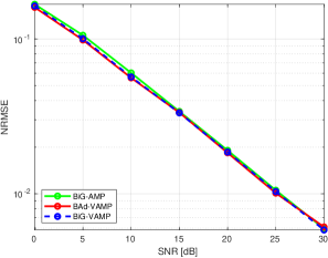
Figure 6: NRMSE of BiG-VAMP and BAd-VAMP vs. the SNR for the dictionary learning problem: Gaussian prior on $\boldsymbol{U}$, Bernoulli-Gaussian prior on $\boldsymbol{V}$ with a sparsity level of $95\%$, $N=1000$, $M=1000$, and $r=20$.

Note that BAd-VAMP was simulated with its defaults parameters from [23], i.e., $\tau_{1,\textrm{max}}=1$ and $\tau_{2,\textrm{max}}=0$, $\zeta=0.8$ and $\gamma_{\textrm{min}}=10^{-6}$. In Fig. 6, it is seen that BiG-AMP and BAd-VAMP exhibit the same performance as BiG-VAMP which is hardly surprising since all algorithms are optimally exploiting the considered priors on $\bm{U}$ and $\bm{V}$ and do not suffer from any convergence issues.
Next, we consider a binary prior on the unknown dictionary $\boldsymbol{U}$. Note that in this case the underlying dictionary learning problem is also known as the $\mathbb{Z}/2$ synchronization problem in the mathematical literature [28] or blind detection problem in the communication literature [29]. In this context, we again compare BiG-VAMP to BiG-AMP and we consider both low rank (i.e., $r=5$) and moderately high rank (i.e., $r=25$) structures as illustrated in Figs. 7 and 8, respectively.

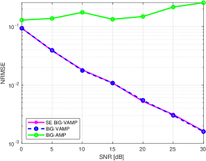
Figure 7: NRMSE of BiG-VAMP and BiG-AMP vs. the SNR for the dictionary learning problem: binary prior on $\boldsymbol{U}$, Bernoulli-Gaussian prior on $\boldsymbol{V}$ with a sparsity level of $95\%$, $N=100$, $M=100$ and $r=5$.

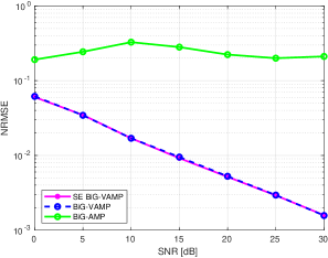
Figure 8: NRMSE of BiG-VAMP and BiG-AMP vs. the SNR for the dictionary learning problem: binary prior on $\boldsymbol{U}$, Bernoulli-Gaussian prior on $\boldsymbol{V}$ with a sparsity level of $95\%$, $N=500$, $M=500$ and $r=25$.

We do not include BAd-VAMP in the subsequent simulations since it is not designed to handlenon-Gaussian priors on $\boldsymbol{U}$ This is in fact due to the inherent limitation imposed by the combinatorial maximization step in the EM algorithm that BAd-VAMP uses to update $\boldsymbol{U}$ at every iteration.
Figs. 7 and 8 show order of-magnitude difference in the NRMSE performance of BiG-VAMP and BiG-AMP. While BiG-VAMP outperforms BiG-AMP under both low-rank and high-rank structures, the gap between the two algorithms is not inherently related to the rank value, but rather to the inablity of BiG-AMP to converge under discrete priors. Moreover, it is seen from both figures that the empirical NRMSE of BiG-VAMP is accurately predicted by the analytical state evolution recursion thereby corroborating the theoretical analysis we conducted in Section IV.

V-B Matrix factorization

In this case, we compare BiG-VAMP to BIG-AMP [26] for the case where $\boldsymbol{U}$ is a binary matrix and $\bm{V}$ is Gaussian-distributed. Fig. 9 depicts the NRMSE of both algorithms and reveals that BiG-AMP’s performance again deteriorates considerably in presence of a discrete prior either on $\bm{U}$ or $\bm{V}$ (due to the symmetry of the problem). BiG-VAMP, however, finds an accurate factorisation of $\bm{Z}$ over the entire SNR range and its empirical NRMSE is again theoretically predicted by the established state evolution analysis. This endows the proposed algorithm with offline design guidelines when applied to different engineering problems in practice.

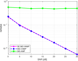
Figure 9: NRMSE of BiG-VAMP and BiG-AMP vs. the SNR for the matrix factorization problem: binary prior on $\boldsymbol{U}$, Gaussian prior on $\boldsymbol{V}$, $N=1000$, $M=200$ and $r=30$.

A close inspection of the NRMSE time evolution, as shown in Fig. 10, illustrates qualitatively a transiently chaotic trajectory that is similar to those of fluid parcels in turbulent flows studied in [ercsey2011optimization].Such a chaotic behaviour may be a generic feature of algorithms searching for solutions in hard optimization problems with applications as diverse as protein folding and Sudoku [elser2007searching].

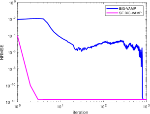
Figure 10: NRMSE of BiG-VAMP and its SE for the matrix factorization problem at $\textrm{SNR}=10$ dB: binary prior on $\boldsymbol{U}$, Gaussian prior on $\boldsymbol{V}$, $N=1000$, $M=500$ and $r=10$.

V-C Matrix completion

Unlike the previous two applications (i.e., matrix factorization and dictionary learning) wherein the observation model was linear, we now turn our attention to a popular generalized bilnear recovery problem, namely the matrix completion problem. In this context, Fig. 11 compares BiG-VAMP to BIG-AMP under the nonlinear observation model in (2) by taking $\phi(\cdot)$ to be a random selection with a rate of $20\%$. There, it is also seen that BiG-VAMP outperforms by far BiG-AMP which is in principle able to deal with any non-linearity in the observation model. But its deficiency here stems from the fact that it diverges for the considered challenging problem.

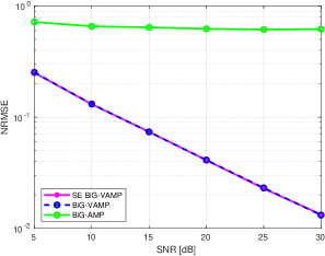
Figure 11: NRMSE of BiG-VAMP and BiG-AMP vs. the SNR for the matrix completion problem with a selection rate of $20\%$: binary prior on $\boldsymbol{U}$, Gaussian prior on $\boldsymbol{V}$, $N=1000$, $M=500$ and $r=30$.

For the case where the only problem structure available at hand is the low rank approximation, we also benchmark BiG-VAMP against LowRAMP [20] whose MATLAB code is publicly available from [30]. The results are depicted in Fig. 12 and as seen there LowRAMP is not able to correctly recover $\boldsymbol{U}$ and $\boldsymbol{V}$ while BiG-VAMP exhibits the same performance as BiG-VAMP. Under the considered non linear selection function, $\phi(\cdot)$, the performance degradation of LowRAMP is mainly due to the fact the second-order Taylor series approximation of the output channel (4), around $z_{ij}=0$, is not accurate high SNR values (which is a crucial condition to solve the matrix completion problem).

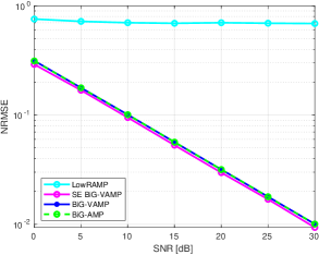
Figure 12: NRMSE of BiG-VAMP, BiG-AMP, and LowRAMP vs. the SNR for the matrix completion with the selection rate of $10\%$: Gaussian prior on $\bm{U}$, Gaussian prior on $\mathbf{V}$, $N=1000$, $M=500$ and $r=3$.

Fig. 13 shows the phase transition diagrams in the NRMSE for both low- and high-SNR regimes at a fixed selection rate of $20\%$. In the large-rank limit, we observe a low detectability regime when the SNR is in $[0,10]$ dB. This result is consistent with the non negligible uncertainty of estimators [31] to conduct inference in the low-SNR regime for noisy matrix completion.

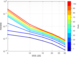
Figure 13: Phase transition diagram BiG-VAMP for the matrix completion problem with $N=1000$, $M=500$, $1\leq r\leq 100$, a selection rate of $20\%$, binary matrix $\mathbf{U}$ and Gaussian matrix $\boldsymbol{V}$.

VI Conclusion

In this work, we introduced a new algorithm, dubbed BiG-VAMP, to solve the generalized bilinear recovery problem based on the approximate message passing paradigm while treating both the MMSE and MAP inference problems in a unified framework. We described how BiG-VAMP provides a broader solution to the bilinear recovery problem under different structured matrices beyond the “low rank” structure heavily investigated in the existing literature. In particular, our numerical results for applications in matrix-factorization, dictionary learning, and matrix completion demonstrated that BiG-VAMP exhibits the best reconstruction performance under non Gaussian priors as compared to existing state-of-the-art algorithms such as BiG-AMP, BAd-VAMP, and LowRAMP. Additionally, we derived the state evolution equations of BiG-VAMP and characterized its phrase transition for the matrix completion problem.

References

- [1] R. Gribonval, R. Jenatton, and F. Bach, “Sparse and spurious: dictionary learning with noise and outliers,” IEEE Transactions on Information Theory, vol. 61, no. 11, pp. 6298–6319, 2015.
- [2] A. Montanari, Y. Eldar, and G. Kutyniok, “Graphical models concepts in compressed sensing,” Compressed Sensing: Theory and Applications, pp. 394–438, 2012.
- [3] H. Zou, T. Hastie, and R. Tibshirani, “Sparse principal component analysis,” Journal of computational and graphical statistics, vol. 15, no. 2, pp. 265–286, 2006.
- [4] Y. Koren, R. Bell, and C. Volinsky, “Matrix factorization techniques for recommender systems,” Computer, no. 8, pp. 30–37, 2009.
- [5] R. Matsushita and T. Tanaka, “Low-rank matrix reconstruction and clustering via approximate message passing,” in Advances in Neural Information Processing Systems, 2013, pp. 917–925.
- [6] L. Wang, Z. Zhang, and D. Dunson, “Symmetric bilinear regression for signal subgraph estimation,” IEEE Transactions on Signal Processing, vol. 67, no. 7, pp. 1929–1940, 2019.
- [7] Z. Lin, M. Chen, and Y. Ma, “The augmented lagrange multiplier method for exact recovery of corrupted low-rank matrices,” arXiv preprint arXiv:1009.5055, 2010.
- [8] S. Boyd, N. Parikh, E. Chu, B. Peleato, J. Eckstein et al., “Distributed optimization and statistical learning via the alternating direction method of multipliers,” Foundations and Trends® in Machine learning, vol. 3, no. 1, pp. 1–122, 2011.
- [9] S. D. Babacan, M. Luessi, R. Molina, and A. K. Katsaggelos, “Sparse bayesian methods for low-rank matrix estimation,” IEEE Transactions on Signal Processing, vol. 60, no. 8, pp. 3964–3977, 2012.
- [10] D. L. Donoho, A. Maleki, and A. Montanari, “Message-passing algorithms for compressed sensing,” Proceedings of the National Academy of Sciences, vol. 106, no. 45, pp. 18 914–18 919, 2009.
- [11] Y. C. Eldar and G. Kutyniok, Compressed sensing: theory and applications. Cambridge university press, 2012.
- [12] S. Rangan, “Generalized approximate message passing for estimation with random linear mixing,” in 2011 IEEE International Symposium on Information Theory Proceedings, 2011, pp. 2168–2172.
- [13] M. Bayati and A. Montanari, “The dynamics of message passing on dense graphs, with applications to compressed sensing,” IEEE Transactions on Information Theory, vol. 57, no. 2, pp. 764–785, 2011.
- [14] J. Barbier, F. Krzakala, N. Macris, L. Miolane, and L. Zdeborová, “Optimal errors and phase transitions in high-dimensional generalized linear models,” Proceedings of the National Academy of Sciences, vol. 116, no. 12, pp. 5451–5460, 2019.
- [15] M. Mezard and A. Montanari, Information, physics, and computation. Oxford University Press, 2009.
- [16] S. Rangan, P. Schniter, and A. K. Fletcher, “Vector approximate message passing,” in 2017 IEEE International Symposium on Information Theory (ISIT), 2017, pp. 1588–1592.
- [17] P. Schniter, S. Rangan, and A. K. Fletcher, “Vector approximate message passing for the generalized linear model,” in 2016 50th Asilomar Conference on Signals, Systems and Computers. IEEE, 2016, pp. 1525–1529.
- [18] S. Rangan, P. Schniter, and A. K. Fletcher, “Vector approximate message passing,” IEEE Transactions on Information Theory, vol. 65, no. 10, pp. 6664–6684, 2019.
- [19] J. Ma and L. Ping, “Orthogonal amp,” IEEE Access, vol. 5, pp. 2020–2033, 2017.
- [20] T. Lesieur, F. Krzakala, and L. Zdeborová, “Phase transitions in sparse pca,” in 2015 IEEE International Symposium on Information Theory (ISIT). IEEE, 2015, pp. 1635–1639.
- [21] J. T. Parker, P. Schniter, and V. Cevher, “Bilinear generalized approximate message passing—part i: Derivation,” IEEE Transactions on Signal Processing, vol. 62, no. 22, pp. 5839–5853, 2014.
- [22] J. T. Parker and P. Schniter, “Parametric bilinear generalized approximate message passing,” IEEE Journal of Selected Topics in Signal Processing, vol. 10, no. 4, pp. 795–808, 2016.
- [23] S. Sarkar, A. K. Fletcher, S. Rangan, and P. Schniter, “Bilinear recovery using adaptive vector-amp,” IEEE Transactions on Signal Processing, vol. 67, no. 13, pp. 3383–3396, 2019.
- [24] A. P. Dempster, N. M. Laird, and D. B. Rubin, “Maximum likelihood from incomplete data via the em algorithm,” Journal of the Royal Statistical Society: Series B (Methodological), vol. 39, no. 1, pp. 1–22, 1977.
- [25] A. M. Tulino, S. Verdú et al., “Random matrix theory and wireless communications,” Foundations and Trends® in Communications and Information Theory, vol. 1, no. 1, pp. 1–182, 2004.
- [26] P. Schniter, “BiGAMP.” [Online]. Available: https://sourceforge.net/projects/gampmatlab/
- [27] S. Sarkar, “Bilinear Adaptive Vector Approximate Message Passing,” Jul. 2019. [Online]. Available: https://github.com/sbrsarkar/BAdVAMP
- [28] A. Perry, A. Wein, A. Bandeira, and A. Moitra, “Message-Passing Algorithms for Synchronization Problems over Compact Group,” Communications on Pure and Applied Mathematics, 10 2016.
- [29] A. Mezghani and A. L. Swindlehurst, “Blind Estimation of Sparse Broadband Massive MIMO Channels With Ideal and One-bit ADCs,” IEEE Transactions on Signal Processing, vol. 66, no. 11, pp. 2972–2983, 2018.
- [30] F. Krzakala, “Low rank Matrix Factorization with AMP,” Aug. 2015. [Online]. Available: https://github.com/krzakala/LowRAMP
- [31] Y. Chen, J. Fan, C. Ma, and Y. Yan, “Inference and uncertainty quantification for noisy matrix completion,” Proceedings of the National Academy of Sciences, vol. 116, no. 46, pp. 22 931–22 937, 2019.