Nonequilibrium phases and phase transitions of the XY-model

Abstract

We obtain the steady-state phase diagram of a transverse field XY spin chain coupled at its ends to magnetic reservoirs held at different magnetic potentials. In the long-time limit, the magnetization bias across the system generates a current-carrying non-equilibrium steady-state. We characterize the different non-equilibrium phases as functions of the chain’s parameters and magnetic potentials, in terms of their correlation functions and entanglement content. The mixed-order transition, recently observed for the particular case of a transverse field Ising chain, is established to emerge as a generic out-of-equilibrium feature and its critical exponents are determined analytically. Results are also contrasted with those obtained in the limit of Markovian reservoirs. Our findings should prove helpful in establishing the properties of non-equilibrium phases and phase transitions of extended open quantum systems.

I Introduction

Quantum matter out of thermal equilibrium has become a central research topic in recent years. An important class of problems deal with non-equilibrium quantum states of systems that are in contact with multiple baths which in turn are held at specified thermodynamic potentials. Such states are not bounded by equilibrium fluctuation relations and thus may host phases of matter that are impossible to realize in equilibrium. Therefore, phase changes far from equilibrium may exist that lack equilibrium counterparts.

Far-from-equilibrium quantum states are routinely realized in mesoscopic solid-state devices Pothier et al. (1997); Anthore et al. (2003); Chen et al. (2009) and recently have also become available in cold atomic gas settings Brantut et al. (2013). It thus is timely to explore the properties of phases of current-carrying matter and address the conditions which have to be met for their emergence.

Non-equilibrium transport across quantum materials dates back to Landauer and Büttiker Büttiker and Landauer (1982), who were motivated by the failure of semi-classical Boltzmann-like approaches to understand phenomena such as the conductance quantization across mesoscopic conductors. For non-interacting systems, quantum transport is by now well understood Stefanucci and van Leeuwen (2013); Datta et al. (1997); Imry (2002). However, in systems where the physical properties are determined by the electron-electron interaction, progress has been much slower. Here, one often has to resort to either approximate methods or numerically exact techniques Aoki et al. (2014) which, however, are often restricted to small systems or comparatively high temperatures. Exact analytical results, available for integrable models in one dimension, do not typically generalize to open setups. Moreover, non-thermal steady-states in Luttinger liquids Gutman et al. (2008, 2009); Ngo Dinh et al. (2010), seem to be less general than their equilibrium counterparts.

Considerable progress has been made in the Markovian case, where the environment lacks memory Prosen and Pižorn (2008); Prosen and Žunkovič (2010); Prosen (2011, 2014). The applicability of the Markovian case is, however, limited to extreme non-equilibrium conditions (e.g., very large bias or temperature) and is of restricted use for realistic transport setups Ribeiro and Vieira (2015a, b).

Other recent developments to study transport include, the study of so-called generalized hydrodynamic methods available for integrable systems Bertini et al. (2016); Castro-Alvaredo et al. (2016) and hybrid approaches involving Lindblad dynamics Arrigoni et al. (2013). However, these methods are not yet able to describe current-carrying steady-states in extended mesoscopic systems.

Our recent analysis of the exactly solvable transverse field Ising chain attached to macroscopic reservoirs has allowed us study a symmetry-breaking quantum phase transition in the steady-state of an extended non-equilibrium system Puel et al. (2019). At the equilibrium level, this model can be mapped onto that of non-interacting fermions via a Jordan-Wigner transformation and is thus solvable by elementary means.

The non-thermal steady-state of this model is, however, much richer and allows for a peculiar symmetry-breaking quantum phase transition. In particular, we have shown that this transition to be of mixed-order (or hybrid) nature, with a discontinuous order parameter and diverging correlation length. This type of transitions were first discussed by Thouless in 1969 (Thouless, 1969) in the context of classical spin chains with long-range interactions and have since then reported in different environments (Bar and Mukamel, 2014; Fronczak et al., 2016; Anglès d’Auriac and Iglói, 2016; Juhász and Iglói, 2017; Alert et al., 2017).

Even though realistic systems are only approximately described by exactly solvable models at best, exact solutions are still of considerable value. Not only can they be important in unveiling features of novel effects but they are commonly instrumental in benchmarking numerical and approximate methods. Therefore, exact solutions are particularly helpful in situations where no reliable numerical or approximate methods yet exist, such as in the description of current-carrying steady-states of interacting systems.

In this article, we provide a set of exact results of steady-state phases and phase transitions of an $XY$ spin chain in a transverse field coupled to magnetic reservoirs held at different magnetizations. Our analysis extends and generalizes the findings in Ref. [Puel et al., 2019] and points out new regimes that are not present in the Ising case. In the Markovian limit, we recover previous results obtained for $XY$ spin chains coupled to free-of-memory reservoirs (Prosen and Pižorn, 2008; Žunkovič and Prosen, 2010; Ajisaka et al., 2014) where an out-of-equilibrium phase transition with spontaneous emergence of long-range order has been found.

The paper is organized as follows. In section II we define the out-of-equilibrium model and briefly describe the methods used to solve it. In section III we describe in detail the non-equilibrium phase diagram based on the energy current and the properties of the occupation number. The correlation functions in the various phases are analysed in section IV, where we also discuss the critical behavior at the mixed-order phase transition and the characteristic oscillations in the $z$-correlation function. Universal features of the entanglement entropy are discussed in section V. Finally, we summarize and conclude our work in section VI.

II Model and Method

II.1 Hamiltonian and Jordan-Wigner mapping

We consider an $XY$-spin chain of $N$ sites (labeled by $r$), exchange coupling $J$, and coupled to a transverse field $h$. At its ends, i.e., at $r=1$ and $r=N$, the chain is coupled to magnetic reservoirs which are kept at zero temperature ($T=0$). The Hamiltonian of the chain is given by

$${\cal H}_{\text{C}}= -\frac{J}{2}\sum_{r=1}^{N-1}\left(\left(1+\gamma\right)\sigma_{r}^{x}\sigma_{r+1}^{x}+\left(1-\gamma\right)\sigma_{r}^{y}\sigma_{r+1}^{y}\right)$$

$$-h\sum_{r=1}^{N}\sigma_{r}^{z},$$ (1)

where $\sigma_{r}^{x,y,z}$ are the Pauli matrices at site $r$, and $\gamma$ controls the anisotropy. The total Hamiltonian is given by

$${\cal H}={\cal H}_{\text{C}}+\sum_{l=\text{L},\text{R}}\left({\cal H}_{l}+{\cal H}_{\text{C-}l}\right),$$ (2)

where ${\cal H}_{l}$ and ${\cal H}_{\text{C-}l}$, with $l=\text{L,R}$, are respectively the Hamiltonians of the reservoirs and the system-reservoir coupling terms. In the following, we assume that the reservoirs possess bandwidths which are entirely determined by magnetic potential $\mu_{l}$ ($l=\text{L,R}$) and which are much larger than the energy scales that characterize the chain.

In the wide-band limit, results become independent of the details of ${\cal H}_{l}$ and ${\cal H}_{\text{C-}l}$. For concreteness, we take the reservoirs to be isotropic $XY-$chains, i.e.

$${\cal H}_{l}=-J_{l}\sum_{r_{l}\in\Omega_{l}}\left(\sigma_{r_{l}}^{x}\sigma_{r_{l}+1}^{x}+\sigma_{r_{l}}^{y}\sigma_{r_{l}+1}^{y}\right),$$ (3)

with $l=\text{L},\text{R}$, and we have defined $\Omega_{\text{L}}\equiv\left\{-\infty,\ldots,0\right\}$, $\Omega_{\text{R}}\equiv\left\{N+1,\ldots,\infty\right\}$. Initially, the reservoirs are in an equilibrium Gibbs state, $\rho_{l}=e^{-\beta(\mathcal{H}_{l}-\mu_{l}M_{l})}$, where $M_{l}=\sum_{r_{l}\in\Omega_{l}}\sigma_{r_{l}}^{z}$ is the reservoir magnetization (which is a good quantum number in the absence of system-reservoir coupling, i.e., $\left[{\cal H}_{l},M_{l}\right]=0$). The average value of $M_{l}$ is set by the magnetic potential $\mu_{l}$. For finite $\mu_{l}$ these are non-Markovian reservoirs, with power-law decaying correlations, and a set of gapless magnetic excitations within an energy bandwidth $J_{l}\gg J,h$. The chain-reservoir coupling Hamiltonians are

$${\cal H}_{\text{C-}l}=-J_{\text{C-}l}\left(\sigma_{\left(r_{l}\right)_{\text{C}}}^{x}\sigma_{\left(r\right)_{l}}^{x}+\sigma_{\left(r\right)_{l}}^{y}\sigma_{\left(r_{l}\right)_{\text{C}}}^{y}\right),$$ (4)

with $\left(r_{\text{L}}\right)_{\text{C}}=1$, $\left(r\right)_{\text{L}}=0$, $\left(r_{\text{R}}\right)_{\text{C}}=N$, and $\left(r\right)_{\text{R}}=N+1$. A sketch of this system is shown in Fig.1(a).

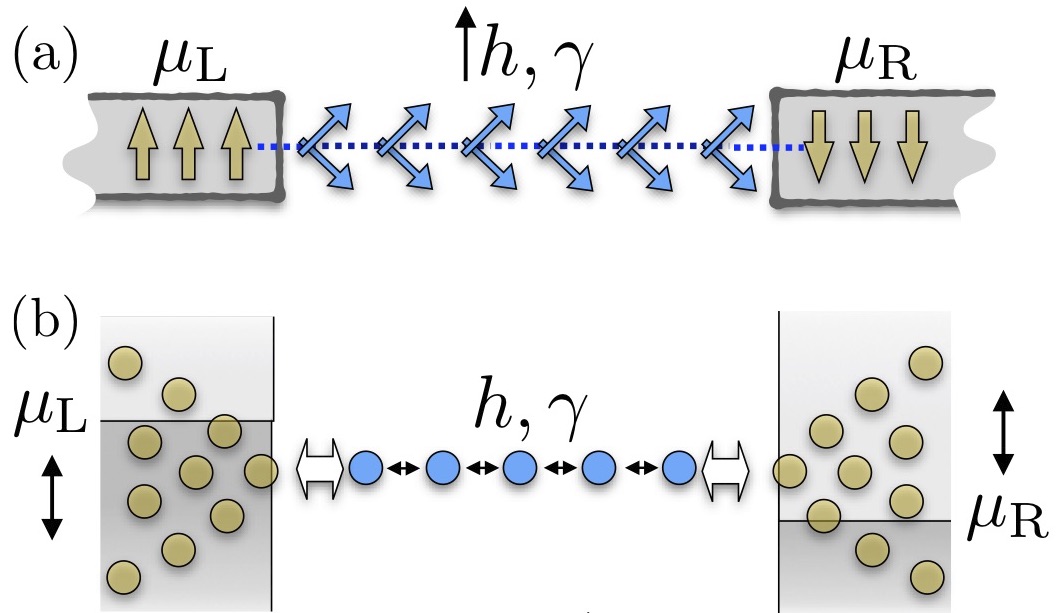
Figure 1: (a) Schematic picture of the XY-model spin chain in contact with magnetic reservoirs and (b) the same system mapped to its fermionic representation, i.e. a triplet superconducting chain of spinless fermions in contact with fermionic reservoirs.

The full Hamiltonian, ${\cal H}$, can be represented in terms of fermions via the so-called Jordan-Wigner (JW) mapping(Lieb et al., 1961a), $\sigma_{r}^{+}=e^{i\pi\sum_{r^{\prime}=1}^{r-1}\hat{c}_{r^{\prime}}^{\dagger}\hat{c}_{r^{\prime}}}c_{r}^{\dagger}$, where $\hat{c}_{r}^{\dagger}/\hat{c}_{r}$ creates/annihilates a spinless fermion at site $r$. The JW-transformed system corresponds to a Kitaev chain(Kitaev, 2001) in contact with two metallic reservoirs of spinless fermions at chemical potentials $\mu_{\text{L},\text{R}}$, i.e.

$${\cal H}=-J\sum_{r=1}^{N-1}\left(\hat{c}_{r}^{\dagger}\hat{c}_{r+1}+\gamma\hat{c}_{r}^{\dagger}\hat{c}_{r+1}^{\dagger}+\text{h.c.}\right)-2h\sum_{r=1}^{N}\hat{c}_{r}^{\dagger}\hat{c}_{r}$$

$$-\sum_{l=\text{L,R}}\left[J_{\text{C-}l}\hat{c}_{\left(r_{l}\right)_{\text{C}}}^{\dagger}\hat{c}_{\left(r\right)_{l}}+J_{l}\sum_{r_{l}\in\Omega_{l}}\hat{c}_{r_{l}}^{\dagger}\hat{c}_{r_{l}+1}+\text{h.c.}\right],$$ (5)

where $J\gamma$ defines the superconducting coupling strength and $h$ plays the role a potential applied on the chain. A sketch of this system is shown in Fig.1(b). In equilibrium, topologically non-trivial phases of the Kitaev chain correspond to magnetically ordered phases of the original XY-spin model, whereas the topologically trivial cases correspond to disordered phases. With a magnetic bias, the transfer of spin excitations between the reservoirs was studied rather extensively (see, e.g., Refs. Meier and Loss, 2003; Nakata et al., 2017), also considering transport signatures of the topological phase in short junctions.Hoffman et al. (2018); Shen et al. (2020) Here, however, we will be mostly concerned with the bulk properties at $N\to\infty$, and after the reservoirs have been traced out.

II.2 Non-equilibrium Green’s functions

As the JW-transformed Hamiltonian is quadratic in its fermionic degrees of freedom, the non-equilibrium system admits an exact solution in terms of single-particle quantities. In the following, we employ the non-equilibrium Green’s function formalism to compute correlation functions and related observables. The procedure is described in the Supplemental Material of Ref. [Puel et al., 2019] and is briefly summarized here for convenience.

We start by defining the Nambu vector, $\hat{\boldsymbol{\Psi}}^{\dagger}=\left(\hat{c}_{1}^{\dagger},\ldots,\hat{c}_{N}^{\dagger},\hat{c}_{1},\ldots,\hat{c}_{N}\right)$, and the retarded, advanced, and Keldysh components of the Green’s function, given by

$$\boldsymbol{G}^{R}_{i,j}(t-t^{\prime}) = -i\Theta\left(t-t^{\prime}\right)\left\langle\left\{\hat{\boldsymbol{\Psi}}_{i}(t),\hat{\boldsymbol{\Psi}}_{j}^{\dagger}(t^{\prime})\right\}\right\rangle,$$ (6)

$$\boldsymbol{G}^{A}_{i,j}(t-t^{\prime}) = i\Theta\left(t^{\prime}-t\right)\left\langle\left\{\hat{\boldsymbol{\Psi}}_{i}(t),\hat{\boldsymbol{\Psi}}_{j}^{\dagger}(t^{\prime})\right\}\right\rangle,$$ (7)

$$\boldsymbol{G}^{K}_{i,j}(t-t^{\prime}) = -i\left\langle\left[\hat{\boldsymbol{\Psi}}_{i}(t),\hat{\boldsymbol{\Psi}}_{j}^{\dagger}(t^{\prime})\right]\right\rangle.$$ (8)

Using this notation, the Hamiltonians for the right, left reservoirs and for the chain are given by ${\cal H}_{l}=\frac{1}{2}\hat{\boldsymbol{\Psi}}^{\dagger}\boldsymbol{H}_{l}\hat{\boldsymbol{\Psi}}$, with $l=\text{L,R,C}$. For the chain, $\boldsymbol{H}_{\text{C}}$ is a $2N\times 2N$ Hermitian matrix respecting particle-hole symmetry, i.e., $\boldsymbol{S}^{-1}\boldsymbol{H}_{\text{C}}^{T}\boldsymbol{S}=-\boldsymbol{H}_{\text{C}}$ where $\boldsymbol{S}=\tau^{x}\otimes\boldsymbol{1}_{N\times N}$ and $\tau^{x}$ interchanges particle and hole spaces. Similar definitions apply to the degrees of freedom of the right and left reservoirs. The bare retarded and advanced Green’s functions, in the absence of chain-reservoir couplings, are simply given by $\boldsymbol{G}_{l,0}^{R/A}\left(\omega\right)=\left(\omega-\boldsymbol{H}_{l}\pm i\eta\right)^{-1}$. Re-writing the chain-reservoir coupling in the same notation, ${\cal H}_{\text{C-}l}=\frac{1}{2}\left(\hat{\boldsymbol{\Psi}}^{\dagger}_{(l)}\boldsymbol{T}\hat{\boldsymbol{\Psi}}+\hat{\boldsymbol{\Psi}}^{\dagger}\boldsymbol{T}^{\dagger}\hat{\boldsymbol{\Psi}}_{(l)}\right)$. The self-energy of the chain, induced by tracing out the reservoirs, are $\boldsymbol{\Sigma}^{R/A/K}=\sum_{l=\text{L,R}}\boldsymbol{\Sigma}^{R/A/K}_{l}$ where

$$\boldsymbol{\Sigma}^{R/A}_{l}(\omega) = \boldsymbol{T}^{\dagger}\boldsymbol{G}_{l,0}^{R/A}(\omega)\boldsymbol{T},$$ (9)

$$\boldsymbol{\Sigma}_{l}^{K}(\omega) = \left[\boldsymbol{\Sigma}_{l}^{R}(\omega)-\boldsymbol{\Sigma}_{l}^{A}(\omega)\right]\left[1-2n_{\mathrm{F},l}(\omega)\right],$$ (10)

are the contributions of reservoir $l$, which obey equilibrium fluctuation-dissipation relations, and where $n_{\text{F},l}(\omega)=(e^{\beta_{l}(\omega-\mu_{l})}+1)^{-1}$ is the Fermi-function with chemical potential $\mu_{l}$ and inverse temperature $\beta_{l}$. The chain steady-state Green’s functions are obtained from the Dyson’s equation,

$$\boldsymbol{G}_{\text{C}}^{R/A}(\omega) = \left[\boldsymbol{G}_{\text{C},0}^{R/A}(\omega)-\boldsymbol{\Sigma}^{R/A}(\omega)\right]^{-1},$$ (11)

$$\boldsymbol{G}_{\text{C}}^{K}(\omega) = \boldsymbol{G}_{\text{C}}^{R}(\omega)\boldsymbol{\Sigma}^{K}(\omega)\boldsymbol{G}_{\text{C}}^{A}(\omega).$$ (12)

As mentioned above, we consider the case where the bandwidths of the reservoirs, $J_{l=\text{L},\text{R}}$ are much larger than the other energy scales. In this wide band limit, the coupling to reservoir $l$ is completely determined by the hybridization energy scale $\Gamma_{l}=\pi J_{\text{C-}l}^{2}D_{l}$. Here, $D_{l}$ is the reservoir’s constant-local density of states. In practice, the wide band limit yields a frequency independent retarded self-energy, $\boldsymbol{\Sigma}^{R}_{l}=i(\boldsymbol{\gamma}_{l}+\bar{\boldsymbol{\gamma}}_{l})$, which substantially simplifies subsequent calculations, with $\boldsymbol{\gamma}_{l}=\Gamma_{l}\left|r_{l}\right\rangle\left\langle r_{l}\right|$ and $\bar{\boldsymbol{\gamma}}_{l}=\Gamma_{l}\left|\bar{r}_{l}\right\rangle\left\langle\bar{r}_{l}\right|$, and where $\left|r\right\rangle$ and $\left|\bar{r}\right\rangle\equiv\boldsymbol{S}\left|r\right\rangle$ are single-particle and hole states.

In this case, it is convenient to define the non-Hermitian single-particle operator

$$\boldsymbol{K}\equiv\boldsymbol{H}_{\text{C}}-i\sum_{l=\text{L,R}}\left(\boldsymbol{\gamma}_{l}+\bar{\boldsymbol{\gamma}}_{l}\right),$$ (13)

which we assume to be diagonalizable, possessing right and left eigenvectors $\left|\alpha\right\rangle$ and $\left\langle\tilde{\alpha}\right|$, and associated eigenvalues $\lambda_{\alpha}$. In terms of these quantities, the retarded Green’s function is given by

$$\boldsymbol{G}^{R}\left(\omega\right)=\left(\omega-\boldsymbol{K}\right)^{-1}=\sum_{\alpha}\left|\alpha\right\rangle\left(\omega-\lambda_{\alpha}\right)^{-1}\left\langle\tilde{\alpha}\right|,$$ (14)

and the Keldysh Green’s function becomes

$$\boldsymbol{G}^{K}\left(\omega\right)=-2i\sum_{l}\sum_{\alpha\beta}\left|\alpha\right\rangle\left\langle\beta\right|\times$$

$$\frac{\left\langle\alpha^{\prime}\right|\boldsymbol{\gamma}_{l}\left|\beta^{\prime}\right\rangle\left[1-2n_{\text{F},l}\left(\omega\right)\right]-\left\langle\alpha^{\prime}\right|\bar{\boldsymbol{\gamma}}_{l}\left|\beta^{\prime}\right\rangle\left[1-2n_{\text{F},l}\left(-\omega\right)\right]}{\left(\omega-\lambda_{\alpha}\right)\left(\omega-\bar{\lambda}_{\beta}\right)}.$$ (15)

Steady-state observables can be obtained from the single-particle correlation function matrix, $\boldsymbol{\chi}\equiv\langle\hat{\boldsymbol{\Psi}}\hat{\boldsymbol{\Psi}}^{\dagger}\rangle$, which is obtained from the Keldysh Green’s function

$$\boldsymbol{\chi}=\frac{1}{2}\left[i\int\frac{d\omega}{2\pi}\boldsymbol{G}^{K}\left(\omega\right)+\boldsymbol{1}\right].$$ (16)

The explicit form of $\boldsymbol{\chi}$ after performing the integration over frequencies is provided in Eq.(41). As the model is quadratic, $\boldsymbol{\chi}$ encodes all the information about the reduced density matrix of the chain, $\hat{\rho}_{\text{C}}=\text{tr}_{\text{L,R}}[\hat{\rho}]$. This quantity can itself be expressed as the exponential of a quadratic operator, i.e. $\hat{\rho}_{\text{C}}=\text{e}^{\hat{\Omega}_{\text{C}}}/Z$, where $Z=\text{tr}\left[\text{e}^{\hat{\Omega}_{\text{C}}}\right]$ and $\hat{\Omega}_{\text{C}}=\frac{1}{2}\hat{\boldsymbol{\Psi}}^{\dagger}\boldsymbol{\Omega}_{\text{C}}\hat{\boldsymbol{\Psi}}$ with $\boldsymbol{\Omega}_{\text{C}}$ being a $2N\times 2N$ matrix respecting the particle-hole symmetry conditions. $\hat{\Omega}_{\text{C}}$ is related to the single-particle density matrix via

$$\boldsymbol{\chi}=\left(\text{e}^{\boldsymbol{\Omega}_{\text{C}}}+\boldsymbol{1}\right)^{-1}.$$ (17)

This relation allows the calculation of mean values of quadratic observables, $\hat{O}=\frac{1}{2}\hat{\boldsymbol{\Psi}}^{\dagger}\boldsymbol{O}\hat{\boldsymbol{\Psi}}$, defined by the Hermitian and particle-hole symmetric matrix $\boldsymbol{O}$,

$$\left\langle\hat{O}\right\rangle=\text{Tr}\left[\hat{\rho}_{\text{C}}\hat{O}\right]=-\frac{1}{2}\text{tr}\left[\boldsymbol{O}\cdot\boldsymbol{\chi}\right],$$ (18)

as well as all higher-order correlation functions.

III Phase diagram

This section discusses the non-equilibrium phase diagram of the model, as well as the excitations and associated occupation numbers in the various different phases. To contextualize our findings, the first two sub-sections are devoted to a brief description of the equilibrium properties of the $XY$-chain and a review of the non-equilibrium Markovian limit.

III.1 Equilibrium phases

The system in equilibrium is more conveniently studied without considering the couplings to the leads and assuming periodic boundary conditions. After performing the JW transformation, the Hamiltonian of the translation-invariant chain is diagonalized in the momentum representation by a suitable Bogoliubov transformation, i.e., ${\cal H}_{C}=\sum_{k}\varepsilon_{k}(\hat{\gamma}_{k}^{\dagger}\hat{\gamma}_{k}-1/2)$, where the operators $(\hat{\gamma}_{k},\hat{\gamma}_{-k}^{\dagger})^{T}=e^{i\theta_{k}\sigma_{x}}(\hat{c}_{k},\hat{c}_{-k}^{\dagger})^{T}$ describe excitations of energy

$$\varepsilon_{k}=2J\sqrt{\left(h/J+\cos k\right)^{2}+\left(\gamma\sin k\right)^{2}},$$ (19)

and $\sin\left(2\theta_{k}\right)=-2J\gamma\sin(k)/\varepsilon_{k}$.

The ground state is characterized by a vanishing number of Bogoliubov excitation, i.e., $n_{k}=0$ where

$$n_{k}\equiv\langle\hat{\gamma}_{k}^{\dagger}\hat{\gamma}_{k}\rangle.$$ (20)

For $\left|h/J\right|<1$, the ground-state is topologically non-trivial with positive and negative anisotropies ($\gamma>0$ or $<0$) corresponding to opposite signs of the topological invariant, separated by a critical gapless state for $\gamma=0$. At $\left|h/J\right|=1$, the spectral gap vanishes and the system transitions into a topologically trivial phase at large $h$.

A similar phase diagram is obtained in terms of the original spin degrees of freedom. Fig. 2(a) illustrates the zero-temperature phase diagram of the equilibrium $XY$-model. For $\gamma>0$, the systems is magnetically ordered along the $x$ direction under a weak transverse field, $h$, and possesses a finite magnetization(Barouch and McCoy, 1971) $\phi\equiv\lim_{h_{x}\to 0}\lim_{L\to\infty}\frac{1}{N}\sum_{r}\left\langle\sigma^{x}_{r}\right\rangle\neq 0$, where $h_{x}$ is a symmetry-breaking magnetic field along the $x$ direction. A negative anisotropy, i.e., $\gamma<0$, yields a non-vanishing magnetization along the $y$ direction, whereas at $\gamma=0$ the system is critical and isotropic for $\left|h/J\right|<1$. As the ordered phases for $\gamma>0$ and $<0$ are equivalent to each other and related via a simple rotation, only $\gamma>0$ is considered in the subsequent analysis. It is worth recalling that the special cases $\gamma=\pm 1$ correspond to the transverse field Ising model. A strong $h$ drives the magnetic phase through a second order phase transition into a phase of vanishing magnetization, i.e., a phase with $\phi=0$. Near the transition, for $\left|h/J\right|<1$, the magnetization behaves as $\phi\simeq\sqrt{\frac{2}{1+|\gamma|}}\left\{\gamma^{2}\left[1-\left(h/J\right)^{2}\right]\right\}^{1/8}$ Barouch and McCoy (1971).

The computation of the order parameter, $\phi$, directly from the above definition is not possible via the JW mapping. Instead one considers the two-points correlation functions ($\alpha=x,y,z$):

$$\mathbb{C}_{r,r^{\prime}}^{\alpha\alpha}=\langle\sigma_{r}^{\alpha}\sigma_{r^{\prime}}^{\alpha}\rangle-\langle\sigma_{r}^{\alpha}\rangle\langle\sigma_{r^{\prime}}^{\alpha}\rangle.$$ (21)

For disordered phases in equilibrium, these correlators are expected to show either exponential (EXP) or power-law (PL) decay depending on whether the system is gapped or gapless. In the ordered phase the system has long-range order (LRO) correlations, e.g., for $\gamma>0$,

$$\mathbb{C}_{r,r^{\prime}}^{xx}\simeq A\text{e}^{-\left|r-r^{\prime}\right|/\xi}+\phi^{2},$$ (22)

where $\xi$ is the characteristic correlation length and $A$ a numeric coefficient. This expression allows one to obtain $\phi$ from the correlation function $\mathbb{C}_{r,r^{\prime}}^{xx}$, which in turn can be computed in terms of a Toeplitz determinant (Lieb et al., 1961b; Sachdev, 1996). In equilibrium, all correlation functions, except $\mathbb{C}_{r,r^{\prime}}^{xx}$, either vanish or decay exponentially with $\left|r-r^{\prime}\right|$.

For an open system connected to demagnetized baths, i.e., $\mu_{L,R}=0$, the same equilibrium bulk properties as those for the closed system are found. It is natural to expect that bulk properties pertain for distances greater than $\xi$ away from the leads. Our calculation of fermionic observables follows that described in Sec.II. The calculation of the spin-spin correlation functions are similar to those for the translation-invariant system and is given in Appendix A in terms of the single-particle correlation matrix $\boldsymbol{\chi}$.

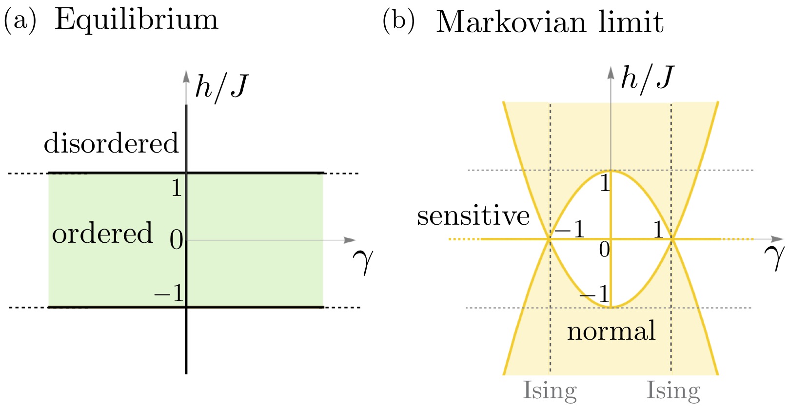
Figure 2: (a) Phase diagram $h/J\times\gamma$ of the XY-model in equilibrium. The black-thick lines identify a gap closing. (b) Phase diagram of the out-of-equilibrium XY-model according to the presence (sensitive) or absence (normal) of long-range correlations in the Markovian limit. The vertical dashed line at $\gamma=+1$ $(\gamma=-1)$ identifies the Ising model with only XX(YY)-spin-coupling interactions.

III.2 Nonequilibrium phases in the Markovian limit

The non-equilibrium features of the XY-model with Markovian reservoirs were first reported in Refs. [Prosen and Pižorn, 2008; Banchi et al., 2014]. This limit can be recovered from the present model by taking $\left|\mu_{\text{R}}\right|$ or $\left|\mu_{\text{L}}\right|\rightarrow\infty$(Ribeiro and Vieira, 2015a). The steady-state phase diagram in that limit possesses two distinct phases characterized respectively by an exponential decay of all correlation functions with distance and by an algebraic decay of $\mathbb{C}^{zz}_{r,r^{\prime}}$ concomitant with a strong sensitivity to small variations of some control parameters(Prosen and Pižorn, 2008). Fig. 2(b) depicts the phase diagram in this Markovian limit and with its sensitive (white) and normal (light-yellow) phases. The dark yellow lines mark critical phase boundaries.

The quasiparticle dispersion relation, given by Eq.(19), is shown in 3(a) and (c). The algebraic correlations are associated to the presence of an inflection point in the quasiparticle dispersion which appears for $h/J\leq|1-\gamma^{2}|$. In the normal region, the extrema of the energy are $m_{1}=\varepsilon_{k=0}=2J\left|1+h/J\right|$ and $m_{2}=\varepsilon_{k=\pi}=2J\left|1-h/J\right|$, while for the sensitive region $m_{3}=2J\left|\gamma\right|\sqrt{1+\left(h/J\right)^{2}\left(\gamma^{2}-1\right)^{-1}}$ becomes a global extremum. Figs. 3(b) and 3(d) show the spectrum of the non-Hermitian single-particle operator $\boldsymbol{K}$ (see Eq. (13)) for both normal and sensitive phases. It turns out that the imaginary part of the eigenvalues scales with the inverse system size, $\text{Im}\lambda_{\alpha}\propto N^{-1}$. (Medvedyeva and Kehrein, 2014) This is a reflection of the fact that for the chain degrees of freedom, the dissipative effects of the boundary become less important with increasing system size. A key feature of the sensitive region is that, for energies (i.e. $\text{Re}(\lambda_{\alpha})$) where four momenta can propagate, the spectrum does not converge to a line with increasing system size, but becomes scattered within a finite area (Prosen and Pižorn, 2008). These effects are independent of the Markovian nature of the reservoirs and remain for the non-Markovian case as the operator $\boldsymbol{K}$ does not depend on the chemical potential of the leads. Thus, as explicitly shown below, the normal-sensitive transition, reported in Refs. [Prosen and Pižorn, 2008; Banchi et al., 2014] for the Markovian case, also occurs for finite values of $\mu_{\text{L}}$ and $\mu_{\text{R}}$.

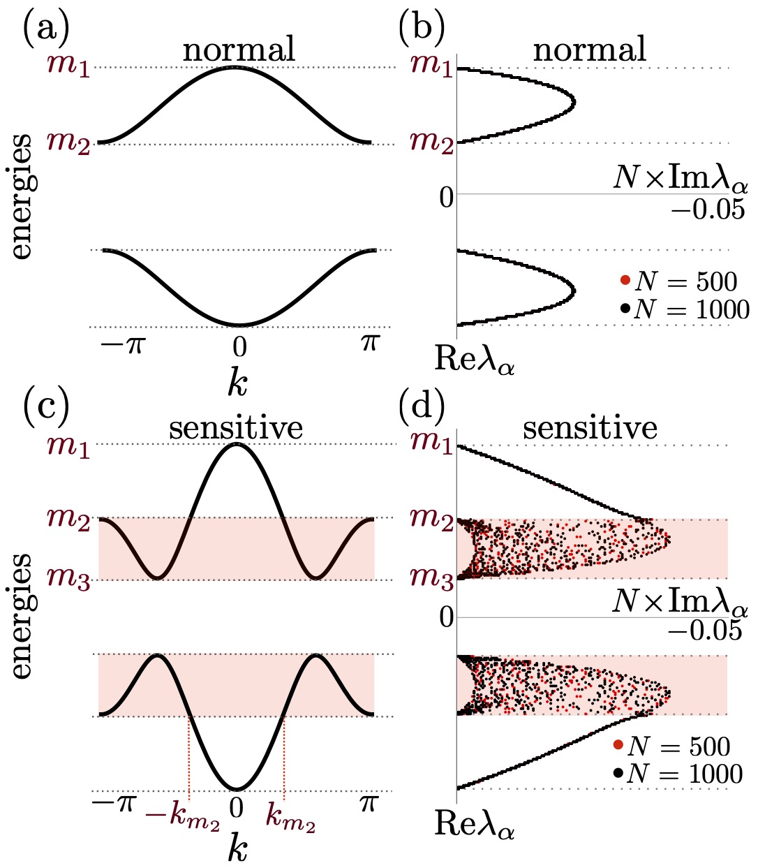
Figure 3: Quasiparticle dispersion relation of the equilibrium XY-model in the normal (a) and sensitive (c) regions, with $\{\gamma,h/J\}=\{1.0,0.2\}$ and $\{\gamma,h/J\}=\{0.5,0.2\}$ respectively, which leads to $\{m_{1},m_{2},m_{3}\}=\{2.4,1.6,0.97\}$. $\pm k_{m_{2}}$ are the two momenta with energy $m_{2}$. (b) and (d) depict the eigenvalues $\lambda_{\alpha}$ of the non-Hermitian single-particle operator $\boldsymbol{K}$ in the complex plane.

III.3 Non-equilibrium phase diagram - energy current

We now present the phase diagram of non-equilibrium $XY$ model and show that the energy current passing through the chain can be used to discriminate between the different phases.

Conservation of energy implies that the steady-state energy current is equal across any cross section along the chain and can be obtained from $\boldsymbol{\chi}$ as

$$\mathcal{J}_{e}=-\frac{1}{2}\,\text{tr}\left[\boldsymbol{J}_{r}\cdot\boldsymbol{\chi}\right],$$ (23)

where $\boldsymbol{J}_{r}$ is the single-particle current operator at link $(r,r+1)$ which is explicitly given in Appendix A.

We have previously discussed the steady-state energy current in a non-Markovian setting for the particular case of the transverse field Ising model, i.e., $\left|\gamma\right|=1$, in Ref. [Puel et al., 2019]. The non-equilibrium phase diagram, as a function of $\mu_{\text{L}}$ and $\mu_{\text{R}}$, in the normal phase, is qualitatively similar to the Ising case and is reproduced in Fig. 4(a). Two of the phases which arise near $\mu_{\text{L}}=\mu_{\text{R}}$, do not support energy transport,i.e., $\mathcal{J}_{e}=0$: the ordered phase (O) and the non-conducting phases (NC). Other phases may be further characterized in terms of their energy conductance, i.e., ${\cal G}_{\text{L}}\equiv\partial_{\mu_{\text{L}}}\mathcal{J}_{e}$ and ${\cal G}_{\text{R}}\equiv\partial_{\mu_{\text{R}}}\mathcal{J}_{e}$. We refer to current-saturated (CS) the phases with $\mathcal{J}_{e}\neq 0$ and ${\cal G}_{\text{R}}={\cal G}_{\text{R}}=0$. They arise when one of the reservoirs chemical potentials is larger than $m_{1}$ while the other lies inside the quasiparticle excitation gap. The conducting phase (C) is characterized by a non-zero conductance, i.e., ${\cal G}_{\text{L}}\neq 0$ and/or ${\cal G}_{\text{R}}\neq 0$, arising whenever at least one of the chemical potentials lies within the quasiparticle excitations band, i.e., $\left|\mu_{\text{L}}\right|$ and/or $\left|\mu_{\text{R}}\right|\in(m_{1},m_{2})$.

Fig. 4(b) depicts the phase diagram for a generic $XY$ chain. Besides the phases found for $\gamma=1$, an analysis of the occupation numbers (see next subsection) shows that some regions acquire a noise-like behavior. These phases, similar to the sensitive regions of the Markovian case, are labelled NC^∗, CS^∗, and C^∗.

In Figs. 4(c) and 4(d) we show the current $\mathcal{J}_{e}$ and conductance ${\cal G}_{\text{L}}$ for a fixed $\mu_{\text{R}}$ represented by the red-dashed lines in the phase diagrams. In the sensitive region, the C phase is crossed by the transition line at $\mu_{L}=m_{2}$, where the conductance becomes non-analytic. It is worth noting that the noise-like behavior found in the occupation numbers does not appear in the current of energy.

In terms of the JW fermions, the present analysis is similar to that of a transport across a tight binding model in the sense that when the chemical potentials cross the dispersion relation non-analytic properties of the current appears. However, the existence of anomalous terms in the fermionic Hamiltonian inhibits a closer comparison with charge transport.

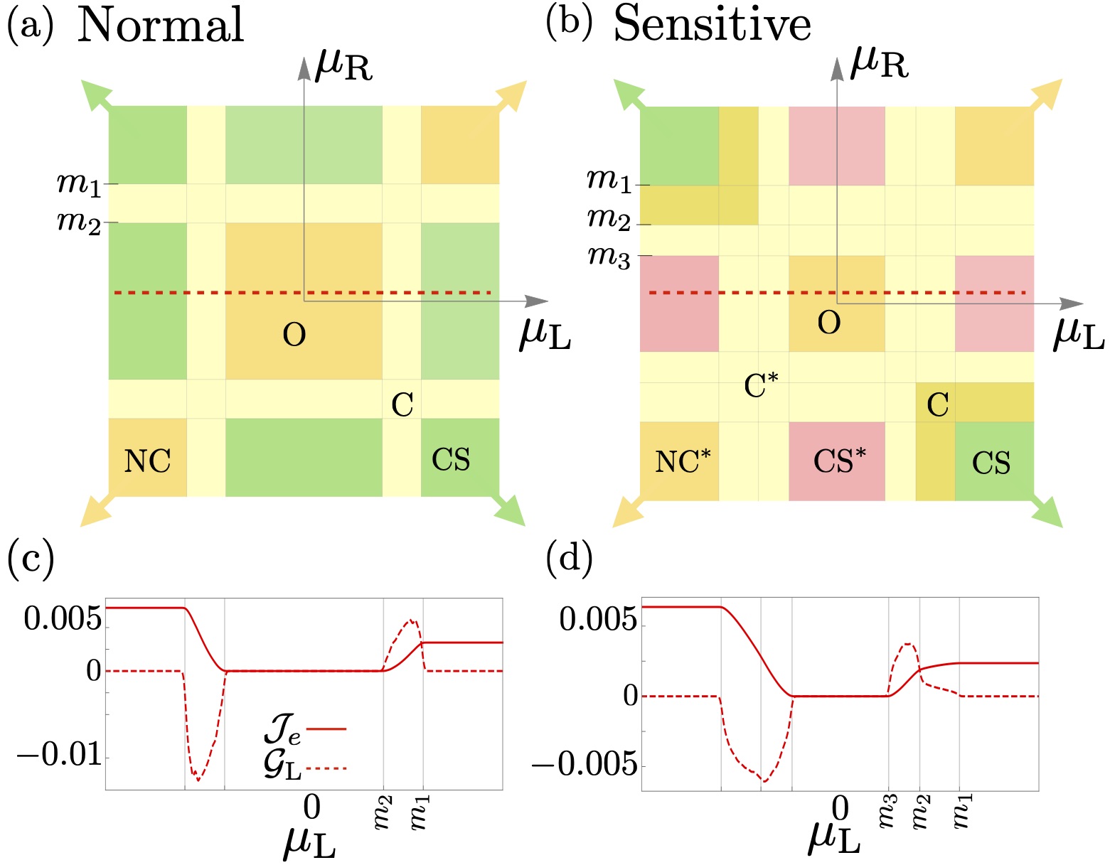
Figure 4: Non-Markovian phase diagram $\mu_{L}\times\mu_{R}$ of two illustrative settings inside the (a) normal and (b) sensitive regions, following the same set of parameters in Fig. 3. The phases were defined as ordered (O), conducting (C), conducting saturated (CS), and non-conducting (NC). In the sensitive case, the phases which acquire a noise in the occupation number are signed with a star ^∗. The arrows at the corners indicate the Markovian limit, i.e. $\left|\mu_{\text{R}}\right|$ and $\left|\mu_{\text{L}}\right|\rightarrow\pm\infty$. (c) and (d) show the current of energy ($\mathcal{J}_{e}$) and the conductance (${\cal G}_{\text{L}}\equiv\partial_{\mu_{\text{L}}}\mathcal{J}_{e}$) computed across the red-dotted lines drawn on the phase diagrams (a) and (b), respectively.

III.4 Occupation numbers

In the current carrying steady-state regime of a Fermi gas, fluctuations in the number of particles were shown to be intimately related to the entanglement entropy of a subsystem (Klich and Levitov, 2009; Song et al., 2010, 2011, 2012). In analogy, the occupation number of the Bogoliubov excitations, given by Eq.(20), can be used to describe the properties of the asymptotic steady-state away from the boundaries. In the open system setting, $n_{k}$ can be approximated by numerically computing the Fourier transform $\boldsymbol{\chi}_{k}=\sum_{r\in\Omega}e^{-ik(r-r_{0})}\boldsymbol{\chi}_{r,r_{0}}$, where $\Omega=\left\{r:L/4<r<3L/4\right\}$ and $r_{0}=L/2$, followed by a Bogoliubov transformation. In equilibrium, $\mu_{L}=\mu_{R}=0$, $n_{k}\simeq 0$ as expected, while in a generic out-of-equilibrium situation $n_{k}\neq 0$.

For the Ising model, it was shown that in the CS and NC phases the $n_{k}$ is a continuous function of $k$, while in the C phase it has discontinuities depending on the reservoir’s chemical potentials (Puel et al., 2019). These discontinuities happen at the momenta $\pm k_{l=\text{L,R}}$ where the chemical potential $\mu_{l=\text{L,R}}$ cross the dispersion relation, see Fig. 5(a). These results extent straightforwardly to the XY-model in the normal region, see Fig. 5(c)-(f). Within the O phase the system behaves as in equilibrium, i.e. $n_{k}\simeq 0$.

In the sensitive region there may be two absolute values of momenta, labelled $\pm k_{l=\text{L,R}}$ and $\pm k^{\prime}_{l=\text{L,R}}$, for which each chemical potential crosses the dispersion relation, as illustrated in Fig. 5(b). Interestingly, we find that $n_{k}$ has an intrinsic noise in the sensitive region, see Figs. 5(g)-(j). The noise appears in phases NC^∗, C^∗, and CS^∗, for $\left|k\right|>k_{m_{2}}$, where $\varepsilon_{k_{m_{2}}}=m_{2}$ (see Fig. 3(c)). In Appendix B we check that the magnitude of the noise in $n_{k}$ does not diminishes with increasing system sizes. Curiously, the noise vanishes along the line $\mu_{\text{L}}=-\mu_{\text{R}}$, as well as within phases C and CS crossed by this line, as shown in Figs. 5(k) and (l), and studied in detail in Appendix B.

Note that $n_{k}$ is asymmetric upon changing $k\to-k$ for all conducting phases as required to maintain a net energy flow through the chain, as $\varepsilon(k)=\varepsilon(-k)$. Figs. 5(c)-5(l) illustrates this feature by showing a larger value of the hybridization, that yield a larger current of energy and consequently to a more asymmetric $n_{k}$.

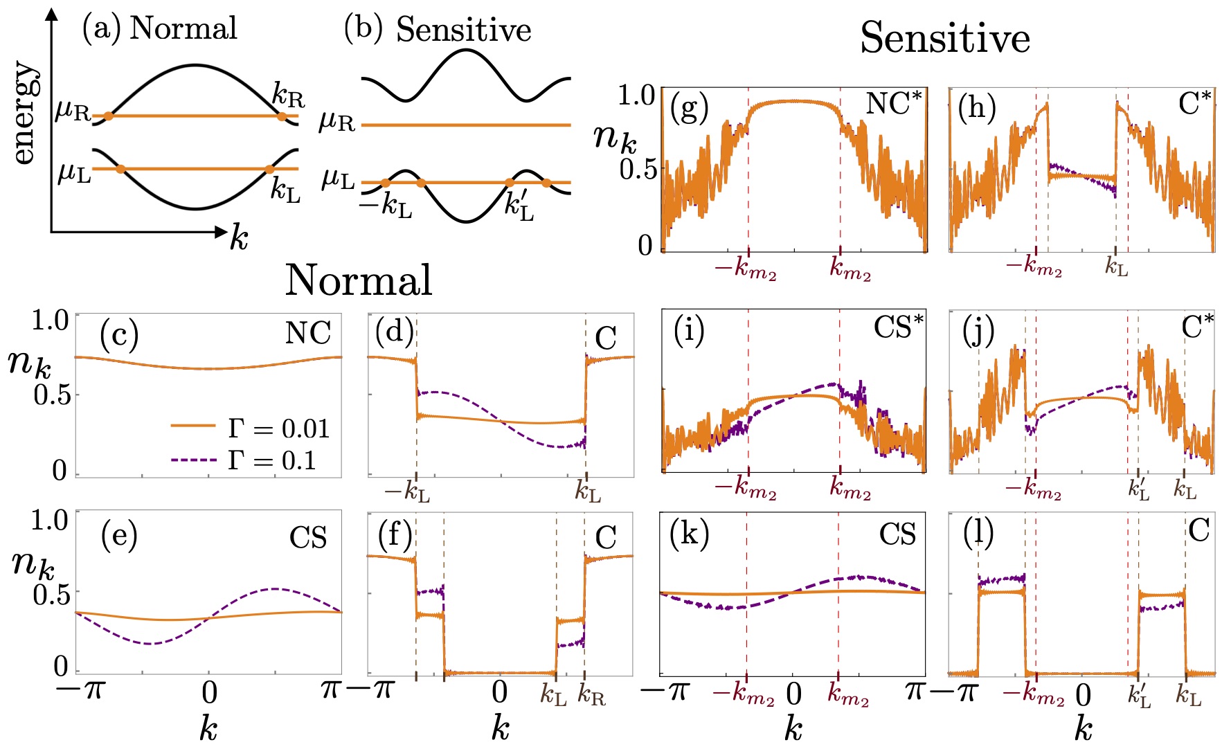
Figure 5: Distribution of occupations. (a) and (b) indicate the momenta $k_{l=\text{L,R}}$ at which the reservoir’s chemical potentials $\mu_{l=\text{L,R}}$ cross the dispersion relation. (c)-(f) illustrate the excitation number $n_{k}$ at different phases inside the normal region. (g)-(l) shows $n_{k}$ in the sensitive region. $k_{m_{2}}$ is such that $\varepsilon_{k_{m_{2}}}=m_{2}$, with $m_{2}$ given in Fig. 3(c).

IV Correlation functions

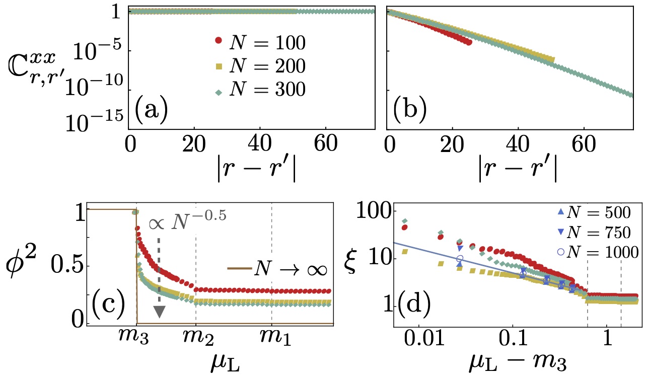
Figure 6: (a) and (b) illustrate the correlation $\mathbb{C}_{r,r^{\prime}}^{xx}$ behavior in the nonequilibrium phases of Fig. 4(b), with fixed $\mu_{\text{R}}=0$. Long-range order only appears in the ordered phase (O), as exemplified in panel (a) at the point $|\mu_{\text{L}}|=0.3<m_{3}$, while a typical exponential decay appears in all other phases, as exemplified in panel (b) for the C^∗ phase at $m_{3}<|\mu_{\text{L}}|=1.3<m_{2}$. (c) and (d) illustrate the mixed-order behavior with a discontinuous order parameter $\phi$ and diverging correlation length $\xi$, respectively, in the thermodynamic limit. The straight line in (d) is a guide to the critical exponent $\nu=1/2$. All panels share the same legends as in (a).

We now consider in more detail the properties of the spin correlation functions, defined in Eq. (21). For $\mathbb{C}_{r,r^{\prime}}^{xx}$, the generic asympototic dependence was already given in Eq. (20) and is able to signal the presence of long-range order when $\phi\neq 0$. We give in Fig. 6(a) a numerical example of this case. On the other hand, when $\phi=0$ we can extract the correlation length $\xi$ from the exponential decay of $\mathbb{C}_{r,r^{\prime}}^{xx}$, see Fig. 6(b). Table 1 shows a summary of the asymptotic dependence of $\mathbb{C}_{r,r^{\prime}}^{xx}$ in the different phases.

Phase	$\mathbb{C}_{r,r^{\prime}}^{xx}\left(\gamma>0\right)$	$\mathbb{C}_{r,r^{\prime}}^{zz}$
O	LRO	EXP
C/C∗	EXP	PL/PL
CS/CS∗	EXP	EXP/PL
NC/NC∗	EXP	EXP/PL

Table 1: Classification of each phase according to the asymptotic behavior of the correlation functions; the possibilities are exponential (EXP) or power law (PL) decay, and long-range order (LRO).

The typical dependence of $\phi$ and $\xi$ on the chemical potential of the reservoirs is illustrated in panels (c) and (d) of Fig. 6, showing the remarkable property of a discontinuity in $\phi$ at the critical point (after extrapolation to the thermodynamic limit) accompanied by a diverging correlation length $\xi$. Further below we will elaborate on the mixed-order transition in more detail, by also providing an analytical description clarifying its origin.

As shown in Table 1, the behavior of $\mathbb{C}_{r,r^{\prime}}^{xx}$ is not affected by the transition to the sensitive region. However, earlier studies showed how, in the Markovian limit, the CS and NC phases are characterized by a transition, from short- to long-range correlations, when entering the sensitive region. This behavior is reflected by a transition from exponential to power-law decay in $\mathbb{C}_{r,r^{\prime}}^{zz}$ Prosen and Pižorn (2008); Žunkovič and Prosen (2010). We observe similar results in the present case, with both non-conducting and saturated phases (CS and NC) showing exponentially-decaying correlations in the normal region and power-law decay in the sensitive one (CS^∗ and NC^∗). Extending the analysis to the highly non-Markovian setting, we find that long-range correlations also appear in the conducting phase, with a power-law decay in both normal (C) and sensitive (C^∗) regions, see Figs. 7(c) and 7(d). These results show that all phases with a noisy excitation number distribution possess power-law decaying $zz$ correlations. The asymptotic behavior of $\mathbb{C}_{r,r^{\prime}}^{zz}$ in the various phases is summarized in Table 1.

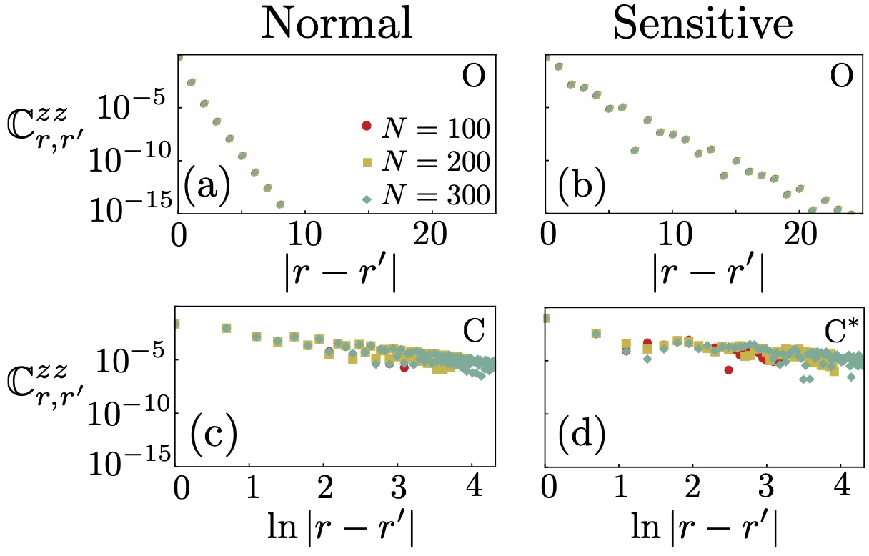
Figure 7: Correlations $\mathbb{C}_{r,r^{\prime}}^{zz}$ for the normal (left column) and sensitive (right column) regions, see Fig. 4. We have set (a) and (b) at $\mu_{\text{L}}=\mu_{\text{R}}=0$, (c) at $m_{2}<|\{\mu_{\text{L}},\mu_{\text{R}}\}=\{2.1,-2.1\}|<m_{1}$, and (d) at $m_{3}<|\{\mu_{\text{L}},\mu_{\text{R}}\}=\{1.3,-1.3\}|<m_{2}$. These results are summarized in Table 1. All panels share the same legends as in (a).

IV.1 Mixed-order phase transition

As aforementioned, for $\gamma>1$, the magnetization along the $x$ direction, $\phi$, is a good order parameter for the broken-symmetry equilibrium phase. In the open system $\phi$ can still be used as order parameter. However, by changing the chemical potential of the, say, left reservoir, $\phi$ drops to zero discontinuously as soon as the system reaches the disordered phase. Interestingly, this transition shows a mixed-order behavior where the discontinuity of $\phi$ is accompanied by a divergence of the correlation length (Puel et al., 2019). The divergence occurs as $\xi\propto\left|\mu_{\text{L}}\pm m_{i}\right|^{-\nu}$ when approaching the critical point from the disordered phase ($i=2,3$ depending on the values of $\gamma$ and $h$). The critical exponent is $\nu=1/2$, except for special values of the parameters (see Appendix C).

We have numerically verified that this behavior survives away from $\gamma=1$, with the same type of dependence of the order parameter and correlation length. In particular, the mixed-order transition with $\nu=1/2$ is also present in the sensitive region, e.g., at the transitions between O and C^∗ phases in the phase diagram of Fig. 4(b). We show in panels (c) and (d) of Fig. 6 an example of the numerical analysis of order parameter and correlation length in the sensitive region. The main difference compared to the normal region is that here finite size effects are much stronger, which is consistent with the sensitive dependence on $N$ of the the rapidity spectrum and occupation numbers, see Figs. 3 and 5.

To derive the value of the critical exponent $\nu$, we consider the explicit form of the correlation function in terms of a Toepliz determinant:(Lieb et al., 1961b; Sachdev, 1996)

$$\left\langle\sigma_{r}^{x}\sigma_{r+n}^{x}\right\rangle=\left|\begin{array}[]{ccccc}D_{0}&D_{-1}&.&.&D_{-n+1}\\ D_{1}&D_{0}&.&.&.\\ .&.&.&.&.\\ .&.&.&D_{0}&D_{-1}\\ D_{n-1}&.&.&D_{1}&D_{0}\end{array}\right|,$$ (24)

where $D_{n}$ is given by:

$$D_{n}=\int\frac{dk}{2\pi}e^{-ink}\sqrt{\frac{1-\left(h/J\right)e^{ik}}{1-\left(h/J\right)e^{-ik}}}\left(1-n_{k}-n_{-k}\right).$$ (25)

The asymptotic dependence can be obtained from Szego’s lemma, leading to the following expression for the correlation length:

$$\xi^{-1}=-\frac{1}{2\pi}\int_{0}^{2\pi}\log\left[1-n_{k}-n_{-k}\right]dk.$$ (26)

Here, the difference from the standard treatment of the transverse-field Ising chain(Lieb et al., 1961b; Sachdev, 1996) is simply that the occupation numbers $n_{k}$ are kept generic, thus are allowed to assume any non-equilibrium distribution induced by the external reservoirs. For example, Eq. (26) takes into account that in general $n_{k}\neq n_{-k}$, as shown by Fig. 5 with a large hybridization energy. By substituting the Fermi distribution, Eqs. (25) and (26) recover the known equilibrium expressions at finite temperature.Sachdev (1996, 2011)

Applying Eq. (26) to the critical point, we first assume as in Fig. 5(a) that the minimum of the quasiparticle dispersion occurs at $k=\pi$. Furthermore, if $\mu_{\rm R}$ is inside the gap the critical point is at $\mu_{\rm L}=m_{2}$. Close to the critical point, the only occupied states are in a small range $k\in[\pi-\Delta k_{\rm L},\pi+\Delta k_{\rm L}]$ around the minimum of $\varepsilon_{k}$, thus we can approximate the quasiparticle dispersion as parabolic giving $\Delta k_{L}\propto\sqrt{\mu_{\rm L}-m_{2}}$. This dependence of $\Delta k_{L}$ is directly related to the critical exponent $\nu=1/2$. More precisely, $\Delta k_{L}$ close to the critical point is given by:

$$\Delta k_{\rm L}\simeq\sqrt{\frac{|1+h/J|}{\gamma^{2}-h/J-1}(\mu_{\rm L}-m_{2})},$$ (27)

and we can set $n_{k}\simeq n_{k=\pi}$ in the small integration interval of Eq. (26), leading to:

$$\xi^{-1}\simeq-\frac{\Delta k_{\rm L}}{\pi}\log\left[1-2n_{\pi}\right].$$ (28)

This expression clearly shows how the divergence of $\xi$ is due to the shrinking of the region of nonzero occupation. We show in Fig. 8 that this theory is accurate, by a direct comparison to the numerical results.

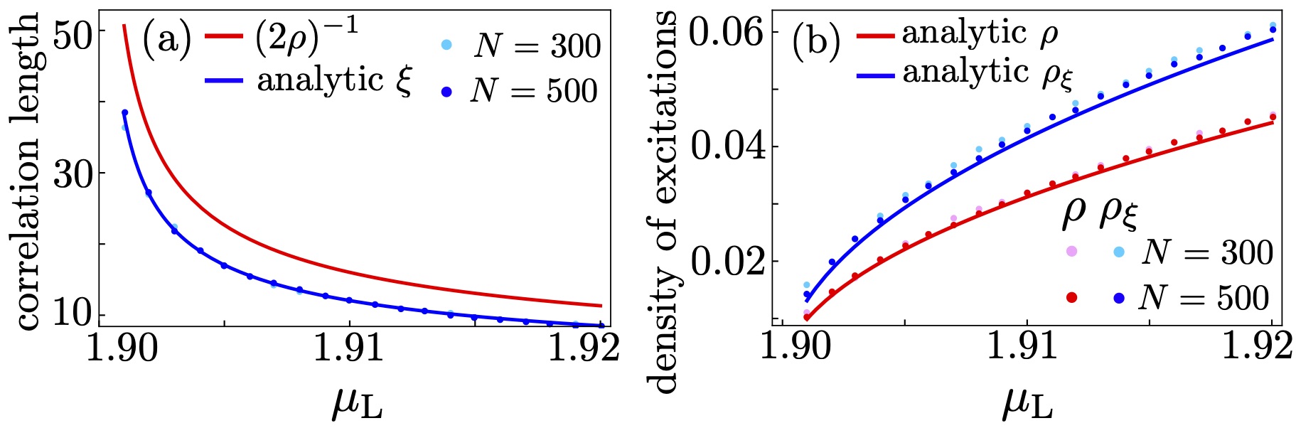
Figure 8: (a): The correlation length of the Ising model ($\gamma=1$), computed at weak transverse field ($h/J=-0.05$) and approaching the critical point $m_{1}=1.9$ from the disordered phase, with $\mu_{\text{R}}=0$. The numerical results (dots) agree well with the blue (lower) curve, given by Eq. (28). The red (upper) curve is from the equilibrium relation $\xi^{-1}=2\rho$, where $\rho=\int_{0}^{2\pi}\frac{dk}{2\pi}n_{k}$ is the density of excitations. (b) Comparison between the numerically computed $\rho$ (upper dots) and the modified density $\rho_{\xi}$ (lower dots), defined in Eq. (30). The solid curves were obtained by assuming a parabolic dispersion and $n_{k}\simeq n_{\pi}$ within the occupied region.

After having clarified the origin of the critical exponent $\nu=1/2$, it is interesting to compare the behavior of the open chain to the temperature dependence of the equilibrium system. In the latter case, an ordered phase is only allowed at zero temperature and the order disappears at any arbitrarily small temperature $T>0$. The sudden disappearance of the ordered state is related to the presence of thermal excitations, and is analogous to the vanishing of $\phi$ induced by the non-equilibrium chemical potentials, as soon as either $\mu_{\rm L}$ or $\mu_{\rm R}$ overcomes the gap. Furthermore, similarly to the non-equilibrium system, the correlation length diverges when $T\to 0$. As it turns out, in the low-temperature limit, $\xi$ can be related in a simple way to the density of excitations $\rho=\int_{0}^{2\pi}\frac{dk}{2\pi}n_{k}$:

$$\xi^{-1}=2\rho.\qquad{\rm(low\mathrm{-}temperature)}$$ (29)

This expression follows immediately from Eq. (26), since $n_{k}=n_{-k}\ll 1$ when $T\to 0$, and can also be understood by a simple argument in terms of a dilute gas of domain-wall excitations.Sachdev (2011)

A naive application of Eq. (29) to the non-equilibrium system is shown in Fig. 8. Although Eq. (29) predicts the correct critical exponent $\nu=1/2$, there is a clear disagreement with the numerical results. This failure of Eq. (29) can be explained from the non-vanishing value of $n_{k}$ around the minimum of $\varepsilon_{k}$ (say, $k=\pi$): in both the low-temperature limit and the non-equilibrium system we have $\rho\to 0$ at the critical point, which results in a diverging correlation length. However, in the first case we have $n_{k}\to 0$ while for the non-equilibrium system $n_{\pi}$ remains finite, and the vanishing of $\rho$ is due to the shrinking of $\Delta k_{L}$. Instead of the density $\rho$, we can consider a ‘modified’ density:

$$\rho_{\xi}=-\frac{1}{4\pi}\int_{0}^{2\pi}\log\left[1-n_{k}-n_{-k}\right]dk,$$ (30)

which follows naturally from Eq. (26) by requiring that a relation similar to the equilibrium system at low temperature is satisfied, $\xi^{-1}=2\rho_{\xi}$. It is easy to see that close the critical point we have $\rho_{\xi}\simeq-(\log\left[1-2n_{\pi}\right]/2n_{\pi})\rho$, which differs from $\rho$ by a nontrivial multiplicative factor. An interesting exception, discussed more extensively in Appendix C, occurs for $J=h/2$, when $n_{\pi}=0$ and the relation between $\xi$ and $\rho$ is Eq. (29), as in equilibrium. At $J=h/2$ the vanishing of $n_{k}$ also affects the value of the critical exponent, which is $\nu=5/2$ instead of 1/2.

The above arguments can be adapted to other parameter regimes. In particular, the discussion is almost unchanged for $h/J<\min[0,\gamma^{2}-1]$, when the dispersion minimum is at $k=0$. Instead, the treatment of the sensitive phase with $|\gamma|<1$ is more delicate. Firstly, as shown in Fig. 5(b), the dispersion is characterized by two minima instead of one. More importantly, $n_{k}$ appears to be highly pathological when $N\to\infty$, when the occupation numbers undergo wild oscillations. Despite these differences, numerical evaluation of the critical exponent still gives $\nu=1/2$, thus we conjecture that a suitable average of $n_{k}$ is well-defined:

$$\overline{n_{k}}=\lim_{\Delta k\to 0}\lim_{N\to\infty}\frac{1}{\Delta k}\int_{k-\frac{\Delta k}{2}}^{k+\frac{\Delta k}{2}}n_{k^{\prime}}dk^{\prime}.$$ (31)

Then, the critical exponent would be determined through Eq. (28) in a way analogous to the regular case, i.e., the critical exponent would correspond to the shrinking of the occupied regions around the minima, explaining the persistence of $\nu=1/2$ in this phase.

IV.2 z-correlations

As summarized in Table 1, $\mathbb{C}_{r,r^{\prime}}^{zz}$ displays a power-law decay in several of the allowed phases. We focus here on the the non-sensitive region, where this behavior can be understood from the well-known power-law decay of density-density correlations of non-interacting fermions. In fact, through the fermionic mapping, $\mathbb{C}_{r,r^{\prime}}^{zz}$ is equivalent to a density-density correlation function:

$$\mathbb{C}_{r,r^{\prime}}^{zz}=4\left(\langle\hat{c}_{r}^{\dagger}\hat{c}_{r}\hat{c}_{r^{\prime}}^{\dagger}\hat{c}_{r^{\prime}}\rangle-\langle\hat{c}_{r}^{\dagger}\hat{c}_{r}\rangle\langle\hat{c}_{r^{\prime}}^{\dagger}\hat{c}_{r^{\prime}}\rangle\right).$$ (32)

In the C phase, at least one of the reservoirs has its chemical potential within the range of quasiparticle energy spectrum. Then, the correlation function is expected to have a power-lay decay with oscillating character, similar to a simple 1D Fermi gas where it decays as $|r-r^{\prime}|^{-2}$ and oscillates with wavevector $2k_{F}$, with $k_{F}$ the Fermi wavevector (see, e.g., Ref. Castin, 2007).

In our case, we express the correlation function through the Bogolubov excitations $\hat{\gamma}_{k}$ of the transnational invariant system (which is appropriate in the thermodynamic limit). The corresponding occupation numbers are defined in Eq. (20) and give:

$$\mathbb{C}_{r,0}^{zz}=\left|\int_{-\pi}^{\pi}\frac{dk}{2\pi}e^{ikr}\left(n_{-k}+n_{k}-1\right)\sin 2\theta_{k}\right|^{2}$$

$$-\left|\int_{-\pi}^{\pi}\frac{dk}{2\pi}e^{ikr}\left[\left(n_{k}+n_{-k}-1\right)\cos 2\theta_{k}+\left(n_{k}-n_{-k}\right)\right]\right|^{2}.$$ (33)

If for simplicity we assume $n_{k}\simeq n_{-k}$ (which is justified in the limit of vanishing hybridization energy $\Gamma$) the occupation numbers have discontinuities at $k=\pm k_{i}$, induced by the left and right reservoirs ($i=L,R$). When $k_{i}r\gg 1$, we can extract the leading contribution to Eq. (IV.2)induced by the discontinuous jumps $\Delta n_{k_{i}}$ of $n_{k}$, defined by $\partial_{k}n_{k}=\sum_{i=L,R}\Delta n_{k_{i}}\left[\delta(k+k_{i})-\delta(k-k_{i})\right]$:

$$\mathbb{C}_{r,0}^{zz}\simeq\frac{4}{\pi^{2}r^{2}} \Bigg{[}\bigg{(}\sum_{i=L,R}\Delta n_{k_{i}}\sin 2\theta_{k_{i}}\cos k_{i}r\bigg{)}^{2}$$

$$- \bigg{(}\sum_{i=L,R}\Delta n_{k_{i}}\cos 2\theta_{k_{i}}\sin k_{i}r\bigg{)}^{2}\Bigg{]},$$ (34)

which simplifies to:

$$\mathbb{C}_{r,0}^{zz}\simeq\frac{4\Delta n_{k_{R}}^{2}}{\pi^{2}r^{2}}\left(\cos^{2}k_{R}r-\cos^{2}2\theta_{k_{R}}\right),$$ (35)

when there is a single Fermi surface (here, induced by $i=R$). The above expressions display the expected $1/r^{2}$ decay and oscillatory dependence. As shown in Fig. 9, we find a good agreement between Eq. (35) and the numerical results.

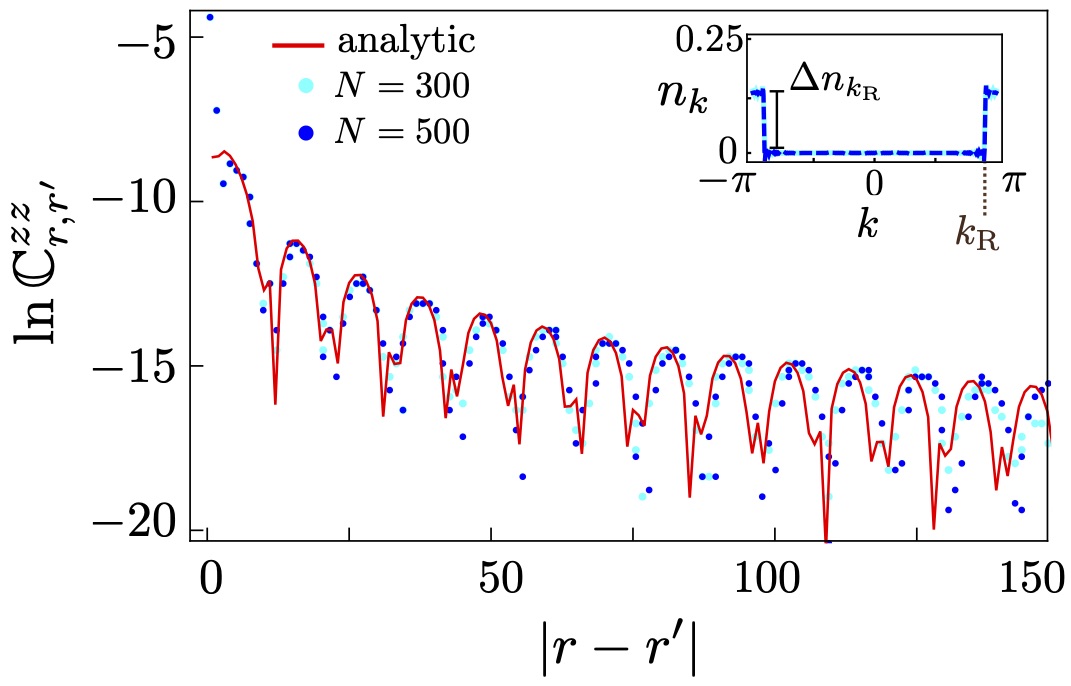
Figure 9: Comparison between numerical results for $\mathbb{C}_{r,r^{\prime}}^{zz}$ (dots) and the analytic approximation Eq. (35) (red curve). The values $\Delta n_{k_{\text{R}}}\simeq 0.1$ and $k_{\text{R}}\simeq 2.85$ were extracted numerically from $n_{k}$, shown in the inset. We used $h=0.2$, $\gamma=1$, $\mu_{\text{L}}=0.5<m_{2}$, and $\mu_{\text{R}}=1.62\gtrsim m_{3}$.

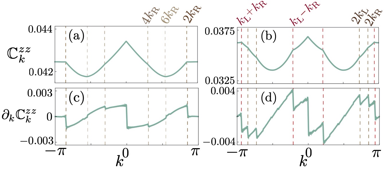
Figure 10: Within the phase diagram of Fig. 4(a), panels (a) and (b) show the Fourier transform of $\mathbb{C}_{r,r^{\prime}}^{zz}$ [see Eq. (36)] for points inside the C phase, namely (a) at $\{\mu_{\text{L}},\mu_{\text{R}}\}=\{-2.9,-2.1\}$ and (b) at $\{\mu_{\text{L}},\mu_{\text{R}}\}=\{-1.9,-2.1\}$. (c) and (d) show their respective derivatives. In the left column we considered the case with only nonzero $k_{\text{R}}$, while the right column considers nonzero $k_{\text{L}}$ and $k_{\text{R}}$. We have computed these results for a system size of $N=500$ sites.

To better characterize the oscillatory dependence, we have also studied the Fourier transform:

$$\mathbb{C}_{k}^{zz}\equiv\frac{1}{\sqrt{N}}\sum_{r-r^{\prime}}\text{e}^{-ik\left(r-r^{\prime}\right)}\mathbb{C}_{r,r^{\prime}}^{zz},$$ (36)

which is shown in Fig. 10 for two representative cases. With a single Fermi surface (left panels) we find dominant non-analytic features at $k=0,2k_{R}$, in agreement with Eq. (35). We also find smaller discontinuities in $\partial_{k}\mathbb{C}_{k}^{zz}$ at higher harmonics, $k=4k_{R},6k_{R}$, which are not captured by the leading-order approximation Eq. (35). With two Fermi surfaces (right panels) we find the expected singularities at $k=0,2k_{L,R}$. However, there are additional features at $\partial_{k}\mathbb{C}_{k}^{zz}$ at $k=k_{L}\pm k_{R}$, which are in agreement with Eq. (IV.2). As seen there, the correlation function is not simply a sum of $i=L,R$ contributions, but involves interference terms between the two Fermi surfaces.

Finally, we comment on the power-law dependence of $\mathbb{C}_{r,r^{\prime}}^{zz}$ in the sensitive region. Away from the ordered phase we find a power-law decay $|r-r^{\prime}|^{-s}$ where, however, the exponent is generally different from $s=2$ (we often find $s<2$) and depends on system parameters. This behavior is most likely related to the singular nature of $n_{k}$, which from our numerical evidence is characterized by a complex pattern of closely spaced discontinuities (see, e.g., Fig. 5). Such discontinuities will contribute to the square parenthesis of Eq. (IV.2) in a way difficult to compute explicitly (the summation index $i$ should become a continuous parameter) and might be able to modify the exponent $s$. This interpretation is confirmed by the survival of the power-lay decay in the NC^∗ and CS^∗ regions, where the chemical potentials $\mu_{\rm L,R}$ do not cross the quasiparticle bands, thus an exponential decay might be expected. Instead, Fig. 5(g) and (i) show that a discontinuous dependence of $n_{k}$ can be found in these regions as well, in agreement with the observed power-law dependence of $\mathbb{C}_{r,r^{\prime}}^{zz}$. Finally, the simple discontinuities of Fig. 5(l) result in the regular value $s=2$.

V Entanglement entropy

In this section, we study the entropy of the steady-state within the different phases identified above. For a segment of $\ell$ sites in the middle of the chain, the entropy is given by

$$E_{\ell}=-\text{Tr}\left[\hat{\rho}_{\ell}\ln\left(\hat{\rho}_{\ell}\right)\right]=-\text{tr}\left[\chi_{\ell}\ln\chi_{\ell}\right],$$ (37)

where $\hat{\rho}_{\ell}$ is the reduced density matrix and $\chi_{\ell}$ is the single-particle correlation matrix restricted to the subsystem of $\ell$ sites. While, for the fermionic system the second equality follows from the non-interacting nature of the problem, this expression was also shown to hold for the spin chain Vidal et al. (2003). In the thermodynamic limit ($N\rightarrow\infty$) the entropy of segment of a translational invariant system is expected to obey the general scaling law(Its and Korepin, 2009)

$$E_{\ell}=l_{0}\ell+c_{0}\ln\left(\ell\right)+c_{1},$$ (38)

where $l_{0}$, $c_{0}$ and $c_{1}$ are $\ell$-independent real constants. For the ground-state of gapped systems $l_{0}=c_{0}=0$ - following the so-called area law, while gapless fermions and spin chains show an universal logarithmic behavior with $c_{0}=1/3$. This result is a consequence of the violation of the area law in $1$+$1$ conformal theories, in which case $c_{0}=c/3$, where $c$ is the central charge(Vidal et al., 2003; Calabrese and Cardy, 2004). For a nonequilibrium Fermi-gas, it was shown that both $l_{0}$ and $c_{0}$ can be non-zero(Eisler and Zimborás, 2014; Ribeiro, 2017), and that $c_{0}$ depends on the system-reservoir coupling and is a non-analytic function of the bias(Ribeiro, 2017). The coefficient $c_{0}$ is most easily extracted from the mutual information, ${\cal I}\left(A,B\right)\equiv E\left(\hat{\rho}_{A}\right)+E\left(\hat{\rho}_{B}\right)-E\left(\hat{\rho}_{A+B}\right)$, of two adjacent segments $A$ and $B$ of size $\ell/2$, since

$${\cal I}_{\ell}\simeq c_{0}\ln\left(\ell\right)+c_{2}.$$ (39)

For the transverse-field Ising model, in Fig. 4(a), all phases, except O, have been shown to have extensive entropy (i.e. $l_{0}\neq 0$) (Puel et al., 2019). This is due to the presence of a finite fraction of excitations, which are absent in the ordered phase. In addition, it was found that $c_{0}\neq 0$ in the C phase, due to the presence of discontinuities in $n_{k}$.

In Fig.11 we show the generalization of the previous results to the $XY$-chain and including the sensitive region of the phase diagram. Fig.11 (a) shows that $l_{0}$ for both normal and sensitive regions. In both cases $l_{0}$ follows the expected value (Ribeiro, 2017):

$$l_{0}=\int\frac{dk}{2\pi}-\left[n_{k}\ln n_{k}+(1-n_{k})\ln(1-n_{k})\right].$$ (40)

On the other hand, ${\cal I}_{\ell}$ does differ qualitatively in the normal and sensitive regions. As aforementioned, logarithmic corrections come from discontinuities in $n_{k}$. If $n_{k}$ has no discontinuities such as in the O and saturated normal phases, $c_{0}$ vanishes. Fig.11 (b) depicts $c_{0}$ in the normal region. The right inset shows that the leading term of ${\cal I}_{\ell}$ in Eq.(39) is indeed logarithmic in the large $\ell$ limit. In principle, for conducting non-saturated phases in the normal region, $c_{0}$ can be computed using the Fisher-Hartwing conjecture Its and Korepin (2009).

The presence of noise in $n_{k}$ within the sensitive region changes the previous picture. The right inset of Fig.11 (b) shows that ${\cal I}_{\ell}$ is no longer of the form given in Eq.(39). It is tempting to interpret this result as a collection of discontinuities of $n_{k}$ whose number increases with system size. However, due to the noisy form of $n_{k}$ it is difficult to give a precise meaning to this picture. Moreover, with the system sizes we could attain, it was not possible to determine the functional for of this correction wit $\ell$. Note that, a supra-logarithmic contribution in ${\cal I}_{\ell}$ is always present in the sensitive region even for the CS^∗ and NC^∗ phases.

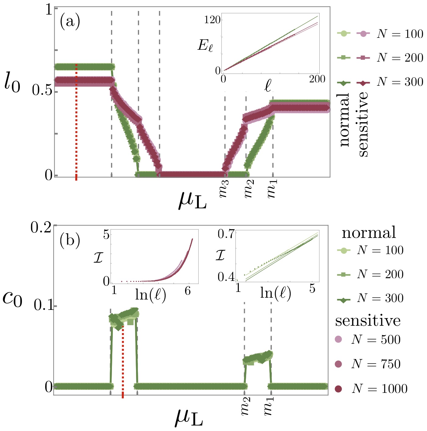
Figure 11: (a) Linear coefficient $l_{0}$, obtained from the entropy scaling law, for a range of $\mu_{\text{L}}$ across the lines depicted in the phase diagrams of Fig. 4. The inset illustrates the typical fitting $E_{\ell}\times\ell$, where the value of $\mu_{\text{L}}$ used is denoted by the dotted-red line. (b) Shows similar results for the logarithmic coefficient $c_{0}$, obtained from Eq.(39), for the same range of $\mu_{\text{L}}$. The inset on the right illustrates the typical fitting ${\cal I}\times\ln\left(\ell\right)$, where the value of $\mu_{\text{L}}$ is denoted by the dotted-red line. In the sensitive region the mutual information is super-logarithmic.

VI Discussions

We have studied the steady-state of a transverse field $XY$-spin chain at zero temperature in a non-equilibrium setting by coupling the ends of the chain to reservoirs which can be held at different magnetic potentials. Our approach is based on a Jordan-Wigner mapping and a Keldysh Green’s function treatment of the resulting non-equilibrium interaction-free fermionic system.

This allows us to study steady-states of the model as a function of the magnetic potentials including the equilibrium and Markovian limits. For magnetic potentials whose magnitudes remain smaller than the spectral gap, the equilibrium-ordered state persists and the correlation function of the order parameter displays long-range order. Away from this phase, the order parameter correlations decay exponentially. As $\mu_{\text{L}}$ or $\mu_{\text{R}}$ reaches the spectral gap, the transition from equilibrium to a current-carrying state occurs through a mixed-ordered transition, where the order parameter vanishes discontinuously while the correlation length diverges. This out-of-equilibrium phenomena was first observed in the Ref. [Puel et al., 2019]. Our present results establish that this behavior is generic to to all order/disorder phase transitions of the $XY$ chain.

For large $\left|\mu_{\text{L}}\right|$ and $\left|\mu_{\text{R}}\right|$ we recover the Markovian limit. We identify the two qualitatively different behaviors previously reported using a Lindblad Master equation approach Prosen and Pižorn (2008); Banchi et al. (2014). We refer to these as (i) sensitive region, featuring algebraic decaying correlations in the transverse (i.e. $z$) direction, and (ii) normal region, where these correlations decay exponentially.

In addition to the equilibrium and Markovian phases, we identify new current-carrying phases. Their properties can be easily understood by studying the quasi-particle excitation number $n_{k}$. By analysing this quantity, we were able to compute the critical exponent of the diverging correlation length at the transition, confirming analytically the results of Ref. [Puel et al., 2019]. The behavior of the transverse correlation function in the normal region is explained in terms of a physical effect which is similar to Friedel oscillations in metals, here observed in a non-equilibrium setting.

For steady-state phases within the sensitive region $n_{k}$ is noisy, for $k$ belonging to the intervals of momentum where the dispersion relation allows four propagating modes. This noise cannot be interpreted as a finite size feature since $n_{k}$, within these regions, does not converge to a thermodynamic limit. Since the transverse correlation function is related to the Fourier transform of $n_{k}$, the pathologies of this function explain the non-exponential decay of transverse correlations in the sensitive region.

We have also analyzed the behavior of the entropy of a segment of the steady-state with its length. As expected for a mixed state, the steady-state entropy is extensive and follows its predicted semi-classical value. In the normal region, whenever the chemical potential lies within one of the bands, there is a logarithmic component that is reminiscent of the area-law violation occurring in equilibrium gapless states. As reported for other non-equilibrium setups Ribeiro (2017), the logarithmic coefficient depends on the discontinuities of $n_{k}$. In the sensitive region, corrections to the extensive contribution turn out to be super-logarithmic.

The analysis presented here generalizes our earlier findings on the transverse field Ising case to the anisotropic XY chain and, thus, extends the class of spin chains which display far-from-equilibrium critical behavior, reflected in a divergent correlation length, that is absent in equilibrium. Thus, the present work suggests that these findings may reflect common features of a wide class of quantum statistical models. A common feature of the models discussed in the present context is their equivalence to interaction-free fermions under a Jordan-Wigner transformation. This naturally poses the question if there exists a finite region in model space around these XY chains where similar non-equilibrium behavior ensures or if their non-thermal behavior is singular. The Jordan-Wigner transformation is limited to one-dimensional systems. Yet, it would be desirable to understand how the non-equilibrium phases that we have identified generalize in higher dimensions.

In equilibrium, interaction-free or quadratic models are commonly associated with fixed point behavior within a field-theoretic description of criticality. This enables one to categorize a wide class of systems into universality classes, with respect to the fixed points. Away from equilibrium, such a categorization is not available. Our results thus offer a vantage point for the construction of a wider class of models that share the same out-of-equilibrium behavior. A better understanding of the universality of far-from-equilibrium critical behavior should prove beneficial for the construction of a field theoretic description of quantum critical matter far from equilibrium.

Appendix A Method detailed

The single-particle density matrix in Eq. (16) is explicitly given by

$$\boldsymbol{\chi}=\frac{1}{2}+\sum_{l=\text{L},\text{R}}\sum_{\alpha\beta}\left|\alpha\right\rangle\left\langle\beta\right|\times\\ \left\langle\tilde{\alpha}\right|\left[\boldsymbol{\gamma}_{l}I_{l}\left(\lambda_{\alpha},\lambda_{\beta}^{*}\right)-\hat{\boldsymbol{\gamma}}_{l}I_{l}\left(-\lambda_{\alpha},-\lambda_{\beta}^{*}\right)\right]\left|\tilde{\beta}\right\rangle$$ (41)

where $I_{l}\left(z,z^{\prime}\right)=-\frac{1}{\pi}\frac{g\left(z-2m_{l}\right)-g\left(z^{\prime}-2m_{l}\right)}{z-z^{\prime}}$ with $g\left(z\right)=\ln\left(-i\text{sgn}\left[\text{Im}\left(z\right)\right]z\right)$, and the matrices $\boldsymbol{\gamma}_{l}$ are defined in Eq. (13). Here we assumed that $\boldsymbol{K}$ in Eq. (13) is diagonalizable, having right and left eigenvectors $\left|\alpha\right\rangle$ and $\left\langle\tilde{\alpha}\right|$ with associated eigenvalues $\lambda_{\alpha}$.

The energy drained to the left reservoir is $\mathcal{J}_{e}=-i\left\langle\left[H,H_{\text{L}}\right]\right\rangle$, which equals the steady-state energy current in any cross section along the chain and thus can be obtained as a function of $\boldsymbol{\chi}$. Explicitly the energy flow can be obtained as $\mathcal{J}_{e}=-\frac{1}{2}\,\text{Tr}\left[\boldsymbol{J}_{r}\boldsymbol{\chi}\right]$ $\forall\,r$, Eq. (23), with

$$\boldsymbol{J}_{r}=-2ihJ\left[(1+{\boldsymbol{S}})\left|r-1\right\rangle\left\langle r\right|(1+{\boldsymbol{S}})-\text{H.c.}\right]\,.$$ (42)

The linear and non-linear thermal conductivities, as well as other thermoelectric properties of the chain, are determined by $\mathcal{J}_{e}$.

A.1 Two-points correlation

Let us further analyse the two-points correlation function in Eq. (21), which can also be found in terms of $\boldsymbol{\chi}$. To this end we have extended the equilibrium expressions(Lieb et al., 1961a) to general non-equilibrium conditions:

$$\mathbb{C}_{r,r^{\prime}}^{xx} = \det\left[i\left(2\boldsymbol{\chi}_{\left[r,r^{\prime}\right]}-1\right)\right]^{\frac{1}{2}}$$ (43)

for $r>r^{\prime}+1$, where $\boldsymbol{\chi}_{\left[r,r^{\prime}\right]}$ is a $2\left(r-r^{\prime}\right)$ matrix obtained as the restriction of $\boldsymbol{\chi}$ to the subspace in which $\mathbb{P}_{rr^{\prime}}^{T}=\sum_{u=r^{\prime}+1}^{r-1}\left(\left|u\right\rangle\left\langle u\right|+\left|\hat{u}\right\rangle\left\langle\hat{u}\right|\right)+\left|r_{+}\right\rangle\left\langle r_{+}\right|+\left|r^{\prime}_{-}\right\rangle\left\langle r^{\prime}_{-}\right|$, with $\left|r_{\pm}\right\rangle=\left(\left|r\right\rangle\pm\left|\hat{r}\right\rangle\right)/\sqrt{2}$, acts as the identity, and $\left|r\right\rangle$ and $\left|\hat{r}\right\rangle\equiv\boldsymbol{S}\left|r\right\rangle$ are single-particle and hole states.

Appendix B Excitation number

The intriguing results of the occupation number, computed in section IIID, deserve a more detail analysis as follows. As discussed in the manuscript, the occupation number shows a noise behavior in some of the phases, thus, in order to give the reader a complete view of the possible cases, in Fig. 13 we show the occupation number for one representative point in each phase, as marked in Fig. 12(a). Here we have set the system in the sensitive region with transverse magnetic field $h/J=0.2$ and anisotropy $\gamma=0.5$. The marks are at the points $\mu_{\text{L}},\mu_{\text{R}}=\{\pm 2.7,\pm 1.9,\pm 1.3,+0.3\text{ or}-0.3\}$.

As discussed in the manuscript, here we clearly see that the noise is present on the phases around the axis $\mu_{\text{L}}=\mu_{\text{R}}$, while it vanishes around the axis $\mu_{\text{L}}=-\mu_{\text{R}}$. The noise only appears for $\left|k\right|>k_{m_{2}}$, see Fig. 3(c). In addition, it is persistent even in the thermodynamic limit, as shows Fig. 12(b).

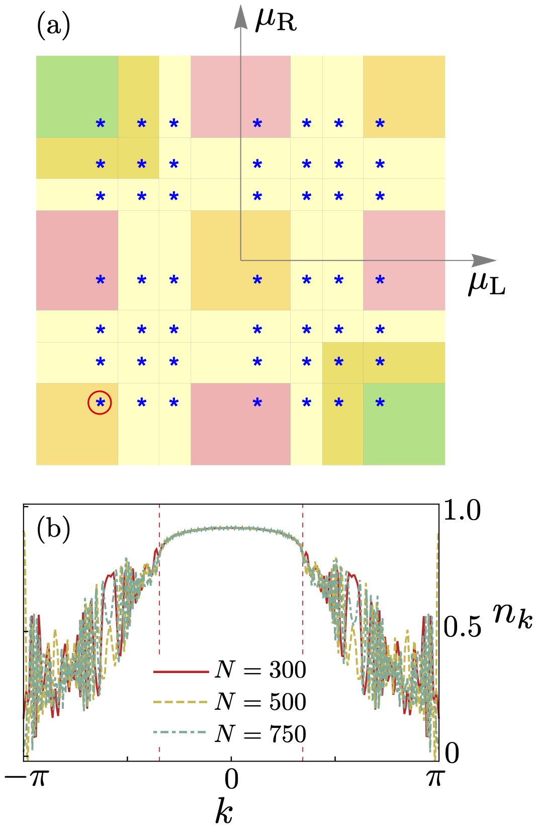
Figure 12: (a) repeats the phase diagram of Fig. 4(b). The blue stars mark the parameters used in Fig. 13. Panel (b) illustrates the persistent noise in the occupation number, computed for different system sizes, with set of parameters indicated by the circled blue star on the phase diagram.

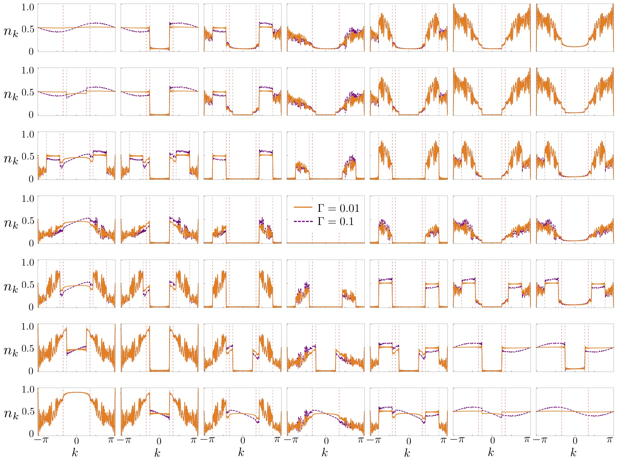
Figure 13: Excitation number $n_{k}$ in the sensitive region for different phases. Each plot represents a different set of parameters $\left\{\mu_{\text{L}},\mu_{\text{R}}\right\}$ marked on the phase diagram in Fig. 12(a) disposed in the same order. We have computed it for a system size of $N=500$ sites. The vertical dashed lines represent either the momentum $k_{m_{2}}$ or $k_{\text{L}}$, see Figs. 3(c) and 5(a) and 5(b).

Appendix C Correlation length at $h/J=0.5$

When $h/J=0.5$, it was observed that $n_{k=\pi}=0$,Puel et al. (2019) thus the derivation of Eq. (28) should be modified. Interestingly, around $k=\pi$ we find that $n_{k}$ has a leading term of the form:

$$n_{k}\simeq c(k-\pi)^{4},$$ (44)

where the vanishing of the quadratic term and the value of $c$ could only be obtained numerically. In the limit of a small $\Delta k_{\rm L}$, Eq. (26) yields:

$$\xi^{-1}\simeq\frac{c}{\pi}\int_{-\Delta k_{\rm L}}^{\Delta k_{\rm L}}x^{4}dx=\frac{2c}{5\pi}\Delta k_{\rm L}^{5}.$$ (45)

Finally, from the expression of $\Delta k_{\rm L}$ in Eq. (27) we immediately see that the critical exponent is $\nu=5/2$. It is also worth mentioning that, since $n_{k}$ becomes vanishingly small approaching the critical point, Eq. (30) coincides with the regular density and the relation $\xi^{-1}=2\rho$ is still valid. Figure 14 shows the comparison of these results with the numerical calculations.

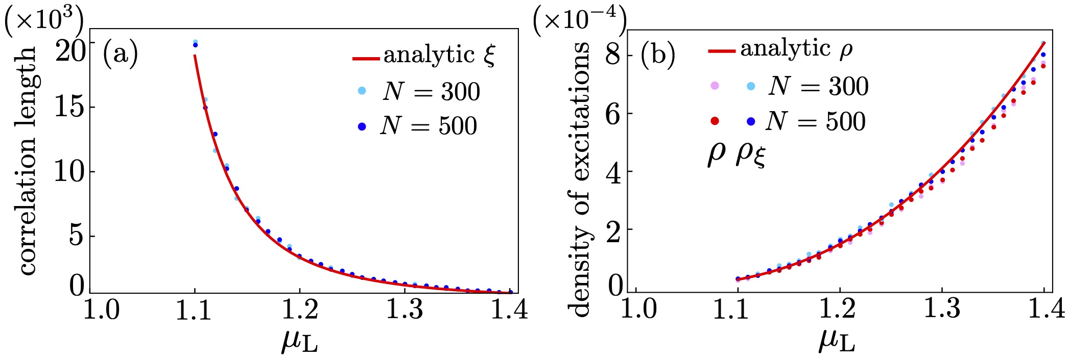
Figure 14: (a) Correlation length of the Ising model ($\gamma=1$) for the special case $h/J=0.5$ and approaching the critical point $m_{2}=1$ from the disordered phase (C), with $\mu_{\text{R}}=0$. The dots and continuous line compare the numerical result, Eq. (22), to the analytic result, Eq. (45), respectively. (b) Density of excitations $\rho$ and $\rho_{\xi}$, given by Eq. (30). The continuous line shows the analytic result for $\rho$, computed from Eq. (45) as $\rho=\xi^{-1}/2$. In the analytic formulas we have used the educated guess $c=\pi/5!$.

References

- Pothier et al. (1997) H. Pothier, S. Guéron, N. O. Birge, D. Esteve, and M. H. Devoret, Phys. Rev. Lett. 79, 3490 (1997).
- Anthore et al. (2003) A. Anthore, F. Pierre, H. Pothier, and D. Esteve, Phys. Rev. Lett. 90, 076806 (2003).
- Chen et al. (2009) Y.-F. Chen, T. Dirks, G. Al-Zoubi, N. O. Birge, and N. Mason, Phys. Rev. Lett. 102, 036804 (2009).
- Brantut et al. (2013) J.-P. Brantut, C. Grenier, J. Meineke, D. Stadler, S. Krinner, C. Kollath, T. Esslinger, and A. Georges, Science 342, 713 (2013).
- Büttiker and Landauer (1982) M. Büttiker and R. Landauer, Phys. Rev. Lett. 49, 1739 (1982).
- Stefanucci and van Leeuwen (2013) G. Stefanucci and R. van Leeuwen, Nonequilibrium Many-Body Theory of Quantum Systems: A Modern Introduction (Cambridge University Press, 2013).
- Datta et al. (1997) S. Datta, H. Ahmad, and M. Pepper, Electronic Transport in Mesoscopic Systems, Cambridge Studies in Semiconductor Physi (Cambridge University Press, 1997).
- Imry (2002) Y. Imry, Introduction to Mesoscopic Physics, Mesoscopic physics and nanotechnology (Oxford University Press, 2002).
- Aoki et al. (2014) H. Aoki, N. Tsuji, M. Eckstein, M. Kollar, T. Oka, and P. Werner, Rev. Mod. Phys. 86, 779 (2014).
- Gutman et al. (2008) D. B. Gutman, Y. Gefen, and A. D. Mirlin, Phys. Rev. Lett. 101, 126802 (2008).
- Gutman et al. (2009) D. B. Gutman, Y. Gefen, and A. D. Mirlin, Phys. Rev. B 80, 045106 (2009).
- Ngo Dinh et al. (2010) S. Ngo Dinh, D. A. Bagrets, and A. D. Mirlin, Phys. Rev. B 81, 081306(R) (2010).
- Prosen and Pižorn (2008) T. Prosen and I. Pižorn, Phys. Rev. Lett. 101, 105701 (2008).
- Prosen and Žunkovič (2010) T. Prosen and B. Žunkovič, New J. Phys. 12, 025016 (2010).
- Prosen (2011) T. Prosen, Phys. Rev. Lett. 107, 137201 (2011).
- Prosen (2014) T. Prosen, Phys. Rev. Lett. 112, 030603 (2014).
- Ribeiro and Vieira (2015a) P. Ribeiro and V. R. Vieira, Phys. Rev. B 92, 100302(R) (2015a), arXiv:1412.8486 .
- Ribeiro and Vieira (2015b) P. Ribeiro and V. R. Vieira, in Symmetry, Spin Dynamics and the Properties of Nanostructures (World Scientific, 2015) pp. 86–111.
- Bertini et al. (2016) B. Bertini, M. Collura, J. De Nardis, and M. Fagotti, Phys. Rev. Lett. 117, 207201 (2016).
- Castro-Alvaredo et al. (2016) O. A. Castro-Alvaredo, B. Doyon, and T. Yoshimura, Phys. Rev. X 6, 041065 (2016).
- Arrigoni et al. (2013) E. Arrigoni, M. Knap, and W. von der Linden, Phys. Rev. Lett. 110, 086403 (2013).
- Puel et al. (2019) T. O. Puel, S. Chesi, S. Kirchner, and P. Ribeiro, Phys. Rev. Lett. 122, 235701 (2019).
- Thouless (1969) D. J. Thouless, Phys. Rev. 187, 732 (1969).
- Bar and Mukamel (2014) A. Bar and D. Mukamel, Phys. Rev. Lett. 112, 015701 (2014).
- Fronczak et al. (2016) A. Fronczak, P. Fronczak, and A. Krawiecki, Phys. Rev. E 93, 012124 (2016).
- Anglès d’Auriac and Iglói (2016) J.-C. Anglès d’Auriac and F. Iglói, Phys. Rev. E 94, 062126 (2016).
- Juhász and Iglói (2017) R. Juhász and F. Iglói, Phys. Rev. E 95, 022109 (2017).
- Alert et al. (2017) R. Alert, P. Tierno, and J. Casademunt, Proceedings of the National Academy of Sciences 114, 12906 (2017).
- Žunkovič and Prosen (2010) B. Žunkovič and T. Prosen, Journal of Statistical Mechanics: Theory and Experiment 2010, P08016 (2010).
- Ajisaka et al. (2014) S. Ajisaka, F. Barra, and B. Žunkovič, New Journal of Physics 16, 033028 (2014).
- Lieb et al. (1961a) E. Lieb, T. Schultz, and D. Mattis, Annals of Physics 16, 407 (1961a).
- Kitaev (2001) A. Y. Kitaev, Phys. Usp. 44, 131 (2001).
- Meier and Loss (2003) F. Meier and D. Loss, Phys. Rev. Lett. 90, 167204 (2003).
- Nakata et al. (2017) K. Nakata, P. Simon, and D. Loss, Journal of Physics D: Applied Physics 50, 114004 (2017).
- Hoffman et al. (2018) S. Hoffman, D. Loss, and Y. Tserkovnyak, “Superfluid transport in quantum spin chains,” (2018), arXiv:1810.11470 [cond-mat.mes-hall] .
- Shen et al. (2020) P.-X. Shen, S. Hoffman, and M. Trif, “Theory of topological spin josephson junction,” (2020), arXiv:1912.11458 [cond-mat.mes-hall] .
- Barouch and McCoy (1971) E. Barouch and B. M. McCoy, Phys. Rev. A 3, 786 (1971).
- Lieb et al. (1961b) E. Lieb, T. Schultz, and D. Mattis, Annals of Physics 16, 407 (1961b).
- Sachdev (1996) S. Sachdev, Nuclear Physics B 464, 576 (1996).
- Banchi et al. (2014) L. Banchi, P. Giorda, and P. Zanardi, Phys. Rev. E 89, 022102 (2014), arXiv:1305.4527 .
- Medvedyeva and Kehrein (2014) M. V. Medvedyeva and S. Kehrein, Phys. Rev. B 90, 1 (2014), arXiv:1406.1408 .
- Klich and Levitov (2009) I. Klich and L. Levitov, Phys. Rev. Lett. 102, 100502 (2009).
- Song et al. (2010) H. F. Song, S. Rachel, and K. Le Hur, Phys. Rev. B 82, 012405 (2010).
- Song et al. (2011) H. F. Song, C. Flindt, S. Rachel, I. Klich, and K. Le Hur, Phys. Rev. B 83, 161408 (2011).
- Song et al. (2012) H. F. Song, S. Rachel, C. Flindt, I. Klich, N. Laflorencie, and K. Le Hur, Phys. Rev. B 85, 035409 (2012).
- Sachdev (2011) S. Sachdev, Quantum Phase Transitions, 2nd ed. (Cambridge University Press, 2011).
- Castin (2007) Y. Castin, in Proceedings of the International School of Physics “Enrico Fermi”, edited by M. Inguscio, W. Ketterle, and C. Salomon (SIF, Bologna, Italy, 2007) pp. 289–349.
- Vidal et al. (2003) G. Vidal, J. I. Latorre, E. Rico, and A. Kitaev, Phys. Rev. Lett. 90, 227902 (2003).
- Its and Korepin (2009) A. R. Its and V. E. Korepin, Journal of Statistical Physics 137, 1014 (2009).
- Calabrese and Cardy (2004) P. Calabrese and J. Cardy, J. Stat. Mech. 2004, P06002 (2004).
- Eisler and Zimborás (2014) V. Eisler and Z. Zimborás, Phys. Rev. A 89, 032321 (2014).
- Ribeiro (2017) P. Ribeiro, Phys. Rev. B 96, 054302 (2017).