Quantum Critical Point between Two-Channel Kondo and Fermi-Liquid Phases

Abstract

We investigate the emergence of quantum critical points near a two-channel Kondo phase by evaluating an $f$-electron entropy of a seven-orbital impurity Anderson model hybridized with three ($\Gamma_{7}$ and $\Gamma_{8}$) conduction bands with the use of a numerical renormalization group method. First we consider the case of Pr³⁺ ion, in which quadrupole two-channel Kondo effect is known to occur for the local $\Gamma_{3}$ doublet state. When we control crystalline electric field (CEF) potentials so as to change the local CEF ground state from $\Gamma_{3}$ doublet to $\Gamma_{1}$ singlet or $\Gamma_{5}$ triplet, we commonly observe a residual entropy of $\log\phi$ with the golden ratio $\phi=(1+\sqrt{5})/2$, which is equal to that for three-channel Kondo effect. This peculiar residual entropy is also observed for the case of Nd³⁺ ion, in which magnetic two-channel Kondo phase is found to occur for the local $\Gamma_{6}$ doublet state. We envisage a scenario that the quantum critical point characterized by $\log\phi$ generally appears between two-channel Kondo and Fermi-liquid phases.

1 Introduction

In the modern condensed matter physics, quantum critical phenomena have attracted continuous attention, since exotic and intriguing electronic phases have incessantly emerged near a quantum critical point (QCP). One of typical phenomena emerging from QCP is a non-Fermi-liquid state. In particular, a stage for the non-Fermi-liquid ground state is provided by two-channel Kondo effect. After the understanding of the conventional Kondo effect,[1] Coqblin and Schrieffer have derived exchange interactions from the multiorbital Anderson model.[2] Then, a concept of multi-channel Kondo effect has been developed on the basis of such exchange interactions,[3] as a potential source of non-Fermi-liquid phenomena.

Concerning the reality of two-channel Kondo effect, Cox has pointed out that it actually occurs in a cubic uranium compound with non-Kramers doublet ground state.[4, 5] Namely, for the $\Gamma_{3}$ ground state, there exist anti-ferro exchange interactions in terms of quadrupole degree of freedom between localized and conduction electrons, whereas spin degree of freedom plays a role of channel. On the other hand, a non-Fermi-liquid state has been pointed out in a two-impurity Kondo system.[6, 7, 8] This phenomenon has attracted much attention from a viewpoint of QCP and it has been confirmed that the QCP appears at the transition between the screened Kondo and local singlet phases. The two-channel Kondo effect and properties of the QCP have been vigorously discussed for a long time by numerous authors. [9, 10, 11, 12, 13, 14, 15, 16, 17, 18, 19, 20, 21, 22, 23, 24, 25, 26, 27, 28, 29, 30]

We believe that the two-channel Kondo effect itself gives an inexhaustible source of non-trivial intriguing phenomena, but here we turn our attention to the QCP near the two-channel Kondo phase. In particular, we are much interested in the emergence of QCP when two $4f$ electrons of Pr³⁺ ion are hybridized with three ($\Gamma_{7}$ and $\Gamma_{8}$) conduction bands. The QCP in the vicinity of quadrupole two-channel Kondo phase is expected to be experimentally observed in Pr compounds, since there recently have been significant advances to grasp the signal of non-Fermi-liquid behavior in Pr compounds. [31]

In this study, we analyze a seven-orbital impurity Anderson model hybridized with $\Gamma_{7}$ and $\Gamma_{8}$ conduction bands by using a numerical renormalization group (NRG) method.[32, 33] For Pr³⁺ ion, by controlling crystalline electric field (CEF) potentials between two-channel Kondo and CEF singlet phases, we find a residual entropy of $\log\phi$ with $\phi=(1+\sqrt{5})/2$, which is the same as that for three-channel Kondo effect. This entropy also appears between two-channel Kondo and screened Kondo singlet phases, and we also find it when the hybridization is increased in the two-channel Kondo phase. Furthermore, when we analyze the model for Nd³⁺ ion to consider magnetic two-channel Kondo phase,[26] we find a $\log\phi$ plateau in the temperature dependence of the entropy. Then, we envisage that in general, the QCP characterized by $\log\phi$ appears between two-channel Kondo and Fermi-liquid phases.

The paper is organized as follows. In Sect. 2, for the description of the local $f$-electron states, first we explain the local Hamiltonian including spin-orbit couping, CEF potentials, and Coulomb interactions among $f$ electrons. After checking the local $f$-electron states for Pr³⁺ and Nd³⁺ ions, we construct an impurity Anderson model by considering the hybridization between localized and conduction electrons in $\Gamma_{8}$ and $\Gamma_{7}$ orbitals. We also explain the NRG method to analyze the impurity Anderson model. In Sect. 3, we review the previous results for the two-band case, in which we have included only the hybridization in the $\Gamma_{8}$ electrons for Pr³⁺ and Nd³⁺ ions. In particular, we explain the two-channel Kondo effect on the basis of a $j$-$j$ coupling scheme. In Sect. 4, we show our NRG results for the case in which we consider the hybridization for $\Gamma_{8}$ and $\Gamma_{7}$ electrons. We remark the emergence of QCP’s between two-channel Kondo and Fermi-liquid phases for Pr³⁺ and Nd³⁺ ions. Finally, in Sect. 5, we provide a few comments on the future problems and a possibility to detect the present QCP in actual materials. Throughout this paper, we use such units as $\hbar=k_{\rm B}=1$.

2 Model and Method

2.1 Local Hamiltonian

Let us start our discussion on the description of the local $f$-electron state. For the purpose, first we consider one $f$-electron state, which is the eigenstate of spin-orbit and CEF terms. Then, we include Coulomb interactions among $f$ electrons. As shown in the left part of Fig. 1, under the cubic CEF potentials, we obtain $\Gamma_{7}$ doublet and $\Gamma_{8}$ quartet from $j=5/2$ sextet, whereas $\Gamma_{6}$ doublet, $\Gamma_{7}$ doublet, and $\Gamma_{8}$ quartet from $j=7/2$ octet. By using those one-electron states as bases, we express the local $f$-electron Hamiltonian as

$$\begin{split}H_{\rm loc}&=\sum_{j,\mu,\tau}(\lambda_{j}+B_{j,\mu})f_{j\mu\tau}^{{\dagger}}f_{j\mu\tau}+nE_{f}\\ &+\sum_{j_{1}\sim j_{4}}\sum_{\mu_{1}\sim\mu_{4}}\sum_{\tau_{1}\sim\tau_{4}}I^{j_{1}j_{2},j_{3}j_{4}}_{\mu_{1}\tau_{1}\mu_{2}\tau_{2},\mu_{3}\tau_{3}\mu_{4}\tau_{4}}\\ &\times f_{j_{1}\mu_{1}\tau_{1}}^{{\dagger}}f_{j_{2}\mu_{2}\tau_{2}}^{{\dagger}}f_{j_{3}\mu_{3}\tau_{3}}f_{j_{4}\mu_{4}\tau_{4}},\end{split}$$ (1)

where $f_{j\mu\tau}$ denotes the annihilation operator of a localized $f$ electron in the bases of $(j,\mu,\tau)$, $j$ is the total angular momentum, $j=5/2$ and $7/2$ are denoted by “$a$” and “$b$”, respectively, $\mu$ distinguishes the cubic irreducible representation, $\Gamma_{8}$ states are distinguished by $\mu=\alpha$ and $\beta$, while $\Gamma_{7}$ and $\Gamma_{6}$ states are labeled by $\mu=\gamma$ and $\delta$, respectively, $\tau$ is the pseudo-spin which distinguishes the degeneracy concerning the time-reversal symmetry, $n$ is the local $f$-electron number at an impurity site, and $E_{f}$ is the $f$-electron level to control $n$. Throughout this paper, the energy unit is set as eV.

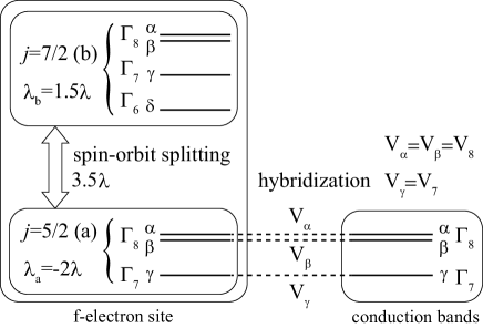
Figure 1: Schematic view of the seven-orbital impurity Anderson model. The left part of this figure denotes the local $f$-electron states described by a $j$-$j$ coupling scheme, in which Coulomb interactions among such states are further included. The lower right part indicates three conduction electron bands, hybridized with the $j=5/2$ states of the same irreducible representations.

As for the spin-orbit term, we obtain

$$\lambda_{a}=-2\lambda,~{}\lambda_{b}=(3/2)\lambda,$$ (2)

where $\lambda$ is the spin-orbit coupling of $f$ electron. In this paper, we set $\lambda=0.1$ and $0.11$ for Pr and Nd ions, respectively. Concerning the CEF potential term for $j=5/2$, we obtain

$$\begin{split}B_{a,\alpha}&=B_{a,\beta}=1320B_{4}^{0}/7,\\ B_{a,\gamma}&=-2640B_{4}^{0}/7,\end{split}$$ (3)

where $B_{4}^{0}$ denotes the fourth-order CEF parameter in the table of Hutchings for the angular momentum $\ell=3$. [34] Note that the sixth-order CEF potential term $B_{6}^{0}$ does not appear for $j=5/2$, since the maximum size of the change of the total angular momentum is less than six in this case. On the other hand, for $j=7/2$, we obtain

$$\begin{split}B_{b,\alpha}&=B_{b,\beta}=360B_{4}^{0}/7+2880B_{6}^{0},\\ B_{b,\gamma}&=-3240B_{4}^{0}/7-2160B_{6}^{0},\\ B_{b,\delta}&=360B_{4}^{0}-3600B_{6}^{0}/7.\end{split}$$ (4)

Note that the $B_{6}^{0}$ terms turn to appear in this case. In the present calculations, we treat $B_{4}^{0}$ and $B_{6}^{0}$ as parameters.

The Coulomb interaction $I$ is expressed as

$$\begin{split}&I^{j_{1}j_{2},j_{3}j_{4}}_{\mu_{1}\tau_{1}\mu_{2}\tau_{2},\mu_{3}\tau_{3}\mu_{4}\tau_{4}}=\sum_{m_{1}\sim m_{4}}\sum_{\sigma,\sigma^{\prime}}C_{j_{1}\mu_{1}\tau_{1},m_{1}\sigma}\\ &\times C_{j_{2}\mu_{2}\tau_{2},m_{2}\sigma^{\prime}}C_{j_{3}\mu_{3}\tau_{3},m_{3}\sigma^{\prime}}C_{j_{4}\mu_{4}\tau_{4},m_{4}\sigma}\\ &\times\sum_{k=0}^{6}F^{k}c_{k}(m_{1},m_{4})c_{k}(m_{2},m_{3}),\end{split}$$ (5)

where $m$ is the $z$ component of the angular momentum $\ell=3$, $\sigma$ denotes a real spin, the sum of $k$ is limited by the Wigner-Eckart theorem to the even numbers, $F^{k}$ indicates the Slater-Condon parameter, $c_{k}$ is the Gaunt coefficient,[35] and $C$ denotes the coefficient in the transformation of

$$f_{j\mu\tau}=\sum_{m,\sigma}C_{j\mu\tau,m\sigma}f_{m\sigma}.$$ (6)

Although the Slater-Condon parameters of the material should be determined from experimental results, here we simply set the ratio as [36]

$$F^{0}/10=F^{2}/5=F^{4}/3=F^{6}=U,$$ (7)

where $U$ is the Hund’s rule interaction among $f$ orbitals. In this study, we set $U$ as 1 eV.

2.2 Local $f$-electron states

First let us consider the local CEF ground-state phase diagram for the case of $n=2$. The ground-state multiplet for $B_{4}^{0}=B_{6}^{0}=0$ is characterized by total angular momentum $J=4$. Under the cubic CEF potentials, the nonet of $J=4$ is split into four groups as $\Gamma_{1}$ singlet, $\Gamma_{3}$ doublet, $\Gamma_{4}$ triplet, and $\Gamma_{5}$ triplet. Among them, $\Gamma_{4}$ triplet does not appear as a solo ground state under the cubic CEF potential with $O_{\rm h}$ symmetry. Then, we obtain three local ground states for $n=2$, as shown in Fig. 2(a).

Roughly speaking, we obtain $\Gamma_{1}$ singlet for $B_{4}^{0}>0$, whereas $\Gamma_{5}$ triplet appears for $B_{4}^{0}<0$. Here we recall the fact that $f^{1}$ local ground state is $\Gamma_{7}$ and $\Gamma_{8}$ for $B_{4}^{0}>0$ and $B_{4}^{0}<0$, respectively. When we accommodate two electrons into these situations, we easily obtain $\Gamma_{1}$ singlet and $\Gamma_{5}$ triplet by standard positive Hund’s rule interaction. As for $\Gamma_{3}$ doublet state, it appears for $B_{6}^{0}>0$ near the region of $B_{4}^{0}\approx 0$. The stabilization of $\Gamma_{3}$ doublet is understood by effective negative Hund’s rule interaction, which depends on $B_{6}^{0}$.[28]

In the following calculations, we use the parametrization as

$$B_{4}^{0}=Wx/F(4),~{}~{}B_{6}^{0}=W(1-|x|)/F(6),$$ (8)

where $x$ specifies the CEF scheme for the $O_{\rm h}$ point group, whereas $W$ determines the energy scale for the CEF potentials.[37] We choose $F(4)=15$ and $F(6)=180$ for $\ell=3$.[34] The trajectory of $B_{4}^{0}$ and $B_{6}^{0}$ for $-1\leq x\leq 1$ with a fixed value of $|W|$ ($W>0$ and $W<0$) forms a rhombus on the $(B_{4}^{0},B_{6}^{0})$ plane. The trajectories for $|W|=0.001$ and $0.002$ are shown in red and blue rhombuses, respectively, in Figs. 2.

In Fig. 2(b), we show the local CEF ground-state phase diagram for the case of $n=3$. The ground-state multiplet for $B_{4}^{0}=B_{6}^{0}=0$ is characterized by $J=9/2$. Under the cubic CEF potentials, the dectet of $J=9/2$ is split into three groups as one $\Gamma_{6}$ doublet and two $\Gamma_{8}$ quartets. Then, we obtain two local ground states for $n=3$, as shown in Fig. 2(b). Note that the $\Gamma_{6}$ doublet appears in the region of $B_{6}^{0}>0$, which is the same side as that of the $\Gamma_{3}$ doublet. When we consider the $f$-electron states on the basis of a $j$-$j$ coupling scheme, the $\Gamma_{6}$ doublet for $n=3$ is obtained by putting one electron to the vacant orbital in the $\Gamma_{3}$ doublet for $n=2$.[26, 38] This point will be discussed later again.

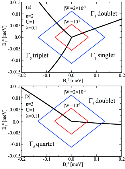
Figure 2: (Color online) Local CEF ground-state phase diagrams on the $(B_{4}^{0},B_{6}^{0})$ plane for (a) $n=2$ with $\lambda=0.1$ and (b) $n=3$ with $\lambda=0.11$. Note that we set $U=1$ for both cases. Red and blue rhombuses denote the trajectories of $B_{4}^{0}=Wx/15$ and $B_{6}^{0}=W(1-|x|)/180$ in the range of $-1\leq x\leq 1$ for $W=\pm 0.001$ and $\pm 0.002$, respectively.

2.3 Seven-orbital impurity Anderson model

To construct the impurity Anderson model, let us include the $\Gamma_{7}$ and $\Gamma_{8}$ conduction electron bands hybridized with localized electrons. Since we consider the cases of $n=2$ and $3$, the local $f$-electron states are mainly formed by $j=5/2$ electrons and the chemical potential is situated among the $j=5/2$ sextet. Thus, we consider only the hybridization between conduction and $j=5/2$ electrons, as shown in Fig. 1. Then, the seven-orbital impurity Anderson model is given by

$$H\!=\!\sum_{\mib{k},\mu,\tau}\varepsilon_{\mib{k}}c_{\mib{k}\mu\tau}^{{\dagger}}c_{\mib{k}\mu\tau}+\!\sum_{\mib{k},\mu,\tau}V_{\mu}(c_{\mib{k}\mu\tau}^{{\dagger}}f_{a\mu\tau}+{\rm h.c.})+\!H_{\rm loc},$$ (9)

where $\varepsilon_{\mib{k}}$ is the dispersion of conduction electron with wave vector $\mib{k}$, $c_{\mib{k}\mu\tau}$ denotes an annihilation operator of conduction electron, and $V_{\mu}$ indicates the hybridization between localized and conduction electrons in the $\mu$ orbitals. Note that $V_{\alpha}=V_{\beta}$ from the cubic symmetry, whereas $V_{\gamma}$ can take a different value from $V_{\alpha}$ and $V_{\beta}$. Then, we define $V_{\alpha}=V_{\beta}=V_{8}$ and $V_{\gamma}=V_{7}$, where $V_{7}$ ($V_{8}$) denotes the hybridization between $\Gamma_{7}(\Gamma_{8}$) conduction and localized electrons.

In our previous research, we have discussed the case of $V_{7}=0$, namely, the two-band model. We have analyzed the seven-orbital impurity Anderson model hybridized with $\Gamma_{8}$ conduction bands. [26, 28, 30] Later we will review the two-band results for the cases of $n=2$, $3$, and $4$. After that, we will show our main results of this paper for the three-band case with $V_{7}=V_{8}$. In this situation, we define $V_{7}=V_{8}=V$. We will also discuss the results for the case of $V_{7}\neq V_{8}$.

2.4 Method

In this study, we analyze the model by employing the NRG method.[32, 33] In this technique, we logarithmically discretize the momentum space to include efficiently conduction electron states near the Fermi energy. Then, the conduction electron states are characterized by “shells” labeled by $N$, and the shell of $N=0$ denotes an impurity site described by $H_{\rm loc}$. After some algebraic calculations, the impurity Anderson Hamiltonian is transformed into the recursive form as

$$H_{N+1}=\sqrt{\Lambda}H_{N}+\xi_{N}\sum_{\mu,\tau}(c_{N\mu\tau}^{{\dagger}}c_{N+1\mu\tau}+{\rm h.c.}),$$ (10)

where $\Lambda$ indicates a parameter to control the logarithmic discretization, $c_{N\tau\sigma}$ denotes the annihilation operator of the conduction electron in the $N$-shell, and $\xi_{N}$ indicates the “hopping” of the electron between $N$- and $(N+1)$-shells, expressed by

$$\xi_{N}=\frac{(1+\Lambda^{-1})(1-\Lambda^{-N-1})}{2\sqrt{(1-\Lambda^{-2N-1})(1-\Lambda^{-2N-3})}}.$$ (11)

The initial term $H_{0}$ is given by

$$H_{0}=\Lambda^{-1/2}[H_{\rm loc}+\sum_{\mu,\tau}V_{\mu}(c_{0\mu\tau}^{{\dagger}}f_{a\mu\tau}+{\rm h.c.})].$$ (12)

To calculate thermodynamic quantities, we evaluate the free energy $F$ for the local $f$ electron in each step as

$$F_{N}=-T(\ln{\rm Tr}e^{-H_{N}/T}-\ln{\rm Tr}e^{-H_{N}^{0}/T}),$$ (13)

where a temperature $T$ is defined as $T=\Lambda^{-(N-1)/2}$ at each step in the NRG calculation and $H_{N}^{0}$ indicates the Hamiltonian without the impurity and hybridization terms. Then, we obtain the entropy $S_{\rm imp}$ as $S_{\rm imp}=-\partial F/\partial T$ and the specific heat $C_{\rm imp}$ is evaluated by $C_{\rm imp}=-T\partial^{2}F/\partial T^{2}$.

In the NRG calculation, we keep $M$ low-energy states for each renormalization step. In this paper, for the two-band case with $V_{7}=0$, we mainly set $\Lambda=5$ and $M=2,500\sim 4,000$, whereas we use $\Lambda=8$ and $M=5,000$ for the three-band case with $V_{7}>0$ and $V_{8}>0$. In the NRG calculation, the energy scale is a half of conduction band width, which is set as unity in the present paper.

3 Review of the Results for the Two-Band Model

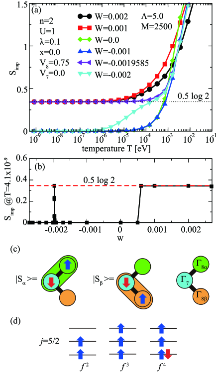
Figure 3: (Color online) (a) Entropies for $n=2$ and $V_{7}=0$ on the line of $B_{4}^{0}=0$. Here we set $x=0$ and change $W$ between $W=-0.002$ and $0.002$. (b) Residual entropies at $T=4.1\times 10^{-9}$ vs. $W$ for $x=0$. (c) Schematic views for the major components of the local $\Gamma_{3}$ states in the $j$-$j$ coupling scheme. Note that the oval symbolically indicates the singlet state between $\Gamma_{7}$ and $\Gamma_{8}$ orbitals. (d) Electron configurations in the $j$-$j$ coupling scheme for $n=2$, $3$, and $4$. Here we accommodate electrons with pseudo-spins (blue up and red down) in the $j=5/2$ sextet.

Before proceedings to the discussion on the results for the three-band case, let us review our previous results for the two-band model, corresponding to the case for $V_{7}=0$ and $V_{8}\neq 0$. [26, 28, 30] First we consider the case of Pr³⁺ ion with $n=2$.[28] In Fig. 3(a), we depict some results of $f$-electron entropies, when we change the values of $W$ for $x=0$ from $W=0.002$ ($\Gamma_{3}$ doublet) to $W=-0.002$ ($\Gamma_{1}$ singlet). For $W=0.002$ and $0.001$, we observe a residual entropy of $0.5\log 2$ at low temperatures, suggesting the appearance of the two-channel Kondo effect.

Here we turn our attention to Fig. 3(b), in which we show residual entropies at $T=4.1\times 10^{-9}$ for $-0.0027\leq W\leq 0.0027$. When we decrease $W$ from $W=0.0027$ to $0$ through $W=0.001$, we observe that the entropy suddenly becomes zero from $0.5\log 2$ at $W\approx 5.0\times 10^{-4}$ between $W=0.001$ and $W=0$, suggesting the change from the two-channel Kondo to the local Fermi-liquid phases. Note that the local $\Gamma_{3}$ state is found for $W>0$, as shown in Fig. 2(a), but due to the hybridization effect, the singlet phase is obtained even for $W>0$. Here we emphasize that the entropy change seems to occur discontinuously and anomalous behavior does not appear in the region between two-channel Kondo and Fermi-liquid phases.

Prior to the discussion on the results in the region of $W<0$, let us discuss the mechanism of the two-channel Kondo effect. As mentioned in Sect. 1, Cox explained that the two-channel Kondo effect occurs due to the exchange of $\Gamma_{3}$ quadrupole degrees of freedom,[4] but we emphasize that it is quite useful to interpret such a picture on the basis of a $j$-$j$ coupling scheme.[28] The local CEF states are composed of the electrons in the $j=5/2$ and $7/2$ states, but they are well approximated by two-electron states among the $j=5/2$ sextet. Then, the local $\Gamma_{3}$ states are well described by

$$\begin{split}|\Gamma_{3\alpha}\rangle&\approx\sqrt{\frac{16}{21}}|S_{\alpha}\rangle+\sqrt{\frac{5}{21}}|S_{8}^{(1)}\rangle,\\ |\Gamma_{3\beta}\rangle&\approx\sqrt{\frac{16}{21}}|S_{\beta}\rangle+\sqrt{\frac{5}{21}}|S_{8}^{(2)}\rangle,\end{split}$$ (14)

where the major components, $|S_{\alpha}\rangle$ and $|S_{\beta}\rangle$, indicate the singlets between $\Gamma_{7}$ and $\Gamma_{8}$ orbitals, whereas the minor components, $|S_{8}^{(1)}\rangle$ and $|S_{8}^{(2)}\rangle$, denote the singlets composed of two $\Gamma_{8}$ electrons. As schematically shown in Fig. 3(c), $|S_{\alpha}\rangle$ and $|S_{\beta}\rangle$ are, respectively, given by

$$\begin{split}|S_{\alpha}\rangle&=\sqrt{\frac{1}{2}}\left(f^{{\dagger}}_{a\gamma\uparrow}f^{{\dagger}}_{a\alpha\downarrow}-f^{{\dagger}}_{a\gamma\downarrow}f^{{\dagger}}_{a\alpha\uparrow}\right)|0\rangle,\\ |S_{\beta}\rangle&=\sqrt{\frac{1}{2}}\left(f^{{\dagger}}_{a\gamma\uparrow}f^{{\dagger}}_{a\beta\downarrow}-f^{{\dagger}}_{a\gamma\downarrow}f^{{\dagger}}_{a\beta\uparrow}\right)|0\rangle.\end{split}$$ (15)

On the other hand, $|S_{8}^{(1)}\rangle$ and $|S_{8}^{(2)}\rangle$ are given by

$$\begin{split}|S_{8}^{(1)}\rangle&=\sqrt{\frac{1}{2}}\left(f^{{\dagger}}_{a\beta\uparrow}f^{{\dagger}}_{a\beta\downarrow}-f^{{\dagger}}_{a\alpha\uparrow}f^{{\dagger}}_{a\alpha\downarrow}\right)|0\rangle,\\ |S_{8}^{(2)}\rangle&=\sqrt{\frac{1}{2}}\left(f^{{\dagger}}_{a\alpha\uparrow}f^{{\dagger}}_{a\beta\downarrow}-f^{{\dagger}}_{a\alpha\downarrow}f^{{\dagger}}_{a\beta\uparrow}\right)|0\rangle,\end{split}$$ (16)

respectively.

As mentioned above, the major components of the local $\Gamma_{3}$ states are given by the singlets between $\Gamma_{7}$ and $\Gamma_{8}$ orbitals. This picture of the composite degree of freedom is useful to promote our understanding on the quadrupole two-channel Kondo effect. Here we note that the $\Gamma_{3}$ states are classified by the orbital degree of freedom in $\Gamma_{8}$, since $\Gamma_{8}$ is isomorphic to the direct product of $\Gamma_{6}$ and $\Gamma_{3}$. When we introduce orbital operators $\mib{T}$ and $\mib{\tau}_{\sigma}$ to express the local $\Gamma_{3}$ state and $\Gamma_{8}$ conduction electron with pseudo-spin $\sigma$, respectively,[28] we obtain the exchange term as $J(\mib{\tau}_{\uparrow}+\mib{\tau}_{\downarrow})\cdot\mib{T}$ with the anti-ferro orbital exchange interaction $J$, leading to the same model as that of Noziéres and Blandin.[3]

Now let us return to Fig. 3(a). When we further decrease $W$ from $W=0$ in the range of $W<0$, we find a signal of the appearance of QCP. Namely, both for $W=-0.001$ and $-0.002$, the entropy is zero at low temperatures, while at $W=-0.0019585$, we numerically observe the residual entropy of $0.5\log 2$ at low temperatures. Note that this entropy immediately disappears when we change the value of $W$ even slightly, as we observe in the result for $W=-0.002$. As shown in Fig. 3(b), the entropies at $T=4.1\times 10^{-9}$ are zeros and we find a sharp peak at $W=-0.0019585$. This is the well-known quantum critical behavior emerging between CEF singlet and Kondo singlet phases. [9, 10, 11, 12, 13, 14, 15, 16, 17, 18, 19, 20, 21, 22, 23, 24, 25, 26, 27, 28, 29, 30] Here we show only the QCP on the line of $B_{4}^{0}=0$, but this QCP is considered to form the curve along the boundary between $\Gamma_{1}$ and $\Gamma_{5}$ ground states in Fig. 2(a). We note that the quantum critical curve always appears in the $\Gamma_{1}$ region. Note also that the curve seems to merge to the two-channel Kondo phase.

Here we provide a short comment on the emergence of two-channel Kondo effect for $n=4$.[30] It is useful to consider the $f^{4}$-electron configurations in the $j$-$j$ coupling scheme. As schematically shown in Fig. 3(d), when we accommodate four $f$ electrons in the $j=5/2$ sextet, we find two $f$ holes there. Namely, the electron-hole relation between $n=2$ and $n=4$ approximately holds on the basis of the $j$-$j$ coupling scheme. Thus, we expect to observe the quadrupole two-channel Kondo effect even for $n=4$, corresponding to Np³⁺ and Pu⁴⁺ ions.[30]

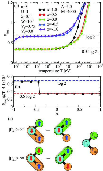
Figure 4: (Color online) (a) Entropies for $n=3$ and $V_{7}=0$ on the lines of $W=0.001$ and $-1\leq x\leq 1$. (b) Residual entropies at $T=4.1\times 10^{-9}$ vs. $x$ for $W=0.001$. (c) Schematic views for the main components of the local $\Gamma_{6}$ states in the $j$-$j$ coupling scheme.

Now we consider the case of Nd³⁺ ion with $n=3$.[26] In Fig. 4(a), we depict some results of $f$-electron entropies, when we change the values of $x$ for $W=0.001$ from $x=1$ ($\Gamma_{6}$ doublet) to $x=-1$ ($\Gamma_{8}$ quartet). For $x=1$, $0.5$, and $0$, we observe residual entropies of $0.5\log 2$ at low temperatures, indicating the two-channel Kondo effect. For $x=-0.5$ and $x=-1$, we find entropy plateaus with the value near $\log 2$, but they are eventually released for $T<10^{-9}$.

In Fig. 4(b), we show residual entropies at $T=4.1\times 10^{-9}$ between $-1\leq x\leq 1$. For $-0.4\leq x\leq 1$, we observe the residual entropy of $0.5\log 2$, suggesting the appearance of two-channel Kondo effect. At $x\approx 0.4$, the residual entropy of $0.5\log 2$ seems to change suddenly to the value near $\log 2$. Roughly speaking, the region with residual entropy $\log 2$ corresponds to that of $\Gamma_{8}$ quartet in Fig. 2(b). The $\Gamma_{8}$ quartet is approximately obtained by the addition of one $\Gamma_{8}$ electron to the double occupied $\Gamma_{7}$ states on the basis of the $j$-$j$ coupling scheme. When we include the hybridization with $\Gamma_{8}$ conduction electrons, we understand the appearance of the Kondo effect, since the $\Gamma_{7}$ degree of freedom is suppressed. Thus, the residual entropy near $\log 2$ in Fig. 4(b) should be eventually released when we decrease the temperature, leading to the Fermi-liquid state.

To understand the two-channel Kondo effect emerging from the $\Gamma_{6}$ doublet, it is again useful to consider the $\Gamma_{6}$ states on the basis of the $j$-$j$ coupling scheme. After some algebraic calculations, the major components of the $\Gamma_{6}$ states are found to be expressed by three pseudo-spins on $\Gamma_{7}$ and $\Gamma_{8}$ orbitals, as shown in Fig. 4(c). Namely, we obtain [26, 38]

$$\begin{split}|\Gamma_{6},\uparrow\rangle&=\sqrt{\frac{1}{3}}\left(f^{{\dagger}}_{a\alpha\uparrow}|S_{\beta}\rangle-f^{{\dagger}}_{a\beta\uparrow}|S_{\alpha}\rangle\right),\\ |\Gamma_{6},\downarrow\rangle&=\sqrt{\frac{1}{3}}\left(f^{{\dagger}}_{a\alpha\downarrow}|S_{\beta}\rangle-f^{{\dagger}}_{a\beta\downarrow}|S_{\alpha}\rangle\right).\end{split}$$ (17)

As discussed above, the main components of the $\Gamma_{3}$ doublet states for $n=2$ are expressed by $|S_{\alpha}\rangle$ and $|S_{\beta}\rangle$. Then, we obtain the $\Gamma_{6}$ doublet states for $n=3$ by adding one $\Gamma_{8}$ electron to the $\Gamma_{3}$ states for $n=2$, as shown in Fig. 4(c).

As emphasized in Ref. Hotta1, on the basis of the local $\Gamma_{6}$ states composed of three pseudo-spins, we envisage a picture that the local $\Gamma_{7}$ pseudo-spin is screened by $\Gamma_{8}$ electrons, when we include the hybridization between localized and conduction $\Gamma_{8}$ electrons. The present picture has been actually explained by the extended $s$-$d$ model.[26] We believe that it is the realization of the magnetic two-channel Kondo effect, originally raised by Noziéres and Blandin.[3]

4 Calculation Results for the Three-Band Model

4.1 Results for $n=2$: Effect of CEF potentials

Now we show our present results for the three-band case with $V_{7}=V_{8}=V$. In this subsection, let us discuss the effect of CEF potentials on the emergence of QCP for the case of $n=2$. In Fig. 5(a), we pick up some results when we change the CEF parameters from $x=0$ ($\Gamma_{3}$ doublet) to $x=1$ ($\Gamma_{1}$ singlet) for $W=0.001$. In Fig. 5(b), we plot $S_{\rm imp}$ at $T=7.5\times 10^{-9}$ as a function of $x$.

For $x=0$ and $0.17$, we find a residual entropy of $0.5\log 2$ at low temperatures, suggesting the appearance of the two-channel Kondo effect, even when we consider the hybridization with $\Gamma_{7}$ band in addition to those with $\Gamma_{8}$ bands. It is useful to consider the local $\Gamma_{3}$ states on the basis of the $j$-$j$ coupling scheme, as shown in Fig. 3(c). Namely, the doublet is expressed by the composite states, which are two singlets between $\Gamma_{7}$ and $\Gamma_{8}$ orbitals. When the hybridization occurs only between $\Gamma_{8}$orbitals, there appear anti-ferro exchange interactions in terms of orbital degree of freedom between localized and conduction $\Gamma_{8}$ electrons, whereas pseudo-spin plays a role of channel. In this case, the localized $\Gamma_{7}$ orbital plays no role in the hybridization process, after the formation of the singlet between $\Gamma_{7}$ and $\Gamma_{8}$ electrons.

When we further include the hybridization of $\Gamma_{7}$, there appears a process in which the singlets composed of $\Gamma_{3}$ doublets are destroyed by the formation of another singlet between localized and conduction $\Gamma_{7}$ electrons. Thus, we envision the competition between $\Gamma_{7}-\Gamma_{7}$ and $\Gamma_{7}-\Gamma_{8}$ singlets, leading to a QCP. For the three-band case, there occurs three channels, in which two of them are $\Gamma_{8}$ pseudo-spins and another is $\Gamma_{7}$ orbital, as schematically shown in Fig. 5(c).

Here we consider the case of $V_{7}\gg V_{8}$, in which the two-channel Kondo phase should be suppressed, since the singlets composed of $\Gamma_{3}$ doublets are considered to be destroyed by the screening of the $\Gamma_{7}$ pseudo-spin. In fact, in the limit of $V_{8}=0$, it is easy to imagine the appearance of the underscreening Kondo effect concerning the $\Gamma_{7}$ pseudo-spin with localized $\Gamma_{8}$ quartet. Thus, we deduce that there appears additional $\Gamma_{7}$ orbital channel in the two-channel Kondo phase for the three-band case.

Next we turn our attention to the results for $x=0.2$ and $0.3$ in Fig. 5(a). Although these $x$ values for $W=0.001$ are included in the $\Gamma_{3}$ doublet in Fig. 1, it seems that we arrive at the singlet phase due to the hybridization effect, since the residual entropy becomes zero. It is difficult to prove the Fermi-liquid phase only by the entropy results, but we deduce it also from the energy spectrum data.

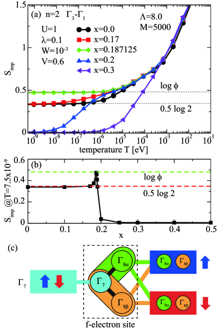
Figure 5: (Color online) (a) Entropies for $n=2$, $W=0.001$, and $0\leq x\leq 0.3$ between $\Gamma_{3}$ and $\Gamma_{1}$. (b) Residual entropies at $T=7.5\times 10^{-9}$ vs. $x$ for $W=0.001$. (c) Schematic view for the three channels when the local $\Gamma_{3}$ states are hybridized with three conduction bands for $n=2$.

Now we focus on the result at $x=0.187125$, in which we find a residual entropy, suggesting the unstable fixed point. In fact, it disappears when we slightly change $x$. We call it the $\Gamma_{3}-\Gamma_{1}$ QCP, but the value of the residual entropy should be carefully discussed. It is between $0.5\log 2$ and $\log 2$, but at first glance, we could not understand the meaning of that value. Here we recall that the QCP between two different Fermi-liquid phases is characterized by the residual entropy of $0.5\log 2$, equal to that for the two-channel Kondo effect. Then, we hit upon a simple idea that the QCP between two-channel Kondo and Fermi-liquid phases is characterized by the residual entropy equal to that for the three-channel Kondo effect. The analytic value of the residual entropy $S_{\rm ana}$ for multi-channel Kondo effect is given by [39]

$$S_{\rm ana}=\log\frac{\sin[(2S+1)\pi/(n_{\rm c}+2)]}{\sin[\pi/(n_{\rm c}+2)]},$$ (18)

where $S$ denotes the impurity spin and $n_{\rm c}$ indicates the channel number. In the present case, the $\Gamma_{3}$ doublet is effectively expressed by $S=1/2$ and we obtain $n_{\rm c}=3$ with two pseudo-spins and one orbital, as shown in Fig. 5(c). Thus, we obtain $S_{\rm ana}=\log\phi$ with the golden ratio $\phi=(1+\sqrt{5})/2$.

From the numerical results shown by green circles in Fig. 5(a), we obtain $S_{\rm imp}=0.472$ at $T=7.5\times 10^{-9}$, which is deviated from the analytic value $S_{\rm ana}=0.481$. For the two-channel Kondo phase at $x=0$, we find $S_{\rm imp}=0.339$ at $T=7.5\times 10^{-9}$, which is also deviated from the analytic value $S_{\rm ana}=0.5\log 2=0.347$. This deviation inevitably occurs in the NRG calculation due to $\Lambda$ larger than unity and finite $M$. Note that the deviation becomes large for $\Lambda>8$ when we fix $M$ as $M=5,000$. We consider that the result at $x=0.187125$ suggests the unstable fixed point characterized by the entropy $\log\phi$. Note that this type of QCP was pointed out in a three-orbital impurity Anderson model for a single C₆₀ molecule.[20]

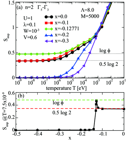
Figure 6: (Color online) (a) Entropies for $n=2$, $W=0.001$, and $-0.3\leq x\leq 0$ between $\Gamma_{3}$ and $\Gamma_{5}$. (b) Residual entropies at $T=7.5\times 10^{-9}$ vs. $x$ for $W=0.001$.

Let us now turn our attention to Fig. 5(b), in which we show $S_{\rm imp}$ at $T=7.5\times 10^{-9}$ as a function of $x$ to confirm the critical behavior. We clearly find a sharp peak with the value of $\log\phi$ between the two-channel Kondo region characterized by the entropy of $0.5\log 2$ and the Fermi-liquid phase characterized by zero entropy. From these results, it is highly believed that an important aspect of the QCP is captured, although we recognize that the existence of QCP is not rigorously proved by the present results.

If the QCP appears between two-channel Kondo and Fermi-liquid phases, the emergence of the QCP should not be limited to the region between $\Gamma_{3}$ doublet and $\Gamma_{1}$ singlet. In Fig. 6(a), we show some results when we change the CEF parameters from $x=0$ ($\Gamma_{3}$ doublet) to $x=-1$ ($\Gamma_{5}$ triplet) for $W=0.001$. For $x=0$ and $-0.1$, we obtain the two-channel Kondo phase, while for $x=-0.3$ and $-0.2$, the screened Kondo phase appears, since in a $j$-$j$ coupling scheme, the local $\Gamma_{5}$ triplet is mainly composed of two $\Gamma_{8}$ electrons, which are screened by $\Gamma_{8}$ conduction electrons. Between two-channel Kondo and screened Kondo phases, we again find the residual entropy of $\log\phi$ at $x=-0.12771$. As shown in Fig. 6(b), the entropies at $T=7.5\times 10^{-9}$ suggest the QCP as a sharp peak, which defines the $\Gamma_{3}-\Gamma_{5}$ QCP. Thus, we guess that the QCP characterized by the residual entropy of $\log\phi$ generally appears between two-channel Kodno and Fermi-liquid phases.

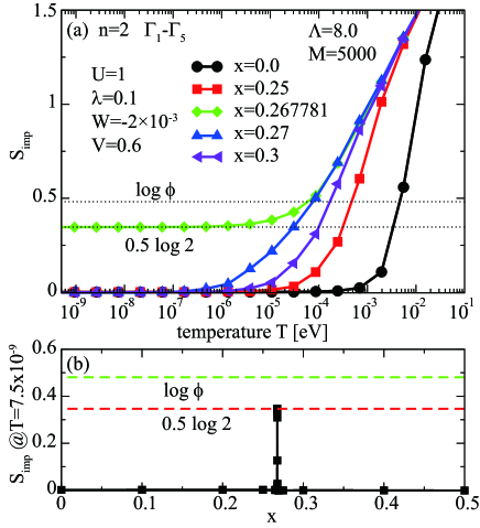
Figure 7: (Color online) (a) Entropies for $n=2$, $W=-0.002$, and $0\leq x\leq 0.3$ between $\Gamma_{5}$ and $\Gamma_{1}$. (b) Residual entropies at $T=7.5\times 10^{-9}$ vs. $x$ for $W=-0.002$.

Although we observe the $\Gamma_{3}-\Gamma_{5}$ QCP characterized by $\log\phi$ between two-channel Kondo and screened Kondo phases, it does not immediately mean that the property of the $\Gamma_{3}-\Gamma_{5}$ QCP is the same as that of the $\Gamma_{3}-\Gamma_{1}$ QCP between two-channel Kondo and CEF singlet phases. In particular, from a microscopic viewpoint, we are interested in the kinds of the three channels on the QCP. As for the $\Gamma_{3}-\Gamma_{1}$ QCP, we consider that two of the three channels are pseudo-spins and another is orbital, as shown in Fig. 5(c) for the three-channels in the two-channel Kondo effect emerging from the local $\Gamma_{3}$ states. Here we believe that the three channels on the $\Gamma_{3}-\Gamma_{5}$ QCP are the same as those on the $\Gamma_{3}-\Gamma_{1}$ QCP, but unfortunately, we cannot prove it exactly in this study. As mentioned above, the local $\Gamma_{5}$ triplet mainly composed of a couple of $\Gamma_{8}$ electrons should be screened by $\Gamma_{8}$ conduction electrons. Thus, we cannot deny a possibility that all three channels on the $\Gamma_{3}-\Gamma_{5}$ QCP may be related to orbital degrees of freedom. At the present stage, it is phenomenologically shown that the QCP characterized by $\log\phi$ appears between two-channel Kondo and Fermi-liquid phases. The properties of the $\Gamma_{3}-\Gamma_{1}$ and $\Gamma_{3}-\Gamma_{5}$ QCP’s are not completely clarified, but we will mention this point later again.

Now we turn our attention to the QCP between CEF singlet and screened Kondo singlet phases, when we include the hybridization with three conduction bands. In Fig. 7(a), we pick up some results when we change the CEF parameters from $x=0$ ($\Gamma_{1}$ singlet) to $x=1$ ($\Gamma_{5}$ triplet). Note that here we use $|W|=0.002$ to emphasize the critical behavior. For $x=0$ and $0.25$, we find the CEF singlet phase, while for $x=0.27$ and $0.3$, the screened Kondo singlet phase appears. At $x=0.267781$, we observe the residual entropy of $0.5\log 2$, as we have expected from the QCP between two different Fermi-liquid phases. As shown in Fig. 7(b), we observe a sharp peak with the value of $0.5\log 2$ around at $x\approx 0.27$. Note again that the local $\Gamma_{5}$ triplet mainly composed of two $\Gamma_{8}$ electrons is screened by $\Gamma_{8}$ conduction electrons. Thus, the $\Gamma_{8}$ conduction electrons play main roles and the $\Gamma_{7}$ degree of freedom is considered to be irrelevant on the QCP between two Fermi-liquid phases even in the three-band case.

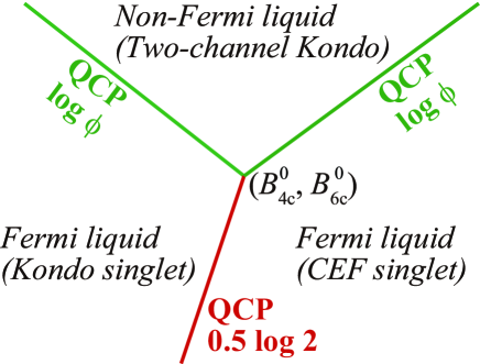
Figure 8: (Color online) Schematic view for the phase diagram on the $(B_{4}^{0},B_{6}^{0})$ plane, deduced from the NRG results in Figs. 5, 6, and 7.

To summarize this subsection, we depict a schematic view for the phase diagram on the $(B_{4}^{0},B_{6}^{0})$ plane in Fig. 8 on the basis of the results in Figs. 5, 6, and 7. Between two-channel Kondo and Fermi-liquid (CEF singlet or screened Kondo singlet) phases, we deduce the appearance of the line of QCP characterized by $\log\phi$. On the other hand, we expect another QCP line characterized by $0.5\log 2$ between two different Fermi-liquid phases.

We believe that the schematic phase diagram in Fig. 8 grasps the essential points on the $(B_{4}^{0},B_{6}^{0})$ plane, but we do not prove the existence of the point $(B_{4{\rm c}}^{0},B_{6{\rm c}}^{0})$ at which three QCP lines are connected to one another. Here we mention $(B_{4{\rm c}}^{0},B_{6{\rm c}}^{0})\neq(0,0)$ due to the effect of hybridizations, since the boundary curves are deviated from those among local CEF ground states as shown in Fig. 2(a). For instance, the region of the two-channel Kondo phase is not exactly equal to that of the local $\Gamma_{3}$ state and the QCP line characterized by $0.5\log 2$ always appears in the region of the local $\Gamma_{1}$ state.

In a phenomenological level, we believe that the kinds of the three channels on the $\Gamma_{3}-\Gamma_{5}$ QCP are the same as those on the $\Gamma_{3}-\Gamma_{1}$ QCP, since both are characterized by the residual entropy $\log\phi$. It may be possible to clarify this issue when we investigate the quantum critical behavior in the vicinity of the point of $(B_{4{\rm c}}^{0},B_{6{\rm c}}^{0})$. It is one of future problems.

4.2 Results for $n=2$: Effect of hybridization

Next we consider the effect of the hybridization on the emergence of QCP by monitoring the entropies for the fixed values of CEF parameters. First we consider the case of $V_{7}=V_{8}=V$. In Fig. 9(a), we show the entropies by changing $V$ from $V=0.57$ to $V=0.7$ for $n=2$, $W=0.001$, and $x=0$. In Fig. 9(b), we plot $S_{\rm imp}$ at $T=7.5\times 10^{-9}$ as a function of $x$.

Now we pay our attention to the results for $V=0.57$ and $0.6$, in which we observe the residual entropy near the value of $0.5\log 2$ at $T=7.5\times 10^{-9}$, suggesting the existence of the two-channel Kondo phase, while for $V=0.615$ and $0.7$, we obtain the Fermi-liquid phase, since the entropies are eventually released. Note that in the present paper, we do not further discuss the entropy behavior for $V$ smaller than $0.57$. At $V=0.607841$, we again observe the QCP characterized by $\log\phi$. This result is considered to reconfirm the emergence of QCP induced by the hybridization between two-channel Kondo and Fermi-liquid phases.

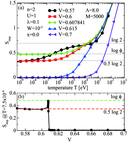
Figure 9: (Color online) (a) Entropies for $n=2$ and $0.57\leq V\leq 0.7$ with $W=0.001$ and $x=0$. (b) Residual entropies at $T=7.5\times 10^{-9}$ vs. $V$ for $W=0.001$ and $x=0$.

Next we discuss the emergence of the QCP characterized by $\log\phi$ for the case of $V_{7}\neq V_{8}$. Here we shortly discuss two limiting situations, $V_{7}=0$ and $V_{8}=0$. The former case of $V_{7}=0$ corresponds to the two-band model, as discussed in Sect. 3. Namely, the two-channel Kondo effect has been confirmed to appear in the region of the local $\Gamma_{3}$ state for an appropriate value of $V_{8}$. As shown later, when we increase the value of $V_{8}$ for the case of $V_{7}=0$, we do not observe the QCP characterized by $\log\phi$ between two-channel Kondo and Fermi-liquid phases in the NRG results, as shown later.

The case of $V_{8}=0$ apparently corresponds to the one-band model, in which the underscreening Kondo effect is expected to occur. Here it is useful to recall that the local $\Gamma_{3}$ is expressed by the singlets between $\Gamma_{7}$ and $\Gamma_{8}$ electrons. For small $V_{7}$, the local $\Gamma_{3}$ doublet remains even at low temperatures, leading to a residual entropy of $\log 2$, when we consider the hybridization of $\Gamma_{7}$ electrons. On the other hand, for large $V_{7}$, the $\Gamma_{7}$ pseudo-spin in the local $\Gamma_{3}$ singlets is screened by $\Gamma_{7}$ conduction electrons, leading to a residual entropy of $\log 4$ originating from the remaining $\Gamma_{8}$ electron. In any case, for the case of $V_{8}=0$, we do not expect the appearance of the two-channel Kondo effect.

When we turn our attention to the case of $V_{7}\neq 0$ and $V_{8}\neq 0$, it is intuitively considered that the QCP appearing for the case of $V_{7}=V_{8}=V$ should not disappear immediately even when $V_{7}$ becomes different from $V_{8}$. Furthermore, we expect that the QCP still appears for a certain critical value of $V_{8}$ for the case of small $V_{7}$.

In Fig. 10(a), we show some results when we change the value of $V_{8}$ from $V_{8}=0.8$ to $V_{8}=0.85$ for $V_{7}=0.1$ with $W=0.001$ and $x=0$. For $V_{8}=0.8$ and $0.815$, we obtain the two-channel Kondo phase, suggested from the residual entropy of $0.5\log 2$, while for $V_{8}=0.825$ and $0.85$, the Fermi-liquid phase appears. Between two-channel Kondo and Fermi-liquid phases, we find the residual entropy of $\log\phi$ at $V_{8}=0.81936$. As shown in Fig. 10(b), we observe the QCP as a sharp peak in the entropies at $T=7.5\times 10^{-9}$.

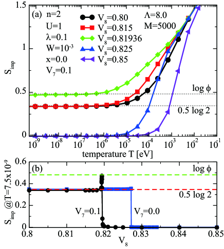
Figure 10: (Color online) (a) Entropies for $n=2$ and $0.8\leq V_{8}\leq 0.85$ for $V_{7}=0.1$, $W=0.001$, and $x=0$. (b) Residual entropies at $T=7.5\times 10^{-9}$ vs. $V_{8}$ for $V_{7}=0$ (blue solid square) and $0.1$ (black solid circle). Other parameters are the same as those in (a).

In Fig. 10(b), we also show the entropies for the case of $V_{7}=0$. Note here that we perform the NRG calculations with $\Lambda=8$ and $M=5,000$ even for the two-band case to keep the same conditions as those for the three-band case. In this case, we do not observe a characteristic peak with the value of $\log\phi$ between two-channel Kondo and Fermi-liquid phases. Rather we find a sudden change from $0.5\log 2$ to zero in the two-band case at $V_{8}=V_{8}^{*}=0.8272$. This is consistent with Fig. 3(b), showing the residual entropies when we change $W$ with $x=0$. When we compare the results for $V_{7}\neq 0$ and $V_{8}\neq 0$ with those for $V_{7}=0$ and $V_{8}\neq 0$, we imagine that the hybridization with $\Gamma_{7}$ band is indispensable for the appearance of the QCP characterized by the entropy of $\log\phi$.

4.3 Results for $n=3$

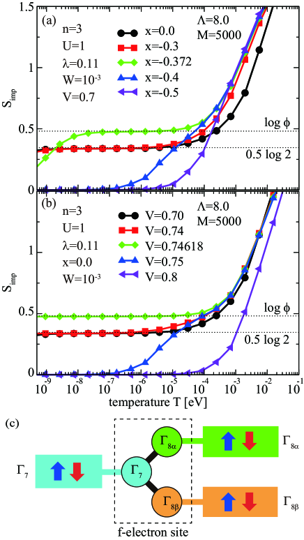
Figure 11: (Color online) (a) Entropies for $W=10^{-3}$ and $-0.5\leq x\leq 0$. Here we set $V=0.7$. (b) Entropies for $0.5\leq V\leq 0.8$. Here we fix $x=0.0$ and $W=10^{-3}$. (c) Schematic view for the three channels when the local $\Gamma_{6}$ states are hybridized with three conduction bands for $n=3$.

Thus far, we have considered the QCP near the quadrupole two-channel Kondo phase for the case of $n=2$. To confirm our idea that the QCP appears between two-channel Kondo and Fermi-liquid phases, in this subsection, we show our NRG results for the case of $n=3$. As mentioned in Sect. 3, it has been shown that the magnetic two-channel Kondo effect occurs in the $\Gamma_{6}$ doublet for the two-band case.[26]

In Fig. 11(a), we show some results when we change the CEF parameters from $x=0$ ($\Gamma_{6}$ doublet) to $x=-1$ ($\Gamma_{8}$ quartet) for $n=3$, $W=0.001$, and $V=0.7$. For $x=0$ and $-0.3$, we obtain the magnetic two-channel Kondo phase, while for $x=-0.4$ and $-0.5$, the screened Kondo phase appears, since the $\Gamma_{8}$ quartet effectively expressed by $S=3/2$ spin is screened by three conduction electrons. At $x=-0.372$ between two-channel Kondo and Fermi-liquid phases, we find an entropy plateau of $\log\phi$. In this case, we could not observe the residual entropy of $\log\phi$ at low enough temperatures, but the signal of QCP is considered to be obtained.

In Fig. 11(b), we show the results for $f$-electron entropies when we change $V$ for $n=3$, $W=0.001$, and $x=0$. For $V=0.7$ and $0.74$, we clearly observe a residual entropy $0.5\log 2$, suggesting the two-channel Kondo effect, while for $V=0.75$ and $0.8$, we find the local singlet phases, suggesting the Fermi-liquid states. Between those two phases, at $V=0.74618$, we again observe the residual entropy characterized by $\log\phi$. These results for $n=3$ strongly suggest that the emergence of QCP between magnetic two-channel Kondo and Fermi-liquid phases.

Concerning the three channels on the QCP, it is again useful to recall the local $\Gamma_{6}$ doublet on the basis of the $j$-$j$ couplings scheme, as shown in Fig. 4(c). As mentioned in Sect. 3, we have understood the magnetic two-channel Kondo effect for $n=3$ by considering that the $\Gamma_{7}$ pseudo-spin is screened by $\Gamma_{8}$ electrons. In Fig. 11(c), we schematically show the figure for the three channels in the two-channel Kondo effect emerging from the local $\Gamma_{6}$ states for $n=3$. When we further include the effect of hybridization of $\Gamma_{7}$ electron, we envisage a picture that the $\Gamma_{7}$ pseudo-spin is screened by $\Gamma_{8}$ and $\Gamma_{7}$ electrons. Namely, on the QCP characterized by $\log\phi$ for $n=3$, impurity spin $S$ in Eq. (18) denotes the $\Gamma_{7}$ pseudo-spin and all three channels ($n_{\rm c}=3$) are given by orbital degrees of freedom.

5 Discussion and Summary

In this paper, we have analyzed the seven-orbital impurity Anderson model hybridized with three ($\Gamma_{7}$ and $\Gamma_{8}$) conduction bands with the use of the NRG method. For Pr³⁺ and Nd³⁺ ions, we have evaluated the $f$-electron entropies by controlling CEF potentials and hybridization magnitudes. Then, we have found the QCP characterized by the residual entropy of $\log\phi$ between two-channel Kondo and Fermi-liquid phases.

We believe that the emergence of this QCP does not depend on the nature of the two-channel Kondo phase, quadrupole or magnetic, and also the details of the Fermi-liquid phase, CEF or Kondo singlets. As for the three channels the QCP, they are considered to depend on the property of the two-channel Kondo phase. Namely, for $n=2$, the three channels are two pseudo-spins of $\Gamma_{8}$ and one orbital of $\Gamma_{7}$, whereas for $n=3$, they are three orbitals of $\Gamma_{8}$ and $\Gamma_{7}$. Note that for $n=2$, the kinds of the three channels on the $\Gamma_{3}-\Gamma_{5}$ QCP are the same as those on the $\Gamma_{3}-\Gamma_{1}$ QCP. However, we cannot prove it in a microscopic level in the present study. For the purpose, it is necessary to promote our understanding on the phase diagram in Fig. 8 beyond the phenomenological level. This is one of future problems.

When we depict another phase diagram concerning the hybridization, the QCP characterized by $\log\phi$ is considered to form a curve on the $(V_{8},V_{7})$ plane. As mentioned above, this QCP does not appear for $V_{7}=0$ or $V_{8}=0$. For $V_{8}=0$, since the model is the one-band case, we can easily understand that the QCP does not appear. On the other hand, for the case of $V_{7}=0$, the two-channel Kondo phase is discontinuously changed to the Fermi-liquid phase at a certain value of $V_{8}^{*}$. The QCP curve for $V_{8}\neq 0$ and $V_{7}\neq 0$ seems to merge into the point at $V_{8}=V_{8}^{*}$ and $V_{7}=0$, but the fate of the QCP for the infinitesimal value of $V_{7}$ is unclear. This point will be investigated in future.

Furthermore, it is necessary to discuss the phase for small $V_{7}$ and $V_{8}$ with due care. This is the reason why we have not discussed the entropy behavior for small $V$ in Fig. 9. If the Fermi-liquid phase appears at this region, it may be different from that in the large hybridization region. In such a case, we expect another QCP curve characterized by $\log\phi$ depending on the CEF parameters. On the other hand, there is a possibility that the Fermi-liquid phase for large $V$ is connected to that for small $V$ when we consider the region of $V_{8}\neq V_{7}$. It is also a future problem to clarify the phase diagram on the $(V_{8},V_{7})$ plane.

In this paper, we have phenomenologically confirmed the QCP characterized by $\log\phi$ from the evaluation of the $f$-electron entropy, but it should be remarked that the existence of the QCP has not been proven exactly. To pile up the evidence, it is necessary to analyze other physical quantities. For instance, when we define a characteristic temperature $T^{*}$ at which the entropy $\log\phi$ is released, it is interesting to clarify the dependence of $T^{*}$ on the parameters of the model. This is also one of future tasks.

Finally, we briefly discuss a possibility to observe the present QCP in actual materials. If there exist Pr and/or Nd compounds in which the two-channel Kondo effect is observed, we propose to apply a high pressure to increase the hybridization $V$. When the pressure is increased, as expected from Fig. 3(b), we expect to observe quantum critical behavior in physical quantities at a critical pressure, different from that in the two-channel Kondo phase. At present, we cannot point out specific compounds, but we expect that Pr 1-2-20 and Nd 1-2-20 compounds may be candidates.

In summary, we have investigated the seven-orbital Anderson model hybridized with three conduction bands by using the NRG technique. We have observed the QCP characterized by $\log\phi$ between two-channel Kondo and Fermi-liquid phases, when we have controlled $n$, $V$, and CEF parameters. We hope that quantum critical behavior at this QCP can be found in cubic Pr and Nd compounds in which two-channel Kondo effect is observed.

References

- [1] J. Kondo, Prog. Theor. Phys. 32, 37 (1964).
- [2] B. Coqblin and J. R. Schrieffer, Phys. Rev. 185, 847 (1969).
- [3] Ph. Noziéres and A. Blandin, J. Physique 41, 193 (1980).
- [4] D. L. Cox, Phys. Rev. Lett. 59, 1240 (1987).
- [5] D. L. Cox and A. Zawadowski, Exotic Kondo Effects in Metals (Taylor & Francis, London, 1999), p. 24.
- [6] B. A. Jones and C. M. Varma, Phys. Rev. Lett. 58, 843 (1987).
- [7] B. A. Jones, C. M. Varma, and J. W. Wilkins, Phys. Rev. Lett. 61, 125 (1988).
- [8] B. A. Jones and C. M. Varma, Phys. Rev. B 40, 324 (1989).
- [9] M. Koga and H. Shiba, J. Phys. Soc. Jpn. 64, 4345 (1995).
- [10] M. Koga and H. Shiba, J. Phys. Soc. Jpn. 65, 3007 (1996).
- [11] H. Kusunose and K. Miyake, J. Phys. Soc. Jpn. 66, 1180 (1997).
- [12] H. Kusunose, J. Phys. Soc. Jpn. 67, 61 (1998).
- [13] Y. Shimizu, O. Sakai, and S. Suzuki, J. Phys. Soc. Jpn. 67, 2395 (1998).
- [14] M. Koga, G. Zaránd, and D. L. Cox, Phys. Rev. Lett. 83, 2421 (1999).
- [15] M. Koga, Phys. Rev. B 61, 395 (2000).
- [16] S. Yotsuhashi, K. Miyake, and H. Kusunose, J. Phys. Soc. Jpn. 71, 389 (2002).
- [17] M. Fabrizio, A. F. Ho, L. D. Leo, and G. E. Santoro, Phys. Rev. Lett. 91, 246402 (2003).
- [18] L. D. Leo and M. Fabrizio, Phys. Rev. B 69, 245114 (2004).
- [19] K. Hattori and K. Miyake, J. Phys. Soc. Jpn. 74, 2193 (2005).
- [20] L. D. Leo and M. Fabrizio, Phys. Rev. Lett. 94, 236401 (2005).
- [21] M. Koga and M. Matsumoto, Phys. Rev. B 77, 094411 (2008).
- [22] S. Nishiyama, H. Matsuura, and K. Miyake, J. Phys. Soc. Jpn. 79, 104711 (2010).
- [23] S. Nishiyama and K. Miyake, J. Phys. Soc. Jpn. 80, 124706 (2011).
- [24] A. K. Mitchell and E. Sela, Phys. Rev. B 85, 235127 (2012).
- [25] R. Shiina, J. Phys. Soc. Jpn. 86, 034705 (2017).
- [26] T. Hotta, J. Phys. Soc. Jpn. 86, 083704 (2017).
- [27] R. Shiina, J. Phys. Soc. Jpn. 87, 014702 (2018).
- [28] T. Hotta, Physica B 536C, 203 (2018).
- [29] M. Koga and M. Matsumoto, J. Phys. Soc. Jpn. 88, 034713 (2019).
- [30] D. Matsui and T. Hotta, JPS Conf. Proc. 30, 011125 (2020).
- [31] T. Onimaru and H. Kusunose, J. Phys. Soc. Jpn. 85, 082002 (2016).
- [32] K. G. Wilson, Rev. Mod. Phys. 47, 773 (1975).
- [33] H. R. Krishna-murthy, J. W. Wilkins, and K. G. Wilson, Phys. Rev. B 21, 1003 (1980).
- [34] M. T. Hutchings, Solid State Phys. 16, 227 (1964).
- [35] J. C. Slater, Quantum Theory of Atomic Structure (McGraw-Hill, New York, 1960).
- [36] T. Hotta and H. Harima, J. Phys. Soc. Jpn. 75, 124711 (2006).
- [37] K. R. Lea, M. J. M. Leask, and W. P. Wolf, J. Phys. Chem. Solids 23, 1381 (1962).
- [38] K. Kubo and T. Hotta, Phys. Rev. B 95, 054425 (2017).
- [39] I. Affleck and A. W. W. Ludwig, Nucl. Phys. B 360, 641 (1991).