Learning Functors using Gradient Descent

Abstract

Neural networks are a general framework for differentiable optimization which includes many other machine learning approaches as special cases. In this paper we build a category-theoretic formalism around a neural network system called CycleGAN [16]. CycleGAN is a general approach to unpaired image-to-image translation that has been getting attention in the recent years. Inspired by categorical database systems, we show that CycleGAN is a “schema”, i.e. a specific category presented by generators and relations, whose specific parameter instantiations are just set-valued functors on this schema. We show that enforcing cycle-consistencies amounts to enforcing composition invariants in this category. We generalize the learning procedure to arbitrary such categories and show a special class of functors, rather than functions, can be learned using gradient descent. Using this framework we design a novel neural network system capable of learning to insert and delete objects from images without paired data. We qualitatively evaluate the system on the CelebA dataset and obtain promising results.

1 Introduction

Compositionality describes and quantifies how complex things can be assembled out of simpler parts. It is a principle which tells us that the design of abstractions in a system needs to be done in such a way that we can intentionally forget their internal structure [9]. In the rapidly developing field of deep learning, there are two interesting properties of neural networks related to compositionality: (i) they are compositional – increasing the number of layers tends to yield better performance, and (ii) they are discovering (compositional) structures in data.

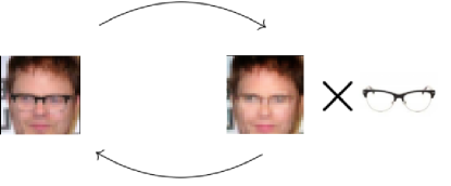
Figure 1: We devise a procedure to regularize neural network training when these networks are morphisms in a category presented by generators and relations. We use this regularization in the specific task of training neural networks to remove glasses from the face of a person and insert them parametrically. This is done without direct supervision and is object-invariant: the network is never provided with information that the image contains glasses or even that it contains a person.

A modern deep learning system is made up of different types of components: a neural network itself (a differentiable parameterized function; said to be learning during the process of optimization), an update rule, a cost/loss function (a differentiable function used to direct the learning and assess the performance of the network), and also often overlooked data cleaning and processing pipelines which supply the network with data.

In most deep learning setups the only component which is being optimized is, unsurprisingly, the neural network itself. However, this has seen a change in the recent years, where an increasing number of components of a modern deep learning system started being modified during learning. In many of these cases, these other components have been replaced by other neural networks which are trained and learned in parallel. For instance, Generative Adversarial Networks [7] also learn the cost function. The paper Learning to Learn by gradient descent by gradient descent [3] specifies networks that learn the update rule. The paper Decoupled Neural Interfaces using Synthetic Gradients [10] specifies how, surprisingly, even gradients themselves can be learned: in this case networks are reminiscent of agents which communicate information and gradient updates to each other.

These are just a few examples, but they give a sense of things to come. As more and more components of these systems stop being fixed throughout training, there is an increasingly larger need for more precise formal specification of the things that do stay fixed. This is not an easy task; the invariants across all these networks seem to be rather abstract and hard to describe. In this paper we explore the hypothesis that the language of category theory could be well suited to describe these systems in a compositional and precise manner.

Inter-domain mappings.

Recent advances in neural networks describe the process of discovering high-level, abstract structure in data using gradient information. As such, learning inter-domain mappings has received increasing attention in recent years, especially in the context of unpaired data and image-to-image translation [16, 2]. Pairedness of datasets $X$ and $Y$ generally refers to the existence of some invertible function $X\rightarrow Y$. Building datasets that contain that pairing information often requires extra human labor or computing resources. Moreover, many aspects of human learning do not involve paired datasets. As eloquently described in the introduction of [16], often we can reason about stylistic differences between paintings of different painters, even though never having seen paired data, i.e. the same scene painted by two different painters. This enables us to learn and generate high-level information from data well beyond the capabilities of many of the current learning algorithms.

Motivated by the success of Generative Adversarial Networks (GANs) [7] in image generation, some existing unsupervised learning methods [16, 2] use adversarial losses to learn the true data distribution of given domains of natural images and cycle-consistency losses to learn coherent mappings between those domains. CycleGAN is one of them. It is a system of neural networks which learns a one-to-one mapping between two domains. Each domain has an associated discriminator, while the mappings between these domains correspond to generators. It includes two notions of learning: i) adversarial learning, where generators and discriminators play the usual GAN minimax game [7], and ii) the cycle-consistency learning, where specific generator composition invariants are enforced. A commonly used example of this one-to-one mapping used in [16] is of images of horses and zebras. Simply by changing the texture of the animal in such an image we can, approximately, map back and forth between these images. Learning how to change this texture (without being provided the information that there are horses or zebras in the image) is what CycleGAN enables us to do.

Outline of the main contributions.

In this paper we make the first steps of formalization of general systems based on CycleGAN in the language of category theory.

We package CycleGAN into a category presented by generators and relations. Given such a category – which we call a schema, inspired by [14] – we specify the architectures of its constituent networks as a functor $\mathsf{Arch}$. We reason about various other notions found in deep learning, such as datasets, embeddings, and parameter spaces.

We associate the training process with an indexed family of functors $\{H_{p_{i}}:\mathbf{Free}(G)\rightarrow\mathbf{Set}\}_{i=1}^{T}$, where $T$ is the number of training steps and $p$ is some choice of a parameter for that architecture. Analogous to standard neural networks – starting with a randomly initialized $H_{p}$ we iteratively update it using gradient descent. The optimization is guided by generalized version of two objectives found in [16]: adversarial minimax objective and the cycle-consistency objective (also called here the path-equivalence objective).

This approach yields useful insights and a large degree of generality: (i) it enables learning with unpaired data as it does not impose any constraints on ordering or pairing of the sets in a category, and (ii) although specialized to generative models in the domain of computer vision, this approach is domain-independent and general enough to hold in any domain of interest, such as sound, text, or video. Roughly, this allows us to think of a subcategory of $\mathbf{Set}^{\mathbf{Free}(G)}$ as a space in which we can employ a gradient-based search. In other words, we use specific network composition invariants as regularization during training, such that the imposed relationships guide the learning process.

We show that for specific choices of $\mathbf{Free}(G)/{\sim}$ and the dataset we recover GAN [7] and CycleGAN [16]. Furthermore, we describe a novel neural network system capable of learning to remove and insert objects into an image with unpaired data (Figure 1). We qualitatively evaluate the system on the CelebA dataset and obtain promising results.

2 Towards Categorical Deep Learning

Modern deep learning optimization algorithms can be framed as a gradient-based search in some function space $Y^{X}$, where $X$ and $Y$ are sets that have been endowed with extra structure. Given some sets of data points $D_{X}\subseteq X$, $D_{Y}\subseteq Y$, a typical approach for adding inductive bias relies on exploiting this extra structure. This structure might be any sort of domain-specific features that can be exploited by various methods – convolutions for images, Fourier transform for audio, and specialized word embeddings for textual data.

In this paper we focus on a different sort of inductive bias - defined in [16] - where the inductive bias is increased not by exploiting extra structure of these sets, but rather by enforcing composition invariants of maps between those sets. We proceed by defining these schemas which contain the information about the ways these maps can be composed.

2.1 Model schema

Many deep learning models are complex systems, some comprised of several neural networks. Each neural network can be identified with domain $X$, codomain $Y$, and a differentiable parameterized function $X\rightarrow Y$. Given a collection of such networks, we use a directed multigraph to capture their interconnections. Each directed multigraph $G$ gives rise to a corresponding free category on that graph $\mathbf{Free}(G)$. Based on this construction, Figure 2 shows the interconnection pattern for generators of two popular neural network architectures: GAN [7] and CycleGAN [16].

no equations

(a) GAN

$g\circ f=\textrm{id}_{H}$
$f\circ g=\textrm{id}_{Z}$

(b) CycleGAN

Figure 2: Bird’s-eye view of two popular neural network systems

Observe that CycleGAN has some additional properties imposed on it, specified by equations in Figure 2 (b). These are called cycle-consistency conditions and can roughly be stated as follows: given domains $A$ and $B$ considered as sets, ${a\approx g(f(a)),\forall a\in A}$ and ${b\approx f(g(b)),\forall b\in B}$. A particularly clear diagram of the cycle-consistency condition can be found in [16, Figure 3.].

Our approach involves eta-reduction of the aforementioned equations to obtain ${id_{a}=g\circ f}$ and $id_{b}=f\circ g$. This allows us to package the newly formed equations as equivalence relations on the sets $\mathbf{Free}(G)(A,A)$ and $\mathbf{Free}(G)(B,B)$, respectively. This notion can be further packaged into a quotient category $\mathbf{Free}(G)/{\sim}$, together with the quotient functor ${\mathbf{Free}(G)\xrightarrow{Q}\mathbf{Free}(G)/{\sim}}$.

This formulation of CycleGAN – as a free category on a graph $G$ quotiented out by a specific equivalence relation – represents the cornerstone of our approach. These schemas allow us to precisely reason only about the interconnections between various concepts, while keeping any specific functions, networks or other some other sets separate. All the other constructs in this paper are structure-preserving maps between categories whose domain, roughly, can be traced back to $\mathbf{Free}(G)$.

2.2 What is a neural network?

In computer science, the idea of a neural network colloquially means a number of different things. At a most fundamental level, it can be interpreted as a system of interconnected units called neurons, each of which has a firing threshold acting as an information filtering system. Drawing inspiration from biology, this perspective is thoroughly explored in literature. In many other contexts we want to focus on the mathematical properties of a neural network and as such identify it with a function between sets $A\xrightarrow{f}B$. Those sets are always equipped with some notion of smoothness (most commonly Euclidean spaces). Functions are then considered to be maps of a given differentiability class which preserve such structure. We also frequently reason about a neural network jointly with its parameter space $P$ as a function of type $f:P\times A\rightarrow B$.

Without any loss of generality we illustrate how the learning in a neural network is done with a simple example. For instance, consider a classifier in the context of supervised learning. An example is a convolutional neural network whose input is a $32\times 32$ RGB image and output is real number, representing the probability of a cat appearing in the image. This network can be represented as a function with the following type: $\mathbb{R}^{n}\times\mathbb{R}^{32\times 32\times 3}\rightarrow\mathbb{R}$, for some $n\in\mathbb{N}$. In this case $\mathbb{R}^{n}$ represents the parameter space of this network.

In the machine learning community, a function of such type is commonly referred to as the neural network architecture. It specifies an entire parameterized family of functions of type $\mathbb{R}^{32\times 32\times 3}\rightarrow\mathbb{R}$, because partial application of each $p\in\mathbb{R}^{n}$ yields a function $f(p,-):\mathbb{R}^{32\times 32\times 3}\rightarrow\mathbb{R}$. This choice of a parameterized family of functions is part of the inductive bias we are building into the training process. For example, in computer vision it is common to restrict the class of functions to those that can be modeled by convolutional neural networks, while in natural language processing it is common to restrict to those functions modeled by recurrent neural networks. Each of these functions can be evaluated on how much it agrees with the data points. The process of learning, then, involves a priori specification of some such function $f:\mathbb{R}^{n}\times\mathbb{R}^{32\times 32\times 3}\rightarrow\mathbb{R}$ and some initial $p_{0}:\mathbb{R}^{n}$. By measuring how much the function agrees with our data points, we are able to “wiggle” that parameter $p_{0}$ and change it to the one that gives us a function which slightly better agrees with the data points.

With this in mind, we recall the model schema. For each morphism $A\rightarrow B$ in $\mathbf{Free}(G)$ we are interested in specifying a parameterized function $f:P\times A\rightarrow B$, i.e. a parameterized family of functions in $\mathbf{Set}$. The function $f$ describes a neural network architecture, and a choice of a partially applied $p\in P$ to $f$ describes a choice of some parameter value for that specific architecture.

We capture the notion of parametrization with the category $\mathbf{Para}$ [5]. It is a strict symmetric monoidal category whose objects are Euclidean spaces and morphisms $\mathbb{R}^{n}\rightarrow\mathbb{R}^{m}$ are equivalence classes of differentiable functions of type $\mathbb{R}^{p}\times\mathbb{R}^{n}\rightarrow\mathbb{R}^{m}$, for some $p$. Composition of morphisms in $\mathbf{Para}$ is defined in such a way that it explicitly keeps track of parameters. For more details, we refer the reader to [5].

A closely related construction we use is $\mathbf{Euc}$, the strict symmetric monoidal category whose objects are finite-dimensional Euclidean spaces and morphisms are differentiable maps. A monoidal product on $\mathbf{Euc}$ is given by the cartesian product. We package both of these notions – choosing an architecture and choosing parameters – into functors whose domain is $\mathbf{Free}(G)$ and codomains are $\mathbf{Para}$ and $\mathbf{Euc}$, respectively.

2.3 Network architecture

In the rest of the paper assume some directed multigraph $G$ has been specified and proceed to define some terminology.

Definition 1.

We call a (neural network) architecture any functor $\mathbf{Free}(G)\rightarrow\mathbf{Para}$ .

To specify such a functor it is necessary to specify its action on objects in $\mathbf{Free}(G)$ and only on the generators of $\mathbf{Free}(G)$ (since there are no relations). Just as a choice of a single differentiable parameterized function is part of the inductive bias we are building in to the network, so it follows that $\mathsf{Arch}:\mathbf{Free}(G)\to\mathbf{Para}$ (which consists of a family of such functions) is a choice of the inductive bias as well. For instance, one morphism in $\mathbf{Free}(G)$ might get mapped to one neural network, another morphism to another neural network. Their composition in $\mathbf{Free}(G)$ is then mapped to the composite network. For instance, both GAN and CycleGAN (Figure 2) will have their morphisms mapped to specific convolutional networks.

Every choice of an architecture $\mathbf{Free}(G)\xrightarrow{\mathsf{Arch}}\mathbf{Para}$ goes hand in hand with the choice of a task embedding.

Proposition 2.

A task embedding is a functor $|{\mathbf{Free}(G)}|\xrightarrow{E}\mathbf{Set}$ defined as the composite

$$|{\mathbf{Free}(G)}|\to\mathbf{Free}(G)\xrightarrow{\mathsf{Arch}}\mathbf{Para}\xrightarrow{U}\mathbf{Set}$$

where $U:\mathbf{Para}\to\mathbf{Set}$ is the forgetful functor mapping an Euclidean space to the underlying set and a smooth map to its underlying function.

Task embedding is a useful notion in machine learning when we need to talk about the space(s) in which our dataset(s) reside in. In most cases, we start out with some dataset(s) already embedded in specific space(s) and thus our choice of network architecture is limited - it needs to match the embedding at hand.

2.4 Parameter space

Each network architecture $f:\mathbb{R}^{n}\times\mathbb{R}^{a}\rightarrow\mathbb{R}^{b}$ comes equipped with its parameter space $\mathbb{R}^{n}$. Just as $\mathbf{Free}(G)\xrightarrow{\mathsf{Arch}}\mathbf{Para}$ is a categorical generalization of architecture, we now show there exists a categorical generalization of a parameter space. In this case – it is the parameter space of the functor $\mathbf{Free}(G)\xrightarrow{\mathsf{Arch}}\mathbf{Para}$. Before we move on to the main definition, we package the notion of parameter space of a function $f:\mathbb{R}^{n}\times\mathbb{R}^{a}\rightarrow\mathbb{R}^{b}$ into a simple function $\mathfrak{p}(f)=\mathbb{R}^{n}$.

Definition 3 (Functor parameter space).

Let $\mathsf{Gen}_{\mathbf{Free}(G)}$ the set of generators in $\mathbf{Free}(G)$. The total parameter map $\mathcal{P}:Ob(\mathbf{Para}^{\mathbf{Free}(G)})\rightarrow\mathbf{Euc}$ is a function that assigns to each functor $\mathbf{Free}(G)\xrightarrow{\mathsf{Arch}}\mathbf{Para}$ the product of the parameter spaces of all its generating morphisms:

$$\mathcal{P}(\mathsf{Arch}):=\displaystyle\prod_{f\in\mathsf{Gen}_{\mathbf{Free}(G)}}{\mathfrak{p}(\mathsf{Arch}(f))}$$

Essentially, just as $\mathfrak{p}$ returns the parameter space of a function, $\mathcal{P}$ does the same for a functor.

We are now in a position to talk about parameter specification. Recall the non-categorical setting: given some network architecture ${f:P\times A\rightarrow B}$ and a choice of $p\in\mathfrak{p}(f)$ we can partially apply the parameter $p$ to the network to get $f(p,-):A\rightarrow B$. This admits a straightforward generalization to the categorical setting.

Definition 4 (Parameter specification).

Parameter specification $\mathsf{PSpec}$ is a dependently typed function with the following signature:

$$(\mathsf{Arch}:Ob(\mathbf{Para}^{\mathbf{Free}(G)}))\times\mathcal{P}(\mathsf{Arch})\rightarrow Ob(\mathbf{Euc}^{\mathbf{Free}(G)})$$ (1)

Given an architecture $\mathsf{Arch}$ and a parameter choice $(p_{f})_{f\in\mathsf{Gen}_{\mathbf{Free}(G)}}\in\mathcal{P}(\mathsf{Arch})$ for that architecture, it defines a choice of a functor in $\mathbf{Euc}^{\mathbf{Free}(G)}$. This functor acts on objects the same as $\mathsf{Arch}$. On morphisms, it partially applies every $p_{f}$ to the corresponding morphism $\mathsf{Arch}(f):\mathbb{R}^{n}\times\mathbb{R}^{a}\rightarrow\mathbb{R}^{b}$, thus yielding $f(p_{f},-):\mathbb{R}^{a}\rightarrow\mathbb{R}^{b}$ in $\mathbf{Euc}$.

Elements of $\mathbf{Euc}^{\mathbf{Free}(G)}$ will play a central role later on in the paper. These elements are functors which we will call Models. Given some architecture $\mathsf{Arch}$ and a parameter $p\in\mathcal{P}(\mathsf{Arch})$, a model $\mathbf{Free}(G)\xrightarrow{\mathsf{Model}_{p}}\mathbf{Euc}$ generalizes the standard notion of a model in machine learning – it can be used for inference, evaluated and it has parameters which can be updated during training.

Analogous to database instances in [14], for a given schema $\mathbf{Free}(G)$, we call a network instance the functor $H_{p}:\mathbf{Free}(G)\to\mathbf{Set}$ defined as the composite

$$\mathbf{Free}(G)\xrightarrow{Model_{p}}\mathbf{Euc}\xrightarrow{U}\mathbf{Set}$$

2.5 Path equivalence relations

So far, we have been only considering schemas given by $\mathbf{Free}(G)$. This indeed is a limiting factor, as it assumes the categories of interest are only those without any imposed relations. One example of a schema with relations is the CycleGAN schema (Figure 2 (b)) where we are enforcing some composition invariants initially not present in $\mathbf{Free}(G)$.

This is done via some quotient functor $Q:\mathbf{Free}(G)\to\mathbf{Free}(G)/{\sim}$, where $\mathbf{Free}(G)/{\sim}$ is the quotient category whose objects are objects of $\mathbf{Free}(G)$ and morphisms are equivalence classes of morphisms in $\mathbf{Free}(G)$. However, it has to be noted that some arbitrary parameter instantiations on $\mathbf{Free}(G)/{\sim}$ will not yield a functor $\mathbf{Free}(G)/{\sim}\to\mathbf{Set}$ (i.e. a network instance) since we cannot guarantee this functor will preserve composition.

However, working only with functors $\mathbf{Free}(G)\to\mathbf{Set}$ and iteratively updating them where updates penalize discrepancies between the imposed relations, we will show there are cases where it is possible for the training process to converge to a functor $H:\mathbf{Free}(G)\to\mathbf{Set}$ which actually preserves these relations. There is a general statement about quotient categories ([13], Section 2.8., Proposition 1.) which tells us that in such a case, $H$ induces a unique $H^{\prime}:\mathbf{Free}(G)/{\sim}\to\mathbf{Set}$ such that the following diagram commutes:

Figure 3: Functor $H$ which preserves path-equivalence relations factors uniquely through $Q$.

In other words, this allows us to initially guess a map $\mathbf{Free}(G)/{\sim}\to\mathbf{Set}$ which is not a functor and incentivize the learning algorithm to learn a functor using gradient descent. This describes how learning schemas with arbitrary relations fits into the categorical framework.

3 Data

We have described constructions which allow us to pick an architecture for a schema and consider its different models $\mathsf{Model}_{p}$, each of them identified with a choice of a parameter $p\in\mathcal{P}(\mathsf{Arch})$. In order to understand how the optimization process is steered in updating the parameter choice for an architecture, we need to understand a vital component of any deep learning system – datasets themselves.

This necessitates that we also understand the relationship between datasets and the space they are embedded in.

Definition 5.

Let $|{\mathbf{Free}(G)}|\xrightarrow{E}\mathbf{Set}$ be some embedding. We call a dataset any subfunctor of $E$.

In other words, some subfunctor $D_{E}:|{\mathbf{Free}(G)}|\rightarrow\mathbf{Set}$ of $E$ has the semantics of dataset because it maps each object $A\in Ob(\mathbf{Free}(G))$ to a dataset $D_{E}(A):=\{a_{i}\}_{i=1}^{N}\subseteq E(A)$ of some kind which is embedded in $E(A)$.

Note that we refer to this functor in the singular, although it assigns a dataset to each object in $\mathbf{Free}(G)$. We also highlight that the domain of $D_{E}$ is $|{\mathbf{Free}(G)}|$, rather than $\mathbf{Free}(G)$. We generally cannot provide an action on morphisms because datasets might be incomplete. Going back to the example with Horses and Zebras – a dataset functor on $\mathbf{Free}(G)$ in Figure 2 (b) maps $\mathrm{Horse}$ to the set of obtained horse images and $\mathrm{Zebra}$ to the set of obtained zebra images.

The subobject relation $D_{E}\subseteq E$ in Proposition 5 reflects an important property of data; we cannot obtain some data without it being in some shape or form, embedded in some larger space. Any obtained data thus implicitly fixes an embedding.

Observe that when we have a dataset in standard machine learning, we have a dataset of something. We can have a dataset of historical weather data, a dataset of housing prices in New York or a dataset of cat images. What ties all these concepts together is that each element $a_{i}$ of some dataset $\{a_{i}\}_{i=1}^{N}$ is an instance of a more general concept. As a trivial example, every image in the dataset of horse images is a horse. The word horse refers to a more general concept and as such could be generalized from some of its instances which we do not possess. But all the horse images we possess are indeed an example of a horse. By considering everything to be embedded in some space $E(A)$ we capture this statement with the relation $\{a_{i}\}_{i=1}^{N}\subseteq\mathfrak{C}(A)\subseteq E(A)$. Here $\mathfrak{C}(A)$ is the set of all instances of some notion $A$ which are embedded in $E(A)$. In the running example this corresponds to all images of horses in a given space, such as the space of all $64\times 64$ RGB images. Obviously, the precise specification of $\mathfrak{C}(A)$ is unknown – as we cannot enumerate or specify the set of all horse images.

We use such calligraphy to denote this is an abstract concept. Despite the fact that its precise specification is unknown, we can still reason about its relationship to other structures. Furthermore, as it is the case with any abstract notion, there might be some edge cases or it might turn out that this concept is ambiguously defined or even inconsistent. Moreover, it might be possible to identify a dataset with multiple concepts; is a dataset of male human faces associated with the concept of male faces or is it a non-representative sample of all faces in general? We ignore these concerns and assume each dataset is a dataset of some well-defined, consistent and unambiguous concept. This does not change the validity of the rest of the formalism in any way as there exist plenty of datasets satisfying such a constraint.

Armed with intuition, we show this admits a generalization to the categorical setting. Just as $\{a_{i}\}_{i=1}^{N}\subseteq\mathfrak{C}(A)\subseteq E(A)$ are all subsets of $E(A)$ we might hypothesize the domain of $\mathfrak{C}$ is $|{\mathbf{Free}(G)}|$ and that $D_{E}\subseteq\mathfrak{C}\subseteq E$ are all subfunctors of $E$. However, just as we assign a set of all concept instances to objects in $\mathbf{Free}(G)$, we also assign a function between these sets to morphisms in $\mathbf{Free}(G)$. Unlike with datasets, this can be done because, by definition, these sets are not incomplete.

Definition 6.

Given a schema $\mathbf{Free}(G)/{\sim}$ and a dataset $|{\mathbf{Free}(G)}|\xrightarrow{D_{E}}\mathbf{Set}$, a concept associated with the dataset $D_{E}$ embedded in $E$ is a functor $\mathfrak{C}:\mathbf{Free}(G)/{\sim}\rightarrow\mathbf{Set}$ such that $D_{E}\subseteq\mathfrak{C}\circ I\subseteq E$. We say $\mathfrak{C}$ picks out sets of concept instances and functions between those sets.

Another way to understand a concept $\mathbf{Free}(G)/{\sim}\xrightarrow{\mathfrak{C}}\mathbf{Set}$ is that it is required that a human observer can tell, for each $A\in Ob(\mathbf{Free}(G))$ and some $a\in E(A)$ whether $a\in\mathfrak{C}(A)$. Similarly for morphisms, a human observer should be able to tell if some function $\mathfrak{C}(A)\xrightarrow{f}\mathfrak{C}(B)$ is an image of some morphism in $\mathbf{Free}(G)/{\sim}$ under $\mathfrak{C}$.

Example 7.

Consider the GAN schema in Figure 2 (a) where $\mathfrak{C}(\mathrm{Image})$ is a set of all images of human faces embedded in some space such as $\mathbb{R}^{64\times 64\times 3}$. For each image in this space, a human observer should be able to tell if that image contains a face or not. We cannot enumerate such a set $\mathfrak{C}(\mathrm{Image})$ or write it down explicitly, but we can easily tell if an image contains a given concept. Likewise, for a morphism in the CycleGAN schema (Figure 2 (b)), we cannot explicitly write down a function which transforms a horse into a zebra, but we can tell if some function did a good job or not by testing it on different inputs.

The most important thing related to this concept is that this represents the goal of our optimization process. Given a dataset $|{\mathbf{Free}(G)}|\xrightarrow{D_{E}}\mathbf{Set}$, want to extend it into a functor $\mathbf{Free}(G)/{\sim}\xrightarrow{\mathfrak{C}}\mathbf{Set}$, and actually learn its implementation.

3.1 Restriction of network instance to the dataset

We have seen how data is related to its embedding. We now describe the relationship between network instances and data.

Observe that network instance $H_{p}$ maps each object $A\in Ob(\mathbf{Free}(G))$ to the entire embedding $H_{p_{i}}(A)=E(A)$, rather than just the concept $\mathfrak{C}(A)$. Even though we started out with an embedding $E(A)$, in generative data modelling we are usually interested in restriction of that set just to the set of instances corresponding to some concept $A$.

For example, consider a diagram such as the one in Figure 2 (a). Suppose the result of a successful training was a functor $\mathbf{Free}(G)\xrightarrow{H}\mathbf{Set}$. Suppose that the image of $h:\overset{\textnormal{Latent space}}{\bullet}\to\overset{\textnormal{Image}}{\bullet}$ is $H(h):[0,1]^{100}\rightarrow[0,1]^{64\times 64\times 3}$. As such, our interest is mainly the restriction of $[0,1]^{64\times 64\times 3}$ to $\mathfrak{C}(\mathrm{Image})$, the image of $[0,1]^{100}$ under $H(h)$, rather than the entire $[0,1]^{64\times 64\times 3}$. In the case of horses and zebras in Figure 2 (b), we are interested in a map $\mathfrak{C}(\mathrm{Horse})\rightarrow\mathfrak{C}(\mathrm{Zebra})$ rather than a map $[0,1]^{64\times 64\times 3}\rightarrow[0,1]^{64\times 64\times 3}$. In what follows we show a construction which restricts some $H_{p}$ to its smallest subfunctor which contains the dataset $D_{E}$. Recall the previously defined inclusion

Definition 8.

Let $D_{E}:|{\mathbf{Free}(G)}|\rightarrow\mathbf{Set}$ be a dataset. Let $\mathbf{Free}(G)\xrightarrow{H_{p}}\mathbf{Set}$ be a network instance on $\mathbf{Free}(G)$. The restriction of $H_{p}$ to $D_{E}$ is a subfunctor of $H_{p}$ defined as follows:

$$I_{H_{p}}:=\bigcap\limits_{\{G\in Sub(H_{p}))\mid D_{E}\subseteq G\circ I\}}G$$

where $Sub(H_{p})$ is the set of subfunctors of $H_{p}$, and $|{\mathbf{Free}(G)}|\xhookrightarrow{I}\mathbf{Free}(G)$ is the inclusion.

This definition is quite condensed so we supply some intuition. We first note that the meet is well-defined because each $G$ is a subfunctor of $H$. In Figure 4 we depict the newly defined constructions using a commutative diagram.

Figure 4: The functor $I_{H_{p}}$ is a subfunctor of $H_{p}$ and $D_{E}$ is a subfunctor of $I_{H_{p}}\circ I$.

It is useful to think of $I_{H}$ as a restriction of $H$ to the smallest functor which fits all data and mappings between the data. This means that $I_{H_{p}}$ contains all data samples specified by $D_{E}$.

4 Optimization

We now describe how data guides the search process. We identify the goal of this search with the concept functor $\mathbf{Free}(G)/{\sim}\xrightarrow{\mathfrak{C}}\mathbf{Set}$. This means that given a schema $\mathbf{Free}(G)/{\sim}$ and data $|{\mathbf{Free}(G)}|\xrightarrow{D_{E}}\mathbf{Set}$ we want to train some architecture $\mathsf{Arch}$ and find a functor ${\mathbf{Free}(G)/{\sim}\xrightarrow{H^{\prime}}\mathbf{Set}}$ that can be identified with $\mathfrak{C}$. Of course, unlike in the case of the concept $\mathfrak{C}$, the implementation of $H^{\prime}$ is something that will be known to us. We proceed by defining the notion of a task which includes all the necessary information to employ a gradient-based search.

Definition 9.

A task is a 5 tuple $(G,\sim,E,D_{E},\mathfrak{C})$, where $G$ is a directed multigraph, $\sim$ a congruence relation on $\mathbf{Free}(G)$ and the rest are functors: $|{\mathbf{Free}(G)}|\xrightarrow{E}\mathbf{Set}$, $|{\mathbf{Free}(G)}|\xrightarrow{D_{E}}\mathbf{Set}$, and ${\mathbf{Free}(G)/{\sim}\xrightarrow{\mathfrak{C}}\mathbf{Set}}$.

Moreover, observe that an embedding $E$ too, as $D_{E}\subseteq E$ in turn also narrows our choice of architecture $\mathbf{Free}(G)\xrightarrow{\mathsf{Arch}}\mathbf{Para}$, which it has to agree with the embedding on objects. This situation fully reflects what happens in standard machine learning practice – a neural network $P\times A\rightarrow B$ has to be defined in such a way that its domain $A$ and codomain $B$ embed the datasets of all of its inputs and outputs, respectively. Even though for the same schema $\mathbf{Free}(G)/{\sim}$ we might want to consider different datasets, we will always assume a chosen dataset corresponds to a single training goal $\mathfrak{C}$.

4.1 Optimization objectives

We generalize the training procedure described in [16] in a natural way, free of ad-hoc choices.

Suppose we have a task $(G,\sim,E,D_{E},\mathfrak{C})$. After choosing an architecture $\mathbf{Free}(G)\xrightarrow{\mathsf{Arch}}\mathbf{Para}$ consistent with the embedding $E$ and with the right inductive bias, we start with a randomly chosen parameter $\theta_{0}\in\mathcal{P}(\mathsf{Arch})$. This amounts to a choice of a specific $\mathbf{Free}(G)\xrightarrow{\mathsf{Model}_{\theta_{0}}}\mathbf{Euc}$. Using the loss function defined further down in this section, we partially differentiate each $f:\mathbb{R}^{n}\times\mathbb{R}^{a}\rightarrow\mathbb{R}^{b}\in\mathsf{Gen}_{\mathbf{Free}(G)}$ with respect to the corresponding $p_{f}$ . We then obtain a new parameter value for that function using some update rule, such as Adam [11]. The product of these parameters for each of the generators $(p_{f})_{f\in\mathsf{Gen}_{\mathbf{Free}(G)}}$ (Definition 3) defines a new parameter $\theta_{1}\in\mathcal{P}(\mathsf{Arch})$ for the model $\mathsf{Model}_{\theta_{1}}$. This procedure allows us to iteratively update a given $\mathsf{Model}_{\theta_{i}}$ and as such fixes a sequence $\{\theta_{0},\theta_{1},\dots,\theta_{T}\}$ on some subset of $\mathcal{P}(\mathsf{Arch})$.

Now we describe the optimization objective using a loss function. The loss function will be a weighted sum of two components: the adversarial loss and the path-equivalence loss. As we slowly transition to standard machine learning lingo, we note that some of the notation here will be untyped due to the lack of a deeper categorical understanding of these concepts.

We start by assigning a discriminator to each object $A\in Ob(\mathbf{Free}(G))$ using the following function:

$$\mathbf{D}:(A:Ob(\mathbf{Free}(G)))\rightarrow\mathbf{Para}(\mathsf{Arch}(A),\mathbb{R})$$

This function assigns to each object $A\in Ob(\mathbf{Free}(G))$ a morphism in $\mathbf{Para}$ such that its domain is that given by $\mathsf{Arch}(A)$. This will allow us to compose compatible generators and discriminators. For instance, consider $\mathsf{Arch}(A)=\mathbb{R}^{a}$. Discriminator $\mathbf{D}(A)$ is then a function of type $\mathbb{R}^{q}\times\mathbb{R}^{a}\rightarrow\mathbb{R}$ and an element of $\mathbf{Para}(\mathbb{R}^{a},\mathbb{R})$, where $\mathbb{R}^{q}$ is the parameter space of the discriminator. As a slight abuse of notation – and to be more in line with machine learning notation – we will call $\mathbf{D}_{A}$ discriminator of the object $A$ with some partially applied parameter value $\mathbf{D}(A)(p,-)$.

In the context of GANs, when we refer to a generator we refer to the image of a generating morphism in $\mathbf{Free}(G)$ under $\mathsf{Arch}$. Similarly, as with discriminators, a generator corresponding to a morphism $\mathbb{R}^{a}\xrightarrow{f}\mathbb{R}^{b}$ in $\mathbf{Para}$ with some partially applied parameter value will be denoted using $\mathbf{G}_{f}$.

The GAN minimax objective $\mathcal{L}_{GAN}^{B}$ for a generator $\mathbf{G}_{f}$ and a discriminator $\mathbf{D}_{B}$ is stated in Eq. (2). In this formulation we use the Wasserstein distance [4]. The generator is trained to minimize the loss in the Eq. (2), while the discriminator is trained to maximize it.

$$\begin{split}\mathcal{L}_{GAN}^{B}(\mathbf{G}_{f},\mathbf{D}_{B})&:=\mathop{\mathbb{E}}_{b\sim D_{E}(B)}\left[\mathbf{D}_{B}(b)\right]\\ &-\mathop{\mathbb{E}}_{a\sim D_{E}(A)}\left[\mathbf{D}_{B}(\mathbf{G}_{f}(a))\right]\end{split}$$ (2)

The second component of the total loss is a generalization of cycle-consistency loss in CycleGAN [16], analogous to the generalization of the cycle-consistency condition in Section 2.1.

Definition 10.

Let $A\mathrel{\mathop{\vbox{ \offinterlineskip\halign{\hbox to\dimexpr\@tempdima+1em{#}\cr 1.18059pt{\rightarrowfill\cr\kern 1.50694pt\cr 1.18059pt{\rightarrowfill\cr}}}\limits^{\!f}_{\!g}}B}}$ be two morphisms in $\mathbf{Free}(G)$ and suppose $f\sim g$. Let $\mathsf{Model}_{i}:\mathbf{Free}(G)\to\mathbf{Euc}$ be a model. Then there is a path equivalence loss $\mathcal{L}_{\sim}^{f,g}$ defined as:

$$\mathcal{L}_{\sim}^{f,g}:=\mathbb{E}_{a\sim D_{E}(A)}\big{[}{||\mathsf{Model}_{i}(f)(a)-\mathsf{Model}_{i}(g)(a)||}_{1}\big{]}$$

When this loss is zero, a unique functor $H^{\prime}:\mathbf{Free}(G)/{\sim}\to\mathbf{Set}$ will exist that makes the corresponding diagram commute (as detailed in subsection 2.5). These two loses enable us to state the total loss simply as a weighted sum of adversarial losses for all generators and path equivalence losses for all equations.

Definition 11.

The total loss is given as the sum of all adversarial and path equivalence losses:

$$\mathcal{L}_{i}:=\displaystyle\sum_{A\xrightarrow{f}B\in\mathsf{Gen}_{\mathbf{Free}(G)}}{\mathcal{L}_{GAN}^{B}(\mathbf{G}_{f},\mathbf{D}_{B})}+\gamma\sum_{f\sim g}{\mathcal{L}_{\sim}^{f,g}}$$

where $\gamma$ is a hyperparameter that balances between the adversarial loss and the path equivalence loss.

4.2 Functor space

Given an architecture $\mathsf{Arch}$, each choice of $p\in\mathcal{P}(\mathsf{Arch})$ specifies a functor of type $\mathbf{Free}(G)\rightarrow\mathbf{Set}$. In this way exploration of the parameter space amounts to exploration of part of the functor category $\mathbf{Set}^{\mathbf{Free}(G)}$. Roughly stated, this means that a choice of an architecture adjoins a notion of space to the image of $\mathsf{PSpec}(\mathsf{Arch},-)$ in the functor category $\mathbf{Set}^{\mathbf{Free}(G)}$. This space inherits all the properties of $\mathbf{Euc}$.

By using gradient information to search the parameter space $\mathcal{P}(\mathsf{Arch})$, we are effectively using gradient information to search part of the functor space $\mathbf{Set}^{\mathbf{Free}(G)}$. Although we cannot explicitly explore just $\mathbf{Set}^{\mathbf{Free}(G)/{\sim}}$, we penalize the search method for veering into the parts of this space where the specified path equivalences do not hold. As such, the inductive bias of the model is increased without special constraints on the datasets or the embedding space - we merely require that the space is differentiable and that is has a sensible notion of distance.

Note that we do not claim inductive bias is sufficient to guarantee training convergence, merely that it is a useful regularization method applicable to a wide variety of situations. As categories can encode complex relationships between concepts and as functors map between categories in a structure-preserving way – this enables structured learning of concepts and their interconnections in a very general fashion.

5 Product task

We now present a choice of a dataset for the CycleGAN schema which makes up a novel task we will call the product task. The interpretation of this task comes in two flavors: as a simple change of dataset for the CycleGAN schema and as a method of composition and decomposition of images.

Just as we can take the product of two real numbers $a,b\in\mathbb{R}$ with a multiplication function $(a,b)\mapsto ab$, we show we can take a product of some two sets of images $A,B\in\mathbf{Set}$ with a neural network of type $A\times B\rightarrow AB$. We will show $AB\in\mathbf{Set}$ is a set of images which possesses all the properties of a categorical product.

The categorical product $A\times B$ is uniquely isomorphic to any other object $AB$ which satisfies the universal property of the categorical product of objects $A$ and $B$. This isomorphism will be central to the notion of the product task. Recall that in a cartesian category such as $\mathbf{Set}$ there already exists a notion of a categorical product – the cartesian product. Namely, we will show that there are cases where it is possible to (in addition to $A\times B$) specify another object $AB$ which can be interpreted as a categorical product isomorphic to $A\times B$. When $A$ and $B$ are images containing some objects, $AB$ can be interpreted as a semantic combination of two objects, perhaps in a non-trivial way. Of course, this isomorphism only exists when no information is lost combining two images, but we will see that, practically, even with some loss of information, the results are still interesting and useful.

For instance, if $A$ are images of glasses and $B$ are images of people, then $AB$ are images of people wearing glasses. For each image of a person $a\in A$ and glasses $b\in B$, there is an image $ab\in AB$ of person $a$ wearing glasses $b$.

Furthermore, $AB$ being a categorical product implies existence of the projection maps ${\theta_{A}:AB\to A}$ and $\theta_{B}:AB\to B$. This is where the difference from a cartesian product becomes more apparent. The domain of the corresponding projections $\theta_{A}$ and $\theta_{B}$ is not a simple pair of objects $(a,b)$ and thus these projections cannot merely discard an element. $\theta_{A}$ needs to learn to remove $A$ from a potentially complex domain. As such, this can be any complex, highly non-linear function which satisfies coherence conditions of a categorical product.

We will be concerned with supplying this new notion of the product $AB$ with a dataset and learning the image of the isomorphism $AB\cong A\times B$. We illustrate this on a concrete example. Consider a dataset $A$ of images of human faces, a dataset $B$ of images of glasses, and a dataset $AB$ of people wearing glasses. Learning this isomorphism amounts to learning two things: (i) learning how to decompose an image of a person wearing glasses $(ab)_{i}$ into an image of a person $a_{j}$ and image $b_{k}$ of these glasses, and (ii) learning how to map this person $a_{j}$ and some other glasses $b_{l}$ into an image of a person $a_{j}$ wearing glasses $b_{l}$. Generally, $AB$ represents some sort of composition of objects $A$ and $B$ in the image space such that all information about $A$ and $B$ is preserved in $AB$. Of course, this might only be approximately true. Glasses usually cover a part of a face and sometimes its dark shades cover up the eyes – thus losing information about the eye color in the image and rendering the isomorphism invalid. However, in this paper we ignore such issues and assume that the networks $\mathsf{Arch}(d)$ can learn to unambiguously fill part of the face where the glasses were and that $\mathsf{Arch}(c)$ can learn to generate and superimpose the glasses on the relevant part of the face.

Even though for the product task we fix the same graph $G$ as in the CycleGAN (and thus same CycleGAN schema from Figure 2 (b)), we label one of its objects as $AB$ and the other one as $A\times B$. Note that this does not change the schema itself, the labeling is merely for our convenience. The notion of a product or its projections is not captured in the schema itself. As schemas are merely categories presented with generators $G$ and relations $R$, they lack the tools needed to encode a complex abstraction such as a universal construction. So how do we capture the notion of a product?

In this paper we frame this simply as a specific dataset functor $\mathbf{Free}(G)\to\mathbf{Set}$, which we now describe. A dataset functor corresponding to the product task maps the object $A\times B$ in CycleGAN schema to a cartesian product of two datasets, $D_{E}(A\times B)=\{a_{i}\}_{i=0}^{N}\times\{b_{j}\}_{j=0}^{M}$. It maps the object $AB$ to a dataset $\{(ab)_{i}\}_{i=0}^{N}$. In this case $ab$, $a$, and $b$ are free to be any elements of datasets of a well-defined concept $\mathfrak{C}$. Although the difference between the product task and the CycleGAN task boils down to a different choice of a dataset functor, we note this is a key aspect which allows for a significantly different interpretation of the task semantics.

By considering $A$ as some image background and $B$ as the object which will be inserted, this allows us to interpret $d$ and $c$ as maps which remove an object from the image and insert an object in an image, respectively. This seems like a novel method of object generation and deletion with unpaired data, though we cannot claim to know the literature well enough to be sure.

6 Experiments

In this section we test whether the product task described in Section 5 can be trained in practice. In our experiments we use the CelebA dataset. CelebFaces Attributes Dataset (CelebA) [12] is a large-scale face attributes dataset with more than 200000 celebrity images and cover large pose variations and background clutter. Frequently used for image generation purposes, it fits perfectly into the proposed paradigm of the product task. Each image is equipped with 40 attribute annotations, which include “eyeglasses”, “bangs”, “pointy nose”, “wavy hair” etc., as simple boolean flags.

We used these attribute annotations to separate CelebA into two datasets: the dataset $D_{E}(AB)$ consisting of images with the attribute “Eyeglasses” and the dataset $D_{E}(A)$ consisting of all the other images. Given that we could not obtain a dataset of images of just glasses, we set $D_{E}(B_{Z})=[0,1]^{100}$ and add the subscript $Z$ to $B$, as to make it more clear we are not generating images of this object. We refer to an element $z\in D_{E}(B_{Z})$ as a latent vector, in line with machine learning terminology. This is similar to usual generative modelling with GANs where the input is vector from some latent space. This is a parametrization of all the missing information from $A$ such that $A\times B_{Z}\cong AB$.

We investigated three things: (i) whether it is possible to generate an image of a specific person wearing specific glasses, (ii) whether we can change glasses that a person wears by changing the corresponding latent vector, and (iii) whether the same latent vector corresponds to the same glasses, irrespectively of the person we pair it with. We leave the implementation details of training neural networks for these experiments to the appendix and here only describe the results. The only metric we use here to gauge the performance of these networks (other than the value of the generator/discriminator losses) is visual inspection of generated images.

6.1 Results

Just like in the case with standard GANs, we found training to be quite unstable. Nevertheless, we did manage to train a model whose performance on our tests of adding/removing glasses we now describe. In Figure 5 (left) we show the model learns the task (i): generating image of a specific person wearing glasses. Glasses are parameterized by the latent vector $z\in D_{E}(B_{Z})$. The model learns to warp the glasses and put them in the right angle and size, based on the shape of the face. This can especially be seen in Figure 7, where some of the faces are seen from an angle, but glasses still blend in naturally. Figure 5 (right) shows the model learning task (ii): changing the glasses a person wears.

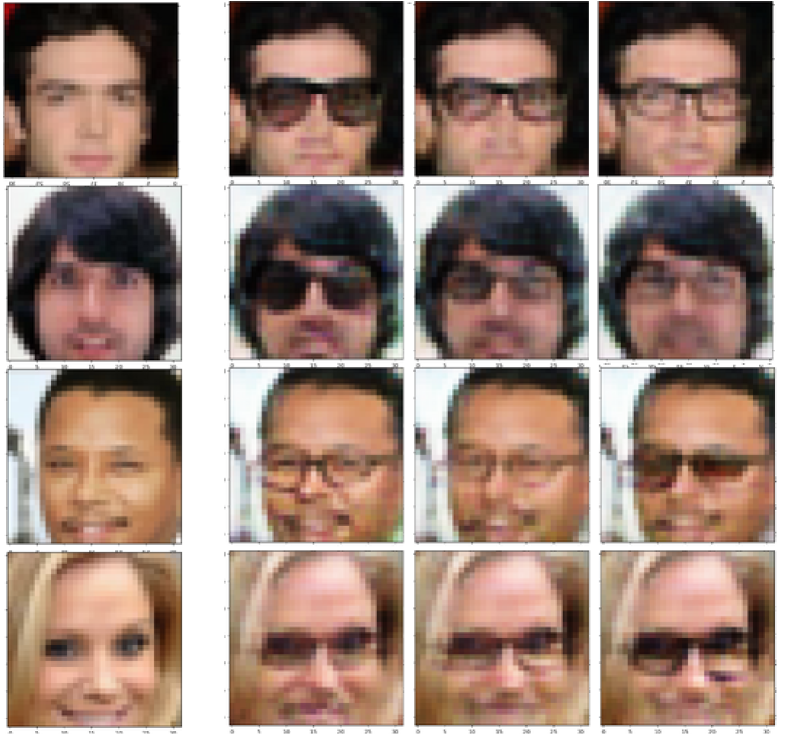
(a)

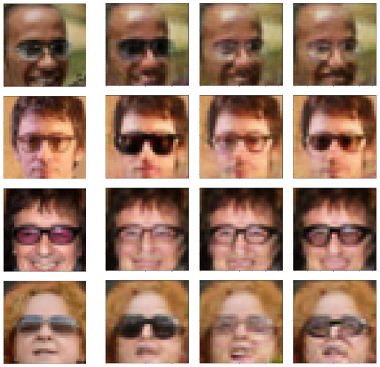
(b)

Figure 5: Parametrically adding glasses (a) and changing glasses (b) on a person’s face. (a): the leftmost column shows a sample from the dataset $a_{i}\in D_{E}(A)$. Three rightmost columns show the result of $c(a_{i},z_{j})$, where $z_{j}\in D_{E}(B_{Z})$ is a randomly sampled latent vector. (b): leftmost column shows a sample from the dataset $(ab)_{i}\in D_{E}(AB)$. Three rightmost columns show the image $c(\pi_{A}(d((ab_{i}))),z_{j})$ which is the result of changing the glasses of a person. The latent vector $z_{j}\in D_{E}(B_{Z})$ is randomly sampled.

In Figure 7 we see the model can learn to remove glasses. Observe how in some cases the model did not learn to remove the glasses properly, as a slight outline of glasses can be seen. An interesting test of the learned semantics can be done by checking if a specific randomly sampled latent vector $z_{j}$ is consistent across different images. Does the resulting image of the application of $g(a_{i},z_{j})$, contain the same glasses as we vary the input image $a_{i}$? The results for the tasks (ii, iii) are shown in Figure 7. It shows how the network has learned to associate a specific vector $z_{j}$ to a specific type of glasses and insert it in a natural way.

We note low diversity in generated glasses and a slight loss in image quality, which is due to suboptimal architecture choice for neural networks. Despite this, these experiments show that it is possible to train networks to (i) remove objects from, and (ii) parametrically insert objects into images in a unsupervised, unpaired fashion. Even though none of the networks were told that images contain people, glasses, or objects of any kind, we highlight that they learned to preserve all the main facial features.

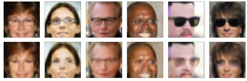
Figure 6: Top row shows samples ${(ab)_{i}\in D_{E}(AB)}$. Bottom row shows the result of a function $\pi_{A}\circ d:AB\rightarrow A$ which removes the glasses from the person.

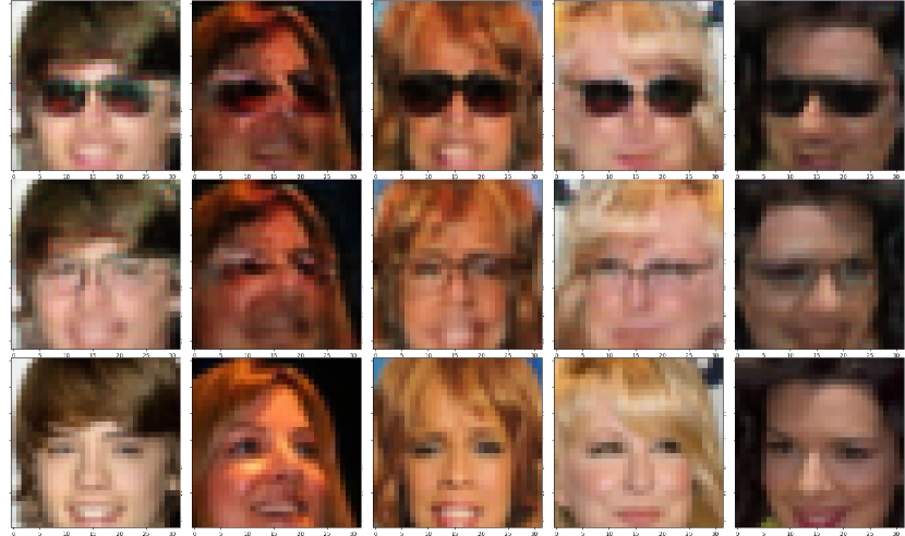
Figure 7: Bottom row shows true samples $a_{i}\in D_{E}(A)$. Top two rows show the image $c(a_{i},z_{j})$ of adding glases with a specific latent vector $z_{1}$ for the topmost row and $z_{2}$ for the middle row. Observe how the general style of the glasses stays the same in a given row, but gets adapted for every person that wears them.

7 From categorical databases to deep learning

The formulation presented in this paper bears a striking and unexpected similarity to Functorial Data Migration (FDM) [14]. Given a categorical schema $\mathbf{Free}(G)/{\sim}$ on some graph $G$, FDM defines a functor category $\mathbf{Set}^{\mathbf{Free}(G)/{\sim}}$ of database instance on that schema. The notion of data integrity is captured by path equivalence relations which ensure any specified “business rules” hold. The analogue of data integrity in neural networks is captured in the same way, first introduced in CycleGAN [16] as cycle-consistency conditions. The main difference between the approaches is that in this paper we do not start out with an implementation of the network instance functor, but rather we randomly initialize it and then learn it.

This shows that the underlying structures used for specifying data semantics for a given database systems are equivalent to the structures used to design data semantics which are possible to capture by training neural networks.

8 Conclusion and future work

In this paper we introduced a categorical formalism for training networks given by an arbitrary categorical schema. We showed there exists a correspondence between categorical formulation of databases and neural network training. We developed a rudimentary theory of learning a specific class of functors using gradient descent. Using the CelebA dataset we obtained experimental results and verified that semantic image manipulation can be carried out in a novel way.

The category theory in this paper is only elementary and we believe there is much more structure to be discovered. This work just scratching the surface of the rich connection between machine learning and category theory. It opens up interesting avenues of research and it seems to be deserving of further exploration.

Appendix A Experiments

In the experiments we have used optimizer Adam [11] and the Wasserstein GAN with gradient penalty [8]. We used the suggested choice of hyperparameters in [8]. The parameter $\gamma$ is set to $20$ and as such weighted the optimization procedure towards the path-equivalence, rather than the cycle-consistency loss. All weights were initialized from a Gaussian distribution $\mathcal{N}(0,0.01)$. As suggested in [8], we always gave the discriminator a head start and trained it more, especially in the beginning. We set $n_{critic}=50$ for the first 50 time steps and $n_{critic}=5$ for all other time steps.

Discriminator $\mathbf{D}(AB)$ and the discriminators for each $A$ and $B$ in $\mathbf{D}(A\times B)$ in first two experiments were $5$-layer ReLU convolutional neural networks of type $\mathbb{R}^{q}\times\mathbb{R}^{32\times 32\times 3}\rightarrow\mathbb{R}$. Kernel size was set to $5$ and padding to $2$. We used stride $2$ to halve image size in all layers except the second, where we used stride $1$. We used a fully-connected layer without any activations at the end of the convolutional network to reduce the output size to $1$.

References

- [1]
- [2] Amjad Almahairi, Sai Rajeswar, Alessandro Sordoni, Philip Bachman & Aaron C. Courville (2018): Augmented CycleGAN: Learning Many-to-Many Mappings from Unpaired Data. CoRR abs/1802.10151. Available at http://arxiv.org/abs/1802.10151.
- [3] Marcin Andrychowicz, Misha Denil, Sergio Gomez Colmenarejo, Matthew W. Hoffman, David Pfau, Tom Schaul & Nando de Freitas (2016): Learning to learn by gradient descent by gradient descent. CoRR abs/1606.04474. Available at http://arxiv.org/abs/1606.04474.
- [4] Martin Arjovsky, Soumith Chintala & Léon Bottou (2017): Wasserstein GAN. arXiv e-prints:arXiv:1701.07875.
- [5] Brendan Fong, David I. Spivak & Rémy Tuyéras (2019): Backprop as Functor: A compositional perspective on supervised learning. In: 34th Annual ACM/IEEE Symposium on Logic in Computer Science, LICS 2019, Vancouver, BC, Canada, June 24-27, 2019, IEEE, pp. 1–13, 10.1109/LICS.2019.8785665.
- [6] Neil Ghani, Jules Hedges, Viktor Winschel & Philipp Zahn (2018): Compositional Game Theory. In Anuj Dawar & Erich Grädel, editors: Proceedings of the 33rd Annual ACM/IEEE Symposium on Logic in Computer Science, LICS 2018, Oxford, UK, July 09-12, 2018, ACM, pp. 472–481, 10.1145/3209108.3209165.
- [7] Ian Goodfellow, Jean Pouget-Abadie, Mehdi Mirza, Bing Xu, David Warde-Farley, Sherjil Ozair, Aaron Courville & Yoshua Bengio (2014): Generative Adversarial Nets. In Z. Ghahramani, M. Welling, C. Cortes, N. D. Lawrence & K. Q. Weinberger, editors: Advances in Neural Information Processing Systems 27, Curran Associates, Inc., pp. 2672–2680. Available at http://papers.nips.cc/paper/5423-generative-adversarial-nets.pdf.
- [8] Ishaan Gulrajani, Faruk Ahmed, Martin Arjovsky, Vincent Dumoulin & Aaron Courville (2017): Improved Training of Wasserstein GANs. arXiv e-prints:arXiv:1704.00028.
- [9] Jules Hedges (2017): On Compositionality. Available at https://julesh.com/2017/04/22/on-compositionality/.
- [10] Max Jaderberg, Wojciech Marian Czarnecki, Simon Osindero, Oriol Vinyals, Alex Graves & Koray Kavukcuoglu (2016): Decoupled Neural Interfaces using Synthetic Gradients. CoRR abs/1608.05343. Available at http://arxiv.org/abs/1608.05343.
- [11] Diederik P. Kingma & Jimmy Ba (2015): Adam: A Method for Stochastic Optimization. In: ICLR.
- [12] Ziwei Liu, Ping Luo, Xiaogang Wang & Xiaoou Tang (2015): Deep Learning Face Attributes in the Wild. In: 2015 IEEE International Conference on Computer Vision, ICCV 2015, Santiago, Chile, December 7-13, 2015, IEEE Computer Society, pp. 3730–3738, 10.1109/ICCV.2015.425.
- [13] Saunders MacLane (1971): Categories for the Working Mathematician. Springer-Verlag, New York. Graduate Texts in Mathematics, Vol. 5.
- [14] David I. Spivak (2012): Functorial data migration. Inf. Comput. 217, pp. 31–51, 10.1016/j.ic.2012.05.001.
- [15] David I. Spivak (2014): Database queries and constraints via lifting problems. Math. Struct. Comput. Sci. 24(6), 10.1017/S0960129513000479.
- [16] Jun-Yan Zhu, Taesung Park, Phillip Isola & Alexei A. Efros (2017): Unpaired Image-to-Image Translation using Cycle-Consistent Adversarial Networks. CoRR abs/1703.10593. Available at http://arxiv.org/abs/1703.10593.