[title=Index] [columns=2, title=Index]

An Introduction to the
Bernoulli Function

Abstract. We explore a variant of the zeta function interpolating the Bernoulli numbers based on an integral representation suggested by J. Jensen. The Bernoulli function $\operatorname{B}(s,v)=-s\,\zeta(1-s,v)$ can be introduced independently of the zeta function if it is based on a formula first given by Jensen in 1895. We examine the functional equation of $\operatorname{B}(s,v)$ and its representation by the Riemann $\zeta$ and $\xi$ function, and recast classical results of Hadamard, Worpitzky, and Hasse in terms of $\operatorname{B}(s,v).$ The extended Bernoulli function defines the Bernoulli numbers for odd indices basing them on rational numbers studied by Euler in 1735 that underlie the Euler and André numbers. The Euler function is introduced as the difference between values of the Hurwitz-Bernoulli function. The André function and the Seki function are the unsigned versions of the extended Euler resp. Bernoulli function.

Notations An Introduction to the Bernoulli Function Index An Introduction to the Bernoulli Function Plots 27 Contents An Introduction to the Bernoulli Function

1 – Prologue: extension by interpolation

The question

André Weil recounts the origin of the gamma function in his historical exposition of number theory [54, p. 275]:

“Ever since his early days in Petersburg Euler had been interested in the interpolation of functions and formulas given at first only for integral values of the argument; that is how he had created the theory of the gamma function.”

The three hundred year success story of Euler’s gamma function shows how fruitful this question is. The usefulness of such an investigation is not limited by the fact that there are infinitely many ways to interpolate a sequence of numbers.

This essay will explore the question: how can the Bernoulli numbers be interpolated most meaningfully?

The method

The Bernoulli numbers had been known for some time at the beginning of the 18th century and used in the (now Euler–Maclaurin called) summation formula in analysis, first without realizing that these numbers are the same each case.

Then, in 1755, Euler baptized these numbers Bernoulli numbers in his Institutiones calculi differentialis (following the lead of de Moivre). After that, things changed, as Sandifer [46] explains:

“… for once the Bernoulli numbers had a name, their diverse occurrences could be recognized, organized, manipulated and understood. Having a name, they made sense.”

The function we are going to talk about is not new. However, it is not treated as a function in its own right and with its own name. So we will give the beast a name. We will call the interpolating function the Bernoulli function. Since, as Mazur [41] asserts, the Bernoulli numbers “act as a unifying force, holding together seemingly disparate fields of mathematics,” this should all the more be manifest in this function.

What to expect

This note is best read as an annotated formula collection; we refer to the cited literature for the proofs.

The Bernoulli function and the Riemann zeta function can be understood as complementary pair. One can derive the properties of one from those of the other. For instance, all the questions Riemann associated with the zeta function can just as easily be discussed with the Bernoulli function. In addition, the introduction of the Bernoulli function leads to a better understanding which numbers the generatingfunctionologists [55] should hang up on their clothesline (see the discussion in [33]).

Seemingly the first to treat the Bernoulli function in our sense was Jensen [25], who gave an integral formula for the Bernoulli function of remarkable simplicity. Except for referencing Cauchy’s theorem, he did not develop the proof. The proof is worked out in Johansson and Blagouchine [28].

A table of contents (An Introduction to the Bernoulli Function) can be found at the end of the paper.

2 – Notations and jump-table to the definitions

$$\operatorname{B}(s,v)\,=\,2\pi\int_{-\infty}^{\infty}\frac{(v-1/2+iz)^{s}}{({\mathrm{e}}^{-\pi z}+{\mathrm{e}}^{\pi z})^{2}}\,dz\hskip 67.0pt\text{Jensen formula}\marginpar{\normalcolor\raggedright$\rightarrow$\underline{\ref{int5}}}\@add@raggedright$$

$$\operatorname{B}(s)\,=\,\operatorname{B}(s,1)\,=\,-s\,\zeta(1-s)\hskip 84.0pt\text{Bernoulli function}\marginpar{\normalcolor\raggedright$\rightarrow$\phantom{8}\underline{\ref{Bdef}}}\@add@raggedright$$

$$\operatorname{B}^{c}(s)\,=\,\operatorname{B}\left(s,1/2\right)\hskip 97.0pt\text{Central Bernoulli function}\marginpar{\normalcolor\raggedright$\rightarrow$\underline{\ref{cbrep}}}\@add@raggedright$$

$$\operatorname{B}^{*}(s)\,=\,\operatorname{B}(s)(1-2^{s})\hskip 70.0pt\text{Alternating Bernoulli function}\marginpar{\normalcolor\raggedright$\rightarrow$\underline{\ref{betastar}}}\@add@raggedright$$

$$\operatorname{B}_{n}\,=\,\operatorname{B}(n)\hskip 171.0pt\text{Bernoulli numbers}\marginpar{\normalcolor\raggedright$\rightarrow$\phantom{8}\underline{\ref{bernum}}}\@add@raggedright$$

$$\operatorname{B}_{\sigma}(s)=\frac{2^{s-1}}{2^{s}-1}\left(\operatorname{B}\left(s,\tfrac{3}{4}\right)-\operatorname{B}\left(s,\tfrac{1}{4}\right)\right)\hskip 22.0pt\text{Bernoulli secant function}\marginpar{\normalcolor\raggedright$\rightarrow$\underline{\ref{bernsec}}}\@add@raggedright$$

$$\operatorname{G}(s,v)\,=\,2^{s}\left(\operatorname{B}\left(s,\tfrac{v}{2}\right)-\operatorname{B}\left(s,\tfrac{v+1}{2}\right)\right)\hskip 28.0pt\text{Gen. Genocchi function}\marginpar{\normalcolor\raggedright$\rightarrow$\underline{\ref{GG}}}\@add@raggedright$$

$$\operatorname{G}(s)\,=\,\operatorname{G}(s,1)\,=\,2(1-2^{s})\operatorname{B}(s)\hskip 69.0pt\text{Genocchi function}\marginpar{\normalcolor\raggedright$\rightarrow$\underline{\ref{GenocciFun2}}}\@add@raggedright$$

$$\operatorname{E}(s,v)\,=\,-\frac{\operatorname{G}(s+1,v)}{s+1}\hskip 73.0pt\text{Generalized Euler function}\marginpar{\normalcolor\raggedright$\rightarrow$\underline{\ref{EG}}}\@add@raggedright$$

$$\operatorname{E}_{\tau}(s)\,=\,\operatorname{E}(s,1)\hskip 129.0pt\text{Euler tangent function}\marginpar{\normalcolor\raggedright$\rightarrow$\underline{\ref{eulsimpl}}}\@add@raggedright$$

$$\operatorname{E}_{\sigma}(s)\,=\,2^{s}\operatorname{E}(s,\tfrac{1}{2})\hskip 122.0pt\text{Euler secant function}\marginpar{\normalcolor\raggedright$\rightarrow$\underline{\ref{EulerCentral}}}\@add@raggedright$$

$$\operatorname{E}_{n}\,=\,\operatorname{E}_{\sigma}(n)\hskip 184.0pt\text{Euler numbers}\marginpar{\normalcolor\raggedright$\rightarrow$\underline{\ref{EulerNum}}}\@add@raggedright$$

$$\widetilde{\zeta}(s)\,=\,\zeta\left({s}\right)+\frac{\zeta\left({s},{\frac{1}{4}}\right)-\zeta\left({s},{\frac{3}{4}}\right)}{2^{s}-2}\hskip 52.0pt\text{Extended zeta function}\marginpar{\normalcolor\raggedright$\rightarrow$\underline{\ref{lzeta}}}\@add@raggedright$$

$$\mathcal{B}(s)\,=\,-s\,\widetilde{\zeta}(1-s)\hskip 91.0pt\text{Extended Bernoulli function}\marginpar{\normalcolor\raggedright$\rightarrow$\underline{\ref{genbern}}}\@add@raggedright$$

$$\mathcal{E}(s)\,=\,\frac{4^{s+1}-2^{s+1}}{(s+1)!}\mathcal{B}(s+1)\hskip 66.0pt\text{Extended Euler function}\marginpar{\normalcolor\raggedright$\rightarrow$\underline{\ref{exteulbern}}}\@add@raggedright$$

$$\mathcal{A}(s)\,=\,(-i)^{s+1}\operatorname{Li}_{-s}(i)\,+\,i^{s+1}\operatorname{Li}_{-s}(-i)\hskip 56.0pt\text{Andr\'{e} function}\marginpar{\normalcolor\raggedright$\rightarrow$\underline{\ref{UnsignedAndreFun}}}\@add@raggedright$$

$$\mathcal{A}^{\ast}(s)\,=\,ie^{-\frac{1}{2}i\pi s}\left(\text{Li}_{-s}(-i)-e^{i\pi s}\text{Li}_{-s}(i)\right)\hskip 7.0pt\text{Signed Andr\'{e} function}\marginpar{\normalcolor\raggedright$\rightarrow$\underline{\ref{SignedAndreFun}}}\@add@raggedright$$

$$\mathcal{S}(s)\,=\frac{s\,\mathcal{A}(s-1)}{4^{s}-2^{s}}\hskip 162.0pt\text{Seki function}\marginpar{\normalcolor\raggedright$\rightarrow$\underline{\ref{SekiAndreFun}}}\@add@raggedright$$

$$\mathcal{S}^{\ast}(s)\,=\,\frac{s\,e^{i\pi s/2}}{2^{s}-4^{s}}\left(e^{i\pi s}\text{Li}_{1-s}(-i)+\text{Li}_{1-s}(i)\right)\hskip 8.0pt\text{Signed Seki function}\marginpar{\normalcolor\raggedright$\rightarrow$\underline{\ref{SignedSekiFun}}}\@add@raggedright$$

$$\mathcal{Z}_{n}\,=\,\frac{\mathcal{A}_{n}}{n!}\hskip 172.0pt\text{Euler zeta numbers}\marginpar{\normalcolor\raggedright$\rightarrow$\underline{\ref{eulzetanum}}}\@add@raggedright$$

$$\operatorname{\xi}(s)\,=\,\operatorname{B}(s)\,\frac{\sigma!}{\pi^{\sigma}}\ \text{with }\sigma=(1-s)/2\hskip 54.0pt\text{Riemann }\xi\text{ function}\marginpar{\normalcolor\raggedright$\rightarrow$\underline{\ref{q554}}}\@add@raggedright$$

$$\gamma\,=\,-\operatorname{B}^{{}^{\prime}}(0)\ \text{(Euler),}\quad\gamma_{n-1}\,=\,-\frac{1}{n}\operatorname{B}^{(n)}(0)\quad\hskip 11.0pt\text{Stieltjes constants}\marginpar{\normalcolor\raggedright$\rightarrow$\underline{\ref{q26}}}\@add@raggedright$$

​

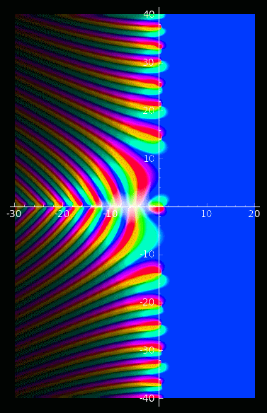
Figure 1: The zeta and the Bernoulli function in the complex plane.

3 – Stieltjes constants and Zeta function

The generalized Euler constants, also called Stieltjes constants, are the real numbers $\gamma_{n}$ defined by the Laurent series in a neighborhood of $s=1$ of the Riemann zeta function ([1, 45]),

$$\zeta(s)=\frac{1}{s-1}+\sum_{n=0}^{\infty}\frac{(-1)^{n}}{n!}\gamma_{n}(s-1)^{n},\qquad(s\neq 1).$$ (1)

As a particular case they include the Euler constant $\gamma_{0}=\gamma\ \,(\approx\frac{228}{395})$. Blagouchine [7] gives a detailed discussion with many historical notes. Following Franel [17], Blagouchine [6] shows that

$$\gamma_{n}\,=\,-\frac{2\,\pi}{n+1}\int\limits_{-\infty}^{+\infty}\,\frac{\log\!\left(\frac{1}{2}+iz\right)^{n+1}}{\left({{\mathrm{e}}^{-\pi\,z}}+{{\mathrm{e}}^{\pi\,z}}\right)^{2}}\,{dz}.$$ (2)

Here, and in all later similar formulas, we write $f(x)^{n}$ for $(f(x))^{n}$ and take the principal branch of the logarithm implicit in the exponential.

Recently Johansson [26] observed that one can employ the integral representation (2) in a particularly efficient way to approximate the Stieltjes constants with prescribed precision numerically.

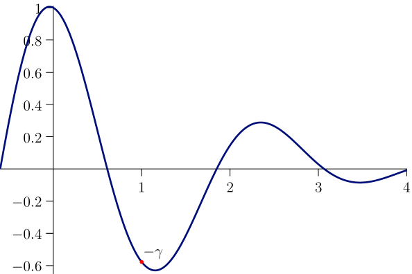
Figure 2: The Bernoulli constants seen as values of a real function.

4 – Bernoulli constants and Bernoulli function

The Bernoulli constants $\beta_{n}$ are defined for $n\geq 0$ as

$${\beta_{n}\,=\,2\pi\!\int\limits_{-\infty}^{+\infty}{\frac{\log\!\left(\frac{1}{2}+iz\right)^{n}}{\left({{\mathrm{e}}^{-\pi\,z}}+{{\mathrm{e}}^{\pi\,z}}\right)^{2}}}\,{dz}.}$$ (3)

The Bernoulli function is defined as

$$\operatorname{B}(s)\,=\,\sum_{n=0}^{\infty}\beta_{n}\frac{s^{n}}{n!}\,.$$ (4)

Since $\beta_{0}=1$ we have in particular $\operatorname{B}(0)=1$.

Comparing the definitions of the constants $\gamma_{n}$ and $\beta_{n}$, we see that in (3) the exponent of the power is synchronous to the index and the factor $-1/(n+1)$ in (2) has disappeared. In other words, $\gamma_{n}=-\frac{\beta_{n+1}}{n+1}$, and the Riemann zeta representation of the Bernoulli function becomes

$$\operatorname{B}(s) =\sum_{n=0}^{\infty}\beta_{n}\frac{s^{n}}{n!}$$

$$=1+\sum_{n=1}^{\infty}\beta_{n}\frac{s^{n}}{n!}$$

$$=1+\sum_{n=0}^{\infty}\beta_{n+1}\frac{s^{n+1}}{(n+1)!}$$

$$=1-\sum_{n=0}^{\infty}\gamma_{n}\frac{s^{n+1}}{n!}$$

$$=1-s\sum_{n=0}^{\infty}\gamma_{n}\frac{s^{n}}{n!}$$

$$=-s\zeta(1-s).$$ (5)

The singularity of $-s\zeta(1-s)$ at $s=0$ is removed by $\operatorname{B}(0)=1$. Thus $\operatorname{B}(s)$ is an entire function with its defining series converging everywhere in $\mathbb{C}$.

5 – The Bernoulli numbers

We define the Bernoulli numbers as the values of the Bernoulli function at the nonnegative integers. According to (4) this means

$$\operatorname{B}_{n}\,=\,\operatorname{B}(n)\,=\,\sum_{j=0}^{\infty}\beta_{j}\frac{n^{j}}{j!}.$$ (6)

Since for $n>1$ an odd integer $-n\zeta(1-n)=0$, the Bernoulli numbers vanish at these integers and $\operatorname{B}_{n}=1-n\sum_{j=0}^{\infty}\gamma_{j}\frac{n^{j}}{j!}$ implies

$$\sum_{j=0}^{\infty}\gamma_{j}\frac{n^{j}}{j!}=\frac{1}{n}\text{ and }\sum_{j=0}^{\infty}\beta_{j}\frac{n^{j}}{j!}=0\qquad(n>1\text{ odd}).$$ (7)

6 – The expansion of the Bernoulli function

The Bernoulli function $\operatorname{B}(s)=-s\zeta(1-s)$ can be expanded by using the generalized Euler–Stieltjes constants

$$\operatorname{B}(s)\,=\,1-\gamma s-\gamma_{1}s^{2}-\frac{\gamma_{2}}{2}s^{3}-\frac{\gamma_{3}}{6}s^{4}\,\ldots\ .$$ (8)

Or, in its natural form, using the Bernoulli constants

$${\operatorname{B}(s)\,=\,1+\beta_{1}s+\frac{\beta_{2}}{2}s^{2}+\frac{\beta_{3}}{6}s^{3}+\frac{\beta_{4}}{24}s^{4}\,\ldots\ .}$$ (9)

$r$	$\beta(r)\quad\qquad\qquad\qquad\qquad\qquad$
$-1$	-1.0967919991262275651322398023421657187190$\dots$
$-1/2$	0.3000952439768656513643742483305378454480$\dots$
$0$	1.0
$1/2$	0.2364079388130323148951169845913737350793$\dots$
$1$	-0.5772156649015328606065120900824024310421$\dots$
$3/2$	-0.4131520868458801199329318166967102536980$\dots$
$2$	0.1456316909673534497211727517498026382754$\dots$
$5/2$	0.2654200629584708272795102903586382709016$\dots$
$3$	0.0290710895786169554535911581056375880771$\dots$
$7/2$	-0.0845272473711484887663180676975841853310$\dots$
$4$	-0.0082153376812133834646401861710135371428$\dots$

Table 1: The Bernoulli constants for some rational $r$.

Although we will often refer to the well-known properties of the zeta function when using (5), our definition of the Bernoulli function and the Bernoulli numbers only depends on (3) and (4).

The index $n$ in definition (3) is not restricted to integer values. For illustration the function $\beta_{r}$ is plotted in figure 2, where the index $r$ of $\beta$ is understood to be a real number. The table above displays some numerical values of Bernoulli constants.

7 – Integral formulas for the Bernoulli constants

Let us come back to the definition of $\beta_{n}$ as given in (3). The appearance of the imaginary unit forces complex integration; on the other hand, only the real part of the result is used. Fortunately, the definition can be simplified such that the computation stays in the realm of reals provided $n$ is a nonnegative integer.

Using the symmetry of the integrand with respect to the $y$-axis and $\left({{\mathrm{e}}^{-\pi\,z}}+{{\mathrm{e}}^{\pi\,z}}\right)^{2}=4\cosh(\pi z)^{2}$ we get from the definition (3)

$$\beta_{n}\ =\ \pi\!\int_{0}^{\infty}\,{\frac{\mathop{\rm Re}\nolimits\!\left(\log(\frac{1}{2}+iz)^{n}\right)}{\cosh(\pi z)^{2}}}dz\,.$$ (10)

For the numerator of the integrand we set for $n\geq 0$

$$\sigma_{n}(z)\,=\,\mathop{\rm Re}\nolimits(\log(\tfrac{1}{2}+iz)^{n}).$$ (11)

By induction we see that

$$\sigma_{n}(z)=\sum_{k=0}^{\lfloor n/2\rfloor}(-1)^{k}\binom{n}{2k}a(z)^{n-2k}\,b(z)^{2k},$$ (12)

where $a(z)=\log(z^{2}+\frac{1}{4})/2$ and $b(z)=\arctan(2z)$.

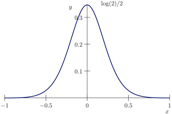
Figure 3: $f(z)=-\log((z^{2}+\frac{1}{4})^{\frac{1}{4}})\operatorname{sech}(\pi z)^{2}$ with $\int_{-\infty}^{\infty}f(z)\,dz=\frac{\gamma}{\pi}.$

Therefore the constants can be computed by real integrals,

$$\beta_{n}\,=\,\pi\!\int_{0}^{\infty}\frac{\sigma_{n}(z)}{\cosh(\pi z)^{2}}\,dz\,.$$ (13)

Similarly we have for the Stieltjes constants

$$\gamma_{n}\,=\,-\frac{\pi}{n+1}\int_{0}^{\infty}\frac{\sigma_{n+1}(z)}{\cosh(\pi z)^{2}}\,dz\,.$$ (14)

8 – Some special integral formulas

Let us consider some special cases of these integral formulas. Formula (14) reads for $n=0$

$$\gamma\,=\,-\pi\int_{0}^{\infty}\frac{\log(z^{2}+\tfrac{1}{4})}{2\cosh(\pi z)^{2}}\,dz.$$ (15)

This follows since for real $z$

$$\sigma_{1}(z)=\mathop{\rm Re}\nolimits\log\left(\frac{1}{2}+iz\right)=\log\left(\frac{1}{2}\sqrt{4z^{2}+1}\right)=\frac{1}{2}\log\left(z^{2}+\frac{1}{4}\right).$$

Using the symmetry of the integrand with respect to the $y$-axis this can be rephrased as: Euler’s gamma is $\pi$ times the integral of $-\log((z^{2}+\tfrac{1}{4})^{\tfrac{1}{4}})\operatorname{sech}(\pi z)^{2}$ over the real line. See figure 3.

With the abbreviations $a=\log(z^{2}+\frac{1}{4})/2,\,b=\arctan(2z)$ and $c=\cosh(\pi z)$ the first few Bernoulli constants are by (12):

$$\beta_{1}\, =\,\pi\int_{0}^{\infty}\frac{a}{c^{2}}\,dz\,,$$ (16)

$$\beta_{2}\, =\,\pi\int_{0}^{\infty}\frac{a^{2}-b^{2}}{c^{2}}\,dz\,,$$ (17)

$$\beta_{3}\, =\,\pi\int_{0}^{\infty}\frac{a^{3}-3ab^{2}}{c^{2}}\,dz\,,$$ (18)

$$\beta_{4}\, =\,\pi\int_{0}^{\infty}\frac{a^{4}-6a^{2}b^{2}+b^{4}}{c^{2}}\,dz\,,$$ (19)

$$\beta_{5}\, =\,\pi\int_{0}^{\infty}\frac{a^{5}-10a^{3}b^{2}+5ab^{4}}{c^{2}}\,dz\,.$$ (20)

9 – Generalized Bernoulli constants

We recall that $\gamma_{n}/n!$ is the coefficient of $(1-s)^{n}$ in the Laurent expansion of $\zeta(s)$ about $s=1$ and $\gamma_{n}(v)/n!$ is the coefficient of $(1-s)^{n}$ in the Laurent expansion of $\zeta(s,v)$ about $s=1$. In other words, with the generalized Stieltjes constants $\gamma_{n}(v)$ we have the Hurwitz zeta function $\zeta(s,v)$ in the form

$$\zeta(s,v)=\frac{1}{s-1}+\sum_{n=0}^{\infty}\frac{(-1)^{n}}{n!}\gamma_{n}(v)(s-1)^{n},\quad(s\neq 1).$$ (21)

The generalized Stieltjes constants may be computed for $n\geq 0$ and $\mathop{\rm Re}\nolimits(v)>\frac{1}{2}$ by an extension of the integral representation (2), see Johansson and Blagouchine [28, formulas 2, 32, 42].

$$\gamma_{n}(v)\,=\,-\frac{\pi}{2(n+1)}\int_{-\infty}^{\infty}\frac{\log\!\left(v-\tfrac{1}{2}+iz\right)^{n+1}}{\cosh(\pi x)^{2}}\,dz.$$ (22)

The generalized Bernoulli constants are defined as

$${\beta_{s}(v)=2\pi\!\int_{-\infty}^{+\infty}\!\frac{\,\log\!\big{(}v-\frac{1}{2}+ix\big{)}^{s}\,}{\left({\mathrm{e}}^{-\pi x}+{\mathrm{e}}^{\pi x}\right)^{2}}\,dx.}$$ (23)

We see that $\beta_{0}(v)=1$ for all $v$ and $\beta_{n}(v)=-n\gamma_{n-1}(v)$ for $n\geq 1$.

10 – The generalized Bernoulli function

We introduce the generalized Bernoulli function $\operatorname{B}(s,v)$ analogous to the Hurwitz zeta function. The new parameter $v$ can be any complex number that is not a nonpositive integer. Then we define the generalized Bernoulli function as

$${\operatorname{B}(s,v)\,=\,\sum_{n=0}^{\infty}\beta_{n}(v)\frac{s^{n}}{n!}\,.}$$ (24)

For $v=1,$ this is the ordinary Bernoulli function (4). Using the identities from the last section, we get

$$\operatorname{B}(s,v)=1-s\sum_{n=0}^{\infty}\gamma_{n}(v)\frac{s^{n}}{n!}.$$ (25)

Thus the generalized Bernoulli function can be represented by

$$\operatorname{B}(s,v)=-s\,\zeta(1-s,v),\qquad(s\neq 1).$$ (26)

This identity also embeds the Bernoulli polynomials as

$$\operatorname{B}_{n}(x)\,=\,\operatorname{B}(n,x)\quad(n\geq 0,n\text{ integer}).$$ (27)

This follows from (26) (see for instance Apostol [4, th. 12.13]) and the fact that $\operatorname{B}(0,x)\,=\,1.$

11 – Integral formulas for the Bernoulli function

We can transfer the integral formulas for the Bernoulli constants to the Bernoulli function itself. First we reproduce a formula by Jensen [25], which he gave in reply to Cesàro in L’Intermédiaire des mathématiciens.

$${(s-1)\zeta(s)\,=\,2\pi\int_{-\infty}^{\infty}\frac{(\tfrac{1}{2}+iy)^{1-s}}{({\mathrm{e}}^{\pi y}+{\mathrm{e}}^{-\pi y})^{2}}\,dy.}$$ (28)

Jensen comments:

“… [this formula] is remarkable because of its simplicity and can easily be demonstrated with the help of Cauchy’s theorem.”

How Jensen actually computed $(s-1)\zeta(s)$ is unclear, since the formula for the coefficients $\operatorname{c}_{v}$, which he states, rapidly diverges. This was observed by Kotěšovec (personal communication).

In a numerical example Jensen uses the Bernoulli constants in the form $\operatorname{c}_{v}\,=\,(-1)^{v}\beta_{v}/{v!}.$ Applied to the Bernoulli function, Jensen’s formula is written as

$${\operatorname{B}(s)\,=\,2\pi\int_{-\infty}^{\infty}\frac{(\tfrac{1}{2}+iz)^{s}}{({\mathrm{e}}^{\pi z}+{\mathrm{e}}^{-\pi z})^{2}}\,dz.}$$ (29)

In Johansson and Blagouchine [28] this is a particular case of the first formula of theorem 1. (See also Srivastava and Choi [50, p. 92] and the discussion [49].)

Hadjicostas [20] remarks that from this theorem also the representation for the generalized Bernoulli function follows:

For all $s\in\mathbb{C}$ and $v\in\mathbb{C}$ with $\mathop{\rm Re}\nolimits(v)\geq 1/2$

$${\operatorname{B}(s,v)\,=\,2\pi\int_{-\infty}^{\infty}\frac{(v-\tfrac{1}{2}+iz)^{s}}{({\mathrm{e}}^{\pi z}+{\mathrm{e}}^{-\pi z})^{2}}\,dz.}$$ (30)

This formula is the central formula in this paper.

Figure 4: The Hurwitz Bernoulli functions with $s=2+k/6,$
$(0\leq k\leq 6),$ deform $\operatorname{B}_{2}(x)$ into $\operatorname{B}_{3}(x).$

12 – The Hurwitz–Bernoulli function

The Hurwitz–Bernoulli function is defined as

$$\begin{split}\operatorname{H}(s,v)&={\mathrm{e}}^{-i\pi s/2}\,\operatorname{L}(s,v)+{\mathrm{e}}^{i\pi s/2}\,\operatorname{L}(s,1-v),\\ \operatorname{L}(s,v)&=-\frac{s\,!}{(2\pi)^{s}}\operatorname{Li}_{s}({\mathrm{e}}^{2\pi iv}).\end{split}$$ (31)

Here $\operatorname{Li}_{s}(v)$ denotes the polylogarithm. The proposition that

$$\operatorname{B}_{s}(v)=\operatorname{B}(s,v)=\operatorname{H}(s,v),\ \ \text{for }0\leq v\leq 1\text{ and }s>1,$$ (32)

goes back to Hurwitz. The corresponding case for the zeta function (32) is known as the Hurwitz formula [4, p. 71]. With the Hurwitz–Bernoulli function the Bernoulli polynomials can be continuously deformed into each other (see figure 4).

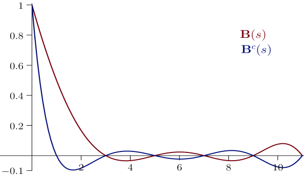
Figure 5: The Bernoulli function and the central Bernoulli function

13 – The central Bernoulli function

Setting $v=1$ in (32) the Hurwitz–Bernoulli function simplifies to

$${\operatorname{B}_{s}(1)\,=\,-2\,s!\operatorname{Li}_{s}(1)\cos(s\pi/2)/(2\pi)^{s},\quad(s>1).}$$ (33)

For $s>1$ one can replace the polylogarithm with the zeta function and then apply the functional equation of the zeta function to get

$$\operatorname{B}_{s}(1)\,=\,-s\zeta(1-s),\qquad(s>1).$$ (34)

Thus the Bernoulli function is a vertical section of the Hurwitz–Bernoulli function, $\operatorname{B}(s)=\operatorname{B}_{s}(1),$ similarly as the Bernoulli numbers are special cases of the Bernoulli polynomials, $\operatorname{B}_{n}=\operatorname{B}_{n}(1)$.

Setting $v=1/2$ in the Hurwitz–Bernoulli function leads to a second noteworthy case. Then (32) reduces to

$${\operatorname{B}_{s}(1/2)\,=\,-2\,s!\operatorname{Li}_{s}(-1)\cos(s\pi/2)/(2\pi)^{s},\quad(s>1).}$$ (35)

For $s>1$ we can replace the polylogarithm with the negated alternating zeta function. We call $\operatorname{B}^{c}(s)=\operatorname{B}_{s}(1/2)$ the central Bernoulli function.

The function can be expressed as $\operatorname{B}^{c}(s)=-s\zeta(1-s)(2^{1-s}-1)$ for $s>1$, or by the Bernoulli function as

$$\operatorname{B}^{c}(s)=\operatorname{B}(s)(2^{1-s}-1).$$ (36)

The central Bernoulli function has the same trivial zeros as the Bernoulli function, plus a zero at the point $s=1$ (see figure 5).

An integral representation for the central Bernoulli function follows from (30). For all $s\in\mathbb{C}$

$${\operatorname{B}^{c}(s)\,=\,2\pi\int_{-\infty}^{\infty}\frac{(iz)^{s}}{({\mathrm{e}}^{-\pi z}+{\mathrm{e}}^{\pi z})^{2}}\,dz.}$$ (37)

Assuming $s>0$ and real, it follows from (36) and (37) that

$${\operatorname{B}(s)\,=\,\pi\,\frac{\cos(\pi s/2)}{2^{1-s}-1}\int_{0}^{\infty}z^{s}\operatorname{sech}(\pi z)^{2}\,dz.}$$ (38)

For $s=1$ the value on the right-hand side of (38) is to be understood as the limit value $(\pi^{2}/\log(4))(\log(2)/\pi^{2})=1/2$.

We call (38) the secant decomposition of $\operatorname{B}(s)$ (see figure 6).

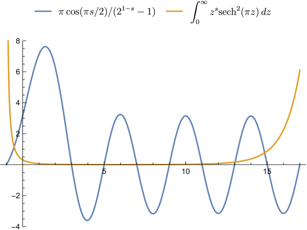
Figure 6: The secant decomposition of the real Bernoulli function.

14 – The central Bernoulli polynomials

The central Bernoulli numbers are defined as

$$\operatorname{B}^{c}_{n}=2^{n}\operatorname{B}_{n}(1/2).$$ (39)

The first few are, for $n\geq 0$:

$$1,\,0,\,-\frac{1}{3},\,0,\,\frac{7}{15},\,0,\,-\frac{31}{21},\,0,\,\frac{127}{15},\,0,\,-\frac{2555}{33},\,0,\frac{1414477}{1365},\ldots.$$

$\phantom{-}1$
$\phantom{-}x$
$-{\frac{1}{3}}\,+\,{x}^{2}$
$-{x}\,+\,{x}^{3}$
$\phantom{-}{\frac{7}{15}}\,-\,{2\,{x}^{2}}\,+\,{x}^{4}$
$\phantom{-}{\frac{7}{3}\,x}\,-\,{\frac{10}{3}\,{x}^{3}}\,+\,{x}^{5}$
$-{\frac{31}{21}}\,+\,{7\,{x}^{2}}\,-\,5\,{x}^{4}\,+\,{x}^{6}$
$-{\frac{31}{3}\,x}\,+\,{\frac{49}{3}\,{x}^{3}}\,-\,7\,{x}^{5}\,+\,{x}^{7}$
${\frac{127}{15}}-{\frac{124}{3}\,{x}^{2}}+{\frac{98}{3}\,{x}^{4}}-{\frac{28}{3}\,{x}^{6}}+{x}^{8}$
${\frac{381}{5}\,x}-124\,{x}^{3}+{\frac{294}{5}\,{x}^{5}}-12\,{x}^{7}+{x}^{9}$

Table 2: The central Bernoulli polynomials $\operatorname{B}_{n}^{c}(x)$.

Unsurprisingly Euler, in 1755 in his Institutiones, also calculated some central Bernoulli numbers, B(3,1) and B(5,1) (Opera Omnia, Ser. 1, Vol. 10, p. 351).

The central Bernoulli polynomials are by definition the Appell sequence

$$\operatorname{B}_{n}^{c}(x)\,=\,\sum_{k=0}^{n}\binom{n}{k}\operatorname{B}^{c}_{k}x^{n-k}.$$ (40)

The parity of $n$ equals the parity of $\operatorname{B}_{n}^{c}(x),$ a property the Bernoulli polynomials do not possess.

Despite their systematic significance, the central Bernoulli polynomials were not in the OEIS database at the time of writing these lines (now they are filed in OEIS A335953).

Also the following identity is worth noting:

$$2^{n}\operatorname{B}_{n}(1)\,=\,\sum_{k=0}^{n}\binom{n}{k}2^{k}\operatorname{B}_{k}\left(\tfrac{1}{2}\right).$$ (41)

We will come back to this identity later, as it highlights the correct choice of the generating function of the Bernoulli numbers.

$0$
$-1$
$1-2x$
$3x-3x^{2}$
$-1+6x^{2}-4x^{3}$
$-5x+10x^{3}-5x^{4}$
$3-15x^{2}+15x^{4}-6x^{5}$
$21x-35x^{3}+21x^{5}-7x^{6}$
$-17+84x^{2}-70x^{4}+28x^{6}-8x^{7}$

Table 3: The Genocchi polynomials $\operatorname{G}_{n}(x)$.

15 – The Genocchi function

How much does the central Bernoulli function deviate from the Bernoulli function? The Genocchi function answers this question (up to a normalization factor).

$$\operatorname{G}(s)\,=\,2^{s}\left(\operatorname{B}^{c}(s)-\operatorname{B}(s)\right)=\,2^{s}\left(\operatorname{B}_{s}(\tfrac{1}{2})-\operatorname{B}_{s}(1)\right).$$ (42)

From the identities (34) and (36), it follows that the Genocchi function can be represented as

$$\operatorname{G}(s)\,=\,2(1-2^{s})\operatorname{B}(s).$$ (43)

The Genocchi function takes integer values for nonnegative integer arguments. The Genocchi numbers $\operatorname{G}_{n}=\operatorname{G}(n)$ are listed in OEIS A226158. The correct sign of $\operatorname{G}_{1}=-1$ must be observed.

$$\operatorname{G}_{n}=0,\,-1,\,-1,\,0,\,1,\,0,\,-3,\,0,\,17,\,0,\,-155,\,0,\,2073,\,\dots$$

The generalized Genocchi function generalizes the definition (42),

$$\operatorname{G}(s,v)\,=\,2^{s}\left(\operatorname{B}\left(s,\frac{v}{2}\right)-\operatorname{B}\left(s,\frac{v+1}{2}\right)\right).$$ (44)

The plain Genocchi function is recovered by $\operatorname{G}(s)=\operatorname{G}(s,1)$.

For $n$ integer (44) gives the Genocchi polynomials

$${\operatorname{G}_{n}(x)=\,2^{n}\left(\operatorname{B}_{n}\left(\frac{x}{2}\right)-\operatorname{B}_{n}\left(\frac{x+1}{2}\right)\right).}$$ (45)

The Genocchi polynomials are twice the difference between the Bernoulli polynomials and the central Bernoulli polynomials.

$${\operatorname{G}_{n}(x)=\,2\left(\operatorname{B}_{n}(x)-\operatorname{B}^{c}_{n}(x)\right).}$$ (46)

The integer coefficients of these polynomials (with different signs) are A333303 in the OEIS . The Genocchi function is closely related to the alternating Bernoulli function, as we will see next.

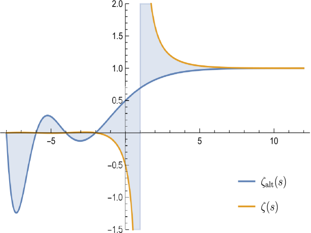
Figure 7: Riemann zeta versus Riemann alternating zeta.

16 – The alternating Bernoulli function

The alternating Riemann zeta function, also known as the Dirichlet eta function, is defined as

$$\zeta^{*}(s)=(1-2^{1-s})\zeta(s),\quad(s\neq 1).$$ (47)

The alternating Bernoulli function is defined in analogy to the representation of the Bernoulli function by the zeta function.

$$\operatorname{B}^{*}(s)=-s\zeta^{*}(1-s),\qquad(s\neq 0).$$ (48)

The alternating Hurwitz zeta function is set for $0<x\leq 1$ as

$$\zeta^{*}(s,x)\,=\,\sum_{n=0}^{\infty}\frac{(-1)^{n}}{(n+x)^{s}},\quad\text{for }\mathop{\rm Re}\nolimits(s)>0,$$ (49)

and for other values by analytic continuation. This function is represented by the Hurwitz Zeta function as

$$\zeta^{*}(s,x)\,=\,2^{-s}\left(\zeta\left(s,\frac{x}{2}\right)-\zeta\left(s,\frac{x+1}{2}\right)\right),\quad(s\neq 1).$$ (50)

The alternating Bernoulli polynomials are defined as

$$\operatorname{B}^{*}_{n}(x)\,=\,-n\zeta^{*}(1-n,x)\,.$$ (51)

This definition is in analogy to the introduction of the Bernoulli polynomials (27).

The alternating Bernoulli function can be represented by the Bernoulli function

$$\operatorname{B}^{*}(s)=\left(1-2^{s}\right)\operatorname{B}(s).$$ (52)

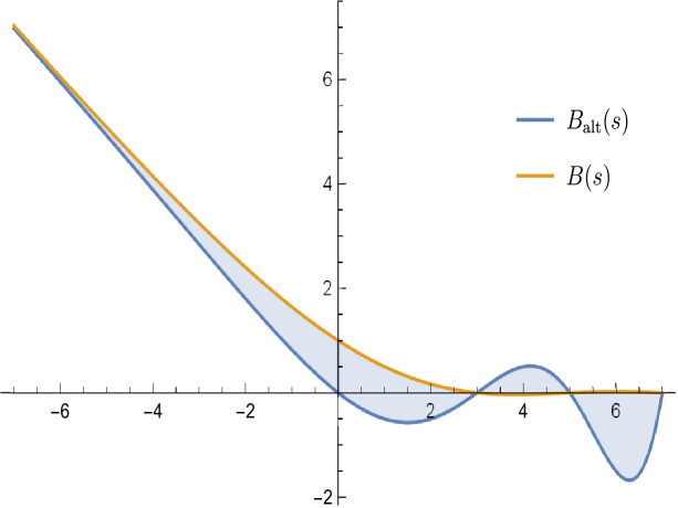
Figure 8: Bernoulli function versus Bernoulli alternating function.

The alternating Bernoulli numbers $\operatorname{B}^{*}_{n}=\operatorname{B}^{*}(n)$ are the values of the alternating Bernoulli function at the nonnegative integers, and are, like the Bernoulli numbers, rational numbers.

Reduced to lowest terms, they have the denominator $2$ and by (45) are half the Genocchi numbers.

$$\operatorname{B}^{*}_{n}\,=\,2^{n-1}\left(\operatorname{B}_{n}\left(\frac{1}{2}\right)-\operatorname{B}_{n}\left(1\right)\right)=\operatorname{G}_{n}/2.$$ (53)

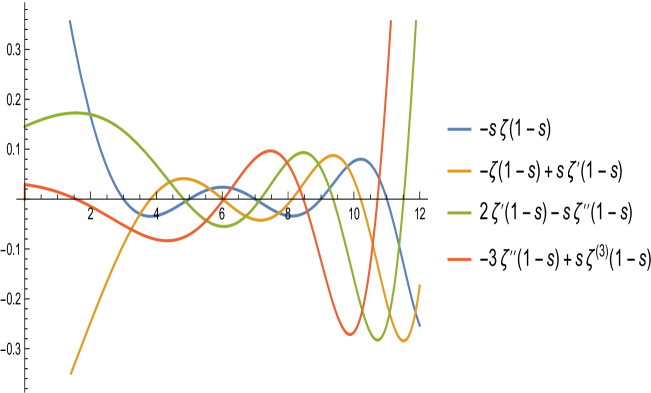
Figure 9: The derivatives of the Bernoulli function $\operatorname{B}^{(n)}(s),\,0\leq n\leq 3.$

17 – Derivatives of the Bernoulli function

The Bernoulli constants are in a simple relationship with the derivatives of the Bernoulli function. With the Riemann zeta function we have

$${\operatorname{B}^{(n)}(s)=(-1)^{n}\left(n\zeta^{(n-1)}(1-s)-s\zeta^{(n)}(1-s)\right).}$$ (54)

Here $\operatorname{B}^{(n)}(s)$ denotes the $n$-th derivative of the Bernoulli function.

Taking $\lim_{s\rightarrow 0}$ on the right hand side of (54) we get

$$\operatorname{B}^{(n)}(0)=\beta_{n}=-n\,\gamma_{n-1}\quad(n\geq 1)\,.$$ (55)

Entire books [22] have been written about the emergence of Euler’s gamma in number theory. The identity ${-\operatorname{B}^{\prime}(0)=\gamma}$ is one of the beautiful places where this manifests (see figure 9).

Figure 10: $-\operatorname{B}^{\prime}(x)$ hits Euler’s $\gamma$ at $x=0,$ dots are Bernoulli numbers.

18 – Logarithmic derivative and Bernoulli cumulants

The logarithmic derivative of a function $\operatorname{F}$ will be denoted by

$$\mathcal{L}\!\operatorname{F}(s)=\frac{\operatorname{F}^{\prime}(s)}{\operatorname{F}(s)}.$$

In particular we will write $\mathcal{L}\!\operatorname{B}(s),\,\mathcal{L}\zeta(s)$, and $\mathcal{L}\Gamma(s)$ for the logarithmic derivative of the Bernoulli function, the $\zeta$ function, and the $\Gamma$ function. $\mathcal{L}\Gamma(s)$ is also known as the digamma function $\psi$.

In terms of the zeta function $\mathcal{L}\!\operatorname{B}(s)$ can also be written

$$\mathcal{L}\!\operatorname{B}(s)\,=\,\frac{1}{s}-\mathcal{L}\zeta(1-s).$$ (56)

If $s=0$ then $\mathcal{L}\!\operatorname{B}(0)$ is set to the limiting value $-\gamma$. For odd integer $n=3,5,7,\ldots$ the value of $\mathcal{L}\!\operatorname{B}(n)$ is undefined.

From (56) we can infer

$${\mathcal{L}\!\operatorname{B}(s)\,=\,\mathcal{L}\Gamma(s)+\mathcal{L}\zeta(s)+\rho(s)},$$ (57)

where $\rho(s)\,=\,1/s-(\pi/2)\tan(s\pi/2)-\log(2\pi).$

The series expansion of $\mathcal{L}\!\operatorname{B}(s)=\sum_{n=1}^{\infty}b_{n}s^{n-1}$ at $s=0$ starts

$$\mathcal{L}\!\operatorname{B}(s)=\beta_{{1}}+(\beta_{{2}}-{\beta_{{1}}}^{2})\,s+(\beta_{{3}}-3\,\beta_{{1}}\beta_{{2}}+2\,{\beta_{{1}}}^{3})\,s^{2}/2$$

$$+(\beta_{{4}}-3\,{\beta_{{2}}}^{2}-4\,\beta_{{1}}\beta_{{3}}+12\,{\beta_{{1}}}^{2}\beta_{{2}}-6\,{\beta_{{1}}}^{4})\,s^{3}/6+O(s^{4}).$$

The coefficients $b_{n}$ are given for $n\geq 1$ by

$$b_{n}\,=\,n!\,[s^{n}]\log\bigg{(}\sum_{n=0}^{\infty}\beta_{n}\frac{s^{n}}{n!}\bigg{)}.$$ (58)

In other words, the coefficients are the logarithmic polynomials generated by the Bernoulli constants, Comtet [12, p. 140]. These polynomials may be called Bernoulli cumulants, following a similar naming by Voros [53, 3.16]. The numerical values appearing in this expansion, listed as an irregular triangle, are OEIS A263634.

1
-1	1
2	-3	1
-6	12	- 4,  -3	1
24	-60	20,  30	-5, -10	1
-120	360	-120,  -270	30,  120,  30	-6,  -15,  -10	1

Table 4: Coefficients of the Bernoulli cumulants.

19 – The Hasse–Worpitzky representation

The coefficients of the Bernoulli cumulants are refinements of the signed Worpitzky numbers $\operatorname{W}(n,k)$ [56, 52]. See figure 13 for the Worpitzky and Fubini polynomials, OEIS A163626 and A278075.

$$\operatorname{W}(n,k)\,=\,(-1)^{k}k!\genfrac{\{}{\}}{0.0pt}{}{n+1}{k+1}.$$ (59)

Here $\genfrac{\{}{\}}{0.0pt}{}{n}{k}$ denotes the Stirling set numbers. Generalizations based on Joffe’s central differences of zero are A318259 and A318260.

The Worpitzky transform maps a sequence $a_{0},a_{1},a_{2},\ldots$ to a sequence $b_{0},b_{1},b_{2},\ldots,$

$$b_{n}\,=\,\sum_{k=0}^{n}\,\operatorname{W}(n,k)\,a_{k}\,.$$ (60)

If $a$ has the ordinary generating function $a(x)$, then $b$ has exponential generating function $a(1-\mathrm{e}^{x})\mathrm{e}^{x}$. Merlini et al. [40] call the transform the Akiyama–Tanigawa transformation; in the OEIS also the term Bernoulli–Stirling transform is used.

Worpitzky proved in 1883 that if we choose $a_{k}=\frac{1}{k+1}$ and apply the transform (60), the result is the sequence of the Bernoulli numbers. This approach can be generalized.

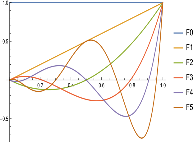
Figure 11: Fubini and Worpitzky polynomials.

Figure 12: $\operatorname{F}_{n}(x)=\sum_{k=0}^{n}(-1)^{n-k}k!\genfrac{\{}{\}}{0.0pt}{}{n}{k}x^{k}.$

Figure 13: $\int_{0}^{1}\operatorname{F}_{n}(x)\,dx=\operatorname{B_{n}}=\int_{0}^{1}\operatorname{F}_{n}(1-x)\,dx.$

20 – The generalized Worpitzky transform

The generalized Worpitzky transform $\operatorname{W}:\mathbb{Z}^{\mathbb{N}}\rightarrow\mathbb{Z}[x]^{\mathbb{N}},\ a\in\mathbb{Z}^{\mathbb{N}},$ maps an integer sequence $a_{0},a_{1},a_{2},\ldots$ to a sequence of polynomials. The $m$-th term of $\operatorname{W}(a)$ is the polynomial $\operatorname{W}_{m}(a)$, given by

$${\operatorname{W}\!\!_{m}(a)\,=\,\sum_{n=0}^{m}(-1)^{n}\binom{m}{n}x^{m-n}\sum_{k=0}^{n}\operatorname{W}(n,k)a_{k}.}$$ (61)

In (61) the inner sum is the Worpitzky transform (60) of $a$. The first few polynomials, $\operatorname{W}_{0},\ldots,\operatorname{W}_{4},$ are:

​ 0pt $$\mathtt{a_{{0}}};\\ \mathtt{a_{{0}}x-(a_{{0}}-a_{{1}}});\\ \mathtt{a_{{0}}{x}^{2}-2\!\left(a_{{0}}-a_{{1}}\right)x+\left(a_{{0}}-3a_{{1}}+2a_{{2}}\right)};\\ \mathtt{a_{{0}}{x}^{3}-3\!\left(a_{{0}}-a_{{1}}\right){x}^{2}+3\!\left(a_{{0}}-3a_{{1}}+2a_{{2}}\right)x-\left(a_{{0}}-7a_{{1}}+12a_{{2}}-6a_{{3}}\right)};\\ \mathtt{a_{{0}}{x}^{4}-4\!\left(a_{{0}}-a_{{1}}\right){x}^{3}+6\!\left(a_{{0}}-3a_{{1}}+2a_{{2}}\right){x}^{2}-4\!\left(a_{{0}}-7a_{{1}}+12a_{{2}}-6a_{{3}}\right)\!x}\\ \mathtt{+\left(a_{{0}}-15a_{{1}}+50a_{{2}}-60a_{{3}}+24a_{{4}}\right).}$$

The definition (61) can be rewritten as

$$\operatorname{W}\!\!_{m}(a)\,=\,\sum_{n=0}^{m}a_{n}\sum_{k=0}^{n}(-1)^{k}\binom{n}{k}(x-k-1)^{m}.$$ (62)

As the reader probably anticipated, we get the Bernoulli polynomials if we set $a_{n}=1/(n+1)$. Evaluating at $x=1$ we arrive at a well-known representation of the Bernoulli numbers:

$$\operatorname{B}_{m}\,=\,\sum_{n=0}^{m}\frac{1}{n+1}\sum_{k=0}^{n}(-1)^{m-k}\binom{n}{k}k^{m},\quad m\geq 0.$$ (63)

It might be noted that if we choose $a_{n}=n+1$ in (62) then the binomial polynomials are obtained. The reader may also enjoy setting $a_{n}={H_{n+1}}$, where ${H}_{n}$ denotes the harmonic numbers.

21 – The Hasse representation

In 1930 Hasse [21] took the next step in the development of formula (63) and proved:

$${\operatorname{B}(s,v)\,=\,\sum_{n=0}^{\infty}\frac{1}{\,n+1\,}\sum_{k=0}^{n}(-1)^{k}\binom{n}{k}(k+v)^{s}}$$ (64)

is an infinite series that converges for all complex $s$ and represents the entire function $-s\zeta(1-s,v)$, the Bernoulli function.

For instance the Hasse series of the central Bernoulli function is

$${\operatorname{B}^{c}(s)\,=\,\sum_{n=0}^{\infty}\frac{1}{\,n+1\,}\sum_{k=0}^{n}(-1)^{k}\binom{n}{k}\left(k+\frac{1}{2}\right)^{s}}.$$ (65)

This representation in turn provides an explicit formula for the central Bernoulli numbers (39),

$${\operatorname{B}^{c}_{n}\,=\,\sum_{j=0}^{n}\frac{1}{\,j+1\,}\sum_{k=0}^{j}(-1)^{k}\binom{j}{k}(2k+1)^{n}}.$$ (66)

An important corollary to Hasse’s formula is: The generalized Bernoulli constants $\beta_{s}(v)$ (23) are given by the infinite series

$$\beta_{s}(v)\,=\,\sum_{n=0}^{\infty}\frac{1}{\,n+1\,}\sum_{k=0}^{n}(-1)^{k}\binom{n}{k}\ln(k+v)^{s}.$$ (67)

For proofs see Blagouchine [8, Cor. 1, formula 123] and the references given there.

22 – The functional equation

The functional equation of the Bernoulli function generalizes a formula of Euler which Graham et al. [18, eq. 6.89] call almost miraculous. But before we discuss it we introduce yet another function and quote a remark from Tao [51].

“It may be that $2\pi i$ is an even more fundamental constant than $2\pi$ or $\pi$. It is, after all, the generator of $\log(1)$. The fact that so many formulas involving $\pi^{n}$ depend on the parity of $n$ is another clue in this regard.”

Taking up this remark we will use the notation $\tau=2\pi i$ and the function

$${\tau(s)}=\tau^{-s}+(-\tau)^{-s}.$$ (68)

We use the principal branch of the logarithm when taking powers of $\tau$. If $s$ is real we can also write $\tau(s)=2^{1-s}\pi^{-s}\cos(\pi s/2)$.

This notation allows us to express the functional equation of the Riemann zeta function [45] as the product of three functions,

$$\zeta\!\left(1-s\right)=\zeta\!\left(s\right)\tau(s)\,\Gamma(s)\qquad(s\in\mathbb{C}\setminus\{0,1\}).$$ (69)

Using (69) and $\operatorname{B}(s)=-s\zeta(1-s)$ we get the representation

$${\operatorname{B}(s)=-\zeta(s)\,\tau(s)\,s!.}$$ (70)

From $\operatorname{B}(1-s)=(s-1)\zeta(s)$ we obtain a self-referential representation of the Bernoulli function, the functional equation

$${\operatorname{B}(s)=\frac{\operatorname{B}(1-s)}{1-s}\tau(s)\,s!\,.}$$ (71)

This functional equation also has a symmetric variant, which means that the left side of (72) is unchanged by the substitution $s\leftarrow 1-s$.

$$\operatorname{B}(1-s)\,\left(\frac{s}{2}\right)!\ \pi^{-s/2}\,=\,\operatorname{B}(s)\left(\frac{1-s}{2}\right)!\ \pi^{-(1-s)/2}.$$ (72)

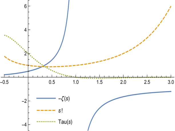
Figure 14: The Riemann decomposition of the Bernoulli function (70).

23 – Representation by the Riemann $\xi$ function

The right (or the left) side of (72) turns out to be the Riemann $\xi$ function,

$$\xi(s)\,=\,\left(\frac{s}{2}\right)!\ \pi^{-s/2}\,(s-1)\zeta(s).$$ (73)

For a discussion of this function see for instance Edwards [14]. Thus we get a second representation of the Bernoulli function in terms of a Riemann function:

$${\operatorname{B}(s)\,=\,\frac{\pi^{(1-s)/2}}{\left((1-s)/2\right)!}\ \xi(s)\,.}$$ (74)

By the functional equation of $\xi$, $\xi(s)=\xi(1-s)$, we also get

$${\operatorname{B}(1-s)\,=\,\frac{\pi^{s/2}}{\left(s/2\right)!}\ \xi(s)\,.}$$ (75)

This is a good opportunity to check the value of $\operatorname{B}(-1)$.

$${\operatorname{B}(-1)\,=\,\pi\,\xi(-1)=\,\frac{\pi^{2}}{6}=\pi\,\xi(2)\,.}$$ (76)

In this row of identities, the names Bernoulli, Euler (solving the Basel problem in 1734), and Riemann join together.

Figure 15: The Hadamard decomposition of the Bernoulli function.

24 – The Hadamard decomposition

We denote Hadamard’s infinite product over the zeros of $\zeta(s)$ by

$$\operatorname{H}_{\zeta}(s)\,=\,\frac{1}{2}\,\prod_{\mathop{\rm Im}\nolimits{\rho}>0}\left(1-\frac{s}{\rho}\right)\left(1-\frac{s}{1-\rho}\right).$$ (77)

The product runs over the zeros with $\mathop{\rm Im}\nolimits(\rho)>0$. The absolute convergence of the product is guaranteed as the terms are taken in pairs $(\rho,1-\rho)$. Hadamard’s infinite product expansion of $\zeta(s)$ is

$$\zeta(s)\,=\,\frac{\pi^{s/2}}{\left(s/2\right)!}\,\frac{\operatorname{H}_{\zeta}(s)}{s-1}\,,\quad s\notin\{1,-2,-4,\dots\}.$$ (78)

Since the zeros of $\zeta(s)$ and $\operatorname{B}(s)$ are identical in the critical strip by (70), this representation carries directly over to the Bernoulli case. Writing $\sigma=(1-s)/2$ we get (see figure 15)

$${\operatorname{B}(s)\,=\,\frac{\pi^{\sigma}}{\sigma!}\,\operatorname{H}_{\zeta}(s)\,,\quad s\notin\{-2,-4,-6,\dots\}.}$$ (79)

This is the Hadamard decomposition of the Bernoulli function.

The zeros of $\operatorname{B}(s)$ with $\mathop{\rm Im}\nolimits(\rho)=0$ are at $3,5,7,\ldots$ (making the Bernoulli numbers vanish at these indices), due to the factorial term in the denominator. This representation separates the nontrivial zeros on the critical line from the trivial zeros on the real axes.

Here we see one more reason why $\operatorname{B}_{1}=\frac{1}{2}$. The oscillating factor has the value $\frac{\pi^{0}}{0!}=1,$ and the Hadamard factor has the value $\operatorname{H}_{\zeta}(1)=-\zeta(0)\cdot 1$. The Bernoulli value follows from $\zeta(0)=-\frac{1}{2}$.

If we compare the identities $(\ref{q554})$ and $(\ref{q56})$, we get as a corollary ${\xi=\operatorname{H}_{\zeta}}.$ This is precisely the proposition that Hadamard proves in his 1893 paper [19]. Thus applying (28) to (78) leads to Jensen’s formula for the Riemann $\xi$ function,

$$\xi(s)\,=\,\frac{2(s/2)!}{\pi^{s/2-1}}\int_{-\infty}^{\infty}\frac{(\tfrac{1}{2}+ix)^{1-s}}{({\mathrm{e}}^{\pi x}+{\mathrm{e}}^{-\pi x})^{2}}\,dx.$$ (80)

25 – The generalized Euler function

The generalized Euler function is defined in terms of the generalized Genocchi function (44) as

$$\operatorname{E}(s,v)\,=\,-\frac{\operatorname{G}(s+1,v)}{s+1}.$$ (81)

Of particular interest are the cases $v=1$ and $v=1/2$ which we will consider now.

26 – The Euler tangent function

The Euler tangent function is defined as

$$\operatorname{E}_{\tau}(s)\,=\,2^{s}\operatorname{E}(s,1),$$ (82)

where the limiting value $\log(2)$ closes the definition gap at $s=-1.$

An alternative representation is $\operatorname{E}_{\tau}(s)=-2\operatorname{\mathop{\rm Re}\nolimits}({\operatorname{Li}_{-s}(i)})$, where $\operatorname{Li}_{s}(v)$ denotes the polylogarithm.

Of special interest is formula (82) for integer values $n$,

$$\operatorname{E}_{\tau}(n)\,=\,2^{n}\operatorname{E}(n,1)\quad(n\geq 0).$$ (83)

These numbers are listed in OEIS A155585; the first few values are

$$\operatorname{E}_{\tau}(n)\,=\,1,\,1,\,0,\,-2,\,0,\,16,\,0,\,-272,\,0,\,7936,\,0,\,-353792,\,\ldots$$

Tracing back the definitions and using (36), the Bernoulli function can express the Euler tangent function as

$$\operatorname{E}_{\tau}(s)\,=\,\left(4^{s+1}-2^{s+1}\right)\frac{\operatorname{B}(s+1)}{s+1}.$$ (84)

The Euler tangent numbers are of particular importance because they relate the numbers $\operatorname{E}_{\tau}(n)$ to another type of Euler numbers, the Eulerian numbers.

Let $\genfrac{<}{>}{0.0pt}{}{n}{k}$ denote the Eulerian numbers OEIS A173018, then

$$\operatorname{E}_{\tau}(n)\,=\,\sum_{k=0}^{n}(-1)^{k}\genfrac{<}{>}{0.0pt}{}{n}{k}.$$ (85)

The right side of (85) is the value of the Eulerian polynomial [38] $\mathrm{A}_{n}(x)=\sum_{k=0}^{n}\genfrac{<}{>}{0.0pt}{}{n}{k}x^{k}$ at $x=-1$. With this we get the identity

$$2^{n}\operatorname{E}_{n}(1)\,=\,\operatorname{E}_{\tau}(n)\,=\,\mathrm{A}_{n}(-1).$$ (86)

A further representation results if the factor $2^{n}$ is taken into account in the Stirling-Fubini representation of the Bernoulli numbers. Indeed, $\operatorname{E}_{\tau}(n)=\operatorname{P}_{n}(1)$ where

$$\operatorname{P}_{n}(x)=\sum_{k=0}^{n}(-2)^{n-k}\genfrac{\{}{\}}{0.0pt}{}{n}{k}k!\,x^{k}.$$ (87)

27 – The Euler secant function

Figure 16: Euler tangent versus Euler secant function.

The Euler secant function is defined

$$\operatorname{E}_{\sigma}(s)\,=\,2^{s}\operatorname{E}\left(s,1/2\right),$$ (88)

with the limiting value $\operatorname{E}_{\sigma}(-1)\,=\,\pi/2.$

We also write $\operatorname{E}(s)=\operatorname{E}_{\sigma}(s)$ and call this function the Euler function, because it interpolates the numbers

$$\operatorname{E}_{n}\ =\ \operatorname{E}_{\sigma}(n)\ =\ 2^{n}\operatorname{E}\left(n,1/2\right)\quad(n\geq 0),$$ (89)

which traditionally are called the Euler numbers.

The OEIS identifier is A122045 and the sequence starts

$$\operatorname{E}_{n}\,=1,\,0,\,-1,\,0,\,5,\,0,\,-61,\,0,\,1385,\,0,\,-50521,\,0,\,2702765,\,\ldots$$

The generalized Bernoulli function can represent the Euler secant function as

$$\operatorname{E}_{\sigma}(s)\,=\,\frac{2}{s+1}\,4^{s}\left(\operatorname{B}\left(s+1,\frac{3}{4}\right)-\operatorname{B}\left(s+1,\frac{1}{4}\right)\right).$$ (90)

A more compact form is $\operatorname{E}_{\sigma}(s)=2\operatorname{\mathop{\rm Im}\nolimits}(\operatorname{Li}_{-s}(i))$.

The Jensen formula for the even-indexed classical Euler numbers follows from (90) and the Jensen formula (30) for the generalized Bernoulli function.

$$\operatorname{E}_{2n}\,=\,\frac{2\pi}{2n+1}\int_{0}^{\infty}\frac{(4zi+1)^{2n+1}-(4zi-1)^{2n+1}}{({\mathrm{e}}^{-\pi z}+{\mathrm{e}}^{\pi z})^{2}}\,dz.$$ (91)

28 – The family of Bernoulli and Euler numbers

The family tree of the Euler numbers is subdivided into three branches: the Euler secant numbers, the Euler tangent numbers, and the Euler zeta numbers. The Euler zeta numbers are rational numbers, whereas the Euler secant and Euler tangent numbers are integers.

The traditional way of naming reserves the name ‘Euler numbers’ for the Euler secant numbers, while the way preferred by combinatorialists (see for instance Stanley [48]) is to call Euler numbers what we call the André numbers.

We introduce the name ‘André numbers’ in honor of Désiré André, who studied their combinatorial interpretation as $2$-alternating permutations in 1879 and 1881 [2, 3]. We believe that this is a fair sharing of the mathematical name space and eliminates the ambiguity that otherwise exists.

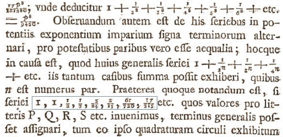
Figure 17: L. Euler, De summis serierum reciprocarum, 1735.

$n$	1	2	3	4	5	6	7	8
$\operatorname{E}_{\sigma}$	$0$	$-1$	$\ 0$	$5$	$0$	$-61$	$\ \ 0$	$1385$
$\operatorname{E}_{\tau}$	$1$	$0$	$-2$	$0$	$16$	$0$	$-272$	$0$
$\mathcal{A}$	$1$	$1$	$\ \ 2$	$5$	$16$	$\ \ 61$	$\ \ 272$	$1385$

Table 5: Euler and André numbers

Let us try to replicate the above extension procedure for the Bernoulli numbers. The next table shows the outcome of our choice.

$n$	1	2	3	4	5	6	7	8
$\operatorname{B}_{\tau}$	$0$	$\frac{1}{6}$	$0$	$-\frac{1}{30}$	$0$	$\frac{1}{42}$	$0$	$-\frac{1}{30}$
$\operatorname{B}_{\sigma}$	$\frac{1}{2}$	$\ 0$	$-\frac{3}{56}$	$\ \ 0$	$\frac{25}{992}$	$0$	$-\frac{427}{16256}$	$\ \ 0$
$\mathcal{S}$	$\frac{1}{2}$	$\frac{1}{6}$	$\ \ \frac{3}{56}$	$\ \ \frac{1}{30}$	$\frac{25}{992}$	$\frac{1}{42}$	$\ \ \frac{427}{16256}$	$\ \ \frac{1}{30}$

Table 6: Bernoulli and Seki numbers

We introduce the name ‘Seki numbers’ in honor of Takakazu Seki, who discovered Bernoulli numbers before Jacob Bernoulli (see [30]) to denote the extended version of the Bernoulli numbers in their unsigned form, which is the third row in the table above.

The relationship between the seven sequences is shown in figure 18. It reveals that the Bernoulli numbers and the Euler numbers have a common backbone: the Euler zeta numbers. Euler introduced these rational numbers in 1735 in De summis serierum reciprocarum [16]. We will denote the numbers with $\mathcal{Z}_{n}$. They begin for $n\geq 0$

$$1,\ 1,\ \frac{1}{2},\ \frac{1}{3},\ \frac{5}{24},\ \frac{2}{15},\ \frac{61}{720},\ \frac{17}{315},\ \frac{277}{8064},\ \frac{62}{2835},\ldots.$$ (92)

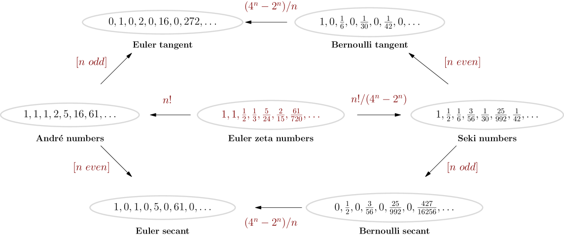
Figure 18: .
The Euler–Bernoulli family of numbers (unsigned version)

29 – The Bernoulli secant numbers

The Bernoulli secant function $\operatorname{B}_{\sigma}$ is defined by the equation

$$\operatorname{B}_{\sigma}(s)\,=\,\frac{2^{s-1}}{2^{s}-1}\left(\operatorname{B}\left(s,\frac{3}{4}\right)-\operatorname{B}\left(s,\frac{1}{4}\right)\right).$$ (93)

Bernoulli secant numbers are for integer $n\geq 1$ the values of the Bernoulli secant function and by convention $\operatorname{B}^{\sigma}_{0}=0$.

$$\operatorname{B}^{\sigma}_{n}\,=\,0,\ \frac{1}{2},\ 0,\ -\frac{3}{56},\ 0,\ \frac{25}{992},\ 0,\ -\frac{427}{16256},\ 0,\ \ldots$$ (94)

Thus, if one calls the classical Bernoulli numbers the Bernoulli tangent numbers $\operatorname{B}^{\tau}_{n}$, one gets a way of speaking that corresponds to the classical terminology associated with the Euler numbers. See figure 18, and OEIS A160143, A193476.

The Bernoulli secant numbers can be represented by the Euler secant numbers since

$$\operatorname{B}_{\sigma}(n)\,=\,(-1)^{n-1}\frac{n}{4^{n}-2^{n}}\operatorname{E}_{\sigma}(n-1)\quad(n\geq 1).$$ (95)

From (90) and (93) we see that this is a special case of

$$\operatorname{B}_{\sigma}(s)\,=\,\frac{2s}{4^{s}-2^{s}}\operatorname{\mathop{\rm Im}\nolimits}(\operatorname{Li}_{1-s}(i)).$$ (96)

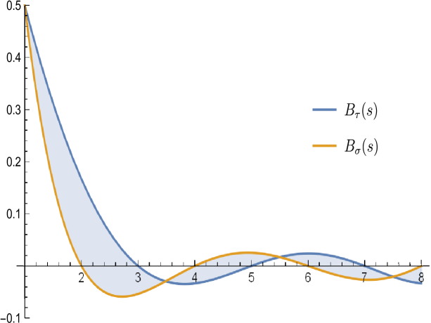
Figure 19: Bernoulli tangent versus Bernoulli secant function.

30 – The extended Bernoulli function

The extended zeta function is defined for $s\neq 1$ as

$${\widetilde{\zeta}(s)\,=\,\zeta\left({s}\right)-\frac{\zeta\left({s},{\frac{3}{4}}\right)-\zeta\left({s},{\frac{1}{4}}\right)}{{2}^{{s}}-2}.}$$ (97)

The extended Bernoulli function is defined for $s\neq 0$ as

$${\mathcal{B}(s)\,=\,-s\,\widetilde{\zeta}(1-s).}$$ (98)

Setting $\mathcal{B}(0)=1+{\pi}/{\log(4)}$ closes the definition gap.

An equivalent definition using the generalized Bernoulli function is

$$\mathcal{B}(s)\,=\,\operatorname{B}(s)+\frac{2^{s-1}}{2^{s}-1}\left(\operatorname{B}\left(s,\frac{3}{4}\right)-\operatorname{B}\left(s,\frac{1}{4}\right)\right).$$ (99)

With the terms introduced above, this says that the extended Bernoulli function is the the sum of the tangent Bernoulli and the secant Bernoulli function.

$$\mathcal{B}(s)\,=\operatorname{B}_{\tau}(s)+\operatorname{B}_{\sigma}(s).$$ (100)

The extended Bernoulli numbers are the values of the extended Bernoulli function at the positive integers.

$$1,\ \frac{1}{6},\ -\frac{3}{56},\ -\frac{1}{30},\ \frac{25}{992},\ \frac{1}{42},\ -\frac{427}{16256},\ -\frac{1}{30},\ \ldots$$ (101)

31 – The extended Euler function

The extended Euler function is a generalization of the identity (84),

$$\mathcal{E}(s)\, =\,\left(4^{s+1}-2^{s+1}\right)\frac{\mathcal{B}(s+1)}{(s+1)},$$ (102)

$$=\,(2^{s+1}-4^{s+1})\,\widetilde{\zeta}(-s).$$ (103)

The limiting value $\pi/2+\log(2)$ closes the definition gap at $s=-1$.

The extended Euler function is the sum of the Euler secant and the Euler tangent function.

$$\mathcal{E}(s)\,=\,\operatorname{E}_{\sigma}(s)+\operatorname{E}_{\tau}(s)\,=\,2^{s}(\operatorname{E}\left(s,1/2\right)+\operatorname{E}\left(s,1\right)).$$ (104)

For integer $n\geq 0$ we write $\mathcal{E}_{n}=\mathcal{E}(n)$. The sequence starts:

$$\mathcal{E}_{n}=2,\,1,\,-1,\,-2,\,5,\,16,\,-61,\,-272,\,1385,\,\dots.$$ (105)

These are the extended Euler numbers $\mathcal{E}_{n}$, OEIS A163982 negated.

Since $\operatorname{B}(s,1/2)=\operatorname{B}(s)(2^{1-s}-1)$, the difference of the right-hand sides of (90) and (84) reduces to

$$\mathcal{E}(s)\,=\,\frac{(4^{s+1}-2^{s+2}+2)\operatorname{B}(s+1)-4^{s+1}\operatorname{B}(s+1,1/4)}{s+1}.$$ (106)

The Jensen representation follows from (106).

$$\mathcal{E}(s)\,=\,\frac{2\pi}{s+1}\int_{\infty}^{\infty}\frac{(4zi+1)^{s+1}+(1-2^{-2s-1})(2+4zi)^{s+1}}{({\mathrm{e}}^{-\pi z}+{\mathrm{e}}^{\pi z})^{2}}\,dz.$$ (107)

32 – The André function

Many of the traditional integer sequences considered here are signed, like the Bernoulli numbers and the Euler numbers. However, under the influence of combinatorics, more and more the unsigned versions of these numbers have come into focus. The paradigmatic example are the absolute Euler numbers, which we call André numbers.

The unsigned versions of the Euler secant and Euler tangent functions are defined as

$$\operatorname{|E|}_{\sigma}(s)\,=\,\cos(\pi s/2)\operatorname{E}_{\sigma}(s);$$ (108)

$$\operatorname{|E|}_{\tau}(s)\,=\,\sin(\pi s/2)\operatorname{E}_{\tau}(s).$$ (109)

The André function is defined as the sum of these two unsigned Euler functions,

$${\mathcal{A}(s)\,=\,\operatorname{|E|}_{\sigma}(s)+\operatorname{|E|}_{\tau}(s).}$$ (110)

Considering the long chain of definitions on which (110) is based, it is astonishing how easily it can be represented by a single function.

$${\mathcal{A}(s)\,=\,(-i)^{s+1}\operatorname{Li}_{-s}(i)+i^{s+1}\operatorname{Li}_{-s}(-i).}$$ (111)

Here $i$ is the imaginary unit, $\operatorname{Li}_{s}(v)$ is the polylogarithm, and the principal branch of the logarithm is used for the powers.

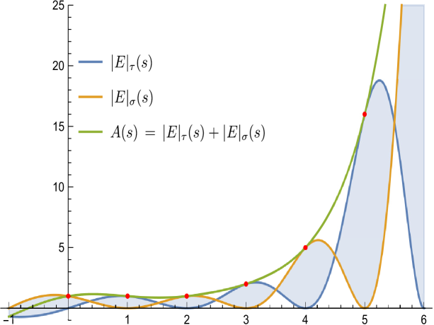
Figure 20: The André function $\mathcal{A}(s).$

The André numbers $\mathcal{A}_{n}=\mathcal{A}(n)$ are listed for integer $n\geq 0$ in OEIS A000111. The sequence starts:

$$\mathcal{A}_{n}=1,\,1,\,1,\,2,\,5,\,16,\,61,\,272,\,1385,\,7936,\,\dots.$$ (112)

For integer $n\geq 1$ equation (111) simplifies to

$$\mathcal{A}_{n}=2\,(-i)^{n+1}\operatorname{Li}_{-n}(i).$$ (113)

The Euler zeta numbers are, by definition,

$${\mathcal{Z}_{n}\,=\frac{\mathcal{A}_{n}}{n!}\quad(n\geq 0).}$$ (114)

The signed André function $\mathcal{A}^{\ast}(s)$ interpolates the signed André numbers $\mathcal{A}^{\ast}_{n}=(-1)^{n}\mathcal{A}_{n},$ and is defined as

$$\mathcal{A}^{\ast}(s)\,=\,ie^{-\frac{1}{2}i\pi s}\left(\text{Li}_{-s}(-i)-e^{i\pi s}\text{Li}_{-s}(i)\right).$$ (115)

The signed André numbers are OEIS A346838, and differ from (105) in the first term and by the sign pattern.

$$\mathcal{A}^{\ast}_{n}=1,\,-1,\,1,\,-2,\,5,\,-16,\,61,\,-272,\,1385,\,\dots.$$ (116)

33 – The Seki function

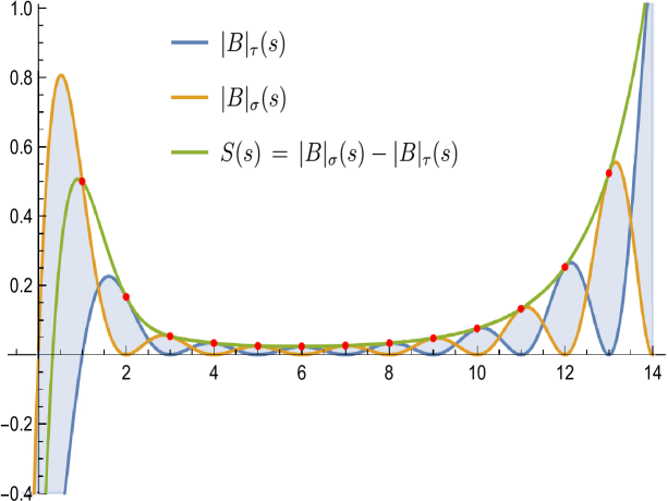
Figure 21: The Seki function $\mathcal{S}(s).$

The unsigned versions of the Bernoulli secant and Bernoulli tangent functions are defined as

$$\operatorname{|B|}_{\sigma}(s)\,=\,\sin(\pi s/2)\operatorname{B}_{\sigma}(s);$$ (117)

$$\operatorname{|B|}_{\tau}(s)\,=\,\cos(\pi s/2)\operatorname{B}_{\tau}(s).$$ (118)

The Seki function is defined as the difference of these two unsigned Bernoulli functions,

$${\mathcal{S}(s)\,=\,\operatorname{|B|}_{\sigma}(s)-\operatorname{|B|}_{\tau}(s).}$$ (119)

One can also base the Seki function on the André function $\mathcal{A}$. For $s=0$ we set the limiting value, $\mathcal{S}(0)=-1$, and otherwise

$${\mathcal{S}(s)\,=\,\frac{s\,\mathcal{A}(s-1)}{4^{s}-2^{s}}\quad(s\neq 0).}$$ (120)

In terms of the polylogarithm this is

$${\mathcal{S}(s)\,=\,\frac{s}{4^{s}-2^{s}}\left((-i)^{s}\operatorname{Li}_{1-s}(i)+i^{s}\operatorname{Li}_{1-s}(-i)\right)\quad(s\neq 0).}$$ (121)

The Seki function ${\mathcal{S}}$ interpolates the absolute values of the extended Bernoulli numbers for $n\geq 1$. The Seki numbers are $\mathcal{S}_{n}=\mathcal{S}(n)$ if $n\geq 1$, and $\mathcal{S}_{0}=1$ by convention.

The signed Seki function $\mathcal{S}^{\ast}(s)$ interpolates the signed Seki numbers $\mathcal{S}^{\ast}_{n}=(-1)^{n}\mathcal{S}_{n},$ and is defined as $\mathcal{S}^{\ast}(0)=1$, and otherwise

$$\mathcal{S}^{\ast}(s)\,=\,\frac{s}{2^{s}-4^{s}}\,e^{i\pi s/2}\left(e^{i\pi s}\text{Li}_{1-s}(-i)+\text{Li}_{1-s}(i)\right).$$ (122)

The signed Seki numbers differ from (105) in the first two terms and by the sign pattern. Apart from the signs, this is the sequence OEIS A193472/A193473.

34 – The Swiss-knife polynomials

The Euler equivalent to the central Bernoulli polynomials is the sequence of Swiss-knife polynomials (see figure 22), defined as the Appell sequence associated with the Euler numbers $\operatorname{E}_{n}$.

$$\operatorname{K}_{n}(x)\,=\,\sum_{k=0}^{n}\binom{n}{k}\operatorname{E}_{k}x^{n-k}.$$ (123)

$1$
$x$
${x}^{2}\,-\,1$
${x}^{3}\,-\,3\,x$
${x}^{4}\,-\,6\,x^{2}\,+\,5$
$x^{5}\,-\,10\,x^{3}\,+\,25\,x$
$x^{6}\,-\,15\,x^{4}\,+\,75\,x^{2}\,-\,61$
$x^{7}\,-\,21\,x^{5}\,+\,175\,x^{3}\,-\,427\,x$
$x^{8}\,-\,28\,x^{6}\,+\,350\,x^{4}\,-\,1708\,x^{2}\,+\,1385$
$x^{9}\,-\,36\,x^{7}\,+\,630\,x^{5}\,-\,5124\,x^{3}\,+\,12465\,x$

Table 7: The Swiss-knife polynomials ${{{\kappa}}}_{n}(x)$ for $n\geq 0.$

They were introduced in OEIS A153641 and A081658. The author discussed them in [36] and dubbed them Swiss-knife polynomials $\operatorname{K}_{n}(x)$ because they allow calculating the Euler–Bernoulli family of numbers efficiently. The coefficients of the polynomials are integers, in contrast to the coefficients of the Euler and Bernoulli polynomials. The parity of the monic $\operatorname{K}_{n}(x)$ equals the parity of $n$.

The Worpitzky representation of the Swiss-knife polynomials is the generalized Worpitzky transform (62) of the sequence $\nu(n)$, where $\nu(n)=\cos((n-1)\pi/4)/2^{(n-1)/2}$.

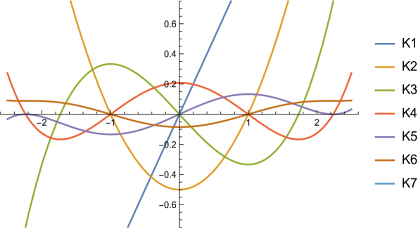
Figure 22: The Swiss knife polynomials ${{{\kappa}}}_{n}(x)/n!$

Equivalently, let $\alpha$ be the repeating sequence with period $p$, where $p=(1,1,1,0,-1,-1,-1,0)$, then

$${\operatorname{K}_{n}(x)=\sum_{k=0}^{n}\frac{\alpha(k)}{2^{\lfloor k/2\rfloor}}\sum_{v=0}^{k}(-1)^{v}\binom{k}{v}(x+v+1)^{n}.}$$ (124)

Chen [11, theorem 3] proves (124) for the Euler numbers $\operatorname{K}_{n}(0)$ and $\operatorname{K}_{n}(1)$ using the Akiyama–Tanigawa algorithm.

The Swiss-knife polynomials can be computed efficiently with the following recurrence:

 

Set $\operatorname{K}_{0}(x)=1$ for all $x$.

Now assume $\operatorname{K}_{n-1}(x)$ already computed and take the coefficients

$$c_{k}^{(n-1)}=[x^{n-2k}]\operatorname{K}_{n-1}(x)\text{ for }k\in\{0,1,\ldots,\lfloor(n-1)/2\rfloor\}.$$

Next compute

$$c_{k}^{(n)}=c_{k}^{(n-1)}n/(n-2k)\ \ \text{for }k\in\{0,1,\ldots,\lfloor(n-1)/2\rfloor\}.$$ (125)

If $n$ is even, set additionally $c_{n/2}^{(n)}=-\sum_{k=0}^{\lfloor(n-1)/2\rfloor}c_{k}^{(n)}$. Then

$$\operatorname{K}_{n}(x)=\sum_{k=0}^{\lfloor n/2\rfloor}c_{k}^{(n)}x^{n-2k}.$$ (126)

 

The algorithm is based on the fact that the Swiss-knife polynomials form an Appell sequence.

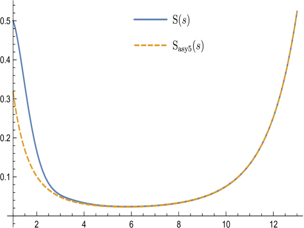
Figure 23: Approximation to the Seki function.

Figure 24: $\mathcal{S}(s)\,\simeq\,2^{\frac{3}{2}-s}\pi^{\frac{1}{2}-s}s^{s+\frac{1}{2}}e^{\frac{(2/7)-s^{2}+30s^{4}-360s^{6}}{360s^{5}}}$

35 – Asymptotics for the Bernoulli function

An asymptotic expansion of the Bernoulli function follows directly from $\operatorname{B}(s)=-\zeta(s)\,\tau(s)\,s!$ by using Stirling’s formula and the generalized harmonic numbers.

For the remainder term we will use the notation

$$\operatorname{R_{K}}(s)\,=\,\exp\left(\frac{1}{2}+\sum_{n=1}^{\operatorname{K}}\frac{\operatorname{B}(n+1)}{n+1}\frac{s^{-n}}{n}\right).$$ (127)

For an even positive integer $n$, the Bernoulli function has an efficient asymptotic approximation [34], which reads with $\operatorname{R_{5}}(s)$

$${|\operatorname{B}(n)|\,\sim\,4\,\pi\,\left(\frac{n}{2\pi\mathrm{e}}\right)^{n+1/2}\exp\left(\frac{1}{2}+\frac{n^{-1}}{12}-\frac{n^{-3}}{360}+\frac{n^{-5}}{1260}\right).}$$ (128)

The coefficients originate from the Stirling expansion of $\log(\Gamma(s))$ (see A046969).

The number of exact decimal digits guaranteed by (128) is $3\log(3\,n)$ if $n\geq 50$. The Boost $\operatorname{C}^{++}$ library [10] uses this approximation for huge arguments $n$.

Different asymptotic developments can be based on other expansions of the Gamma function, for instance, on Binet’s formula [15, p. 48, A122252] generalized by Nemes [42, 4.2]. More general asymptotic expansions and error bounds follow from those of the Hurwitz zeta function established in Nemes [43].

But much more is true: The assumption made for (128) that $n$ is an even positive integer can be dropped if one adds the factor $-\cos\left(\frac{s\pi}{2}\right)$ to the right side. This gives the asymptotic expansion of the Bernoulli function for real $s>0$, with $\operatorname{K}$ suitably chosen,

$$\operatorname{B}(s)\,\sim\,4\,\pi\,\left({\frac{s}{{{2\pi\mathrm{e}}}}}\right)^{s+1/2}\left(-\cos\left(\frac{s\pi}{2}\right)\right)\operatorname{R}_{\operatorname{K}}(s).$$ (129)

Moreover, the Seki $\mathcal{S}(s)$ has the corresponding expansion without the factor $-\cos\left(\frac{s\pi}{2}\right)$.

The close connection between the Bernoulli and the Euler numbers is also reflected in the fact that the asymptotic development of the Euler function differs formally only slightly from (129).

$$\operatorname{E}(s)\,\simeq\,-4\,\left({\frac{2s}{{{\pi\mathrm{e}}}}}\right)^{s+1/2}\left(-\cos\left(\frac{s\pi}{2}\right)\right)\operatorname{R}_{\operatorname{K}}(s).$$ (130)

From (129) and (130) asymptotic expansions for other functions can be easily derived. As an example we show an asymptotic expansion of the logarithm of the André function of order $O(s^{-7})$.

$$\log\mathcal{A}(s)\ \simeq\ \log(4)+\left(\frac{1}{2}+s\right)\log\left(\frac{2s}{\pi}\right)+\frac{(2/7)-s^{2}+30s^{4}-360s^{6}}{360s^{5}}$$ (131)

36 – Definition dependencies

In the present essay we have entirely dispensed with generating functions and have only taken the analytical point of view. This resulted in a net of hierarchically structured definitions shown in the graph 25 below. The numbers attached to the arrows indicate the corresponding formula.

This shows that all functions of the Euler-Bernoulli family can be represented using the central formula (30). This approach is not just theoretically interesting; it might also offer computational advantages.

To this end, we note that integrals of the Jensen type can be evaluated numerically efficiently to high accuracy. Based on Johansson and Blagouchine [28] relevant routines were implemented by Johansson in an arbitrary-precision software library [27] with rigorous bounds and used to compute the Stieltjes constants.

Further expansion of this computational infrastructure to the Hurwitz-Bernoulli function providing an alternative to the Hurwitz-Riemann function would be highly desirable.

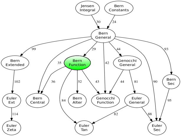
Figure 25: Dependency graph of definitions.

37 – Epilogue: Generating functions

The value of $\operatorname{B}(1)$ deserves special attention. Since it is well known that $\sum_{j=0}^{\infty}{\gamma_{j}}/{j!}=1/2$, it follows from (8) that $\operatorname{B}(1)=1/2$. Unfortunately, the popular generating function $z/(\mathrm{e}^{z}-1)$ misses this value and disrupts at this point the connection between the Bernoulli numbers and the $\zeta$ function.

For those who do not care about the connection with the zeta function, we add: Even the most elementary relations between the Bernoulli numbers and the Bernoulli polynomials break with this choice. For instance, consider the basic identity (41). It applies to all Bernoulli numbers if $\operatorname{B}_{n}=\operatorname{B}_{n}(1)$ but not if $\operatorname{B}_{n}=\operatorname{B}_{n}(0)$ is set.

Many other relations get restricted in their range of validity if the wrong choice is made, for example, the relation between the Bernoulli numbers and the Eulerian numbers. Such examples are described in the discussion [33].

Instead, use the power series $f(z)$ with the constant term $1$ such that the coefficient of $x^{n}$ in $(f(x))^{n+1}$ equals $1$ for all $n$. There is only one power series satisfying this condition, as Hirzebruch [23] observes.

This series is the Todd function (called after John Arthur Todd)

$${\operatorname{T}(z)\,=\,\frac{z}{1-\mathrm{e}^{-z}}\,=\,1+\frac{1}{2}\frac{z}{1!}+\frac{1}{6}\frac{z^{2}}{2!}-\frac{1}{30}\frac{z^{4}}{4!}+\ldots}.$$ (132)

It generates the Bernoulli numbers matching the values of the Bernoulli function at the nonnegative integers.

A modern exposition based on the Todd series is the monograph of Arakawa, Ibukiyama, and Kaneko [5]. The authors adopt this definition “because it is the original definition of Seki and Bernoulli for one thing, and it is better suited to the special values of the Riemann zeta function for another.”

Similarly, Neukirch in Algebraic Number Theory [44] calls the definition $f(z)=z/(1-\mathrm{e}^{-z})$ “more natural and better suited for the further development of the theory.” One might hope that all mathematicians will support this simple step towards greater consistency someday.

38 – Acknowledgments

The author thanks Jörg Arndt, Petros Hadjicostas, Václav Kotěšovec, Richard J. Mathar, Gergő Nemes, and Michael Somos for their reading and providing valuable feedback on an earlier version of this manuscript. Thanks to Michel Marcus and Jon E. Schoenfield for help with proofreading.

Without using Neil Sloane’s OEIS this essay could have been written, but it would only have been half as much fun.

Figure 26: ‘Don Quixote’, sketch by Pablo Picasso.

Some applications of the Swiss-knife polynomials, where

$\alpha_{n}={n}/(4^{n}-2^{n}),$ and by convention $\operatorname{K}_{-1}(x)=1.$

$\frac{\href http://www.oeis.org/A099612}{\href http://www.oeis.org/A099617}$	Euler zeta	$\mathcal{E}(n)\,=\,\lvert\operatorname{K}_{n}(n\bmod 2)\rvert\,/\,n!$
A000111	Euler numbers	$\operatorname{E}(n)\,=\,\operatorname{K}_{n}(n\bmod 2)$
A028296	Euler secant	$\operatorname{E}_{\sigma}(2n)\,=\,\operatorname{K}_{2n}(0)$
A000182	Euler tangent	$\operatorname{E}_{\tau}(2n+1)\,=\,\operatorname{K}_{2n+1}(1)$
$\frac{\href http://www.oeis.org/A164555}{\href http://www.oeis.org/A027642}$	Bernoulli numbers	$\operatorname{B}(n)\,=\,\operatorname{K}_{n-1}(1)\,\alpha_{n}$
$\frac{\href http://www.oeis.org/A000367}{\href http://www.oeis.org/A002445}$	Bernoulli tangent	$\operatorname{B}_{\tau}(2n)\,=\,\operatorname{K}_{2n-1}(1)\,\alpha_{2n}$
$\frac{\href http://www.oeis.org/A160143}{\href http://www.oeis.org/A193476}$	Bernoulli secant	$\operatorname{B}_{\sigma}(2n+1)\,=\,\operatorname{K}_{2n}(0)\,\alpha_{2n+1}$
$\frac{\href http://www.oeis.org/A193472}{\href http://www.oeis.org/A193473}$	Bernoulli extend.	$\mathcal{B}(n)\,=\,\operatorname{K}_{n-1}((n-1)\,\bmod\,2)\,\alpha_{n}$
A226158	Genocchi	$\operatorname{G}(n)\,=\,-\operatorname{K}_{n-1}(-1)\,n\,/\,2^{n-1}$
A188458	Springer	$\operatorname{S}(n)\,=\,\operatorname{K}_{n}(1/2)\,2^{n}$

Concerned with sequences A001896, A001897, A019692, A027642, A028246, A081658, A099612, A099617, A122045, A153641, A155585, A160143, A163626, A163747, A164555, A173018, A193472, A193473, A193476, A226158, A263634, A278075, A301813, A303638, A318259, A333303, A335263, A335750, A335751, A335947, A335948, A335949, A335953, A336454, A336517, A337966, A337967, A342317, A344917, A344918, A346463, A346464, A346832, A346833, A346834, A346835, A346838 and A344913.

 

2020 MSC: Primary 11B68, Secondary 11M35.

Keywords: Bernoulli function, Bernoulli constants, Bernoulli numbers, Bernoulli cumulants, Bernoulli functional equation, Bernoulli central function, extended Bernoulli function, Bernoulli central polynomials, alternating Bernoulli function, Stieltjes constants, Riemann zeta function, Hurwitz zeta function, Worpitzky numbers, Worpitzky transform, Hasse representation, Hadamard product, Genocchi numbers, Genocchi function, Euler secant numbers, Euler tangent numbers, Euler zeta numbers, Euler function, Euler tangent function, Euler secant function, Eulerian numbers, André numbers, André function, Seki numbers, Seki function, Swiss-knife polynomials.

 

Software: Code repository and supplements, including a Maple worksheet and a Mathematica Jupyter notebook, available at GitHub [39].

Author: ORCID 0000-0001-6245-708X

39 – Bernoulli constants

$\qquad\qquad\qquad\beta_{n}\quad\qquad\qquad\qquad\qquad\qquad b_{n}=\frac{\beta_{n}}{n!}$

   [ 0]  +1.00000000000000000000000e+00   +1.00000000000000000000000e+00   [ 1]  -5.77215664901532860606512e-01   -5.77215664901532860606512e-01   [ 2]  +1.45631690967353449721173e-01   +7.28158454836767248605864e-02   [ 3]  +2.90710895786169554535912e-02   +4.84518159643615924226519e-03   [ 4]  -8.21533768121338346464019e-03   -3.42305736717224311026674e-04   [ 5]  -1.16268503273365002873409e-02   -9.68904193944708357278404e-05   [ 6]  -4.75994290380637621052001e-03   -6.61103181084218918127779e-06   [ 7]  +1.67138541801139726910695e-03   +3.31624090875277235933919e-07   [ 8]  +4.21831653646200836859278e-03   +1.04620945844791874221051e-07   [ 9]  +3.16911018422735558641847e-03   +8.73321810027379736116201e-09   [10]  +3.43947744180880481779146e-04   +9.47827778276235895555407e-11   [11]  -2.25866096399971274152095e-03   -5.65842192760870796637242e-11   [12]  -3.24221327452684232007482e-03   -6.76868986351369665586675e-12   [13]  -2.17454785736682251359552e-03   -3.49211593667203185445522e-13   [14]  +3.84493292452642224040106e-04   +4.41042474175775338023724e-15   [15]  +3.13813893088949918755710e-03   +2.39978622177099917550506e-15   [16]  +4.53549848512386314628695e-03   +2.16773122007268285496389e-16   [17]  +3.39484659125248617003234e-03   +9.54446607636696517342499e-18   [18]  -4.72986667978530060590399e-04   -7.38767666053863649781558e-20   [19]  -5.83999975483580370526234e-03   -4.80085078248806522761766e-20   [20]  -1.00721090609471125811119e-02   -4.13995673771330564126948e-21   [21]  -9.79321479174274843741249e-03   -1.91682015939912339496482e-22   [22]  -2.29763093463200254783750e-03   -2.04415431222621660772759e-24   [23]  +1.24567903906919471380695e-02   +4.81849850110735344392922e-25   [24]  +2.98550901697978987031938e-02   +4.81185705151256647946111e-26   [25]  +3.97127819725890390476549e-02   +2.56026331031881493660913e-27   [26]  +2.79393907712007094428316e-02   +6.92784089530466712388013e-29   [27]  -1.77336950032031696506289e-02   -1.62860755048558674407104e-30   [28]  -9.73794335813190698522061e-02   -3.19393756115325557604211e-31   [29]  -1.85601987419318254285110e-01   -2.09915158936342552768549e-32   [30]  -2.21134553114167174032372e-01   -8.33674529544144047562508e-34   [31]  -1.10289594522767989385320e-01   -1.34125937721921866750473e-35   [32]  +2.40426431930087325860325e-01   +9.13714389129817199794565e-37   [33]  +8.48223060577873259185100e-01   +9.76842144689316562821221e-38   [34]  +1.53362895967472747676942e+00   +5.19464288745573322360277e-39   [35]  +1.78944248075279625487765e+00   +1.73174959516100441594633e-40   [36]  +7.33429569739007257407068e-01   +1.97162023326628724184554e-42   [37]  -2.68183987622201934815062e+00   -1.94848008275558832944550e-43   [38]  -8.96900252642345710339731e+00   -1.71484028164349789185891e-44   [39]  -1.67295744090075569567376e+01   -8.20162325795024844398325e-46   [40]  -2.07168737077169487591557e+01   -2.53909617003982347034561e-47   [41]  -1.01975839351792340684642e+01   -3.04837480681247325379474e-49   [42]  +3.02221435698546147289327e+01   +2.15103288078139524274228e-50   [43]  +1.13468181875436585038896e+02   +1.87813767783170614584043e-51   [44]  +2.31656933743621048467685e+02   +8.71456987091534575015368e-53   [45]  +3.23493565027658727705394e+02   +2.70429325494165277375631e-54   [46]  +2.33327851136153134645751e+02   +4.24030297482975157602467e-56   [47]  -3.10666033627557393250479e+02   -1.20123014394335413203436e-57   [48]  -1.63390919914361991588774e+03   -1.31619164554817482023699e-58   [49]  -3.85544150839888666284589e+03   -6.33824832920169119558284e-60   [50]  -6.29221938159892345466820e+03   -2.06884990450560309799972e-61

40 – Table of $\mathcal{S}_{n}$ and $\mathcal{Z}_{n}.$ n $\mathcal{S}_{n}$ $\mathcal{Z}_{n}$ 0 $1$ $1$ 1 ${\frac{1}{2}}$ $1$ 2 ${\frac{1}{6}}$ ${\frac{1}{2}}$ 3 ${\frac{3}{56}}$ ${\frac{1}{3}}$ 4 ${\frac{1}{30}}$ ${\frac{5}{24}}$ 5 ${\frac{25}{992}}$ ${\frac{2}{15}}$ 6 ${\frac{1}{42}}$ ${\frac{61}{720}}$ 7 ${\frac{427}{16256}}$ ${\frac{17}{315}}$ 8 ${\frac{1}{30}}$ ${\frac{277}{8064}}$ 9 ${\frac{12465}{261632}}$ ${\frac{62}{2835}}$ 10 ${\frac{5}{66}}$ ${\frac{50521}{3628800}}$ 11 ${\frac{555731}{4192256}}$ ${\frac{1382}{155925}}$ 12 ${\frac{691}{2730}}$ ${\frac{540553}{95800320}}$ 13 ${\frac{35135945}{67100672}}$ ${\frac{21844}{6081075}}$ 14 ${\frac{7}{6}}$ ${\frac{199360981}{87178291200}}$ 15 ${\frac{2990414715}{1073709056}}$ ${\frac{929569}{638512875}}$ 16 ${\frac{3617}{510}}$ ${\frac{3878302429}{4184557977600}}$ 17 ${\frac{329655706465}{17179738112}}$ ${\frac{6404582}{10854718875}}$ 18 ${\frac{43867}{798}}$ ${\frac{2404879675441}{6402373705728000}}$ 19 ${\frac{45692713833379}{274877382656}}$ ${\frac{443861162}{1856156927625}}$ 20 ${\frac{174611}{330}}$ ${\frac{14814847529501}{97316080327065600}}$ 21 ${\frac{1111113564712575}{628292059136}}$ ${\frac{18888466084}{194896477400625}}$ 22 ${\frac{854513}{138}}$ ${\frac{69348874393137901}{1124000727777607680000}}$ 23 ${\frac{1595024111042171723}{70368735789056}}$ ${\frac{113927491862}{2900518163668125}}$ 24 ${\frac{236364091}{2730}}$ ${\frac{238685140977801337}{9545360026665222144000}}$ 25 ${\frac{387863354088927172625}{1125899873288192}}$ ${\frac{58870668456604}{3698160658676859375}}$ 26 ${\frac{8553103}{6}}$ ${\frac{4087072509293123892361}{403291461126605635584000000}}$ 27 ${\frac{110350957750914345093747}{18014398375264256}}$ ${\frac{8374643517010684}{1298054391195577640625}}$ 28 ${\frac{23749461029}{870}}$ ${\frac{13181680435827682794403}{3209350995912777478963200000}}$ 29 ${\frac{36315529600705266098580265}{288230375614840832}}$ ${\frac{689005380505609448}{263505041412702261046875}}$ 30 ${\frac{8615841276005}{14322}}$ ${\frac{441543893249023104553682821}{265252859812191058636308480000000}}$

Table 8: Seki numbers and Euler zeta numbers

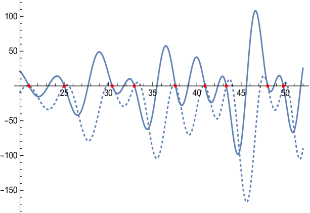
Figure 27: Bernoulli function and Riemann zeros on the critical line.

Figure 28: The Bernoulli tsunami.

Figure 29: The Bernoulli function hits Riemann’s critical line.

Figure 30:     Phase portrait of the Bernoulli function on the right half plane.

Figure 31: The Bernoulli function on the right half plane, complex view.

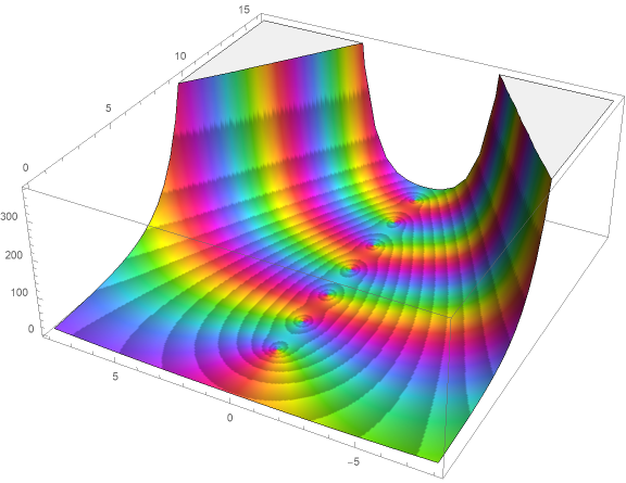
Figure 32: The Bernoulli function on the right half plane, 3-dim view.

Figure 33: The logarithm of the Bernoulli function on the right half plane.

Figure 34: The red peaks on the x-axis correspond to the real zero of the Bernoulli function (the vanishing of the odd Bernoulli numbers).

Figure 35: The front side of the plot shows the logarithm of the Bernoulli function on the critical line.

Figure 36: The Hadamard decomposition of the logarithm of the Bernoulli function as seen above is displayed in the two plots below.

Figure 37: The Hadamard decomposition of $\log\operatorname{B}:$ the Riemann $\xi$-factor.

Figure 38: The Hadamard decomposition of $\log\operatorname{B}:$ the singularity factor.

References

- [1] T. M. Apostol, Zeta and related functions, chapter 25 of the Digital Library of Mathematical Functions (DLMF), release 1.0.18 of 2018-03-27, https://dlmf.nist.gov/25.11.
- [2] D. André, Développement de and , C. R. Math. Acad. Sci. Paris (88), 965–979, (1879).
- [3] D. André, Mémoire sur les permutations alternées, J. Math. pur. appl. (7), 167–184, (1881).
- [4] T. M. Apostol, Introduction to Analytic Number Theory, Springer, 1976.
- [5] T. Arakawa, T. Ibukiyama, and M. Kaneko, Bernoulli Numbers and Zeta Functions, Springer, 2014.
- [6] I. V. Blagouchine, A theorem for the closed-form evaluation of the first generalized Stieltjes constant at rational arguments and some related summations, Journal of Number Theory, vol. 148, 537–592 and vol. 151, 276–277, (2015).
- [7] I. V. Blagouchine, Expansions of generalized Euler’s constants into the series of polynomials in and into the formal enveloping series with rational coefficients only, Journal of Number Theory, vol. 158, 365–396, (2016).
- [8] I. V. Blagouchine, Three notes on Ser’s and Hasse’s representations for the zeta-functions, Integers, Electronic Journal of Combinatorial Number Theory, vol. 18A, 1–45, (2018).
- [9] R. P. Brent and D. Harvey, Fast computation of Bernoulli, tangent and secant numbers, Computational and Analytical Mathematics, 127–142, Springer, 2013.
- [10] Boost C++ libraries, Version 1.73.0, April 2020, https://www.boost.org/doc/libs/1_73_0/libs/math/doc/html/math_toolkit/number_series/bernoulli_numbers.html.
- [11] Kwang-Wu Chen, Algorithms for Bernoulli numbers and Euler numbers, J. Integer Sequences, 4 (2001).
- [12] L. Comtet, Advanced Combinatorics, Reidel Publishing, 1974.
- [13] D. F. Connon, Some series and integrals involving the Riemann zeta function, binomial coefficients and the harmonic numbers. Volume II(b), (2007). Available at http://arxiv.org/abs/0710.4024v2.
- [14] H. M. Edwards, Riemann’s Zeta Function, Academic Press, 1974.
- [15] A. Erdélyi, W. Magnus, F. Oberhettinger, and F. Tricomi, Higher Transcendental Functions, Vol. I, 1953.
- [16] L. Euler, On the sums of series of reciprocals, §13, p. 5. Available at https://arXiv.org/abs/math.HO/0506415/
- [17] J. Franel, Note no. 245, L’Intermédiaire des mathématiciens, tome II, 153–154, (1895).
- [18] R. L. Graham, D. E. Knuth, and O. Patashnik, Concrete Mathematics: A Foundation for Computer Science, Addison-Wesley, (2nd ed.), 1994.
- [19] J. Hadamard, Étude sur les propriétés des fonctions entières et en particulier d’une fonction considérée par Riemann, Journal de Mathématiques Pures et Appliquées (58), 171–216, (1893).
- [20] P. Hadjicostas, personal communication.
- [21] H. Hasse, Ein Summierungsverfahren für die Riemannsche -Reihe, Math. Z. (32), 458–464, (1930).
- [22] J. Havil, Gamma, Exploring Euler’s Constant, Princeton University Press, (2017).
- [23] F. Hirzebruch, The signature theorem: Reminiscences and recreation, In: Prospects in mathematics. Annals of mathematics studies, (70), 3–31, (1971).
- [24] P. C. Hu and C. C. Yang, Value Distribution Theory Related to Number Theory, Birkhäuser, (2006).
- [25] J. L. W. V. Jensen, Remarques relatives aux réponses de MM. Franel et Kluyver. L’Intermédiaire des mathématiciens, tome II, Gauthier-Villars et Fils, 346–347, (1895).
- [26] F. Johansson, Rigorous high-precision computation of the Hurwitz zeta function and its derivatives, Numer Algor 69, 253–270 (2015).
- [27] F. Johansson, Arb: efficient arbitrary-precision midpoint-radius interval arithmetic, IEEE Transactions on Computers, 66(8):1281–1292, (2017).
- [28] F. Johansson and I. V. Blagouchine, Computing Stieltjes constants using complex integration, Math. of Comp., 88:318 (2019), 1829–1850.
- [29] F. Johansson, Arbitrary-precision computation of the Gamma function, Preprint hal-03346642, 2021.
- [30] E. Knobloch, H. Komatsu, D. Liu, (Eds.), Seki, Founder of Modern Mathematics in Japan, Springer Japan, (2013).
- [31] Donald E. Knuth, The Art of Computer Programming, Vol. 1: Fundamental Algorithms. 3rd edition. Addison-Wesley, (1997).
- [32] P. Luschny, The lost Bernoulli numbers, (2011), https://oeis.org/wiki/User:Peter_Luschny/TheLostBernoulliNumbers.
- [33] P. Luschny, The Bernoulli Manifesto, online since 2013, http://luschny.de/math/zeta/The-Bernoulli-Manifesto.html.
- [34] P. Luschny, Computation and asymptotics of Bernoulli numbers, (2012), http://oeis.org/wiki/User:Peter_Luschny/ComputationAndAsymptoticsOfBernoulliNumbers.
- [35] P. Luschny, Generalized Bernoulli Numbers, (2013), http://oeis.org/wiki/User:Peter_Luschny/GeneralizedBernoulliNumbers.
- [36] P. Luschny, The Swiss-Knife polynomials and Euler numbers, (2010), https://oeis.org/wiki/User:Peter_Luschny/SwissKnifePolynomials.
- [37] P. Luschny, Zeta polynomials and harmonic numbers, (2010), http://www.luschny.de/math/seq/ZetaPolynomials.htm.
- [38] P. Luschny, Eulerian polynomials, (2013), http://www.luschny.de/math/euler/EulerianPolynomials.html.
- [39] P. Luschny, Supplements for “Introduction to the Bernoulli Function”, (2020), https://github.com/PeterLuschny/BernoulliFunction.
- [40] D. Merlini, R. Sprugnoli, and M. C. Verri, The Akiyama-Tanigawa transformation, Integers (5/A05), (2005).
- [41] B. Mazur, Bernoulli numbers and the unity of mathematics, manuscript. Available at http://people.math.harvard.edu/~mazur/papers/slides.Bartlett.pdf.
- [42] G. Nemes, Generalization of Binet’s Gamma function formulas, Integral Transforms and Special Functions, 24:8, 597–606, (2013).
- [43] G. Nemes, Error bounds for the asymptotic expansion of the Hurwitz zeta function, Proceedings of the Royal Society A: Mathematical, Physical and Engineering Sciences 473, (2017).
- [44] J. Neukirch, Algebraic Number Theory, Springer, 1999.
- [45] B. Riemann, On the number of primes less than a given magnitude, (1859). Available at http://luschny.de/math/zeta/OnTheNumberOfPrimesLessThanAGivenMagnitude.html.
- [46] C. Sandifer, Some facets of Euler’s work on series. Studies in the History and Philosophy of Mathematics (5), (2007). Also in: Leonhard Euler: Life, Work and Legacy, R. E. Bradley and E. Sandifer (Ed.), Elsevier, 2007.
- [47] N. J. A. Sloane et al., The On-Line Encyclopedia of Integer Sequences, https://oeis.org, accessed in 2021.
- [48] R. P. Stanley, A survey of alternating permutations, Contemp. Math. 531, 165–196, (2010).
- [49] J. Stopple (Q), H. Cohen (A), and F. Johansson (A), On a certain integral representation for Hurwitz zeta functions, (2018), https://mathoverflow.net/questions/304965.
- [50] H. M. Srivastava, J. Choi, Series Associated with the Zeta and Related Functions, Springer, 2001.
- [51] T. Tao, Comment on: “Is Pi defined in the best way?” https://blog.computationalcomplexity.org/2007/08/is-pi-defined-in-best-way.html.
- [52] S. Vandervelde, The Worpitzky numbers revisited, The American Mathematical Monthly, 125:3, 198–206, (2018).
- [53] A. Voros, Zeta Functions over Zeros of Zeta Functions, Lecture Notes of the Unione Matematica Italiana Vol 8, 2010.
- [54] A. Weil, Number Theory: an Approach through History. From Hammurapi to Legendre, Birkhäuser, 1983.
- [55] H. S. Wilf, generatingfunctionology, Academic Press, 1990.
- [56] J. Worpitzky, Studien über die Bernoullischen und Eulerschen Zahlen, Journal für die reine und angewandte Mathematik (94), 203–232, (1883).
Index
-
alternating Bernoulli
- function An Introduction to the Bernoulli Function
- numbers An Introduction to the Bernoulli Function
- polynomials An Introduction to the Bernoulli Function
-
alternating zeta
- Hurwitz function An Introduction to the Bernoulli Function
- Riemann function An Introduction to the Bernoulli Function
-
Andre
- function Figure 20
-
André
- function An Introduction to the Bernoulli Function
- numbers An Introduction to the Bernoulli Function
- signed function An Introduction to the Bernoulli Function
- signed numbers An Introduction to the Bernoulli Function
-