Gödel Diffeomorphisms

Abstract

A basic problem in smooth dynamics is determining if a system can be distinguished from its inverse, i.e., whether a smooth diffeomorphism $T$ is isomorphic to $T^{-1}$. We show that this problem is sufficiently general that asking it for particular choices of $T$ is equivalent to the validity of well-known number theoretic conjectures including the Riemann Hypothesis and Goldbach’s conjecture. Further one can produce computable diffeomorphisms $T$ such that the question of whether $T$ is isomorphic to $T^{-1}$ is independent of ZFC.

1 Introduction

When is forward time isomorphic to backward time for a given dynamical system? When the acting group is $\mathbb{Z}$, this asks when a transformation $T$ is isomorphic to its inverse. It was not until 1951, that Anzai [2] refuted a conjecture of Halmos and von Neumann by exhibiting the first example of a transformation where $T$ is not measure theoretically isomorphic to its inverse. In fact the general problem is so complex that it cannot be be resolved using an arbitrary countable amount of information: in [11], it was shown that the collection of ergodic Lebesgue measure preserving diffeomorphisms of the 2-torus isomorphic to their inverse is complete analytic and hence not Borel.

In this paper we show that for a broad class of problems there is a one-to-one computable method of associating a Lebesgue measure preserving diffeomorphism $T_{P}$ of the two-torus to each problem $P$ in this class so that:

• $P$ is true

if and only if

• $T_{P}$ is measure theoretically isomorphic to $T_{P}^{-1}$.

The class of problems is large enough to include the Riemann Hypothesis, Goldbach’s Conjecture and statements such as “Zermelo-Frankel Set Theory ($\operatorname{\mathbf{ZFC}}$) is consistent.” In consequence, each of these problems is equivalent to the question of whether $T\cong T^{-1}$ for the diffeomorphism $T$ of 2-torus canonically associated to that problem.

Restating this, there is an ergodic diffeomorphism of the two-torus $T_{\operatorname{\mathbf{RH}}}$ such that $T_{\operatorname{\mathbf{RH}}}\cong{T_{\operatorname{\mathbf{RH}}}}^{-1}$ if and only if the Riemann Hypothesis holds, and a different, non-isomorphic ergodic diffeomorphism $T_{\operatorname{\mathbf{GC}}}$ such that $T_{\operatorname{\mathbf{GC}}}\cong{T_{\operatorname{\mathbf{GC}}}}^{-1}$ if and only if Goldbach’s conjecture holds, and so forth.

Gödel’s Second Incompleteness Theorem states that for any recursively axiomatizable theory $\Sigma$ that is sufficiently strong to prove basic arithmetic facts, if $\Sigma$ proves the statement “$\Sigma$ is consistent”, then $\Sigma$ is in fact inconsistent. The statement “$\Sigma$ is consistent” can be formalized in the manner of the problems we consider. Consider the most standard axiomatization for mathematics: Zermelo-Frankel Set Theory with the Axiom of Choice and the formalization of its consistency, the statement Con(ZFC).

If $T_{\operatorname{\mathbf{ZFC}}}$ is the diffeomorphism associated with Con(ZFC) then (assuming the consistency of conventional mathematics) the question of whether $T_{\operatorname{\mathbf{ZFC}}}\cong{T_{\operatorname{\mathbf{ZFC}}}}^{-1}$ is independent of Zermelo-Frankel Set Theory—that is, it cannot be settled with the usual assumptions of mathematics.

One can compare this with more standard independence results, the most prominent being the Continuum Hypothesis. Those independence results inherently involve comparisons between and properties of uncountable objects. The results in this paper are about the relationships between finite computable objects.

We now give precise statements of the main theorem and its corollaries. The machinery for proving these results combines ergodic theory and descriptive set theory with logical and meta-mathematical techniques originally developed by Gödel. While the statements use only standard terminology, it is combined from several fields. We have included several appendices in an attempt to convey this background to non-experts.

There are several standard references for connections between non-computable sets and analysis and PDE’s. We note one in particular with results of Marian Pour-El and Ian Richards that give an example of a wave equation with computable initial data but no computable solution [21].

1.1 The Main Theorem

As an informal guide to reading the theorem, we say a couple of words. More formal definitions appear in later sections.

• A function $F$ being computable means that there is a computer program that on input $N$ outputs $F(N)$.

• The diffeomorphisms in the paper are taken to be $C^{\infty}$ and Lebesgue measure preserving. A diffeomorphism $T$ is computable if there is a computer program that when serially fed the decimal expansions of a pair $(x,y)\in\mathbb{T}^{2}$ outputs the decimal expansions of $T(x,y)$ and for each $n$ there is a computable function computing the decimal expansion of the modulus of continuity of the $n$-th differential. Since computable functions have codes, computable diffeomorphisms also can be coded by natural numbers.

• By isomorphism, it is meant measure isomorphism. Measure preserving transformations $S:X\to X$ and $T:Y\to Y$ are measure theoretically isomorphic if there is a measure isomorphism $\varphi:X\to Y$ such that

  $$S\circ\varphi=T\circ S$$

  up to a sets of measure zero.

• In Appendix C we discuss questions such as Why $\mathbb{Z}$? Why $\mathbb{T}^{2}$? Why $C^{\infty}$?.

  We use the notation $\operatorname{Diff^{\infty}(\mathbb{T},\lambda)}$ for the collection of $C^{\infty}$ measure-preserving diffeomorphisms of $\mathbb{T}^{2}$.

• $\Pi^{0}_{1}$ statements are those number-theoretic statements that start with a block of universal quantifiers and are followed by Boolean combinations of equalities and inequalities of polynomials with natural number coefficients.

• We fix Gödel numberings: computable ways of enumerating $\Pi^{0}_{1}$ statements $\langle\varphi_{n}:n\in\mathbb{N}\rangle$ and computer programs $\langle C_{m}:m\in\mathbb{N}\rangle$. The code of $\varphi_{n}$ is $n$, the code of $C_{m}$ is $m$.

• Older literature uses the word recursive and more recent literature uses the word computable as a synonym. We use the latter in this paper. Indeed, since none of the phenomenon discussed here involve recursive behavior that is not primitive recursive we use effective, and computable as synonyms for primitive recursive.

Here is the statement of the main theorem.

Theorem 1.

(Main Theorem) There is a computable function

$$F:\{\text{Codes for $\Pi^{0}_{1}$-sentences}\}\to\{\text{Codes for computable diffeomorphisms of $\mathbb{T}^{2}$}\}$$

such that:

1. $N$ is the code for a true statement if and only if $F(N)$ is the code for $T$, where $T$ is measure theoretically isomorphic to $T^{-1}$;

2. For $M\neq N$, $F(M)$ is not isomorphic to $F(N)$.

The diffeomorphisms in the range of $F$ are Lebesgue measure preserving and ergodic.

We now explicitly draw corollaries.

Corollary 2.

There is an ergodic diffeomorphism of the two-torus $T_{\operatorname{\mathbf{RH}}}$ such that $T_{\operatorname{\mathbf{RH}}}\cong T_{\operatorname{\mathbf{RH}}}^{-1}$ if and only if the Riemann Hypothesis holds.

Similarly:

Corollary 3.

There is an ergodic diffeomorphism of the two-torus $T_{\operatorname{\mathbf{GC}}}$ such that $T_{\operatorname{\mathbf{GC}}}\cong T_{\operatorname{\mathbf{GC}}}^{-1}$ if and only if Goldbach’s Conjecture holds.

There are at least two reasons that this theorem is not trivial. The first is that the function $F$ is computable, hence the association of the diffeomorphism to the $\Pi^{0}_{1}$ statement is canonical. Secondly the function is one-to-one; $T_{\operatorname{\mathbf{RH}}}$ encodes the Riemann hypothesis and $T_{\operatorname{\mathbf{GC}}}$ encodes Goldbach’s conjecture and $T_{\operatorname{\mathbf{RH}}}\not\cong T_{\operatorname{\mathbf{GC}}}$.

Corollary 4.

Assume that $\operatorname{\mathbf{ZFC}}$ is consistent. Then there is a computable ergodic diffeomorphism $T$ of the torus such that $T$ is measure theoretically isomorphic to $T^{-1}$, but this is unprovable in Zermelo-Frankel set theory together with the Axiom of Choice.

We note again that there is nothing particularly distinctive about Zermelo-Frankel set theory with the Axiom of Choice. We choose it for the corollary because it forms the usual axiom system for mathematics. Thus Corollary 4 states an independence result in a classical form. Similar results can be drawn for theories of the form “$\operatorname{\mathbf{ZFC}}$ + there is a large cardinal” or simply ZF without the Axiom of Choice.

Finally, these results can be modified quite easily to produce diffeomorphisms of (e.g.) the unit disc with the analogous properties. Moreover techniques from the thesis of Banerjee ([4]) and Banerjee-Kunde ([3]) can be used to improve the reduction $F$ so that the range consists of real analytic maps of the 2-torus.

We finish this section by thanking Tim Carlson for asking whether Theorem 1 can be extended to lightface $\Sigma^{1}_{1}$ statements, which it can in a straightforward way. This increases the collection of statements encoded into diffeomorphisms to include virtually all standard mathematical statements.

Primitive recursion

Informally, primitive recursive functions are those that can be computed by a program that uses only for statements and not while statements. This means that the computational time can be bounded constructively using iterated exponential maps. In the statements of the results we discuss “computable functions” but in fact all of the functions constructed are primitive recursive. In particular the functions and computable diffeomorphisms asserted to exist in Theorem 1 are primitive recursive.

1.2 Hilbert’s 10th problem

Hilbert’s 10th problem asks for a general algorithm for deciding whether Diophantine equations have integer solutions. The existence of such an algorithm was shown to be impossible by a succession of results of Davis, Putnam and Robinson culminating a complete solution by Matijasevič in 1970 ([18, 6]).

Their solution can be recast as a statement very similar to Theorem 1:

There is a computable function

$$F:\{\text{Codes for $\Pi^{0}_{1}$-sentences}\}\to\{\text{Diophantine Polynomials}\}$$

such that $N$ is the code for a true statement if and only if $F(N)$ has no integer solutions.

Thus their theorem reduces general questions about the truth of $\Pi^{0}_{1}$ statements to questions about zeros of polynomials. Theorem 1 states that there is an effective reduction of the true $\Pi^{0}_{1}$ statements to $C^{\infty}$ transformations isomorphic to their inverse.

1.3 $\Pi^{0}_{1}$-sets and Gödel numberings

While the interesting corollaries of Theorem 1 are about the Riemann Hypothesis, other number theoretic statements, and independence results for dynamical systems, it is actually a theorem about subsets of $\mathbb{N}$. In order to prove it, one has to provide a way of translating between the interesting mathematical objects as they are usually constructed and the natural numbers that encode them. This is done by means of Gödel numberings, natural numbers which code the structure of familiar mathematical objects.

The arithmetization of syntax via Gödel Numbers is one of the main insights in the proofs of the Incompleteness Theorems. It is used to state “$\Sigma$ is consistent” (where $\Sigma$ is an enumerable set of axioms) as a $\Pi^{0}_{1}$ statement. Gödel numberings originally appear in [16], but are covered in any standard logic text such as [8].

The idea behind Gödel numberings is very simple: let $\langle p_{n}:n\in\mathbb{N}\rangle$ be an enumeration of the prime numbers. Associate a positive integer to each symbol: “$x$” might be 1, “$0$” might be 2, “$\forall$” might be 3 and so on. Then a sequence of symbols of length $k$ can be coded as $c=2^{n_{1}}\cdot 3^{n_{2}}\cdot 5^{n_{3}}\cdots p_{k}^{n_{k}}$.

Example 5.

Suppose we use the following coding scheme:

Symbol	x	0	$\forall$	$*$	$=$	$($	$)$
Integer	1	2	3	4	5	6	7

Then the Gödel number associated with the sentence:

$$\forall x(x*0=0)$$

is $c=2^{3}*3^{1}*5^{6}*7^{1}*11^{4}*13^{2}*17^{5}*19^{2}*23^{7}$.

Clearly the sentence can be uniquely recovered from its code. With more work, one can also use natural numbers to effectively code computer programs and their computations, sequences of formulas that constitute a proof and many other objects. The methods use the Chinese Remainder Theorem.

We now turn to $\Pi^{0}_{1}$ sentences.

Definition 6.

A sentence $\varphi$ in the language $\mathcal{L}_{\operatorname{\mathbf{PA}}}=\{+,*,0,1,<\}$ is $\Pi^{0}_{1}$ if it can be written in the form $(\forall x_{0})(\forall x_{1})\dots(\forall x_{n})\psi$, where $\psi$ is a Boolean combination of equalities and inequalities of polynomials in the variables $x_{0},\dots x_{n}$ and the constants $0,1$. (We do not allow unquantified—i.e., free—variables to appear in $\varphi$.)

It is not difficult to show that

$$\{n:\text{$n$ is the G\"{o}del number of a $\Pi^{0}_{1}$ sentence in a finite language}\}$$

is a computable set.

It is however, non-trivial to show that some statements such as the Riemann Hypothesis and the consistency of $\operatorname{\mathbf{ZFC}}$ are provably equivalent to $\Pi^{0}_{1}$-statements. The Riemann Hypothesis was shown to be $\Pi^{0}_{1}$ by Davis, Matijasevič and Robinson ([6]) and a particularly elegant version of such a statement is due to Lagarias ([17]). Appendix B.1.4 exhibits $\Pi^{0}_{1}$-statements that are equivalent to the Riemann Hypothesis (using [17]) and Goldbach’s Conjecture.

Truth:

We say a sentence $\varphi$ in the language $\mathcal{L}_{PA}$ is true if it holds in the structure $(\mathbb{N},+,*,0,1,<)$.

1.4 Effectively computable diffeomorphisms

Since $\mathbb{T}^{2}$ is compact, a $C^{\infty}$-diffeomorphism $T$ is uniformly continuous, as are its differentials. Thus, it makes sense to view their moduli of continuity as functions $d:\mathbb{N}\to\mathbb{N}$ which say, informally, that if one wishes to specify the map $(x,y)\mapsto T(x,y)$ to within $2^{-n}$, then the original point $(x,y)$ must be specified to within a tolerance of $2^{-d(n)}$. With better and better information about $(x,y)$, one can produce better and better information about $T(x,y)$. This intuitive notion is formalized by the definitions given below, and in more detail in Appendix B.2.2. We note in passing that the moduli of continuity and approximations are not uniquely defined.

Definition 7 (Effective Uniform Continuity).

We say that a map $T:\mathbb{T}^{2}\to\mathbb{T}^{2}$ is effectively uniformly continuous if and only if the following two computable functions exist:

• A computable Modulus of Continuity: A computable function $d:\mathbb{N}\to\mathbb{N}$ which, given a target accuracy $\epsilon$ finds the $\delta$ within which the source must be known to approximate the function within $\epsilon$.

  More concretely, suppose $T:[0,1)\times[0,1)\to[0,1)\times[0,1)$. View elements in $[0,1)$ as their binary expansions. Then the first $d(n)$ digits of each of $(x,y)$ determine the first $n$ digits of the two entries of $T(x,y)$.

• A Computable Approximation: A computable function $f:(\{0,1\}\times\{0,1\})^{<\mathbb{N}}\to(\{0,1\}\times\{0,1\})^{<\mathbb{N}}$, which, given the first $d(n)$ digits of the binary expansion of $(x,y)$—or, equivalently, the dyadic rational numbers $(k_{x}\cdot 2^{-d(n)},k_{y}\cdot 2^{-d(n)})$ for $0\leq k_{x},k_{y}\leq 2^{d(n)}$ closest to $(x,y)$— outputs the first $n$ digits of the binary expansion of the coordinates of $T(x,y)$.

The diffeomorphisms $T$ we build are $C^{\infty}$ and map from $\mathbb{T}^{2}$ to $\mathbb{T}^{2}$. Because we are working on $\mathbb{T}^{2}$ we can view $T$ as a map from $\mathbb{R}^{2}$ to $\mathbb{R}^{2}$. The $k^{th}$ differential is determined by the collection of $k^{th}$ partial derivatives $\{{\partial^{k}\over\partial^{i}x\partial^{k-i}y}:0\leq i\leq k\}$ of $T$ with respect to the standard coordinate system for $\mathbb{R}^{2}$. For $k<\infty$, $T$ is effectively $C^{k}$ provided that for each $n<k$ there are computable $d(n,-)$ and $f(n,-)$ that give the moduli of continuity and approximations to the partial $n^{th}$ derivatives. Being $C^{\infty}$ requires that the $d(n,-)$ and $f(n,-)$ exist and are uniformly computable; that is that there is a single algorithm that on every input $n\in\mathbb{N}$ computes $d(n,-)$ and $f(n,-)$.

For clarity, in these definitions we discussed functions with domain and range $\mathbb{T}^{2}$. There is no difficulty generalizing effective uniform continuity to effectively presented metric spaces. The notion of a computable $C^{k}$ diffeomorphism also easily generalized to smooth manifolds $M$ and their diffeomorphisms, using atlases.

We note that computable diffeomorphisms are uniquely determined by the procedures for computing $d$ and $f$ and hence they too may be coded using Gödel numbers. The elements of the range of the function $F$ in Theorem 1 code diffeomorphisms in this manner.

Inverses of recursive diffeomorphisms

It is not true that the inverse of a primitive recursive function $f:\mathbb{N}\to\mathbb{N}$ is primitive recursive. However for primitive recursive diffeomorphisms of compact manifolds it is. Suppose that $M$ is a smooth compact manifold and $T$ is a $C^{\infty}$-diffeomorphism. Then $T$ is a diffeomorphism and hence has uniformly Lipschitz differentials of all orders. Since $T$ is invertible and $M$ is compact, $T^{-1}$ also has uniformly Lipschitz differentials of all orders. Moreover the Lipschitz constants for $T^{-1}$ are “one over” the Lipschitz constants for $T$. It follows in a straightforward way that the inverse of a primitive recursive diffeomorphism on $M$ is a primitive recursive diffeomorphism.

1.5 Reductions

The key idea for proving Theorem 1 is that of a reduction.

Definition 8.

Suppose that $A\subseteq X$ and $B\subseteq Y$ and $f:X\to Y$. Then $f$ reduces $A$ to $B$ if

$$x\in A\mbox{ iff }f(x)\in B.$$

The idea behind a reduction is that to determine whether a point $x$ belongs to $A$ one looks at $f(x)$ and asks whether it belongs to $B$: $f$ reduces the question “$x\in A$” to “$f(x)\in B$.

For this to be interesting the function $f$ must be relatively simple. In many cases the spaces $X$ and $Y$ are Polish spaces and $f$ is taken to be a Borel map. In this paper $X=Y=\mathbb{N}$ and $F$ is primitive recursive.

In [11] the function $f$ has domain the space of trees (equivalently, acyclic countable graphs) and has range the space of measure preserving diffeomorphisms of the two-torus. It reduces the collection of ill-founded trees (those with an infinite branch or, respectively, acyclic graphs with a non-trivial end) to diffeomorphisms isomorphic to their inverse.

The function $f$ is a Borel map. The point there is that if $\{T:T\cong T^{-1}\}$ were Borel then its inverse by the Borel function $f$ would also have to be Borel. But the set of ill-founded trees is known not to be Borel. Hence the isomorphism relation of diffeomorphisms is not Borel.

In the current context the function $F$ in Theorem 1 maps from a computable subset of $\mathbb{N}$ (the collection of Gödel numbers of $\Pi^{0}_{1}$ statements) to $\mathbb{N}$. It takes values in the collection of codes for diffeomorphisms of the two-torus.

Theorem 1 can be restated as saying that $F$ is a primitive recursive reduction of the collection $A$ of Gödel numbers for true $\Pi^{0}_{1}$ statements to the collection $B$ of codes for computable measure preserving diffeomorphisms of the torus that are isomorphic to their inverses. For $N\neq M$ the transformation $F(N)$ is not isomorphic to $F(M)$.

Thus Theorem 1 can be restated as saying that the collection of true $\Pi^{0}_{1}$ statements is computably reducible to the collection of measure preserving diffeomorphisms that are isomorphic to their inverses. In the jargon: the collection of diffeomorphisms isomorphic to their inverses is “$\Pi^{0}_{1}$-hard.”

1.6 Structure of the paper

The proof of the main theorem in this paper depends on background in two subjects, requiring the quotation of key results that would be prohibitive to prove. The actual construction itself—that is, the reduction $F$ of the main theorem—is described in its entirety, along with the intuition behind these results.

The paper heavily uses results proved in [9], [11], [12] and [13]. When used, the results are quoted, and informal intuition is given for the proofs. When specific numbered lemmas, theorems and equations from [11] are referred to, the numbers correspond to the arXiv version cited in the bibliography.

Structure of the paper

The logical background required for the proof of Theorem 1 is minimal and the exposition is aimed at an audience with a basic working knowledge of ergodic theory, in particular the Anosov-Katok method.

Section 2 defines the odometer-based transformations, a large class of measure preserving symbolic systems. These are built by iteratively concatenating words without spacers. We then construct the reduction $F_{\mathcal{O}}$ from the true $\Pi^{0}_{1}$ statements to the ergodic odometer-based transformations isomorphic to their inverse.

Section 3 moves from symbolic dynamics to smooth dynamics. This proceeds in two steps. The first step is to define a class of symbolic systems, the circular systems that are realizable as measure preserving diffeomorphisms of the two-torus. The second step uses the Global Structure Theorem of [12], which shows that the category whose objects are odometer-based systems and whose morphisms are synchronous and anti-synchronous joinings is canonically isomorphic with the category whose objects are circular systems and whose objects are synchronous and anti-synchronous joinings. Thus the odometer-based systems in the range of $F_{\mathcal{O}}$ can be canonically associated with symbolic shifts that are isomorphic to diffeomorphisms.

Section 3.2 shows that different elements of the range of $\mathcal{F}\circ F_{\mathcal{O}}$ are not isomorphic, by showing that their Kronecker factors are different. Sections 3.3 discusses diffeomorphisms of the torus and how to realize circular systems using method of Approximation by Conjugacy due to Anosov and Katok. Section 3.3 builds a primitive recursive map $R$ from circular construction sequences to measure preserving diffeomorphisms of $\mathbb{T}^{2}$ such that ${\mathbb{K}}^{c}\cong R({\mathbb{K}}^{c})$.

In section 3.4 we argue that the functor $\mathcal{F}$ defined in the Global Structure Theorem is itself a reduction when composed with $F_{\mathcal{O}}$. Hence composing $R$, $\mathcal{F}$ and $F_{\mathcal{O}}$ gives a reduction $F$ from the collection of true $\Pi^{0}_{1}$ statements to the collection of ergodic diffeomorphisms of the torus that are isomorphic to their inverse. This completes the proof of Theorem 1.

The overall content of the paper is summarized by Figure 1. The reduction to odometer-based systems is $F_{\mathcal{O}}$, $\mathcal{F}$ is the functorial isomorphism, the realization as smooth transformations is $R$ and the composition $F$ is the reduction in Theorem 1.

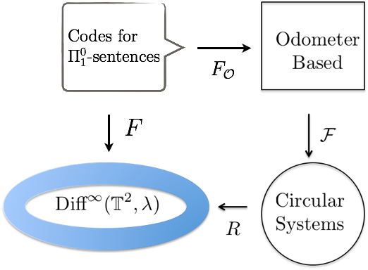
Figure 1: The reduction $F$.

The Appendix

In the course of the proof of Theorem 1 various numerical parameters are chosen with complex relationships. The are collected, explicated and shown to be coherent in Appendix A.

Sections 2 and 3 of the body of the paper use certain standard notions and constructions in ergodic theory and computability theory. A complete presentation is impossible, but for readers who want an general overview we present basic ideas from each subject as well exhibit explicit formulations of certain techniques used in the paper.

Appendix B is an overview of the logical background necessary for the proof of the theorem. It includes a basic description of $\Pi^{0}_{1}$ formulas, a discussion of bounded quantifiers, how to express Goldbach’s conjecture as a $\Pi^{0}_{1}$ formula and the definition of “truth.” Appendix B.2 gives basic background on recursion theory, computable functions, and primitive recursion. Appendices B.2.2 and B.2.3 give background on effectively computable functions.

Appendix C gives background about ergodic theory and measure theory. It includes the notion of a measurable dynamical system, the Koopman operator, and the ergodic theorem. Appendix C.3 describes symbolic systems and gives the notation and basic definitions and conventions used in this paper. Appendix C.4 gives basic facts about odometers and odometer-based systems. These include the eigenvalues of the Koopman Operator associated to an odometer transformation and the canonical odometer factor associated with an odometer-based system. Appendix C.5 gives basic definitions including the relationship between joinings and isomorphisms. It discusses disintegrations and relatively independent products.

Appendix D gives basic definitions of the space of $C^{\infty}$ diffeomorphisms and gives an explicit construction of a smooth measure preserving near-transposition of adjacent rectangles. The latter is a tool used in constructing the smooth permutations of subrectangles of the unit square. These permutations are the basic building blocks of the approximations to the diffeomorphisms in the reduction. The section verifies that these are recursive diffeomorphisms with recursive moduli of continuity and that they can be given primitively recursively.

Gaebler’s Theorem

The writing of this paper began as a collaboration between J. Gaebler and the author with the goal of recording Foreman’s results establishing Theorem 1. Mathematically, Gaebler was concerned with understanding the foundational significance of Theorem 1. Though unable to finish this writing project, Gaebler established the following theorem in Reverse Mathematics:

Theorem (Gaebler’s Theorem).

Theorem 1 can be proven in the system ACA₀.

This result will appear in a future paper [14].

Acknowledgements

The author has benefited from conversations with a large number of people. These include J. Avigad, T. Carlson, S. Friedman, M. Magidor, A. Nies, T.  Slaman (who pointed out the analogy with Hilbert’s 10th problem), J. Steel, H. Towsner, B. Velickovic and others. B. Kra was generous with suggestions for the emphases of the paper and with help editing the introduction. B. Weiss, was always available and as helpful as usual. Finally my colleague A. Gorodetski was indispensable for providing suggestions about how to edit the paper to make it more accessible to dynamicists.

2 Odometer-Based Systems and Reductions

In this section we prove the existence of the preliminary reduction $F_{\mathcal{O}}$.

Theorem 9.

There is a primitive recursive function $F_{\mathcal{O}}$ from the codes for $\Pi^{0}_{1}$-sentences to primitive recursive construction sequences for ergodic odometer based transformations such that:

1. $N$ is the code for a true statement if and only if $F_{\mathcal{O}}(N)$ is the code for a construction sequence with limit $T$, where $T$ is measure theoretically isomorphic to $T^{-1}$.

2. For $M\neq N$, $F_{\mathcal{O}}(M)$ is not isomorphic to $F_{\mathcal{O}}(N)$.

Remark 10.

When discussing the construction of $F_{\mathcal{O}}$ and $F$ we will always have the unstated assumption that the input $N$ is a Gödel number of a $\Pi^{0}_{1}$-statement.

This is justified by remarking that, though formally the domain of $F_{\mathcal{O}}$ (and so of $F$) is the collection of $N$ that are Gödel numbers of $\Pi^{0}_{1}$-statements, the collection of Gödel numbers of $\Pi^{0}_{1}$-statements is primitive recursive. Theorem 1 is equivalent to asking that $F$ be defined on all of $\mathbb{N}$ and output a code for the identity map when the input is an $N$ that is not a Gödel number of a $\Pi^{0}_{1}$-statement.

2.1 Basic Definitions

Both Odometer Based and Circular symbolic systems are built using construction sequences, a tool we now describe. They code cut-and-stack constructions and give a collection of words that constitute a clopen basis for the support of an invariant measure.

Fix a non-empty alphabet $\Sigma$. If $\mathcal{W}$ is a collection of words in $\Sigma$, we will say that $\mathcal{W}$ is uniquely readable if and only if whenever $u,v,w\in\mathcal{W}$ and $uv=pws$ then either:

• $p=\emptyset$ and $u=w$ or

• $s=\emptyset$ and $v=w$.

A consequence of unique readability is that an arbitrary infinite concatenation of words from $\mathcal{W}$ can be uniquely parsed into elements of $\mathcal{W}$.

Fix an alphabet $\Sigma$. A Construction Sequence is a sequence of collections of uniquely readable words $\langle\mathcal{W}_{n}:n\in\mathbb{N}\rangle$ with the properties that:

1. Each word in $\mathcal{W}_{n}$ is in the alphabet $\Sigma$.

2. For each $n$ all of the words in $\mathcal{W}_{n}$ have the same length $q_{n}$. The number of words in $\mathcal{W}_{n}$ will be denoted $s_{n}$.

3. Each $w\in\mathcal{W}_{n}$ occurs at least once as a subword of every $w^{\prime}\in\mathcal{W}_{n+1}$.

4. There is a summable sequence $\langle\epsilon_{n}:n\in\mathbb{N}\rangle$ of positive numbers such that for each $n$, every word $w\in\mathcal{W}_{n+1}$ can be uniquely parsed into segments

   $$u_{0}w_{0}u_{1}w_{1}\dots w_{l}u_{l+1}$$ (1)

   such that each $w_{i}\in\mathcal{W}_{n}$, $u_{i}\in\Sigma^{<\mathbb{N}}$ and for this parsing

   $$\frac{\sum_{i}|u_{i}|}{q_{n+1}}<\epsilon_{n+1}.$$ (2)

The segments $u_{i}$ in condition 1 are called the spacer or boundary portions of $w$. The uniqueness requirement in clause 3 implies unique readability of each word in every $\mathcal{W}_{n}$.

Let ${\mathbb{K}}$ be the collection of $x\in\Sigma^{\mathbb{Z}}$ such that every finite contiguous subword of $x$ occurs inside some $w\in\mathcal{W}_{n}$. Then ${\mathbb{K}}$ is a closed shift-invariant subset of $\Sigma^{\mathbb{Z}}$ that is compact if $\Sigma$ is finite. The symbolic shift $({\mathbb{K}},sh)$ will be called the limit of $\langle\mathcal{W}_{n}:n\in\mathbb{N}\rangle$.

Definition 11.

Let $f\in{\mathbb{K}}$ where ${\mathbb{K}}$ is built from a construction sequence $\langle\mathcal{W}_{n}:n\in\mathbb{N}\rangle$. Then by unique readability, for all $n$ there is a unique $w\in\mathcal{W}_{n}$ and $a_{n}\leq 0<b_{n}$ such that $f\mathbin{\upharpoonright}[a_{n},b_{n})\in\mathcal{W}_{n}$. This $w$ is called the principal $n$-subword of $f$. If the principal $n$-subword of $f$ lies on $[a_{n},b_{n})$ we define $r_{n}(f)=-a_{n}$, the location of $f(0)$ relative to the interval $[a_{n},b_{n})$.

The construction sequences built in this paper are strongly uniform in that for each $n$ there is a number $f_{n}$ such that each word $w\in\mathcal{W}_{n}$ occurs exactly $f_{n}$ times in each word $w^{\prime}\in\mathcal{W}_{n+1}$. It follows that $({\mathbb{K}},sh)$ is uniquely ergodic.

We note that in definition 11 we must have $b_{n}-a_{n}=q_{n}$.

Notation

For a word $w\in\Sigma^{<\mathbb{N}}$ we will write $|w|$ for the length of $w$.

Inverses and reversals

If ${\mathbb{K}}$ is a symbolic shift built from a construction sequence $\langle\mathcal{W}_{n}:n\in\mathbb{N}\rangle$ then we can consider its inverse in two ways. The first is $({\mathbb{K}},\operatorname{\textsc{Sh}}^{-1})$. The second, which we call $\textsc{Rev}({{\mathbb{K}}})$ is the system built from the construction sequence $\langle\textsc{Rev}({\mathcal{W}_{n}}):n\in\mathbb{N}\rangle$ where $\textsc{Rev}({\mathcal{W}_{n}})$ is the collection of reversed words from $\mathcal{W}_{n}$: if $w\in\mathcal{W}_{n}$ then $w$ written backwards belongs to $\textsc{Rev}({\mathcal{W}_{n}})$. Clearly $({\mathbb{K}},\operatorname{\textsc{Sh}}^{-1})$ is isomorphic to $(\textsc{Rev}({{\mathbb{K}}}),sh)$ and we will use both conventions depending on context.

Odometer Based construction sequences

A construction sequence with $\mathcal{W}_{0}=\Sigma$ and built without spacers is called an odometer-based construction sequence. For odometer-based sequences, Clause 3 of the definition of Construction Sequence implies that for odometer based systems $\mathcal{W}_{n+1}\subseteq\mathcal{W}_{n}^{k_{n}}$ for some sequence $\langle k_{n}:n\in\mathbb{N}\rangle$ of natural numbers with $k_{n}\geq 2$. Hence $|\mathcal{W}_{n+1}|\leq|\mathcal{W}_{n}|^{k_{n}}$. In the special case of odometer sequences we write the length of words in $\mathcal{W}_{n}$ as $K_{n}$. We note that $K_{n}=\prod_{m=0}^{n-1}k_{m}$.

The sequence $\langle k_{n}:n\in\mathbb{N}\rangle$ determines an odometer transformation with domain the compact space

$$\boldmath{O}=_{def}\prod_{n}\mathbb{Z}_{k_{n}}.$$

The space $\boldmath O$ is naturally a monothetic compact abelian group. We will denote the group element $(1,0,0,0,\dots)$ by $\bar{1}$, and the result of adding $\bar{1}$ to itself $j$ times by $\bar{j}$. There is a natural map of $\boldmath O$ given by $\mathcal{O}(x)=x+\bar{1}$. Then $\mathcal{O}$ is a topologically minimal, uniquely ergodic invertible homeomorphism of $\boldmath O$ that preserves Haar measure. The map $x\mapsto-x$ is an isomorphism of $\mathcal{O}$ with $\mathcal{O}^{-1}$. (See Appendix C.4 and [9] for more background.)

Odometer transformations are characterized by their Koopman operators. They are discrete spectrum and the group of eigenvalues is generated by the $K_{n}$-th roots of unity.

The odometer factor

If ${\mathbb{K}}$ is built from an odometer-based construction sequence and the principal $n$-subword of $f$ sits at $[-a_{n},b_{n})$ then the sequence $\langle a_{n}:n\in\mathbb{N}\rangle$ gives a well defined member $\pi_{\mathcal{O}}(f)$ of $\boldmath O=\prod_{i}\mathbb{Z}_{k_{i}}$. It is easy to verify that the map $f\mapsto\pi_{\mathcal{O}}(f)$ is a factor map.

A measure preserving transformation is odometer-based if it is finite entropy, ergodic and has an odometer factor. It is shown in [10] that every odometer-based transformation is isomorphic to a symbolic shift with an odometer-based construction sequence.

2.2 Inverses and factors induced by equivalence relations

Fix an odometer based construction sequence $\langle\mathcal{W}_{n}:n\in\mathbb{N}\rangle$. If $\mathcal{Q}$ is an equivalence relation on $\mathcal{W}_{n}$, then elements of ${\mathbb{K}}$ can be viewed as determining sequences of equivalence classes. More precisely if $\Sigma^{*}$ is the alphabet consisting of classes $\mathcal{W}_{n}/\mathcal{Q}$ we can consider the collection $\mathcal{W}_{n}^{*}$ of words of length $K_{n}$ that are constantly equal to an element of $\Sigma^{*}$. Let $m>n$. Then for some $K$, the words in $\mathcal{W}_{m}$ are concatenations of $K$-words from $\mathcal{W}_{n}$. Viewed this way, the words in $\mathcal{W}_{m}$ determine a sequence of $K$ many elements of $\mathcal{W}_{n}^{*}$. Concatenating them we get a word of length $K_{m}$ that is constant on contiguous blocks of length $K_{n}$. Let $\mathcal{W}_{m}^{*}$ be the collection of words in the alphabet $\Sigma^{*}$ arising this way. There is a clear projection map $\pi:\mathcal{W}_{m}\to\mathcal{W}_{m}^{*}$ that sends two words in $\mathcal{W}_{m}$ to the same word in $\mathcal{W}_{m}^{*}$ if they induce the same sequence of $\mathcal{Q}$-classes.

Equivalently define the diagonal equivalence relation $\mathcal{Q}^{K}$ on $\mathcal{W}_{n}^{K}$ by setting

$$w_{0}w_{1}\dots w_{K-1}\sim w^{\prime}_{0}w^{\prime}_{1}\dots w^{\prime}_{K-1}$$

if and only if for all $i,w_{i}\sim_{\mathcal{Q}}w^{\prime}_{i}$. Then for two words $w,w^{\prime}\in\mathcal{W}_{m},\pi(w)=\pi(w^{\prime})$ if and only if $w\sim_{\mathcal{Q}^{K}}w^{\prime}$. Similarly let $w\in{(\mathcal{W}_{n}/Q)}^{K}$ and $w^{\prime}\in\mathcal{W}_{m}^{K}$. Then $w^{\prime}$ is a substitution instance of $w$ if and only if

$$w^{\prime}=w_{0}w_{1}\cdots w_{K-1}\ \text{and}\ w=[w_{0}]_{Q}[w_{1}]_{Q}\cdots[w_{K-1}]_{Q}.$$

The sequence $\langle\mathcal{W}_{m}^{*}:m\geq n\rangle$ determines a well-defined odometer-based construction sequence in the alphabet $\Sigma^{*}$. If we define ${\mathbb{K}}_{\mathcal{Q}}$ to be the limit of $\langle\mathcal{W}_{m}^{*}:m\geq n\rangle$ then there is a canonical factor map $\pi_{\mathcal{Q}}:{\mathbb{K}}\to{\mathbb{K}}_{\mathcal{Q}}$.

We now discuss how this factor map behaves with inverse transformation. Suppose that $\mathbb{Z}_{2}$ acts freely on $\Sigma^{*}=\mathcal{W}_{n}/\mathcal{Q}$. Then for all $K$ we can extend this action to $(\Sigma^{*})^{K}$ by the skew-diagonal action. Suppose that $g$ is the generator of $\mathbb{Z}_{2}$. Define

$$g\cdot([w_{0}]_{\mathcal{Q}}[w_{1}]_{\mathcal{Q}}\dots[w_{K-1}]_{\mathcal{Q}})=g\cdot[w_{K-1}]_{\mathcal{Q}}g\cdot[w_{K-2}]\dots g\cdot[w_{0}].$$

Assume that $\mathcal{W}_{m}^{*}$ is closed under the skew-diagonal action. Let

$$w=[w_{0}][w_{1}][w_{K-1}]\in\mathcal{W}_{m}^{*}.$$

Then we can apply $g$ pointwise to the $[w_{i}]$; i.e. the diagonal action. Since $\mathcal{W}_{m}^{*}$ is closed under the skew-diagonal action, the word $g[w_{0}]g[w_{1}]\dots g[w_{K-1}]\in\textsc{Rev}({\mathcal{W}_{m}^{*}})$.

Lemma 12.

Suppose for all $m>n,\mathcal{W}_{m}^{*}$ is closed under the skew-diagonal action of $g$. Then ${\mathbb{K}}_{\mathcal{Q}}\cong\textsc{Rev}({{\mathbb{K}}_{\mathcal{Q}}})$ and the isomorphism takes an $f\in{\mathbb{K}}_{\mathcal{Q}}$ with associated odometer sequence $x$ to an element of $\textsc{Rev}({{\mathbb{K}}_{\mathcal{Q}}})$ determined by the diagonal action that has associated odometer sequence $-x$.

$\vdash$   The sequence $\langle\textsc{Rev}({\mathcal{W}_{m}^{*}}):m\geq n\rangle$ is a construction sequence for $\textsc{Rev}({{\mathbb{K}}_{\mathcal{Q}}})$. The map

$$[w_{0}][w_{1}]\dots[w_{K-1}]\mapsto g[w_{0}]g[w_{1}]\dots g[w_{K-1}]\in\textsc{Rev}({\mathcal{W}_{m}^{*}})$$

is an invertible shift-equivariant map defined on the construction sequences for ${\mathbb{K}}_{\mathcal{Q}}$ and $\textsc{Rev}({{\mathbb{K}}_{\mathcal{Q}}})$ and hence defines an invertible graph joining $\eta_{g}$ from ${\mathbb{K}}_{\mathcal{Q}}$ to $\textsc{Rev}({{\mathbb{K}}_{\mathcal{Q}}})$ $\dashv$

We note that the graph joining $\eta_{g}$ does not depend on which elements of $\mathcal{W}_{n}$ are identified by $\mathcal{Q}$. Moreover to recover $\textsc{Rev}({{\mathbb{K}}})$ from $\textsc{Rev}({{\mathbb{K}}_{\mathcal{Q}}})$ one substitutes the appropriate reverse words $\textsc{Rev}({w})$ into a $\mathcal{Q}$-class ${\mathcal{C}}$. Frequently the graph joining $\eta_{g}$ of ${\mathbb{K}}_{\mathcal{Q}}$ with $\textsc{Rev}({{\mathbb{K}}_{\mathcal{Q}}})$ does not come from a graph joining of ${\mathbb{K}}$ with $\textsc{Rev}({{\mathbb{K}}})$.

In the construction in [9], which we modify in this paper, this process is iterated: there is an equivalence relation $\mathcal{Q}_{1}$ on $\mathcal{W}_{n_{1}}$ and another equivalence relation $\mathcal{Q}_{2}$ on $\mathcal{W}_{n_{2}}$ with $n_{1}<n_{2}$ and $\mathcal{Q}_{2}$ a refinement of the product equivalence relation $\mathcal{Q}_{1}^{K}$ (for the appropriate $K$). There will be two copies of $\mathbb{Z}_{2}$ generated by $g_{1}$ and $g_{2}$ with $g_{1}$ acting freely on $\mathcal{W}_{n_{1}}/\mathcal{Q}_{1}$ and $g_{2}$ acting freely on $\mathcal{W}_{n_{2}}/\mathcal{Q}_{2}$.

For $i=1,2$ denote $\mathcal{W}_{m}/(\mathcal{Q}_{i})^{K}$ by $(\mathcal{W}_{m}^{*})_{i}$. We build two construction sequences consisting of collections of words made up of equivalence classes $\langle(\mathcal{W}^{*}_{m})_{1}:m\geq n_{1}\rangle$ and $\langle(\mathcal{W}^{*}_{m})_{2}:m\geq n_{2}\rangle$ which we assume are closed under the skew-diagonal actions of $g_{1}$ and $g_{2}$ respectively. Let ${\mathbb{K}}_{1}$ be the limit of $\langle(\mathcal{W}^{*}_{m})_{1}:m\geq n_{1}\rangle$ and ${\mathbb{K}}_{2}$ the limit of $\langle(\mathcal{W}^{*}_{m})_{2}:m\geq n_{2}\rangle$.

Then we get a tower

$$\begin{diagram}$$

Suppose the $g_{2}$ action on $\mathcal{Q}_{2}$ is subordinate to the $g_{1}$ action on $\mathcal{W}_{n_{2}}/(\mathcal{Q}_{1})^{K}$; that is, whenever ${\mathcal{C}}_{1}$ and ${\mathcal{C}}_{2}$ are classes of $\mathcal{W}_{n_{2}}/(\mathcal{Q}_{1})^{K}$ and $\mathcal{W}_{n_{2}}/\mathcal{Q}_{2}$ and ${\mathcal{C}}_{2}\subseteq{\mathcal{C}}_{1}$, then $g_{2}{\mathcal{C}}_{2}\subseteq g_{1}{\mathcal{C}}_{1}$.

Then the various projection maps between ${\mathbb{K}}$, ${\mathbb{K}}_{\mathcal{Q}_{2}}$ and ${\mathbb{K}}_{\mathcal{Q}_{1}}$ commute with the shift and the joining $\eta_{g_{2}}$ of ${\mathbb{K}}_{\mathcal{Q}_{2}}\times\textsc{Rev}({{\mathbb{K}}_{\mathcal{Q}_{2}}})$ extends the joining $\eta_{g_{1}}$ of ${\mathbb{K}}_{\mathcal{Q}_{1}}\times\textsc{Rev}({{\mathbb{K}}_{\mathcal{Q}_{1}}})$. Given an infinite sequence of equivalence relations $\mathcal{Q}_{i}$, the associated joinings cohere into an invertible graph joining of ${\mathbb{K}}$ with $\textsc{Rev}({{\mathbb{K}}})$ if and only if the $\sigma$-algebras associated with the ${\mathbb{K}}_{\mathcal{Q}_{i}}$ generate the measure algebra on ${\mathbb{K}}$.

Diagonal vs Skew-diagonal actions.

Since $\curvearrowright_{n}$ extends to both the diagonal and skew-diagonal actions, we summarize the distinct rolls:

• The skew-diagonal actions give closure properties on $\mathcal{W}_{m}/\mathcal{Q}^{m}_{n}=(\mathcal{W}_{m}^{*})_{n}$ .

• Because of this closure the diagonal action gives an isomorphism between ${\mathbb{K}}_{n}$ and $\textsc{Rev}({{\mathbb{K}}})_{n}$. This approximates a potential isomorphism from ${\mathbb{K}}$ to $\textsc{Rev}({{\mathbb{K}}})$.

2.3 Elements of the construction

The construction of the first reduction $F_{\mathcal{O}}$ closely parallels the construction in [9] and we refer the reader to that paper for details of claims made here. For each $N$ the routine $F_{\mathcal{O}}(N)$ inductively builds an odometer construction sequence $\langle\mathcal{W}_{n}:n\in\mathbb{N}\rangle$ in the alphabet $\Sigma=\{0,1\}$ with $\mathcal{W}_{n+1}\subseteq\mathcal{W}_{n}^{k_{n}}$. During the construction we will accumulate inductive numerical requirements. Some, such as the $\epsilon_{n}$’s and the $\varepsilon_{n}$’s are positive numbers that go to zero rapidly. Some, such as the $k_{n}$’s and $l_{n}$’s are sequences of natural numbers that go to infinity. These numbers depend on $N$, so when necessary we will write $\mathcal{W}_{n}(N)$, $\epsilon_{n}(N)$, $k_{n}(N)$, $l_{n}(N)$ and so forth. However for notational simplicity we will drop the $N$ whenever it is clear from context. At stage $n$ in the algorithm $F(N)$ for building $\mathcal{W}_{n}(N)$, for $M<N$ $F$ can recursively refer to objects build by $F(M)$ at stages $\leq n$. For example $F(N)$ can assume that $k_{n}(N-1)$ is known.

These sequences of numbers are defined inductively and have complex relationships, requiring some verification that they are consistent and can be chosen primitively recursively. That they are consistent is the content of section 10 of [11]. That they can be chosen primitively recursively involves a routine review of the arguments in that paper. For completeness this is done in Appendix A.

Numerical Requirement A

$s_{n}=2^{(n+1)e(n-1)}$ for an increasing sequence of natural numbers $e(n)$.

The construction will use the following auxiliary objects and their properties:

1. A sequence of equivalence relations $\langle\mathcal{Q}_{n}:1\leq n<\infty\rangle$. Each $\mathcal{Q}_{n}$ is an equivalence relation on $\mathcal{W}_{n}$, hence gives a factor ${\mathbb{K}}_{n}$ of ${\mathbb{K}}$.

2. The equivalence relation $\mathcal{Q}_{n+1}$ refines the product equivalence relation $(\mathcal{Q}_{n})^{k_{n}}$ on $\mathcal{W}_{n}^{k_{n}}$.

3. The sub-$\sigma$-algebra $\mathcal{H}_{n}$ of $\mathcal{B}({\mathbb{K}})$ corresponding to ${\mathbb{K}}_{n}$. In the construction here, as with the original construction, $\bigcup_{n}\mathcal{H}_{n}$ will generate $\mathcal{B}({\mathbb{K}})$ modulo the sets of measure zero with respect to the unique shift-invariant measure $\mu$. (This is Lemma 14 which uses specification Q4.)

   We denote the sub-$\sigma$-algebra of $\mathcal{B}({\mathbb{K}})$ corresponding to the odometer fact by $\mathcal{H}_{0}$. Because the odometer factor sits in side each ${\mathbb{K}}_{n}$, $\mathcal{H}_{0}\subseteq\mathcal{H}_{n}$ for all $n$.

4. A system of free $\mathbb{Z}_{2}$ actions $\curvearrowright_{n}$ on $\mathcal{W}_{n}/\mathcal{Q}_{n}$ for $n<\Omega$. Denote the generator of $\mathbb{Z}_{2}$ corresponding to $\curvearrowright_{n}$ as $g_{n}$.

Suppose that $n<m$. As in section 2.2, the words in $\mathcal{W}_{m}$ are concatenations of $K=K_{m}/K_{n}$-many words from $\mathcal{W}_{n}$. Hence the product equivalence relation $(\mathcal{Q}_{n})^{K}$ gives an equivalence relation on $\mathcal{W}_{m}$, which we call $\mathcal{Q}^{m}_{n}$. We will denote $\mathcal{W}_{m}/\mathcal{Q}^{m}_{n}$ by $(\mathcal{W}_{m}^{*})_{n}$. The $\mathbb{Z}_{2}$ actions have the following properties:

• $(\mathcal{W}_{m}^{*})_{n}$ is closed under the skew-diagonal action of $g_{n}$.

• If $n+1<\Omega$, then the $g_{n+1}$ action is subordinate to the $g_{n}$ action.

• We let $\curvearrowright_{n}$ be the diagonal action of $g_{n}$ on ${\mathbb{K}}_{n}$. Since $(\mathcal{W}_{m}^{*})_{n}$ is closed under the skew-diagonal action, $\curvearrowright_{n}$ can be viewed as mapping $(\mathcal{W}_{m}^{*})_{n}$ to $\textsc{Rev}({(\mathcal{W}_{m}^{*})_{n}})$. As described in section 2.2, for $n<\Omega$, $\curvearrowright_{n}$ canonically creates an isomorphism between ${\mathbb{K}}_{n}$ and ${\mathbb{K}}_{n}^{-1}$ that induces the map $x\mapsto-x$ on the odometer factor.

Restating this: if the action $\curvearrowright_{n}$ is non-trivial, then it induces a graph joining $\eta_{n}$ of $\mathcal{H}_{n}$ with $(\mathcal{H}_{n})^{-1}$ that projects to the map $x\mapsto-x$ on the odometer factor. Assuming $n+1<\Omega$, the action $\curvearrowright_{n+1}$ is subordinate to $\curvearrowright_{n}$, the joining $\eta_{n+1}$ projects to the joining $\eta_{n}$. If $\Omega=\infty$, since the $\bigcup_{n}\mathcal{H}_{n}$ will generate $\mathcal{B}({\mathbb{K}})$, the $\eta_{n}$’s will consequently cohere into a conjugacy of $T$ with $T^{-1}$.

Lemmas 26 and 27 of [9] formalize this and show the following conclusion.

Lemma 13.

Suppose $\Omega=\infty$. Then there is a measure isomorphism $\eta$ of ${\mathbb{K}}$ with ${\mathbb{K}}^{-1}$ such that for all $n\in\mathbb{N}$, $\eta$ induces an isomorphism $\eta_{n}:{\mathbb{K}}_{n}\to{\mathbb{K}}_{n}$ that coincides with the graph joining determined by the action of the generator for $\curvearrowright_{n}$ on ${\mathbb{K}}_{n}$.

The construction is arranged so that if the number $\Omega$ in clause 3 of the description of the objects is finite, then ${\mathbb{K}}\not\cong{\mathbb{K}}^{-1}$. This is done by making the sequences of equivalence classes of elements of $(\mathcal{W}_{m}^{*})_{n}=\mathcal{W}_{m}/\mathcal{Q}^{m}_{n}$ essentially independent of their reversals subject to the conditions described above. The specifications given later in this section make this precise.

2.4 An overview of $F_{\mathcal{O}}$.

The algorithm for the reduction $F_{\mathcal{O}}$ is diagrammed in Figure 2.

Figure 2: The algorithm $R_{\varphi}=F_{\mathcal{O}}(N)$.

Given $N$, $F_{\mathcal{O}}$ determines the $\Pi^{0}_{1}$ formula coded by $N$:

$$\varphi_{N}=\forall z_{0}\forall z_{1}\dots\forall z_{m}\varphi(z_{0},z_{1},\dots z_{m}).$$

The function $F$ then uses the formula to generate a computational routine $R_{\varphi}$ that recursively computes the objects $\mathcal{W}_{n}(N),\mathcal{Q}_{n}(N)$ and $\curvearrowright_{n}\!(N)$ (as well as the various numerical parameters that are involved in the construction). Here is what $R_{\varphi}$ does.

The routine $R_{\varphi}$

1. Fixes a computable enumeration of all $m$-tuples $\langle\vec{z}_{n}=(z_{0},\dots z_{m})_{n}:n\in\mathbb{N}\rangle$ of natural numbers

2. On input $n$, $R_{\varphi}$ initializes $i=0$, sets $\mathcal{W}_{0}=\{0,1\}$, $\mathcal{Q}_{0}$ the trivial equivalence relation with one class and the action $\curvearrowright_{0}$ the trivial action.

3. For $i<n$, $R_{\varphi}$:

   1. builds $\mathcal{W}_{i+1},\mathcal{Q}_{i+1}$,

   2. computes $\langle\vec{z}_{j}:0\leq j\leq i\rangle$,

   3. Asks:

      “Is $$\varphi_{N}(\vec{z}_{j}) 0\leq j\leq i$$ true for all ?”

      Since $\varphi_{N}$ has no unbounded quantifiers, this question is primitive recursive.

   4. If yes, $R_{\varphi}$ builds the action $\curvearrowright_{i+1}$

   5. If no, $R_{\varphi}$ makes the $\curvearrowright_{i+1}$ trivial. (Note that if $i$ is the first integer in this case, then $\Omega$ will equal $i+1$.)

4. When $i=n$, $R_{\varphi}$ returns $\mathcal{W}_{n}$.

2.5 Properties of the words and actions.

We describe the construction sequence, the equivalence relations and the actions. To start we choose a prime number $P_{0}>2$ sufficiently large, and let $\langle P_{N}:N>0\rangle$ enumerate the prime numbers bigger than $P_{0}$.

For the construction sequence corresponding to $F_{\mathcal{O}}(N)$, words in $\mathcal{W}_{1}$ have length $P_{N}$. The words in $\mathcal{W}_{n}$ will have length ${K_{n}=P_{N}2^{\ell}}$ for some $\ell$ chosen large enough as specified below. The $K_{n}$’s will be increasing and $K_{m}$ divides $K_{n}$ for $m<n$. Let $k_{n}=K_{n+1}/K_{n}$. Thus $k_{n}$ is a large power of 2 and each word in $\mathcal{W}_{n+1}$ is a concatenation of $k_{n}$ many words from $\mathcal{W}_{n}$. The number of words in $\mathcal{W}_{n}$ is $s_{n}$. We require that $s_{n}$ divides $s_{n+1}$ and $s_{n}$ is a power of 2 that goes to goes to infinity quickly. Since $\mathcal{W}_{n+1}\subseteq\mathcal{W}_{n}^{k_{n}}$ this induces lower bounds on the growth of the $k_{n}$’s.

The requirements described here are simpler than those in [9] as modified in [11], and the “specifications” used there are appropriately simplified or omitted if not relevant to this proof. The construction carries along numerical parameters $\langle\epsilon_{n}\rangle$, $\langle k_{n}\rangle$, $\langle K_{n}\rangle$, $\langle s_{n}\rangle$, $\langle Q_{n}\rangle$, $\langle C_{n}\rangle$, and $\langle e(n)\rangle$. (Showing that the various coefficients are compatible and primitively recursively computable appears in Appends A.)

As an aid to the reader we use the analogous labels for the simplified specifications as those that appear in [11].

Q4

For $n\geq 1$, any two $\mathcal{W}_{n}$-words in the same $\mathcal{Q}_{n}$ class agree on an initial segment of proportion at least $(1-\epsilon_{n})$.

Q6.

As a relation on $\mathcal{W}_{n+1}$, for $1\leq s\leq n+1$, $\mathcal{Q}^{n+1}_{s}$ refines $\mathcal{Q}^{n+1}_{s-1}$ and each $\mathcal{Q}^{n}_{s-1}$ class contains $2^{e(n)}$ many $\mathcal{Q}^{n}_{s}$ classes.

The point of Q4 is that the $\mathcal{Q}_{n}$ classes approximate words in $\mathcal{W}_{n}$ by specifying arbitrarily long proportions of the words. A consequence of this is:

Lemma 14.

$\bigcup_{n}\mathcal{H}_{n}$ generates the measure algebra of ${\mathbb{K}}$.

$\vdash$   This is proved in Proposition 23 of [9]. $\dashv$

Thus Q4 is the justification for Assertion 3 of Section 2.3.

We now turn to the joining specifications. These are counting requirements that determine the joining structure. The joining specifications we present here are more complicated than strictly necessary for the simplified construction in this paper, but we present them as appear in [9] in order to be able to directly quote the theorems proved there. We note that specification J10.1 is a strengthening of J10 in [9].

Suppose that $u$ and $v$ are elements of $\mathcal{W}_{n+1}\cup\textsc{Rev}({\mathcal{W}_{n+1}})$ and $(u^{\prime},v^{\prime})$ an ordered pair from $\mathcal{W}_{n}\cup\textsc{Rev}({\mathcal{W}_{n}})$. Suppose that $u$ and $v$ are in positions shifted relative to each other by $t$ units. Then an occurrence of $(u^{\prime},v^{\prime})$ in $(sh^{t}(u),v)$ is a $t^{\prime}$ such that $u^{\prime}$ occurs in $u$ starting at $t+t^{\prime}$ and in $v$ starting at $t^{\prime}$. If $X$ is an alphabet and $\mathcal{W}$ is a collection of words in $X$, and $u\in\mathcal{W}\cup\textsc{Rev}({\mathcal{W}})$ we say that $u$ has forward parity if $u\in\mathcal{W}$ and reverse parity if $u\in\textsc{Rev}({\mathcal{W}})$.

By specification Q4 no word in $\mathcal{W}_{n+1}$ belongs to $\textsc{Rev}({\mathcal{W}_{n+1}})$, so parity is well-defined and unique. However the words in $(\mathcal{W}^{*}_{n})_{i}$ may belong to $\textsc{Rev}({(\mathcal{W}^{*}_{n})_{i}})$ and we view those words as having both parities.

J10.1

Let $u$ and $v$ be elements of $\mathcal{W}_{n+1}\cup\textsc{Rev}({\mathcal{W}_{n+1}})$. Let $1\leq t<(1-\epsilon_{n})(k_{n})$. Let $j_{0}$ be a number between $\epsilon_{n}k_{n}$ and $k_{n}-t$. Then for each pair $u^{\prime},v^{\prime}\in\mathcal{W}_{n}\cup\textsc{Rev}({\mathcal{W}_{n}})$ such that $u^{\prime}$ has the same parity as $u$ and $v^{\prime}$ has the same parity as $v$, let $r(u^{\prime},v^{\prime})$ be the number of $j<j_{0}$ such that $(u^{\prime},v^{\prime})$ occurs in $(sh^{tK_{n}}(u),v)$ in the $j\cdot K_{n}$-th position in their overlap. Then

$$\left|\frac{r(u^{\prime},v^{\prime})}{j_{0}}-\frac{1}{s_{n}^{2}}\right|<\epsilon_{n}.$$

For fixed $n$ and $s$, let $Q^{n}_{s}=|(\mathcal{W}^{*}_{n})_{s}|$ and $C^{n}_{s}$ be the number of equivalent elements in each block of the partition $\mathcal{W}_{n}/\mathcal{Q}^{n}_{s}$.

J11

Suppose that $u\in\mathcal{W}_{n+1}$ and $v\in\mathcal{W}_{n+1}\cup\textsc{Rev}({\mathcal{W}_{n+1}})$. We let $s=s(u,v)$ be the maximal $i<\Omega$ such that $[u]_{i}$ and $[v]_{i}$ are in the same $\curvearrowright_{i}$-orbit. Let $g=g_{i}$ and $(u^{\prime},v^{\prime})\in\mathcal{W}_{n}\times(\mathcal{W}_{n}\cup\textsc{Rev}({\mathcal{W}_{n}}))$ be such that $g[u^{\prime}]_{s}=[v^{\prime}]_{s}$. Let $r(u^{\prime},v^{\prime})$ be the number of occurrences of $(u^{\prime},v^{\prime})$ in $(u,v)$. Then:

$$\left|\frac{r(u^{\prime},v^{\prime})}{k_{n}}-\frac{1}{Q^{n}_{s}}\left(\frac{1}{C^{n}_{s}}\right)^{2}\right|<\epsilon_{n}.$$

The next assumption is a strengthening of a special case of J11.

J11.1

Suppose that $u\in\mathcal{W}_{n+1}$ and $v\in\mathcal{W}_{n+1}\cup\textsc{Rev}({\mathcal{W}_{n+1}})$ and $[u]_{1}$ not in the $\curvearrowright_{1}$-orbit of $[v]_{1}$. Let $j_{0}$ be a number between $\epsilon_{n}k_{n}$ and $k_{n}$. Suppose that $I$ is either an initial or a tail segment of the interval $\{0,1,\dots K_{n+1}-1\}$ having length $j_{0}K_{n}$. Then for each pair $u^{\prime},v^{\prime}\in\mathcal{W}_{n}\cup\textsc{Rev}({\mathcal{W}_{n}})$ such that $u^{\prime}$ has the same parity as $u$ and $v^{\prime}$ has the same parity as $v$, let $r(u^{\prime},v^{\prime})$ be the number of occurrences of $(u^{\prime},v^{\prime})$ in $(u\mathbin{\upharpoonright}I,v\mathbin{\upharpoonright}I)$. Then:

$$\left|\frac{r(u^{\prime},v^{\prime})}{j_{0}}-\frac{1}{s_{n}^{2}}\right|<\epsilon_{n}.$$

The properties and specifications described above imply the specifications in [9] as well as J10.1 and J11.1 from [11].

Remark 15.

We note that specification J10.1 implies unique readability of the words in $\mathcal{W}_{n+1}$. This follows by induction on $n$. If the words in $\mathcal{W}_{n+1}$ were not uniquely readable then we would have $u,v,w\in\mathcal{W}_{n}$ with $uv=pws$ and neither $p$ nor $s$ empty. But the one of $u$ or $v$ would have to overlap either an initial segment or a tail segment of $w$ of length $K_{n+1}/2$. Suppose it is an initial segment of $w$ and a tail segment $u$. On this tail segment the $n$-subwords would have to agree exactly with the $n$-subwords of an initial segment of $w$. But this contradicts $J10.1$.

Suppose we have built a collection of words $\langle\mathcal{W}_{n}:n\in\mathbb{N}\rangle$, equivalence relations $\langle\mathcal{Q}_{n}:n\in\mathbb{N}\rangle$ and actions $\langle\curvearrowright_{n}:n\in\mathbb{N}\rangle$ satisfying the properties described then we can cite the following results occurring in [9]. Fix a transformation $T$ built with the construction sequence $\langle\mathcal{W}_{n}:n\in\mathbb{N}\rangle$. Recall that if $\curvearrowright_{n}$ is non-trivial then the generator $g_{n}\neq 0$ induces an invertible graph joining $\eta_{n}$ of ${\mathbb{K}}_{n}$ with ${\mathbb{K}}_{n}^{-1}$. We quote the following results of [9], referencing their numbers in that paper.

Theorem 13 and Proposition 32

Suppose that $\eta$ is an ergodic joining of $T$ with $T^{-1}$ that is not a relatively independent joining over the odometer factor. Then $\eta\mathbin{\upharpoonright}\mathcal{H}_{0}\times\mathcal{H}_{0}$ is supported on the graph of some $\bar{j}$-shift of the odometer factor.

Proposition 37

If $\eta$ is an ergodic joining of ${\mathbb{K}}$ with ${\mathbb{K}}^{-1}$, then exactly one of the following holds:

1. $\Omega<\infty$ and for some $n\leq\Omega$, $j\in\mathbb{Z}$ and some $\eta_{n}$, $\eta$ is the relatively independent joining of ${\mathbb{K}}$ with ${\mathbb{K}}^{-1}$ over the joining $\eta_{n}\circ(1,sh^{-j})$ of ${\mathbb{K}}_{n}\times{\mathbb{K}}_{n}^{-1}$.

2. $\Omega=\infty$ and for some $j$, all $n$ the projection of $\eta$ to a joining on ${\mathbb{K}}_{n}\times{\mathbb{K}}_{n}^{-1}$ is of the form $\eta_{n}\circ(1,sh^{-j})$

If $\Omega=\infty$, since the $\mathcal{H}_{n}$’s generate, $\eta$ is an invertible graph joining of ${\mathbb{K}}$ with ${\mathbb{K}}^{-1}$. In both cases the projection of $\eta_{n}$ to a joining of the odometer factor with itself concentrates on the map $x\mapsto-x$.

Thus it follows that:

1. If ${\mathbb{K}}\cong{\mathbb{K}}^{-1}$ then $\Omega=\infty.$ In particular if ${\mathbb{K}}\cong{\mathbb{K}}^{-1}$, then the $\Pi^{0}_{1}$ statement $\varphi_{N}$ is true.

2. The projection of $\eta_{n}\circ(1,sh^{-j})$ to the odometer is of the form $x\mapsto-x-j$.

3. Similarly the projection of $\eta\circ(1,sh^{-j})$ to the odometer is of the form $x\mapsto-x-j$.

Clause 2 of Theorem 9 requires that if $M\neq N$ are different codes for $\Pi^{0}_{1}$ sentences then the transformation $F_{\mathcal{O}}(M)$ is not isomorphic to $F_{\mathcal{O}}(N)$. This is clear because the odometer sequence for $F_{\mathcal{O}}(M)$ consists of $k$’s whose prime factors are $2$ and $P_{M}$, while the odometer sequence for $F_{\mathcal{O}}(N)$ has $k$’s whose prime factors are $2$ and $P_{N}$. Since $P_{M}\neq P_{M}$, the odometer factors are not isomorphic.

Corollary 33 of [9] implies that the Kronecker factor of each $F_{\mathcal{O}}(N)$ is the odometer factor. Since any isomorphism $\varphi$ between $F_{\mathcal{O}}(M)$ with $F_{\mathcal{O}}(N)$ must induce an isomorphism of the Kronecker factors, $\varphi$ has to induce an isomorphism of the corresponding odometer factors, yielding a contradiction. (See Corollary 57 in Appendix C)

To finish the proof of Theorem 9 we must show that the words, equivalence relations and actions can be built primitively recursively.

2.6 Building the words, equivalence relations and actions

To finish the proof of Theorem 9 the words $\mathcal{W}_{n}(N)$, the equivalence relations $\mathcal{Q}_{n}(N)$ and actions $\curvearrowright_{n}(N)$ must be constructed and it must be verified that the construction is primitive recursive.

Note:

Formally we are just constructing actions $\curvearrowright_{n}$ for $n<\Omega$. However for notational convenience, when constructing the words at stage $n+1$, we will write $\curvearrowright_{i}$ when $\Omega\leq i<n+1$ with the understanding that it is the trivial identity action.

The collections of words $\mathcal{W}_{n}$ are built probabilistically. A finitary version of law of large numbers shows that there are primitive recursive bounds on the length of the words in a collection with the necessary properties. The actual collection of words can then be found with an exhaustive search of collections of words of that length, showing that the entire construction is primitive recursive.

Structure of the induction.

The collections of words $\mathcal{W}_{n}$ are built by induction on $n$. For $n\geq 1$ the words in $\mathcal{W}_{n+1}$ are built by iteratively substituting words into $k_{n}$-sequences of classes $\mathcal{Q}_{i}^{n}$, by induction on $i\leq n$. We will adapt the notation of section 2.2.

The length $K_{1}$ of words in $\mathcal{W}_{1}$ will be a large prime number $P_{N}$. To pass from stage $n$ to $n+1$, one is required to build the words $\mathcal{W}_{n+1}$, the equivalence relation $\mathcal{Q}_{n+1}$ and, if $n+1<\Omega$ the action $\curvearrowright_{n+1}$. The length $K_{n+1}$ of the words will be ${2^{\ell}\cdot K_{n}}$ for an $\ell$ taken large enough.

Suppose we have already chosen $k_{n}$ and it is a large power of 2. Then $(\mathcal{Q}^{n}_{i})^{k_{n}}$ for $0\leq i\leq n$ give us a hierarchy of equivalence relations of potential words as described in Section 2.2 as well as the diagonal and skew-diagonal actions of $\curvearrowright_{i}$ for $i<\min(n,\Omega)$.

Remark 16.

The construction of $\mathcal{W}_{n+1}$ is top-down. We construct the $(\mathcal{W}^{*}_{n+1})_{i}=\mathcal{W}_{n+1}/\mathcal{Q}^{n+1}_{i}$ by induction on $i$ before we construct $\mathcal{W}_{n+1}$. The equivalence relations get more refined as $i$ increases, so each step gives more information about $\mathcal{W}_{n+1}$. Having built $(\mathcal{W}^{*}_{n+1})_{n}$, an additional step constructs creates $\mathcal{W}_{n+1}$ and the equivalence relation $\mathcal{Q}^{n+1}_{n+1}$.

Start with $i=0$. Then $\mathcal{W}_{n}/\mathcal{Q}^{n}_{0}$ has one element, a string of length $K_{n}$ with a single letter. Let $(\mathcal{W}_{n+1}^{*})_{0}$ be the single element consisting of strings of length $k_{n}\cdot K_{n}$ in that single letter.

Each element of $(\mathcal{W}^{*}_{n+1})_{1}$ is built by substituting $k_{n}$ elements of $(\mathcal{W}_{n}^{*})_{1}$—each of which is a contiguous block of length $K_{n}$—into $(\mathcal{W}_{n+1}^{*})_{0}$. We continue this process inductively, ultimately arriving at $(\mathcal{W}^{*}_{n+1})_{n}$.

The elements $X$ being substituted	The result of the substitution
into previous words
	$(\mathcal{W}_{n+1}^{*})_{0}$
$(\mathcal{W}_{n}^{*})_{1}$	$(\mathcal{W}_{n+1}^{*})_{1}$
$(\mathcal{W}_{n}^{*})_{2}$	$(\mathcal{W}_{n+1}^{*})_{2}$
⋮	⋮
$(\mathcal{W}_{n}^{*})_{n}$	$(\mathcal{W}_{n+1}^{*})_{n}$

The result of this induction is a sequence of elements of $\mathcal{W}_{n}/\mathcal{Q}_{n}$ of length $k_{n}*K_{n}$, that is constant on blocks of length $K_{n}$. We must finish by substituting elements of $\mathcal{W}_{n}$ into the $\mathcal{W}_{n}/\mathcal{Q}_{n}$-classes to get $\mathcal{W}_{n+1}$ and defining $\mathcal{Q}_{n+1}$.

A step in the induction on $i$.

Fix an $i$ and view elements $(\mathcal{W}_{n+1}^{*})_{i}$ as $k_{n}$-sequences $C_{0}C_{1}\dots C_{k_{n}-1}$ of elements of $(\mathcal{W}^{*}_{n})_{i}$. Since $\mathcal{Q}_{i+1}$ refines the diagonal equivalence relation $(\mathcal{Q}_{i})^{K_{i+1}/K_{i}}$, $(\mathcal{Q}_{i+1}^{n})^{k_{n}}$ refines $(\mathcal{Q}_{i}^{n})^{k_{n}}$. Inside each $\mathcal{Q}^{n}_{i}$ class $C_{j}$, one can choose a $\mathcal{Q}^{n}_{i+1}$ class $C^{\prime}_{j}\in(\mathcal{W}_{n}^{*})_{i+1}$ . Concatenating these to get $C_{0}^{\prime}C_{1}^{\prime}\dots C_{k_{n}-1}^{\prime}$ we create an element of $(\mathcal{W}^{*}_{n+1})_{i+1}$. We do the construction so that result is closed under the skew diagonal action of $\curvearrowright_{i+1}$.

Remark 17.

Following section 2.2, elements of $(\mathcal{W}_{i+1}^{*})_{i+1}$ are constant sequences of length $K_{i+1}$. Thus the concatenation $C_{0}^{\prime}C_{1}^{\prime}\dots C_{k_{n}-1}^{\prime}$ is a sequence of $k_{n}*(K_{n}/K_{i+1})$ many contiguous constant blocks of length $K_{i+1}$.

We now describe how these choices are made. Our discussion is aimed at the case where $n+1<\Omega$, for $n+1\geq\Omega$ take $\curvearrowright_{n+1}$ to be the trivial action. Fix a candidate $k$ for $k_{n}$. View $\{rev\}$ as acting on $(\mathcal{W}_{n}/\mathcal{Q}_{i}^{n})^{k}=((\mathcal{W}_{n}^{*})_{i})^{k}$. Together, the skew-diagonal action of $\curvearrowright_{i}$ and $\{rev\}$ generate an action on $(\mathcal{W}_{n}/\mathcal{Q}_{i}^{n})^{k}$. Let $R_{i}$ be a set of representatives of each orbit of this action. Fix the number $E$ of $i+1$-classes desired inside each $i$-class. Consider

$$\mathbb{X}_{i}=\prod_{r\in R_{i}}\prod_{q=0}^{E-1}S(r,q),$$ (3)

where $S(r,q)$ is the collection of all substitution instances of $\mathcal{Q}^{n}_{i+1}$ classes into $r$. More explicitly, if $r=C_{0}C_{2}\dots C_{k-1}$ where $C_{j}\in\mathcal{W}_{n}/\mathcal{Q}^{n}_{i}$. Let $C_{j}^{*}=\{C^{\prime}:C^{\prime}\subseteq C_{j}\mbox{ and }C^{\prime}\in\mathcal{W}_{n}/\mathcal{Q}^{n}_{i+1}\}$. For each $0\leq q\leq E-1$, let

$$S(r,q)=\prod_{j=0}^{k-1}C_{j}^{*}.$$

Fix an $r\in R_{i}$. The every element $\mathcal{W}$ of $\prod_{q=0}^{E-1}S(r,q)$ can be viewed as a collection of $E$ many words of length $k$ in the language $(\mathcal{W}_{n}^{*})_{i+1}$ whose $\mathcal{Q}_{i}^{n}$ classes form $r$. Each of these $E$ many words can be copied by the $\curvearrowright_{i+1}$ action. If $w$ is such a word, and is a substitution instance of $r$ then $\curvearrowright_{i+1}(w)$ is a substitution instance of $\curvearrowright_{i}(r)$.

So comparing elements of $\mathcal{W}$ (and their shifts) is the same as comparing potential words in $(\mathcal{W}_{n+1}^{*})_{i+1}$. The action of $\curvearrowright_{i+1}$ preserves the frequencies of occurrences of words in

We work with $\mathbb{X}_{i}$ because it can be viewed as a discrete measure space with the counting measure. The objects being counted in the various specifications correspond to random variables on this measure space.

Definition 18.

If $\langle w_{r,q}:r\in R_{i},0\leq q<E\rangle$ is the collection of words built using the Substitution Lemma passing from stage $i$ to stage $i+1$, the $(\mathcal{W}^{*}_{n+1})_{i+1}$ is the closure of $\{w_{r,q}:r\in R_{i},0\leq q<E\}$ under the skew-diagonal action of $\curvearrowright_{i}$.

Example 19.

If $C\subseteq C_{j},D\subseteq C_{j^{\prime}}$ are substitution instances, we have the independent random variables $X_{r,q,j},X_{r^{\prime},q^{\prime},j^{\prime}}$ taking value 1 at points $\vec{x}\in\mathbb{X}_{i}$ where $x(r,q,j)=C$ and $x(r^{\prime},q^{\prime},j^{\prime})=D$, respectively. The event that $C$ occurs in $\mathbb{X}_{i}$ in the $q^{th}$ word in position $j$ and $D$ occurs in $r^{\prime}$ in the $(q^{\prime})^{th}$ word in position $j^{\prime}$ is the event that both $X_{r^{\prime},q^{\prime},j^{\prime}}=1$ and $X_{{r,q,j}}=1$. If each $i$-class has $p$ elements then the probability that both $X_{r^{\prime},q^{\prime},j^{\prime}}=1$ and $X_{{r,q,j}}=1$ is $1/p^{2}$.

The strong law of large numbers tells us that the collection of points in each $\mathbb{X}_{i}$ that do not satisfy the specifications (as they are coded in the conclusion of the Substitution Lemma) goes to zero exponentially fast in $k$. As $k$ grows, the number of requirements to satisfy the Substitution Lemma grows linearly. Hoeffding’s inequality (Theorem 21 below) says that the probabilities stabilize exponentially fast. The Substitution Lemma follows.

In more detail:

The word construction proceeds by first getting a very close approximation to what is desired and then finishing the approximations to exactly satisfy the requirements. These two steps correspond to Proposition 43 and Lemma 41 of [9].

The general setup for the Substitution Lemma (Proposition 20) at stage $n+1$ is as follows:

• An alphabet $X$ and an equivalence relation $\mathcal{Q}$ on $X$, with $Q$ classes each of cardinality $C$.

• A collection of words $\mathcal{W}\subseteq(X/\mathcal{Q})^{k}$ for some $k$.

• Groups $G,H$ with generators $g,h$ that are either $\mathbb{Z}_{2}$ or the trivial group. If $H=\mathbb{Z}_{2}$ then $G=\mathbb{Z}_{2}$.

• If $G=\mathbb{Z}_{2}$ then we have a free action $G\curvearrowright X/Q$ and if $H=\mathbb{Z}_{2}$ we also have a free action $H\curvearrowright X$. Thus the skew-diagonal actions of $G$ on $(X/Q)^{k}$ and $H$ on $X^{k}$ are well-defined. If either group is trivial, then the corresponding actions are trivial.

• The $H\curvearrowright X$ action is subordinate to $G\curvearrowright X/Q$ action via $\rho$.

• Constants $\epsilon_{a},\epsilon_{b}\in(0,1)$ such that $\epsilon_{b}<\epsilon_{a}^{2}/5|X|$.

• A constant $E$ determining the number of substitution instances desired for each $\mathcal{Q}$ class.

• If $u,v,w,w^{\prime}$ are words in the alphabet $X$, then $r(u,v,sh^{i}(w),w^{\prime})$ is the number of $j$ such that $u$ occurs in $w$ starting at $j+i$ and $v$ occurs in $w^{\prime}$ starting at $j$. Similarly if $u,w$ are words in the alphabet $X$, the $r(u,w)$ is the number of occurrences of $u$ in $w$.

A special case of the Substitution Lemma (Proposition 63 in [9]) is:

Proposition 20 (Substitution Lemma).

Let $E>0$ be an even number. There is a lower bound $\mathit{k}_{\textsc{lb}}$ depending on $(\epsilon_{b},\epsilon_{a},Q,C,W,E)$ such that for all numbers $k\geq\mathit{k}_{\textsc{lb}}$ and all symmetric $\mathcal{W}\subseteq{(X/\mathcal{Q})^{k}}$ with cardinality $W$ that are closed under the skew-diagonal action of $G$ and $\textsc{Rev}({})$, if for all $i$ with $1\leq i\leq(1-\epsilon_{b})k$, $u,v\in X/\mathcal{Q}$ and $w,w^{\prime}\in\mathcal{W}$:

$$\left|\frac{r(u,v,sh^{i}(w),w^{\prime})}{k-i}-\frac{1}{Q^{2}}\right|<\epsilon_{b}$$ (4)

and each $u\in X/\mathcal{Q}$ occurs with frequency $1/Q$ in each $w\in\mathcal{W}$,

then there is a collection of words $S\subseteq{X}^{k}$ consisting of substitution instances of $\mathcal{W}^{k}$ such that if $\mathcal{W}^{\prime}=HS\cup\textsc{Rev}({HS})$ we have:

1. Every element of $\mathcal{W}^{\prime}$ is a substitution instance of an element of $\mathcal{W}$ and each element of $\mathcal{W}$ has exactly $E$ many substitution instances of words in $\mathcal{W}^{\prime}$.

2. For each $x\in X$ and each $w\in\mathcal{W}^{\prime}$

   $$\left|\frac{r(x,w)}{k}-\frac{1}{|X|}\right|<\epsilon_{a}$$ (5)

   i.e., the frequency of $x$ in $w$ is within $\epsilon_{a}$ of $1/|X|$.

3. If $w_{1},w_{2}\in S\cup\textsc{Rev}({S})$ with $[w_{1}]_{\mathcal{Q}}=[w_{2}]_{\mathcal{Q}}$ and $w_{2}\notin H_{0}w_{1}$ and $x,y\in X$ with $[x]=[y]$. Then for $h\in H_{0}$:

   $$\left|\frac{r(x,y,w_{1},hw_{2})}{k}-\frac{1}{Q\cdot C^{2}}\right|<\epsilon_{a}.$$ (6)

4. Let $i$ be a number with $1\leq i\leq(1-\epsilon_{a})k$ and $j_{0}$ be a number between $\epsilon_{a}k/2$ and $k-i$, $x,y\in X$, $w_{1},w_{2}\in\mathcal{W}^{\prime}\cup\textsc{Rev}({\mathcal{W}^{\prime}})$, let $r(x,y)$ be the number of $j<j_{0}$ such that $(x,y)$ occurs in $(sh^{i}(w_{1}),w_{2})$ in the $j^{th}$ position. Then

   $$\left|\frac{r(x,y)}{j_{0}}-\frac{1}{|X|^{2}}\right|<\epsilon_{a}.$$ (7)

5. For all $x,y\in X$ and all $w_{1},w_{2}\in\mathcal{W}^{\prime}\cup\textsc{Rev}({\mathcal{W}^{\prime}})$ with different $H$ orbits,

   $$\left|\frac{r([x]_{\mathcal{Q}},[y]_{\mathcal{Q}},[w_{1}]_{\mathcal{Q}},[w_{2}]_{\mathcal{Q}})}{k}-c\right|<\epsilon_{b}$$ (8)

   implies that,

   $$\left|\frac{r(x,y,w_{1},w_{2})}{k}-\frac{c}{C^{2}}\right|<\epsilon_{a}.$$ (9)

We remark again that the Law of Large numbers implies that conclusions 1-5 hold for almost all infinite sequences. For example if you perform i.i.d. substitutions of elements of $X$ to create a typical infinite sequence $\vec{w}$, then the density of occurrences of a given $x$ in $\vec{w}$ will be $1/|x|$. The Hoeffding inequality says that the finitary approximations to this conclusion converge exponentially fast. As a result, for large enough $k$ it is possible to satisfy conclusions 1-5 with very high probability.

Another remark is that at each stage we start with a collection of words $\mathcal{W}$ closed under reversals and produce another collection of words $\mathcal{W}^{\prime}$ closed under reversals.

The sequence $e(n)$.

We will have a sequence $e(n)$ such that for $n\geq 1$, $s_{n+1}=2^{(n+2)e(n)}$ that satisfies some growth conditions. (See Inherited Requirement 2 and Inherited Requirement 3 in Appendix A and Figure 5 for an explicit statement of these conditions.) To initialize the construction we take $e(0)=2$.

Finding $k_{n}$

We now use Proposition 20 to build the collections of words. We will apply it with $E=2^{e(n)}$ except in one instance where we apply it with $E=2^{2e(n)}$. To start the inductive construction, we take $P_{0}$ to be large enough to apply the Substitution Lemma $\mathcal{Q}_{0}$ the trivial equivalence relation and $\mathcal{W}_{0}=\Sigma=\{0,1\}$. For $N>0$, since $P_{N}\geq P_{0}$, $P_{N}$ can also be used for $k_{0}(N)$ to initialize the construction as described below with $n=0$.

We then choose $k_{n}$ large enough to allow $n+1$ successive Lemma 20-style substitutions for $E=2^{2e(n)}$ corresponding to the equivalence relations $\mathcal{Q}^{n}_{i}$ for $1\leq i\leq n$ together with a final substitution of the letters in the base alphabet $\Sigma$ to produce $\mathcal{W}_{n+1}$. (This is a total of $n+2$ substitutions.)

More explicitly, note that each of the $n+2$ applications of the Substitution Lemma for the various $\mathcal{Q}_{i}$ with $E=2^{2e(n)}$ and $\epsilon_{a}=\epsilon_{n}/100$ and the finishing lemma produces a lower bound $\mathit{k}_{\textsc{lb}}^{i}$.

The following will be important later in the paper:

Numerical Requirement B

Let $k_{n}(N-1)$ be the $k_{n}$ corresponding to the reduction $F_{\mathcal{O}}(N-1)$ and $k_{n}(N)$ be the $k_{n}$ corresponding to the reduction $F_{\mathcal{O}}(N)$ and $k_{n}(N)$. Then

$$k_{n}(N)\geq k_{n}(N-1)$$ (10)

Choose a large power of two

$$\mathit{k}_{\textsc{Max}}>\max\{\mathit{k}_{\textsc{lb}}^{0},\mathit{k}_{\textsc{lb}}^{1},\ldots,\mathit{k}_{\textsc{lb}}^{n},k_{n}(N-1)\},$$

ensuring that it be sufficiently large that $2^{-\mathit{k}_{\textsc{Max}}}<\epsilon_{n}$. Then, set

$$k_{n}=\mathit{k}_{\textsc{Max}}^{2}*s_{n}.$$ (11)

Since $k_{n}$ is of this form and $s_{n}$ is a power of 2, this ensures that $K_{n+1}=P_{N}\cdot 2^{\ell}$ for a large $\ell$. By increasing $\mathit{k}_{\textsc{Max}}$ if necessary we can also assume

1. $1/k_{n}<\epsilon^{3}_{n}/4$.

2. $s_{n+1}\leq s_{n}^{k_{n}}$.

Building $\mathcal{W}_{n+1}/\mathcal{Q}_{i}^{n+1}$ for $i\leq n$:

This is done by applying the Substitution Lemma $n$ times to pass from $(\mathcal{W}^{*}_{n+1})_{0}$ successively to $(\mathcal{W}^{*}_{n+1})_{n}$. At each $i<n$ we substitute $2^{e(n)}$ many elements of $(\mathcal{W}^{*}_{n+1})_{i+1}$ into each element of $(\mathcal{W}^{*}_{n+1})_{i}$.

Completing $\mathcal{W}_{n+1}$:

Having constructed $\mathcal{W}_{n+1}/\mathcal{Q}_{n}$ it remains to construct $\mathcal{W}_{n+1}$, $\mathcal{Q}_{n+1}$ and the action $\curvearrowright_{n+1}$. The latter is only relevant if $n+1<\Omega$.

We must ensure that the resulting collection of words satisfy Q4 and Q6. This is accomplished by constructing two collections of words, the stems and the tails.

Start by rewriting $\mathit{k}_{\textsc{Max}}^{2}$ as $(\mathit{k}_{\textsc{Max}}^{2}-\mathit{k}_{\textsc{Max}})+\mathit{k}_{\textsc{Max}}$.

• The tails: To build the tails, which have length $\mathit{k}_{\textsc{Max}}s_{n}K_{n}$, we use Lemma 20, with $X=\mathcal{W}_{n}$ and $\mathcal{Q}=\mathcal{Q}_{n}$ to build $2^{2e(n)}$ many substitution instances in each $\mathcal{Q}^{n+1}_{n}$-class $C$ of the final $\mathit{k}_{\textsc{Max}}s_{n}$ portion of each word in $(\mathcal{W}^{*}_{n+1})_{n}$. We call these the tails corresponding to $C$.

• The stems: The stems have length $(\mathit{k}_{\textsc{Max}}^{2}-\mathit{k}_{\textsc{Max}})s_{n}K_{n}$. We use Lemma 20, again with $X=\mathcal{W}_{n}$ and $\mathcal{Q}=\mathcal{Q}_{n}$, to create $2^{e(n)}$ many substitution instances in each initial segment of a $(\mathcal{W}^{*}_{n+1})_{n}$-word of length $\mathit{k}_{\textsc{Max}}^{2}-\mathit{k}_{\textsc{Max}}$. We call these the stems corresponding to the initial segments of the $\mathcal{Q}_{n}^{n+1}$-class $C$ of this word.

The words in $\mathcal{W}_{n+1}$ are built one $\mathcal{Q}_{n}^{n+1}$ class at a time. Fix such a class $C$. Then $C$ has $2^{e(n)}$ many stems in the first $\mathit{k}_{\textsc{Max}}^{2}-\mathit{k}_{\textsc{Max}}$ and $2^{2e(n)}$ many tails in the final segment of length $\mathit{k}_{\textsc{Max}}$. Pair each stem with $2^{e(n)}$ many tails to create the words in $\mathcal{W}_{n+1}$ that belong to $C$. This puts $2^{2e(n)}$ words into each $C$.

Each equivalence class in $\mathcal{Q}_{n+1}^{n+1}$ consists of taking all words starting with a single fixed stem. It is immediate that there are $2^{e(n)}$ many $\mathcal{Q}_{n+1}^{n+1}$-classes in each $\mathcal{Q}^{n+1}_{n}$ class and that each $\mathcal{Q}^{n+1}_{n+1}$ class has $2^{e(n)}$ many words in it. Moreover each class is associated with a fixed stem of length $\mathit{k}_{\textsc{Max}}^{2}-\mathit{k}_{\textsc{Max}}$ followed by many short tails. Thus specifications Q4 and Q6 are satisfied.

Finally we note that $\mathcal{W}_{n+1}$ was built by $n+2$ many successive substitutions of size $2^{e(n)}$ into equivalence classes. Thus $s_{n+1}=2^{(n+2)e(n)}$.

Why does this work?

Though it appears in detail in [9], for the reader’s edification it may be appropriate to say a few things about how the stems/tails construction affects the statistics. This issue is most cogent in J10.1, where $sh^{tK_{n}}(u)$ and $v$ are being compared on small portions of their overlaps. By the manner of construction of the stems, where the stem of $sh^{tK_{n}}(u)$ overlaps with the stem of $v$ conclusion 4 of Proposition 20 holds with $\epsilon_{a}=\epsilon_{n}/100$.

Since $j_{0}\geq\epsilon_{n}k_{n}$ the total length of the overlap is at least $\epsilon_{n}k_{n}K_{n}$. The tails have length $\mathit{k}_{\textsc{Max}}s_{n}K_{n}$, so the proportion of the overlap taken up by the tails is at most

$${2\mathit{k}_{\textsc{Max}}s_{n}\over j_{0}} \leq{2\mathit{k}_{\textsc{Max}}s_{n}\over\epsilon_{n}k_{n}}<{2\mathit{k}_{\textsc{Max}}\epsilon_{n}^{3}\over 100\epsilon_{n}}$$

$$<{\mathit{k}_{\textsc{Max}}\epsilon_{n}^{2}\over 50}<\epsilon_{n}/50.$$

The specification J10.1 approximates the proportion of $j<j_{0}$ where $(u^{\prime},v^{\prime})$ occur. This proportion is the weighted average of the proportion $P_{S}$ of $j<j_{0}$ where $(u^{\prime},v^{\prime})$ occur in the overlaps of the stems and the proportion $P_{T}$ of $j<j_{0}$ where $(u^{\prime},v^{\prime})$ occur in an overlap of a stem with a tail. Let $\alpha$ be the proportion of the overlap of $sh^{tK_{n}}(u)$ and $v$ that occurs on the stems. By the above, $\alpha>1-\epsilon_{n}/50$. Then

$$\left|\frac{r(u^{\prime},v^{\prime})}{j_{0}}-\frac{1}{s_{n}^{2}}\right|=\left|(\alpha P_{S}+(1-\alpha)P_{T})-{1\over s_{n}^{2}}\right|$$

On the overlap of the stems $|P_{S}-{1\over s^{2}_{n}}|<\epsilon_{n}/100$. Since $P_{T}\in[0,1]$ and $(1-\alpha)<\epsilon_{n}/50$, we see that

$$\left|\frac{r(u^{\prime},v^{\prime})}{j_{0}}-\frac{1}{s_{n}^{2}}\right|<\epsilon_{n}.$$

Hence J10.1 holds.

The action $\curvearrowright_{n+1}$.

Case 1 ($n+1\geq\Omega$):

In this case, the action of $\curvearrowright_{n+1}$ is trivial, so there is nothing further to be done.

Case 2 ($n+1<\Omega$):

In this case, we need to define $\curvearrowright_{n+1}$ to be subordinate to $\curvearrowright_{n}$. Fix a $\mathcal{Q}^{n+1}_{n}$-class $C$ and suppose that $C$ gets sent to $D$ by $\curvearrowright_{n}$. Since each $\mathcal{Q}^{n+1}_{n}$ class has the same number of elements we can define $\curvearrowright_{n+1}$ so that it induces a bijection between the $\mathcal{Q}_{n+1}$ subclasses of $C$ and $D$.

The construction of the $\mathcal{W}_{n},\mathcal{Q}_{n}$ and $\curvearrowright_{n}$ is primitive recursive

Here is a standard theorem:

Theorem 21 (Hoeffding’s Inequality).

Let $\langle X_{n}:n\in\mathbb{N}\rangle$ be a sequence of i.i.d. Bernoulli random variables with probability of success $p$. Then,

$$\mathbb{P}\left(\left|\frac{1}{n}\sum_{k=0}^{n-1}X_{k}-p\right|>\delta\right)<\exp\left(-\frac{n\delta^{2}}{6}\right).$$

Lemma 22.

The construction of the sequence $\langle\mathcal{W}_{n},\mathcal{Q}_{n},\curvearrowright_{n}:n\in\mathbb{N}\rangle$ is primitive recursive.

Proof.

The only part of the construction that is not a completely explicit induction is finding the collection of words satisfying the conclusions of the Substitution Lemma. For each candidate fixed $k$ one can primitively recursively search all substitution instances to see if there is a collection of words of length $k*K_{N}$ that works. Using Hoeffding’s inequality can give an explicit upper bound for a $k$ that works. The algorithm first computes a $k_{n}$ that works and then does the search. $\dashv$

This completes the proof of Theorem 9.

Remark 23.

Two remarks are in order.

• The asymmetry of the words in the last step of the construction of $\mathcal{W}_{n+1}$ appears problematic. How can the words all be oriented left-to-right stem and tail if they are supposed to be closed under all the various skew-diagonal actions at stage $n+1$ and later?

  The answer is that the asymmetries are covered up by the equivalence classes. For example, the words in $\mathcal{W}_{n+1}/\mathcal{Q}_{n+1}^{n+1}$ are all constant sequences of length $K_{n+1}$. If $w\in\mathcal{W}_{n+1}$ and $C$ is the $\mathcal{Q}^{n+1}_{n+1}$-class corresponding to $w$ then the word in $\mathcal{W}_{n+1}/\mathcal{Q}_{n+1}^{n+1}$ corresponding to $w$ is simply a string of $K_{n+1}$ $C$’s. Suppose that $\curvearrowright_{n+1}(C)=D$. When the action $\curvearrowright_{n+1}$ is extended to the skew-diagonal action at a later stage $m$, it simply takes this string of $C$’s to a string of $D$’s in a different place in a reverse word in the alphabet $\mathcal{W}_{n+1}/\mathcal{Q}_{n+1}^{n+1}$. It is completely opaque whether the elements of $D$ have tails on the same side or the opposite side as the tails of words in $C$.

• Roughly speaking, Cases 1 and 2 above correspond to Cases 1 and 2 in section 8.3 of [9], albeit with several differences. A key one is that here, once the construction falls into Case 1, it remains in Case 1.

We note that we have created inductive lower bounds on the size of $k_{n}$.

Numerical Requirement C

$k_{n}$ is large enough that $s_{n+1}\leq s_{n}^{k_{n}}$.

Numerical Requirement D

$k_{n}$ is large enough to satisfy the use of the Substitution Lemma 20 to construct the words in $\mathcal{W}_{n+1}$. In particular $1/k_{n}<\epsilon^{3}_{n}/4$.

The data for numerical requirement D comes from the coefficients and words and equivalence relations at stages $n-1$ and before.

3 Circular Systems and Diffeomorphisms of the Torus

By Theorem 9, we have a primitive recursive reduction $F_{\mathcal{O}}$ from Gödel numbers of $\Pi^{0}_{1}$ sets to uniquely ergodic odometer-based systems. However the main theorem is about diffeomorphisms of the torus and it is an open problem whether there is any smooth ergodic transformation of a compact manifold that has an odometer as a factor. Rather than attack this problem directly, we follow [11] and do a second transformation of odometer-based systems into circular systems, which can be realized as diffeomorphisms. This is the downward vertical arrow $\mathcal{F}$ on the right of figure 1.

Subsection 3.1 covers circular systems and their construction. The primitive recursive map $\mathcal{F}$ maps from the odometer-based systems to circular systems and preserves synchronous and antisynchronous factors and conjugacies. In particular, for those odometer-based systems ${\mathbb{K}}$ in the range of $F_{\mathcal{O}}$, ${\mathbb{K}}$ is or is not isomorphic to its inverse, if and only if $\mathcal{F}({\mathbb{K}})$ is or is not isomorphic to its inverse. We use the language of category theory to describe the structure that is preserved and define the categorical isomorphism.

In Subsection 3.3, the circular systems produced are realized as smooth diffeomorphisms of the torus. This is done in two steps: first, a given circular system is realized as a discontinuous map of the torus; second, it is shown that how to smooth the toral map into a diffeomorphisms that is measure theoretically isomorphic to the circular system.

3.1 Circular Systems

Like odometer-based systems, circular systems are symbolic systems characterized by construction sequences $\langle\mathcal{W}_{n}^{c}:n\in\mathbb{N}\rangle$ of a certain form. The basic tool for constructing circular systems is the $\mathcal{C}$-operator.

3.1.1 Preliminaries

Let $k,l,q\in\mathbb{N}$ be arbitrary integers greater than $1$, and $p$ be coprime to $q$. Let $0\leq j_{i}<q$ indicate the unique integer such that

$$j_{i}\cdot p=i\pmod{q}.$$ (12)

We can rewrite $j_{i}$ as $p^{-1}i$ (mod $q$), and reserve the subscript notation for this use.

Definition 24 (The $\mathcal{C}$-Operator).

Let $\Sigma$ be a non-empty finite alphabet and let $b$ and $e$ be two new symbols not contained in $\Sigma$. Let $w_{0},\ldots,w_{k-1}$ be words in $\Sigma\cup\{b,e\}$. The $\mathcal{C}$-operator is given by:

$$\mathcal{C}(w_{0},\ldots,w_{k-1})=\prod_{i=0}^{k-1}\prod_{j=0}^{q-1}b^{q-j_{i}}\cdot w_{j}^{l-1}\cdot e^{j_{i}},$$

where “$\prod$” indicates concatenation.

Fix a sequence $\langle k_{n},l_{n}:n\in\mathbb{N}\rangle$ of positive integers with $k_{n}\geq 2$ and $l_{n}$ increasing and $\sum_{n}1/l_{n}<\infty$. We follow Anosov-Katok ([1]) and define auxiliary sequences of integers $\langle p_{n}:n\in\mathbb{N}\rangle$ and $\langle q_{n}:n\in\mathbb{N}\rangle$. Set $q_{0}=1$, $p_{0}=0$. Inductively define

$$q_{n+1}=k_{n}l_{n}q_{n}^{2}$$ (13)

and

$$p_{n+1}=k_{n}l_{n}p_{n}q_{n}+1.$$ (14)

Note that $p_{n}$ and $q_{n}$ are coprime for $n\geq 1$.

Let $\alpha_{n}=p_{n}/q_{n}$. Then

$$\alpha_{n+1}=\alpha_{n}+1/q_{n+1}.$$ (15)

Since $q_{n}>l_{n}$ and $\sum_{n}1/l_{n}<\infty$, we have $\sum_{n}1/q_{n}<\infty$. Thus the $\alpha_{n}$ converge to a Liouvillean irrational $\alpha\in[0,1)$:

$$\alpha =\lim_{n\to\infty}\alpha_{n}$$

$$=\sum_{n\geq 1}{1\over q_{n}}.$$ (16)

Circular Construction sequences

We first define the notion of a circular construction sequence. Fix a non-empty finite alphabet $\Sigma\cup\{b,e\}$ as above as well as positive natural number sequences $\langle k_{n}:n\in\mathbb{N}\rangle$ and $\langle l_{n}:n\in\mathbb{N}\rangle$, with $k_{n}\geq 2$ and $\langle l_{n}\rangle$ strictly increasing such that $\sum_{n=1}^{\infty}1/l_{n}<\infty$. We take $l_{0}=1$.

Let $\mathcal{W}_{0}^{c}=\Sigma$. For every $n$, choose a set $P_{n+1}\subseteq(\mathcal{W}_{n}^{c})^{k_{n}}$ of prewords. Then $\mathcal{W}^{c}_{n+1}$ is given by all words of the form

$$\mathcal{C}(w_{0},\ldots,w_{k_{n}-1})=\prod_{i=0}^{k_{n}-1}\prod_{j=0}^{q_{n}-1}b^{q_{n}-j_{i}}\cdot w_{j}^{l_{n}-1}\cdot e^{j_{i}}$$ (17)

where $(w_{0},\ldots,w_{k_{n}-1})\in P_{n+1}$ is a preword. We call ${\mathcal{C}}$ the ${\mathcal{C}}$-operator.

The words created by the $\mathcal{C}$-operator are necessarily uniquely readable. However, we further demand that the collections of prewords $\langle P_{n}:n\in\mathbb{N}\rangle$ are uniquely readable in the sense that each $k_{n}$-tuple of words $p\in P_{n+1}$, considered a word in the alphabet $\mathcal{W}^{c}_{n}$, is uniquely readable. (Unique readability is discussed in Appendix C.3 in definition 49. See the discussion in [13] for more details. )

Definition 25 (Circular system).

Let $\langle\mathcal{W}^{c}_{n}:n\in\mathbb{N}\rangle$ be a circular construction sequence. Then the limit, which we denote ${\mathbb{K}}^{c}$ is a circular system.

To emphasize that a given construction sequence is circular we denote it $\langle\mathcal{W}_{n}^{c}:n\in\mathbb{N}\rangle$.

In this paper the circular construction sequences will be strongly uniform. As a consequence the resulting symbolic shift is uniquely ergodic and we can write ${\mathbb{K}}^{c}=((\Sigma\cup\{b,e\})^{\mathbb{Z}},\mathcal{B},\mu,\operatorname{\textsc{Sh}})$ where $\mu$ is the unique shift invariant measure on ${\mathbb{K}}^{c}$.

Example 26.

Let $\Sigma=\{*\}$. Then $|\mathcal{W}^{c}_{0}|=1$. Passing from from $\mathcal{W}^{c}_{n}$ to $\mathcal{W}_{n+1}^{c}$ one inductively shows that for all $n,|\mathcal{W}_{n}^{c}|=1$. Define ${\mathcal{K}}_{\alpha}$ to be the limit of the resulting construction sequence.

Suppose that $\langle\mathcal{U}^{c}_{n}:n\in\mathbb{N}\rangle$ is another circular construction sequence in an alphabet $\Lambda$ with the same coefficients $\langle k_{n},l_{n}:n\in\mathbb{N}\rangle$ having a limit $\mathbb{L}^{c}$. Define a map $\pi:\mathbb{L}^{c}\to{\mathcal{K}}_{\alpha}$ by setting

$$\pi(f)(n)=\begin{cases}*&\mbox{if }f(n)\in\Lambda\\ b&\mbox{ if $f(n)=b$},\\ e&\mbox{ if $f(n)=e$}.\end{cases}$$

Then $\pi$ is a factor map of symbolic systems. Hence ${\mathcal{K}}_{\alpha}$ is a factor of every circular system with coefficients $\langle k_{n},l_{n}:n\in\mathbb{N}\rangle$.

3.1.2 Rotation Factors

For $\alpha\in[0,1]$, let $\mathcal{R}_{\alpha}:S^{1}\to S^{1}$ be rotation by $2\pi\alpha$ radians. Equivalently we view $\mathcal{R}_{\alpha}:[0,1)\to[0,1)$ as given by $x\mapsto x+\alpha\pmod{1}$. This rotation $\mathcal{R}_{\alpha}$ plays the same role with respect to circular systems as the canonical odometer factor plays with respect to the odometer-based systems of Section 2.

Lemma 27 (The Rotation Factor).

Let $\alpha=\lim\alpha_{n}$ be defined from a sequence $\langle k_{n},l_{n}:n\in\mathbb{N}\rangle$ from equation 16. Then ${\mathcal{K}}_{\alpha}\cong\mathcal{R}_{\alpha}$. In particular if $(\mathbb{K}^{c},\mathcal{B},\nu,\operatorname{\textsc{Sh}})$ is a circular system in the alphabet $\Sigma\cup\{b,e\}$ with parameters $\langle k_{n},l_{n}:n\in\mathbb{N}\rangle$, then there is a canonical factor map $\rho:\mathbb{K}^{c}\to\mathcal{\mathcal{R}}_{\alpha}$.

Proof sketch.

For almost every $x\in{\mathbb{K}}_{\alpha}$, there is an $N$ for all $n\geq N$ there are $a_{n},b_{n}\geq 0$ such that $x\mathbin{\upharpoonright}[-a_{n},b_{n})$ is some word in $\mathcal{W}^{c}_{n}$. All words in $\mathcal{W}_{n}^{c}$ have the same length, $q_{n}$, so we can define the following quantity:

$$\rho_{n}(x)=a_{n}\left(\frac{p_{n}}{q_{n}}\right).$$

Straightforward algebraic manipulations give that

$$\left|\rho_{n+1}(x)-\rho_{n}(x)<\frac{2}{q_{n}}\right|$$

whence it is clear that $\rho_{n}(x)\to\rho(x)\in[0,1)$. Since

$$\rho_{n}(\operatorname{\textsc{Sh}}(x))=\rho_{n}(x)+\frac{p_{n}}{q_{n}}$$

taking limits shows that $\rho(\operatorname{\textsc{Sh}}(x))=\rho(x)+\alpha$, as desired. $\dashv$

See Theorem 52 in [11] for a complete proof.

Distinguishing $\alpha$’s

Theorem 1 demands that if $M\neq N$, then $F(M)\not\cong F(N)$. This is achieved by arranging that the Kronecker factors of $F(M)$ and $F(N)$ are non-isomorphic rotations of the circle. This requires that $\alpha(N)\neq\alpha(M)$ and that ${\mathcal{K}}_{\alpha(N)}$ is the Kronecker factor of the limit sequence ${\mathbb{K}}^{c}(N)$. Recall that for each $N$ we have a prime number $P_{N}$ which we take for $k_{0}$ and and we build sequences $\langle k_{n}(N),l_{n}(N):n\in\mathbb{N}\rangle$, which in turn, yield sequences $\langle p_{n},q_{n},k_{n},l_{n}:n\in\mathbb{N}\rangle(N)$ and $\langle\alpha_{n}(N):n\in\mathbb{N}\rangle$ which converge to an irrational $\alpha(N)$.

For each $N$ we take $l_{0}(N)=1$, so $\alpha_{1}(N)=\tfrac{1}{P_{N}}$. The sequence $\langle k_{n}(N):n\in\mathbb{N}\rangle$ is defined in the construction of the odometer construction sequences as described after Lemma 20. The $l_{n}$’s are chosen in the construction of the circular sequences and diffeomorphisms. They must satisfy some lower bounds on their growth, which we describe later.

To ensure different rotation factors correspond to different $\Pi^{0}_{1}$ sentences, we also put the following growth requirement on the $\langle l_{n}(N):n\in\mathbb{N}\rangle$ sequences:

Numerical Requirement E

Growth Requirement on the $l_{n}$’s:

$$l_{n}(N)\geq l_{n}(N-1).$$

Lemma 28.

Suppose that the $k_{n}(N-1),k_{n}(N),l_{n}(N-1)$ and $l_{n}(N)$ satisfy Requirements B and E. Then $\alpha(N-1)>\alpha(N)$.

$\vdash$   Note that $k_{0}(N-1)=P_{N-1}<P_{N}=k_{0}(N)$, so $q_{1}(N-1)<q_{1}(N)$ Since $q_{n+1}=k_{n}l_{n}q_{n}^{2}$, $k_{n}(N)\geq k_{n}(N-1)$ and $l_{n}(N)\geq l_{n}(N-1)$ one sees inductively that for all $n$ $q_{n}(N-1)\leq q_{n}(N)$.

By equation 16 we see that

$$\alpha(N-1) =\sum_{n\geq 1}{1\over q_{n}(N-1)}$$

$$>\sum_{n\geq 1}{1\over q_{n}(N)}=\alpha(N).$$

$\dashv$

Synchronous and Anti-synchronous joinings

The system ${\mathcal{K}}_{\alpha}$ gives a symbolic representation of the rotation $\mathcal{R}_{\alpha}$ by $2\pi\alpha$ radians. The inverse transform $\textsc{Rev}({{\mathcal{K}}_{\alpha}})$ is therefore a representation of rotation by $2\pi(1-\alpha)\equiv 2\pi(-\alpha)$ radians. Moreover the conjugacies $\varphi:S^{1}\to S^{1}$ between $\mathcal{R}_{\alpha}$ and $\mathcal{R}_{\alpha}^{-1}=\mathcal{R}_{-\alpha}$ are of the form $z\mapsto\bar{z}*e^{2\pi i\delta}$ for some $\delta$. For combinatorial reasons we fix a particular conjugacy $\natural:{\mathcal{K}}_{\alpha}\to\textsc{Rev}({{\mathcal{K}}_{\alpha}})$ that is described explicitly in [12]. Thus $\natural$ is given by the map defined on $S^{1}$ by $z\mapsto\bar{z}*e^{2\pi i\gamma}$ for some particular $\gamma$. In additive notation on $[0,1)$ this becomes $x\mapsto-x+\delta\ (\mod 1)$ for some $\delta$.

The importance of rotation factors and odometer factors in the sequel is their function as “timing mechanisms.” Joinings between odometer-based systems induce joinings on the underlying odometers; the same holds true of circular systems.

Definition 29 (Synchronous and Anti-synchronous Joinings).

We define two kinds of joinings, synchronous and anti-synchronous.

• Let $\mathbb{K}_{1}$ and $\mathbb{K}_{2}$ be odometer-based systems sharing the same parameter sequence $\langle k_{n}:n\in\mathbb{N}\rangle$. Let $\eta$ be a joining between $\mathbb{K}_{1}$ and $\mathbb{K}_{2}$. Then $\eta$ induces a joining $\eta_{\pi}$ between $\mathbb{K}_{1}$ and $\mathbb{K}_{2}$’s copies of the underlying odometer $\mathcal{O}$. The joining $\eta$ is synchronous if $\eta_{\pi}$ is the graph joining corresponding to the identity map from $\mathcal{O}$ to $\mathcal{O}$. A joining $\eta$ between ${\mathbb{K}}_{1}$ and ${\mathbb{K}}_{2}$ is anti-synchronous if $\eta_{\pi}$ is the graph joining corresponding to the map $x\mapsto-x$ from $\mathcal{O}$ to $\mathcal{O}^{-1}$.

• Let $\mathbb{K}^{c}_{1}$ and $\mathbb{K}^{c}_{2}$ be circular systems sharing the same parameter sequence $\langle k_{n},l_{n}:n\in\mathbb{N}\rangle$. Let $\eta$ be a joining between $\mathbb{K}^{c}_{1}$ and $\mathbb{K}^{c}_{2}$. Then $\eta$ induces a joining $\eta_{\pi}$ between $\mathbb{K}^{c}_{1}$ and $\mathbb{K}^{c}_{2}$’s copies of the rotation factor, $\mathcal{K}_{\alpha}$. The joining $\eta$ is synchronous if $\eta_{\pi}$ is the graph joining corresponding to the identity on ${\mathcal{K}}_{\alpha}\times{\mathcal{K}}_{\alpha}$. A joining $\eta$ between ${\mathbb{K}}^{c}_{1}$ and $({\mathbb{K}}^{c}_{2})^{-1}$ is antisynchronous if $\eta_{\pi}$ restricts to the graph joining corresponding to $\natural:{\mathcal{K}}_{\alpha}\to({\mathcal{K}}_{\alpha})^{-1}.$

3.1.3 Global Structure Theorem

Odometer-based systems and Circular systems that share the same parameter sequence $\langle k_{n}:n\in\mathbb{N}\rangle$ have similar joining structures. We begin by defining two categories.

Fix a parameter sequences $\langle k_{n}:n\in\mathbb{N}\rangle$ and $\langle l_{n}:n\in\mathbb{N}\rangle$ with $\sum 1/l_{n}<\infty$. Let $\mathcal{O}B$ be the category whose objects consist of all ergodic odometer-based systems with coefficients $\langle k_{n}:n\in\mathbb{N}\rangle$. A morphism of $\mathcal{O}B$ is either a synchronous graph joining between ${\mathbb{K}}$ and $\mathbb{L}$ or an anti-synchronous graph joining between ${\mathbb{K}}$ and $\mathbb{L}^{-1}$. Let ${\mathcal{C}}B$ be the category whose objects consist of ergodic circular systems built with coefficients $\langle k_{n},l_{n}:n\in\mathbb{N}\rangle$ and whose morphisms consist of synchronous and anti-synchronous graph joinings from ${\mathbb{K}}^{c}$ with $(\mathbb{L}^{c})^{\pm 1}$.

The main result of [12] is the following:

Theorem 30 (Global Structure Theorem).

The categories $\mathcal{O}B$ and ${\mathcal{C}}B$ are isomorphic by a functor $\mathcal{F}$ that takes synchronous joinings to synchronous joinings, anti-synchronous joinings to anti-synchronous joinings and isomorphisms to isomorphisms.

To prove Theorem 30 one must define the map $\mathcal{F}$ on objects, and on morphisms and then show that it is a bijection and preserves composition. Since we will only be concerned here with how effective $\mathcal{F}$ is we confine ourselves to defining it and refer the reader to [12] for complete proofs. In [14], the proof is discussed to understand the strength of the assumptions needed to prove it.

We begin by defining $\mathcal{F}$ on the objects.

Defining $\mathcal{F}$ on objects.

Let an ${\mathbb{K}}$ be an odometer-based system with associated construction and parameter sequences $\langle\mathcal{W}_{n}:n\in\mathbb{N}\rangle$ and $\langle k_{n}:n\in\mathbb{N}\rangle$. Let $\langle l_{n}:n\in\mathbb{N}\rangle$ be an arbitrary sequence of positive integers growing fast enough that $\sum_{n}1/l_{n}<\infty$. Inductively define a map $\mathcal{F}$ taking the construction sequence for an odometer-based system $\mathbb{K}$ to a construction sequence for a circular system $\mathbb{K}^{c}$ by applying the $\mathcal{C}$-operator. Define maps $c_{n}:\mathcal{W}_{n}\to\mathcal{W}_{n}^{c}$ as follows:

• Let $\mathcal{W}^{c}_{0}=\Sigma$ and $c_{0}$ be the identity.

• Suppose that $c_{n}$ and $\mathcal{W}_{n}^{c}$ have been defined. Let

  $$\mathcal{W}^{c}_{n+1}=\{\mathcal{C}(c_{n}(w_{0}),\ldots,c_{n}(w_{k_{n}-1})):w_{0}w_{1}\cdots w_{k_{n}-1}\in\mathcal{W}_{n+1}\}$$

  and $w_{i}\in\mathcal{W}_{n}$. Define $c_{n+1}:\mathcal{W}_{n+1}\to\mathcal{W}_{n+1}^{c}$ by setting

  $$c_{n+1}(w_{0}\cdots w_{k_{n}-1})=\mathcal{C}(c_{n}(w_{0}),\ \ldots,\ c_{n}(w_{k_{n}-1})).$$

  where $w_{i}\in\mathcal{W}_{n}$ with $w_{0}\cdots w_{k_{n}-1}\in\mathcal{W}_{n+1}$.

The construction sequence $\langle\mathcal{W}_{n}^{c}:n\in\mathbb{N}\rangle$ then gives rise to a circular system ${\mathbb{K}}^{c}$. The functor $\mathcal{F}$ will associate ${\mathbb{K}}^{c}$ with ${\mathbb{K}}$.

Lifting measures and joinings

We need to lift measures on odometer based systems to measures on circular systems for two reasons:

1. To complete the definition of $\mathcal{F}$ on objects, given an odometer based system $({\mathbb{K}},\mu)$ we need to canonically associate a measure $\mu^{c}$ to ${\mathbb{K}}^{c}$. Then $\mathcal{F}({\mathbb{K}},\mu)=({\mathbb{K}}^{c},\mu^{c})$.

   In the context of this paper this first reason is not pressing: the construction sequences in the range of $F_{\mathcal{O}}$ are strongly uniform, hence uniquely ergodic. Thus there is only one candidate for $\mu^{c}$. However to complete the definition of $F$ we need to understand what happens for arbitrary ergodic $\mu$.

2. To define $\mathcal{F}$ on morphisms, given a joining $\mathcal{J}$ between $({\mathbb{K}},\mu)$ and $(\mathbb{L},\nu)$ we need to associate a joining $\mathcal{J}^{c}$ between $({\mathbb{K}}^{c},\mu^{c})$ with $(\mathbb{L}^{c},\nu^{c})$.

   For the second issue, and to deal with general odometer based systems $({\mathbb{K}},\mu)$, we review the notion of generic sequences of words. These were introduced in [24] and used in the proof of Theorem 30 [12].

Let $k,l>0$ and $\langle\mathcal{W}_{n}:n\in\mathbb{N}\rangle$ be an arbitrary construction sequence. Using the unique readability of words in $\mathcal{W}_{k}$ a word $w$ in $\Sigma^{q_{k+l}}$ determines a unique sequence of words $w_{j}$ in $\mathcal{W}_{k}$ such that ,

$$w=u_{0}w_{0}u_{1}w_{1}\dots w_{J}u_{J+1}.$$

When $w\in\mathcal{W}_{k+l}$, each $u_{j}$ is in the region of spacers added in $\mathcal{W}_{k+l^{\prime}}$, for $l^{\prime}\leq l$. We will denote the empirical distribution of $\mathcal{W}_{k}$-words in $w$ by EmpDist${}_{k}(w)$. Formally:

$$\mbox{EmpDist}_{k}(w)(w^{\prime})={|\{0\leq j\leq J:w_{j}=w^{\prime}\}|\over J+1},\ w^{\prime}\in\mathcal{W}_{k}.$$

Then $EmpDist$ extends to a measure on $\mathcal{P}(\mathcal{W}_{k})$ in the obvious way.

To finitize the idea of a generic point for a system $({\mathbb{K}},\mu)$ we introduce the notion of a generic sequence of words. By $\mu_{m}$ we will denote the discrete measure on the finite set $\Sigma^{m}$ given by $\mu_{m}(u)=\mu(\langle u\rangle)$. Then $\mu_{m}$ is not a probability measure so we normalize it. Let $\hat{\mu}_{n}(w)$ denote the discrete probability measure on $\mathcal{W}_{n}$ defined by

$$\hat{\mu}_{n}(w)={\mu_{q_{n}}(\langle w\rangle)\over\sum_{w^{\prime}\in\mathcal{W}_{n}}\mu_{q_{n}}(\langle w^{\prime}\rangle)}.$$

Thus $\hat{\mu}_{n}(w)$ is the relative measure of $\langle w\rangle$ among all $\langle w^{\prime}\rangle,w^{\prime}\in\mathcal{W}_{n}$. The denominator is a normalizing constant to account for spacers at stages $m>n$ and for shifts of size less than $q_{n}$.

Definition 31.

A sequence $\langle v_{n}\in\mathcal{W}_{n}:n\in\mathbb{N}\rangle$ is a generic sequence of words if and only if for all $k$ and $\epsilon>0$ there is an $N$ for all $m,n>N$,

$$\|EmpDist_{k}(v_{m})-EmpDist_{k}(v_{n})\|_{var}<\epsilon.$$

The sequence is generic for a measure $\mu$ if for all $k$:

$$\lim_{n\to\infty}\|\mbox{EmpDist}_{k}(v_{n})-\hat{\mu}_{k}\|_{var}=0$$

where $\|\ \|_{var}$ is the variation norm on probability distributions.

The point here is that the ergodic theorem gives infinite generic sequences for measures $\mu$. These infinite generic sequences in turn, create generic sequences of finite words. A generic sequence of finite words determines a measure. If the generic sequence is built from the measure then the measure it determines is the original measure

We now deal with the first issue above for arbitrary $({\mathbb{K}},\nu)$ (and not just those that are strongly uniform). Given an odometer based system $({\mathbb{K}},\nu)$ we must specify the measure $\nu^{c}$ we associate with $\nu$. Section 2.6 of [12] gives a canonical method of constructing a generic sequence of words $\langle v_{n}:n\in\mathbb{N}\rangle$ that encode any ergodic measure on ${\mathbb{K}}$. The corresponding sequence of words $v^{c}_{n}=c_{n}(v_{n})$ is also generic and determines an ergodic measure on ${\mathbb{K}}^{c}$. The map $\mathcal{F}$ then takes $({\mathbb{K}},\nu)$ to $({\mathbb{K}}^{c},\nu^{c})$

Defining $\mathcal{F}$ on morphisms

Given an arbitrary synchronous or anti-synchronous joining $\mathcal{J}$ between odometer based systems ${\mathbb{K}}$ and $\mathbb{L}^{\pm 1}$ we can view $({\mathbb{K}}\times\mathbb{L},\mathcal{J})$ as an odometer based system. Taking a generic sequence of pairs of words $\langle(u_{n},v_{n}):n\in\mathbb{N}\rangle$ for $\mathcal{J}$ as in [12] and lifting it with the sequence of $c_{n}$’s (and adjusting appropriately for reversing the circular operation with a mechanism denoted $\natural$ in [12]), one gets a joining $\mathcal{J}^{c}$ between ${\mathbb{K}}^{c}$ and $\mathbb{L}^{c}$.

Define $\mathcal{F}(\mathcal{J})=\mathcal{J}^{c}$.

Is $\mathcal{F}$ primitive recursive?

Clearly the maps $c_{n}$ are primitive recursive so the map taking a construction sequence $\langle\mathcal{W}_{n}:n\in\mathbb{N}\rangle$ to $\langle\mathcal{W}_{n}^{c}:n\in\mathbb{N}\rangle$ is primitive recursive. For the same reason the map taking a joining $\mathcal{J}$ specified by a given generic sequence to $\mathcal{J}^{c}$ is primitive recursive. Thus, assuming that joinings $\mathcal{J}$ are presented in a manner that one can compute the generic sequences of words, the map $\mathcal{J}\mapsto\mathcal{J}^{c}$ is primitive recursive.

In the context of the systems in the range of $F_{\mathcal{O}}$, the relevant joinings between ${\mathbb{K}}$ and ${\mathbb{K}}^{-1}$ are given by limits of $\eta_{n}$’s, and the generic word sequences are easily seen to be primitive recursive and can thus be translated to the joinings of ${\mathbb{K}}^{c}$ with $({\mathbb{K}}^{c})^{-1}$.

Remark 32.

We have shown that if $\varphi_{N}$ is true then $\mathcal{F}\circ F_{\mathcal{O}}(N)$ is isomorphic to $\mathcal{F}\circ F_{\mathcal{O}}(N)^{-1}$ and the isomorphism is primitive recursive. In section 3.3 we build a primitive recursive realization function $R$ which maps from strongly uniform circular systems to measure preserving diffeomorphisms of the torus. Since $F=R\circ\mathcal{F}\circ F_{\mathcal{O}}$, the result we prove is something stronger than claimed in Theorem 1. Namely we show that if $\varphi_{N}$ is true then there is a measure isomorphism between $F(N)$ and $F(N)^{-1}$ coded by a primitive recursive generic sequence of words.

3.2 The Kronecker Factors

The second clause of the Main Theorem (Theorem 1) says that if $M$ and $N$ are distinct natural numbers than the corresponding diffeomorphisms $T_{M}$ and $T_{N}$ are not isomorphic. To distinguish between them we use their Kronecker factors. (For more information on the Kronecker factors, see e.g. [23].) For this purpose we prove the following proposition. This section is otherwise independent of the other sections. Readers who find the proposition and corollary obvious can skip to the next section.

Proposition 33.

Let ${\mathbb{K}}^{c}$ be circular system in the range of $\mathcal{F}\circ F_{\mathcal{O}}$, built with coefficients $\langle k_{n},l_{n}:n\in\mathbb{N}\rangle$ and $\alpha=\lim_{n}\alpha_{n}$ then the Kronecker factor of ${\mathbb{K}}^{c}$ is measure theoretically isomorphic to the rotation $\mathcal{R}_{\alpha}$.

An immediate corollary of this is:

Corollary 34.

Suppose that $M<N$ are natural numbers. Then:

1. $\alpha(N)<\alpha(M)$, where $\alpha(N)$ and $\alpha(M)$ are the irrationals associated with the rotation factors of $F(N)$ and $F(M)$.

2. $({\mathbb{K}}^{c})^{M}\not\cong({\mathbb{K}}^{c})^{N}$.

$\vdash$   This follows immediately from Lemma 28 and the fact that the Kronecker factor $({\mathbb{K}}^{c})^{M}$ is isomorphic to $\mathcal{R}_{\alpha(M)}$ and the Kronecker factor of $({\mathbb{K}}^{c})^{N}$ is isomorphic to $\mathcal{R}_{\alpha(N)}$. $\dashv$

After Proposition 33 is shown we will have proved the following intermediate step in the proof of Theorem 1:

Proposition 35.

For $N$ a code of a $\Pi^{0}_{1}$ sentence, then $\mathcal{F}\circ F_{\mathcal{O}}(N)$ is a primitive recursive circular construction sequence and

1. $N$ is the code for a true statement if and only if the circular system $T$ determined by $\mathcal{F}\circ F_{\mathcal{O}}(N)$ is measure theoretically conjugate to $T^{-1}$;

2. $\mathcal{F}\circ F_{\mathcal{O}}(N)$ is ergodic–in fact strongly uniform; and

3. For $M\neq N$, $\mathcal{F}\circ F_{\mathcal{O}}(M)$ is not conjugate to $\mathcal{F}\circ F_{\mathcal{O}}(N)$.

Review of the Kronecker factor

Let $\vec{\gamma}=\langle\gamma_{m}:m\in\mathbb{Z}\rangle$ be an enumeration of the eigenvalues of the Koopman operator of a measure preserving transformation $(X,\mathcal{B},\mu,T)$. Then $\vec{\gamma}$ determines a measure preserving action on $((S^{1})^{\mathbb{Z}},\lambda^{\mathbb{Z}})$ (where $\lambda^{\mathbb{Z}}$ is the product measure on $(S^{1})^{\mathbb{Z}}$) by coordinatewise multiplication. The action is ergodic, discrete spectrum and isomorphic to the Kronecker factor of $(X,\mathcal{B},\mu,T)$.

If $\alpha$ is an eigenvalue of the shift operator then the powers of $\alpha$, $\vec{\alpha}=\langle\alpha^{n}:n\in\mathbb{Z}\rangle$ are also eigenvalues corresponding to a subsequence of $\vec{\gamma}$ and hence the coordinatewise multiplication of $\vec{\alpha}$ on $(S^{1})^{\mathbb{Z}}$ determines a factor of the Kronecker factor. This is a proper factor if and only if there is an eigenvalue of the Koopman operator that is not a power of $\alpha$. In particular there is a non-trivial projection map from the Kronecker factor to the dual of the countable group $\{\alpha^{n}:n\in\mathbb{Z}\}$

The proof of Proposition 33 follows the outline of the proof of Corollary 33 of [9]. Working in the context of odometer based systems built with coefficients $\langle k_{n}:n\in\mathbb{N}\rangle$, it says that the Kronecker factor $\mathcal{K}r$ of each system ${\mathbb{K}}$ in the range of $F_{\mathcal{O}}$ is the odometer transformation $\mathcal{O}$ based on $\langle k_{n}:n\in\mathbb{N}\rangle$. Note that the odometer $\mathcal{O}$ is a subgroup of the Kronecker factor since rotation by the $k_{n}^{th}$ root of unity is an eigenvalue of the Koopman operator. The steps there are:

1. Any joining $\mathcal{J}$ of ${\mathbb{K}}$ with ${\mathbb{K}}$ projects to a joining $\mathcal{J}_{\mathcal{O}}$ of $\mathcal{O}$ with itself. If $\mathcal{J}_{\mathcal{O}}$ is not given by the graph joining coming from a finite shift of the odometer then $\mathcal{J}$ must be the relatively independent joining of ${\mathbb{K}}$ with itself over $\mathcal{J}_{\mathcal{O}}$. (This is Proposition 32 of [9].)

2. If there is an eigenvalue of the unitary operator associated with ${\mathbb{K}}$ that is not a power of $\alpha$ there is a non-identity element $t$ in the Kronecker factor whose projection to the odometer $\mathcal{O}$ is the identity.

3. Multiplying $t$ by an element $h\in\mathcal{O}$ which is not a finite shift gives an element $t^{\prime}$ of the Kronecker factor $\mathcal{K}r$ that is not in $\mathcal{O}$ and projects to an element of $\mathcal{O}$ that is not a finite shift.

4. Let $\mathcal{H}^{*}$ be the sub-$\sigma$-algebra of the measurable subsets of ${\mathbb{K}}$ generated by $\mathcal{K}r$. Then multiplication by $t^{\prime}$ gives a graph joining $\mathcal{J}^{*}$ of $\mathcal{H}^{*}$ with itself that projects to the joining of $\mathcal{O}$ given by multiplication by $h$. Extend $\mathcal{J}^{*}$ to a joining $\mathcal{J}$ of ${\mathbb{K}}$ with ${\mathbb{K}}$. Then $\mathcal{J}$ does not project to a finite shift of the odometer but it is also not the relatively independent joining of ${\mathbb{K}}$ with itself over the joining of $\mathcal{O}$ with itself given by $h$. This is a contradiction.

To imitate this argument we first note that for circular systems, the analogue of the odometer is the rotation ${\mathcal{K}}_{\alpha}$, and that every element $\beta\in S^{1}$ determines an invertible graph joining ${\mathcal{S}}_{\beta}$ of ${\mathcal{K}}_{\alpha}$ with itself, corresponding to multiplication by $\beta$ in the group $S^{1}$. We need to identify the analogue of the “finite shifts on the odometer” in the case of circular systems. The appropriate notion is given in Definition 78 in [11], namely the central values. The central values form a subgroup of the unit circle.

To prove Proposition 33, fix a circular system ${\mathbb{K}}^{c}$ in the range of $\mathcal{F}\circ F_{\mathcal{O}}$. We first show that there is a $\beta\in S^{1}$ that is not a central value. This $\beta$ plays the roll of $h$ in the outline given above. Then the analogue of Proposition 32 is proved: any joining of ${\mathbb{K}}^{c}$ with itself that does not project to the joining given by multiplication on $S^{1}$ by a central value is the relatively independent joining over its projection.

Suppose now that there is an eigenvalue of the Koopman operator that is not a power of $\alpha$. Then the action of $\vec{\alpha}$ on $(S^{1})^{\mathbb{Z}}$ is a non-trivial projection of the Kronecker factor $\mathcal{K}r^{c}$ of ${\mathbb{K}}^{c}$. Hence we can fix a non-identity element $t$ of the Kronecker factor whose projection to the factor determined by the powers of $\alpha$ is the identity. As in step 3 above we multiply $t$ by a non-central $\beta$ to get a $t^{\prime}$ in the Kronecker factor which:

1. induces a joining $\mathcal{J}^{*}$ of $\mathcal{H}^{*}$ with itself that projects to the graph joining of ${\mathcal{K}}_{\alpha}$ with itself induced by ${\mathcal{S}}_{\beta}$.

   Extending $\mathcal{J}^{*}$ to a joining $\mathcal{J}$ of ${\mathbb{K}}^{c}$ with itself we see that:

2. $\mathcal{J}$ is not the relatively independent joining over the joining of ${\mathcal{K}}_{\alpha}$ given by ${\mathcal{S}}_{\beta}$.

After the details are filled in, this contradiction establishes Proposition 33.

Notation As in previous sections we identify the unit interval $[0,1)$ with the unit circle via the map $x\mapsto e^{2\pi i*x}$, which identifies “addition mod one” on the unit interval with multiplication on the unit circle. When we write “$+$” in this section it means addition mod one, interpreted in this manner.

We use the following numerical requirement in explicit proof of Proposition 33:

Numerical Requirement F

The $k_{n}$’s must grow fast enough that $\sum{6^{n}\over k_{n}}<\infty$.

To finish the proof of Proposition 33, we fix a circular system ${\mathbb{K}}^{c}$ in the range of $\mathcal{F}\circ F_{\mathcal{O}}$ and prove the following two lemmas.

Lemma 36.

There is a non-central value $\beta$.

Lemma 37.

Suppose that $\beta$ is not a central value. Let $\mathcal{J}$ be a joining of ${\mathbb{K}}^{c}\times{\mathbb{K}}^{c}$ whose projection to ${\mathcal{K}}_{\alpha}\times{\mathcal{K}}_{\alpha}$ is the graph joining of ${\mathcal{K}}_{\alpha}$ with itself given by multiplication by ${\mathcal{S}}_{\beta}$. Then $\mathcal{J}$ is the relatively independent joining of ${\mathbb{K}}^{c}\times{\mathbb{K}}^{c}$ over the joining of ${\mathcal{K}}_{\alpha}$ with itself given by ${\mathcal{S}}_{\beta}$.

$\vdash$   ​​[Lemma 36] While it seems very likely that there is a measure one set of examples we just need one. The example will be of the form $\beta=\sum_{n=1}^{\infty}{a_{n}\over k_{n}q_{n}}$ for an inductively chosen sequence of natural numbers $\langle a_{n}:n\in\mathbb{N}\rangle$ with $0\leq a_{n}<6^{n}$.

To describe $\beta$ completely and verify it is non-central we need several facts from sections 5, 6 and 7 in [11], which discuss the relationship between the geometric and the symbolic representations of ${\mathcal{K}}_{\alpha}$.

The geometric construction builds a sequence of periodic approximations of lengths $\langle q_{n}:n\in\mathbb{N}\rangle$ with the resulting limit being the rotation of the circle by $\mathcal{R}_{\alpha}$. Expanding on Lemma 27, these approximations are given by the towers of intervals ${\mathcal{T}}_{n}=\{[0,1/q_{n}),[p_{n}/q_{n},p_{n}/q_{n}+1/q_{n}),[2p_{n}/q_{n},2p_{n}/q_{n}+1/q_{n}),\dots[kp_{n}/q_{n},kp_{n}/q_{n}+1/q_{n}),\dots\}$ viewed as a periodic system.

The symbolic representation uses the ${\mathcal{C}}$ operation to build the construction sequence for the symbolic system. The latter is described in Example 26. We give the geometric description of the periodic approximations presently.

We use the following notions and notation from [11]:

1. $\varphi_{0}:({\mathcal{K}}_{\alpha},sh)\to([0,1),+)$ is the measure theoretic isomorphism between the shift on ${\mathcal{K}}_{\alpha}$ and the rotation $\mathcal{R}_{\alpha}$ given in Lemma 27. We use $s$’s to refer to elements of ${\mathcal{K}}_{\alpha}$ and $x$’s to refer to elements of $[0,1)$ and $s$ corresponds to $x$ if $\varphi_{0}(s)=x$.

2. The notion of $s\in{\mathcal{K}}_{\alpha}$ being mature implies that $s$ has a principal $n$-subword and it is repeated multiple times both before and after $s(0)$.

3. ${\mathcal{S}}_{\beta}=\varphi^{-1}_{0}\mathcal{R}_{\beta}\varphi_{0}$ is the symbolic conjugate of the rotation $\mathcal{R}_{\beta}$, via the map $\varphi_{0}$. If $s$ corresponds to $x$ then ${\mathcal{S}}_{\beta}(s)$ corresponds to $x+\beta$ (mod 1). We will occasionally be sloppy and use the language $s+\beta$ for $s\in{\mathcal{K}}_{\alpha}$ when we mean ${\mathcal{S}}_{\beta}(s)$.

4. In [11], a set $S$ is defined as the collection of elements $s\in{\mathcal{K}}_{\alpha}$ such that the left and right endpoints of the principal $n$-subwords of $s$ go to minus and plus infinity respectively. Explicitly suppose that $s\in{\mathcal{K}}_{\alpha}$ is such that for all large enough $n$, the principal $n$-subword exists and lives on an interval $[-a_{n},b_{n}]\subseteq\mathbb{Z}$. The point $s\in S$ if $\lim_{n}a_{n}=\lim_{n}b_{n}=\infty$.

   The set $S_{\beta}$ is $\bigcap_{n\in\mathbb{Z}}{\mathcal{S}}_{\beta}(S)$, the maximal ${\mathcal{S}}_{\beta}$ invariant subset of $S$. It is of measure one for the unique invariant measure on ${\mathcal{K}}_{\alpha}$. Since ${\mathcal{K}}_{\alpha}$ is a factor of every circular system ${\mathbb{K}}^{c}$ with the same coefficient sequence $\langle k_{n},l_{n}:n\in\mathbb{N}\rangle$ for all invariant measures $\mu$ on ${\mathbb{K}}^{c}$, $\{s\in{\mathbb{K}}^{c}:$ the left and right endpoints of the principal $n$-subwords of $s$ go to minus and plus infinity is of $\mu$-measure one.

5. Given an arbitrary $\beta$ we can intersect $S_{\beta}$ with $S_{q}$ for all rational $q$ and get another set of measure one. Hence in a slight abuse of notation we assume that $S_{\beta}$ is invariant under conjugation by rational rotations.

6. For $s\in\mathcal{K}_{\alpha}$, if $r_{n}(s)=i$ and $x$ is the corresponding element of $[0,1)$ then $x$ is in the $i^{th}$ level of the tower corresponding to the $n^{th}$ approximation to $\mathcal{R}_{\alpha}$. This tower is given by $\mathcal{R}_{\alpha_{n}}$.

In the geometric picture, at stage $n$, we have a tower of intervals of the form $[{i\alpha_{n}},{i\alpha_{n}+1/q_{n}})$ ordered in the dynamical ordering–where the successor of the interval $[{i\alpha_{n}},{i\alpha_{n}+1/q_{n}})$ is $[{(i+1)\alpha_{n}},{(i+1)\alpha_{n}+1/q_{n}})$. Thus level $I_{i+1}$ is $I_{i}+\alpha_{n}$.

Passing from stage $n$ to stage $n+1$ involves subdividing the old levels into new levels, which are of the form $[i\alpha_{n+1},i\alpha_{n+1}+1/q_{n+1})$. These subintervals move diagonally up and to the right through the $n$-levels. The diagonal movement corresponds to addition of $\alpha_{n+1}$. The key formula is 15:

$$\alpha_{n+1}=\alpha_{n}+1/q_{n+1}.$$

As illustrated in diagrams 9 and 10 of [13] and Figure 3, the $n+1$ tower proceeds diagonally up through the $n$-tower. This is evident from the form of equation 15 and the fact that $q_{n+1}=k_{n}l_{n}q_{n}^{2}$.

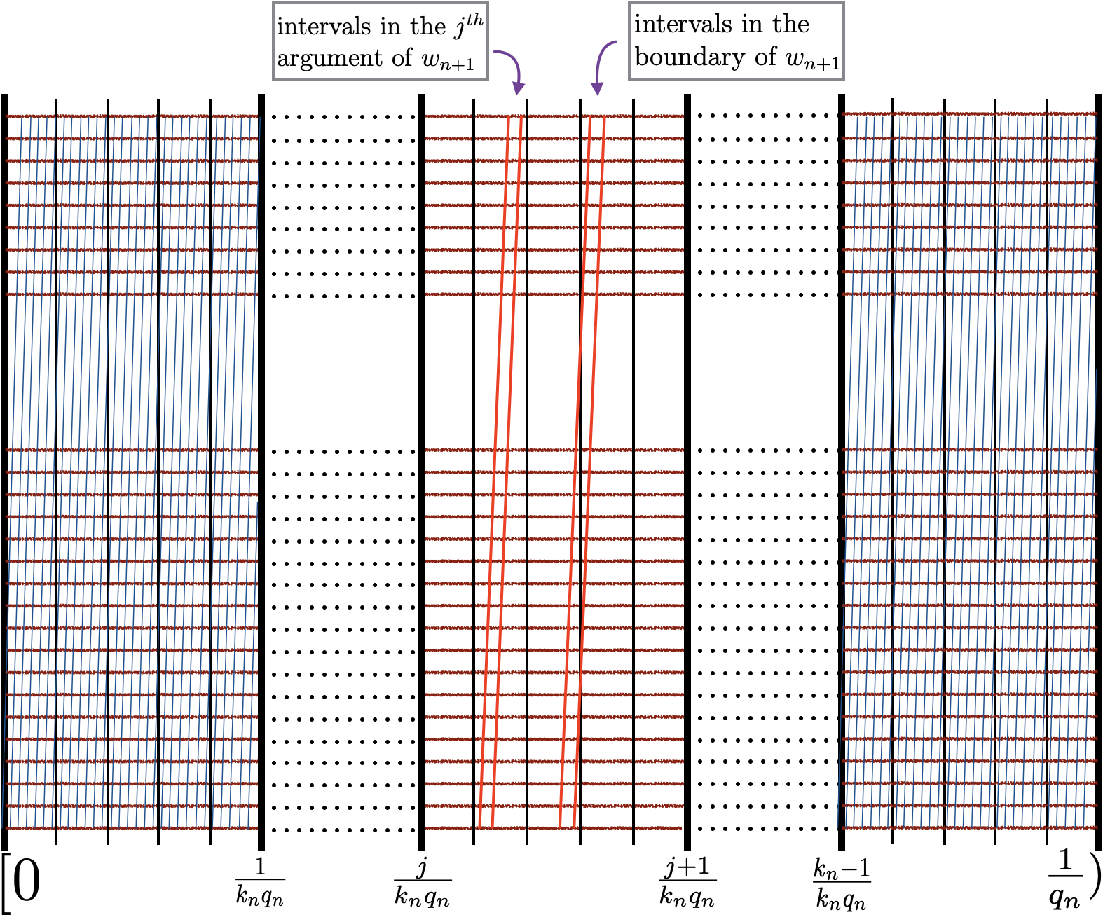
Figure 3: The $n$-tower, showing the diagonal progression of the $n+1$-tower. The heavy horizontal lines are the levels $(i\alpha_{n},i\alpha_{n}+1/q_{n})$, starting with $[0,1/q_{n})$ on the bottom. The levels the $n+1$-tower are the horizontal segments between the diagonal lines.

Again, following [13], the geometric picture in Figure 3 corresponds to the symbolic representation as a circular system in the following way. Some of the diagonal paths hit the left or right vertical strips bounding the $[j/k_{n}q_{n},(j+1)/k_{n}q_{n})$ subdivisions of the levels. Those diagonals correspond to the boundary portion of the $n+1$-words (the $b$’s and the $e$’s). The diagonal paths that start in the region $[j/k_{n}q_{n},(j+1)/k_{n}q_{n})$ and traverse from the bottom to the top level while staying in that region correspond to the $j^{th}$ argument of the ${\mathcal{C}}$ operator at stage $n$.

Restating this in terms of the isomorphism $\varphi_{0}$ between ${\mathcal{K}}_{\alpha}$ and $([0,1),\mathcal{R}_{\alpha})$, if $s_{1}$ and $s_{2}$ are mature elements of ${\mathcal{K}}_{\alpha}$ corresponding to $x_{1},x_{2}\in S^{1}$, then:

• $x_{1},x_{2}$ belong to two diagonal strips that do not touch a vertical strip and with base in the same interval $[j/k_{n}q_{n},(j+1)/k_{n}q_{n})$

  iff

• Inside their principal $n+1$-subwords, $s_{1}(0)$ and $s_{2}(0)$ are in $n$-words coming from the same argument $w^{\alpha}_{j}$ of ${\mathcal{C}}(w^{\alpha}_{0},w^{\alpha}_{1},\dots w^{\alpha}_{k_{n}-1})$.

We now continue the enumeration of basic notions in [11] we use here.

1. In a very slight variation of the notation of [11], when we are comparing $s$ with $t$ we define $d^{n}(s,t)=r_{n}(t)-r_{n}(s)$ (mod $q_{n}$). In this argument frequently $t={\mathcal{S}}_{\beta}(s)$ and if $\beta$ is clear from the context we simply write $d^{n}(s)$. If $x$ and $y$ correspond to $s$ and $t$, the number $d^{n}(s,t)$ can be viewed either as the number of levels in the $n$-tower between $x$ and $y$ or as the difference between the locations of $0$ in the principal $n$-subwords of $s$ and $t$.

2. For mature $s$ and $t$, the result of shifting $t$ by $-d^{n}(s,t)$ units is that the location of $0$ is in the same position in its principal $n$-subword as is the position of $s(0)$ in its principal $n$-subword.

3. Applying the shift map $d^{n+1}(s,t)$ times to $s$ moves its zero to the same point as $t$’s is relative to its $n+1$ subword. Subsequently moving it back $-d^{n}(s,t)$ steps moves the zero of result back to the same position in its $n$-subword as zero is in $s$’s $n$-subword. In other words, if $s^{\prime}$ is the result of applying the shift map to $s$ $d^{n+1}(s,t)-d^{n}(s,t)$ times, then $0$ is in the same position relative to the $n$-block of $s^{\prime}$ as it is in $s$.

4. The $n+1$-word in the construction sequence for ${\mathcal{K}}_{\alpha}$ is of the form

   $${\mathcal{C}}(w^{\alpha}_{0},w^{\alpha}_{1}\dots w^{\alpha}_{k_{n}-1})$$

   and hence if $s$ is mature at stage $n$ then $s(0)$ occurs in an $n$-block corresponding to the position of $w^{\alpha}_{j_{0}}$ for some $j_{0}$. We can ask whether the $j_{0}$ corresponding to the principal $n$-subword of the $(d^{n+1}(s,t)-d^{n}(s,t))$-shift of $s$ is the same as the $j_{0}$ corresponding to the principal $n$-subword of $s$.

   If it does, then $s$ and $t$ are well-matched at stage $n$ and if not the $s$ and $t$ are ill-matched at stage $n$.

5. If $s^{\prime}$ is the result of shifting $s$ $d^{n+1}(s,t)-d^{n}(s,t)$ times then the $0$ of $s^{\prime}$ is in the same $w^{\alpha}_{j}$ as is the zero of $t$. So for the purposes of determining whether $s$ is well-$\beta$-matched at stage $n$, we can compare which argument of ${\mathcal{C}}$ $s(0)$ and $t(0)$ belong to. As a result we can speak of $s$ and $t$ well or ill-matched at stage $n$. If $x$ and $y$ are the corresponding members of $[0,1)$ we can say say that $x$ and $y$ are well or ill-matched at stage $n$.

We are now ready to construct the non-central $\beta$. We do this by induction. At stage 1, $a_{1}=0$. At stage $n$, we let $\beta_{n}=\sum_{p=1}^{n-1}{a_{p}\over k_{p}q_{p}}$. For $i=0,\dots 6^{n}-1$, in the terminology of item 11 consider

$$M_{i}=\{x:x\mbox{ and }x+\beta_{n}+i/k_{n}q_{n}\mbox{ are well-matched}\}.$$

Since the $M_{i}$’s are disjoint, for some $i$, $\lambda(M_{i})\leq{1\over 6^{n}}$. Let $a_{n}$ be such an $i$ and let $\beta_{n+1}=\beta_{n}+a_{n}/k_{n}q_{n}$. Finally we let $\beta=\sum_{1}^{\infty}{a_{p}\over k_{p}q_{p}}$, so $\beta=\lim_{n\to\infty}\beta_{n}$.

To see this works, we first show that:

For almost all $x$, for large enough $m$, if $s_{m}$ corresponds to $x+\beta_{m}$ then for all mature $n\leq m,r_{n}(s_{m})=r_{n}({\mathcal{S}}_{\beta}(s))$.

This is a Borel-Cantelli argument. Note that if $r_{m}(s_{m})=r_{m}({\mathcal{S}}_{\beta}(s))$ then for all mature $n\leq m,r_{n}(s_{m})=r_{n}({\mathcal{S}}_{\beta}(s))$. Hence it suffices to show that for almost all $s$, all sufficiently large $m$, $r_{m}(s_{m})=r_{m}({\mathcal{S}}_{\beta}(s))$.

If $x$ corresponds to $s$ then the only way that $r_{m}(s_{m})\neq r_{m}({\mathcal{S}}_{\beta}(s))$ is if $x+\beta_{m}$ is in a different level of the $m$-tower than $x+\beta_{m}+\sum_{p=m}^{\infty}{a_{p}\over k_{p}q_{p}}$. In turn, the only way that this can happen is if for some $i$,

$$x+\beta_{m}\in[i\alpha_{m}+1/q_{m}-{\sum_{p=m}^{\infty}{a_{p}\over k_{p}q_{p}}},i\alpha_{m}+1/q_{m}).$$

The latter interval is the right hand portion of a level in the $m$-tower, i.e. of an interval of the form $[i\alpha_{m},i\alpha_{m}+1/q_{m})$.

The collection of $x$ that have this property for a given level $i$ has measure $\sum_{p=m}^{\infty}{a_{p}\over k_{p}q_{p}}$. Since there are $q_{m}$ many levels $i$, the measure of all of the $x$ with this property at stage $m$ is $q_{m}*\left(\sum_{p=m}^{\infty}{a_{p}\over k_{p}q_{p}}\right)$. Computing:

$$q_{m}*\left(\sum_{p=m}^{\infty}{a_{p}\over k_{p}q_{p}}\right) ={a_{m}\over k_{m}}+q_{m}*\sum_{m+1}^{\infty}{a_{p}\over k_{p}q_{p}}$$

$$<{a_{m}\over k_{m}}+{q_{m}\over q_{m+1}}\sum_{m+1}^{\infty}{a_{p}\over k_{p}}$$

$$\leq{a_{m}\over k_{m}}+{1\over k_{m}l_{m}q_{m}}C,$$

where $C=\sum_{1}^{\infty}{a_{p}\over k_{p}}$. Since we assume that $\sum{6^{n}\over k_{n}}<\infty$ and $a_{p}<6^{n-1}$, $C$ is finite. We see immediately that the measures of the collections of $x$ such that at some stage $m$ the level of $x+\beta_{m}$ in the $m$-tower is different from the level of $x+\beta$ in the $m$-tower is summable. By Borel-Cantelli, it follows that for almost all $s$ there is an $N$ for all $m\geq N$, $r_{m}(s_{m})=r_{m}({\mathcal{S}}_{\beta}(s))$.

From the choice of $a_{n}$ for all but a set of measure at most $1/6^{n}$, the $s$ are ill-matched with $s_{n+1}$. Again by the Borel-Cantelli lemma, for almost all $s$ there is an $N_{1}$ for all $n\geq N_{1}$ $s$ and $s_{n+1}$ are ill-matched. Since for almost all $s$ and all large enough $n$ the level of $s_{n+1}$ is equal to the level ${\mathcal{S}}_{\beta}(s)$ it follows that for almost all $s$ and all large enough $n$ $s$ is ill-matched with ${\mathcal{S}}_{\beta}(s)$. If $\nu$ is the unique invariant measure on ${\mathcal{K}}_{\alpha}$ then equation 33 of [11] defines

$$\Delta_{n}(\beta)=\nu(\{s:s\mbox{ is ill-$\beta$-matched at stage $n$}\}).$$

We have shown that $\Delta_{n}(\beta)\to_{n}1$. Hence

$$\Delta(\beta)=\sum_{n}\Delta_{n}(\beta)$$

is infinite. Hence we have shown that $\beta$ is not central. $\dashv$

We now prove Lemma 37

$\vdash$   ​​​ [Lemma 37] First note that the analysis in section 6.3, on page 50 of [11], says that for any non-central $\beta$ we can choose $hd_{1}$ and $hd_{2}$ and a spaced out set $G$ such that, as in equation 35 on page 50, letting

$$\not\Downarrow_{n}=\{s:s\mbox{ is ill-$\beta$-matched at stage $n$ and in configuration {$P_{{{hd_{1}},{hd_{2}}}}$}}\}$$

we get equation 36 on page 50 of [11]:

$$\sum_{n\in G}\nu(\not\Downarrow_{n})=\infty.$$ (18)

We now observe that for $n<m\in G$, $\not\Downarrow_{n}$ and $\not\Downarrow_{m}$ are probabilistically independent. This follows from Lemma 75 on page 47 of [11]: belonging to $\not\Downarrow_{n}$ is an issue of the value of $d^{n+1}-d^{n}$. The differences $d^{m+1}-d^{m}$ are independent of the differences $d^{n+1}-d^{n}$, hence the sets $\not\Downarrow_{n}$ and $\not\Downarrow_{m}$ are pairwise independent. Which level $x$ is on in the $n$-tower is independent of whether or not $x$ is misaligned at the next stage.

Let $M_{m}$ be the collection of $s$ that are mature at stage $m$. Then applying the “hard” Borel-Cantelli lemma, for almost all $s\in M_{m}$, there are infinitely many $n\in G,s\in\not\Downarrow_{n}$. Since $\bigcup_{m}M_{m}$ has measure one, for almost all $s\in{\mathbb{K}}^{c}$ there are infinitely many $n,s\in\not\Downarrow_{n}$.

We now argue that if $\mathcal{J}_{1}$ and $\mathcal{J}_{2}$ are two joinings of ${\mathbb{K}}^{c}\times{\mathbb{K}}^{c}$ over ${\mathcal{S}}_{\beta}$, then they are identical. Thus they are both the relatively independent joining. The result follows from the following claim which is an analogue of the claim in Proposition 32 of [9]:

Claim

Let $\mathcal{J}$ be a joining of ${\mathbb{K}}^{c}$ with itself that projects to the graph joining of ${\mathcal{K}}_{\alpha}$ with itself given by ${\mathcal{S}}_{\beta}$. Then for all cylinder sets $\langle a\rangle\times\langle b\rangle$ in ${\mathbb{K}}^{c}\times{\mathbb{K}}^{c}$, the density of occurrences of $(a,b)$ in a generic pair $(x,y)$ for $\mathcal{J}$ does not depend on the choice of $(x,y)$.

$\vdash$   Since $\beta$ is non-central, and $x,y$ are generic and $\mathcal{J}$ extends ${\mathcal{S}}_{\beta}$, we know that for infinitely many $n\in G$ the $n$-words of $x$ and $y$ are misaligned. Let $G^{*}$ be this set.

It suffices to show that:

• There is a sequence of subblocks of the principal $n+1$-subwords of $x$ and $y$ of total length $B_{n}$,

• as $n\in G^{*}$ goes to infinity, $B_{n}/q_{n+1}$ goes to $0$,

• after removing the subwords in $B_{n}$ the number of occurrences of $\langle a\rangle\times\langle b\rangle$ is independent of the choice of $(x,y)$.

Fix a large $n\in G^{*}$. We count occurrences of $(a,b)$ in $(x,y)$ over the portion of the principal $n+1$-subwords of $x$ that overlap with the $n+1$-blocks of $y$. As in Proposition 32 of [9], we show that, up to a negligible portion, this is independent of $(x,y)$. From the definition of $\not\Downarrow_{n}$ for $n\in G$, there are fixed values of $hd_{1}$ and $hd_{2}$. The number $hd_{2}$ determines the overlap of the $n+1$-block of $x$ containing $x(0)$ is the left or right overlap. For convenience, assume that $hd_{1}=L$ and $hd_{2}=R$.

First: discard $n$-subwords that are not mature. This is a negligible portion.

Next, shift $y$ back by $d^{n}(x)$, so that the mature $n$-subwords of $x$ in the principal $n+1$-subword are aligned along the overlap of the principal $n+1$ subword of $y$ with the corresponding $n$-subword of $y$.

Then by specification J.10.1 and the fact that $x$ and $y$ are misaligned, any pair of $n$–words $(u,v)$ occurs almost exactly $1/s_{n}^{2}$ times. So, after discarding a negligible portion of the occurrences all pairs occur the same number of times. Shifting them all back by $d^{n}(x)$, an amount determined by $\beta$ and thus independent of $x$ and $y$, gives a collection of counts of occurrences of $(a,b)$ in all pairs $(u,sh^{d^{n}}(v))$ with all pairs occurring essentially the same number of times. The result is independent of the choice of $x$ and $y$. The errors from the negligible portions and they go to zero in proportion to $n+1$. This proves the claim. $\dashv$

3.3 Diffeomorphisms of the Torus

The map $\mathcal{F}\circ F_{\mathcal{O}}$ maps codes for $\Pi^{0}_{1}$ sentences to construction sequence for circular systems. We now indicate how to realize circular systems as diffeomorphisms and why these diffeomorphisms are computable. The realization map is described completely in [13]. We review it here to verify its effectiveness.

The construction is in two stages. In both parts a sequence of periodic transformations is constructed and the limits are isomorphic to the given uniform circular system. In both constructions, the torus, viewed as $[0,1]\times[0,1]$ with appropriate edges identified, is divided into rectangles. These are then permuted by the periodic transformations according to the action of the shift operator on the circular system. In the first stage, this permutation is built without regard to continuity. The result is an abstract measure preserving transformation. In the second part, using smooth approximations to these permutations, the limit is a $C^{\infty}$ diffeomorphism.

The main tool for moving from the discontinuous, symbolic transformations to the smooth geometric transformations is the Anosov-Katok method of Approximation by Conjugacy [1]. To allow for this smoothing the parameter sequence $\langle k_{n},l_{n}:n\in\mathbb{N}\rangle$ must have the sequence of $l_{n}$’s grow sufficiently fast.

The lower bounds $l_{n}^{*}(\langle k_{m}:m\leq n\rangle,\langle l_{m}:m<n\rangle)$ will be determined inductively, the complete list of requirements on $l_{n}^{*}$ appears in Appendix A.

For the moment we assume we are given the circular sequence $\langle\mathcal{W}_{n}^{c}:n\in\mathbb{N}\rangle$ with prescribed coefficient sequences $\langle k_{n},l_{n}:n\in\mathbb{N}\rangle$ where the $l_{n}$ grow sufficiently fast.

The periodic approximations to the first stage transformation are of the form

$$T_{n}=Z_{n}\circ\operatorname{\overline{\mathcal{R}}}_{\alpha_{n}}\circ Z_{n}^{-1}$$ (19)

which result from conjugating horizontal rotations $(x,y)\mapsto_{\operatorname{\overline{\mathcal{R}}}_{\alpha_{n}}}(x+\alpha_{n},y)$, with the more complicated transformations $h_{n}:\mathbb{T}^{2}\to\mathbb{T}^{2}$ that permute rectangular subsets of $\mathbb{T}^{2}$. The $\alpha_{n}$ are the rationals constructed from the coefficient sequence $\langle k_{n},l_{n}:n\in\mathbb{N}\rangle$ described in section 3.1.1. The maps $Z_{n}$ are of the form

$$Z_{n}=h_{1}\circ h_{2}\circ\ldots\circ h_{n}$$

where $h_{i}$ codes the combinatorial behavior of the $i^{th}$ application of the ${\mathcal{C}}$-operation. The initial, discontinuous transformation $T$ will then be the almost-everywhere pointwise limit of the sequence $\langle T_{n}:n\in\mathbb{N}\rangle$.

In the second part of the construction the $h_{n}$’s will be replaced by smooth transformations $h_{n}^{s}$ that are close measure theoretic approximations to the $h_{n}$’s. This results in a new sequence

$$H_{n}=h_{1}^{s}\circ h_{2}^{s}\circ\dots\circ h_{n}^{s}.$$ (20)

The analogue of equation 19 for the final smooth transformation is:

$$S_{n}=H_{n}\operatorname{\overline{\mathcal{R}}}_{\alpha_{n}}H_{n}^{-1}$$ (21)

The sequence of $S_{n}$’s converge in the $C^{\infty}$-topology to a $C^{\infty}$ measure preserving transformation $S:\mathbb{T}^{2}\to\mathbb{T}^{2}$.

Why do we do this?

In [13] it is shown that $T$ is measure isomorphic to ${\mathbb{K}}^{c}$. Hence if ${\mathbb{K}}^{c}=\mathcal{F}\circ F(N)$ we have $\varphi_{N}$ is true if and only $T\cong T^{-1}$. Since $S\cong T$, $\varphi_{N}$ is true if and only $S\cong S^{-1}$. Thus if we define the realization function $R$ by setting $R({\mathbb{K}}^{c})=S$, we see that $R\circ\mathcal{F}\circ F_{\mathcal{O}}$ is a reduction of the collection of codes for true $\Pi^{0}_{1}$-sentences to the set of recursive diffeomorphisms isomorphic to their inverses. This is the content of figure 1.

In addition to these results in [13], we will show that the sequence of $S_{n}$’s can be taken to be effective, converge in the $C^{\infty}$ topology and that if $S(N)$ comes from $N$ and $S(M)$ comes from $M$, then $S(N)\not\cong S(M)$. This will complete the proof of Theorem 1.

3.3.1 Painting the circular system on the torus

We encode the symbolic system ${\mathbb{K}}^{c}$ on the torus by inductively constructing the sequence of $h_{n}$’s. The map $h_{0}$ is the identity map corresponding to $\mathcal{W}^{c}_{0}=\Sigma$. To build $h_{n+1}$, $\mathbb{T}^{2}$ is subdivided into rectangles which are then permuted.

Definition 38 (Rectangular subdivisions).

Let $n,m\in\mathbb{N}$.

• For an arbitrary natural number $q$, $\mathcal{I}_{q}$ represent the collection of intervals
  $[0,\tfrac{1}{q}),\ [\tfrac{1}{q},\tfrac{2}{q}),\ \ldots,[\tfrac{q-1}{q},1)$.

• Given $\mathcal{I}_{q}$ and $\mathcal{I}_{s}$, let $\mathcal{I}_{q}\otimes\mathcal{I}_{s}$ be the collection of all rectangles $R=I_{0}\times I_{1}$, where $I_{0}\in\mathcal{I}_{q}$ and $I_{1}\in\mathcal{I}_{s}$.

• Let $D\subseteq\mathbb{T}^{2}$. Then, for a collection of rectangles $\xi$, the restriction of $\xi$ to $D$ is given by

  $$\xi\mathbin{\upharpoonright}D=\{R\cap D:R\in\xi\}.$$

• Recall the parameter sequences $\langle q_{n}:n\in\mathbb{N}\rangle$ and $\langle s_{n}:n\in\mathbb{N}\rangle$. Further recall that $s_{n}=|\mathcal{W}^{c}_{n}|$ and $q_{n}=|u|$ for $u\in\mathcal{W}^{c}_{n}$. Define

  $$\xi_{n}=\mathcal{I}_{q_{n}}\otimes\mathcal{I}_{s_{n}}.$$

• Lastly, for $0\leq i<q_{n}$ and $0\leq j<s_{n}$, let $R^{n}_{i,j}$ be the element of $\xi_{n}$ given by $[\tfrac{i}{q_{n}},\tfrac{i+1}{q_{n}})\times[\tfrac{j}{s_{n}},\tfrac{j+1}{s_{n}})$.

Note that there is a straightforward description of the action of $\operatorname{\overline{\mathcal{R}}}_{\alpha_{n}}$ on $\xi_{n}$:

$$\operatorname{\overline{\mathcal{R}}}_{\alpha_{n}}:R^{n}_{i,j}\mapsto R^{n}_{i+p_{n},j}$$

where addition in the subscript is performed modulo $q_{n}$.

The map $h_{n+1}$ will be defined as a permutation of $\mathcal{I}_{k_{n}q_{n}}\otimes\mathcal{I}_{s_{n+1}}$ and thus induces a permutation of $\xi_{n+1}$. It is important to make $h_{n+1}$ commute with ${\overline{\mathcal{R}}}_{\alpha_{n}}$. To do this $h_{n+1}$ is first defined on $(\mathcal{I}_{k_{n}q_{n}}\otimes\mathcal{I}_{s_{n+1}})\mathbin{\upharpoonright}([0,1/q_{n})\times[0,1))$ and then copied over equivariantly to $\mathbb{T}^{2}$.

Constructing the $h_{n}$’s:

The paper [13] is concerned with realizing circular systems, and so builds the $h_{n}$’s in terms of the prewords used to construct the sequence $\langle\mathcal{W}_{n}^{c}:n\in\mathbb{N}\rangle$. In the case that $\langle\mathcal{W}_{n}^{c}:n\in\mathbb{N}\rangle$ is in the range of $\mathcal{F}$, the prewords are determined by the underlying odometer based sequence $\langle\mathcal{W}_{n}:n\in\mathbb{N}\rangle$. We describe $h_{n+1}$ directly in terms of the odometer sequence $\langle\mathcal{W}_{n}:n\in\mathbb{N}\rangle=F_{\mathcal{O}}(N)$.

Fix enumerations $\langle w^{n}_{s}:0\leq s<s_{n}\rangle$ of each $\mathcal{W}_{n}$. The words in $\mathcal{W}_{n+1}$ are concatenations of words in $\mathcal{W}_{n}$:

$$w^{n+1}_{s}=w_{0}w_{1}\dots w_{k_{n}-1}$$

where each $w_{i}=w^{n}_{s^{\prime}}$ for some $s^{\prime}$.

To each $w^{n+1}_{s}$ associate the horizontal strip $[0,1)\times[s/s_{n+1},(s+1)/s_{n+1})$ and each $w^{n}_{s^{\prime}}$ with $[0,1)\times[s^{\prime}/s_{n},(s^{\prime}+1)/s_{n})$.

Proposition 39.

There is a permutation of $\mathcal{I}_{k_{n}q_{n}}\otimes\mathcal{I}_{s_{n+1}}\mathbin{\upharpoonright}[0,1/q_{n})\times[0,1)$ such that for all $0\leq s<s_{n+1}$,

if $w_{i}=w^{n}_{s^{\prime}}$ then

$$h_{n+1}([i/k_{n}q_{n},(i+1)/k_{n}q_{n})\times[s/s_{n+1},(s+1)/s_{n+1}))$$ (22)

$$\subseteq[0,1/q_{n})\times[s^{\prime}/s_{n},(s^{\prime}+1)/s_{n}).$$

$\vdash$   Equation 22 gives regions that each atom of $\mathcal{I}_{k_{n}q_{n}}\otimes\mathcal{I}_{s_{n+1}}\mathbin{\upharpoonright}[0,1/q_{n})\times[0,1)$ must be sent to by $h_{n+1}$. To prove there is such a permutation we see that each region has exactly the same number of subrectangles as the cardinality of the collection of atoms that must map into it.

We count occurrences of $n$-words in $(n+1)$-words. Fix a word

$$w^{n+1}_{s}=w_{0}w_{1}\ldots w_{k_{n}-1}\in\mathcal{W}_{n+1}.$$

Then, by strong uniformity each $n$-word $w^{n}_{s^{\prime}}$ occurs $k_{n}/s_{n}$ times as a $w_{i}$. So each word $w^{n+1}_{s}$ puts $k_{n}/s_{n}$ rectangles in a target region. Since there are $s_{n+1}$ many words of the form $w^{n+1}_{s}$ the target regions must contain $s_{n+1}(k_{n}/s_{n})$ rectangles.

Each horizontal strip of $[0,1)\otimes\mathcal{I}_{s_{n}}$ is divided into $s_{n+1}/s_{n}$ many horizontal strips by $[0,1)\otimes\mathcal{I}_{s_{n+1}}$ and each vertical strip of $\mathcal{I}_{q_{n}}\otimes[0,1)$ is divided into $k_{n}$ many vertical strips by $\mathcal{I}_{k_{n}q_{n}}\otimes[0,1)$. Thus each atom of the partition $\xi_{n}\mathbin{\upharpoonright}[0,1/q_{n})\times\mathcal{I}_{s}$ is divided into $k_{n}(s_{n+1}/s_{n})$ rectangles by $\mathcal{I}_{k_{n}q_{n}}\otimes\mathcal{I}_{s_{n+1}}$. In particular $\mathcal{I}_{k_{n}q_{n}}\otimes\mathcal{I}_{s_{n+1}}\mathbin{\upharpoonright}[0,1/q_{n})\times[s^{\prime}/s_{n},(s^{\prime}+1)/s_{n})$ has $k_{n}(s_{n+1}/s_{n})$ many atoms.

Hence each target region contains the same number of rectangles as atoms sent to it and there is a map $h_{n+1}$ satisfying equation 22. $\dashv$

Since $h_{n+1}$ is a permutation of $\mathcal{I}_{k_{n}q_{n}}\otimes\mathcal{I}_{s_{n+1}}\mathbin{\upharpoonright}[0,1/q_{n})\times[0,1)$ for each $1\leq i<q_{n}$, it can be copied onto each $\mathcal{I}_{k_{n}q_{n}}\otimes\mathcal{I}_{s_{n+1}}\mathbin{\upharpoonright}[ip/q_{n},(ip+1)/q_{n})$. The result of this is a permutation of $\mathcal{I}_{k_{n}q_{n}}\otimes\mathcal{I}_{s_{n+1}}$ (and hence $\xi_{n+1}$) that commutes with the rotation ${\overline{\mathcal{R}}}_{\alpha_{n}}$.

Remark 40.

It is a clear that $h_{n+1}$ can be defined in a primitive recursive way using the data $\mathcal{W}_{n+1}$.

Remark

It is shown in [13] that having defined the sequence of $h_{n}$’s in this manner, for sufficiently fast growing $l_{n}$ the transformations $T_{n}$ converge in measure to a measure preserving transformation $T:(\mathbb{T}^{2},\lambda)\to(\mathbb{T}^{2},\lambda)$ that is isomorphic to the original circular system defined by $\langle\mathcal{W}_{n}^{c}:n\in\mathbb{N}\rangle$. The map taking $\langle\mathcal{W}^{c}_{m}:m\leq n\rangle$ to $T_{n}$ is primitive recursive.

3.3.2 Smoothing the $T_{n}$

We now must smooth the $T_{n}$’s to produce $S_{n}$’s that have measure-theoretic limit $S$ which is isomorphic to $T$. Secondly, we show that $S$ is a recursive diffeomorphism.

For our discussion of smoothing we need an effective complete metric on the $C^{\infty}$-diffeomorphisms. Note that the $C^{\infty}$ topology is the coarsest common refinement of the $C^{k}$ topologies for each $k\in\mathbb{N}$. There are many choices for effective/recursive metrics generating the $C^{k}$ topology for each $k$; for instance the metric derived from the norm given by

$$\|f\|_{k}=\max_{x\in\mathbb{T}^{2}}\|f(x)\|^{0}+\|Df(x)\|^{1}+\cdots+\|D^{k}f(x)\|^{k}$$

where $\|-\|^{j}$ is the $j$-norm on $\mathbb{R}^{2j+2}$. Given an effective sequence of complete metrics $\langle d^{k}:k\in\mathbb{N}\rangle$ generating the $C^{k}$ topologies, with distances bounded by 1, then

$$d^{\infty}=\sum_{k=0}^{\infty}2^{-(k+1)}d^{k}$$

generates the $C^{\infty}$ topology.

Fix such a complete effective metric giving rise to the $C^{\infty}$ topology on $\mathbb{T}^{2}$. Without loss of generality we can assume that

$$d^{\infty}(S,T)\leq\max_{x\in\mathbb{T}^{2}}d_{\mathbb{T}^{2}}(S(x),T(x)),$$ (23)

where $d_{\mathbb{T}^{2}}$ is the ordinary metric on $\mathbb{T}^{2}$.

To pass from the discontinuous $Z_{n}$’s to diffeomorphisms, the $h_{i}$’s are replaced by smooth $h^{s}_{i}$ which are very close approximations and give the $H_{n}$’s in equation 20. Then the $H_{n}$’s will also be diffeomorphisms. While there is no control over the $C^{\infty}$-norms of the $H_{n}$, the key observation at the heart of the Anosov-Katok method is the following: if $h^{s}_{n+1}$ commutes with $\operatorname{\overline{\mathcal{R}}}_{\alpha_{n}}$ then

$$S_{n} =H_{n}\circ\operatorname{\overline{\mathcal{R}}}_{\alpha_{n}}\circ H_{n}^{-1}$$

$$=H_{n}\circ h^{s}_{n+1}\circ(h^{s}_{n+1})^{-1}\circ\operatorname{\overline{\mathcal{R}}}_{\alpha_{n}}\circ H_{n}^{-1}$$

$$=H_{n}\circ h^{s}_{n+1}\circ\operatorname{\overline{\mathcal{R}}}_{\alpha_{n}}\circ(h^{s}_{n+1})^{-1}\circ H_{n}^{-1}$$

$$=H_{n+1}\circ\operatorname{\overline{\mathcal{R}}}_{\alpha_{n}}\circ H_{n+1}^{-1}.$$ (24)

Hence by taking $\alpha_{n+1}$ sufficiently close to $\alpha_{n}$, $S_{n+1}$ can be taken as close as necessary to $S_{n}$ in the $C^{\infty}$-norm.

To carry out this plan we begin by describing how we smooth the $h_{n}$’s. This is done explicitly in Theorem 35 of [13], which says:

Theorem 41 (Smooth permutations).

Let $\mathbb{T}^{2}$ be divided into the collection of rectangles $\mathcal{I}_{n}\otimes\mathcal{I}_{m}$ and choose $\epsilon>0$. Let $\sigma$ be a permutation of the rectangles. Then there is an area preserving $C^{\infty}$-diffeomorphism $\varphi:\mathbb{T}^{2}\to\mathbb{T}^{2}$ such that $\varphi$ is the identity on a neighborhood of the boundary of $[0,1]\times[0,1]$ and for all but a set of measure at most $\epsilon$, if $x\in R$, then $\varphi(x)\in\sigma(R)$ for all $R\in\mathcal{I}_{n}\otimes\mathcal{I}_{m}$.

In Lemma 36 of [13] it is shown that an arbitrary permutation of $\mathcal{I}_{n}\otimes\mathcal{I}_{m}$ can be built by taking a composition of transpositions of adjacent rectangles. The transformation $\varphi$ is then built effectively as a composition of smooth near-transpositions that swap adjacent rectangles. We summarize the proof. More details appear in Appendix D, where it is shown that it can be carried out recursively in a code for the permutation $\sigma$.

The main technical point for building the near-transpositions of adjacent rectangles is captured by showing that for all $0<\gamma<1$ and arbitrarily small $\epsilon<1-\gamma$, there is a diffeomorphism $\varphi_{0}$ of the unit disk in $\mathbb{R}^{2}$ such that:

1. $\varphi_{0}$ rotates the top half of the disk of radius $\gamma$ to the bottom half and vice versa.

2. $\varphi_{0}$ is the identity in a neighborhood of the unit circle of width less than $\epsilon$.

The map $\varphi_{0}$ is constructed by considering a primitive recursive $C^{\infty}$ map $f:[0,1]\to[0,\pi]$ that is identically equal to $\pi$ on $[0,\gamma]$ and is $0$ in a neighborhood of 1. Then $\varphi_{0}$ rotates the circle of radius $r$ by $f(r)$ radians. Taking $\gamma$ very close to $1$ gives a smooth near transposition.

Using Riemann mapping theorem techniques, these rotations of the disk can be copied over to measure preserving maps from $[-1,1]\times[0,1]$ to itself that

1. take all but $1-\epsilon/2$ mass of $[-1,0]\times[0,1]$ to $[0,1]\times[0,1]$ and vice versa,

2. are analytic on the interior of $[-1,1]\times[0,1]$,

3. are the identity in a neighborhood of the boundary.

Since every permutation of $\{0,1,\dots mn\}$ can be written as a composition of less than or equal to $(nm)^{2}$ transpositions of the form $(k,k+1)$, given any $\sigma$ we can build $\varphi$ by taking $\epsilon$ small enough and composing sufficiently good approximations between adjacent rectangles corresponding to the transpositions composed to create $\sigma$.

Building $S_{n}$.

Using Theorem 41 we can effectively choose a smooth $h^{s}_{n+1}$ which well-approximates $h_{n+1}$ measure theoretically. By choosing the approximation well, we can guarantee that the $S_{n}$ in equation 21 moves the partitions $\xi_{n}$ very close to where the $T_{n}$’s move the $\xi_{n}$’s.

Since $h^{s}_{n+1}$ is effective, using the continuity of composition with respect to $d^{\infty}$, $S_{n+1}$ can be made arbitrarily close to $S_{n}$ by taking $\alpha_{n+1}$ sufficiently close to $\alpha_{n}$. Thus if $\alpha_{n}$ converges to $\alpha$ sufficiently quickly, the sequence $\langle S_{n}:n\in\mathbb{N}\rangle$ is Cauchy with respect to the complete metric $d^{\infty}$ and hence converges to a smooth measure preserving diffeomorphism $S$. Taking the sequence of $h^{s}_{n}$’s to be sufficiently close to the $h_{n}$’s the $S_{n}$’s are sufficiently close to the $T_{n}$’s to apply Lemma 30 of [13] to show that the diffeomorphism $S$ is measure theoretically isomorphic to $T$. Hence $(\mathbb{T}^{2},\lambda,S)$ is measure theoretically isomorphic to $({\mathbb{K}}^{c},\nu,\operatorname{\textsc{Sh}})$.

The induction.

The discussion above was predicated on choosing the $l_{n}$’s to grow fast enough. We now show how to inductively choose lower bounds $l_{n}^{*}$ on the $l_{n}$. Numerical Requirement E gives one collection of lower bounds for the $l$’s, independently of the choices of the maps $H_{n}$ and numbers $\alpha_{n}$. Hence we choose $l_{n}^{*}$ to dominate this sequence of lower bounds, as well as the lower bounds we add here.

Suppose we have defined $H_{n+1}$ from $h_{n+1}^{s}$ and $H_{n}$ in a manner that satisfies equation 3.3.2 holds and that the $H_{n}$’s can be computed effectively. Then, for any given $\epsilon$, and small rational $\beta$,

$${d^{\infty}(H_{n+1}{\overline{\mathcal{R}}}_{\alpha_{n}+\beta}H^{-1}_{n+1},H_{n}{\overline{\mathcal{R}}}_{\alpha_{n}}H^{-1}_{n})}$$ (25)

can be primitively recursively computed to within a given $\epsilon$. Moreover, this is a decreasing function of $\beta$ for small $\beta>0$. Thus one one can effectively find a $\delta$ such that if $|\alpha_{n+1}-\alpha_{n}|<\delta$, then $d^{\infty}(S_{n+1},S_{n})<2^{-(n+1)}$.

Recall the definitions of the $\alpha_{n}=p_{n}/q_{n}$ from equations 13, 14 and 15. Then $\alpha_{n}$ does not depend on $l_{n}$ and

$$\alpha_{n+1}=\alpha_{n}+{1/k_{n}l_{n}q_{n}^{2}}.$$

Thus to make $\alpha_{n+1}$ close to $\alpha_{n}$ it suffices to make $l_{n}$ sufficiently large that

$$1/k_{n}l_{n}q_{n}^{2}<\delta.$$ (26)

Numerical Requirement G

The parameter $l_{n}$ is chosen sufficiently large that

$$d^{\infty}(S_{n+1},S_{n})<2^{-(n+1)}$$ (27)

The numbers $\alpha_{n}$, $\langle\mathcal{W}^{c}_{m}:m\leq n\rangle$ and $\langle h^{s}_{m}:m\leq n+1\rangle$ determine the $\delta$ in equation 26 and thus how large $l_{n}$ must be. All of this data can be computed recursively from $\langle\mathcal{W}_{m}:m\leq n+1\rangle$. (We note that neither the choice of $s_{n+1}$ nor the definition $h^{s}_{n+1}$ uses $l_{n}$.)

3.3.3 The effective computation of $S_{n}$

We now show that each element of the sequence $\langle S_{n}:n\in\mathbb{N}\rangle$ is effectively computable (Definition 7).

Claim 42.

The functions $h_{n}^{s}$ and $\mathcal{R}_{\alpha_{n}}$ are effectively computable $C^{\infty}$-functions. As a consequence each $S_{n}$ is effectively uniformly continuous.

Proof of Claim 42.

For simplicity of exposition, we only show how to compute the modulus of continuity and approximation for $S_{n}$ itself; finding the modulus of continuity and approximations to the higher differentials is conceptually identical but notationally cumbersome.

Recall that we must produce two functions:

• A modulus of continuity, $d:\mathbb{N}\to\mathbb{N}$, and

• An approximation, $f:(\{0,1\}\times\{0,1\})^{<\mathbb{N}}\to(\{0,1\}\times\{0,1\})^{<\mathbb{N}}$.

It is routine to check that if $T_{0}$ and $T_{1}$ are effectively uniformly continuous—that is, if there exist moduli of continuity $d_{0}$ and $d_{1}$ and approximations $f_{0}$ and $f_{1}$ corresponding to each—then the composition, $T_{1}\circ T_{0}$ is effectively uniformly continuous.

The second part of the claim follows from the first since Equations (21) and (20) show,

$$S_{n}=h_{1}^{s}\circ h_{2}^{s}\circ\cdots\circ h_{n}^{s}\circ\operatorname{\overline{\mathcal{R}}}_{\alpha_{n}}\circ(h_{n}^{s})^{-1}\circ\cdots\circ(h_{2}^{s})^{-1}\circ(h_{1}^{s})^{-1}.$$ (28)

The case of $\operatorname{\overline{\mathcal{R}}}_{\alpha_{n}}$ is particularly simple. Since $\operatorname{\overline{\mathcal{R}}}_{\alpha_{n}}$ is an isometry, it has a Lipschitz constant of $1$. In particular, the modulus of continuity is simply given by $d(n)=n$, and, since $\operatorname{\overline{\mathcal{R}}}_{\alpha_{n}}$ is well-defined on rational points, we can also determine the approximation by setting $f$ to be

$$([x]_{m},[y]_{m})\mapsto([x]_{m}+[\alpha_{n}]_{m},[y]_{m})$$

Where $[z]_{m}$ denotes the smallest dyadic rational $k\times 2^{1-m}$ for $0\leq k\leq 2^{m}$ minimizing $|z-[z]_{m}|$.

In the case of $h_{m}^{s}$ for $m\leq n$, recall from the discussion after Theorem 41 that $h^{s}_{m}$ can be built as a composition of a sequence of smooth transpositions:

$$h_{m}^{s}=\sigma_{0}^{s}\circ\sigma_{1}^{s}\circ\cdots\circ\sigma_{t(m)}^{s}$$

Note that the number of transpositions necessary, $t(m)<|\xi_{m+1}|^{2}=(k_{m}\cdot q_{m}\cdot s_{m+1})^{2}$, and is a computable function of $m$ since it is the number of transpositions necessary to build the permutation in Proposition 39.

Since $\sigma_{j}^{s}$ is a smooth transposition of an explicit form (given in Appendix D), one can calculate a uniform Lipschitz constant $L_{j}^{s}$ for it; hence, taking $L_{m}>\max_{s\leq t(m)}L^{s}_{j}$, we have that

$$|h_{m}^{s}(x)-h_{m}^{s}(y)|<(L_{m})^{t(m)+1}|x-y|.$$

Consequently, a suitable modulus of continuity for $h_{m}^{s}$ is given by

$$d(n)=n+\lceil t(m)\cdot\log_{2}(L_{m})\rceil,$$ (29)

where $\lceil x\rceil$ is the smallest integer greater than $x$. The construction of a primitive recursive approximation to $h_{m}^{s}$ is straightforward from the primitive recursive approximations to the $\sigma^{s}_{n}$’s. As we remarked in Section 1.4, it follows that $(h_{m}^{s})^{-1}$ is primitive recursive. $\dashv$

In summary, the modulus of continuity and approximation for $S_{n}$ can be calculated using the following steps:

1. Compute the $\langle h_{m}:m\leq n\rangle$;

2. Build the approximations to $h_{m}^{s}$ and $(h_{m}^{s})^{-1}$ using $h_{m}$ and the smooth transpositions given in Appendix D for $m\leq n$;

3. Compute the moduli of continuity of $\langle h^{s}_{m}:m\leq n\rangle$ and their inverses;

4. Compute $\langle\alpha_{m}:m\leq n\rangle$ (and, consequently, the approximations and moduli of continuity for $\langle\operatorname{\overline{\mathcal{R}}}_{\alpha_{m}}:m\leq n\rangle$);

5. Compute the approximation and modulus of continuity of $S_{n}$ by composing the approximations and moduli of continuity calculated in Steps 1 through 4 according to Equation (28).

3.4 Completing the proof

Theorem 1 claims the existence a computable function $F$, which on inputting a natural number $N$ (corresponding to the $\Pi^{0}_{1}$ sentence $\varphi$) outputs a code for a computable diffeomorphism $S(N)$ of $\mathbb{T}^{2}$. Whether or not $S(N)$ is measure theoretically conjugate to $S(N)^{-1}$ is equivalent to the truth of falsity of $\varphi$. Finally for different numerical inputs the corresponding $S$’s will not be isomorphic. In summary, letting $S=S(N)$,

1. If $N$ codes $\varphi$, then $\varphi$ is true if and only iff $S\cong S^{-1}$

2. On input $N$, $F$ recursively determines a code for an effectively $C^{\infty}$ map of the torus to itself, i.e., $F$ determines:

   1. A computable function $d:\mathbb{N}\times\mathbb{N}\to\mathbb{N}$, where $d(k,-)$ computes the moduli of uniformity of the $k^{th}$ differential of $S(N)$, and

   2. A computable function $f(k,-)$ where $f(k,-)$ is a map on dyadic rational points of $\mathbb{T}^{2}$ approximating $D^{k}S(N)$ (the $k$-th differential of $S(N)$). Given an input that is precise to $d(k,n)$ digits, $f(k,-)$ approximates the first $n$-partial derivatives $\{{\partial^{n}\over\partial^{i}x\partial^{n-i}y}:0\leq i\leq n\}$ to $n$-digits.

3. If $N\neq M$, then the associated diffeomorphisms $S(N)$ and $S(M)$ are not conjugate.

Because the function $F$ maps natural numbers to natural numbers (the codes for the diffeomorphisms) we let $F^{\flat}$ be the associated function $R\circ\mathcal{F}\circ F_{\mathcal{O}}$ that maps into the space of actual diffeomorphisms. It produces a diffeomorphism of $\mathbb{T}^{2}$ from a Gödel number $N$ for a $\Pi^{0}_{1}$ set. We show $F^{\flat}$ satisfies $(A)$ and $(C)$ and then argue there is a (primitively) computable routine coded by $F(N)$ that has the same values.

Item (A)

Given $N$, $F_{\mathcal{O}}(N)$ computes an odometer-based construction sequence $\langle\mathcal{W}_{n}:n\in\mathbb{N}\rangle$. By Theorem 9, if ${\mathbb{K}}(N)$ is the uniquely ergodic symbolic shift associated with the construction sequence then ${\mathbb{K}}(N)\cong{\mathbb{K}}(N)^{-1}$ if and only if $\varphi$ is true.

The sequences $\langle l_{n}:n\in\mathbb{N}\rangle$, $\langle\mathcal{W}_{n}^{c}:n\in\mathbb{N}\rangle$ and $\langle h_{n}^{s}:n\in\mathbb{N}\rangle$ are computed. If ${\mathbb{K}}^{c}$ is the circular system associated with $\langle\mathcal{W}_{n}^{c}:n\in\mathbb{N}\rangle$, then Proposition 35 shows that ${\mathbb{K}}^{c}\cong({\mathbb{K}}^{c})^{-1}$ if and only if $\varphi$ is true.

Finally the realization map $R$ preserves isomorphism. So if $S=R({\mathbb{K}}^{c})$, then $(\mathbb{T}^{2},\lambda,S)\cong(\mathbb{T}^{2},\lambda,S^{-1})$ if and only if $\varphi$ is true.

Item (C)

We need to see that for $M<N,S(N)\not\cong S(M)$. Since the realization map $R$ preserves isomorphism if suffices to see that $({\mathbb{K}}^{c})^{M}=\mathcal{F}\circ F_{\mathcal{O}}(M)$ is not isomorphic to $({\mathbb{K}}^{c})^{N}$.

By Corollary 34 we see that the Kronecker factor of ${\mathbb{K}}^{M}$ is ${\mathcal{K}}_{\alpha^{M}}$. Any isomorphism between $({\mathbb{K}}^{c})^{N}$ and $({\mathbb{K}}^{c})^{M}$ must take the respective Kronecker factor of one to the other, hence would imply an isomorphism between ${\mathcal{K}}_{\alpha^{N}}$ and ${\mathcal{K}}_{\alpha^{M}}$.

However this is impossible since Corollary 34 implies that $\pi>\alpha^{M}>\alpha^{N}>0$.

Item (B)

$F^{\flat}$ is a map from $\mathbb{N}$ to diffeomorphisms. By the result of Section 3.3.3, the diffeomorphisms are recursive. We must show that there is a recursive algorithm coding a function $F$ that computes the moduli of continuity and approximations to each $F^{\flat}(N)$ and its differentials.

We use the notation $\mathbbm{d}^{N}$ to denote the modulus of continuity returned by $F(N)$, and we use the notation $\mathbbm{f}^{N}$ to denote the approximation. Without loss of generality, we restrict our attention to $d(0,-)$ and $f(0,-)$—that is, the $C^{0}$ modulus of continuity and approximation of $S$. The calculation for $d(k,-)$ and $f(k,-)$ for $k>0$ is virtually identical conceptually. We simplify the notation of (B) above and write $\mathbbm{d}^{N}(n)$ for $d(0,n)$ and $\mathbbm{f}^{N}(\vec{s},\vec{t})$ for $f(0,\vec{s},\vec{t})$.

Let us first consider the modulus of continuity. The routine for computing $\mathbbm{d}^{N}$ depends on choosing a large number of numerical parameters:

$$\epsilon_{n},e(n),s_{n},k_{n},l_{n},P_{N}.$$

These have numerical dependencies that are generally of the form $a_{n}\gg b_{n}$ or $a_{n}\ll b_{n}$. It is routine that these can be satisfied in a primitive recursive manner–provided that the dependencies are consistent. This is verified in Appendix A where it is shown that the dependencies among these constants form a directed acyclic graph.

The subroutine we describe next comes during the computation of $F(N)$, and hence we may assume that we have the coefficients $k_{n}(N-1),l_{n}(N-1)$ already computed. This computation was made during the first $n$ steps of the computation of $F(N-1)$, but we neglect that recursion in this discussion.

For the inductive construction we note that:

For each $0\leq m\leq n+1$, make the following calculations, which recursively depend on smaller $m$. Specifically, $\mathcal{W}_{m}$ is built from $\mathcal{W}_{m-1}$ using the Substitution Lemma (Proposition 20) as described in section 2.6. Then $h_{m}^{s}$ is built from the information in the words in $\mathcal{W}_{m}$. This allows $l_{m}$ to be chosen large enough that Numerical Requirement G holds. This in turn defines $p_{m}$ and $q_{m}$ and allows $\mathcal{W}^{c}_{m}$ to be built.

The algorithm is illustrated in Figure 4.

1. Using $\langle\epsilon_{k}:k\leq m\rangle$ and $\mathcal{W}_{m-1}$, choose $k_{m}$ large enough to satisfy the Numerical Requirements C and D and apply the Substitution Lemma $m+1$ times to generate $\mathcal{W}_{m}$;

2. Build $h_{m}$, smooth it to get $h_{m}^{s}$ and hence $H_{m}$. Calculate $H_{m}$’s modulus of continuity.

3. Choose $l_{m}$ sufficiently large that Numerical Requirements E and F hold (with $n+1=m$).

4. Build $\mathcal{W}_{m}^{c}$.

5. Calculate the approximation and modulus of continuity corresponding to $S_{m}$ using the methods of Section 3.3.3.

6. Continue until $m=n+1$ and $d^{S_{N}}(n+1)$, the $n+1^{st}$ approximation to the modulus of continuity of $S_{n+1}$ is determined.

7. Output $d(n+1)(n+1)=d^{S_{N}}(n+1)$.

At the end, using the modulus of continuity $d$ corresponding to $S_{n+1}$, output $\mathbbm{d}^{N}(n)=d(0,n+1)$ where $d(n+1)$ is the modulus of continuity of $S_{n+1}$.

To verify that this procedure actually yields a modulus of continuity for $S$, recall that by Numerical Requirement G, Equation (27), it follows that

$$d^{\infty}(S_{n+1},S)<2^{-(n+1)}.$$

By inequality 23,

$$\max_{x\in\mathbb{T}^{2}}d_{\mathbb{T}^{2}}(S_{n+1}(x),S(x))\leq d^{\infty}(S_{n+1},S)<2^{-(n+1)}.$$

Since $d(n+1)$ yields the number of digits of input necessary to approximate $S_{n+1}$ to an accuracy of $2^{-(n+1)}$, it follows that the approximation of $S_{n+1}$ is itself an approximation of $S$ which, given $d(n+1)$ digits of binary input, is accurate to within $2^{-n}$.

Figure 4: The algorithm for calculating the modulus of continuity $d^{N}$ of $S$. This algorithm is easily altered to produce the approximation $\mathbbm{f}^{N}$ of $S$ simply by changing the output to $(f_{0}(\vec{x}),f_{1}(\vec{y}))$, where $f(n+1)=(f_{0},f_{1})$ is $S_{n+1}$’s approximation.

The approximation $f$ for $S$ is calculated almost identically, except for the output. Given

$$([x]_{\mathbbm{d}^{N}(n)},[y]_{\mathbbm{d}^{N}(n)})\in(\{0,1\}\times\{0,1\})^{d(n)}$$

the output is

$$\mathbbm{f}^{N}(n+1)=\left(f_{0}([x]_{\mathbbm{d}^{N}(n)}),f_{1}([y]_{\mathbbm{d}^{N}(n)})\right)$$

where $f(n+1)=(f_{0},f_{1})$ is the approximation of $S_{n+1}$ produced in Step 5, again in the notation that $[z]_{m}$ is a $m$-digit binary approximation of $z$.

Appendices

Appendices B-D were originally written by Johann Gaebler. The author has cleaned up exposition and done his best to fix various mistakes that appeared in Gaebler’s original version.

Appendix A Numerical Parameters

A.1 The Numerical Requirements Collected.

In this appendix we review the requirements on the numerical parameters used in the construction. Specifically, in constructing the diffeomorphism $F(N)$ we build construction sequences $\langle\mathcal{W}_{n}:n\in\mathbb{N}\rangle$, $\langle\mathcal{W}_{n}^{c}:n\in\mathbb{N}\rangle$ that depend on $N$ and realize the corresponding circular system ${\mathbb{K}}^{c}$ as a diffeomorphism. These steps are intertwined–for example the circular system is built as a function of the sequence $\langle k_{n},l_{n}:n\in\mathbb{N}\rangle$. In turn the $l_{n}$ are chosen as function of $\langle\mathcal{W}_{m}:m\leq n\rangle$ in order to facilitate the smooth construction. To rigorously complete the proof we need to review all of these parameters and see that the inductive choices can be made consistently in a primitive recursive way.

At many stages in this paper we appeal to results from [11]. Hidden in those appeals is a sequence of parameters $\langle\mu_{n}:n\in\mathbb{N}\rangle$ that is not explicitly mentioned in the construction presented here. For this reason this review includes the inductive construction of $\langle\mu_{n}:n\in\mathbb{N}\rangle$.

A substantial difference between this paper and earlier constructions is that the domain of the reductions in [9] and [11] is the space of trees of finite sequences of natural numbers. The analogue in this paper is that the only trees considered here are the trees of sequences $\langle(0,1,\dots n):n<\Omega\rangle$ for $\Omega$ finite or infinite depending on the input $N$. We note that these trees are really “stalks” and are finite or infinite depending on $\Omega$. Since the trees we consider in this paper are of this very special form, the requirements are easier to satisfy.

Closely following section 10 of [11] we begin with a review of the inductive requirements from [9]. We give them in the notation of [11]. These inductive requirements are modified and simplified in the construction in the current manuscript. We note the versions used in this paper.

Requirements that were instituted in [9] and their modifications.

These requirements were dubbed Inherited Requirements in [11]. Requirements that were new in [11] are called simply Numerical Requirements, and requirements that explicitly mentioned in the text of the paper are labelled with capital letters A-F.

Recall that the number of elements of $\mathcal{W}_{m}$ is denoted $s_{m}$; the numbers $Q^{m}_{s}$ and $C^{m}_{s}$ denote the number of classes and sizes of each class of $\mathcal{Q}^{m}_{s}$ respectively. From the construction in [9] we have sequences $\langle\epsilon_{n}:n\in\mathbb{N}\rangle$, $\langle s_{n},k_{n},e(n):n\in\mathbb{N}\rangle$.

Inherited Requirement 1

$\langle\epsilon_{n}:n\in\mathbb{N}\rangle$ is summable.

Inherited Requirement 2

$2^{e(n-1)}$ the number of $\mathcal{Q}^{n}_{i+1}$ classes inside each $\mathcal{Q}^{n}_{i}$ class. The numbers $e(n)$ will be chosen to grow fast enough that

$$2^{n}2^{-e(n)}<\epsilon_{n}$$ (30)

Similarly we set $C^{n}_{n}=2^{e(n)}$ as well.

Modification: In this paper the construction is simplified so to build $\mathcal{W}_{n+1}$ we have exactly $n+2$-substitutions of each of size $2^{2e(n)}$. Hence we can replace this requirement by the simple formula $s_{n}=2^{(n+1)e(n-1)}$. In particular $s_{m},Q^{m}_{i}$ and $C^{m}_{i}$ are all to be powers of 2.

Inherited Requirement 3

For all $n$,

$$2\epsilon_{n}s_{n}^{2}<\epsilon_{{n-1}}$$ (31)

Inherited Requirement 4

$$\epsilon_{n}k_{n}s_{{n-1}}^{-2}\to\infty\mbox{ as }n\to\infty$$ (32)

Inherited Requirement 5

$$\prod_{n\in\mathbb{N}}(1-\epsilon_{n})>0$$ (33)

Comment: Since this is equivalent to the summability of the $\epsilon_{n}$-sequence, it is redundant and we will ignore in the rest of this paper

Inherited Requirement 6

(Original Version) There will be prime numbers $p_{i}$ such that $K_{i}=p_{i}^{2}s_{i-1}K_{i-1}$ (i.e. $k_{i}=p_{i}^{2}s_{{i-1}}$). The $p_{n}$’s grow fast enough to allow the probabilistic arguments in [9] involving $k_{n}$ to go through.

Modification For all $n$, $k_{n}=P_{N}2^{\ell}s_{{n}}$, where for each $n$, $\ell$ is large enough for the substitution argument involving $k_{n}$ to go through.

Comment: In [9] $K_{n}$ was a product of a sequence of prime numbers. The requirement on the sequences of prime numbers was that they were almost disjoint for different trees and that they grew sufficiently quickly. In this paper $K_{N}$ is $P_{N}*2^{\ell}$ for a large $\ell$.

Since we have only one collection of very special trees the requirement simplifies to needing that the $\ell$ in the exponent grows sufficiently quickly for the Substitution Lemma (Proposition 20) argument to work.

Inherited Requirement 7

$s_{n}$ is a power of 2.

Comment: This again is redundant as the modified Inherited Requirement 2 says directly that $s_{n}=2^{(n+1)e(n-1)}$

Inherited Requirement 8

For all $n$, $\epsilon_{n}<2^{-n}$.

Numerical Requirements introduced in [11]

Numerical Requirement 1

$l_{n}>20*2^{n}$ and $1/l_{n-1}>\sum_{k=n}1/l_{k}$.

Numerical Requirement 2

$\langle\varepsilon_{n}:n\in\mathbb{N}\rangle$ is a sequence of numbers in ${[0,1)}$ such that $\varepsilon_{N}>4\sum_{n>N}\varepsilon_{n}$.

Numerical Requirement 3

For all $n$,

$$\varepsilon_{n-1}>\\ sup_{n<m}(1/q_{m})\sum_{n\leq k<m}3\varepsilon_{k}q_{k+1}$$

Numerical Requirement 4

$\mu_{n}$ is chosen sufficiently small relative to $\min(\varepsilon_{n},1/Q^{n}_{1})$.

Modification Set $t_{n}=\min(\varepsilon_{n},1/Q^{n}_{1})$ and take

$$0<\mu_{n}<t_{n}\min_{k\leq n}2^{-n-2}\left({1\over t_{k}}\right).$$

Then for all $m$

$$t_{m}>\sum_{n=m}^{\infty}{\mu_{n}\over t_{n}}.$$

This is sufficient to carry out the various arguments, for example using the Borel-Cantelli Lemma.

Numerical Requirement 5

$\sum{|G^{n}_{1}|\over Q^{n}_{1}}<\infty$.

Modification In this paper case $|G^{n}_{1}|\leq 2$ so this becomes

$$\sum_{n}{1\over Q^{n}_{1}}<\infty.$$

Comment: Since $Q^{n}_{1}=e(n)$ and Requirement 2 implies that $2^{n-1}2^{-e(n)}\to 0$, this requirement is redundant in this paper.

Numerical Requirement 6

$l_{n}$ is big enough relative to a lower bound determined by $\langle k_{m},s_{m}:m\leq n\rangle$, $\langle l_{m}:m<n\rangle$ and $s_{n+1}$ to make the periodic approximations to the diffeomorphism $F(N)$ converge.

Numerical Requirement 7

$s_{n}$ goes to infinity as $n$ goes to infinity and $s_{n+1}$ is a power of $s_{n}$.

Comment Since $s_{n}$ is a power of $2^{e(n)}$ and $e(n)\to\infty$, this is trivial.

Numerical Requirement 8

$s_{n+1}\leq s_{n}^{k_{n}}$.

Numerical Requirement 9

The $\epsilon_{n}$’s are decreasing, $\epsilon_{0}<1/40$ and $\epsilon_{n}<\varepsilon_{n}.$

Numerical Requirement 10

$k_{n}$ is chosen large enough relative to the lower bound determined by $s_{n+1},\epsilon_{n}$ to apply the Substitution Lemma and construct the words in $\mathcal{W}_{n+1}$. Implicitly this requires that $1/k_{n}<\epsilon_{n}^{3}/4$.

Comment: This is essentially the same as Inherited Requirement 6.

Numerical Requirement 11

$\epsilon_{n}$ is small relative to $\mu_{n}.$

Modification Remark 94 of [11] says that for quantities $r(x,y),r(x,{\mathcal{C}}),f(x)$ that are determined by counting occurrences of $x,y$ in words in an alphabet $\mathcal{L}$ with $s$ letters that have a given length $\ell$. It says for all $\epsilon>0$ there is a $\delta$ such that if for all $x,y\in\mathcal{L}$,

$$\left|{r(x,y)\over\ell}-{1\over s^{2}}\right|<\delta$$

then for all $x$:

$$\left|{r(x,{\mathcal{C}})\over f(x)}-{C\over s}\right|<\epsilon$$

From the proof of the lemma it is straightforward to find an explicit formula for $\delta(\epsilon,|C|,\ell,s)$ for an upper bound on $\delta$. The small relative clause can be rephrased as asking that

$$\epsilon_{n}<\delta(\mu_{n},C^{n}_{1},q_{n},s_{n}).$$

Since $C^{n}_{1}=2^{-e(n)}s_{n}$, $\delta$ is really a function of $\mu,q_{n},s_{n}$.

Numerical Requirement 12

$\epsilon_{0}k_{0}>20$, the $\epsilon_{n}k_{n}$’s are increasing and
$\sum 1/\epsilon_{n}k_{n}<\infty$.

Numerical Requirement 13

The numbers $\epsilon_{n}$ should be small enough, as a function of $Q^{n}_{1}$, that for all $w_{0},w_{1}\in\mathcal{W}_{n+1}^{c}\cup\textsc{Rev}({\mathcal{W}_{n+1}^{c}})$ with $[w_{0}]_{1}\neq[w_{1}]_{1}$ the following inequality holds:

$$\bar{d}(w_{0}\mathbin{\upharpoonright}I_{1},w_{1}\mathbin{\upharpoonright}I_{1})>(1-2/Q^{n}_{1})\gamma_{n}.$$

where the $\gamma_{i}$’s are defined inductively as:

$$\gamma_{1} =(1-1/4-\epsilon_{0})(1-1/\epsilon_{0}k_{0})(1-1/l_{0})$$

$$\mbox{for }n\geq 2$$

$$\gamma_{n} =\gamma_{1}\prod_{0<m<n}(1-10(1/k_{m}\epsilon_{m}+1/q_{m}+1/l_{m}+1/Q^{m}_{1}+\epsilon_{m-1}))$$

Numerical Requirements introduced in this paper

In this paper we have some supplemental numerical requirements. We list only those that are not redundant given the requirements listed above.

Numerical Requirement B

$k_{n}(N-1)\leq k_{n}(N).$

Numerical Requirement D

$1/k_{n}<\epsilon_{n}^{3}/100.$

Numerical Requirement E

$l_{n}(N-1)\leq l_{n}(N).$

Numerical Requirement F

$\sum{6^{n}\over k_{n}}<\infty$.

Numerical Requirement G

$d^{\infty}(S_{n+1},S_{n})<2^{-(n+1)}$.

A.2 Resolution

A list of parameters, their first appearances and their constraints

We classify the constraints on a given sequence according to whether they refer to other sequences or not.

Requirements that inductively refer to the same sequence are straightforwardly consistent and can be satisfied with a primitive recursive construction. For example a requirement that a certain inductively sequence involving a given variable be summable is satisfied by asking that the $n^{th}$ sequence be less than $2^{-n}$. We call these absolute conditions.

Those requirements that refer to other sequences risk the possibility of being circular and thus inconsistent or not being computable from the data in the other sequences. We refer to these conditions as dependent conditions.

1. The sequence $\langle k_{n}:n\in\mathbb{N}\rangle$. Absolute conditions:

   A1

   The sum $\sum_{n}6^{n}/k_{n}$ is finite.

   A2

   $k_{0}=P_{N}$ and $k_{n}(N)\geq k_{n}(N-1)$

   Dependent conditions:

   D1

   Numerical Requirement 10, is a lower bound for $k_{n}$ depends on $s_{n+1},\epsilon_{n}$, asking that $k_{n}$ be large enough for the word construction using the Substitution Lemma to work.

   Why is this primitive recursive? Given $s_{n+1}$ and $\epsilon_{n}$, the discussion in the proof of Lemma 22 shows that a lower bound for $k_{n}$ can be given from Hoeffing’s Inequality (Theorem 21) in a primitive recursing way. So the only possible issue is circularity.

   D2

   Inherited Requirement 6. In this context it says that $k_{n}=P_{N}2^{\ell}s_{n}$ for a large $\ell$.

   Why is this primitive recursive? $k_{n}$ is defined in equation 11 where it explicitly is a multiple of $s_{n}$. The size of $\ell$ is determined by D1.

   D3

   From Inherited Requirement 4, equation 32 requires that $\epsilon_{n}k_{n}s_{{n-1}}^{-2}$ goes to $\infty$ as $n$ goes to $\infty$.

   Why is this primitive recursive?: This can be satisfied primitively recursively by choosing $k_{n}$ to be an integer larger than ${s_{n}^{2}\over\epsilon_{n}}$.

   We note that equation 32 implies that $\sum 1/\epsilon_{n}k_{n}$ is finite.

   D4

   Numerical Requirement 8 implies that $k_{n}$ is large enough that $s_{n+1}\leq s_{n}^{k_{n}}$.

   Comment: This is easily satisfied by taking $k_{n}\geq{log(s_{n+1})\over log(s_{n})}$.

   D5

   Numerical Requirement D says $1/k_{n}<\epsilon_{n}^{3}/100$. Comment: As long as $\epsilon_{n}$ is defined before $k_{n}$, Requirement D is immediate by taking $k_{n}>4/\epsilon_{n}^{3}$.

   D6

   Numerical Requirement 12 says that $\epsilon_{0}k_{0}>20$ and the $\epsilon_{n}k_{n}$’s are increasing and $\sum 1/\epsilon_{n}k_{n}$ is finite.

   Why is this primitive recursive? As noted the last condition follows from D3. The other parts of Numerical Requirement 12 are satisfied primitive recursively by taking $k_{n}$ to be an integer at least ${n\over\epsilon_{n}}$.

   From D1-D5, we see that $k_{n}$ is dependent on the choices of $\langle k_{m},l_{m}:m<n\rangle,\langle s_{m}:m\leq n+1\rangle$, and $\epsilon_{n}$, and these dependencies can be satisfied primitively recursively.

2. The sequence $\langle l_{n}:n\in\mathbb{N}\rangle$.

   Absolute conditions

   A3

   Numerical Requirement E: $l_{n}(N)\geq l_{n}(N-1)$.

   A4

   Numerical Requirement 1 says that $1/l_{n}>\sum_{k=n+1}^{\infty}1/l_{k}$. We also require that $l_{n}>20*2^{n}$, an exogenous requirement.

   Dependent conditions

   D7

   By Numerical Requirement 6, $l_{n}$ is bigger than a number determined by $\langle k_{m},s_{m}:m\leq n\rangle,\langle l_{m}:m<n\rangle$ and $s_{n+1}$. This is superseded by the more explicit Numerical Requirement F says that $d^{\infty}(S_{n+1},S_{n})<2^{-(n+1)}.$

   Thus $l_{n}$ depends on $\langle k_{m},s_{m}:m\leq n\rangle$, $\langle l_{n}:m<n\rangle$ and $s_{n+1}$.

   Why is this primitive recursive? The $\|\ \|_{\infty}$-norm of $S\circ T$ can be computed effectively from the $\|\ \|_{\infty}$-norms of $S$ and $T$. In particular there is a primitively recursively computable real number $M$ such that

   $$d^{\infty}(S_{n+1},S_{n}) <M|\alpha_{n+1}-\alpha_{n}|$$

   $$\leq{M\over q_{n+1}}.$$

   and the latter inequality is from equation 15. Since $q_{n+1}=k_{n}l_{n}q_{n}^{2}$ we get an explicit lower bound on $l_{n}$.

3. The sequences $\langle s_{n}:n\in\mathbb{N}\rangle$ and $\langle e(n):n\in\mathbb{N}\rangle$. We treat these sequences as equivalent since $s_{n}=2^{(n+1)e(n-1)}$.

   Absolute conditions

   A5

   Inherited Requirement 7 says that $s_{n}$ is a power of 2.

   A6

   The sequence $s_{n}$ goes to infinity.

   A7

   $s_{n+1}$ is a multiple of $s_{n}$.

   Dependent conditions

   D8

   The function $e(n):\mathbb{N}\to\mathbb{N}$ referred to in equation 30 gives the number of $\mathcal{Q}^{n}_{s+1}$ classes inside each $\mathcal{Q}^{n}_{s}$ class. It has the dependent requirement that $2^{n}2^{-e(n)}<\epsilon_{n-1}$. Moreover $s_{n}=2^{(n+1)e(n)}$.

   The result is that $s_{n+1}$ depends on the first $n+1$ elements of ${\mathcal{T}}$ $\langle k_{m},s_{m},l_{m}:m<n\rangle$, $s_{n}$, and $\epsilon_{n}$.

   Why is primitive recursive? The only requirement for choosing $s_{n+1}$ is that

   $$2^{-e(n+1)}<\epsilon_{n}2^{-n}$$

   and this is clearly primitively recursively satisfiable.

4. The sequence $\langle\epsilon_{n}:n\in\mathbb{N}\rangle$.

   Absolute conditions

   A8

   Numerical Requirement 9 and Inherited Requirement 1 say that the $\langle\epsilon_{n}:n\in\mathbb{N}\rangle$ is decreasing and summable and $\epsilon_{0}<1/40$.

   A9

   Inherited Requirement 8 says that $\epsilon_{n}<2^{-n}$

   Dependent conditions

   D9

   Numerical Requirement 9 says $\epsilon_{n}<\varepsilon_{n}$.

   D10

   Equation 31 of Inherited Requirement 3 says $2\epsilon_{n}s_{n}^{2}<\epsilon_{n-1}$

   D11

   Numerical Requirement 11 says that $\epsilon_{n}$ must be small enough relative to $\mu_{n}$.

   D12

   Numerical Requirement 13 says that $\epsilon_{n}$ is small as a function of $Q^{n}_{1}$.

   The result is that $\epsilon_{n}$ depends exogenously on the first $n$ elements of ${\mathcal{T}}$, and on $Q^{n}_{1},s_{n}$, $\varepsilon_{n}$, $\epsilon_{n-1}$ and $\mu_{n}$.

   Why is this primitive recursive? The only issue might be D10, but this is explicitly solved in Numerical Requirement 11, which describes how to calculate an explicit function $\delta(\mu_{n},q_{n},s_{n})$ such that Numerical Requirement 11 holds if $\epsilon_{n}<\delta(\mu_{n},q_{n},s_{n})$.

5. The sequence $\langle\varepsilon_{n}:n\in\mathbb{N}\rangle$.

   Absolute conditions

   A10

   Because the sequence $\langle q_{n}:n\in\mathbb{N}\rangle$ is increasing Numerical Requirement 3 is satisfied if $\varepsilon_{n-1}>4\sum_{k\geq n}\varepsilon_{n}$, a rephrasing of Numerical Requirement 2. This is an absolute condition and implies that $\langle\varepsilon_{n}:n\in\mathbb{N}\rangle$ is decreasing and summable.

   Dependent conditions

   D13

   $\langle k_{n}\varepsilon_{n}:n\in\mathbb{N}\rangle$ goes to infinity. This already follows from the fact that $\epsilon_{n}<\varepsilon_{n}$ and item D4 .

   Since item D12 follows from item D4, all of the requirements on $\langle\varepsilon_{n}:n\in\mathbb{N}\rangle$ are absolute or follow from previously resolved dependencies. Moreover they are trivial to satisfy primitively recursively.

6. The sequence $\langle Q^{n}_{1}:n\in\mathbb{N}\rangle$.

   Recall $Q^{n}_{1}$ is the number of equivalence classes in $\mathcal{Q}^{n}_{1}$. We require:

   Absolute conditions

   A11

   The only requirement on the choice of $Q^{n}_{1}$ not accounted for by the choices of the other coefficients is that $\sum 1/Q^{n}_{1}<\infty.$

   Dependent conditions

   None

7. The sequence $\langle\mu_{n}:n\in\mathbb{N}\rangle$.

   This sequence gives the required pseudo-randomness in the timing assumptions.

   Absolute conditions

   None.

   Dependent conditions

   D14

   Numerical Requirement 4 appearing in this paper is written explicitly as follows: Set $t_{n}=\min(\varepsilon_{n},1/Q^{n}_{1})$ and take

   $$0<\mu_{n}<t_{n}\min_{k\leq n}2^{-n-2}\left({1\over t_{k}}\right).$$

   Then for all $m$

   $$t_{m}>\sum_{n=m}^{\infty}{\mu_{n}\over t_{n}}.$$

The recursive dependencies of the various coefficients are summarized in Figure 5, in which an arrow from a coefficient to another coefficient shows that the latter is dependent on the former. Here is the order the the coefficients can be chosen consistently.

Assume:

The coefficient sequences $\langle k_{m},l_{m},Q^{m}_{1},\mu_{m},\epsilon_{m},\varepsilon_{m}:m<n\rangle$ and $s_{n}$ have been chosen.

To do:

Choose $k_{n},l_{n},Q^{n}_{1},\mu_{n},\epsilon_{n},\varepsilon_{n}$ and $s_{n+1}$. Each requirement is to choose the corresponding variable large enough or small enough where these adjectives are determined by the dependencies outlined above.

$$\begin{diagram}$$

Figure 5: Order of choice of Numerical parameters dependency diagram.

Figure 5 gives an order to consistently choose the next elements on the sequences; Choose the successor coefficients in the following order:

$$Q^{n}_{1},\varepsilon_{n},\mu_{n},\epsilon_{n},s_{n+1},k_{n},l_{n}.$$

Appendix B Logical Background

B.1 Logical Basics

What follows is a very brief and relatively informal introduction to basic first-order logic and the formal language $\mathcal{L}_{\operatorname{\mathbf{PA}}}$, the language of first-order (or Peano) arithmetic. For a more thorough treatment, see [8].

B.1.1 The language $\mathcal{L}_{\operatorname{\mathbf{PA}}}$

The language of first-order arithmetic, $\mathcal{L}_{\operatorname{\mathbf{PA}}}$, is made up of the following pieces:

1. It has variables $x_{0},x_{1},\dots x_{n},\dots$, two constant symbols $0,1$, a relation symbol $<$ and two function symbols $+,*$.

2. Terms: Terms are expressions in $\mathcal{L}_{\operatorname{\mathbf{PA}}}$ that are intended to correspond to actual objects (i.e., numbers). The most basic terms are variables (which we frequently denote with the informal symbols “$x$”, “$y$”, “$z$”, etc.) and constants, namely “0” and “1”. New terms can be built inductively using old terms by applying function symbols to them. Formally: if $\tau_{1}\dots\tau_{n}$ are terms and $f$ is an $n$-place function symbol then $f\tau_{1}\dots\tau_{n}$ is a term. Since our function symbols are binary the new term would either be $+\tau_{1}\tau_{2}$ or $*\tau_{1}\tau_{2}$.

   It is necessary to prove unique readability for terms–that from the sequence of symbols constituting the term one can uniquely recapture its inductive construction. Frequently one drops the formal definition and inserts parenthesis to make the terms humanly readable. For example instead of writing $+x1$ for the term, we might right $(x+1)$. Or instead of writing ${*}+x1+x2$ one might write $((x+1){*}(x+2))$. However the first is the formally correct string of symbols constituting the term.

   Thus,

   $$``x",``y"$$

   are terms, as is

   $$``((x+y)+1)*y"$$

   For $n$ a natural number, we often write $\underline{n}$ as though it were a term, but this is an abbreviation for the term

   $$\overbrace{1+1+\cdots+1}^{\text{$n$-times}}$$

   (with parenthesis suitably added). So $\underline{n}$ is a term in the language $\mathcal{L}_{\operatorname{\mathbf{PA}}}$, not a natural number in $\mathbb{N}$.)

   It is important to note that all polynomials with natural number coefficients can be expressed as terms.

3. Atomic formulas: An atomic formula is an expression of the form

   $$``t_{1}=t_{2}"$$

   or

   $$``t_{1}<t_{2}^{\prime\prime}$$

   where $t_{1}$ and $t_{2}$ are terms.

4. Compound formulas: A compound formula—also called a well-formed formula or, more simply, a formula—is defined recursively as follows:

   1. An atomic formula is a formula.

   2. If $F_{1}$ and $F_{2}$ are formulas, then “$\lnot F_{1}$”, “$F_{1}\land F_{2}$”, “$F_{1}\lor F_{2}$”, “$F_{1}\rightarrow F_{2}$”, etc., are formulas. (Here, “$\land$” represents and, “$\lor$” represents (inclusive) or, “$\rightarrow$” represents implies, and so on.)

   3. If $F$ is a formula, then “$(\forall u)F$” and “$(\exists u)F$” are formulas, where $u$ here is any variable. (These quantifiers have their usual meanings: “$\forall$” can be read “for all” and “$\exists$” can be read “there exists.”)

A variable is free if it doesn’t appear inside the scope of a quantifier; otherwise, a variable is bound. To illustrate, the variable $x$ is free in the formula “$x=x$” but bound in the formula “$(\forall x)(x=x)$”.

A sentence is a formula with no free variables. For instance, “$x+y=y+x$” is a well-formed formula, but not a sentence. However, its universal closure “$(\forall x)(\forall y)(x+y=y+x)$” is a sentence.

Whether the variable $x$ is “really” universal—i.e., within the scope of the quantifier $(\forall x)$—or existential—i.e., within the scope of the quantifier $(\exists x)$—can be a slightly subtle matter. For instance, the following two formulas are equivalent:

$$``[(\forall x)(y*x=y)]\rightarrow(0=1)"$$

and

$$``[(\exists x)\neg(y*x=y)]\lor(0=1)"$$

Note that these are both equivalent to the formula

$$``(\exists x)[\neg(y*x=y)\lor(0=1)]"$$

In the last formula the quantifier is ahead of all Boolean Combinations.

B.1.2 Bounded quantifiers

It is convenient to think of $\mathcal{L}_{\operatorname{\mathbf{PA}}}$ as having two different kinds of quantifiers: unbounded quantifiers—e.g., $(\forall x,y,z)$—and bounded quantifiers—e.g., $(\exists x<\underline{2})$. Morally, bounded and unbounded quantifiers are different because unbounded quantifiers increase the logical complexity of a formula, whereas bounded quantifiers leave the logical complexity of a formula the same.

The clearest manifestation of this is the fact that the order of unbounded quantifiers cannot be changed without changing the meaning of a formula, while, in general, bounded quantifiers can be pushed past unbounded quantifiers, possibly at the cost of introducing additional unbounded quantifiers, but without altering the truth or falsity of the formula in question. This is a consequence of working in the setting of Peano Arithmetic.

For instance,

$$``(\forall x)(\exists y)(x=0\lor x=y+1)"$$

is a true statement about the natural numbers, whereas

$$``(\exists y)(\forall x)(x=0\lor x=y+1)"$$

is a false statement. However,

$$``(\forall x<\underline{10})(\exists y)(x=0\lor x=y+1)"$$

is equivalent to

$$``(\exists z)(\forall x<\underline{10})(\exists y<z)(x=0\lor x=y+1)",$$

which has the unbounded quantifier in the outermost position. In this example the two sentences are trivially equivalent because they are both true. However this quantifier interchange would preserve true no matter what is inside the scope of the quantifiers.

Formulas containing only bounded quantifiers are known as $\Delta_{0}^{0}$-formulas. A $\Delta^{0}_{0}$-formula can be rewritten as a Boolean combination of polynomials. For instance

$$``(\forall x<\underline{3})(\exists y<\underline{3})(x+y=z)"$$

can be rewritten in the less compact but equivalent form

$$`` \left[(0+0=z)\lor(0+1=z)\lor(0+z=z)\right]$$

$$\land\left[(1+0=z)\lor(1+1=z)\lor(1+z=z)\right]$$

$$\land\left[(z+0=z)\lor(z+1=z)\lor(z+z=z)\right]^{\prime\prime}.$$

B.1.3 Formula complexity

As was the case for the expression

$$``[(\forall x)(y*x=y)]\rightarrow(0=1)"$$

every formula in $\mathcal{L}_{\operatorname{\mathbf{PA}}}$ can be rewritten in an equivalent form where all of the quantifiers are at the beginning. As was noted in the previous section, we can also ensure that any bounded quantifiers appear after all of the unbounded quantifiers. Thus, we can ensure that every formula has the following bipartite structure: (1) alternating blocks of unbounded “$\forall$” and “$\exists$” quantifiers (not necessarily in that order); (2) a $\Delta^{0}_{0}$-formula afterward. For instance,

$$``\overbrace{(\forall x)(\forall y)(\exists z)\ldots(\forall w)}^{\text{unbounded quantifiers}}\overbrace{(\exists x^{\prime}<\underline{n})\ldots(\forall y^{\prime}<[z^{\prime}+\underline{m}])(x=y+z\lor\ldots\lor(\operatorname{\textsc{Prime}}(z^{\prime})\land y^{\prime}\mid x)}^{\text{$\Delta^{0}_{0}$ formula}}"$$

The logical complexity of a given expression is governed by the block of unbounded quantifiers at its beginning when written in this way. Expressions are classified according to (1) the outermost quantifier (i.e., “$\exists$” or “$\forall$”) and (2) the number of blocks of quantifiers of the same type. A formula that begins with a universal quantifier (“$\forall$”) and is followed by $n$ alternating blocks of quantifiers is a $\Pi^{0}_{n}$ formula; a formula beginning with an existential quantifier (“$\exists$”) and followed by $n$ alternating blocks of quantifiers is a $\Sigma^{0}_{n}$-formula. Thus,

$$``(\forall x)(\exists y)(x=0\lor x=y+1)"$$

is a $\Pi^{0}_{2}$ formula, as is

$$``(\forall x)(\exists y)(\exists z)(x=0\lor x=z+y+1)".$$

However,

$$``(\exists y)(y=\underline{2})"$$

is a $\Sigma^{0}_{1}$ formula, and

$$\underline{2}=1*\underline{3}$$

and

$$x=0$$

are (possibly false) $\Delta^{0}_{0}$-formulas. (A formula is $\Delta^{0}_{n}$ if it is both $\Pi^{0}_{n}$ and $\Sigma^{0}_{n}$. Note that this agrees with our earlier definition of $\Delta^{0}_{0}$-formulas.)

B.1.4 $\Pi^{0}_{1}$-formulas

A particularly interesting class of formulas is those that live at the second level of the hierarchy, i.e., the $\Pi^{0}_{1}$-formulas. A large number of statements in elementary number theory take this form. For instance, Goldbach’s Conjecture may be stated as

$$``(\forall x)(\exists y,z<x)(\underline{2}\mid x\rightarrow(\operatorname{\textsc{Prime}}(y)\land\operatorname{\textsc{Prime}}(z)\land x=y+z))".$$

(I.e., “For all even $x\in\mathbb{N}$, there exist primes $y$ and $z$ such that $x=y+z$. Here, “$\operatorname{\textsc{Prime}}(x)$” is an abbreviation for the $\Delta^{0}_{0}$-formula “$(\forall y<x)(y\mid x\rightarrow y=1)$” and “$y\mid x$” is an abbreviation for the $\Delta^{0}_{0}$-formula “$(\exists z<x)(y*z=x)$”.)

Moreover, formalizations of consistency statements, such as “$\operatorname{\mathbf{PA}}$ does not prove that $0=1$” or “$\operatorname{\mathbf{ZFC}}$ does not prove that $0=1$” are likewise $\Pi^{0}_{1}$. The reason is straightforward: informally, $\Pi^{0}_{1}$ sentences express “for all” statements where what comes after the “for all” is something that for any given number $n$ can be verified with finite resources. The statement “$\operatorname{\mathbf{PA}}$ does not prove that $0=1$” can be understood as “All valid proofs from the first order axioms of $\operatorname{\mathbf{PA}}$ do not prove $0=1$” or, equivalently, “There is no valid proof in $\operatorname{\mathbf{PA}}$ of the fact that $0=1$”. Since proofs can be coded as numbers through the use of Gödel numbering, and for any given proof, it is possible to tell using finite resources whether it proves a contradiction such as “$0=1$”, these statements can be expressed using $\Pi^{0}_{1}$ formulas in $\mathcal{L}_{\operatorname{\mathbf{PA}}}$.

The question of whether a formula is $\Pi^{0}_{1}$ is sometimes quite subtle. The Riemann hypothesis ($\operatorname{\mathbf{RH}}$), for instance, can be expressed in the form of a $\Pi^{0}_{1}$ formula. This result was first shown in [6], and a simpler expression was given in [17]. While fully unpacking its expression in $\mathcal{L}_{\operatorname{\mathbf{PA}}}$ is outside the scope of this appendix, the $\Pi^{0}_{1}$ form of $\operatorname{\mathbf{RH}}$ given in [17] can be seen from the following paraphrase:

$$``(\forall n)\left(\sum_{d\mid n}d\leq H_{n}+\exp(H_{n})\cdot\log(H_{n})\right)",$$

where $H_{n}=\sum_{j=1}^{n}\tfrac{1}{j}$.

B.1.5 Truth

Formalizing the notion of truth is complicated. Tarski proved a theorem (Tarski’s theorem), that there can be no first order formula in $\mathcal{L}_{\operatorname{\mathbf{PA}}}$ that completely captures what it means for a sentence in $\mathcal{L}_{\operatorname{\mathbf{PA}}}$ to be true. That is, if we denote the Gödel number of a formula $\varphi$ by $\ulcorner\varphi\urcorner$, there is no formula $\operatorname{\textsc{Tr}}$ for which it is always true that

$$\operatorname{\textsc{Tr}}(\ulcorner\varphi\urcorner)\leftrightarrow\varphi.$$

In logical jargon, a formula that holds of the Gödel numbers of sentences that are true and belong to some class $\Gamma$ is called a truth predicate for $\Gamma$.

The difficulty lurking behind Tarski’s Theorem lies in the fact that truth is a notion that is highly dependent on logical complexity. There is a truth predicate for $\Delta^{0}_{0}$-formulas, but its expression is itself a $\Delta^{0}_{0}$-formula; likewise, we can construct truth predicates for $\Pi^{0}_{n}$- and $\Sigma^{0}_{n}$-sentences which will themselves be $\Pi^{0}_{n}$- and $\Sigma^{0}_{n}$-sentences. For this reason, a general truth predicate would seem to have to be an element of $\Delta^{0}_{n}$ for all $n\in\mathbb{N}$, i.e., have infinite logical complexity.

Since truth for $\Delta^{0}_{0}$-sentences can be defined in a $\Delta^{0}_{0}$ way—that is, the truth of a $\Delta^{0}_{0}$-sentence can be ascertained using only finite resources—and $\Pi^{0}_{1}$-sentences are of the form “$(\forall x,y,\ldots,z)F(x,y,\ldots,z)$”, where “$F(x,y,\ldots,z)$” is a $\Delta^{0}_{0}$-formula, we can define truth for $\Pi^{0}_{1}$-sentences in a $\Pi^{0}_{1}$ way.

Definition 43 ($\Delta^{0}_{0}$ Truth).

Suppose “$F$” is a $\Delta_{0}^{0}$-sentence. Then “$F$” is equivalent to a Boolean combination of equalities and inequalities of polynomials in $0$ and $1$. The formula “$F$” is true if and only if the Boolean combination is actually true in $\mathbb{N}$.

Definition 44 ($\Pi^{0}_{1}$ Truth).

The $\Pi^{0}_{0}$-sentence “$(\forall x\forall y\ldots\forall z)F(x,y,\ldots,z)$” is true if and only if for all $n_{0},n_{1},\ldots,n_{k}\in\mathbb{N}$, the $\Delta^{0}_{0}$-sentence “$F(\underline{n_{0}},\underline{n_{1}},\ldots,\underline{n_{k}})$” is true.

B.2 Computability Theory

Computability or recursion theory is the subdomain of logic concerned with the comparative difficulty of various problems from the perspective of an idealized computer, such as a Turing machine with an infinitely long tape. It turns out that a large number of abstract models of computation coincide with one another and are captured by the notion of a recursive function. The celebrated Church’s Thesis is the meta-claim that all general notions a inherently finite computability are equivalent. The general reference for this section is [20].

B.2.1 Primitive recursion

There are a large number of equivalent definitions of the primitive recursive functions. The most straightforward is to define a set of basic primitive recursive functions and then to define the primitive recursive functions as their closure under certain operations. That is:

• Initial primitive recursive functions: The following functions mapping $\mathbb{N}^{k}$ to $\mathbb{N}$ for some $k\geq 1$ are all primitive recursive:

  • Zero map: The function $\mathcal{O}(x)=0$.

  • Successor map: The function $S(x)=x+1$.

  • Projection maps: The functions $\pi_{k}(x_{0},x_{1},\ldots,x_{k},\ldots,x_{n})=x_{k}$.

• Composition: The primitive recursive functions are closed under composition; that is, if $f:\mathbb{N}^{n}\to\mathbb{N}$ is primitive recursive, and $g_{1},\ldots,g_{n}:\mathbb{N}^{m}\to\mathbb{N}$ are primitive recursive, then the function $h:\mathbb{N}^{m}\to\mathbb{N}$ given by

  $$h(\vec{x})=f(g_{1}(\vec{x}),\ldots,g_{n}(\vec{x}))$$

  is primitive recursive.

• Primitive recursion: If $g:\mathbb{N}^{n}\to\mathbb{N}$ is primitive recursive and $h:\mathbb{N}^{n+2}$ is primitive recursive, then the unique function $f:\mathbb{N}^{n+1}\to\mathbb{N}$ satisfying

  $$f(\vec{x},0) =g(\vec{x})$$

  $$f(\vec{x},y+1) =h(\vec{x},y,f(\vec{x},y))$$

  is primitive recursive.

A wide variety of familiar “computable” procedures are primtive recursive, such as addition, subtraction, powers, and logarithms. Even comparatively “expensive” operations, such as calculating the prime factorization of a given integer or solving an arbitrary 3-SAT problem, are primitive recursive. This is because solving these problems does not involve a possibly “unbounded” search: one can delimit in advance a bounded set of values the function can take. Informally, the set of primitive recursive functions consists of all functions which can be implemented in a standard programming language using only FOR loops and not WHILE loops.

What if one needs WHILE loops? The broader class of recursive functions consists of all problems which could in principle be solved by a computer like a Turing machine. Unlike primitive recursive functions, recursive functions can involve unbounded searches, and, indeed, it is not possible in general to determine whether or not a recursive function is total (i.e., produces output for any given input).

More precisely, the set of (partial) recursive functions is the smallest set of functions containing the primitive recursive functions and closed under $\mu$-recursion; that is, given a recursive function $g:\mathbb{N}^{n+1}\to\mathbb{N}$, the function $f:\mathbb{N}^{n}\to\mathbb{N}$ given by

$$f(\vec{x})=\text{ the least $z\in\mathbb{N}$ such that for all $y\leq z$, $g(\vec{x},y)$ is defined and $g(\vec{x},z)=0$},$$

is also recursive.

B.2.2 Computable real functions

It is possible to extend the notion of a recursive function from the discrete domain $\mathbb{N}$ to a general continuous framework. For a more thorough introduction to the theory of computable continuous functions, see [5].

The primary obstacle to a theory of computable real functions is the observation that uncountable metric spaces, such as $[0,1]\subseteq\mathbb{R}$, are inherently “incomputable” objects: there is no computer program that can enumerate all $x\in[0,1]$.

However, $[0,1]$ does have a computable presentation, in the following sense: the rationals are an inherently effective object, and we can imagine a recursive function $n\mapsto q_{n}$ mapping $n$ to the $n$-th rational in $[0,1]$ in an effective enumeration. Then, the real numbers $\mathbb{R}$ can be “presented” as rapidly convergent sequences of the form $\langle x_{0},x_{1},x_{2},\ldots\rangle$, where $x_{i}\in\mathbb{Q}$ and $|x_{i}-x_{i+1}|<2^{-(n+1)}$.

Since real numbers are given by rapidly converging sequences, computable functions on the real numbers should modify the sequences in a recursive way to produce a new rapidly converging sequence. Intuitively, given a more and more accurate representation of the real number $x$—that is, the rapidly converging sequence of rational numbers $\langle x_{n}\rangle$—the function $f$ should output more and more accurate information about the real number $f(x)$ by producing a new rapidly converging sequence of rational numbers.

This process is most easily envisioned by means of a partial recursive function $f:\mathbb{Q}^{<\mathbb{N}}\to\mathbb{Q}$ mapping finite sequences of rational numbers to rational numbers. Using the real number $x$ represented by the sequence

$$\langle q_{i(0)},q_{i(1)},q_{i(2)},\ldots\rangle,$$

one can imagine successively feeding $f$ the inputs

$$\vec{q}_{0} =\langle q_{i(0)}\rangle\$$

$$\vec{q}_{1} =\langle q_{i(0)},q_{i(1)}\rangle$$

$$\vec{q}_{2} =\langle q_{i(0)},q_{i(1)},q_{i(2)}\rangle$$

$$\vdots\$$

Let $d(i):\mathbb{N}\to\mathbb{N}$ enumerate the $q_{i}$ for which $f$ returns a value. Then, $f(x)$ is the sequence

$$\langle f(\vec{q}_{d(0)}),f(\vec{q}_{d(1)}),f(\vec{q}_{d(2)}),\ldots\rangle.$$

(Here, we assume that it does indeed hold that $|f(\vec{q}_{d(i)})-f(\vec{q}_{d(i+1)})|<2^{-(i+1)}$; otherwise, the value of $f$ at $\langle q_{i(0)},q_{i(1)},q_{i(2)},\ldots\rangle$ is undefined.) For this reason, we can speak of the computable continuous function $f:\mathbb{R}\to\mathbb{R}$.

It is clear that the basic notion is not changed if the rational approximations are made with dyadic rationals. The computability assumption of $f$ can be strengthened. For example one can ask that $f$ be primitive recursive.

B.2.3 Modulus of continuity and approximation

For the proof Theorem 1, we describe the notion of “computable real function” in an equivalent but slightly different way. We take them to have two parts:

1. Modulus of continuity: The modulus of continuity is a recursive map $d:\mathbb{N}\to\mathbb{N}$ which calculates how much accuracy in the input is sufficient to get a desired accuracy in the output. In other words, an input accurate to $2^{-d(n)}$ ensures that the output can be specified to within $2^{-n}$.

2. Approximation: This is a recursive function $g$ taking in a $d(n)$-digit binary sequence $s$ representing some $q\in\mathbb{Q}$ and producing an $n$-digit binary output $g(s)$ which “approximates” the value of $f$ at $s$.

We illustrate this idea with the example of $f(x)=\exp(x)$, $x\in[0,1]$.

Modulus of continuity

To define the modulus of continuity, as in the main text, we can avail ourselves of a Lipschitz constant. We illustrate the way we use the terms modulus of continuity and approximate in the main text with the example $f(x)=e^{x}$. Since $\tfrac{d}{dx}\exp(x)=\exp(x)$, and $\max_{x\in[0,1]}\exp(x)<3$, it follows that

$$|f(x)-f(y)|<3{|x-y|}.$$

Therefore, an input accurate to $2^{-(n+2)}$ can be used to generate an output accurate to $2^{-n}$ places. Consequently, we set $d(n)=n+2$.

Approximation

At the same time, we can generate good binary approximations of $\exp(x)$ in a primitive recursive way. Let $s$ be an $n$-digit binary sequence representing the dyadic rational $k\cdot 2^{-n}$ for $0\leq k\leq 2^{n}$. We simply set

$$g(s)=\left[\sum_{j=0}^{n+3}\frac{(k\cdot 2^{-n})^{j}}{j!}\right]_{n}$$

where $[x]_{n}$ denotes rounding $x$ to its nearest length $n$ binary approximation. By Taylor’s Theorem, the $m$-th Taylor polynomial approximates $\exp(x)$ on $[0,1]$ to within $6/m!$. Moreover, $|x-[x]_{n}|\leq 2^{-(n+1)}$. Therefore, it follows that the dyadic rational represented by $g(s)$ is within $2^{-n}$ of $\exp(k\cdot 2^{-n})$.

Putting together the modulus of continuity and approximation is sufficient to recover the computable real function $\exp(x)$ exactly.

This process is equivalent to the process outlined in section B.2.2. Suppose the real number $x$ is given by the rapidly converging sequence of rationals $\langle q_{i(n)}\rangle$. Then, to calculate the $n$-th rational in the representation of $\exp(x)$, simply:

1. Set $m=d(n)$,

2. Extract the binary sequence $[q_{i(m)}]_{m}$,

3. Calculate $f(s)$,

4. Output $y=k\cdot 2^{-m}$, where $k\cdot 2^{-m}$ is the dyadic rational represented by the binary sequence $f(s)$.

Note that $y$ is a dyadic rational number. Since $q_{i(m)}$ approximates $\exp(x)$ to within $2^{-(n+2)}$, $[q_{i(m)}]_{n+2}$ approximates $q_{i(m)}$ to within $2^{-(n+2)}$, and the approximation $f$ is accurate on $n+2$-digit binary sequences to within $2^{-(n+2)}$, it follows that $|y-\exp(x)|<2^{-n}$, as desired.

Computable $C^{k}$ functions

Fix a $k\in\mathbb{N}$. A function $T:\mathbb{T}^{2}\to\mathbb{T}^{2}$ is $C^{k}$ if and only for all $0\leq i\leq k^{\prime}\leq k,j\in\{0,1\}$, the partial derivatives ${\partial^{k^{\prime}}\over\partial^{i}x\partial^{k^{\prime}-i}y}(T_{j})$ is uniformly continuous. For each $k^{\prime},j,i$ we can apply the notions of modulus of continuity and approximation to ${\partial^{k^{\prime}}\over\partial^{i}x\partial^{k^{\prime}-i}y}(T_{j})$ individually and ask the ensemble of partial derivatives as $0\leq i\leq k^{\prime}\leq k,j\in\{0,1\}$ is computable. This gives the definition of a computable $C^{k}$ function. Similarly for $k=\infty$ we ask that for all $0\leq i\leq k^{\prime}\in\mathbb{N},j\in\{0,1\}$, ${\partial^{k^{\prime}}\over\partial^{i}x\partial^{k^{\prime}-i}y}(T_{j})$ is uniformly continuous and that there is a single algorithm that computes the modulus of continuity and approximation uniformly in $k^{\prime}$.

This generalizes easily to arbitrary smooth manifolds, adding complexity without content.

Appendix C Ergodic Theory Background

In this appendix, we briefly explain and define important notions in ergodic theory relevant to Sections 2 to 3.

C.1 Why $\mathbb{Z}$? Why $\mathbb{T}^{2}$? Why $C^{\infty}$?

The short answer is that we want to work in the simplest, best behaved and most classical context.

Physical systems are often modeled by ordinary differential equations on a smooth compact manifold $M$. Solutions are formalized as dynamical systems:

$$\varphi:\mathbb{R}\times M\to M$$

such that $\varphi(s,\varphi(t,x_{0}))=\varphi(s+t,x_{0})$ and $\varphi(s,\cdot):M\to M$ is measure preserving.

Doing repeated experiments in a physical realization of such a system—say to measure a constant of interest such as the average value of an $L^{1}$ function on $M$—is viewed as measuring $\varphi(t_{0},x_{0}),\varphi(t_{0}+t_{0},x_{0}),\dots\varphi((N-1)t_{0},x_{0})$ and averaging: ${\tfrac{1}{N}}\sum_{i}f(\varphi(i*t_{0},x_{0}))$. Provided that the system is sufficiently mixing (“ergodic”), the Ergodic Theorem implies that for almost every $x_{0}$ the averages along trajectories converge to the integral of $f$ over $N$.

Thus empirical experiments are construed as sampling along portions of a $\mathbb{Z}$-action given by:

$$\psi(n,x_{0})=\varphi(nt_{0},x_{0}).$$

The manifold is required to be compact to avoid wild behavior and asked to be of the smallest possible dimension. Dimension one is impossible because there are very few conjugacy classes of measure preserving diffeomorphisms on one dimensional manifolds. On the unit circle there are exactly two.

Thus we move to two dimensional compact manifolds. The most convenient choice is $\mathbb{T}^{2}$, the two torus.

As $k$ increases, the behavior of $C^{k}$ diffeomorphisms becomes more regular–the behavior of $C^{1}$-diffeomorphisms can be quite wild. Thus the theorem involves $C^{\infty}$-diffeomorphisms because it illustrates that the basic issue is not how wild the diffeomorphism is.

It could be argued that the tamest situation of all involves real analytic transformations of the 2-torus. The results in this paper can be extended to real-analytic maps using the work of Banerjee and Kunde [3].

In Summary

We are proving that the question of forward vs. backward time encodes some of the most complex problems in mathematics. This claim is made stronger by taking the simples possible context: time is given by a $\mathbb{Z}$-action, $\mathbb{T}^{2}$ is the simplest, most concrete manifold possible, and the diffeomorphisms in question are the most regular possible.

C.2 Basics

Unless otherwise stated, all definitions are modulo a null set. That is, $A=B$ is shorthand for $\mu[A\mathbin{\triangle}B]=0$, $f=g$ is shorthand for $\mu[\{x:f(x)\neq g(x)\}]=0$, and so on. Put differently, all statements in this appendix contain a tacit “a.e.”

Definition 45 (Measurable Dynamical Systems).

A measurable measure preserving system is a quadruple $(X,\mathcal{F},\mu,T)$ where:

• $X$ is a set,

• $\mathcal{F}$ is a $\sigma$-algebra of subsets of $X$,

• $\mu$ is a measure on $\mathcal{F}$ such that $\mu[X]=1$, and

• $T:X\to X$ is an invertible, $\mathcal{F}$-measurable, $\mu$-preserving transformation on $X$, i.e., $\mu[A]=\mu[T^{-1}(A)]$.

An ergodic system (or, more specificially, an ergodic transformation) is a measurable dynamical system in which $T$ satisfies the additional hypothesis that if $T^{-1}(A)=A$, then $A=X$ or $A=\emptyset$ a.e.

One way of understanding this definition is that ergodic systems are the atomic units of measurable dynamical systems; measurable dynamical systems can be broken down into ergodic pieces, but no further. This intuition is formalized by the ergodic decomoposition theorem; see Theorem 3.22 in [15].

Measurable dynamical systems can be studied from several perspectives. In addition to their straightforward pointwise actions, they can also be viewed from the perspective of functional analysis.

Definition 46 (Koopman Operator).

Let $T:X\to X$ be a measure-preserving transformation. Then $T$ induces an operator $U_{T}:L^{p}(X)\to L^{p}(X)$ in the following way:

$$f\mapsto f\circ T.$$

The operator $U_{T}$ is known as the Koopman operator.

The following theorem is a fundamental tool in ergodic theory.

Theorem 47 (Pointwise Ergodic Theorem).

Let $(X,\mathcal{F},\mu,T)$ be a measure-preserving dynamical system. Then, for any $f\in L^{1}(X)$ and a.e. $x\in X$,

$$\lim_{n\to\infty}\frac{1}{n}\sum_{k=0}^{n-1}f(T^{k}x),$$

converges a.e. to an $L^{1}(X)$ function $\bar{f}$, which is invariant under the action of $T$ and $\int_{X}\bar{f}d\mu=\int_{X}fd\mu$.

While Theorem 47 is stated for general measurable dynamical systems, note that if $T$ is ergodic, the only invariant functions are constant a.e. on $X$. Therefore, in the ergodic case, for a.e. $x\in X$,

$$\lim_{n\to\infty}\frac{1}{n}\sum_{k=0}^{n-1}f(T^{k}x)=\int_{X}fd\mu$$

C.3 Symbolic systems

Symbolic systems, some of which are examined in detail in Section 2 and Subsection 3.1, represent a large and well-studied class of measurable dynamical systems. What follows in this subsection collects and further elaborates on the background given in Section 2.

Definition 48 (Symbolic System).

Let $\Sigma$ be some finite or countable alphabet. Then $\Sigma^{\mathbb{Z}}$ is the collection of all bi-infinite words in $\Sigma$, i.e., functions $s:\mathbb{Z}\to\Sigma$. Let $\operatorname{\textsc{Sh}}$ represent the shift operator, i.e., for all $n\in\mathbb{Z}$,

$$\operatorname{\textsc{Sh}}(s)(n)=s(n+1).$$

Let $\mathcal{B}$ be a shift-invariant $\sigma$-algebra of subsets of $\Sigma^{\mathbb{Z}}$. Lastly, let $\mu$ be a shift-invariant probability measure measure on $\mathcal{B}$. Then we call the quadruple $(\Sigma^{\mathbb{Z}},\mathcal{B},\mu,\operatorname{\textsc{Sh}})$ a symbolic system.

A common way of constructing symbolic systems is by combining finite words into infinite words according to some specified pattern. For finite words, we make use of the following notation and conventions:

• The length of a word $u$ is $|u|$;

• The concatenation of the words $u$ and $w$ is written $u\cdot w$, or, where clear from context, $uw$;

• The repeated concatenation of a word with itself is denoted as follows:

  $$w^{n}=\overbrace{w\cdot w\cdots w}^{\text{$n$-times}};$$

  and,

• All finite words are assumed to be zero-indexed, i.e., if $|w|=n$, then $w(0)$ is the first letter in $w$ and $w(n)$ is undefined.

• For a finite or infinite word $s$, $s\mathbin{\upharpoonright}[n,m)$ for $n,m\in\mathbb{Z}$ is the finite subword beginning at $n$ and having length $m-n$.

Definition 49 (Unique Readability).

A collection of words $\mathcal{W}$ is uniquely readable when for any $u,v,w\in\mathcal{W}$, if $u\cdot v=p\cdot w\cdot p^{\prime}$, then either $p$ or $p^{\prime}$ is the empty word.

Definition 50 (Construction Sequence).

Let $\Sigma$ be a finite or countable alphabet. We call a squence of sets of finite words $\langle\mathcal{W}_{n}:n\in\mathbb{N}\rangle$ in the alphabet $\Sigma$ a construction sequence if:

1. All the words in $\mathcal{W}_{n}$ have the same length $q_{n}$;

2. Each $w\in\mathcal{W}_{n+1}$ contains each $v\in\mathcal{W}_{n}$ as a subword;

3. For all $n>0$, if $w\in\mathcal{W}_{n+1}$, then there is a unique parsing of $w$ into segments in terms of $w_{0},\ldots,w_{l}\in\mathcal{W}_{n}$, $u_{0},\ldots,u_{l+1}\notin\mathcal{W}$, such that

   $$w=u_{0}\cdot w_{0}\cdot u_{1}\cdots w_{l}\cdot u_{l+1}.$$ (34)

4. There is a summable sequence $\langle\epsilon_{n}:n\in\mathbb{N}\rangle$ such that if $u_{0},\ldots,u_{l+1}$ are as in Equation 34, then

   $$\frac{\sum_{i=0}^{l+1}|u_{i}|}{q_{n+1}}=\epsilon_{n+1}.$$ (35)

In Equation 34, we call the words $u_{i}$ spacers.

A construction sequence gives rise to a symbolic dynamical system in a natural way. Define the set $\mathbb{K}$ to be

$$\{s\in\Sigma^{\mathbb{Z}}:(\forall n,m)(\exists k,N)s\mathbin{\upharpoonright}[n,m)=w\mathbin{\upharpoonright}[n+k,m+k)\text{ for some }w\in\mathcal{W}_{N}\}.$$

That is, $\mathbb{K}$ consists of all bi-infinite words with the property that every finite subword is itself a subword of some word $w\in\mathcal{W}_{N}$ for some $N\in\mathbb{N}$.

Let $\mathcal{B}$ be the Borel sets and let $\nu$ be some $\operatorname{\textsc{Sh}}$-invariant measure on $\mathcal{B}$ such that $\nu[S]=1$. Then the system $(S,\mathcal{B},\nu,\operatorname{\textsc{Sh}})$ is the symbolic system corresponding to the construction sequence $\langle\mathcal{W}_{n}:n\in\mathbb{N}\rangle$.

Remark 51.

While unique readability and construction sequences are fundamental for the systems constructed in this paper they are not a property of typical symbolic systems.

Suppose that $v\in\mathcal{W}_{n}$ and $w\in\mathcal{W}_{n+1}$. Let $r(v,w)$ be the number of occurrences of $v$ in $w$.

Definition 52 (Uniform Construction Sequence).

We say that a construction sequence is uniform if there is a summable sequence $\langle\epsilon_{n}:n\in\mathbb{N}\rangle$ and a sequence $\langle d_{n}:n\in\mathbb{N}\rangle$ in $(0,1)$ of densities such that for all $w\in\mathcal{W}_{n+1}$ and $v\in\mathcal{W}_{n}$,

$$\left|\frac{r(v,w)}{q_{n+1}/q_{n}}-d_{n}\right|<\epsilon_{n}.$$

That is, each $v\in\mathcal{W}_{n}$ occurs in each $w\in\mathcal{W}_{n+1}$ with approximately the same frequency as all of the others.

If $r(v,w)$ is actually constant over $v\in\mathcal{W}_{n}$ and $w\in\mathcal{W}_{n+1}$, then we say that $\langle\mathcal{W}_{n}\rangle$ is strongly uniform.

Definition 53 (Cylinder Sets).

Let $w$ be a finite word in $\Sigma$. Then the cylinder set associated to $w$, also written $\langle w\rangle$, is given by

$$\langle w\rangle\ =\{s\in\Sigma^{\mathbb{Z}}:s\mathbin{\upharpoonright}[0,|s|)=w\}.$$

These notions are useful largely for the following lemma which is proved in [13], which allows us to further restrict the set $\mathbb{K}$ to especially well-behaved bi-infinite words $s$.

Lemma 54.

Let $(\Sigma^{\mathbb{Z}},\mathcal{B},\nu,\operatorname{\textsc{Sh}})$ be a symbolic system arising from the construction sequence $\langle\mathcal{W}_{n}\rangle$. Then:

1. The set $\mathbb{K}$ is the smallest closed shift-invariant subset of $\Sigma^{\mathbb{Z}}$ with non-empty intersection with every basic open set $\langle w\rangle$ for $w\in\mathcal{W}_{n}$ for some $n$.

2. Suppose $\langle\mathcal{W}_{n}\rangle$ is uniform. Then, let $S$ be the collection of $s\in\Sigma^{\mathbb{Z}}$ such that there are increasing integer sequences $\langle a_{n}:n\in\mathbb{N}\rangle$ and $\langle b_{n}:n\in\mathbb{N}\rangle$ such that $a_{n},b_{n}\to\infty$ as $n\to\infty$ and $s\mathbin{\upharpoonright}[-a_{n},b_{n})\in\mathcal{W}_{n}$. Then there is a unique non-atomic shift-invariant measure $\nu$ concentrating on $S$, and this $\nu$ is ergodic.

In Lemma 54, the fact that $\nu$ exists and is unique is proved in Lemma 11 of [13]. For strongly uniform systems it is a direct consequence of the ergodic theorem that for a generic $x$

$$\nu(\langle v\rangle)=\lim_{n\to\infty}\frac{|\{\text{Occurences of $w$ in $x\mathbin{\upharpoonright}[-a_{n},b_{n})$}\}|}{n}$$

which, because $\langle\mathcal{W}_{n}\rangle$ is strongly uniform, is fixed independently of $x$.

C.4 Odometers

Odometers are an important class of transformations. They give a symbolic realization of the Kronecker factors of the odometer-based transformations built in Section 2 using the Substitution Lemma.

Definition 55 (Odometers).

Let $\langle k_{n}:n\in\mathbb{N}\rangle$, $k_{n}>1$ be a sequence of natural numbers. Then the group

$$O=\prod_{i=0}^{\infty}\mathbb{Z}/k_{n}\mathbb{Z}$$

is the $\langle k_{n}\rangle$-adic integers. By giving each factor of the form $\mathbb{Z}/k_{n}\mathbb{Z}$ a uniform measure, we can form the product measure $\mu$. (This is also the Haar measure on $O$.)

Define the transformation $\mathcal{O}$ which acts by $\langle k_{n}\rangle$-adic addition by one. That is, the transformation is given by addition by one with a carry to the right:

$$T:\langle x_{0},x_{1},x_{2},\ldots\rangle\mapsto\langle x_{0}+1,x_{1},x_{2},\ldots\rangle,$$

unless $x_{0}=k_{0}-1$, in which case

$$T:\langle x_{0},x_{1},x_{2},\ldots\rangle\mapsto\langle 0,x_{1}+1,x_{2},\ldots\rangle,$$

unless both $x_{0}=k_{0}-1$ and $x_{1}=k_{1}-1$, in which case

$$T:\langle x_{0},x_{1},x_{2},\ldots\rangle\mapsto\langle 0,0,x_{2}+1,\ldots\rangle,$$

and so on.

A measure preserving system given in this way is called an odometer.

A useful property of the odometers is that the eigenvalues of their associated Koopman operators are easily characterized.

Theorem 56.

Let $q_{n}=k_{0}\cdot k_{1}\cdots k_{n-1}$, and let $A_{n}\subseteq O$ be the set of points whose first $n$ coordinates are zero. Define

$$\mathcal{R}_{n}=\sum_{j=0}^{q_{n}-1}(e^{2\pi i/q_{n}})^{j}\cdot\chi_{\mathcal{O}^{j}(A_{n})},$$

where we denote the result of applying the transformation $\mathcal{O}$ $j-$times to $A_{n}$ by $\mathcal{O}^{j}(A_{n})$. Then:

• The function $\mathcal{R}_{n}$ is an eigenvector of $U_{\mathcal{O}}$ with eigenvalue $e^{2\pi i/q_{n}}$,

• The function $\mathcal{R}_{n+1}^{q_{n+1}}$ is equal to $\mathcal{R}_{n}$, and

• The collection $\{\mathcal{R}_{n}^{k}:0\leq k\leq q_{n},n\in\mathbb{N}\}$ form a basis of $L^{2}(O)$.

Odometer systems are ergodic and canonically isomorphic to their inverses via the map $x\mapsto-x$.

We have the following immediate corollary, which gives a simple sufficient condition for two parameter sequences $\langle k_{n}^{0}\rangle$ and $\langle k_{n}^{1}\rangle$ define distinct (i.e., non-isomorphic) odometers.

Corollary 57.

Let $\mathcal{O}_{0}$ and $\mathcal{O}_{1}$ be odometers with associated parameter sequences $\langle k_{n}^{0}\rangle_{n}$ and $\langle k_{n}^{1}\rangle_{n}$. Let

$$\mathfrak{p}_{0}=\{p\in\mathbb{N}:\text{$p$ is prime and for some $m\in\mathbb{N}$, }p\mid k_{m}^{0}\},$$

and

$$\mathfrak{p}_{1}=\{p\in\mathbb{N}:\text{$p$ is prime and for some $m\in\mathbb{N}$, }p\mid k_{m}^{1}\}.$$

Then, if $\mathfrak{p}_{0}\neq\mathfrak{p}_{1}$, $\mathcal{O}_{0}\not\cong\mathcal{O}_{1}$.

Proof.

The Koopman operators $U_{\mathcal{O}_{0}}$ and $U_{\mathcal{O}_{1}}$ are invariants of the respective odometers. By Theorem 56, the eigenvalues of these operators are roots of unity, and the prime divisors of these orders are $\mathfrak{p}_{0}$ and $\mathfrak{p}_{1}$, respectively. $\dashv$

C.5 Factors, joinings, and conjugacies

Like most objects, measurable dynamical systems interact with one another via certain kinds of morphisms. These morphisms must respect the action of the transformations, but only need be defined a.e.

Definition 58 (Factors).

Let $(X,\mathcal{B}(X),\mu,T)$ and $(Y,\mathcal{B}(X),\nu,S)$ be ergodic systems. A map $\varphi:X\to Y$ is a factor if and only if $\varphi^{*}\mu$, the pushforward measure, equals $\nu$, and the following diagram commutes for almost all $x\in X$:

A map $\varphi$ meeting these requirements is a factor map and $(Y,\mathcal{B}(X),\nu,S)$ is said to be a factor of $(X,\mathcal{B}(X),\mu,T)$. (More briefly, $S$ is a factor of $T$.)

Definition 59 (Isomorphism).

Let ${\mathbb{X}}=(X,\mathcal{B}(X),\mu,T)$ and ${\mathbb{Y}}=(Y,\mathcal{B}(X),\nu,S)$ be ergodic systems. Then $\mathbb{X}$ is measure isomorphic to $\mathbb{Y}$ if and only if there is an invertible factor map $\varphi:X\to Y$. We write $S\cong T$.

Informally we say “$S$ is isomorphic” or “$S$ is congruent” to $T$. It is easy to verify that if $X=Y$, then $S\cong T$ if and only if $S$ and $T$ are conjugate in the group of measure preserving transformations of $X$. For this reason we use congruent as a synonym of isomorphic.

We now consider generalizations of factor maps, joinings.

Definition 60 (Joining).

A joining of two ergodic systems $\mathbb{X}=(X,\mathcal{B}(X),\mu,T)$ and $\mathbb{Y}=(Y,\mathcal{B}(Y),\nu,S)$ is a $T\times S$-invariant measure $\eta$ on $(X\times Y,\mathcal{B}(\mathbb{X})\otimes\mathcal{B}(\mathbb{Y}))$ such that:

• $\eta(A\times Y)=\mu(A)$, and

• $\eta(X\times B)=\mu(B)$.

Let $\eta$ be a joining of $\mathbb{X}$ and $\mathbb{Y}$. If $\mathbb{X}^{\prime}$, $\mathbb{Y}^{\prime}$ are factors of $\mathbb{X}$,$\mathbb{Y}$, respectively, then the measure algebras associated with $\mathbb{X}^{\prime}$ and $\mathbb{Y}^{\prime}$ can be viewed as subalgebras of the measure algebras of $\mathbb{X}$ and $\mathbb{Y}$. Hence $\eta$ induces an invariant measure on $\mathbb{X}^{\prime}\otimes\mathbb{Y}^{\prime}$ and hence a joining $\eta^{\prime}$ of $\mathbb{X}^{\prime}$ and $\mathbb{Y}^{\prime}$.

Definition 61 (Graph Joinings).

If $\pi:X\to Y$ is a factor map, then viewed as a subset of $X\times Y$, $\pi$ is $T\times S$-invariant and can be canonically identified with a joining $\mathcal{J}$ by setting:

$$\mathcal{J}(A)=\mu(\{x:(x,\pi(x))\in A\}).$$

Joinings coming from factor maps are called graph joinings. An invertible graph joining is a graph joining coming from an isomorphism.

Joinings arise in other forms as well. First, we need the standard notion of a disintegration:

Definition 62 (Disintegration).

Let $\varphi:\mathbb{X}\to\mathbb{Y}$ be a factor map, and, for $y\in Y$, $A\subseteq X$, let $A^{y}$ be the fiber of $A$ over $y$. Then there exists a family of measures $\{\nu_{y}:y\in Y\}$ concentrating on respective fibers $X^{y}$, such that:

1. Each $\nu_{y}$ is a standard probability measure on $X^{y}$;

2. For $A\in\mathcal{B}(X)$, $r\in[0,1]$, and $\epsilon>0$, the set

   $$\{y\in Y:A^{y}\text{ is $\nu_{y}$-measurable and $|\nu_{y}(A^{y})-r|<\epsilon$}\}$$

   is $\nu$-measurable; and

3. For all $A\in\mathcal{B}(X)$, $\mu(A)=\int_{Y}\nu_{y}(A^{y})d\nu$.

The family $\{\nu_{y}:y\in Y\}$ is the disintegration of $\nu$ over $\varphi$.

Definition 63 (Relatively Independent Joinings).

Let $\mathbb{X}=(X,\mathcal{B},\mu,T)$, $\mathbb{Y}=(Y,{\mathcal{C}},\nu,S)$, and $\mathbb{Z}=(Z,\mathcal{D},\rho,R)$ be ergodic systems such that

and $\{\mu_{z}\},\{\nu_{z}\}$ be the respective disintegrations. Then define $\eta$, the relatively independent joining of $\mathbb{X}$ and $\mathbb{Y}$ over $\mathbb{Z}$ by

$$\eta(A\times B)=\int_{Z}\mu_{z}(A^{z})\nu_{z}(B^{z})d\rho(z)$$

which concentrates on $\{(x,y):\varphi_{1}(x)=\varphi_{2}(y)\}$.

Appendix D Diffeomorphisms

This appendix gives a very brief description of the role of diffeomorphisms play in this paper, as opposed to abstract measure-preserving transformations.

D.1 Diffeomorphisms of the torus

Definition 64 (The two-torus).

We define the two-torus $\mathbb{T}^{2}$ to be the product of the unit interval with itself with opposite edges identified: define an equivalence relation on $[0,1]\times[0,1]$ by setting $(0,y)\sim(1,y)$ for all $y$ and $(x,0)\sim(x,1)$ for all $x$. We view $\mathbb{T}^{2}$ as the unit square modulo the equivalence relation, i.e.,

$$\mathbb{T}^{2}=[0,1]\times[0,1]/\sim.$$

For this reason, to ensure that a continous map $T:[0,1]\times[0,1]\to[0,1]\times[0,1]$ induces a diffeomorphism of the torus, it suffices to ensure that

1. for all $x,T(x,0)=T(x,1)$ and for $y,T(0,y)=T(1,y)$,

2. there is an $\mathbb{R}^{2}$ neighborhood $U$ of $[0,1]\times[0,1]$ such that $T$ can be extended smoothly to a diffeomorphism $T^{*}:U\to U$ such that $T^{*}(x,y)=T([x]_{1},[y]_{1})$.

The set of $C^{\infty}$-maps on a compact manifold have a natural topology in which two maps are close if the transformations themselves are close, their differentials are close, and so on. More precisely, if $M$ is a $C^{k}$-smooth compact finite-dimensional manifold and $\mu$ is a standard measure on $M$ determined by a smooth volume element, then, for each $k$ there is a Polish topology on the $k$-times differentiable homeomorphisms of $M$. The $C^{\infty}$-topology is the coarsest common refinement of these topologies.

This topology is induced by a very explicit metric.

Definition 65 (The $d^{\infty}$ metric).

Let $S$ and $T$ be smooth maps from $\mathbb{T}^{2}$ to $\mathbb{T}^{2}$. Then, set the distance between $S$ and $T$, $d^{\infty}(S,T)$ as follows:

$$d^{\infty}(S,T)=\sum_{k=0}^{\infty}2^{-k}\cdot\frac{\max_{x\in\mathbb{T}^{2}}||D^{k}S(x)-D^{k}T(x)||}{1+\max_{x\in\mathbb{T}^{2}}||D^{k}S(x)-D^{k}T(x)||}.$$ (36)

Here $D^{k}f$ denotes the $k$-th differential of $f$. Note that this measure is effective in the sense that to determine the distance between $S$ and $T$ to an accuracy of $2^{-k}$, it is only necessary to examine the first $k$ differentials of $S$ and $T$.

The two-torus carries a natural Lebesgue measure and the diffeomorphisms we consider will preserve the Lebesgue measure. However the conjugacy relation between diffeomorphisms does not require smoothness: two diffeomorphisms $S,T$ are conjugate if and only if there is a (not necessarily smooth) invertible measure preserving transformation $\theta$ such that:

$$\theta\circ T=S\circ\theta.$$

D.2 Smooth permutations

In our construction of diffeomorphisms of $\mathbb{T}^{2}$, it was required to find smooth approximations to arbitrary permutations of a rectangular partition of a larger rectangle. This is discussed in Theorem 41. This is done by composing $C^{\infty}$ maps that swap most of the interior of adjacent squares. These maps emulate the transpositions used to construct an arbitrary permutation. (See [13]). For completeness we exhibit concrete proofs to illustrate that the swap-diffeomorphisms can be taken to be primitive recursive.

As throughout the paper we say smooth to mean $C^{\infty}$. When the domain has boundary we mean $C^{\infty}$ in the interior and continuous at the boundary. One ingredient is the following example:

Example 66.

(Bump function) Define

$$g(x)=\begin{cases}e^{-{1\over x}},&x>0\\ 0,&x\leq 0\end{cases}$$

and set

$$f(x)={g(x)\over g(x)+g(1-x)}.$$

One verifies directly that $f\in C^{\infty}$, $f\mathbin{\upharpoonright}(-\infty,0]=0$ and $f\mathbin{\upharpoonright}[1,\infty)=1$ and $f$ maps the unit interval to the unit interval.

By rescaling and translating the input to $f$ and possibly replacing it by $1-f$, for all $\alpha<\beta\in\mathbb{R},a\in\{0,1\}$ one can create total $C^{\infty}$ functions that map $[\alpha,\beta]$ to $[0,1]$, are constantly $a$ on $(-\infty,\alpha]$ and $1-a$ on $[\beta,\infty)$.

Here is an explicit version of Lemma 36 in [13]. The author is grateful to A. Gorodetski for providing the complex analysis background for this argument. A reference for the results cited is [7]. A guide to a Matlab software package for computing the relevant mappings claimed is available at http://www.math.udel.edu/~driscoll/SC/guide-v5.pdf.

Lemma 67.

Let $A=[0,1]\times[-1,1]$ and $\epsilon>0$. Then there is an area preserving map $f:A\to A$ that is $C^{\infty}$ on the interior of $A$, is the identity on a neighborhood of the boundary of $A$ and there is an open set $\mathcal{O}\subseteq A$ such that

1. $\mathcal{O}$ is symmetric about the $x$ axis,

2. $\lambda(\mathcal{O})>2-\epsilon$,

3. For each $x$ on the boundary of $\mathcal{O}$ the distance from $x$ to the boundary of $A$ is less than $\epsilon$.

4. $f$ maps the top half of $\mathcal{O}$ to the bottom half of $\mathcal{O}$.

$\vdash$   Let $D$ be the closed disk of area 2 centered at the origin viewed as a subset of $\mathbb{C}$. By the Schwarz-Christoffel theorem there is an analytic bijection $\theta_{0}$ from the upper half disk, $\overline{D\cap\{\text{Im}z>0\}}$, to $[0,1]\times[0,1]$ that is analytic on the interior and continuous on the boundary. Moreover it sends the intersection of the disk with the $x$-axis to $[0,1]\times\{0\}$.

By the Schwartz Reflection Principle, if $\theta_{0}$ is extended symmetrically about the $x$-axis the result (which we also call $\theta_{0}$) is still analytic. (So the map $\theta_{0}$ satisfies the identity $\theta_{0}(\bar{z})=\overline{\theta_{0}(z)}$.)

Note:

For uncomplicated regions such as the half-disk and a square, there are explicit integral formulas for the Schwarz-Christoffel mapping. These are given in [7].

Using a slight variation on Moser’s ‘Lemma 2’ in [19], this map can be composed with another map so that the result $\theta$ is measure preserving, $C^{\infty}$ and still symmetric about the horizontal line.

Since the proof of Moser’s lemma in [19] is a little bit confusing, the following is a painfully explicit proof of a slight variation of a very special case.

Lemma 68.

(Moser prime) Suppose that $\theta_{0}:D\to A$ is a bijection that is analytic on the interior of D. Then there is a bijection $u:A\to A$ that is $C^{\infty}$ in the interior of $A$ and preserves the boundary of $A$ such that $\theta=u\circ\theta_{0}$ is Lebesgue measure preserving and takes the top half of $A$ to the top half of $A$.

$\vdash$   Let $\mu_{0}$ be the measure on $A$ given by

$$\mu_{0}(A)=\lambda^{2}(\theta_{0}^{-1}(A)).$$

Then $\mu$ is absolutely continuous with respect to Lebesgue measure on $A$. Let $h$ be density associated with $\mu_{0}$. Then $h$ is continuous and analytic on the interior of $A$. We first show that it suffices to find a $u:A\to A$ such that the Jacobian of $u$ is $h$. Let $\theta=u\circ\theta_{0}$ and $X\subseteq A$. Then:

$$\lambda^{2}(X) =\int_{X}1\ d\lambda^{2}$$

$$=\int_{u^{-1}(X)}(1\circ u)det(D(u))d\lambda$$

$$=\int_{u^{-1}(X)}h\ d\lambda$$

$$=\lambda^{2}((\theta_{0}\circ u)^{-1}(X))$$

$$=\lambda^{2}(\theta^{-1}(X)).$$

Let $u=(u_{1},u_{2})$ and suppose that $u_{1}$ is a function of $x_{1}$ and $u_{2}$ is a function of $(x_{1},x_{2})$. Then $det(D(u))=\frac{du_{1}}{dx_{1}}\frac{du_{2}}{dx_{2}}$. We rewrite $h=h_{1}(x_{1})h_{2}(x_{1},x_{2})$ and find functions $u_{1},u_{2}$ so that

$$\frac{du_{1}}{dx_{1}} =h_{1}(x_{1})$$ (37)

$$\frac{du_{2}}{dx_{2}} =h_{2}(x_{1},x_{2}).$$ (38)

Set

$$h_{1}(x_{1})=\int_{-1}^{1}h(x_{1},t)dt$$

$$h_{2}(x_{1},x_{2})={h(x_{1},x_{2})\over h(x_{1})}$$

Then equations 37 and 38 give two equations that can be solved effectively by ordinary integration and yield smooth solutions.

$$u_{1}(x_{1}) =\int_{0}^{x_{1}}h_{1}(x_{1})$$

$$=\int_{0}^{x_{1}}\int_{-1}^{1}h(x_{1},t)dt$$

and

$$u_{2}(x_{1},x_{2}) =\int_{0}^{x_{2}}h_{2}(x_{1},x_{2})dx_{2}$$

$$={\int_{0}^{x_{2}}h(x_{1},x_{2})dx_{2}\over\int_{-1}^{1}h(x_{1},t)dt}.$$

Clearly $u_{1}(0)=0$ and $u_{1}(1)=1$ and $u_{2}(x_{1},0)=0,u_{2}(x_{1},1)=1$, so $u$ preserves the boundary.

By the symmetry of $\theta_{0}$, for each $x_{i}$,

$$\int_{-1}^{0}h(x_{1},t)dt=\left(1\over 2\right)\int_{-1}^{1}h(x_{1},t)dt.$$

It follows immediately that $u_{2}(x_{1},x_{2})\geq 0$ for $x_{2}\geq 0$. Hence $u$ takes the top half of $A$ to the top half of $A$. (In fact it is easy to verify that $u$ is symmetric about the $x$-axis.)

It is also easy to verify that $u$ is one to one. If $x_{1}\neq y_{1}$ then $u_{1}(x_{1})\neq u_{1}(y_{1})$. If $u_{1}(x_{1})=u_{1}(y_{1})$ but $x_{2}\neq y_{2}$ then $u_{(}x_{1},x_{2})\neq u(y_{1},y_{2})$. Since $u$ is continuous and takes the faces of the $A$ to faces of $A$ it follows that $u$ is a surjection. $\dashv$

We now finish the proof of Lemma 67. Let $R$ be the radius of the disk $D$ of area 2. By the uniform continuity of $\theta$ we can choose an $\gamma>0$ so small that each point on the circle of radius $R-\gamma$ is sent to a point within $\epsilon$ of the boundary of $A$. Without loss of generality, the area of the disk of radius $R-\gamma$ is bigger than $2-\epsilon$. As in Lemma 36 of [13] we consider a $C^{\infty}$ function $F:[0,R]\to[0,\pi]$ such that $F\mathbin{\upharpoonright}[0,R-\gamma]$ is identically equal to $\pi$, and $F$ is identically equal to zero in a neighborhood of $R$. Define a $C^{\infty}$, area preserving map $\varphi:D\to D$ in polar coordinates by

$$\varphi(r,\theta)=(r,\theta+F(r))$$

Then $\varphi$ rotates the upper half disk of radius $R-\gamma$ to the lower half disk of radius $R-\gamma$. Such a function is given explicitly in Lemma 66.

It is now routine to check that the map $f=\theta\circ\varphi\circ\theta^{-1}$ satisfies the conclusions of Lemma 67.

$\dashv$

References

- [1] D. V. Anosov and A. B. Katok. New examples in smooth ergodic theory. Ergodic diffeomorphisms. Trudy Moskov. Mat. Obšč., 23:3–36, 1970.
- [2] Hirotada Anzai. On an example of a measure preserving transformation which is not conjugate to its inverse. Proc. Japan Acad., 27:517–522, 1951.
- [3] S. Banerjee and P. Kunde. Real-analytic abc constructions on the torus. Ergodic Theory and Dynamical Systems, 39(10):2643–2688, 2019.
- [4] Shilpak Banerjee. Non-standard real-analytic realizations of some rotations of the circle. Ergodic Theory Dynam. Systems, 37(5):1369–1386, 2017.
- [5] Vasco Brattka, Peter Hertling, and Klaus Weihrauch. A tutorial on computable analysis. In New computational paradigms, pages 425–491. Springer, New York, 2008.
- [6] Martin Davis, Yuri Matijasevič, and Julia Robinson. Hilbert’s tenth problem: Diophantine equations: positive aspects of a negative solution. In Mathematical developments arising from Hilbert problems (Proc. Sympos. Pure Math., Vol. XXVIII, Northern Illinois Univ., De Kalb, Ill., 1974), pages 323–378. (loose erratum). Amer. Math. Soc., Providence, R. I., 1976.
- [7] T Driscol and L. Trefethen. Schwarz-Christoffel Mapping. Cambridge Monographs in Applied and Computational Mathematics. Cambridge University Press, Cambridge, June 2002.
- [8] Herbert B. Enderton. A mathematical introduction to logic. Harcourt/Academic Press, Burlington, MA, second edition, 2001.
- [9] Matthew Foreman, Daniel J. Rudolph, and Benjamin Weiss. The conjugacy problem in ergodic theory. Ann. of Math. (2), 173(3):1529–1586, 2011.
- [10] Matthew Foreman and Benjamin Weiss. Odometers and circular systems: measures invariant under diffeomorphisms. To Appear.
- [11] Matthew Foreman and Benjamin Weiss. Measure preserving diffeomorphisms of the torus are unclassifiable. arXiv:1705.04414v1, pages 1–97, 2017.
- [12] Matthew Foreman and Benjamin Weiss. From odometers to circular systems: a global structure theorem. J. Mod. Dyn., 15:345–423, 2019.
- [13] Matthew Foreman and Benjamin Weiss. A symbolic representation for Anosov-Katok systems. J. Anal. Math., 137(2):603–661, 2019.
- [14] Johann Gaebler. The reverse math strength of Gödelian diffeomorphisms. To Appear.
- [15] Eli Glasner. Ergodic theory via joinings, volume 101 of Mathematical Surveys and Monographs. American Mathematical Society, Providence, RI, 2003.
- [16] Kurt Gödel. Über formal unentscheidbare Sätze der Principia Mathematica und verwandter Systeme I. Monatsh. Math. Phys., 38(1):173–198, 1931.
- [17] Jeffrey C. Lagarias. An elementary problem equivalent to the Riemann hypothesis. Amer. Math. Monthly, 109(6):534–543, 2002.
- [18] Yuri V. Matiyasevich. Hilbert’s Tenth Problem. MIT Press, Cambridge, Massachusetts, 1993.
- [19] Jürgen Moser. On the volume elements on a manifold. Trans. Amer. Math. Soc., 120:286–294, 1965.
- [20] Piergiorgio Odifreddi. Classical recursion theory, volume 125 of Studies in Logic and the Foundations of Mathematics. North-Holland Publishing Co., Amsterdam, 1989. The theory of functions and sets of natural numbers, With a foreword by G. E. Sacks.
- [21] Marian B. Pour-El and J. Ian Richards. Computability in analysis and physics. Perspectives in Mathematical Logic. Springer-Verlag, Berlin, 1989.
- [22] Stephen G. Simpson. Subsystems of second order arithmetic. Perspectives in Logic. Cambridge University Press, Cambridge; Association for Symbolic Logic, Poughkeepsie, NY, second edition, 2009.
- [23] Peter Walters. An introduction to ergodic theory, volume 79 of Graduate Texts in Mathematics. Springer-Verlag, New York-Berlin, 1982.
- [24] Benjamin Weiss. Single orbit dynamics, volume 95 of CBMS Regional Conference Series in Mathematics. American Mathematical Society, Providence, RI, 2000.