Effective field theory of magnon:
Dynamics in chiral magnets and Schwinger mechanism

Abstract

We develop the effective field theoretical descriptions of spin systems in the presence of symmetry-breaking effects: the magnetic field, single-ion anisotropy, and Dzyaloshinskii-Moriya interaction. Starting from the lattice description of spin systems, we show that the symmetry-breaking terms corresponding to the above effects can be incorporated into the effective field theory as a combination of a background (or spurious) $\mathrm{SO}(3)$ gauge field and a scalar field in the symmetric tensor representation, which are eventually fixed at their physical values. We use the effective field theory to investigate mode spectra of inhomogeneous ground states, with focusing on one-dimensionally inhomogeneous states, such as helical and spiral states. Although the helical and spiral ground states share a common feature of supporting the gapless Nambu-Goldstone modes associated with the translational symmetry breaking, they have qualitatively different dispersion relations: isotropic in the helical phase while anisotropic in the spiral phase. We also discuss the magnon production induced by an inhomogeneous magnetic field, and find a formula akin to the Schwinger formula. Our formula for the magnon production gives a finite rate for antiferromagnets, and a vanishing rate for ferromagnets, whereas that for ferrimagnets interpolates between the two cases.

I Introduction

Symmetry and its spontaneous breaking give one of the most fundamental concepts in modern physics. If the ground state exhibits a spontaneous breaking of continuous global symmetry of the system, the Nambu-Goldstone (NG) theorem predicts the inevitable appearance of the gapless excitation, or the NG mode Nambu and Jona-Lasinio (1961); Goldstone (1961); Goldstone et al. (1962). In relativistic systems respecting the Lorentz symmetry, the number of the broken global symmetries is matched with that of the NG modes while in nonrelativistic systems, it is, in general, not. Furthermore, in the latter case, dispersion relations of the resulting NG modes often show the quadratic behavior ($\omega=\pm a\bm{k}^{2}$) rather than the relativistic linear one $(\omega=\pm c|\bm{k}|)$. Besides, the NG modes associated with the spontaneous spacetime symmetry breaking has several characteristic behaviors such as the anisotropic dispersion relation realized in e.g., the smectic-A phase of liquid crystals De Gennes (1969); De Gennes and Prost (1993); Chaikin and Lubensky (2000) and the Fulde-Ferrell-Larkin-Ovchinnikov phase of superconductors Fulde and Ferrell (1964); Larkin and Ovchinnikov (1964, 1965), in addition to the mismatch between the numbers of broken symmetries and NG modes. Although these behaviors are beyond the prediction of the original NG theorem, the recent theoretical developments clarify both the counting rule and dispersion relation of the NG mode associated with the internal symmetry breaking of nonrelativistic systems Nielsen and Chadha (1976); Leutwyler (1994); Miransky and Shovkovy (2002); Schafer et al. (2001); Nambu (2004); Brauner (2010); Watanabe and Brauner (2011); Hidaka (2013); Watanabe and Murayama (2012); Nicolis and Piazza (2013); Watanabe and Murayama (2014); Takahashi and Nitta (2015); Andersen et al. (2014); Hayata and Hidaka (2015); Beekman et al. (2019); Watanabe (2020). Also, there are several approaches to understand the NG modes for spontaneous spacetime symmetry breaking Ivanov and Ogievetsky (1975); Low and Manohar (2002); Watanabe and Murayama (2013); Nicolis et al. (2013); Hayata and Hidaka (2014); Brauner and Watanabe (2014); Hidaka et al. (2015). One way to work out the nonrelativistic and spacetime generalization of the NG theorem is to use the effective field theory (EFT) (see e.g. Refs. Leutwyler (1994); Watanabe and Murayama (2012); Nicolis et al. (2013); Watanabe and Murayama (2014); Andersen et al. (2014)).

Magnons, or quantized spin waves, in various kinds of magnets— antiferromagnet, ferromagnet, and ferrimagnet—give a canonical condensed matter example of these NG modes; relativistic one in the antiferromagnet, and nonrelativistic one in the ferro/ferrimagnets. Although spin systems are originally described as lattice models, we can still describe their low-energy dynamics based on a continuum field theory at energy scales much lower than the inverse lattice spacing. We can regard this field theory model as an EFT of magnons that describes magnon dynamics at low energies Burgess (2000); Román and Soto (1999); Hofmann (1999); Bar et al. (2004); Kampfer et al. (2005); Gongyo et al. (2016). Besides, the magnon EFT can incorporate various symmetry-breaking terms, such as a Zeeman term due to the coupling to external magnetic fields and single-ion anisotropy, as those terms are induced by small background fields that break symmetry explicitly (See e .g. Ref. Gongyo et al. (2016)). Thus, the spin system serves as one of the best places for investigating the nontrivial dynamics caused by the background field. An interesting symmetry-breaking term attracting much attention recently is the Dzyaloshinskii-Moriya (DM) Dzyaloshinsky (1958); Moriya (1960) interaction that arises from the spin-orbit coupling in a specific class of magnets called chiral magnets. Another example is the inhomogeneous magnetic field, which may drastically change the dynamics of the magnon.

In lattice models, the DM interaction represents an interaction term proportional to the vector product of neighboring spins, which favors the easy-plane inhomogeneous ordering. As a result of the competition between the DM interaction and the Zeeman term or the anisotropic term in the potential, there appears a lot of interesting inhomogeneous ground states such as the chiral soliton lattice in $(1+1)$-dimensional spin chain, and skyrmion lattice in $(2+1)$-dimensional spin systems, whose peculiar thermodynamic and transport behaviors have been recently observed Togawa et al. (2012); Kishine and Ovchinnikov (2015); Togawa et al. (2016); Mühlbauer et al. (2009); Yu et al. (2010); Heinze et al. (2011); Nagaosa and Tokura (2013). Recent theoretical studies in the presence of the DM interaction have revealed various Bogomol’ny-Prasad-Sommerfield Bogomolny (1976); Prasad and Sommerfield (1975) (BPS) solutions Barton-Singer et al. (2020); Adam et al. (2019a, b); Schroers (2019); Ross et al. (2020) and instanton solutions Hongo et al. (2020), which enable us to study chiral magnets analytically to some extent. When the DM interaction is more influential than the terms in the potential, spin systems tend to realize simple inhomogeneous ground states where the magnetization vector is modulated along one dimension. This one-dimensionally modulated ground state is called a helical state (see e.g., Ref. Hongo et al. (2020)) or spiral state Han et al. (2010) depending on the direction of the DM interaction relative to the potential terms. In terms of the magnetization vector $\bm{n}=(n^{1},n^{2},n^{3})$ with a constraint $\bm{n}\cdot\bm{n}=1$, we can represent the Zeeman term and the single-ion anisotropy term as terms in the potential linear and quadratic in the third component of magnetization vector $n^{3}$. If we take the DM interaction as an interaction term between $n^{1}$ and $n^{2}$ of spins in neighboring lattice sites, we find that the ground state is the helical state, provided the anisotropy term in the potential does not favor easy-axis strongly Hongo et al. (2020). If we take the DM interaction as an interaction term between $n^{3}$ and $n^{1}$, $n^{2}$ of spins at neighboring lattice sites, we find the spiral state as the ground state, provided potential terms are not too strong Han et al. (2010). Thanks to its low-dimensional character, it is much simpler to analyze its low-energy dynamics than other possible inhomogeneous ground states. Since both the helical and spiral phases show the one-dimensional inhomogeneous order, we can expect that they share an essential property: for instance, one may expect both of them support the phonon as the NG mode associated with the spontaneous breaking of translational symmetry. Nevertheless, we need to be careful since a general statement of the NG theorem is absent in the case of spontaneous breaking of the spacetime symmetry. It is worth studying the number of massless degrees of freedom and dispersion relation of these modes in each case.

In this paper, we study the dynamics of spin systems by means of effective field theory, focusing on physical effects induced by explicit symmetry-breaking terms; namely the magnetic field, single-ion anisotropy, and the DM interaction. Starting from the lattice description of spin systems with these symmetry-breaking terms, we can incorporate them into the effective field theory by treating them as background fields on which the $\mathrm{SO}(3)$ transformation for the magnetization vector acts appropriately. We find that the DM interaction can be described by a background $\mathrm{SO}(3)$ gauge field Schroers (2019), and the magnetic field can be described by the temporal component of $\mathrm{SO}(3)$ gauge field, whereas a scalar field in the symmetric rank two tensor representation is needed to describe the single-ion anisotropy (see e.g., Ref. Gongyo et al. (2016)). The assignment of the (spurious) gauge transformation rules to these background (spurious) fields helps to incorporate explicit breaking terms into the effective field theory of spin systems. This symmetry-based construction of the effective field theory with the DM interaction provides a unified description of magnons in antiferromagnets, ferromagnets, and ferrimagnets with the DM interaction.

We present several applications of our effective field theory of magnons. First, we investigate the low-energy dynamics induced by the DM interaction. A simple choice of the DM interaction gives the helical ground state, and another choice gives the spiral ground state. Both of these inhomogeneous ground states spontaneously break the translation symmetry along one direction. While both helical and spiral ground states support gapless NG modes, their properties are qualitatively different: the NG mode in the helical phase shows the isotropic linear dispersion relation, whereas that in the spiral phase shows the anisotropic dispersion relation. Moreover, the dispersion relation of the NG mode in the spiral phase is sensitive to the types of magnets (antiferromagnets, ferromagnets, or ferrimagnets) though that in the helical phase is not. The spiral state in antiferromagnet shows a linear dispersion along the modulation and a quadratic dispersion perpendicularly. On the other hand, spiral states in ferromagnet and ferrimagnet show quadratic dispersions along the modulation and quartic dispersions perpendicularly. As another application, we investigate the production rate of magnons caused by the inhomogeneous magnetic field from the homogeneous ground state. We show the magnon EFT with the easy-axis anisotropy can be mapped into a relativistic model of a charged scalar field, whose mass is determined by the sum of the easy-axis potential and the ratio of magnetization and condensation parameters. We obtain a formula for the production rate of magnons analogous to the Schwinger’s formula Schwinger (1951) for the charged particle pair production rate by a constant electric field. Our formula shows that the antiferromagnet corresponds to the relativistic regime (small effective mass) and gives the nonvanishing magnon production rate, whereas the ferromagnet corresponds to the nonrelativistic regime (infinite effective mass) and gives the vanishing production rate. The production rate for ferrimagnet interpolates between those for antiferromagnet and ferromagnet.

The paper is organized as follows. In Sec. II, we describe a way to implement symmetry-breaking terms in EFT starting from spin systems on a lattice. In Sec. III, we write down an EFT of magnons in the form of the $\mathrm{O}(3)$ nonlinear sigma model and confirm the known result for the homogeneous ground state. In Sec. IV, we apply our EFT to the helical/spiral ground states induced by the DM interaction. In Sec. V, we apply our EFT to describe the production of magnons by an inhomogeneous magnetic field. Sec. VI is devoted to a discussion. In Appendix A, we present a coset construction of EFT for NG modes.

II Model and symmetry on lattice

Let us consider spin systems whose $\mathrm{SO}(3)$ spin-rotation symmetry is explicitly but softly broken due to the external magnetic field, DM interaction, and single-ion anisotropic interaction terms. As a concrete example, we consider Heisenberg spins, whose Hamiltonian reads

$$\begin{split}\hat{H}&=\sum_{n}\sum_{i=1}^{d}\left[\frac{|J|}{2}\big{(}\hat{\bm{s}}^{n+\hat{i}}-\mathrm{sgn}(J)\hat{\bm{s}}^{n}\big{)}^{2}+\bm{D}_{i}\cdot(\hat{\bm{s}}^{n}\times\hat{\bm{s}}^{n+\hat{i}})\right]-\sum_{n}\Big{[}\mu\bm{B}\cdot\hat{\bm{s}}^{n}+(\hat{\bm{s}}^{n})^{t}C\hat{\bm{s}}^{n}\Big{]}\\ &=-\sum_{n}\sum_{i=1}^{d}(J\delta^{ab}+D_{i}^{c}\epsilon_{c}^{~{}ab})\hat{s}_{a}^{n}\hat{s}_{b}^{n+\hat{i}}-\sum_{n}\Big{[}\mu B^{a}\hat{s}^{n}_{a}+C^{ab}\hat{s}_{a}^{n}\hat{s}_{b}^{n}\Big{]}+\mathrm{(const.)},\end{split}$$ (1)

where $\hat{\bm{s}}^{n}$ denotes a spin vector on the site $n$ with the (anti-)ferromagnetic interaction $J>0\,(J<0)$, $\mu\bm{B}$ the external magnetic field $\bm{B}$ multiplied by the magnetic moment $\mu$, the DM interaction $\bm{D}_{i}$, and anisotropic interaction $C$ known as the single-ion anisotropy. In the second line, we have introduced the Kronecker delta $\delta^{ab}$ and the Levi-Civita symbol $\epsilon^{abc}$ for the internal spin indices $a,b,\cdots=1,2,3$, and the summation over the repeated indices is implied. To express the nearest-neighbor pairs, we defined the direction $\hat{i}=1,2,\cdots,d$ with a spatial dimension $d$. In this paper, we only consider the simple cubic-type lattice schematically shown in Fig. 1, where the frustration in the antiferromagnetic case does not appear. Here the DM interaction $\bm{D}_{i}$ is assumed to have a directional dependence expressed by its subscript $i$.

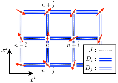
Figure 1: A schematic picture of the spin system under consideration. We assume the localized spins live on the cubic-type lattice.

In the absence of explicit symmetry-breaking terms ($D_{i}^{c}=\mu B^{a}=C^{ab}$=0), the Hamiltonian enjoys the $\mathrm{SO}(3)$ symmetry, whose possible spontaneous breaking leads to the gapless collective excitations, or magnons (quantized spin wave) as NG modes. By promoting the symmetry-breaking parameters to background fields (spurions), we can construct a low-energy effective Lagrangian for the magnons with other possible low-energy modes based only on the symmetry argument Gongyo et al. (2016). Although the explicit breaking terms break the global $\mathrm{SO}(3)$ symmetry, we can investigate their effects using the background field (or the so-called spurion) method if they are small compared to the symmetric interaction ($|D^{c}_{i}|,\,|\mu B^{a}|,\,|C^{ab}|\ll|J|$).

As the first attempt to parametrize the DM interaction, let us introduce the $\mathrm{SO}(3)$ gauge field coupled to the Noether current corresponding to the global $\mathrm{SO}(3)$ symmetry. When the Hamiltonian is given only by the first term in Eq. (1): $\hat{H}_{0}\equiv-\sum_{n,i}J(\hat{\bm{s}}^{n})^{t}\hat{\bm{s}}^{n+\hat{i}}+(\mathrm{const}.)$, the Heisenberg equation of motion for $\hat{s}_{a}^{n}$ generated by the $\mathrm{SO}(3)$ invariant Hamiltonian $\hat{H}_{0}$ provides a discretized version of the conservation law of the Noether current:

$$\partial_{t}\hat{J}^{0}_{a}(n)+\sum_{i=1}^{d}\big{[}\hat{J}^{i}_{a}(n+\hat{i}/2)-\hat{J}^{i}_{a}(n-\hat{i}/2)\big{]}=0\quad\mathrm{with}\quad\begin{cases}\hat{J}^{0}_{a}(n)\equiv\hat{s}_{a}^{n},\\ \hat{J}^{i}_{a}(n+\hat{i}/2)=J\epsilon_{a}^{~{}bc}\hat{s}_{b}^{n}\hat{s}_{c}^{n+\hat{i}}.\end{cases}$$ (2)

By introducing the background gauge field coupled to the Noether current, we obtain the following modification of the Hamiltonian:

$$\begin{split}\hat{H}_{0}&\to\hat{H}_{0}-\sum_{n}A_{0}^{a}(n)\hat{J}^{0}_{a}(n)-\sum_{n}\sum_{i=1}^{d}aA_{i}^{a}(n+\hat{i}/2)\hat{J}^{i}_{a}(n+\hat{i}/2)\\ &=-\sum_{n}\sum_{i=1}^{d}\big{[}J\delta^{ab}+JaA_{i}^{c}(n+\hat{i}/2)\epsilon_{c}^{~{}ab}\big{]}\hat{s}_{a}^{n}\hat{s}_{b}^{n+\hat{i}}-\sum_{n}A_{0}^{a}(n)\hat{s}^{n}_{a},\end{split}$$ (3)

with an $\mathrm{SO}(3)$ gauge field $A_{\mu}^{a}~{}(a=1,2,3)$. We here introduced the lattice spacing $a$ (not the $\mathrm{SO}(3)$ indices) between spins for future convenience. We can now identify two symmetry-breaking terms $\mu B^{a}$ and $D_{i}^{a}$ in the original Hamiltonian in Eq. (1) as the following background values of the $\mathrm{SO}(3)$ gauge field,

$$A_{0}^{a}(n)\equiv\mu B^{a},\quad A_{i}^{a}(n+\hat{j}/2)\equiv(Ja)^{-1}D_{i}^{a}.$$ (4)

Although this illustrates the basic idea of the background field (spurion) method for the magnetic field and the DM interaction term, this simplified Noether procedure in Eq. (3) does not implement the local $\mathrm{SO}(3)$ gauge invariance fully on the lattice and is not complete.

To correctly implement the $\mathrm{SO}(3)$ gauge invariance on the lattice, we draw an analogy to the Hamiltonian lattice gauge theory Kogut and Susskind (1975). We first make the Hamiltonian $\hat{H}_{0}$ invariant under the local $\mathrm{SO}(3)$ transformation

$$\hat{H}_{0}\to\hat{H}_{0}^{\prime}\equiv\sum_{n}\sum_{i=1}^{d}\frac{|J|}{2}\big{[}U(n,n+\hat{i})\hat{\bm{s}}^{n+\hat{i}}-\mathrm{sgn}(J)\hat{\bm{s}}^{n}\big{]}^{2}-\sum_{n}[\bm{A}_{0}(n)]^{t}\hat{\bm{s}}^{n},$$ (5)

where the local $\mathrm{SO}(3)$ transformation $g(n)\in\mathrm{SO}(3)$ acts on $\hat{\bm{s}}^{n}$, $U(n,n+\hat{i})$, and ${\bm{A}}_{0}$ as

$$\hat{\bm{s}}^{n}\to g(n)\hat{\bm{s}}^{n},\quad U(n,n+\hat{i})\to g(n)U(n,n+\hat{i})g(n+\hat{i})^{t},\quad\bm{A}_{0}(n)\to g(n){\bm{A}}_{0}.$$ (6)

Noting that the last transformation is equivalent to $A_{0}(n)\equiv A_{0}^{a}(n)t_{a}\to g(n)A_{0}g^{t}(n)$, which is identified as a time-independent gauge transformation, we will further consider time-dependent gauge invariance acting on $A_{0}(t,n)$ as

$$A_{0}(t,n)\to g(t,n)A_{0}(t,n)g(n,t)^{t}+\mathrm{i}g(t,n)^{-1}\partial_{0}g(n,t)^{t}.$$ (7)

We now study the expansion in powers of the lattice spacing $a$ of the gauge-invariant theory (5) to obtain the original Hamiltonian in Eq. (1) with symmetry-breaking terms $\mu B^{a},\,D_{i}^{a}$, and $C^{ab}$, ignoring higher-order terms in powers of $a$, which will become irrelevant in the continuum limit. By expanding the link variable $U$ at a small lattice spacing $a$, we can identify the $\mathrm{SO}(3)$ gauge field $A_{i}^{a}$ as

$$U(n,n+\hat{i})=\mathrm{e}^{\mathrm{i}aA_{i}^{a}(n+\hat{i}/2)t_{a}}=I_{3\times 3}+\mathrm{i}aA_{i}^{a}(n+\hat{i}/2)t_{a}+O(a^{2}).$$ (8)

Counting $\hat{\bm{s}}^{n+\hat{i}}+\mathrm{sgn}(J)\hat{\bm{s}}^{n}=O(a)$, the $O(a^{2})$ term in $U$ gives higher-order terms which vanish in the continuum limit. Here, we have also introduced generators of the Lie algebra $t_{a}\in\mathrm{so}(3)$ satisfying

$$[t_{a},t_{b}]=\mathrm{i}\epsilon_{ab}^{~{}~{}c}t_{c}.$$ (9)

Using the explicit form of $t_{a}$ in the vector representation:

$$t_{1}=\left(\begin{array}[]{ccc}0&0&0\\[-25.0pt] \\ 0&0&-\mathrm{i}\\[-25.0pt] \\ 0&\mathrm{i}&0\end{array}\right),\quad t_{2}=\left(\begin{array}[]{ccc}0&0&\mathrm{i}\\[-25.0pt] \\ 0&0&0\\[-25.0pt] \\ -\mathrm{i}&0&0\end{array}\right),\quad t_{3}=\left(\begin{array}[]{ccc}0&-\mathrm{i}&0\\[-25.0pt] \\ \mathrm{i}&0&0\\[-25.0pt] \\ 0&0&0\end{array}\right),$$ (10)

we expand the gauge-invariant Hamiltonian in powers of the lattice spacing $a$ as

$$\begin{split}\hat{H}_{0}^{\prime}&=\sum_{n}\sum_{i=1}^{d}\frac{|J|}{2}\left[\hat{\bm{s}}^{n+\hat{i}}-\mathrm{sgn}(J)\hat{\bm{s}}^{n}+\mathrm{i}aA_{i}^{a}t_{a}\hat{\bm{s}}^{n+\hat{i}}+O(a^{2})\right]^{2}-\sum_{n}\bm{A}_{0}\cdot\hat{\bm{s}}_{a}^{n}\\ &=\sum_{n}\sum_{i=1}^{d}\left[\frac{|J|}{2}\big{(}\hat{\bm{s}}^{n+\hat{i}}-\mathrm{sgn}(J)\hat{\bm{s}}^{n}\big{)}^{2}+Ja\bm{A}_{i}\cdot(\hat{\bm{s}}^{n+\hat{i}}\times\hat{\bm{s}}^{n})\right]-\sum_{n}\left[\bm{A}_{0}\cdot\hat{\bm{s}}_{a}^{n}-\frac{|J|a^{2}}{2}(\hat{\bm{s}}^{n})^{t}(A_{i}^{a}t_{a})^{2}\hat{\bm{s}}^{n}\right],\end{split}$$ (11)

where we have not explicitly display terms that vanish in the naive continuum limit ($O(Ja^{3})$-terms). Comparing this with the original Hamiltonian (1), we can confirm the identification (4) of the background values of the fields to obtain the magnetic field $\mu B$ and the DM interaction $D_{i}^{a}$, together with a specific value $C_{\mathrm{cr}}$ of the anisotropic potential [the last term $C$ in Eq. (1)], given by

$$C_{\mathrm{cr}}=-\frac{|J|a^{2}}{2}(A_{i}^{a}t_{a})^{2}=-\frac{1}{2|J|}(D_{i}^{a}t_{a})^{2}.$$ (12)

This fine-tuned potential corresponds to the case of the continuum Hamiltonian whose potential can be combined with the DM interaction simply as the square of the covariant derivative.

The generic values of the single-ion anisotropy $C$ can also be implemented by introducing another background scalar field $W(n)$ in the symmetric rank two tensor representation, on which the local $\mathrm{SO}(3)$ transformation $g(n)$ acts as $W(n)\to g(n)W(n)g(n)^{t}$. We should identify its background value as

$$W(n)\equiv C-C_{\mathrm{cr}}.$$ (13)

Thus, apart from higher-order terms in powers of the lattice spacing $a$, which vanish in the naïve continuum limit, we find that the Hamiltonian in Eq. (1) with symmetry-breaking terms $\mu B^{a}$, $D_{i}^{a}$ and $C^{ab}$ can be obtained from the lattice gauge invariant theory

$$\hat{H}_{0}^{\prime\prime}\equiv\sum_{n}\sum_{i=1}^{d}\frac{|J|}{2}\big{[}U(n,n+\hat{i})\hat{\bm{s}}^{n+\hat{i}}-\mathrm{sgn}(J)\hat{\bm{s}}^{n}\big{]}^{2}-\sum_{n}A_{0}^{a}(n)\hat{s}_{a}^{n}-\sum_{n}(\hat{\bm{s}}^{n})^{t}W(n)\hat{\bm{s}}^{n},$$ (14)

at particular values of the background gauge field $A_{0},\,A_{i}$ and scalar field $W$ given in Eqs. (4) and (13).

III Effective Field Theory of magnons

In this section, we implement explicit symmetry-breaking terms presented in the previous section into a field-theoretical description of spin systems, or the $\mathrm{O}(3)$ nonlinear sigma model. We also clarify the matching condition for the low-energy coefficient in the homogeneous ground state and review the low-energy spectrum in the absence of the explicit symmetry breaking (see also Appendix A for a coset construction as a complementary way to derive the effective Lagrangian).

III.1 $\mathrm{O}(3)$ nonlinear sigma model description

Since we are interested in the low-energy (long wave-length) behaviors of the system, we can employ the field-theoretical (continuum) description of the system. A continuum field-theoretical description of magnons (spin waves) is given by the $\mathrm{O}(3)$ nonlinear sigma model, in which a $3$-component unit vector $n^{a}=(n^{1},n^{2},n^{3})^{t}$ with $n^{a}n_{a}=1$ plays a role as a dynamical degree of freedom. We note that this unit vector expresses the usual magnetization order parameter in the ferromagnetic case, while it represents the Néel order parameter in the antiferromagnetic case.

The local $\mathrm{SO}(3)$ transformation simply acts on the vector field $n^{a}$ as $\bm{n}\to g(x)\bm{n}$ with $g(x)\in\mathrm{SO}(3)$ as is the case with the lattice spin. The symmetry-based discussion in the previous section enables us to incorporate explicit breaking terms in the $\mathrm{O}(3)$ nonlinear sigma model. In fact, taking the continuum limit of the background (spurious) gauge and scalar fields introduced in the previous section, we have the $\mathrm{SO}(3)$ gauge field $A_{\mu}(x)\equiv A_{\mu}(x)^{a}t_{a}$ and the scalar $W(x)$ in the symmetric tensor representation on which the local $\mathrm{SO}(3)$ transformation $g(x)\in\mathrm{SO}(3)$ acts as

$$\begin{cases}A_{\mu}(x)\to g(x)A_{\mu}(x)g^{-1}(x)+\mathrm{i}g(x)\partial_{\mu}g^{-1}(x),\\ W(x)\to g(x)W(x)g^{-1}(x).\end{cases}$$ (15)

Using these, we construct the general local $\mathrm{SO}(3)$ invariant effective Lagrangian and eventually fix the (spurious) fields to the nontrivial background values as

$$A_{0}^{a}(x)=\mu B^{a},\quad A_{i}^{a}(x)=(Ja)^{-1}D_{i}^{a}\equiv\kappa_{i}^{a},\quad W(x)=C-C_{\mathrm{cr}},$$ (16)

in order to investigate small effects of the explicit breaking terms in the lattice Hamiltonian (1).

Using the transformation rules of the fields $n^{a}(x),~{}A_{\mu}^{a}(x)$, and $W(x)$ as ingredients, we can construct the general $\mathrm{SO}(3)$ invariant effective Lagrangian. In the leading-order of the derivative expansion, where we only keep terms up to second-order in derivatives, the $\mathrm{SO}(3)$ invariant effective Lagrangian is given by

$$\mathcal{L}_{\mathrm{eff}}=\frac{m(n^{2}\partial_{0}n^{1}-n^{1}\partial_{0}n^{2})}{1+n^{3}}+mA_{0}^{a}n_{a}+\frac{f_{\rm t}^{2}}{2}(D_{0}n^{a})^{2}-\frac{f_{\rm s}^{2}}{2}(D_{i}n^{a})^{2}+\ell W^{ab}n_{a}n_{b},$$ (17)

where we defined a covariant derivative with the $\mathrm{SO}(3)$ background gauge field as

$$D_{\mu}n^{a}\equiv\partial_{\mu}n^{a}-\epsilon^{a}_{~{}bc}n^{b}A_{\mu}^{c}.$$ (18)

Equation (17) supplemented with Eq. (16) defines our effective field theory for general magnets including chiral magnets. This continuum field theory should be valid at low-energies and contains four parameters $m,f_{\rm t},f_{\rm s}$, and $\ell$ as low-energy coefficients. They can be determined from the underlying lattice model by the matching condition, which will be discussed shortly. Note that the sum of the first and second term in Eq. (17) manifestly breaks the Lorentz invariance with an effective speed of light $c_{s}\equiv f_{\rm s}/f_{\rm t}$, but is $\mathrm{SO}(3)$ gauge invariant Brauner (2010). If the symmetry-breaking terms vanish ($A^{a}_{\mu}=0,W^{ab}=0$), the effective Lagrangian in (17) reduces to the usual $\mathrm{O}(3)$ nonlinear sigma model describing ferromagnets ($m\neq 0,\,f_{\rm t}=0$), antiferromagnets $(m=0,\,f_{\rm t}\neq 0)$, and ferrimagnets ($m\neq 0,\,f_{\rm t}\neq 0$). The first term is responsible for the quadratic gapless dispersion relation of the magnon in ferro/ferrimagnets. In the rest of this section, we will introduce the matching condition and study the low-energy spectrum on the top of the homogeneous ordered phase.

III.2 Matching condition and low-energy spectrum in homogeneous order

Before discussing magnon dynamics in the presence of symmetry-breaking terms, we here clarify the matching condition for low-energy coefficients $m,f_{\rm t},f_{\rm s}$ and $\ell$ in the homogeneous ground state, which breaks approximate $\mathrm{SO}(3)$ symmetry. We also demonstrate the low-energy spectrum of gapless magnons in the absence of symmetry-breaking terms.

To illustrate the procedure in a simple context, let us assume that the symmetry-breaking background fields gives the homogeneous ground state with the magnetization/Néel vector pointing the north pole as $\langle n^{a}\rangle=n^{a}_{0}\equiv(0,0,1)^{t}$. We then introduce magnon fields $\pi^{\alpha}~{}(\alpha=1,2)$ as fluctuations on the top of the ground state, which parametrize the vector $n^{a}$ as

$$n^{a}=(\pi^{1},\pi^{2},\sqrt{1-(\pi^{\alpha})^{2}})^{t},$$ (19)

where we explicitly solved the constraint $n_{a}n^{a}=1$. Substituting this parametrization into Eq. (17), we obtain the effective Lagrangian of magnons given by

$$\mathcal{L}_{\mathrm{eff}} =-\frac{m}{2}\epsilon^{3}_{~{}\alpha\beta}\pi^{\alpha}\partial_{0}\pi^{\beta}+m\left(\delta^{3}_{a}+\epsilon^{3}_{~{}\alpha a}\pi^{\alpha}-\frac{1}{2}\delta^{3}_{a}(\pi^{\alpha})^{2}\right)A_{0}^{a}+\ell W^{33}$$

$$\quad+\frac{f_{\rm t}^{2}}{2}\delta_{\alpha\beta}D_{0}\pi^{\alpha}D_{0}\pi^{\beta}-\frac{f_{\rm s}^{2}}{2}\delta^{ij}\delta_{\alpha\beta}D_{i}\pi^{\alpha}D_{j}\pi^{\beta}-\ell\left[(W^{23}+W^{32})\pi^{1}-(W^{13}+W^{31})\pi^{2}\right]$$

$$\quad-\ell\left[(W^{33}-W^{22})(\pi^{1})^{2}+(W^{33}-W^{11})(\pi^{2})^{2}+(W^{12}+W^{21})\pi^{1}\pi^{2}\right]+\mathcal{L}_{\mathrm{int}},$$ (20)

where $\mathcal{L}_{\mathrm{int}}$ contains more than two magnon fields representing interactions between them. We have also defined the covariant derivative of the magnon field as

$$D_{\mu}\pi^{\alpha}\equiv\partial_{\mu}\pi^{\alpha}-A_{\mu}^{\alpha}-A_{\mu}^{3}\epsilon^{\alpha}_{~{}\beta 3}\pi^{\beta}.$$ (21)

Since the ground state spontaneously breaks the $\mathrm{SO}(3)$ symmetry down to its subgroup $\mathrm{SO}(2)_{z}$, the magnon fields can be identified as the NG bosons. The effective Lagrangian (20) is reparametrized by $\pi^{\alpha}$ fields in order to make their role as NG bosons manifest, and is equivalent to the original effective field theory in Eq. (17), provided all order terms of $\pi^{\alpha}$ in $\mathcal{L}_{\mathrm{int}}$ are kept. In the rest of this section, we assume symmetry-breaking terms in Eq. (20) do not induce a tachyon-like instability around the assumed ground state $n^{a}_{0}\equiv(0,0,1)^{t}$. Thus, the actual values of the symmetry-breaking terms in Eq. (20) cannot be arbitrary.

We now discuss the matching conditions within a tree-level analysis in order to fix the phenomenological parameters in the effective Lagrangian (20): the four parameters $m,~{}f_{\rm t},~{}f_{\rm s}$ and $\ell$. We first introduce the $\mathrm{SO}(3)$ current defined by the variation of the effective action $\mathcal{S}$ in terms of the $\mathrm{SO}(3)$ gauge fields

$$J^{\mu}_{a}(x)=\frac{\delta\mathcal{S}[\pi^{\alpha};A_{\mu}^{a},W]}{\delta A_{\mu}^{a}(x)}\quad\mathrm{with}\quad\mathcal{S}[\pi^{\alpha};A_{\mu}^{a},W]=\int\mathrm{d}^{d+1}x\,\mathcal{L}_{\mathrm{eff}}.$$ (22)

Up to quadratic terms in the magnon field $\pi^{\alpha}(x)$, the $SO(3)$ currents are explicitly given by

$$\begin{split}J^{0}_{3}&=m-\frac{m}{2}(\pi^{\alpha})^{2}-f_{\rm t}^{2}\epsilon_{\alpha\beta 3}\pi^{\beta}(\partial_{0}\hat{\pi}^{\alpha}-A_{0}^{\alpha}-A^{3}_{0}\epsilon^{\alpha}_{~{}\gamma 3}\pi^{\gamma})+\cdots,\\ J^{i}_{3}&=f_{\rm s}^{2}\delta^{ij}\epsilon_{\alpha\beta 3}\pi^{\beta}(\partial_{j}\pi^{\alpha}-A_{j}^{\alpha}-A^{3}_{j}\epsilon^{\alpha}_{~{}\gamma 3}\pi^{\gamma})+\cdots,\\ J^{0}_{\alpha}&=-m\epsilon^{3}_{~{}\alpha\beta}\pi^{\beta}-f_{\rm t}^{2}\delta_{\alpha\beta}(\partial_{0}\pi^{\beta}-A_{0}^{\beta}-A^{3}_{0}\epsilon^{\beta}_{~{}\gamma 3}\pi^{\gamma})+\cdots,\\ J^{i}_{\alpha}&=f_{\rm s}^{2}\delta^{ij}\delta_{\alpha\beta}(\partial_{j}\pi^{\beta}-A_{j}^{\beta}-A^{3}_{j}\epsilon^{\beta}_{~{}\gamma 3}\pi^{\gamma})+\cdots.\end{split}$$ (23)

We then define the generating functional $Z[A_{\mu}^{a},W]$ for the $\mathrm{SO}(3)$ current $J_{a}^{\mu}$ by the path integral over $\pi^{\alpha}(x)$

$$Z[A_{\mu}^{a},W]=\int\mathcal{D}\pi^{\alpha}\,\exp\left(\mathrm{i}\mathcal{S}[\pi^{\alpha};A_{\mu}^{a},W]\right).$$ (24)

The expectation values of the currents can be obtained by taking the functional derivative with respect to $A_{\mu}^{a}$

$$\langle J_{a}^{\mu}(x)\rangle=\mathrm{i}^{-1}\frac{\delta}{\delta A_{\mu}^{a}(x)}\log Z[A_{\mu}^{a},W].$$ (25)

We can also introduce the generalized susceptibility for the $\mathrm{SO}(3)$ symmetry (correlation functions of current operators), defined by

$$\chi^{\mu\nu}_{ab}(\omega,\bm{k})=-\int\mathrm{d}^{d+1}x\,\mathrm{e}^{\mathrm{i}\omega t-\mathrm{i}\bm{k}\cdot\bm{x}}\frac{\delta}{\delta A_{\mu}^{a}(x)}\frac{\delta}{\delta A_{\nu}^{b}(0)}\log Z[A_{\mu}^{a},W].$$ (26)

If we wish to find the expectation values of the current operators and the susceptibility at the tree level, we just need to evaluate Eq. (24) at the homogeneous ground state $\pi^{\alpha}(x)=0$ and the background values of $A_{\mu}^{a}$ and $W(x)$. Denoting the ground state expectation value of an operator $O$ by $\langle O\rangle$, we obtain the expectation value of the current operator $\hat{J}_{a}^{\mu}$ and the correlation functions of the current operators (susceptibility) at the tree level approximation as

$$\begin{cases}\left.\langle J_{3}^{0}(x)\rangle\right|_{\pi=0}=m,\\ \left.\chi_{\alpha\beta}^{00}(\omega=0,\bm{k}=0)\right|_{\pi=0}=f_{\rm t}^{2}\delta_{\alpha\beta},\\ \left.\chi_{\alpha\beta}^{ij}(\omega=0,\bm{k}=0)\right|_{\pi=0}=-f_{\rm s}^{2}\delta^{ij}\delta_{\alpha\beta}.\end{cases}$$ (27)

Throughout this section, we use an abbreviated notation of $\pi^{\alpha}=0$ to denote the ground state values: $\pi^{\alpha}=0$ and the background field $A_{\mu}^{a}$ and $W$ fixed at physical values given in Eq. (16). The second and third equations indicate a nonvanishing long-range correlation for the (approximately) conserved currents, which is a manifestation of spontaneous symmetry breaking. Its structure is the same as the familiar symmetry breaking in the Lorentz invariant systems, except for the independent numerical prefactor, which reflects the fact that the propagating speed of magnons is generally not the speed of light. On the other hand, the first equation is peculiar to the nonrelativistic system since the nonvanishing charge density $m\neq 0$ manifestly breaks the Lorentz invariance.

Taking the variation with respect to the background field $W$, we can also obtain the matching condition for $\ell$ as

$$\ell=\left.\Big{\langle}\frac{\delta\mathcal{S}_{\mathrm{eff}}}{\delta W^{33}}\Big{\rangle}\right|_{\pi=0},$$ (28)

which is proportional to $\langle\hat{s}_{3}^{n}\hat{s}_{3}^{n}\rangle$ in the lattice model description. Equations (27)-(28) provide the matching condition for low-energy coefficients $m,f_{\rm t},f_{\rm s}$ and $\ell$.

Depending on which coefficients are present, we can classify various magnets into three types: antiferromagnets, ferromagnets, and ferrimagnets. For simplicity, let us consider the simple situation with vanishing explicit symmetry-breaking terms—the background magnetic field $B^{a}$, DM interaction $D_{j}^{a}$, and single-ion anisotropy $C^{ab}$. In this case, we can simplify the quadratic part of the effective Lagrangian as

$$\mathcal{L}_{\mathrm{eff}}^{(2)} =-\frac{m}{2}\epsilon^{3}_{~{}\alpha\beta}\pi^{\alpha}\partial_{0}\pi^{\beta}+\frac{f_{\rm t}^{2}}{2}\delta_{\alpha\beta}\partial_{0}\pi^{\alpha}\partial_{0}\pi^{\beta}-\frac{f_{\rm s}^{2}}{2}\delta_{\alpha\beta}\delta^{ij}\partial_{i}\pi^{\alpha}\partial_{j}\pi^{\beta},$$ (29)

which results in the following equation of motion:

$$\begin{pmatrix}f_{\rm t}^{2}\partial_{0}^{2}-f_{\rm s}^{2}\bm{\nabla}^{2}&m\partial_{0}\\ -m\partial_{0}&f_{\rm t}^{2}\partial_{0}^{2}-f_{\rm s}^{2}\bm{\nabla}^{2}\end{pmatrix}\begin{pmatrix}\pi^{1}\\ \pi^{2}\end{pmatrix}=0.$$ (30)

By solving the characteristic equation for the coefficient matrix, we can investigate the number of the independent NG modes and their dispersion relations. The result is summarized as follows:

$$\begin{split}&\bullet~{}\mbox{Antiferromagnet}~{}(f_{\rm t}\neq 0,~{}m=0):~{}2\,\mbox{NG modes}\quad\mathrm{with}\quad\omega=c_{s}|\bm{k}|,\\ &\bullet~{}\mbox{Ferromagnet}~{}(f_{\rm t}=0,~{}m\neq 0)\hskip 20.0pt:~{}1\,\mbox{NG mode}\ \quad\mathrm{with}\quad\omega=\frac{f_{\rm s}^{2}}{m}\bm{k}^{2},\\ &\bullet~{}\mbox{Ferrimagnet}~{}(f_{\rm t}\neq 0,~{}m\neq 0)\hskip 22.0pt:~{}1\,\mbox{NG mode and }1\,\mbox{gapped mode}\\ &\hskip 180.0pt\mathrm{with}\quad\omega=\dfrac{f_{\rm s}^{2}}{m}\bm{k}^{2}+O(\bm{k}^{4}),\quad\omega=\dfrac{m}{f_{\rm t}^{2}}+O(\bm{k}^{2}).\end{split}$$ (31)

We list only positive frequencies here and subsequently, although there are negative frequency solutions with the opposite sign. Here, we have introduced the propagating speed of the antiferromagnetic magnon as $c_{s}\equiv f_{\rm s}/f_{\rm t}$, which is not necessarily the speed of light in contrast to the NG mode in the Lorentz invariant system. Note that the ferro/ferrimagnetic magnons show the quadratic dispersion relation, and the number of gapless excitation $N_{\mathrm{NG}}$ obeys the general counting rule

$$N_{\mathrm{NG}}=N_{\mathrm{BS}}-\mathrm{rank}\,\rho\quad\mathrm{with}\quad\rho_{ab}(x)\equiv\langle[\mathrm{i}\hat{Q}_{a},\hat{J}^{0}_{b}(x)]\rangle$$ (32)

Here, we introduced the number of the broken symmetry $N_{\mathrm{BS}}$ and the so-called Watanabe-Brauner matrix $\rho_{ab}$, where $\hat{Q}_{a}=\int\mathrm{d}^{d}x\,\hat{J}^{0}_{a}(x)~{}(a=1,2,3)$ denotes the Noether charge associated with the $\mathrm{SO}(3)$ symmetry. This result is completely consistent with the above matching condition since $\rho_{12}(x)=\langle\hat{J}^{0}_{3}(x)\rangle=m$ does not vanish in the homogeneous ferro/ferrimagnetic ground state while it does in the antiferromagnetic one. The dispersion relation at small $\bm{k}$ in the ferrimagnet case given in Eq. (31) reduces to that in the ferromagnet case as $f_{\rm t}\to 0$ while it does not reduce to that of antiferromagnet in the limit of $m\to 0$. This apparent inconsistency comes from our limiting procedure: we first take small $\bm{k}$ limit in Eq. (31) and consider $m\to 0$ limit. The full dispersion relation for ferrimagnets is available from Eq. (30), which, of course, reproduces that of antiferromagnets when we take $m\to 0$.

IV Low-energy spectrum on helical/spiral phase

In this section, we apply the effective Lagrangian (17) to study low-energy excitation spectra of inhomogeneous ground states induced by the DM interaction. When the DM interaction is sufficiently large, inhomogeneous states tend to become the ground state. The simplest of such inhomogeneous ground states develop a one-dimensional modulation of the spin vector. Depending on the types of the DM interaction, they are called the helical ground state or spiral ground state. Both of them support a gapless NG mode as a low-energy excitation, that is, the phonon associated with the spontaneous breaking of the translation symmetry. Nonetheless, we demonstrate that the form of the dispersion relation is qualitatively different between helical and spiral states.

IV.1 Isotropic dispersion relation in helical ground state

As the first application, we consider the case where the simple combination of the uniaxial DM interaction and easy-axis anisotropic potential along the same direction are present. For simplicity, we choose the following background values for the external fields in the effective Lagrangian (17):

$$A_{0}^{a}=0,\quad A_{i}^{a}=\kappa_{i}\delta^{a}_{3},\quad\mathrm{and}\quad\ell W^{ab}=\frac{W}{2}\delta^{a}_{3}\delta^{b}_{3}.$$ (33)

Using this setup, we will show that the system develops the helical order in the case of the easy-plane potential ($W<0$) Hongo et al. (2020). Due to the spontaneous breaking of the translational symmetry, the helical ground state is shown to support a translational gapless phonon (NG mode) in the low-energy spectrum irrespective of the types of chiral magnets.

In contrast to the analysis in Sec. III.2, we have an inhomogeneous ground state, which forces us to abandon the description in Eq. (20) in terms of NG bosons on the homogeneous ground state. We thus here start with the original $\mathrm{O}(3)$ nonlinear sigma model description given in Eq. (17). Substituting Eq. (33) into the effective Lagrangian (17), we obtain

$$\mathcal{L}_{\mathrm{eff}}=\frac{m(n^{2}\partial_{0}n^{1}-n^{1}\partial_{0}n^{2})}{1+n^{3}}+\frac{f_{\rm t}^{2}}{2}(\partial_{0}n^{a})^{2}-\frac{f_{\rm s}^{2}}{2}(\partial_{i}n^{a}-\kappa_{i}\epsilon^{a}_{~{}b3}n^{b})^{2}+\frac{W}{2}(n^{3})^{2}.$$ (34)

One should note that the potential $V(n^{3})=-W(n^{3})^{2}/2$ favors $n^{3}=\pm 1$ (easy-axis) if $W>0$, whereas it favors $n^{3}=0$ (easy-plane) if $W<0$. To find the ground state, we use the Hamiltonian defined by the Legendre transformation of Eq. (34) as

$$\begin{split}\mathcal{H}&=\Pi_{a}\partial_{0}n^{a}-\mathcal{L}_{\mathrm{eff}}\\ &=\frac{1}{2f_{\rm t}^{2}}\left(\Pi_{a}-\frac{m(n^{2}\delta_{a}^{1}-n^{1}\delta_{a}^{2})}{1+n^{3}}\right)^{2}+\frac{f_{\rm s}^{2}}{2}(\partial_{i}n^{a}-\kappa_{i}\epsilon^{a}_{~{}b3}n^{b})^{2}-\frac{W}{2}(n^{3})^{2}.\\ \end{split}$$ (35)

where we defined the conjugate momentum $\Pi_{a}$ as

$$\Pi_{a}\equiv\frac{\partial\mathcal{L}_{\mathrm{eff}}}{\partial(\partial_{0}n^{a})}=\frac{m(n^{2}\delta^{1}_{a}-n^{1}\delta^{2}_{a})}{1+n^{3}}+f_{\rm t}^{2}\partial_{0}n_{a}.$$ (36)

Noting that the Hamiltonian (35) is expressed as a sum of the quadratic terms, we try to find a candidate ground state solution by requiring the first two terms to vanish:

$$\partial_{0}n^{a}=0,\quad\partial_{i}n^{a}-\kappa_{i}\epsilon^{a}_{~{}b3}n^{b}=0.$$ (37)

The solutions of this set of equations are given by

$$\bar{n}^{a}=\begin{pmatrix}\sqrt{1-\bar{A}^{2}}\cos(\bm{\kappa}\cdot\bm{x}+\bar{\phi})\\ -\sqrt{1-\bar{A}^{2}}\sin(\bm{\kappa}\cdot\bm{x}+\bar{\phi})\\ \bar{A}\end{pmatrix},$$ (38)

where two real parameters $\bar{A}\in[-1,1]$ and $\bar{\phi}\in[0,2\pi)$ denote integration constants, which characterize an orbit on the unit sphere at a constant latitude $n^{3}=\bar{A}$. Since we can regard the potential to be a function of these orbits ($n_{3}=\bar{A}$), we can find the ground state by just finding the orbit corresponding to the minimum of the potential. Thus, we find the ground states as

$$\bar{A}=\left\{\begin{array}[]{c l}\pm 1&\mathrm{for}\quad W>0,\\ 0&\mathrm{for}\quad W<0,\\ \mathrm{arbitrary}\in[-1,1]&\mathrm{for}\quad W=0.\end{array}\right.$$ (39)

While the ground state is homogeneous for $\bar{A}=\pm 1$, it realizes the inhomogeneous helical order for $|\bar{A}|<1$. Figure 2 shows a schematic picture of the helical ground state configuration of $n^{a}$ with $\bar{A}=0$ (the orbit circling at the equator). Thus, we find that the helical order is realized along the direction of the DM interaction $\bm{\kappa}$ when $W\leq 0$ (see also Ref. Hongo et al. (2020)). The fine-tuned case with $W=0$ is unique in the sense that circles at any latitude give the degenerate classical ground states corresponding to the Kaplan-Shekhtman-Aharony-Entin-Wohlman limit Kaplan (1983); Shekhtman et al. (1992). In this case of $W=0$, BPS soliton solutions in ($1+1$)-dimension have been exhaustively worked out in Ref. Hongo et al. (2020). One should note that our parametrization of the $(n^{3})^{2}$ term in the potential differs from many previous works, including Ref. Hongo et al. (2020), where the additional term was present in the potential as $V(n^{3})=(-W+\bm{\kappa}^{2})(n^{3})^{2}/2$.

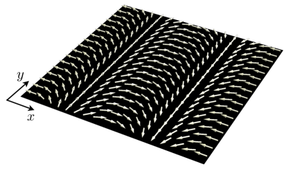
Figure 2: A schematic picture of the helical ground state in the DM dominant $(2+1)$-dimensional magnet.

Let us then consider the case with $W<0$, and investigate the low-energy spectrum on the helical ground state. For that purpose, we consider fluctuations of $\delta A$ and $\delta\phi$ around the fixed background values $\bar{A}=0$ and $\bar{\phi}=0$, and rewrite the effective Lagrangian by promoting $\delta A(x)$ and $\delta\phi(x)$ to dynamical fields. In short, we parametrize the spin vector $n^{a}$ as

$$n^{a}(x)=\begin{pmatrix}\sqrt{1-(\delta A(x))^{2}}\cos(\bm{\kappa}\cdot\bm{x}+\delta\phi(x))\\ -\sqrt{1-(\delta A(x))^{2}}\sin(\bm{\kappa}\cdot\bm{x}+\delta\phi(x))\\ \delta A(x)\end{pmatrix}\simeq\begin{pmatrix}\phantom{-}\cos(\bm{\kappa}\cdot\bm{x}+\delta\phi(x))\\ -\sin(\bm{\kappa}\cdot\bm{x}+\delta\phi(x))\\ \delta A(x)\end{pmatrix},$$ (40)

where, in the second equality, we have retained the leading order of the expansion with respect to the fluctuation ($\delta A$ and $\delta\phi$) to investigate the low-energy spectra of $\delta A$ and $\delta\phi$. Substituting this parametrization into the original effective Lagrangian (34), we now obtain the quadratic part of the Lagrangian for the amplitude mode $\delta A$ and phase mode $\delta\phi$ as

$$\begin{split}\mathcal{L}_{\mathrm{eff}}^{(2)}&=m(1-\delta A)\partial_{0}\delta\phi+\frac{f_{\rm t}^{2}}{2}[(\partial_{0}\delta A)^{2}+(\partial_{0}\delta\phi)^{2}]-\frac{f_{\rm s}^{2}}{2}[(\partial_{i}\delta A)^{2}+(\partial_{i}\delta\phi)^{2}]+\frac{W}{2}(\delta A)^{2},\end{split}$$ (41)

from which we can read off the following linearized equations of motion:

$$\begin{pmatrix}f_{\rm t}^{2}\partial_{0}^{2}-f_{\rm s}^{2}\bm{\nabla}^{2}&-m\partial_{0}\\ m\partial_{0}&f_{\rm t}^{2}\partial_{0}^{2}-f_{\rm s}^{2}\bm{\nabla}^{2}-W\end{pmatrix}\begin{pmatrix}\delta\phi\\ \delta A\end{pmatrix}=0.$$ (42)

Note that the equations of motion for the amplitude and phase fluctuations are coupled in the presence of the magnetization parameter $m$ while they decouple for vanishing $m$. Solving the characteristic equation for the matrix and noting $W=-|W|$, we obtain the dispersion relation in each case of magnets as
$\bullet~{}\mbox{Antiferromagnet}~{}(f_{\rm t}\neq 0,~{}m=0):$

$$\omega~{}=~{}\frac{f_{\rm s}}{f_{\rm t}}|\bm{k}|,\quad\frac{\sqrt{|W|+(f_{\rm s}\bm{k})^{2}}}{f_{\rm t}},$$ (43)

$\bullet~{}\mbox{Ferromagnet}~{}(f_{\rm t}=0,~{}m\neq 0):$

$$\omega~{}=~{}\frac{f_{\rm s}|\bm{k}|\sqrt{|W|+(f_{\rm s}\bm{k})^{2}}}{m},$$ (44)

$\bullet~{}\mbox{Ferrimagnet}~{}(f_{\rm t}\neq 0,~{}m\neq 0):~{}$

$$\omega~{}=~{}\begin{cases}\left(\dfrac{|W|}{m^{2}+|W|}\right)^{\frac{1}{2}}\dfrac{f_{\rm s}}{f_{\rm t}}|\bm{k}|+\dfrac{m^{4}}{2\sqrt{|W|(m^{2}+|W|)^{5}}}\dfrac{\left(f_{\rm s}|\bm{k}|\right)^{3}}{f_{\rm t}}+O(|\bm{k}|^{5}),\vspace{5pt}\\ \dfrac{\sqrt{m^{2}+|W|}}{f_{\rm t}}+\dfrac{2m^{2}+|W|}{2(m^{2}+|W|)^{3/2}}\dfrac{f_{\rm s}^{2}\bm{k}^{2}}{f_{\rm t}}+O(\bm{k}^{4}).\\ \end{cases}$$ (45)

We now see that the system supports only one gapless excitation (NG mode), and its dispersion relation is linear with respect to the momentum in all cases, in contrast to the case of $W=0$ in Eq. (45).

In the current case ($W<0$), the dispersion relation at small $\bm{k}$ in the ferrimagnet case (45) reduces to that in the antiferromagnet case (43) in the limit of $m\to 0$, but does not reduce to that in the ferromagnet case of (44) in the limit of $f_{\rm t}\to 0$. On the other hand, the dispersion relations for antiferromagnet in Eq. (43) and ferromagnet in Eq. (44) reduce in the limit $W\to 0$ to Eq. (31) for anti-ferromagnet and ferromagnet. However, the dispersion relation of the gapless mode of ferrimagnet in Eq. (45) is singular as $W\to 0$ and does not agree with Eq. (31). This discontinuity is due to the change of the small $\bm{k}$ behavior from $|W||\bm{k}|$ at $W<0$ to $\bm{k}^{2}$ at $W=0$, which is similar to magnon dispersion relations in the homogeneous ordered phase. Again, the full dispersion relation for ferrimagnets before small-$\bm{k}$ expansion, which is available from solving (42), reproduces both ferromagnetic and antiferromagnetic limits.

One may regard this gapless mode as the translational phonon. However, we note that it is also possible to interpret this mode as the magnon mode in a “rotating frame”. This is because one can eliminate the DM interaction by performing the field redefinition of the spin vector (see e.g., Ref. Hongo et al. (2020)). As a result, the newly defined spin develops the homogeneous order so that one obtains the corresponding magnon mode. In this interpretation, the linear dispersion with $W<0$ corresponds to the magnon in the presence of the easy-plane potential, where the remaining $\mathrm{SO}(2)$ symmetry is spontaneously broken (the spectrum with $W=0$ corresponds to the magnon without $\mathrm{SO}(3)$ symmetry breaking perturbations).

IV.2 Anisotropic dispersion relation in spiral ground state

Let us next consider the $(2+1)$-dimensional chiral magnets containing an isotropic (in the $x,y$ plane) DM interaction $D_{i}^{a}\propto\delta_{i}^{a},~{}i=1,2$, which allows a spiral ground state when the DM interaction is more dominant than the potential. In order to obtain the simplest explicit solution, we consider the case without a potential (after the DM interactions are explicitly separated from covariant derivatives). Hence our effective Lagrangian is given by

$$\mathcal{L}_{\mathrm{eff}}=\frac{m(n^{2}\partial_{0}n^{1}-n^{1}\partial_{0}n^{2})}{1+n^{3}}+\frac{f_{\rm t}^{2}}{2}(\partial_{0}n^{a})^{2}-\frac{f_{\rm s}^{2}}{2}(\partial_{i}n^{a})^{2}+f_{\rm s}^{2}\kappa\big{[}n^{3}(\partial_{y}n^{1}-\partial_{x}n^{2})+(n^{2}\partial_{x}-n^{1}\partial_{y})n^{3}\big{]}.$$ (46)

This Lagrangian corresponds to the following choice of background fields with a constant term $-\kappa^{2}/2$ discarded:

$$A_{0}^{a}=0,\quad A_{i}^{a}=-\kappa\delta_{i}^{a},\quad\ell W_{ab}n^{a}n^{b}=-f_{\rm s}^{2}\kappa^{2}(n^{3})^{2}.$$ (47)

Instead of treating the constrained variable $n^{a}$, we now explicitly solve the constraint $n^{a}n_{a}=1$ by using the spherical parameterization of the spin vector $n^{a}$ given by

$$n^{a}=(\sin\theta\cos\phi,\sin\theta\sin\phi,\cos\theta)^{t}\quad\mathrm{with}\quad 0\leq\theta<\pi,\quad 0\leq\phi<2\pi.$$ (48)

Substituting this into Eq. (46), we obtain the Lagrangian in terms of the unconstrained variables

$$\begin{split}\mathcal{L}_{\mathrm{eff}}=&2m\sin^{2}\frac{\theta}{2}\partial_{0}\phi+\frac{f_{\rm t}^{2}}{2}\big{[}(\partial_{0}\theta)^{2}+\sin^{2}\theta(\partial_{0}\phi)^{2}\big{]}-\frac{f_{\rm s}^{2}}{2}\big{[}(\partial_{i}\theta)^{2}+\sin^{2}\theta(\partial_{i}\phi)^{2}\big{]}\\ &+f_{\rm s}^{2}\kappa\Big{[}(\cos\phi\partial_{y}-\sin\phi\partial_{x})\theta-\frac{1}{2}\sin 2\theta(\cos\phi\partial_{x}+\sin\phi\partial_{y})\phi\Big{]}.\end{split}$$ (49)

To find a one-dimensionally inhomogeneous solution, let us assume that the configuration is independent of time $t$ and spatial coordinate $y$. This assumption is consistent with the equation of motion, thanks to the spacetime translational symmetry. Retaining only the $x$-dependence, we find energy density ${\cal E}$ of such a configuration as

$${\cal E}[\theta,\phi]=\frac{f_{\rm s}^{2}}{2}\left[\left(\frac{\mathrm{d}\theta}{\mathrm{d}x}\right)^{2}+\sin^{2}\theta\left(\frac{\mathrm{d}\phi}{\mathrm{d}x}\right)^{2}\right]-f_{\rm s}^{2}\kappa\left[-\sin\phi\frac{\mathrm{d}\theta}{dx}-\frac{1}{2}\sin 2\theta\cos\phi\frac{\mathrm{d}\phi}{\mathrm{d}x}\right].$$ (50)

The equation of motion for $\phi$ can be solved trivially by taking

$$\phi=\pm\frac{\pi}{2}+2n\pi,\quad n\in Z.$$ (51)

With this choice, the energy density becomes

$${\cal E}[\theta]=\frac{f_{\rm s}^{2}}{2}\left(\frac{\mathrm{d}\theta}{\mathrm{d}x}\right)^{2}\pm f_{\rm s}^{2}\kappa\frac{\mathrm{d}\theta}{\mathrm{d}x},$$ (52)

where $\pm$ sign corresponds to $\phi=\pm\pi/2+2n\pi$. It is interesting to observe that the DM interaction for the one-dimensionally inhomogeneous configuration becomes a total derivative and does not affect the equation of motion for $\theta$, which becomes

$$\frac{\mathrm{d}^{2}\bar{\theta}(x)}{\mathrm{d}x^{2}}=0,$$ (53)

yielding the following solution:

$$\bar{\theta}(x)=cx+d\quad\mathrm{with}\quad c,d\in\mathbb{R},$$ (54)

where $c$ and $d$ are integration constants. Although all these solutions with arbitrary values of $c,d$ are solutions of the field equations, they can give different energy density because of the total derivative term induced by the DM interaction. We can minimize the energy density of these solutions

$${\cal E}[\bar{\theta}]=f_{\rm s}^{2}\left(\frac{c^{2}}{2}\pm\kappa c\right),$$ (55)

to find the ground state at the value of $c=\mp\kappa$. Since both signs give physically equivalent ground state, we find the spiral ground state with a moduli parameter $d$ as

$$\bar{\phi}=\frac{\pi}{2},\quad\bar{\theta}(x)=-\kappa x+d,\quad\mathrm{with}\quad d\in\mathbb{R}.$$ (56)

Since this ground state solution represents the one-dimensional spiral modulation of the spin vector, it is called the spiral phase (see Fig. 3). The most general spiral solution can be obtained by applying simultaneous rotation in the $x$-$y$ plane and spin vector in the $n^{1}$-$n^{2}$ plane. The spiral state is similar to the helical state in that both describe the one-dimensional modulations. Nevertheless, the behavior of the collective excitation, or the translational phonon, is qualitatively different, as will be shown below. As a representative spiral state, we take the solution in Eq. (56) as the background to study the dispersion relation of low-energy excitations.

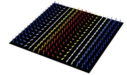
Figure 3: A schematic picture of the spiral ground state in the $(2+1)$-dimensional magnet.

To investigate the low-energy excitation in the spiral ground state, we introduce the fluctuations $\delta\theta$ and $\delta\phi$ around the helical ground state as

$$\theta(t,\bm{x})=-\kappa x+\delta\theta(t,\bm{x}),\quad\phi(t,\bm{x})=\frac{\pi}{2}+\delta\phi(t,\bm{x}).$$ (57)

Then, we substitute this parametrization to the effective Lagrangian (49) and collect the terms within the quadratic order of fluctuations. We find that it is useful to use $\delta\Omega(x)\equiv\sin(-\kappa x)\delta\phi$ instead of $\delta\phi(x)$. The resulting effective Lagrangian for the fluctuations $\delta\theta$ and $\delta\Omega$ is given by

$$\begin{split}\mathcal{L}_{\mathrm{eff}}^{(2)}=&\frac{f_{\rm t}^{2}}{2}\big{[}(\partial_{0}\delta\theta)^{2}+(\partial_{0}\delta\Omega)^{2}\big{]}-\frac{f_{\rm s}^{2}}{2}\big{[}(\partial_{i}\delta\theta)^{2}+(\partial_{i}\delta\Omega)^{2}\big{]}-\frac{f_{\rm s}^{2}\kappa^{2}}{2}(\delta\Omega)^{2}\\ &+m\delta\theta\partial_{0}\delta\Omega-2f_{\rm s}^{2}\kappa\sin\kappa x\,\delta\theta\partial_{y}\delta\Omega.\end{split}$$ (58)

This result shows that the fluctuations $\delta\theta$ and $\delta\Omega$ couple through the first-order time derivative term, and the sinusoidal modulation proportional to the magnitude of the DM interaction $\kappa$ with the momentum $\partial_{y}$ perpendicular to the modulation. Due to the explicit presence of the sinusoidal function, the linear mode analysis will be a little complicated in the same way as the band theory with a periodic potential.

Let us investigate the low-energy spectrum described by Eq. (58). First of all, we derive the equation of motion given by

$$\begin{split}f_{\rm t}^{2}\partial_{0}^{2}\delta\theta-m\partial_{0}\delta\Omega-f_{\rm s}^{2}\bm{\nabla}^{2}\delta\theta+2f_{\rm s}^{2}\kappa\sin\kappa x\partial_{y}\delta\Omega&=0,\\ f_{\rm t}^{2}\partial_{0}^{2}\delta\Omega+m\partial_{0}\delta\Omega-f_{\rm s}^{2}\bm{\nabla}^{2}\delta\Omega+f_{\rm s}^{2}\kappa^{2}\delta\Omega-2f_{\rm s}^{2}\kappa\sin\kappa x\partial_{y}\delta\theta&=0.\end{split}$$ (59)

Performing the Fourier transformation with respect to the time argument, we can rewrite these equations in a matrix form:

$$A(\omega)\vec{\varphi}=H(x)\vec{\varphi}\quad\mathrm{with}\quad\vec{\varphi}\equiv\begin{pmatrix}\delta\theta\\ \delta\Omega\end{pmatrix},$$ (60)

where we introduced the coefficient matrices as

$$A(\omega)\equiv\begin{pmatrix}f_{\rm t}^{2}\omega^{2}&-\mathrm{i}m\omega\\ \mathrm{i}m\omega&f_{\rm t}^{2}\omega^{2}\end{pmatrix}\quad\mathrm{and}\quad H(x)\equiv f_{\rm s}^{2}\begin{pmatrix}-\bm{\nabla}^{2}&2\kappa\sin\kappa x\partial_{y}\\ -2\kappa\sin\kappa x\partial_{y}&-\bm{\nabla}^{2}+\kappa^{2}\end{pmatrix}.$$ (61)

Let us first derive the eigenvalue spectra of the reduced Hamiltonian $H(x)$, which are periodic along the $x$-direction as $x\to x+a$ with the period $a\equiv 2\pi/\kappa$. Thanks to the periodicity, we can apply the Bloch’s theorem Bloch (1929), by introducing $\vec{\varphi}_{k}$ as a simultaneous eigenstate for $H$ and the discrete translation $T_{a}=\mathrm{e}^{a\partial_{x}}$ as

$$H(x)\vec{\varphi}_{k_{x}}(x)=E_{k_{x}}\vec{\varphi}_{k_{x}}(x)\quad\mathrm{and}\quad T_{a}\vec{\varphi}_{k_{x}}(x)=\mathrm{e}^{\mathrm{i}k_{x}a}\vec{\varphi}_{k_{x}}(x).$$ (62)

Here, the discrete translation operator induces $T_{a}H(x+a)T_{a}^{-1}=H(x)$ and $T_{a}\vec{\varphi}(x)=\vec{\varphi}(x+a)$. The Bloch’s theorem tells us that we can decompose such an eigenvector as

$$\vec{\varphi}_{k_{x}}(x)=\int\frac{\mathrm{d}k_{\perp}}{2\pi}\sum_{n}\mathrm{e}^{\mathrm{i}(k_{x}+\kappa n)x+\mathrm{i}k_{\perp}y}\vec{v}_{n}(\bm{k}),$$ (63)

with $\vec{v}_{n}(\bm{k})\equiv(v_{n}^{(0)}(\bm{k}),v_{n}^{(1)}(\bm{k}))^{t}$. We also have introduced the momentum perpendicular to the modulation direction as $k_{\perp}$. Note that the momentum along the modulation direction $k_{x}$ takes a value within the first Brillouin zone: $k_{x}\in[-\pi/a,\pi/a)=[-\kappa/2,\kappa/2)$. Substituting this vector into the eigenvalue problem, we obtain recurrence relations among $v_{n}$ as

$$\begin{split}f_{\rm s}^{2}\left([(k_{x}+\kappa n)^{2}+k_{\perp}^{2}]v_{n}^{(0)}(\bm{k})+\kappa k_{\perp}[v_{n-1}^{(1)}(\bm{k})-v_{n+1}^{(1)}(\bm{k})]\right)&=E_{n}(\bm{k})v_{n}^{(0)}(\bm{k}),\\ f_{\rm s}^{2}\left(-\kappa k_{\perp}[v_{n-1}^{(0)}(\bm{k})-v_{n+1}^{(0)}(\bm{k})]+[(k_{x}+\kappa n)^{2}+k_{\perp}^{2}+\kappa^{2}]v_{n}^{(1)}(\bm{k})\right)&=E_{n}(\bm{k})v_{n}^{(1)}(\bm{k}).\end{split}$$ (64)

As is expected, the nondiagonal element is proportional to $\kappa k_{\perp}$. Thus, we can derive the exact result for the eigenvalue with the eigenfunction on the momentum plane $k_{\perp}=0$ as

$$E_{n}^{(0)}(k_{x},0)=f_{\rm s}^{2}(k_{x}+\kappa n)^{2}\quad\mathrm{and}\quad E_{n}^{(1)}(k_{x},0)=f_{\rm s}^{2}[(k_{x}+\kappa n)^{2}+\kappa^{2}].$$ (65)

It is clear that the former branch of the solution with $n=0$ gives the lowest-lying eigenvalue, and all the bands with $n\neq 0$ have the gaps determined by the magnitude of the DM interaction $\kappa$.

Apart from the $k_{\perp}=0$ plane, we need to solve the coupled infinite-dimensional recurrence relation. We observe that the coupling between neighboring bands $n$ and $n+1$ is proportional to $\kappa k_{\perp}$, and that the recurrence relations separate into two sets: those relating $v_{2n}^{(0)}$ with $v_{2n+1}^{(1)}$ and those relating $v_{2n}^{(1)}$ with $v_{2n+1}^{(0)}$. These facts allow us to use an approximation to take account of only $2n+1$ bands between the $-n$-th and $n$-th bands, in order to obtain eigenvalues of the Hamiltonian at small $\bm{k}^{2}/\kappa^{2}$ for low-lying states. Defining $\omega^{+}_{n}\equiv(k_{x}+n\kappa)^{2}+k_{\perp}^{2}+\kappa^{2}$ and $\omega^{-}_{n}\equiv(k_{x}+n\kappa)^{2}+k_{\perp}^{2}$, we find an explicit form of the eigenvalue problem in the three-band truncated approximation as the following two sets of $3\times 3$ matrix equations

$$\begin{pmatrix}\omega_{1}^{+}-\frac{E(\bm{k})}{f_{\rm s}^{2}}&-\kappa k_{\perp}&0\\ -\kappa k_{\perp}&\omega_{0}^{-}-\frac{E(\bm{k})}{f_{\rm s}^{2}}&\kappa k_{\perp}\\ 0&\kappa k_{\perp}&\omega_{-1}^{+}-\frac{E(\bm{k})}{f_{\rm s}^{2}}\\ \end{pmatrix}\begin{pmatrix}v_{1}^{(1)}(\bm{k})\\ v_{0}^{(0)}(\bm{k})\\ v_{-1}^{(1)}(\bm{k})\\ \end{pmatrix}=0,$$ (66)

$$\begin{pmatrix}\omega_{1}^{-}-\frac{E(\bm{k})}{f_{\rm s}^{2}}&\kappa k_{\perp}&0\\ \kappa k_{\perp}&\omega_{0}^{+}-\frac{E(\bm{k})}{f_{\rm s}^{2}}&-\kappa k_{\perp}\\ 0&-\kappa k_{\perp}&\omega_{-1}^{-}-\frac{E(\bm{k})}{f_{\rm s}^{2}}\\ \end{pmatrix}\begin{pmatrix}v_{1}^{(0)}(\bm{k})\\ v_{0}^{(1)}(\bm{k})\\ v_{-1}^{(0)}(\bm{k})\\ \end{pmatrix}=0.$$ (67)

We find discrete energy bands $E_{n}(\bm{k})$ labeled by $n=0,1,2,\cdots$, as a function of momentum $\bm{k}$ in the first Brillouin zone, by solving the third-order equations for vanishing determinant of the three-band equations. Similarly, we can also consider five-band truncated approximation. The ground state eigenvalue in the five-band approximation is obtained by solving the following $5\times 5$ matrix equations

$$\begin{pmatrix}\omega_{2}^{+}-\frac{E(\bm{k})}{f_{\rm s}^{2}}&-\kappa k_{\perp}&0&0&0\\ \kappa k_{\perp}&\omega_{1}^{+}-\frac{E(\bm{k})}{f_{\rm s}^{2}}&-\kappa k_{\perp}&0&0\\ 0&-\kappa k_{\perp}&\omega_{0}^{-}-\frac{E(\bm{k})}{f_{\rm s}^{2}}&\kappa k_{\perp}&0\\ 0&0&\kappa k_{\perp}&\omega_{-1}^{+}-\frac{E(\bm{k})}{f_{\rm s}^{2}}&-\kappa k_{\perp}\\ 0&0&0&\kappa k_{\perp}&\omega_{-2}^{+}-\frac{E(\bm{k})}{f_{\rm s}^{2}}\\ \end{pmatrix}\begin{pmatrix}v_{2}^{(0)}(\bm{k})\\ v_{1}^{(1)}(\bm{k})\\ v_{0}^{(0)}(\bm{k})\\ v_{-1}^{(1)}(\bm{k})\\ v_{-2}^{(0)}(\bm{k})\\ \end{pmatrix}=0.$$ (68)

Figure 4 shows the comparison of the eigenvalues $E_{n}(0,k_{\perp})$ with the three-band and five-band approximations. Note that while the results for the three-band approximation (dashed lines) and five-band approximation (solid lines) are not so different at the low-$k_{\perp}$ region and the low-lying band, the deviation appears at high-$k_{\perp}$ regions and at higher bands. As we increase the number of bands in the approximation, we, of course, obtain more bands of eigenvalues. We are interested in the dispersion relation at small values of momentum, especially for low-lying states. Because the coupling between neighboring bands is proportional to $k_{\perp}/\kappa$, we can use an expansion in powers of $k_{\perp}/\kappa$ to evaluate energy eigenvalues. We find that the $(2n+1)$-band approximation gives an exact result for the lowest-band spectrum $E_{0}(\bm{k})/(f_{\rm s}^{2}\kappa^{2})$ up to terms of order $(k_{\perp}/\kappa)^{2n}$ in powers of $(k_{\perp}/\kappa)^{2}$.

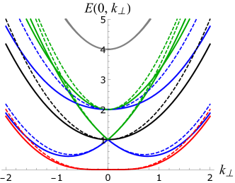
Figure 4: A comparison of the eigenvalue $E(0,k_{\perp})$ with the $3$-band approximation (dashed lines) vs $5$-band approximation (solid lines) on the $k_{x}=0$ plane ($\kappa=1$).

Once eigenvalues of the reduced Hamiltonian $H$ are given in terms of the band energy spectra $E_{n}(\bm{k})$ in the momentum space with the corresponding eigenvector $\vec{\varphi}_{n}$, we can obtain the dispersion relation by solving the following equation [recall Eqs. (60)-(61)]:

$$\begin{pmatrix}f_{\rm t}^{2}\omega^{2}-E_{n}(\bm{k})&-\mathrm{i}m\omega\\ \mathrm{i}m\omega&f_{\rm t}^{2}\omega^{2}-E_{n}(\bm{k})\end{pmatrix}\vec{\varphi}_{n}=0.$$ (69)

To find nontrivial eigenvectors, we require the determinant of the coefficient matrix to vanish. This characteristic equation gives the dispersion relations given by

$$\begin{split}&\bullet~{}\mbox{Antiferromagnet}~{}(f_{\rm t}\neq 0,~{}m=0):~{}\omega_{n}(\bm{k})=\frac{\sqrt{E_{n}(\bm{k})}}{f_{\rm t}}=c_{s}\frac{\sqrt{E_{n}(\bm{k})}}{f_{\rm s}}\quad(2~{}\mathrm{modes}),\vspace{5pt}\\ &\bullet~{}\mbox{Ferromagnet}~{}(f_{\rm t}=0,~{}m\neq 0):~{}\hskip 19.91692pt\omega_{n}(\bm{k})=\dfrac{E_{n}(\bm{k})}{m}\quad(1~{}\mathrm{mode}),\vspace{5pt}\\ &\bullet~{}\mbox{Ferrimagnet}~{}(f_{\rm t}\neq 0,~{}m\neq 0):~{}\hskip 22.76219pt\omega_{n}(\bm{k})=\dfrac{\sqrt{m^{2}+4f_{\rm t}^{2}E_{n}(\bm{k})}\pm m}{2f_{\rm t}^{2}}\quad(2~{}\mathrm{modes}),\end{split}$$ (70)

where we again introduced $c_{s}\equiv f_{\rm s}/f_{\rm t}$. As is the case for the homogeneous ground state, the number of the independent modes for ferromagnets ($f_{\rm t}\neq 0,~{}m=0$) is half of that of the antiferromagnets ($f_{\rm t}=0,~{}m\neq 0$) or ferrimagnets ($f_{\rm t}\neq 0,~{}m\neq 0$). This is because the vanishing $f_{\rm t}^{2}$ makes two fluctuation components $\delta\theta$ and $\delta\Omega$ to be one canonically conjugate pair of dynamical variables so that they just give one independent degree of freedom in contrast to the case of other magnets, where they become two independent degrees.

Equation (70) enables us to clarify the low-energy spectrum of the spiral phase from the approximated eigenvalue $E_{n}(k_{x},k_{\perp})$. The resulting dispersion relations with the five-band approximation are shown in Figs. 5-8 (note that $k_{x}$ takes the value in $k_{x}\in[-\kappa/2,\kappa/2)$ while $k_{\perp}$ can be any real number $k_{\perp}\in\mathbb{R}$). One sees that the lowest branch of the bands ($n=0$) gives the gapless excitation, which dominates the low-energy behavior of the spiral phase. Besides, we also have other bands ($n=\pm 1,\pm 2$ in the current working accuracy) corresponding to the gapped excitation in the first Brillouin zone: $k_{x}\in[-\kappa/2,\kappa/2)$. Recall that the number of the independent mode is different as shown in Eq. (70): all the spectra for the antiferromagnetic case ($f_{\rm t}\neq 0,~{}m=0$) are doubly degenerated, and the ferrimagnetic case ($f_{\rm t}\neq 0,~{}m\neq 0$) breaks that degeneracy, so that more surfaces can be seen in the leftmost panels of Figs. 7-8.

The rightmost panel in Figs 5-8 shows the section of the low-energy spectrum at $k_{x}=0$ and $k_{\perp}=0$, respectively. In sharp contrast to the helical phase, the fluctuation spectrum at the low-energy region shows anisotropic behaviors. This peculiar behavior results from the anisotropic behavior of the eigenvalue $E_{n=0}(k_{x},k_{\perp})$:

$$E_{n=0}(k_{x},k_{\perp})=k_{x}^{2}-\frac{k_{x}^{2}k_{\perp}^{2}}{\kappa^{2}}+\frac{3k_{\perp}^{4}}{8\kappa^{2}}+\cdots,$$ (71)

which is exact up to the order of $k_{\perp}^{4}$ in powers of $k_{\perp}/\kappa$, and can be obtained in the five-band approximation in Eq. (68).

Using Eq. (70), we find the low-energy spectrum for the spiral phase. Depending on the type of magnets, we find the dispersion relation for the lowest (gapless) mode as follows

• Antiferromagnet:

  $$\omega_{n=0}(\bm{k})=\begin{cases}c_{s}|k_{x}|\left(1-\dfrac{k_{\perp}^{2}}{2\kappa^{2}}+\dfrac{3k_{\perp}^{4}}{16\kappa^{2}|k_{x}|^{2}}+\cdots\right)\quad\mathrm{if}\;k_{x}\not=0,\;\;\vspace{3pt}\\ c_{s}\sqrt{\dfrac{3}{8}}\dfrac{k_{\perp}^{2}}{\kappa}+\cdots\quad\mathrm{if}\;k_{x}=0,\end{cases}$$ (72)

• Ferromagnets or Ferrimagnets:

  $$\omega_{n=0}(\bm{k})=\dfrac{f_{\rm s}^{2}}{m}\left[k_{x}^{2}\left(1-\frac{k_{\perp}^{2}}{\kappa^{2}}\right)+\frac{k_{\perp}^{4}}{2\kappa^{2}}+\cdots\right].$$ (73)

This gapless excitation is identified as the NG mode associated with the spontaneous symmetry breaking of the one-dimensional translation. The anisotropic dispersion relation is a remarkable property of the one-dimensional modulation consistent with the result from a symmetry-based general approach Hidaka et al. (2015). We also note that ferrimagnets have another branch of the gapped mode, whose gap is controlled by the magnetization parameter $m$. Thus, the gapped mode can appear with a relatively small gap when $m/(f_{\rm s}f_{\rm t}\kappa)<1$ (compare Fig. 7 and Fig. 8).

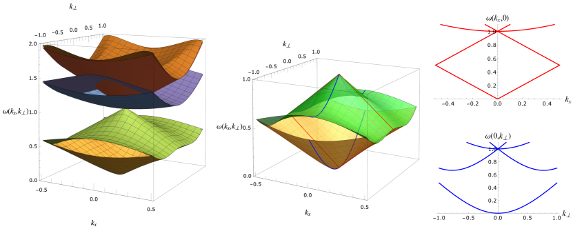
Figure 5: Low-energy spectrum for the antiferromagnetic spiral phase with the $5$-band approximation ($\kappa=1,~{}f=1$).

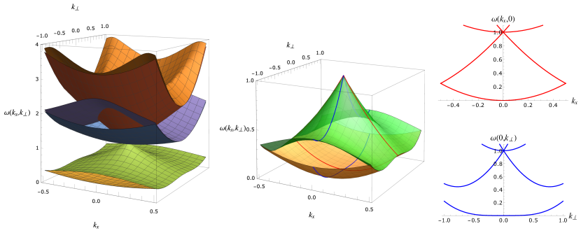
Figure 6: Low-energy spectrum for the ferromagnetic spiral phase with the $5$-band approximation ($\kappa=1,~{}m=1$).

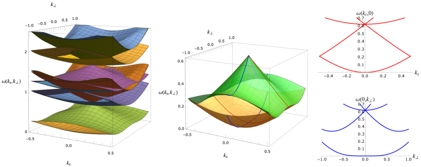
Figure 7: Low-energy spectrum for the ferrimagnetic spiral phase with the $5$-band approximation ($\kappa=1,~{}f^{2}=1,~{}m=0.5$).

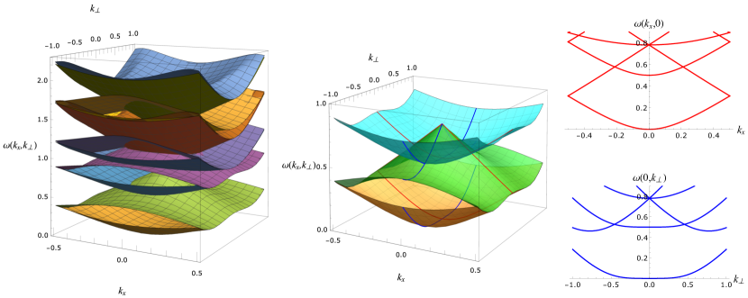
Figure 8: Low-energy spectrum for the ferrimagnetic spiral phase with the $5$-band approximation ($\kappa=1,~{}f^{2}=1,~{}m=1$).

A remark on the possible breakdown of the long-range order is in order. Due to its peculiar low-$k_{\perp}$ behavior of the dispersion relation—quadratic for antiferromagnet and quartic for ferro/ferrimagnets—one may wonder whether it does affect the fate of the spiral phase to be disordered or to be the quasi-long range order. At zero temperature, we may not encounter with an infrared divergence for the correlation function of NG modes thanks to the frequency (and $k_{x}$) integral. In particular, the zero-temperature ferro/ferrimagnets are free from such a dangerous fluctuation contribution because one finds no contribution after performing frequency integral. This situation is similar to the fact that the Mermin-Wagner theorem Mermin and Wagner (1966); Hohenberg (1967); Coleman (1973) does not apply to the zero-temperature $(1+1)$-dimensional ferromagnet. Nevertheless, in the finite-temperature systems, all magnets could suffer from the divergent fluctuation contribution, so that they may develop the quasi-long range order (or may be disordered) instead of the true long-range order (see e.g., Chaikin and Lubensky (2000)). It is interesting to investigate the fate of the spiral phase at the finite-temperature, but it is beyond the scope of this paper.

Before closing this section, we comment on the degenerate point in the spectrum. As we learn at the beginning of the band theory, the band crossing is usually avoided because of the level repulsion, which results from nondiagonal matrix elements of the involving energy states. However, as is shown in Figs. 5-8, we find several crossing points at the higher bands. This is because every band in the current model only couples to their nearest neighboring bands so that no level repulsion takes place between non-nearest neighbors. In that sense, most of the degenerate points appear just accidentally. However, there is a special degenerate point $(k_{x},k_{\perp})=(\pm\kappa/2,0)$ located at the boundary of the Brillouin zone, where all bands show two-fold degeneracy. This two-fold degeneracy has a simple origin: first, there is no coupling between different bands when $k_{\perp}=0$, so that the $k_{x}$ spectrum on the $k_{\perp}=0$ plane is continuous as given in Eq. (65). Second, the $k_{x}$ spectrum has to live within the first Brillouin zone, because of the periodicity in the $x$ direction. Therefore, the two-fold degeneracy at $(k_{x},k_{\perp})=(\pm\kappa/2,0)$ is inevitable.

V Magnon production by inhomogeneous magnetic field

In this section, we consider the production rate of magnons from the homogeneous ground state in $(d+1)$-dimensions caused by an inhomogeneous magnetic field, as another application of the effective field theory of magnons. This mechanism gives a magnon analogue of a pair creation of charged particles by an electric field—the Schwinger mechanism Schwinger (1951). We show that the magnon production rate (or ground state decay rate) is controlled by an “effective mass” of the magnon consisting of the quadratic term of the potential and the ratio of the coefficients of the linear and quadratic time derivative terms. Hence, we will find different types of magnets (ferro-, antiferro-, ferrimagnets) give drastically different magnon production rates.

Suppose that our spin system possesses a potential with an easy-axis anisotropy and develops the homogeneous ground state. In addition, we apply an inhomogeneous magnetic field along the spin direction of the ground state and investigate the resulting dynamics of magnons. We also assume for simplicity that there is no DM interaction. This situation is described by the effective Lagrangian with the following background values of the external fields:

$$A_{0}^{a}=\mu B(x)\delta^{a}_{3},\quad A_{i}^{a}=0,\quad\mathrm{and}\quad\ell W^{ab}=\frac{M^{2}}{2}\delta^{a}_{3}\delta^{b}_{3},$$ (74)

with $M^{2}>0$ (easy-axis). We also assume the sign of the background magnetic field as $B(x)\geq 0$, so that the ground state is fixed as $n^{a}=(0,0,1)^{t}$. Substituting these background values into the effective Lagrangian (20), we obtain the effective Lagrangian at the quadratic order of fluctuation fields $\pi^{\alpha}~{}(\alpha=1,2)$ around the ground state $\langle n^{a}\rangle=(0,0,1)^{t}$ as

$$\begin{split}\mathcal{L}^{(2)}&=-\frac{m}{2}\epsilon^{3}_{~{}\alpha\beta}\pi^{\alpha}\partial_{0}\pi^{\beta}+\frac{f_{\rm t}^{2}}{2}\delta_{\alpha\beta}D_{0}\pi^{\alpha}D_{0}\pi^{\beta}-\frac{f_{\rm s}^{2}}{2}\delta^{ij}\delta_{\alpha\beta}\partial_{i}\pi^{\alpha}\partial_{j}\pi^{\beta}-\frac{m\mu B(x)+M^{2}}{2}(\pi^{\alpha})^{2}.\\ \end{split}$$ (75)

One sees that the easy-axis potential generates the mass term proportional to $M^{2}$ for the magnon. The effect of the applied magnetic field appears inside the covariant time derivative and the mass term if $m\not=0$. In order to obtain the production rate of magnons due to the inhomogeneous magnetic field, we only need to consider the above quadratic effective Lagrangian. Hence, we neglect the interaction term in the following.

The occurrence of the magnon pair production becomes clear by mapping our model to the system of a relativistic charged scalar field. For that purpose, we introduce a new complex scalar field $\Phi$ defined by the linear combination of magnon fluctuations $\pi^{1}$ and $\pi^{2}$ as

$$\begin{cases}\Phi\equiv\dfrac{1}{\sqrt{2}}(\pi^{1}+\mathrm{i}\pi^{2}),\\ \Phi^{*}\equiv\dfrac{1}{\sqrt{2}}(\pi^{1}-\mathrm{i}\pi^{2}),\end{cases}~{}\Leftrightarrow~{}\quad\begin{cases}\pi^{1}\equiv\dfrac{1}{\sqrt{2}}(\Phi+\Phi^{*}),\\ \pi^{2}\equiv\dfrac{1}{\sqrt{2}\mathrm{i}}(\Phi-\Phi^{*}).\end{cases}$$ (76)

This transformation enables us to rewrite the effective Lagrangian in terms of the complex scalar field $\Phi$ as

$$\begin{split}\mathcal{L}^{(2)}=f_{\rm t}^{2}D_{0}\Phi^{*}D_{0}\Phi-\frac{\mathrm{i}m}{2}\left[\Phi D_{0}\Phi^{*}-\Phi^{*}D_{0}\Phi\right]-f_{\rm s}^{2}\delta^{ij}\partial_{i}\Phi^{*}\partial_{j}\Phi-M^{2}\Phi^{*}\Phi,\end{split}$$ (77)

where the covariant derivative acting on $\pi^{\alpha}$ is translated to that acting on the complex scalar field:

$$D_{0}\Phi=\partial_{0}\Phi+\mathrm{i}\mu B\Phi,\quad D_{0}\Phi^{*}=\partial_{0}\Phi^{*}-\mathrm{i}\mu B\Phi^{*}.$$ (78)

Apart from the background scalar potential $A_{0}(x)=\mu B(x)$, the effective Lagrangian (77) takes a familiar form describing a relativistic charged scalar field except for the linear time derivative term, which manifestly breaks the Lorentz symmetry (with an effective speed of light $c_{s}=f_{\rm s}/f_{\rm t}$). The present model (77) with a general $f_{\rm t}^{2}/m$ interpolates the relativistic (quadratic time derivative) to a nonrelativistic (linear time derivative) charged scalar field Kobayashi and Nitta (2015). In fact, by changing the ratio of the low-energy coefficient $f_{\rm t}^{2}/m$, we can interpolate two limiting regimes. Let us denote the characteristic energy scale as $k$. When $f_{\rm t}^{2}/m\gg k$, one can neglect the second term, and the model (77) reduces to the usual relativistic charged scalar field. On the other hand, when $f_{\rm t}^{2}/m\ll k$, one can instead throw away the first term, and the model (77) describes a bosonic Schrödinger field (see, e.g., Ref. Kobayashi and Nitta (2015) for more detailed discussions).

We observe that this Lorentz-symmetry breaking term can be regarded as a chemical potential corresponding to the $\mathrm{U}(1)\simeq\mathrm{SO}(2)$ symmetry in the relativistic charged scalar model. Therefore, we can absorb the linear time derivative term into the temporal component of the external gauge field by defining a modified covariant derivative $\mathcal{D}_{\mu}\Phi$ as

$$\mathcal{D}_{\mu}\Phi\equiv\partial_{\mu}\Phi-\mathrm{i}\mathcal{A}_{\mu}\Phi,\quad\mathcal{D}_{0}\Phi^{*}\equiv\partial_{\mu}\Phi^{*}+\mathrm{i}\mathcal{A}_{\mu}\Phi^{*},$$ (79)

with an inhomogeneous scalar potential

$$\mathcal{A}_{0}(x)\equiv\frac{m}{2f_{\rm t}^{2}}-\mu B(x),\quad\mathcal{A}_{i}=0.$$ (80)

We can now rewrite the effective Lagrangian (77) to a more useful expression paying a cost of a constant mass shift, leading to the following effective action:

$$\begin{split}\mathcal{S}_{\mathrm{eff}}[\Phi;\mathcal{A}_{0}]&=\int\mathrm{d}^{4}x\left[f_{\rm t}^{2}\mathcal{D}_{0}\Phi^{*}\mathcal{D}_{0}\Phi-f_{\rm s}^{2}\delta^{ij}\mathcal{D}_{i}\Phi\mathcal{D}_{j}\Phi-M_{\mathrm{eff}}^{2}\Phi^{*}\Phi\right],\end{split}$$ (81)

with the effective mass $M_{\mathrm{eff}}$ defined by

$$M_{\mathrm{eff}}^{2}\equiv M^{2}+\dfrac{m^{2}}{4f_{\rm t}^{2}}.$$ (82)

Therefore, our problem is mapped to that of a relativistic charged scalar field described by the action (81) with the effective mass (82) and the inhomogeneous external electric potential (80).

As a consequence of our mapping to the effective action (81), we can carry over all the results on the Schwinger mechanism for the relativistic charged scalar by simply replacing the electric field with $E_{i}\equiv\partial_{i}\mathcal{A}_{0}-\partial_{0}\mathcal{A}_{i}=-\mu\partial_{i}B$ and the mass with $M_{\mathrm{eff}}^{2}$ (see, e. g., Ref. Gelis and Tanji (2016) for a recent review on the Schwinger mechanism). To investigate the magnon production, we consider a simple inhomogeneous magnetic field profile linear in $x$

$$B(x)=-b(x-x_{0}),$$ (83)

with $b>0$. We assume that $n^{3}=+1$ is the homogeneous ground state. To assure it, we can take a finite interval of $x$, let $x_{0}$ to the right of the region, and then take the limit of an infinitely large region ($x_{0}\to\infty$). In this limit, we obtain the positive linearly decreasing inhomogeneous magnetic field applied to the $n^{3}=+1$ homogeneous ground state. Similarly to the Schwinger mechanism of charged particle pair production by a constant electric field, we expect to obtain the pair production rate of magnon and anti-magnon by this linearly decreasing magnetic field. We will compute this production rate in an idealized situation of an infinite $x$ interval in the following. The generating functional as a functional of the gauge potential $\mathcal{A}$ is given by

$$Z[\mathcal{A}]=\mathrm{e}^{\mathrm{i}W[\mathcal{A}]}\equiv\lim_{T\to\infty}\langle{0}|\mathrm{e}^{-\mathrm{i}\hat{H}_{\mathrm{\Phi}}(\mathcal{A})T}|{0}\rangle=\mathcal{N}\int\mathcal{D}\Phi\,\mathrm{e}^{\mathrm{i}\mathcal{S}_{\mathrm{eff}}[\Phi;\mathcal{A}]},$$ (84)

where $|{0}\rangle$ denotes the vacuum state, and $\hat{H}_{\mathrm{\Phi}}(\mathcal{A})$ is the Hamiltonian of the magnon under the inhomogeneous magnetic field obtained from the Lagrangian Eq. (77) ($\mathcal{N}$ is a normalization constant). In the language of the relativistic charged scalar field, we can regard the slope of the magnetic field $b$ as the applied constant electric field because of $E^{x}=\partial_{x}\mathcal{A}_{0}(x)-\partial_{0}\mathcal{A}_{x}=\mu b$. The generating functional (84) defines the vacuum-to-vacuum transition amplitude, and its imaginary part, if present, can be regarded as the ground state decay rate. Thus, we will evaluate the imaginary part of the generating functional below.

One nice way to evaluate the generating functional is the worldline formalism, which is originally developed by Feynman Feynman (1950, 1951) along the line of the proper-time formalism of the Fock and Nambu Fock (1937); Nambu (1950) (see, e.g., Ref. Schubert (2001); Dunne and Schubert (2005); Gelis and Tanji (2016) for reviews on the worldline formalism). We use the worldline formalism, which will be briefly described subsequently in order to make the paper self-contained. Here, we introduce the effective Minkowski metric $\eta_{\mu\nu}=\mathop{\mathrm{diag}}(-f_{\rm t}^{-2},f_{\rm s}^{-2},\cdots,f_{\rm s}^{-2})$ and $\eta^{\mu\nu}=\mathop{\mathrm{diag}}(-f_{\rm t}^{2},f_{\rm s}^{2},\cdots,f_{\rm s}^{2})$, which allows us to express the effective action in a covariant manner as

$$\begin{split}\mathcal{S}_{\mathrm{eff}}[\Phi;\mathcal{A}]&=\int\mathrm{d}^{d+1}x\Phi^{*}\left[\eta^{\mu\nu}\mathcal{D}_{\mu}\mathcal{D}_{\nu}-M_{\mathrm{eff}}^{2}\right]\Phi.\end{split}$$ (85)

Then, performing the Gaussian integral and using $\log\det A=\mathrm{Tr}\log A$, we can rewrite the generating functional as

$$\mathrm{i}W[\mathcal{A}]=-\log\det[-\mathcal{D}^{2}+M_{\mathrm{eff}}^{2}]=\mathrm{Tr}\log[-\mathcal{D}^{2}+M_{\mathrm{eff}}^{2}],$$ (86)

with $\mathcal{D}^{2}=\eta^{\mu\nu}\mathcal{D}_{\mu}\mathcal{D}_{\nu}$. We also have introduced the normalization factor by putting the path-integral in the absence of the background field. Since the normalization does not play an essential role in our discussion, we will omit it below. Using a zeta function regularization, we obtain the following identity for an operator $O$

$$\log(O-\mathrm{i}\epsilon)=-\int_{0}^{\infty}\frac{\mathrm{d}s}{s}\mathrm{e}^{\mathrm{i}s(-O+\mathrm{i}\epsilon)}\quad\mathrm{with}\quad\epsilon>0,$$ (87)

where $s$ denotes the so-called proper time. With the choice of $O=\det\frac{1}{2}[-\mathcal{D}^{2}+M_{\mathrm{eff}}^{2}]$, this identity enables us to express the generating functional in terms of the proper time integral as follows:

$$\mathrm{i}W[\mathcal{A}]=\int_{0}^{\infty}\frac{\mathrm{d}s}{s}\mathrm{e}^{-\epsilon s}\mathrm{e}^{-\frac{\mathrm{i}}{2}M_{\mathrm{eff}}^{2}s}\,\mathrm{Tr}\big{(}\mathrm{e}^{-\mathrm{i}s\hat{H}(\mathcal{A})}\big{)},$$ (88)

where we introduced the differential operator $\hat{H}(\mathcal{A})$ by

$$\hat{H}(A)=\frac{\eta^{\mu\nu}}{2}\left[\hat{p}_{\mu}-\mathcal{A}_{\mu}(\hat{x})\right]\left[\hat{p}_{\nu}-\mathcal{A}_{\nu}(\hat{x})\right]\quad\mathrm{with}\quad\hat{p}_{\mu}\equiv-\mathrm{i}\partial_{\mu}.$$ (89)

One can see that this differential operator is nothing but the Hamiltonian for one-particle quantum mechanics, where the associated degree of freedom is called the worldline particle. The corresponding phase-space path-integral formula is given by

$$\begin{split}\mathrm{i}W[\mathcal{A}]=\int_{0}^{\infty}\frac{\mathrm{d}s}{s}\mathrm{e}^{-\epsilon s}\mathrm{e}^{-\frac{\mathrm{i}}{2}M_{\mathrm{eff}}^{2}s}\int\mathrm{d}^{d+1}x\int_{x(0)=x(s)}\mathcal{D}x^{\mu}\mathcal{D}p_{\mu}\exp\left(\int_{0}^{s}\mathrm{d}t\left[\mathrm{i}p_{\mu}\dot{x}^{\mu}-\mathrm{i}H(x,p;\mathcal{A})\right]\right),\end{split}$$ (90)

where we have imposed the boundary condition $x(0)=x(s)$ corresponding to the trace operation. Equation (90) gives a general path-integral formula for the generating functional in the worldline formalism. The applied background field is now interpreted as the gauge potential acting on the worldline particle. Thus, in the worldline formalism, the problem of evaluating the generating functional under the background field is translated into the quantum reflection problem with the corresponding potential.

In the present setup, the nonvanishing gauge field is $\mathcal{A}_{0}=\dfrac{m}{2f_{\rm t}^{2}}+\mu b(x^{1}-x_{0})$, and the other backgrounds are absent. As a result, the phase-space Lagrangian $L_{H}\equiv p_{\mu}\dot{x}^{\mu}-H(x,p;\mathcal{A})$ is given by

$$L_{H}=p_{0}\dot{x}^{0}+p_{1}\dot{x}^{1}+p_{i,\perp}\dot{x}^{i,\perp}-\frac{f_{\rm t}^{2}}{2}\left(p_{0}-\frac{m}{2f_{\rm t}^{2}}-\mu b(x^{1}-x_{0})\right)^{2}-\frac{f_{\rm s}^{2}}{2}p_{1}^{2}-\frac{f_{\rm s}^{2}}{2}p_{i,\perp}^{2}.$$ (91)

We can perform most of the path integral as follows. First, the path integral with respect to the perpendicular variables are trivialized; namely, after performing the $x^{i,\perp}$ integration, we obtain $p_{i,\perp}=\mathrm{const.}$, and performing the $p_{i,\perp}$ integration just shifts the normalization. Similarly, the $x^{0}$-integration leads to $p_{0}=\mathrm{const.}$, but we keep the c-number $p_{0}$ integration here. Besides, we perform the $p_{1}$-integration and shift the $p_{0}$-integration. After all procedures, we eventually obtain the simplified formula for the generating functional

$$\begin{split}\mathrm{i}W[A]=\mathcal{N}^{\prime}L^{d-1}T\int_{0}^{\infty}\frac{\mathrm{d}s}{s}\mathrm{e}^{-\epsilon s}\mathrm{e}^{-\frac{\mathrm{i}}{2}M_{\mathrm{eff}}^{2}s}\int\mathrm{d}p_{0}\int\mathrm{d}x^{1}\int_{x^{1}(0)=x^{1}(s)}\mathcal{D}x^{1}\exp\left(\mathrm{i}\mathcal{S}_{\mathrm{wl}}[x^{1};p_{0}]\right),\end{split}$$ (92)

where we have defined the effective action for the worldline particle as

$$\mathcal{S}_{\mathrm{wl}}[x^{1};p_{0}]=\int_{0}^{s}\mathrm{d}t\left[\frac{1}{2f_{\rm s}^{2}}(\dot{x}^{1})^{2}-\frac{f_{\rm t}^{2}}{2}\left(p_{0}-\mu bx^{1}\right)^{2}\right].$$ (93)

Note that the value of the worldline action associated with the possible classical solution, or the so-called worldline instanton, controls the nonperturbative contribution to the generating functional. Thus, the remaining task is to evaluate the value of the classical action associated with the worldline instanton.

A direct way to evaluate the value of the classical action is to use the Hamilton-Jacobi equation with the help of the saddle-point approximation (recall that the solution of the Hamilton-Jacobi equation gives the value of the action). The Hamilton-Jacobi equation in the present setup is given by

$$\frac{\partial\mathcal{S}_{\mathrm{wl}}}{\partial s}+H_{\mathrm{wl}}(x^{1},p_{0},p_{1},s)=0\quad\mathrm{and}\quad p_{1}=\frac{\partial\mathcal{S}_{\mathrm{wl}}}{\partial x^{1}},$$ (94)

where $H_{\mathrm{wl}}$ denotes the worldline Hamiltonian defined by

$$H_{\mathrm{wl}}=\frac{f_{\rm s}^{2}}{2}p_{1}^{2}+\frac{f_{\rm t}^{2}}{2}\left(p_{0}-\mu bx^{1}\right)^{2}.$$ (95)

Note that the worldline action enjoys the proper-time translational invariance, and thus, the Hamiltonian takes a constant value as $H_{\mathrm{wl}}=\mathcal{E}_{\mathrm{wl}}=\mathrm{const.}$ As a result, we can solve the energy equation with respect to $p_{1}$ as

$$p_{1}(x^{1})=\pm\frac{1}{f_{\rm s}}\sqrt{2[\mathcal{E}_{\mathrm{wl}}-V_{\mathrm{wl}}(p_{0};x^{1})]}\quad\mathrm{with}\quad V_{\mathrm{wl}}(p_{0};x^{1})\equiv\frac{f_{\rm t}^{2}}{2}\left(p_{0}-\mu bx^{1}\right)^{2}.$$ (96)

As a last step, we use the stationary phase condition for the proper time integral, which leads to $-M_{\mathrm{eff}}^{2}/2+\partial\mathcal{S}_{\mathrm{wl}}/\partial s=0$. By comparing this with the Hamilton-Jacobi equation, we find the value of the energy given by $\mathcal{E}_{\mathrm{wl}}=-M_{\mathrm{eff}}^{2}/2$.

Wrapping up these results, we find the solution of the Hamilton-Jacobi equation as

$$\begin{split}\mathcal{S}_{\mathrm{wl}}(s)&=-\mathcal{E}_{\mathrm{wl}}s+\frac{1}{f_{\rm s}}\oint\mathrm{d}x^{1}\,p_{1}(x^{1})\\ &=\frac{1}{2}M_{\mathrm{eff}}^{2}s+\frac{\mathrm{i}\pi M_{\mathrm{eff}}^{2}}{f_{\rm s}f_{\rm t}\mu b}.\end{split}$$ (97)

where we have used $\mathcal{E}_{\mathrm{wl}}=-M_{\mathrm{eff}}^{2}$ and performed the contour integral to proceed to the second line. Recalling the definition of the effective mass, we eventually find the leading imaginary part of the generating functional given by

$$\mathrm{Im}\,W[A]\simeq\mathcal{N}TV\exp\left(-\frac{\pi}{f_{\rm s}f_{\rm t}\mu b}\left(M^{2}+\frac{m^{2}}{4f_{\rm t}^{2}}\right)\right).$$ (98)

As is expected, this agrees with the leading part of the Schwinger’s formula for the constant electric field $E_{x}=\mu b$ and the effective mass $M_{\mathrm{eff}}^{2}=M^{2}+\dfrac{m^{2}}{4f_{\rm t}^{2}}$ with the corrections by the coefficients of time and space kinetic terms $f_{\rm t}$ and $f_{\rm s}$. Note that the ratio of the low-energy coefficients $m^{2}/f_{\rm t}^{2}$ appears in the formula. As a result, the magnon production rate for antiferromagnets $m^{2}=0$ gives the canonical Schwinger’s formula with the mass $M^{2}$ associated to the energy gap of magnon while that for ferromagnets $m^{2}/f_{\rm t}^{2}\to\infty$ vanishes as $\mathrm{Im}\,W[A]\to 0$. This reflects the absence of the pair production in the nonrelativistic systems (infinite effective mass limit). Our result (98) for ferrimagnets with a general value of $m^{2}/f^{2}$ gives the interpolation between relativistic and nonrelativistic charged scalar fields in terms of the ground state decay rate.

VI Discussion

In this paper, we have developed a unified way to implement various $\mathrm{SO}(3)$ symmetry-breaking terms—the magnetic field, single-ion anisotropy, and DM interaction—into the low-energy effective field theory of spin systems. We have also applied the constructed effective Lagrangian to certain situations where the symmetry-breaking terms induce nontrivial dynamics. We have shown that two simple inhomogeneous ground states (helical and spiral phases) support the translational phonon as the resulting NG mode while they give a qualitatively different low-energy spectrum, such as isotropic versus anisotropic dispersion relations. We have also discussed the analogue of the Schwinger mechanism by evaluating the decay rate of the homogeneous ground state induced by the inhomogeneous magnetic field.

There are several interesting prospects based on the present work. One direction is to investigate various transport phenomena in spin systems by extending our effective Lagrangian approach. For instance, despite the experimental realization of the thermal Hall effect in spin systems, its field-theoretical description has been still unclear. Our formulation has a potential advantage to provide a direct connection between the effective field theory and the underlying lattice descriptions of spin systems. However, it is necessary to relax our assumption on the cubic-type lattice since the thermal Hall effect takes place in different types of the lattice structure (see e.g., Katsura et al. (2010)). Generalization to such a nontrivial lattice may be important to study the thermal Hall effect based on the effective field theory. Besides, it is also interesting to investigate the transport phenomena of spin densities, which lead to a potential connection to the spintronics (see, e.g., Ref. Maekawa et al. (2017) for a review). While the presence of small explicit breaking terms makes total spins as approximate conserved charges, its dynamics is a primary concern of the spintronics. For example, a recent proposal in Ref. Fujimoto and Matsuo (2020) for a mechanical generation of the DM interaction and the resulting spin current is an interesting problem. It is worthwhile developing the effective Lagrangian approach to the spintronics (see also Refs. Tatara et al. (2008); Tatara (2019) for reviews discussing the effective Lagrangian approach to the spintronics).

Another interesting direction is to clarify a possible realization and resulting dynamics of the magnetic skyrmion based on the effective field theory. In $(2+1)$-dimensional cases, the magnetic skyrmion represents a nontrivial topologically stable configuration of the magnetization vector, which results in the topologically conserved charge. As is the case for the skyrmion in hadron physics Skyrme (1961, 1962); Witten (1979), it is worth understanding what conserved quantity this charge describes. A natural candidate (for, at least, a particular spin systems) is the electric charge attached to the underlying charge carrier like an itinerant electron. In such systems, when the ground state supports the finite local skyrmion charge (like the spiral phase or skyrmion crystal), there should be an induced electromagnetic field Bar et al. (2004); Wiese (2005). Thus, the spin could affect the dynamics of the electromagnetic field through its topological configuration, although it is not an electrically charged object. This implies a possibility of the interesting coupled dynamics of the spin and dynamical electromagnetism in a similar manner with the charge density wave phase of many-electron systems. We leave these interesting problems as future works.

Appendix A Effective Lagrangian from coset construction

In this appendix, we provide another way to construct the effective Lagrangian (20); that is, the coset construction originally developed in the context of the high-energy physics Coleman et al. (1969); Callan et al. (1969); Bando et al. (1988), and recently applied to magnons in Ref. Gongyo et al. (2016). We assume that the DM interaction is weaker than the potential; e.g.

$$(\kappa_{i}^{a})^{2}\ll W,B.$$ (99)

This assumption allows us to start exploring the background (ground state) as a homogeneous state with the symmetry breaking pattern dictated by the potential, and to use the resulting effective Lagrangian to examine the effect of the DM interaction.

Suppose that the homogeneous ground state of the spin system (1) spontaneously breaks the approximate $\mathrm{SO}(3)$ symmetry down to $\mathrm{SO}(2)$. We are interested in the low-energy (long wave-length) behavior of the system, and we can directly employ the field-theoretical (continuum) description of the associated pseudo-NG mode. Thus, we have the background fields $A_{\mu}^{a}$ and $W$ transforming as the $\mathrm{SO}(3)$ gauge and matter field, respectively, as discussed in the main text. The main difference is that we assume the symmetry breaking pattern, which allows us to directly introduce the NG field in the coset construction.

Let us now review how the magnon (NG field) is introduced in the effective Lagrangian Gongyo et al. (2016). First of all, we divide the generators of the $\mathrm{so}(3)$ Lie algebra $t_{a}=\{t_{\alpha},t_{3}\}$ belonging to the broken part indices $\alpha=1,2$ and unbroken $\mathrm{so}(2)$ index $a=3$ satisfying

$$\mathop{\mathrm{tr}}(t_{\alpha}t_{3})=0,\quad\mathop{\mathrm{tr}}(t_{\alpha}t_{\beta})=g_{\alpha\beta},\quad\mathop{\mathrm{tr}}(t_{3}t_{3})=g_{33},$$ (100)

with the Cartan metric $g_{ab}$, which reduces to $g_{ab}\to 2\delta_{ab}$ if we choose Eq. (10). The basic ingredient is the coset $\xi(\pi)\in\mathrm{SO}(3)/\mathrm{SO}(2)$ parametrizing the NG modes, or the magnons $\pi^{\alpha}$, whose representative is e.g. parametrized by

$$\xi(\pi)=\mathrm{e}^{\mathrm{i}\pi},\quad\pi\equiv\pi^{\alpha}t_{\alpha}.$$ (101)

using the explicit form given in Eq. (10). We note that the local $g(x)\in\mathrm{SO}(3)$-transformation, by definition, acts on the (right-)coset element $\xi(\pi)$ as

$$\xi(\pi)\to\xi(\pi^{\prime})=g(x)\xi(\pi)h^{-1}\big{(}\pi,g(x)\big{)},\quad h\big{(}\pi,g(x)\big{)}\in\mathrm{SO}(2).$$ (102)

We then introduce the gauged Maurer-Cartan 1-form $\alpha_{\mu}(\pi)$ as

$$\alpha_{\mu}(\pi)\equiv\mathrm{i}^{-1}\xi^{-1}(\pi)D_{\mu}\xi(\pi)\quad\mathrm{with}\quad D_{\mu}\xi(\pi)\equiv\partial_{\mu}\xi(\pi)-\mathrm{i}A_{\mu}(x)\xi(\pi),$$ (103)

with the background $\mathrm{SO}(3)$ gauge field $A_{\mu}=A_{\mu}^{a}t_{a}$, whose transformation rule is given in Eq. (15). With a help of Eqs. (15) and (102), we can show that the transformation rules for projected components of the Maurer-Cartan 1-form $\alpha_{\mu\parallel}\equiv\frac{1}{2}\mathop{\mathrm{tr}}(\alpha_{\mu}t_{3})t_{3}$ and $\alpha_{\mu\perp}\equiv\frac{1}{2}\sum_{\alpha}\mathop{\mathrm{tr}}(\alpha_{\mu}t_{\alpha})t_{\alpha}$ are given by

$$\begin{split}\alpha_{\mu\parallel}(\pi)&\to\alpha_{\mu\parallel}(\pi^{\prime})=h\big{(}\pi,g(x)\big{)}\alpha_{\mu\parallel}(\pi)h^{-1}\big{(}\pi,g(x)\big{)}+\mathrm{i}^{-1}h\big{(}\pi,g(x)\big{)}\partial_{\mu}h^{-1}\big{(}\pi,g(x)\big{)},\\ \alpha_{\mu\perp}(\pi)&\to\alpha_{\mu\perp}(\pi^{\prime})=h\big{(}\pi,g(x)\big{)}\alpha_{\mu\perp}(\pi)h^{-1}\big{(}\pi,g(x)\big{)}.\end{split}$$ (104)

The Maurer-Cartan $1$-form describes the NG field (magnons), which is an alternative to the normalized vector $n^{a}$.

We have elucidated the transformation rules of the Maurer-Cartan $1$-form and background fields in Eqs. (15), (102) and (104). Then, we can systematically construct the general effective Lagrangian once we fix the power counting scheme. As usual, spacetime derivatives of the NG field $\pi^{\alpha}(x)$ results in higher-order contributions to the low-energy effective field theory. We thus consider the leading-order effective Lagrangian up to terms with second-order derivatives of $\pi^{\alpha}(x)$. This motivates us to count background fields as $A_{\mu}^{a}=O(\partial_{\mu})$ and $W=O(\partial_{i}^{2})$. Summarizing these, we will employ the power-counting scheme:

$$\pi^{\alpha}=O(\partial_{\mu}^{0}),\quad A_{\mu}^{a}=O(\partial_{\mu}),\quad W=O(\partial_{i}^{2}),$$ (105)

to construct the leading-order effective Lagrangian.

By the use of the above transformation rule and power-counting scheme, we are able to write down the most general $\mathrm{SO}(3)$-invariant effective Lagrangian for magnons. Here, it is important to notice that the spin system under consideration does not respect the Lorentz symmetry, which means that time and spatial components of $\alpha_{\mu\perp}$ can appear independently. We thus immediately find invariant terms $\mathop{\mathrm{tr}}(\alpha_{0\perp}\alpha_{0\perp})$ and $\delta^{ij}\mathop{\mathrm{tr}}(\alpha_{i\perp}\alpha_{j\perp})$ respecting the spatial rotation symmetry. Furthermore, noting that the unbroken $\mathrm{SO}(2)$ symmetry is abelian, we find an additional invariant term $\mathop{\mathrm{tr}}(t_{3}\alpha_{0\parallel})$. This can be explicitly shown that the general parametrization $h\big{(}\pi,g(x)\big{)}=\mathrm{e}^{\mathrm{i}p(\pi,g(x))t_{3}}$ leads to $h\partial_{\mu}h^{-1}=-\mathrm{i}t_{3}\partial_{\mu}p(\pi,x)$, which means $\mathop{\mathrm{tr}}(t_{3}\alpha_{0\parallel})$ is invariant up to a surface term. Besides, a combination of the coset $\xi(x)$ and the background field $W(x)$ generates another invariant term. Thanks to the relation $\mathop{\mathrm{tr}}(\xi^{-1}W\xi)=\mathop{\mathrm{tr}}W=\mathrm{const.}$, we need to keep only one of two invariant terms $(\xi^{-1}W\xi)^{33}$ $\delta_{\alpha\beta}$ and $(\xi^{-1}W\xi)^{\alpha\beta}$, where indices denote that for the matrix. In short, we have independent four invariant terms composed of the gauged Maurer-Cartan 1-form:

$$\mathop{\mathrm{tr}}(\alpha_{0\perp}\alpha_{0\perp}),\quad\delta^{ij}\mathop{\mathrm{tr}}(\alpha_{i\perp}\alpha_{j\perp}),\quad\mathop{\mathrm{tr}}(t_{3}\alpha_{0\parallel}),\quad\mathrm{and}\quad(\xi^{-1}W\xi)^{33}.$$ (106)

Taking account of all these, we write down the general $\mathrm{SO}(3)$-invariant effective Lagrangian of magnons in the leading-order derivative expansion (up to two derivatives) as

$$\mathcal{L}_{\mathrm{eff}}^{(2)} =-\frac{m}{2}\mathop{\mathrm{tr}}(t_{3}\alpha_{0\parallel})+\frac{f_{\rm t}^{2}}{4}\mathop{\mathrm{tr}}(\alpha_{0\perp}\alpha_{0\perp})-\frac{f_{\rm s}^{2}}{4}\mathop{\mathrm{tr}}(\alpha_{i\perp}\alpha_{i\perp})+\ell(\xi^{-1}W\xi)^{33}.$$ (107)

Since the coset representative $\xi(\pi)=\mathrm{e}^{\mathrm{i}\pi}$ contains an infinite number of the magnon field $\pi^{\alpha}(x)$, this effective Lagrangian describes the fully interacting model of magnons. By expanding the coset representative $\xi(\pi)=\mathrm{e}^{\mathrm{i}\pi}$ we obtain the effective Lagrangian (20) in the main text. One sees that four low-energy coefficients attached to four invariannts in Eq. (106) indeed coincides with those appearing in the $O(3)$ nonlinear sigma model. As discussed in the main text, their matching condition are given in Eqs. (27)-(28).

References

- Nambu and Jona-Lasinio (1961) Yoichiro Nambu and G. Jona-Lasinio, “Dynamical Model of Elementary Particles Based on an Analogy with Superconductivity. 1.” Phys. Rev. 122, 345–358 (1961).
- Goldstone (1961) J. Goldstone, “Field Theories with Superconductor Solutions,” Nuovo Cim. 19, 154–164 (1961).
- Goldstone et al. (1962) Jeffrey Goldstone, Abdus Salam, and Steven Weinberg, “Broken Symmetries,” Phys. Rev. 127, 965–970 (1962).
- De Gennes (1969) Pierre-Gilles De Gennes, “Conjectures sur l’état smectique,” J. Phys. Colloques 30, C4–65 (1969).
- De Gennes and Prost (1993) Pierre-Gilles De Gennes and Jacques Prost, The physics of liquid crystals, Vol. 83 (Oxford university press, 1993).
- Chaikin and Lubensky (2000) P. M. Chaikin and T. C. Lubensky, Principles of Condensed Matter Physics (Cambridge University Press, 2000).
- Fulde and Ferrell (1964) Peter Fulde and Richard A. Ferrell, “Superconductivity in a Strong Spin-Exchange Field,” Phys. Rev. 135, A550–A563 (1964).
- Larkin and Ovchinnikov (1964) A.I. Larkin and Y.N. Ovchinnikov, “Nonuniform state of superconductors,” Zh. Eksp. Teor. Fiz. 47, 1136–1146 (1964).
- Larkin and Ovchinnikov (1965) AI Larkin and IUN Ovchinnikov, “Inhomogeneous state of superconductors,” Soviet Physics-JETP 20, 762–769 (1965).
- Nielsen and Chadha (1976) Holger Bech Nielsen and S. Chadha, “On How to Count Goldstone Bosons,” Nucl. Phys. B105, 445–453 (1976).
- Leutwyler (1994) H. Leutwyler, “Nonrelativistic effective Lagrangians,” Phys. Rev. D49, 3033–3043 (1994), arXiv:hep-ph/9311264 [hep-ph] .
- Miransky and Shovkovy (2002) V. A. Miransky and I. A. Shovkovy, “Spontaneous symmetry breaking with abnormal number of Nambu-Goldstone bosons and kaon condensate,” Phys. Rev. Lett. 88, 111601 (2002), arXiv:hep-ph/0108178 [hep-ph] .
- Schafer et al. (2001) Thomas Schafer, D. T. Son, Misha A. Stephanov, D. Toublan, and J. J. M. Verbaarschot, “Kaon condensation and Goldstone’s theorem,” Phys. Lett. B522, 67–75 (2001), arXiv:hep-ph/0108210 [hep-ph] .
- Nambu (2004) Yoichiro Nambu, “Spontaneous Breaking of Lie and Current Algebras,” J. Statist. Phys. 115, 7–17 (2004).
- Brauner (2010) Tomas Brauner, “Spontaneous Symmetry Breaking and Nambu-Goldstone Bosons in Quantum Many-Body Systems,” Symmetry 2, 609–657 (2010), arXiv:1001.5212 [hep-th] .
- Watanabe and Brauner (2011) Haruki Watanabe and Tomas Brauner, “On the number of Nambu-Goldstone bosons and its relation to charge densities,” Phys. Rev. D84, 125013 (2011), arXiv:1109.6327 [hep-ph] .
- Hidaka (2013) Yoshimasa Hidaka, “Counting rule for Nambu-Goldstone modes in nonrelativistic systems,” Phys. Rev. Lett. 110, 091601 (2013), arXiv:1203.1494 [hep-th] .
- Watanabe and Murayama (2012) Haruki Watanabe and Hitoshi Murayama, “Unified Description of Nambu-Goldstone Bosons without Lorentz Invariance,” Phys. Rev. Lett. 108, 251602 (2012), arXiv:1203.0609 [hep-th] .
- Nicolis and Piazza (2013) Alberto Nicolis and Federico Piazza, “Implications of Relativity on Nonrelativistic Goldstone Theorems: Gapped Excitations at Finite Charge Density,” Phys. Rev. Lett. 110, 011602 (2013), [Addendum: Phys. Rev. Lett.110,039901(2013)], arXiv:1204.1570 [hep-th] .
- Watanabe and Murayama (2014) Haruki Watanabe and Hitoshi Murayama, “Effective Lagrangian for Nonrelativistic Systems,” Phys. Rev. X4, 031057 (2014), arXiv:1402.7066 [hep-th] .
- Takahashi and Nitta (2015) Daisuke A. Takahashi and Muneto Nitta, “Counting rule of Nambu-Goldstone modes for internal and spacetime symmetries: Bogoliubov theory approach,” Annals Phys. 354, 101–156 (2015), arXiv:1404.7696 [cond-mat.quant-gas] .
- Andersen et al. (2014) Jens O. Andersen, Tomáš Brauner, Christoph P. Hofmann, and Aleksi Vuorinen, “Effective Lagrangians for quantum many-body systems,” JHEP 08, 088 (2014), arXiv:1406.3439 [hep-ph] .
- Hayata and Hidaka (2015) Tomoya Hayata and Yoshimasa Hidaka, “Dispersion relations of Nambu-Goldstone modes at finite temperature and density,” Phys. Rev. D91, 056006 (2015), arXiv:1406.6271 [hep-th] .
- Beekman et al. (2019) Aron J. Beekman, Louk Rademaker, and Jasper van Wezel, “An Introduction to Spontaneous Symmetry Breaking,” SciPost Phys. Lect. Notes , 11 (2019), arXiv:1909.01820 [hep-th] .
- Watanabe (2020) Haruki Watanabe, “Counting Rules of Nambu-Goldstone Modes,” Ann. Rev. Condensed Matter Phys. 11, 169 (2020), arXiv:1904.00569 [cond-mat.other] .
- Ivanov and Ogievetsky (1975) E.A. Ivanov and V.I. Ogievetsky, “The Inverse Higgs Phenomenon in Nonlinear Realizations,” Teor. Mat. Fiz. 25, 164–177 (1975).
- Low and Manohar (2002) Ian Low and Aneesh V. Manohar, “Spontaneously broken space-time symmetries and Goldstone’s theorem,” Phys. Rev. Lett. 88, 101602 (2002), arXiv:hep-th/0110285 .
- Watanabe and Murayama (2013) Haruki Watanabe and Hitoshi Murayama, “Redundancies in Nambu-Goldstone Bosons,” Phys. Rev. Lett. 110, 181601 (2013), arXiv:1302.4800 [cond-mat.other] .
- Nicolis et al. (2013) Alberto Nicolis, Riccardo Penco, Federico Piazza, and Rachel A. Rosen, “More on gapped Goldstones at finite density: More gapped Goldstones,” JHEP 11, 055 (2013), arXiv:1306.1240 [hep-th] .
- Hayata and Hidaka (2014) Tomoya Hayata and Yoshimasa Hidaka, “Broken spacetime symmetries and elastic variables,” Phys. Lett. B 735, 195–199 (2014), arXiv:1312.0008 [hep-th] .
- Brauner and Watanabe (2014) Tomáš Brauner and Haruki Watanabe, “Spontaneous breaking of spacetime symmetries and the inverse Higgs effect,” Phys. Rev. D 89, 085004 (2014), arXiv:1401.5596 [hep-ph] .
- Hidaka et al. (2015) Yoshimasa Hidaka, Toshifumi Noumi, and Gary Shiu, “Effective field theory for spacetime symmetry breaking,” Phys. Rev. D 92, 045020 (2015), arXiv:1412.5601 [hep-th] .
- Burgess (2000) C.P. Burgess, “Goldstone and pseudoGoldstone bosons in nuclear, particle and condensed matter physics,” Phys. Rept. 330, 193–261 (2000), arXiv:hep-th/9808176 .
- Román and Soto (1999) José Marí Román and Joan Soto, “Effective field theory approach to ferromagnets and antiferromagnets in crystaline solids,” International Journal of Modern Physics B 13, 755–789 (1999), arXiv:cond-mat/9709298 .
- Hofmann (1999) Christoph P. Hofmann, “Spin-wave scattering in the effective lagrangian perspective,” Phys. Rev. B 60, 388–405 (1999), arXiv:cond-mat/9805277 .
- Bar et al. (2004) O. Bar, M. Imboden, and U. J. Wiese, “Pions versus magnons: from QCD to antiferromagnets and quantum Hall ferromagnets,” Nucl. Phys. B686, 347 (2004), arXiv:cond-mat/0310353 [cond-mat] .
- Kampfer et al. (2005) F. Kampfer, M. Moser, and U.-J. Wiese, “Systematic low-energy effective theory for magnons and charge carriers in an antiferromagnet,” Nucl. Phys. B 729, 317–360 (2005), arXiv:cond-mat/0506324 .
- Gongyo et al. (2016) Shinya Gongyo, Yuta Kikuchi, Tetsuo Hyodo, and Teiji Kunihiro, “Effective field theory and the scattering process for magnons in ferromagnets, antiferromagnets, and ferrimagnets,” PTEP 2016, 083B01 (2016), arXiv:1602.08692 [cond-mat.str-el] .
- Dzyaloshinsky (1958) I. Dzyaloshinsky, “A thermodynamic theory of “weak” ferromagnetism of antiferromagnetics,” Journal of Physics and Chemistry of Solids 4, 241 – 255 (1958).
- Moriya (1960) Toru Moriya, “Anisotropic Superexchange Interaction and Weak Ferromagnetism,” Phys. Rev. 120, 91–98 (1960).
- Togawa et al. (2012) Y. Togawa, T. Koyama, K. Takayanagi, S. Mori, Y. Kousaka, J. Akimitsu, S. Nishihara, K. Inoue, A. S. Ovchinnikov, and J. Kishine, “Chiral magnetic soliton lattice on a chiral helimagnet,” Phys. Rev. Lett. 108, 107202 (2012).
- Kishine and Ovchinnikov (2015) Jun-ichiro Kishine and AS Ovchinnikov, “Theory of monoaxial chiral helimagnet,” in Solid State Physics, Vol. 66 (Elsevier, 2015) pp. 1–130.
- Togawa et al. (2016) Yoshihiko Togawa, Yusuke Kousaka, Katsuya Inoue, and Jun-ichiro Kishine, “Symmetry, structure, and dynamics of monoaxial chiral magnets,” Journal of the Physical Society of Japan 85, 112001 (2016).
- Mühlbauer et al. (2009) S. Mühlbauer, B. Binz, F. Jonietz, C. Pfleiderer, A. Rosch, A. Neubauer, R. Georgii, and P. Böni, “Skyrmion lattice in a chiral magnet,” Science 323, 915–919 (2009).
- Yu et al. (2010) XZ Yu, Yoshinori Onose, Naoya Kanazawa, JH Park, JH Han, Yoshio Matsui, Naoto Nagaosa, and Yoshinori Tokura, “Real-space observation of a two-dimensional skyrmion crystal,” Nature 465, 901 (2010).
- Heinze et al. (2011) Stefan Heinze, Kirsten Von Bergmann, Matthias Menzel, Jens Brede, André Kubetzka, Roland Wiesendanger, Gustav Bihlmayer, and Stefan Blügel, “Spontaneous atomic-scale magnetic skyrmion lattice in two dimensions,” Nature Physics 7, 713 (2011).
- Nagaosa and Tokura (2013) Naoto Nagaosa and Yoshinori Tokura, “Topological properties and dynamics of magnetic skyrmions,” Nature nanotechnology 8, 899 (2013).
- Bogomolny (1976) E. B. Bogomolny, “Stability of Classical Solutions,” Sov. J. Nucl. Phys. (1976).
- Prasad and Sommerfield (1975) M. K. Prasad and Charles M. Sommerfield, “An Exact Classical Solution for the ’t Hooft Monopole and the Julia-Zee Dyon,” Phys. Rev. Lett. 35, 760–762 (1975).
- Barton-Singer et al. (2020) Bruno Barton-Singer, Calum Ross, and Bernd J. Schroers, “Magnetic Skyrmions at Critical Coupling,” Commun. Math. Phys. 375, 2259–2280 (2020), arXiv:1812.07268 [cond-mat.str-el] .
- Adam et al. (2019a) C. Adam, Jose M. Queiruga, and A. Wereszczynski, “BPS soliton-impurity models and supersymmetry,” JHEP 07, 164 (2019a), arXiv:1901.04501 [hep-th] .
- Adam et al. (2019b) C. Adam, K. Oles, T. Romanczukiewicz, and A. Wereszczynski, “Domain walls that do not get stuck on impurities,” (2019b), arXiv:1902.07227 [cond-mat.mes-hall] .
- Schroers (2019) Bernd Schroers, “Gauged sigma models and magnetic skyrmions,” SciPost Physics 7 (2019), 10.21468/scipostphys.7.3.030.
- Ross et al. (2020) Calum Ross, Norisuke Sakai, and Muneto Nitta, “Skyrmion Interactions and Lattices in Solvable Chiral Magnets,” (2020), arXiv:2003.07147 [cond-mat.mes-hall] .
- Hongo et al. (2020) Masaru Hongo, Toshiaki Fujimori, Tatsuhiro Misumi, Muneto Nitta, and Norisuke Sakai, “Instantons in Chiral Magnets,” Phys. Rev. B 101, 104417 (2020), arXiv:1907.02062 [cond-mat.mes-hall] .
- Han et al. (2010) Jung Hoon Han, Jiadong Zang, Zhihua Yang, Jin-Hong Park, and Naoto Nagaosa, “Skyrmion lattice in a two-dimensional chiral magnet,” Physical Review B 82 (2010), 10.1103/physrevb.82.094429.
- Schwinger (1951) Julian S. Schwinger, “On gauge invariance and vacuum polarization,” Phys. Rev. 82, 664–679 (1951).
- Kogut and Susskind (1975) John B. Kogut and Leonard Susskind, “Hamiltonian Formulation of Wilson’s Lattice Gauge Theories,” Phys. Rev. D11, 395–408 (1975).
- Ohashi et al. (2017) Keisuke Ohashi, Toshiaki Fujimori, and Muneto Nitta, “Conformal symmetry of trapped Bose-Einstein condensates and massive Nambu-Goldstone modes,” Phys. Rev. A96, 051601(R) (2017).
- Takahashi et al. (2017) Daisuke A. Takahashi, Keisuke Ohashi, Toshiaki Fujimori, and Muneto Nitta, “Two-dimensional Schrödinger symmetry and three-dimensional breathers and Kelvin-ripple complexes as quasi-massive-Nambu-Goldstone modes,” Phys. Rev. A96, 023626 (2017).
- Fujimori et al. (2020) Toshiaki Fujimori, Muneto Nitta, and Keisuke Ohashi, “Massive Nambu-Goldstone Fermions and Bosons for Non-relativistic Superconformal Symmetry: Jackiw-Pi Vortices in a Trap,” PTEP 2020, 053B01 (2020), arXiv:1712.09974 [hep-th] .
- Kaplan (1983) T. A. Kaplan, “Single-band hubbard model with spin-orbit coupling,” Zeitschrift für Physik B Condensed Matter 49, 313–317 (1983).
- Shekhtman et al. (1992) L. Shekhtman, O. Entin-Wohlman, and Amnon Aharony, “Moriya’s anisotropic superexchange interaction, frustration, and dzyaloshinsky’s weak ferromagnetism,” Phys. Rev. Lett. 69, 836–839 (1992).
- Bloch (1929) Felix Bloch, “Über die quantenmechanik der elektronen in kristallgittern,” Zeitschrift für physik 52, 555–600 (1929).
- Mermin and Wagner (1966) N. D. Mermin and H. Wagner, “Absence of ferromagnetism or antiferromagnetism in one-dimensional or two-dimensional isotropic Heisenberg models,” Phys. Rev. Lett. 17, 1133–1136 (1966).
- Hohenberg (1967) P. C. Hohenberg, “Existence of Long-Range Order in One and Two Dimensions,” Phys. Rev. 158, 383–386 (1967).
- Coleman (1973) Sidney R. Coleman, “There are no Goldstone bosons in two-dimensions,” Commun. Math. Phys. 31, 259–264 (1973).
- Radzihovsky (2011) Leo Radzihovsky, “Fluctuations and phase transitions in Larkin-Ovchinnikov liquid crystal states of population-imbalanced resonant Fermi gas,” Phys. Rev. A 84, 023611 (2011), arXiv:1102.4903 [cond-mat.quant-gas] .
- Kobayashi and Nitta (2015) Michikazu Kobayashi and Muneto Nitta, “Interpolating relativistic and nonrelativistic Nambu-Goldstone and Higgs modes,” Phys. Rev. D 92, 045028 (2015), arXiv:1505.03299 [hep-th] .
- Gelis and Tanji (2016) Francois Gelis and Naoto Tanji, “Schwinger mechanism revisited,” Prog. Part. Nucl. Phys. 87, 1–49 (2016), arXiv:1510.05451 [hep-ph] .
- Feynman (1950) R.P. Feynman, “Mathematical formulation of the quantum theory of electromagnetic interaction,” Phys. Rev. 80, 440–457 (1950).
- Feynman (1951) Richard P. Feynman, “An Operator calculus having applications in quantum electrodynamics,” Phys. Rev. 84, 108–128 (1951).
- Fock (1937) V. Fock, “Proper time in classical and quantum mechanics,” Phys. Z. Sowjetunion 12, 404–425 (1937).
- Nambu (1950) Yoichiro Nambu, “The use of the Proper Time in Quantum Electrodynamics,” Prog. Theor. Phys. 5, 82–94 (1950).
- Schubert (2001) Christian Schubert, “Perturbative quantum field theory in the string inspired formalism,” Phys. Rept. 355, 73–234 (2001), arXiv:hep-th/0101036 .
- Dunne and Schubert (2005) Gerald V. Dunne and Christian Schubert, “Worldline instantons and pair production in inhomogeneous fields,” Phys. Rev. D 72, 105004 (2005), arXiv:hep-th/0507174 .
- Katsura et al. (2010) Hosho Katsura, Naoto Nagaosa, and Patrick A. Lee, “Theory of the thermal hall effect in quantum magnets,” Phys. Rev. Lett. 104, 066403 (2010).
- Maekawa et al. (2017) Sadamichi Maekawa, Sergio O Valenzuela, Takashi Kimura, and Eiji Saitoh, Spin current, Vol. 22 (Oxford University Press, 2017).
- Fujimoto and Matsuo (2020) Junji Fujimoto and Mamoru Matsuo, “Magnon current generation by dynamical distortion,” (2020), arXiv:2004.14707 [cond-mat.mtrl-sci] .
- Tatara et al. (2008) Gen Tatara, Hiroshi Kohno, and Junya Shibata, “Microscopic approach to current-driven domain wall dynamics,” Physics Reports 468, 213 – 301 (2008).
- Tatara (2019) Gen Tatara, “Effective gauge field theory of spintronics,” Physica E: Low-dimensional Systems and Nanostructures 106, 208 – 238 (2019).
- Kobayashi and Nitta (2014a) Michikazu Kobayashi and Muneto Nitta, “Nonrelativistic Nambu-Goldstone modes propagating along a Skyrmion line,” Phys. Rev. D 90, 025010 (2014a), arXiv:1403.4031 [hep-th] .
- Kobayashi and Nitta (2014b) Michikazu Kobayashi and Muneto Nitta, “Nonrelativistic Nambu-Goldstone Modes Associated with Spontaneously Broken Space-Time and Internal Symmetries,” Phys. Rev. Lett. 113, 120403 (2014b), arXiv:1402.6826 [hep-th] .
- Skyrme (1961) T. H. R. Skyrme, “A Nonlinear field theory,” Proc. Roy. Soc. Lond. A260, 127–138 (1961).
- Skyrme (1962) T. H. R. Skyrme, “A Unified Field Theory of Mesons and Baryons,” Lewes Center for Physics: An East Coast Summer Physics Center Lewes, Del., June 2-July 27, 1984, Nucl. Phys. 31, 556–569 (1962), [,13(1962)].
- Witten (1979) Edward Witten, “Baryons in the 1/n Expansion,” Nucl. Phys. B160, 57–115 (1979).
- Wiese (2005) U. J. Wiese, “Anomalous electromagnetism of pions and magnons,” Proceedings, Workshop on Quantum Chromodynamics: QCD down under: Adelaide, Australia, March 10-19, 2004, Nucl. Phys. Proc. Suppl. 141, 143–148 (2005), [,143(2005)].
- Coleman et al. (1969) Sidney R. Coleman, J. Wess, and Bruno Zumino, “Structure of phenomenological Lagrangians. 1.” Phys. Rev. 177, 2239–2247 (1969).
- Callan et al. (1969) Curtis G. Callan, Jr., Sidney R. Coleman, J. Wess, and Bruno Zumino, “Structure of phenomenological Lagrangians. 2.” Phys. Rev. 177, 2247–2250 (1969).
- Bando et al. (1988) Masako Bando, Taichiro Kugo, and Koichi Yamawaki, “Nonlinear Realization and Hidden Local Symmetries,” Phys. Rept. 164, 217–314 (1988).