A Posteriori Error Estimates for Elliptic Eigenvalue Problems Using Auxiliary Subspace Techniques

Abstract.

We propose an a posteriori error estimator for high-order $p$- or $hp$-finite element discretizations of selfadjoint linear elliptic eigenvalue problems that is appropriate for estimating the error in the approximation of an eigenvalue cluster and the corresponding invariant subspace. The estimator is based on the computation of approximate error functions in a space that complements the one in which the approximate eigenvectors were computed. These error functions are used to construct estimates of collective measures of error, such as the Hausdorff distance between the true and approximate clusters of eigenvalues, and the subspace gap between the corresponding true and approximate invariant subspaces. Numerical experiments demonstrate the practical effectivity of the approach.

1. Introduction

This paper concerns the a posteriori estimation of error in high-order ($p$ or $hp$) finite element approximations of eigenvalues and invariant subspaces for variational eigenvalue problems of the form: Find $(\lambda,\psi)\in\mathbb{R}\times\mathcal{H}$, $\psi\neq 0$, satisfying

(1) $$\underbrace{\int_{\Omega}A\nabla\psi\cdot\nabla v+b\psi v\,dx}_{B(\psi,v)}=\lambda\underbrace{\int_{\Omega}\psi v\,dx}_{(\psi,v)}\mbox{ for all }v\in\mathcal{H}~{},$$

where $\Omega\subset\mathbb{R}^{d}$ is open and bounded, and $\mathcal{H}\subset H^{1}(\Omega)$ incorporates homogeneous Dirichlet, Neumann, or mixed Dirichlet/Neumann boundary conditions. Standard assumptions on the coefficients $A\in[L^{\infty}(\Omega)]^{d\times d}$ and $b\in L^{\infty}(\Omega)$ ensure that $B$ is an inner-product on $\mathcal{H}$, whose induced “energy” norm, $|\!|\!|v|\!|\!|=\sqrt{B(v,v)}$, is equivalent to the standard norm on $H^{1}(\Omega)$, $\|v\|_{1}$. We also use $\|v\|_{0}$ to denote the standard norm on $L^{2}(\Omega)$.

We will compute a collection of approximate eigenvalues and eigenvectors using either $p$ or $hp$ finite element discretizations (see Section 3 for details). Let $V\subset\mathcal{H}$ denote such a finite element space. The corresponding discrete version of (1) is: Find $(\hat{\lambda},\hat{\psi})\in\mathbb{R}\times V$, $\hat{\psi}\neq 0$ satisfying

(2) $$B(\hat{\psi},v)=\hat{\lambda}(\hat{\psi},v)\mbox{ for all }v\in V~{}.$$

For convenience, we state a few well-known results concerning the solutions of (1) and (2).

1. The problem (1) admits countably many solutions $\{(\lambda_{n},\psi_{n}):\,n\in\mathbb{N}\}$, such that

   1. $0<\lambda_{1}<\lambda_{2}\leq\lambda_{3}\leq\cdots$, and $\{\lambda_{n}\}$ has no finite accumulation points;

   2. $\{\psi_{n}\}$ is an orthonormal Hilbert basis of $L^{2}(\Omega)$.

2. The problem (2) admits $N=\dim(V)$ solutions $\{(\hat{\lambda}_{n},\hat{\psi}_{n}):\,1\leq n\leq N\}$, such that

   1. $0<\hat{\lambda}_{1}\leq\hat{\lambda}_{2}\leq\cdots\leq\hat{\lambda}_{N}$;

   2. $\{\hat{\psi}_{n}\}$ is an $L^{2}(\Omega)$-orthonormal basis of $V$.

3. $\lambda_{n}\leq\hat{\lambda}_{n}$ for $1\leq n\leq N$.

One feature of eigenvalue problems that complicates the estimation of error is the possibility of repeated or tightly-clustered eigenvalues, which arise very naturally in domains with symmetries or near-symmetries, and will heavily feature in our numerical experiments. When such eigenvalues are to be approximated in practice, it may make little sense to try to determine whether computed eigenvalue approximations that are very close to each other are all approximating the same (repeated) eigenvalue, or approximating eigenvalues that just happen to be very close to each other. In this case, it is best to estimate eigenvalue error and associated invariant subspace error in a “collective sense”, as described in Section 2. Let us briefly outline approaches to “collective” eigenvalue estimates in the literature. First there is an approach using majorization inequalities championed by A. Knyazev in a series of papers, see for instance [18] and the references therein. Majorization inequalities yield optimal estimates for clusters of eigenvalues on the extreme portions of the spectrum and Knyazev’s approach is focused on a priori estimates. See also the notion of cluster robustness from [21] in the context of a posteriori estimates. These estimates are optimal for the eigenvalues on the boundary of the spectrum and involve only “diagonal part” or “trace” of the subspace residual, see Section 2 for more details. An alternative approach involves the use of Hausdorff distance between the “matched” groups of eigenvalues and their approximants, as well as a measure of the subspace gap between the true invariant subspace and its approximation, see [3]. As with [3], we are principally interested in a posteriori estimates of error measured in Hausdorff distance (for eigenvalues) and subspace gap (for eigenvectors), but both our analysis and the practical realization of the estimators take on a very different form.

As is the case with solutions of source problems (boundary value problems), eigenvectors can have singularities due to domain geometry and/or discontinuities in the differential operator or boundary conditions, and the types and severity of singularities that can occur are well-understood [9, 19, 25]. Unlike source problems, where the strongest singular behavior that can be present is typically seen in practice, with eigenvalue problems, the regularity of eigenvectors varies (dramatically) depending on where you are in the spectrum, as illustrated in the following example. We consider this example in detail, first focusing on an eigenvalue cluster of mixed regularity and illustrating the notion of “mixing of eigenmodes” at different levels of discretization, and later revisiting it to demonstrate the performance (effectivity) of our a posteriori error estimates—the eigenvalues and vectors are known, so the errors and error estimates can be directly compared.

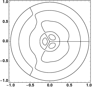
(a) $p=4$: $\hat{\psi}_{52}\approx\psi_{41}$.

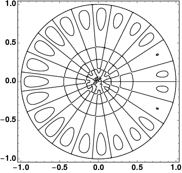
(b) $p=5$: $\hat{\psi}_{52}\approx\psi_{55}$.

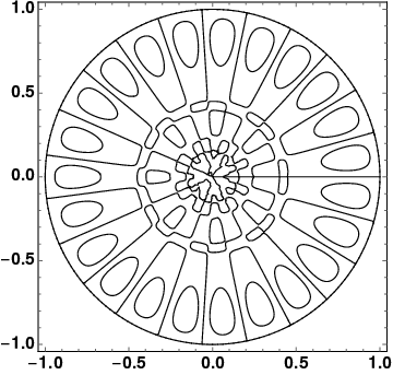
(c) $p=6$: $\hat{\psi}_{52}\approx\psi_{55}$.

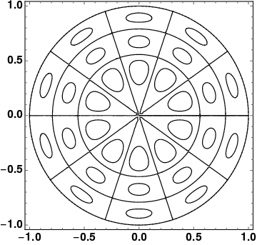
(d) $p=7$: $\hat{\psi}_{52}\approx\psi_{52}$.

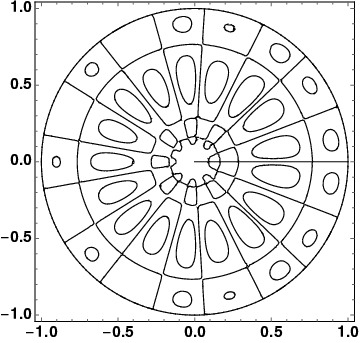
(e) $p=4$: $\hat{\psi}_{53}\approx\psi_{59}$.

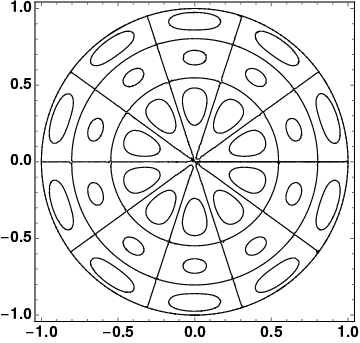
(f) $p=5$: $\hat{\psi}_{53}\approx\psi_{52}$.

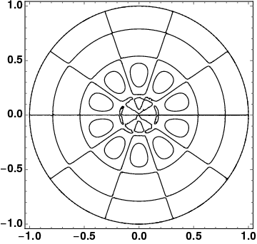
(g) $p=6$: $\hat{\psi}_{53}\approx\psi_{52}$.

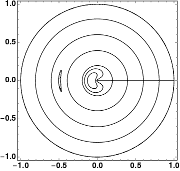
(h) $p=7$: $\hat{\psi}_{53}\approx\psi_{53}$.

Figure 1. Contour plots of computed eigenvectors $\hat{\psi}_{52}$ (top row) and $\hat{\psi}_{53}$ (bottom row) on a sequence of increasingly fine discretizations.

Example 1.1 (Slit Disk).

Let $\Omega\subset\mathbb{R}^{2}$ be the unit disk with the positive $x$-axis removed, and consider the Laplace eigenvalue problem:

$$-\Delta\psi=\lambda\psi\mbox{ in }\Omega\quad,\quad\psi=0\mbox{ on }\partial\Omega$$

The eigenvalues and vectors are known explicitly (cf. [20]), and are doubly-indexed for $m,n\in\mathbb{N}$ by

(3) $$\psi_{m,n}=J_{n/2}(j_{m,n}r)\sin(n\theta/2)\quad,\quad\lambda_{m,n}=j_{m,n}^{2}~{},$$

where $J_{n/2}$ is the first-kind Bessel function of order $n/2$ and $j_{m,n}$ is the $m$th positive root of $J_{n/2}$; $r\in[0,1]$ and $\theta\in[0,2\pi]$ are the usual polar coordinates. Since $J_{1/2}(z)=\sqrt{2/(\pi z)}\,\sin z$, we see that $\lambda_{m,1}=(m\pi)^{2}$, and $\psi_{m,1}\in H^{3/2-\epsilon}(\Omega)$ only for $\epsilon>0$.

It is well-known that, when $\nu\in\mathbb{Q}$ and $\ell\in\mathbb{N}$, then $J_{\nu}$ and $J_{\nu+\ell}$ have no common positive roots (cf [24, pp. 484-485]), and that the positive roots of Bessel functions are simple. It follows from the first of these assertions that $J_{n/2}$ and $J_{n^{\prime}/2}$ have no common positive roots when $n$ and $n^{\prime}$ have the same parity, but it does not rule out that they may have common positive roots when $n$ and $n^{\prime}$ do not have the same parity. We have not determined whether or not all eigenvalues in this example are simple, but we have verified that at least the first 100 are, which will be sufficient for our purposes. If the eigenvalues are ordered in an increasing sequence as described above, this induces a natural mapping $(m,n)\mapsto k$ from index pairs to absolute indices. For $k\leq 100$ we know that this map is invertible, with $52\mapsto(3,10)$ and $53\mapsto(5,1)$, for example. Contour plots of $\psi_{3,10}=\psi_{52}$ and $\psi_{5,1}=\psi_{53}$ are given, together with their corresponding eigenvalues, in Figure 2. This illustrates that eigenmodes associated with eigenvalues that are relatively close to each other can have very different regularities; $\psi_{53}\in H^{3/2-\epsilon}(\Omega)$ only for $\epsilon>0$, but $\psi_{52}\in H^{\ell}(\Omega)$ for all $\ell$.

(a) Eigenvector $\psi_{52}$.

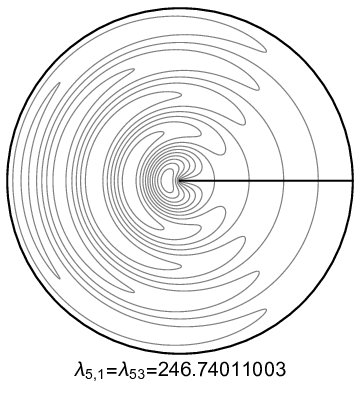
(b) Eigenvector $\psi_{53}$.

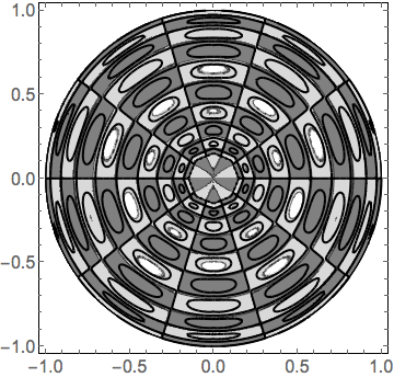
(c) Eigenvector error $e_{52}$ and approximation $\varepsilon_{52}$.

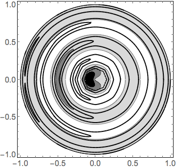
(d) Eigenvector error $e_{53}$ and approximation $\varepsilon_{53}$.

Figure 2. Two consecutive eigenvectors $\psi_{j}$ for the slit disk, together with finite element errors $e_{j}=\psi_{j}-\hat{\psi}_{j}$ and their approximations $\varepsilon_{j}\approx e_{j}$. The eigenfunction error $e_{j}$ is given as a greyscale contour plot, and thick black contour lines of its approximation $\varepsilon_{j}$ are overlaid.

We also use this example to illustrate a mixing of modes that may occur in eigenvalue/vector approximations. In Figure 1 we show contour plots of the computed eigenvectors $\hat{\psi}_{52}$ and $\hat{\psi}_{53}$ corresponding to $\hat{\lambda}_{52}$ and $\hat{\lambda}_{53}$, for a sequence of increasingly fine discretizations that will be described in Section 3. The computed eigenvectors are then identified with the true eigenvectors they most closely resemble, based on analysis of their behavior (e.g. sign changes) in both the angular and radial directions. We describe this procedure in greater detail later. We note that $\psi_{53}=\psi_{5,1}$ is approximated by $\hat{\psi}_{53}$ only on the finest of these discretizations, whereas $\psi_{52}=\psi_{3,10}$ is approximated by $\hat{\psi}_{53}$ on two of the discretizations, and only moves into its proper position on the finest discretization—compare with Figure 2. In its progression toward approximating $\psi_{52}$, $\hat{\psi}_{52}$ approximates $\psi_{41}=\psi_{4,3}$ on the coarsest of the discretizations, and $\psi_{55}=\psi_{1,23}$ on the next two discretizations. Similarly, $\hat{\psi}_{53}$ approximates $\psi_{59}=\psi_{2,17}$ on the coarsest discretization, and $\psi_{52}$ on the next two discretizations. The computed approximations $\hat{\lambda}_{52}$ and $\hat{\lambda}_{53}$ both decrease monotonically toward their respective values $\lambda_{52}$ and $\lambda_{53}$ as the discretizations are enriched, as they should, with with $\hat{\lambda}_{52}=317.923$ and $\hat{\lambda}_{53}=318.275$ on the coarsest of the discretizations ($p=4$), and $\hat{\lambda}_{52}=247.941$ and $\hat{\lambda}_{53}=250.782$ on the finest of the discretizations ($p=7$) used for Figure 1.

Having identified how fine our discretizations must be in order to properly identify $\hat{\psi}_{52}$ and $\hat{\psi}_{53}$ with $\psi_{52}$ and $\psi_{53}$, we highlight a feature of the error estimation technique that we propose. Our approach to error estimation in the eigenvalue context is based on related work for source problems [12], in that eigenvector errors are approximated as functions in an auxiliary space that, in a practical sense, complements the finite element space in which the eigenvectors are approximated. For related work in the context of low-order finite element eigenvalue/vector approximations, we refer to [11, 2]. Appropriate norms of such approximate error functions provide the basis for estimating eigenvalue and invariant subspace errors. Because we compute approximate eigenvector error functions, we can provide qualitative, as well as quantitative estimates of error. To illustrate this point, we compute approximate eigenvectors $\hat{\psi}_{52},\hat{\psi}_{53}$ in suitable finite element spaces, and provide contour plots of the errors $e_{j}=\psi_{j}-\hat{\psi}_{j}$ and approximate errors $\varepsilon_{j}\approx e_{j}$, also in Figure 2. The functions $\psi_{j}$ and $\hat{\psi}_{j}$ have been normalized so that $\|\psi_{j}\|_{0}=\|\hat{\psi}_{j}\|_{0}=1$ and $\hat{\psi}_{j}$ is a better approximation of $\psi_{j}$ than is $-\hat{\psi}_{j}$. The mesh used for these computations, shown in Figure 3, resolves these modes close to the origin with errors that are an order of magnitude smaller than those a bit farther away. Because of this, for visual clarity we have omitted the contours of $\varepsilon_{j}$ in the central portion of Figures 2(c)-(d).

The rest of the paper is organized as follows. In Section 2 we present general results concerning estimation of error that is suitable for clusters of eigenvalues and their corresponding invariant subspaces. In Section 3, we describe the $p$- and $hp$-finite element spaces that are used in this work, the technique we have used to identify computed eigenmodes with true eigenmodes when the latter are known (as was done in Example 1.1), and our approach for a posteriori error estimation in this context. We provide a detailed case study in Section 4 of examples having many clustered eigenvalues throughout the spectrum, which were constructed taking a pair of isospectral drums and connecting them in various ways with narrow bridges. We focus on 2D problems in Sections 3 and 4, but we emphasize that the theoretical development in Section 2 is not dimension-dependent.

2. Theoretical Results

It will be convenient for the development of the error estimates to express (1) in terms of operators. The bilinear form defines an operator $\mathcal{A}$ by a representation theorem of Friedrichs [5] (see also [16, Chapter 6, Theorem 2.1]), such that $(\mathcal{A}v,w)=B(v,w)$ for all $v\in\mathrm{Dom}(\mathcal{A})\subset\mathcal{H}$ and $w\in\mathcal{H}$, and we write $\mathcal{A}v=-\nabla\cdot A\nabla v+bv$. The operator $\mathcal{A}$ is self-adjoint and positive definite, and is typically viewed as an unbounded operator on $L^{2}(\Omega)$. The variational eigenvalue problem (1) is equivalent to the operator eigenvalue problem: Find $(\lambda,\psi)\in\mathbb{R}\times\mathrm{Dom}(\mathcal{A})$, $\psi\neq 0$, such that $\mathcal{A}\psi=\lambda\psi$. A second representation theorem (see [16, Chapter 6, Theorem 2.23]) expresses the bilinear form in terms of the self-adjoint and positive definite square-root of $\mathcal{A}$, $\mathcal{A}^{1/2}$ (see [16, Chapter 5, Theorem 3.35]),

$$B(v,w)=(\mathcal{A}^{1/2}v,\mathcal{A}^{1/2}w)\mbox{ for all }v,w\in\mathrm{Dom}(\mathcal{A}^{1/2})=\mathcal{H}~{},$$

and we see that $|\!|\!|v|\!|\!|=\|\mathcal{A}^{1/2}v\|_{0}$.

Let $\mathrm{Spec}(\mathcal{A})$ denote the spectrum of $\mathcal{A}$. Given a finite subset $\Lambda\subset\mathrm{Spec}(\mathcal{A})$, let

$$E(\Lambda)=\mathrm{span}\{\psi\in\mathrm{Dom}(\mathcal{A}):\,\mathcal{A}\psi=\lambda\psi\mbox{ for some }\lambda\in\Lambda\}$$

be the associated invariant subspace. Let $S(\Lambda)$ be the $L^{2}(\Omega)$-orthogonal projector onto $E(\Lambda)$. When $\Lambda=\{\lambda\}$, we use $E(\lambda)$ and $S(\lambda)$. It is well-known that $S(\Lambda)$ is also the orthogonal projector onto $E(\lambda)$ with respect to the energy inner-product. These orthogonal projection properties are stated as best approximation results in the following proposition.

Proposition 2.1.

Let $\Lambda\subset\mathrm{Spec}(\mathcal{A})$ be a finite set, $E=E(\Lambda)$ and $S=S(\Lambda)$. For any $v\in\mathcal{H}$, it holds that $\left\|(I-S)v\right\|=\inf_{w\in E}\left\|v-w\right\|$, where $\left\|\cdot\right\|$ denotes either the $L^{2}$ or energy norm. In the case of the $L^{2}$ norm, we may allow $v\in L^{2}(\Omega)$.

Taking $\Lambda$ and $S=S(\Lambda)$ as above, let $\hat{\mu}\not\in\mathrm{Spec}(\mathcal{A})\setminus\Lambda$ be a non-zero real number, and $\hat{\phi}\in\mathcal{H}$. It can be seen in the proof of [6, Proposition 2] that

(4) $$(I-S)\hat{\phi}=-[\mathcal{A}^{1/2}(\hat{\mu}-\mathcal{A}^{\prime})^{-1}(I-S)][\mathcal{A}^{1/2}(\hat{\phi}-\mathcal{A}^{-1}(\hat{\mu}\hat{\phi}))]~{}$$

where $\mathcal{A}^{\prime}=\mathcal{A}(I-S)$. It follows that

$$|\!|\!|(I-S)\hat{\phi}|\!|\!|=\|\mathcal{A}^{1/2}(I-S)\hat{\phi}\|_{0}=\|\mathcal{A}(\hat{\mu}-\mathcal{A}^{\prime})^{-1}(I-S)][\mathcal{A}^{1/2}(\hat{\phi}-\mathcal{A}^{-1}(\hat{\mu}\hat{\phi}))\|_{0}~{}.$$

Since all of the operators in (4) commute, we also have

$$\|(I-S)\hat{\phi}\|_{0}=\|\mathcal{A}(\hat{\mu}-\mathcal{A}^{\prime})^{-1}(I-S)][(\hat{\phi}-\mathcal{A}^{-1}(\hat{\mu}\hat{\phi}))\|_{0}~{}.$$

From these identities, we obtain the estimates

(5) $$\|(I-S)\hat{\phi}\|\leq C(\hat{\mu},\Lambda)\|\hat{\phi}-\mathcal{A}^{-1}(\hat{\mu}\hat{\phi})\|~{},$$

where $\left\|\cdot\right\|$ denotes either the $L^{2}$ or energy norms, and the constant $C(\hat{\mu},\Lambda)$ is given by

(6) $$C(\hat{\mu},\Lambda)=\|\mathcal{A}(\hat{\mu}-\mathcal{A}^{\prime})^{-1}(I-S)\|_{0}=\|\mathcal{A}^{\prime}(\hat{\mu}-\mathcal{A}^{\prime})^{-1}\|_{0}=\max_{\xi\in(\mathrm{Spec}{\mathcal{A}}\setminus\Lambda)\cup\{0\}}\frac{\xi}{|\xi-\hat{\mu}|}~{}.$$

The final identity can be found, for example, in [16, Chapter 5, Section 3.5], and uses the fact that $\mathrm{Spec}{\mathcal{A}^{\prime}}=(\mathrm{Spec}{\mathcal{A}}\setminus\Lambda)\cup\{0\}$. If $\Lambda=\{\lambda\}$, we use $C(\hat{\mu},\lambda)$ for this constant.

Now let $E=E(\Lambda)$, with $\dim E=r$. Suppose we are given a real subspace $\hat{E}\subset\mathcal{H}$ of dimension $r$, as well as an $r$-tuple of positive numbers $(\hat{\mu}_{1},\ldots,\hat{\mu}_{r})$ with $\hat{\mu}_{i}\not\in\mathrm{Spec}(\mathcal{A})\setminus\Lambda$, and $\hat{\mu}_{1}\leq\cdots\leq\hat{\mu}_{r}$. Taking $\{\hat{\phi}_{1},\ldots,\hat{\phi}_{r}\}$ as a basis of $\hat{E}$, we identify $\hat{\mu}_{i}$ with $\hat{\phi}_{i}$. It is natural to think of $\hat{\Lambda}=\{\hat{\mu}_{1},\ldots,\hat{\mu}_{r}\}$ and $\hat{E}$ as approximations of $\Lambda$ and $E$ obtained by an $hp$-finite element procedure, and we will do so later, but for now we work with the given level of generality. Of particular interest in our discussion is the relative error in energy norm between $\hat{v}\in\hat{E}$ and its projection $S\hat{v}\in E$. Letting $G,H\in\mathbb{R}^{r\times r}$ be the Gram matrices given by

(7) $$G_{ij}=B(\hat{\phi}_{j},\hat{\phi}_{i})\quad,\quad H_{ij}=B((I-S)\hat{\phi}_{j},(I-S)\hat{\phi}_{i})~{},$$

and $\mathbf{v}\in\mathbb{R}^{r}$ be the coefficient vector of $\hat{v}$ with respect to the (ordered) basis $(\hat{\phi}_{1},\ldots,\hat{\phi}_{r})$, we have

(8) $$\frac{|\!|\!|(I-S)\hat{v}|\!|\!|^{2}}{|\!|\!|\hat{v}|\!|\!|^{2}}=\frac{\mathbf{v}^{t}H\mathbf{v}}{\mathbf{v}^{t}G\mathbf{v}}~{}.$$

This naturally leads to our first key result.

Theorem 2.2.

We have the eigenvector error trace estimate

(9) $$\sup_{\hat{v}\in\hat{E}}\frac{|\!|\!|(I-S)\hat{v}|\!|\!|^{2}}{|\!|\!|\hat{v}|\!|\!|^{2}}\leq\frac{[C(\hat{\Lambda},\Lambda)]^{2}}{\lambda_{\min}(G)}\,\sum_{j=1}^{r}|\!|\!|\hat{\phi}_{j}-\mathcal{A}^{-1}(\hat{\mu}_{j}\hat{\phi}_{j})|\!|\!|^{2}~{},$$

where $C(\hat{\Lambda},\Lambda)=\max\{C(\hat{\mu}_{j},\Lambda):\,1\leq j\leq r\}$. If we further assume that $B(\hat{\phi}_{i},\hat{\phi}_{j})=\hat{\mu}_{i}\delta_{ij}$, then we have the following modification of (9),

(10) $$\sup_{\hat{v}\in\hat{E}}\frac{|\!|\!|(I-S)\hat{v}|\!|\!|^{2}}{|\!|\!|\hat{v}|\!|\!|^{2}}\leq[C(\hat{\Lambda},\Lambda)]^{2}\,\sum_{j=1}^{r}\frac{|\!|\!|\hat{\phi}_{j}-\mathcal{A}^{-1}(\hat{\mu}_{j}\hat{\phi}_{j})|\!|\!|^{2}}{\hat{\mu}_{j}}~{},$$

as well as the eigenvalue error trace estimate,

(11) $$\sum_{j=1}^{r}(\hat{\mu}_{j}-\mu_{j})\leq[C(\hat{\Lambda},\Lambda)]^{2}\,\sum_{j=1}^{r}|\!|\!|\hat{\phi}_{j}-\mathcal{A}^{-1}(\hat{\mu}_{j}\hat{\phi}_{j})|\!|\!|^{2}~{},$$

where $\Lambda=\{\mu_{1},\ldots,\mu_{r}\}$, with $\mu_{1}\leq\cdots\leq\mu_{r}$.

Proof.

The ratio in (8) is clearly controlled by the eigenvalues of $G^{-1}H$, and a simple upper-bound is given by $\mathrm{trace}(H)/\lambda_{\min}(G)$. Combining this with (5) and (6) yields the bound (9). Under the further assumptions on $\hat{\phi}_{j}$ and $\hat{\mu}_{j}$, $G$ is diagonal, and we instead bound (8) by $\mathrm{trace}(G^{-1}H)$ to obtain (10). For the eigenvalue estimate, let $\{\phi_{1},\ldots,\phi_{r}\}$ be an orthonormal eigenbasis of $E$, with $\mu_{j}=|\!|\!|\phi_{j}|\!|\!|^{2}$. We have

$$\sum_{i=1}^{r}|\!|\!|(I-S)\hat{\phi}_{i}|\!|\!|^{2} =\sum_{i=1}^{r}\left(|\!|\!|\hat{\phi}_{i}|\!|\!|^{2}-\sum_{j=1}^{r}\mu_{j}[(\phi_{j},\hat{\phi}_{i})]^{2}\right)$$

$$=\sum_{i=1}^{r}\hat{\mu}_{i}-\sum_{j=1}^{r}\mu_{j}\sum_{i=1}^{r}[(\phi_{j},\hat{\phi}_{i})]^{2}\geq\sum_{i=1}^{r}\hat{\mu}_{i}-\sum_{j=1}^{r}\mu_{j}~{}.$$

The bounds $|\!|\!|(I-S)\hat{\phi}_{i}|\!|\!|\leq C(\hat{\mu}_{j},\Lambda)\|\hat{\phi}_{j}-\mathcal{A}^{-1}(\hat{\mu}_{j}\hat{\phi}_{j})\|$ complete the proof. ∎

Remark 2.3.

The subspace gap (cf. [16, Chapter 4, Section 2]) is a standard measure of distance between subspaces. The “Pair of Projectors Alternative” [16, Chapter 1, Theorem 6.34], implies that, if $\sup_{\hat{v}\in\hat{E}}|\!|\!|(I-S)\hat{v}|\!|\!|/|\!|\!|\hat{v}|\!|\!|<1$, then

(12) $$\mathrm{gap}(E,\hat{E})=\sup_{\hat{v}\in\hat{E}}\inf_{v\in E}\frac{|\!|\!|v-\hat{v}|\!|\!|}{|\!|\!|\hat{v}|\!|\!|}=\sup_{v\in E}\inf_{\hat{v}\in\hat{E}}\frac{|\!|\!|v-\hat{v}|\!|\!|}{|\!|\!|v|\!|\!|}<1~{}.$$

More generally, the gap between two subspaces $M,N$ of $\mathcal{H}$, with respect to the energy norm is

$$\mathrm{gap}(M,N)=\max\left\{\sup_{w\in M}\inf_{v\in N}\frac{|\!|\!|v-w|\!|\!|}{|\!|\!|w|\!|\!|}\,,\,\sup_{v\in N}\inf_{w\in M}\frac{|\!|\!|v-w|\!|\!|}{|\!|\!|v|\!|\!|}\right\}~{}.$$

If $P_{M}$ and $P_{N}$ are the corresponding orthogonal projectors (with respect to the energy inner-product), then $\mathrm{gap}(M,N)=|\!|\!|P_{M}-P_{N}|\!|\!|$, so we see that the gap provides a metric between subspaces. In fact, when $M$ and $N$ have the same finite dimension, $\mathrm{gap}(M,N)$ is the sine of the largest principle angle between the these subspaces (cf. [17]). A natural alternative to the subspace gap is to measure the distance between the corresponding orthogonal projectors using a Hilbert-Schmidt norm. This is the approach taken in [4], for example.

Remark 2.4.

Suppose that $\Lambda,\hat{\Lambda}\subset(a,b)$ for some $0<a<b$, and $\mathrm{Spec}(A)\setminus\Lambda\subset(0,a]\cup[b,\infty)$. Then we have

(13) $$C(\hat{\Lambda},\Lambda)=\max\{C(\hat{\mu}_{1},\Lambda),C(\hat{\mu}_{r},\Lambda)\}\leq\max\left\{\frac{a}{\hat{\mu}_{1}-a},\frac{b}{b-\hat{\mu}_{r}}\right\}~{}.$$

For $f\in L^{2}(\Omega)$, we define $u(f)\in\mathcal{H}$ and $\hat{u}(f)\in V$ by

(14) $$B(u(f),v)=(f,v)_{0}\mbox{ for all }v\in\mathcal{H}\quad,\quad B(\hat{u}(f),v)=(f,v)_{0}\mbox{ for all }v\in V~{}.$$

Now suppose that $(\hat{\mu}_{j},\hat{\phi}_{j})$ is a solution of (2) for $1\leq j\leq r$. Taking $f_{j}=\hat{\mu}_{j}\hat{\phi}_{j}$, we have $u(f_{j})=\mathcal{A}^{-1}(\hat{\mu}_{j}\hat{\phi}_{j})$ and $\hat{u}(f_{j})=\hat{\phi}_{j}$, and we rephrase (10) and (11) as

(15) $$\sup_{\hat{v}\in\hat{E}}\frac{|\!|\!|(I-S)\hat{v}|\!|\!|^{2}}{|\!|\!|\hat{v}|\!|\!|^{2}} \leq[C(\hat{\Lambda},\Lambda)]^{2}\,\sum_{j=1}^{r}\frac{|\!|\!|u(f_{j})-\hat{u}(f_{j})|\!|\!|^{2}}{\hat{\mu}_{j}}~{},$$

(16) $$\sum_{j=1}^{r}(\hat{\mu}_{j}-\mu_{j}) \leq[C(\hat{\Lambda},\Lambda)]^{2}\,\sum_{j=1}^{r}|\!|\!|u(f_{j})-\hat{u}(f_{j})|\!|\!|^{2}~{}.$$

These forms of the estimates emphasize that eigenvalue and eigenspace errors are controlled by discretization errors of source problems whose data are drawn from the discrete eigenpairs, and we will return to them in our development of practical a posteriori estimates for eigenvalue and eigenspace errors in Section 3. We also note that, in this setting, $\hat{\mu}_{j}\geq\mu_{j}$.

The upper-bound on the subspace gap provided in (15), as well as its computable counterpart in (22) are theoretically convenient over-estimates, which may be pessimistic when $r$ is large. In fact, they might seem more natural as bounds on a Hilbert-Schmidt type measure of subspace error (see Remark 2.3). The recent contribution [4] takes this approach. If we had a decent computable approximation $\tilde{H}$ of the Gram matrix $H$ from (8), we could compute the eigenvalues of generalized eigenvalue problem $\tilde{H}\mathbf{x}=\tilde{\kappa}G\mathbf{x}$ directly, and not be restricted to trace-type estimates such as (9), (10) or (15). The largest of these eigenvalues would then provide an estimate of the subspace gap (12). In Section 4.2, we illustrate how the error estimates described in Section 3 enable the computation of such an approximation $\tilde{H}$ of $H$.

The following Bauer-Fike estimate (cf. [7, Theorem 7.2.2]) provides a measure of distance between the eigenvalues of $(H,G)$ and $(\tilde{H},G)$ in terms of matrix norms.

Proposition 2.5.

Let $\tilde{H}$ be a positive semi-definite approximation of the Gram matrix $H$ from (8). If $\tilde{\kappa}$ is an eigenvalue for the pair $(\tilde{H},G)$, then

$$\min_{\kappa\in\mathrm{Spec}(H,G)}|\kappa-\tilde{\kappa}|\leq\|G^{-1/2}\|_{p}^{2}\|H-\tilde{H}\|_{p}~{},$$

for any matrix $p$-norm, where $G^{-1/2}$ is the (unique) positive definite square root of $G^{-1}$.

We note that, if $G=\mathrm{diag}(\hat{\mu}_{1},\cdots,\hat{\mu}_{r})$, then $\|G^{-1/2}\|_{p}^{2}=(\min\{\hat{\mu}_{j}\})^{-1}$. It is clear that the roles of $H$ and $\tilde{H}$ can be reversed in Proposition 2.5, so we actually have a bound on the Hausdorff distance between $K=\mathrm{Spec}(H,G)$ and $\tilde{K}=\mathrm{Spec}(\tilde{H},G)$,

(17) $$\mathrm{dist}(K,\tilde{K})\doteq\max\left\{\max_{\tilde{\kappa}\in\tilde{K}}\min_{\kappa\in K}|\kappa-\tilde{\kappa}|\,,\,\max_{\kappa\in K}\min_{\tilde{\kappa}\in\tilde{K}}|\kappa-\tilde{\kappa}|\right\}\leq\|G^{-1/2}\|_{p}^{2}\|H-\tilde{H}\|_{p}~{}.$$

In Section 3, after we have properly introduced the approximate error functions $\varepsilon_{j}$, we illustrate (17) for the Slit Disk problem and the choice $\tilde{H}_{ij}=B(\varepsilon_{j},\varepsilon_{i})$, in Example 3.3.

Remark 2.6.

In [10, 11, 2], the authors develop an a posteriori eigenvalue and eigenvector error analysis based on approximation defects, which are essentially the square roots of the eigenvalues of the pair $(H,G)$.

Remark 2.7.

A natural question would be the choice of optimal $p$. Matrix $p$-norms in general do not have a monotonic relationship and the choice of $2$ norms presents an easily computable norm. More on evaluating other matrix $p$ norms can be found in [14].

3. p and hp Finite Element Discretization, A Posteriori Estimates

Let $\Omega\subset\mathbb{R}^{2}$ be a open, bounded domain, with Lipschitz boundary $\partial\Omega$, and let $\mathcal{T}=\{T\}$ be a conforming partition of $\Omega$ into convex (curvilinear) triangles and quadrilaterals, which we call a mesh or triangulation, see Figure 3. We do not impose any restriction on the number of curved edges. Any curved elements are handled using standard blending function techniques (cf. [23]). In order to reduce the level of technicality in describing the families of finite element spaces that we will consider, we state them for only in the case of polygonal domains, partitioned into triangles and quadrilaterals.

For a given element $T$ and non-negative integer $m$, we define the local polynomial space $\mathbb{Q}_{m}(T)$ as follows. If $T$ is a triangle, then $\mathbb{Q}_{m}(T)$ consists of the polynomials of total degree $\leq m$, so $\dim\mathbb{Q}_{m}(T)=(m+2)(m+1)/2$. If $T$ is a quadrilateral, then $\mathbb{Q}_{m}(T)$ consists of polynomials of degree $\leq m$ in each variable, so $\dim\mathbb{Q}_{m}(T)=(m+1)^{2}$. For a given triangulation, $\mathcal{T}$, let $\mathbf{p}:\mathcal{T}\to\mathbb{N}$ be a function that assigns a positive integer to each element $T\in\mathcal{T}$. This map is called a $p$-vector. We define the corresponding finite element space

(18) $$V=V(\mathcal{T},\mathbf{p})=\{v\in\mathcal{H}:\,v_{|_{T}}\in\mathbb{Q}_{\mathbf{p}(T)}(T)\mbox{ for all }T\in\mathcal{T}\}~{}.$$

We note that $V\subset C(\overline{\Omega})$.

Let $\mathcal{F}=\{\mathcal{T}_{\ell}\}$ be a family of nested meshes obtained from successive refinements of an initial coarse mesh, where the index $\ell\geq 0$ refers to a refinement level. Of particular interest to us in this work are eigenproblems, such as that in Example 1.1, for which it is known that certain eigenfunctions will be singular (e.g. have unbounded derivatives) at particular points in the domain. Such points are commonly referred to as singular points, and in the case of the Laplace operator, occur at points on the boundary where there are non-convex corners, and where there is a shift in the type of boundary condition (e.g. from a Dirichlet condition to a Neumann condition). We explore examples having this second type of singular points extensively in the Section 4. The asymptotic behavior of such singularities in the vicinity of singular points is well-understood (cf. [8, 9, 19]), and based on such a priori knowledge various refinement approaches have been proposed that involve a geometric grading of element sizes toward singular points that takes into account this a priori knowledge of the singularity strength [22, Section 4.5]. Beginning with a coarse mesh $\mathcal{T}_{0}$ in which the vertex graph distance between singular points (i.e., the minimal number of edges in a path connecting these points) is at least two, the mesh grading approach is implemented using element-level replacement rules employing exact geometry description as described in [13].

Given such a family of meshes, we distinguish two families of finite element spaces defined on them. We refer to the first as the $p$-method family because it uses a fixed polynomial degree for every element in the mesh. For this family, the polynomial degree $p$ is chosen and applied to each element in the $p$th mesh in the family, $\mathcal{T}_{p}\in\mathcal{F}$, i.e. $\mathbf{p}(T)=p$ for all $T\in\mathcal{T}_{p}$. We denote the finite element spaces in this family by $V_{1,p}$, and use $4\leq p\leq 12$ for our experiments. We note that the spaces are nested, $V_{1,p}\subset V_{1,p+1}$. We refer to the second family as the $hp$-family because it uses variable polynomial degrees in the mesh. For the second family, given a polynomial degree $p$, the mesh $\mathcal{T}_{p}$ is chosen as in the first family, but polynomial degrees are no longer assigned uniformly throughout the mesh. All elements touching a singular point are assigned polynomial degree $1$, the next layer of elements are assigned polynomial degree $2$, and so on, until polynomials of degree $p$ are achieved at the $p$th layer. Any elements that are greater than $p$ layers away from all singular points are also assigned polynomial degree $p$. The initial mesh and refinement scheme ensures that there is no ambiguity in how polynomial degrees are assigned to each element. The element layers are created by nested application of the same replacement rule on every element touching a singular point. At each step, only the elements touching the singular point created at the previous one are refined making the bookkeeping of the layers simple. This is illustrated in Figure 3. We denote the finite element spaces in this by $V_{2,p}$, again using $4\leq p\leq 12$ for our experiments. As before, the spaces are nested, $V_{2,p}\subset V_{2,p+1}$, and we also note that $V_{2,p}\subset V_{1,p}$.

In practice, three types of polynomial functions are distinguished on an element: vertex functions, which vanish on all vertices except one; edge functions, which vanish on all edges except one; and element functions (interior bubble functions), which vanish on all edges. On the global (mesh) level, vertex functions are supported in the patch of elements sharing that vertex, edge functions are supported in the (one or two) elements sharing an edge, and element functions are supported in a single element. There are well-established techniques for constructing hierarchical bases for $\mathbb{Q}_{p}(T)$ (cf. [22]), starting from a basis of $\mathbb{Q}_{1}(T)$ (vertex functions), augmenting it with edge functions from $\mathbb{Q}_{2}(T)$ to form a basis for $\mathbb{Q}_{2}(T)$, further augmenting this with edge and element functions from $\mathbb{Q}_{3}(T)$ to form a basis for $\mathbb{Q}_{3}(T)$, and so on. This distinction between the types of polynomial functions enables one to build elements in which the degrees of the element functions may differ from those of the edge functions, and the degree used on one edge may differ from that used on another. In fact, this is precisely what is done in the $hp$-family, $V_{2,p}$, to allow for variable $p(T)$. In particular, when $T$ and $T^{\prime}$ are adjacent elements whose assigned polynomial degrees differ by one, say $p(T)=m$ and $p(T^{\prime})=m+1$, the polynomial degree of the edge functions associated with their shared edge is taken to be $m+1$. The use of hierarchical bases, and the distinction between edge and element functions plays a prominent role in the type of a posteriori error estimates that we now discuss.

3.1. A Posteriori Estimates

As suggested in Section 2, most clearly in the eigenvalue and eigenvector error estimates (15)-(16), we see how such error estimates are built upon those for source problems. More specifically we see that an a posteriori estimate of $|\!|\!|u(f_{j})-\hat{u}(f_{j})|\!|\!|$, where the “source” $f_{j}=\hat{\mu}_{j}\hat{\phi}_{j}$ is obtained from the approximate eigenpair $(\hat{\mu}_{j},\hat{\phi}_{j})$, provides a measure of how far $\hat{\phi}_{j}$ is from a true eigenvector and how far $\hat{\mu}_{j}$ is from a true eigenvalue. The field of a posteriori error estimation for source problems, particularly for the reaction-diffusion operators we consider here, is quite mature, so we have many well-documented methods for estimating $|\!|\!|u(f_{j})-\hat{u}(f_{j})|\!|\!|$. The one we have chosen for the present work is based on the principle of hierarchical bases, that seems particularly well-suited to the $p$- and $hp$-settings. What we use is described in detail, and rigorously tested, in [12], so we provide a general overview here, and focus on how it is used in the eigenvalue/vector context.

Given $f\in L^{2}(\Omega)$, the exact and finite element solutions, $u(f)\in\mathcal{H}$ and $\hat{u}(f)\in V$, satisfy

$$B(u(f),v)=(f,v)\mbox{ for all }v\in\mathcal{H}\quad,\quad B(\hat{u}(f),v)=(f,v)\mbox{ for all }v\in V~{}.$$

We compute an approximate error function $\varepsilon(f)\in W$ in an auxiliary subspace $W\subset\mathcal{H}$ as the projection of $u(f)-\hat{u}(f)$ onto $W$,

(19) $$B(\varepsilon(f),v)=B(u(f)-\hat{u}(f),v)=(f,v)-B(\hat{u}(f),v)\mbox{ for all }v\in W~{}.$$

The error space $W$ is chosen so that $V\cap W=\{0\}$, $W$ is defined on the same mesh as $V$, and $V\oplus W$ is a richer approximation space on this mesh. We adopt the approach suggested in [12] for problems in 2D, which we describe at the level of elements. If element functions of degree $m$ are used on an element $T$ in $V$, then element functions of degree $m+2$ are used on this same element in $W$. If edge functions of degree $m$ are used on an edge $e$ in $V$, then edge functions of degree $m+1$ are used on this same edge in $W$. We slightly rephrase [12, Theorem 1.4] in our context for the energy norm. We take $\mathcal{E}$ to be the set of edges of the mesh that are not on the Dirichlet part of the boundary, and define the volumetric residual, $R_{T}=f-(-\nabla\cdot A\nabla\hat{u}(f)+b\hat{u}(f))_{|_{T}}$. When $e\in\mathcal{E}$ is an interior edge, we define the edge residual as $r_{e}=(A\nabla\hat{u}(f)\cdot\mathbf{n}_{T})_{|_{T}}+(A\nabla\hat{u}(f)\cdot\mathbf{n}_{T^{\prime}})_{|_{T}^{\prime}}$, where $T$ and $T^{\prime}$ are the cells sharing this egde, and $\mathbf{n}_{T}$ and $\mathbf{n}_{T^{\prime}}$ are their outward unit normals. For a Neumann boundary edge, we define the edge residual as $r_{e}=(A\nabla\hat{u}(f)\cdot\mathbf{n}_{T})_{|_{T}}$. With these definitions in hand, we can state the theorem.

Theorem 3.1.

There is a constant $c$, depending on the shape-regularity of $\mathcal{T}$ and the polynomial degree $p$ such that

$$|\!|\!|\varepsilon(f)|\!|\!|\leq|\!|\!|u(f)-\hat{u}(f)|\!|\!|\leq c\left(|\!|\!|\varepsilon(f)|\!|\!|+\mathrm{osc}(R,r,\mathcal{T})\right)~{},$$

where the residual oscillation is defined by

$$[\mathrm{osc}(R,r,\mathcal{T})]^{2}=\sum_{T\in\mathcal{T}}h_{T}^{2}\inf_{\kappa\in\mathbb{Q}_{p-1}(T)}\|R_{T}-\kappa\|_{L^{2}(T)}^{2}+\sum_{e\in\mathcal{E}}|e|\inf_{\kappa\in\mathbb{Q}_{p-1}(e)}\|r_{e}-\kappa\|_{L^{2}(e)}^{2}~{},$$

where $h_{T}$ and $|e|$ are the diameter of $T$ and length of the edge $e$, respectively.

The proof given in [12] was given for simplicial meshes, but its performance was rigorously tested for more general meshes containing both (curvilinear) triangles and quadrilaterals in 2D, and hexahedral meshes in 3D. Although [12] provides compelling numerical evidence that $c$ is independent of $p$, such independence has not been theoretically established.

Remark 3.2.

If $A$ is piecewise constant on $\Omega$, and constant on each $T\in\mathcal{T}$, then the residual oscillation term in Theorem 3.1 simplifies to

$$[\mathrm{osc}(R,r,\mathcal{T})]^{2}=\sum_{T\in\mathcal{T}}h_{T}^{2}\inf_{\kappa\in\mathbb{Q}_{p-1}(T)}\|b\hat{u}(f)-\kappa\|_{L^{2}(T)}^{2}~{}.$$

In our examples, $b=0$ as well. In this case, there is no residual oscillation at all, and the error estimate of Theorem 3.1 becomes

(20) $$|\!|\!|\varepsilon(f)|\!|\!|\leq|\!|\!|u(f)-\hat{u}(f)|\!|\!|\leq c|\!|\!|\varepsilon(f)|\!|\!|~{}.$$

In the eigenvalue context, suppose we have computed approximate eigenpairs $\{(\hat{\mu}_{i},\hat{\phi}_{i}):\,1\leq i\leq r\}$ in $V$, with $B(\hat{\phi}_{i},v)=\hat{\mu}_{i}(\hat{\phi}_{i},v)$ for all $v\in V$ and $(\hat{\phi}_{i},\hat{\phi}_{j})=\delta_{ij}$. Our approximation $\tilde{H}$ of the matrix $H$ in (7) is given by

(21) $$\tilde{H}_{ij}=B(\varepsilon_{j},\varepsilon_{i})\quad,\quad\varepsilon_{k}=\varepsilon(f_{k})\quad,\quad f_{k}=\hat{\mu}_{k}\hat{\phi}_{k}~{}.$$

The matrix $G$ is diagonal, $G=\mathrm{diag}(\hat{\mu}_{1},\ldots,\hat{\mu}_{r})$. Assuming piecewise constant $A$ and $b=0$, as in Remark 3.2, in order to state eigenvector and eigenvalue error estimates without residual oscillation terms, we have

(22) $$\sup_{\hat{v}\in\hat{E}}\frac{|\!|\!|(I-S)\hat{v}|\!|\!|^{2}}{|\!|\!|\hat{v}|\!|\!|^{2}} \leq c^{2}[C(\hat{\Lambda},\Lambda)]^{2}\,\sum_{j=1}^{r}\frac{|\!|\!|\varepsilon_{j}|\!|\!|^{2}}{\hat{\mu}_{j}}~{},$$

(23) $$\sum_{j=1}^{r}(\hat{\mu}_{j}-\mu_{j}) \leq c^{2}[C(\hat{\Lambda},\Lambda)]^{2}\,\sum_{j=1}^{r}|\!|\!|\varepsilon_{j}|\!|\!|^{2}~{}.$$

For convenience, the corresponding estimates for the approximation errors associated with a single ($r=1$), simple, eigenvalue $\mu_{1}=\lambda_{k}$ with eigenvector $\phi_{1}=\psi_{k}$ and the computed eigenpair $(\hat{\mu}_{1},\hat{\phi}_{1})=(\hat{\lambda}_{k},\hat{\psi}_{k})$ are

(24) $$\inf_{v\in\mathrm{span}\{\psi_{k}\}}|\!|\!|\hat{\psi}_{k}-v|\!|\!|\leq C_{k}\,|\!|\!|\varepsilon(\hat{\lambda}_{k}\hat{\psi}_{k})|\!|\!|\quad,\quad\hat{\lambda}_{k}-\lambda_{k}\leq C_{k}^{2}\,|\!|\!|\varepsilon(\hat{\lambda}_{k}\hat{\psi}_{k})|\!|\!|^{2}~{},$$

where $C_{k}=c\,C(\hat{\lambda}_{k},\lambda_{k})$.

Example 3.3.

We revisit the Slit Disk example, Example 1.1 from Section 1, computing the approximate eigenpairs $(\hat{\lambda}_{k},\hat{\psi}_{k})$, $1\leq k\leq 60$, on a sequence of $p$-version and $hp$-version finite element spaces associated with a family of meshes that are strongly graded toward the origin (see Figure 3). These meshes/spaces, which provide good approximation of features (e.g. singularities) of eigenmodes near the origin, but for smaller $p$ do not capture oscillatory behavior farther away from the origin nearly as well, were deliberately designed to demonstrate phenomena such as the mixing of modes observed in Figure 1.

(a) Mesh at 100%.

(b) Central portion of mesh at 1200%.

Figure 3. A strongly graded mesh on the Slit Disk, and a close-up.

We first consider the potential effects of this phenomena on the quality of our computable estimates of eigenvalue and eigenvector error. Our measures of “quality” are the effectivity ratios (effectivities),

(25) $$\frac{|\!|\!|\varepsilon(\hat{\lambda}_{k}\hat{\psi}_{k})|\!|\!|^{2}}{\hat{\lambda}_{k}-\lambda_{k}}\quad,\quad\frac{\|\varepsilon(\hat{\lambda}_{k}\hat{\psi}_{k})\|_{0}}{\|\psi_{k}-\hat{\psi}_{k}\|_{0}}\quad,\quad\frac{|\!|\!|\varepsilon(\hat{\lambda}_{k}\hat{\psi}_{k})|\!|\!|}{|\!|\!|\psi_{k}-\hat{\psi}_{k}|\!|\!|}~{}.$$

Although our error estimates were only established for the energy norm, we consider function error in $L^{2}$ as well. The choice of $\psi_{k}$ is normalized by taking $\|\psi_{k}\|_{0}=\|\hat{\psi}_{k}\|_{0}=1$ and $\alpha_{k}\doteq(\psi_{k},\hat{\psi}_{k})\geq 0$. We note that $S\hat{\psi}_{k}=\alpha_{k}\psi_{k}$ in this case, so $\|\psi_{k}-\hat{\psi}_{k}\|\neq\|\psi_{k}-S\hat{\psi}_{k}\|$ in either of the two norms. However, in either norm, we have $\|\psi_{k}-S\hat{\psi}_{k}\|\leq\|\psi_{k}-\hat{\psi}_{k}\|\leq\sqrt{2}\|\psi_{k}-S\hat{\psi}_{k}\|$, with equality in the upper bound achieved for the $L^{2}$-norm when $\alpha_{k}=0$, and equality approached in the lower bound (for either norm) as $\alpha_{k}$ approaches $1$. For these sequences of discretizations, $\alpha_{k}$ approached $1$ very quickly, so there were no appreciable differences between effectivities using $\|\psi_{k}-\hat{\psi}_{k}\|$ in the denominator versus using $\|\psi_{k}-S\hat{\psi}_{k}\|$. In Figure 4, we provide plots of the effectivities for both families of discretizations, and $k=1,52,53$, recalling that the computed eigenmodes $\hat{\psi}_{52}$ and $\hat{\psi}_{53}$ do not begin to meaningfully approximate $\psi_{52}$ and $\psi_{53}$, respectively, until $p=7$. The case $k=1$, for which nothing unexpected happens, is considered merely as a comparative baseline. The poor effectivities of the estimates of the eigenmode approximation errors for $k=52,53$ when $p<7$ stand out, and are not surprising, because $\hat{\psi}_{k}$ is actually approximating $\psi_{j}$ for some $j\neq k$ when $p<7$. In light of this, we also provide plots of the ratios $\|\varepsilon_{k}(\hat{\lambda}_{k}\hat{\psi}_{k})\|/\|\psi_{j}-\hat{\psi}_{k}\|$ for both norms, where $\psi_{j}$ is also normalized as described above, as well as plots of $|\!|\!|\varepsilon(\hat{\lambda}_{k}\hat{\psi}_{k})|\!|\!|^{2}/(\hat{\lambda}_{k}-\lambda_{j})$ for the eigenvalue $\lambda_{j}$ corresponding to $\psi_{j}$; these plots are given in gray in Figure 4. Complementary eigenvalue and eigenmode convergence graphs are given in Figure 5. Since the convergence histories for both the $p$ and $hp$-families were very similar, only those for the $p$-family are shown. For $p\geq 6$, we observe a “staircase” pattern to the errors, where at first it would appear that the error decreases only at odd $p$. This kind of staircase convergence phenomenon has been observed elsewhere for $p$-method approximations on large elements (cf. [1, Figures 2.4 and 2.5]). In our case, we expect that this effect is present for $k=52,53$ because the corresponding eigenmodes oscillate within the large elements away from the origin—the behavior of the eigenmodes near the origin is resolved well by the highly graded mesh. Since $\hat{\psi}_{k}$ does not approximate $\psi_{k}$ for $k=52,53$ when $p\leq 6$, the corresponding errors in Figure 5 are really only meaningful for $p\geq 7$, at which point the errors take their first significant drop and begin the odd-even staircase pattern.

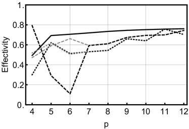
(a) $p$-version: Eigenvalue effectivity.

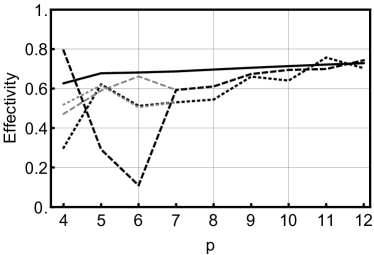
(b) $hp$-version: Eigenvalue effectivity.

(c) $p$-version: Eigenvector effectivity in $L^{2}$-norm.

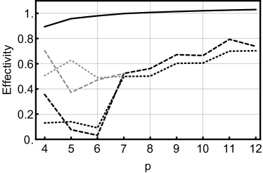
(d) $hp$-version: Eigenvector effectivity in $L^{2}$-norm.

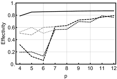
(e) $p$-version: Eigenvector effectivity in $H^{1}$-seminorm.

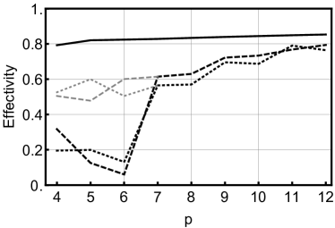
(f) $hp$-version: Eigenvector effectivity in $H^{1}$-seminorm.

Figure 4. Slit disk; Eigenvalue and eigenvector effectivity ratios for $(\lambda_{1},\psi_{1})$ (solid lines), $(\lambda_{52},\psi_{52})$ (dashed lines), $(\lambda_{53},\psi_{53})$ (dotted lines), for both the $p$- and $hp$-version. Gray curves correspond to the effectivities of the estimates when the computed eigenmode $\hat{\psi}_{k}$ is compared with the true eigenmode $\psi_{j}$ that it most closely resembles, and the computed eigenvalue $\hat{\lambda}_{k}$ is compared with the corresponding $\lambda_{j}$.

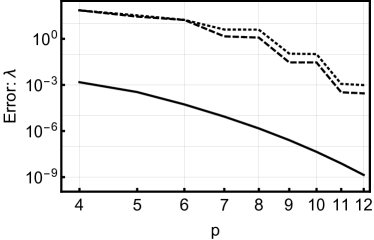
(a) Eigenvalue error.

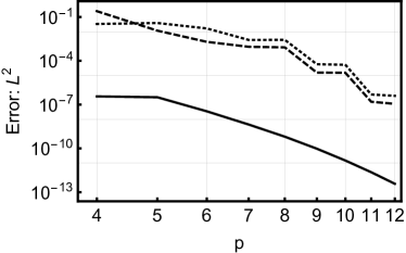
(b) Eigenvector error in squared $L^{2}$-norm.

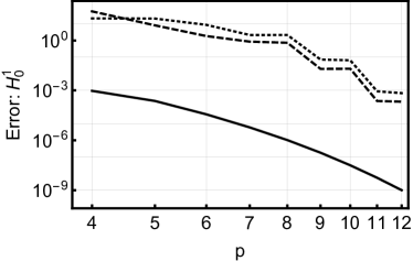
(c) Eigenvector error in squared $H^{1}$-seminorm.

Figure 5. Slit disk; Eigenvalue and eigenvector convergence for $(\lambda_{1},\psi_{1})$ (solid lines), $(\lambda_{52},\psi_{52})$ (dashed lines), $(\lambda_{53},\psi_{53})$ (dotted lines) for the $p$-version.

Before moving on to an empirical investigation of Proposition 2.5, we provide a few more remarks concerning the gray curves in Figure 4. Recalling (5), we have that $|\!|\!|\varepsilon(\hat{\lambda}_{k}\hat{\psi}_{k})|\!|\!|$ approximates $|\!|\!|\hat{\psi}_{k}-\mathcal{A}^{-1}(\hat{\lambda}_{k}\hat{\psi}_{k})|\!|\!|$ which, in turn, approximates $|\!|\!|(I-S)\hat{\psi}_{k}|\!|\!|$, where $S$ is the spectral projector for some subset of eigenvalues $\Lambda$. The theory does not force any particular choice of $\Lambda$. For example, one may choose $\Lambda=\{\lambda_{j}\}$ for some $j\neq k$. The consequences of different choices are reflected in the “constant” $C(\hat{\lambda}_{k},\Lambda)$, which will blow up as $\hat{\lambda}_{k}\to\lambda_{k}$ if $\lambda_{k}\not\in\Lambda$. Informally, we can say that $|\!|\!|\varepsilon(\hat{\lambda}_{k}\hat{\psi}_{k})|\!|\!|$ provides a reasonable estimate of the error $|\!|\!|\hat{\psi}_{k}-\psi_{j}|\!|\!|$ for some eigenmode $\psi_{j}$ (after suitable normalization), but $\psi_{j}$ might not be an eigenmode for $\lambda_{k}$ until the discretization is sufficiently rich.

Recalling the notation $K=\mathrm{Spec}(H,G)$ and $\tilde{K}=\mathrm{Spec}(\tilde{H},G)$, we now illustrate the Bauer-Fike estimate (17), using the matrix $2$-norm for the upper bound. Note that $\|G^{-1/2}\|_{2}^{2}=(\hat{\mu}_{1})^{-1}$, where $\hat{\mu}_{1}$ is the smallest approximate eigenvalue for the cluster of interest. More specifically, we will empirically compare both sides of the inequality

(26) $$\mathrm{dist}(K,\tilde{K})\leq\|H-\tilde{H}\|_{2}/\hat{\mu}_{1}~{},$$

i.e. we compare the quantities $\mathrm{dist}(K,\tilde{K})$ and $\|H-\tilde{H}\|_{2}/\hat{\mu}_{1}$. The behavior of the Hausdorff distance $\mathrm{dist}(K,\tilde{K})$ demonstrates that our computable $\tilde{H}$ provides a spectrally accurate approximation of $H$, and is therefore suitable for more nuanced estimates than those of trace-type (e.g. (15)). Comparison of the both sides of the inequality indicates that the norm bound is not a gross overestimate, and may in fact provide a relatively tight bound.

We first consider the scenario in which the cluster of interest is fixed, namely $\{\lambda_{52},\lambda_{53}\}$, and we observe the behavior of both sides of (26) as the discretization parameter $p$ is increased. In this case, $\hat{\mu}_{1}$ decreases toward $\lambda_{52}$ as $p$ increases. The results of these experiments are summarized in Figure 6.

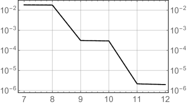
(a) $\mathrm{dist}(K,\tilde{K})$ (solid) and $\|H-\tilde{H}\|_{2}/\hat{\mu}_{1}$ (dashed); visually indistinguishable.

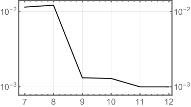
(b) Relative error $|a-b|/b$, where $a=\mathrm{dist(K,\tilde{K})}$ and $b=\|H-\tilde{H}\|_{2}/\hat{\mu}_{1}$.

Figure 6. Illustrating (26) for the Slit Disk eigenvalue cluster $\{\lambda_{52},\lambda_{53}\}$, with $7\leq p\leq 12$.

We observe the same stairstep convergence of both quantities as before, and note that $\|H-\tilde{H}\|_{2}/\hat{\mu}_{1}$ provides a very tight upper bound on $\mathrm{dist}(K,\tilde{K})$ in this case.

We next consider the scenario in which the discretization parameter $p$ is fixed, and the size of cluster is increased. More specifically, we consider two fixed discretizations, with $p=7$ and $p=12$, and investigate both sides of (26) as the cluster of interest, $\{\lambda_{1},\dots,\lambda_{r}\}$, grows with $r$, $1\leq r\leq 60$. In this case, $\hat{\mu}_{1}\approx\lambda_{1}$ is fixed as $r$ varies, so we expect the upper bound $\|H-\tilde{H}\|_{2}/\hat{\mu}_{1}$ to become more pessimistic as $r$ increases. This expectation is confirmed in Figure 7, where we nonetheless observe that both quantities exhibit very similar qualitative behavior.

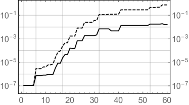
(a) Both sides of the estimate at $p=7$.

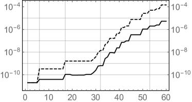
(b) Both sides of the estimate at $p=12$.

Figure 7. Illustrating (26) for the Slit Disk eigenvalue cluster $\{\lambda_{1},\ldots,\lambda_{j}\}$, $j=1,\ldots,60$, for $p=7$ (left) and $p=12$; $\mathrm{dist}(K,\tilde{K})$ (solid) and $\|H-\tilde{H}\|_{2}/\hat{\mu}_{1}$ (dashed).

Without going so far as to make a conjecture, we note the correlation between the more significant jumps in these graphs and the inclusion in the cluster of interest of the eigenfunctions having the strongest singularities, $\psi\sim r^{1/2}$ as $r\to 0$, namely $\{\psi_{1},\psi_{6},\psi_{17},\psi_{32},\psi_{53}\}$.

Remark 3.4 (Mode Detection).

The exact eigenmodes (3) have a tensor product structure. This simplifies greatly the task of identifying the closest mode $\psi_{m,n}$ to some computed $\hat{\psi}$. The indices $m$ and $n$ represent the radial and angular parts, respectively, of $\psi_{m,n}$ and thus the mode detection approach is to find $m$ and $n$ that best correspond to the computed eigenmode. For identifying the angular part $m$, $\hat{\psi}$ is evaluated along circles at two randomly chosen radii $r_{1}$ and $r_{2}$, and the wave number along these circles is computed using the discrete Fourier transform (DFT). In the unlikely case of the two values being different, a third radius is chosen for tie-breaking. We proceed similarly for the radial direction. However, in the absence of equivalent to the DFT, we project onto a set of admissible radial profiles and choose the one that is closest in the $L^{2}$ sense.

4. A Posteriori Estimates for Clusters: Numerical Experiments

In this section the focus is on a set of problems where the spectrum has a structure rich in clusters that can be identified a priori with high confidence. In this setting, it is best to estimate eigenvalue error and associated invariant subspace error over the clusters either with trace estimates such as (22)-(23) or via looking directly at $\mathrm{Spec}(\tilde{H},G)$. As a starting point, we consider a pair of complementary problems posed on half-disks, first studied by Jacobson et al.  [15], where they were shown to have identical spectra. We then consider two sets of configurations derived from the original pair by connecting these half-disks with narrow bridges, see Figure 9. This family of configurations is such that pairs of nearby eigenvalues are expected around each of the eigenvalues of the isospectral problems.

4.1. Isospectral Problems

Let $\Omega=\{(x,y):\,x^{2}+y^{2}<1\,,\,y>1\}$ be the half-disk, with boundary $\partial\Omega$ split into four parts, $\partial\Omega=\gamma_{1}\cup\gamma_{2}\cup\gamma_{3}\cup\gamma_{4}$, where

$$\gamma_{1} =\{(r\cos\theta,r\sin\theta):\;\theta=0\,,\,0\leq r\leq 1\}\cup\{(r\cos\theta,r\sin\theta):\;r=1\,,\,0\leq\theta\leq\pi/4\}~{},$$

$$\gamma_{2} =\{(r\cos\theta,r\sin\theta):\;r=1\,,\,\pi/4\leq\theta\leq 3\pi/4\}~{},$$

$$\gamma_{3} =\{(r\cos\theta,r\sin\theta):\;r=1\,,\,3\pi/4\leq\theta\leq\pi\}~{},$$

$$\gamma_{4} =\{(r\cos\theta,r\sin\theta):\;\theta=\pi\,,\,0\leq r\leq 1\}~{}.$$

The domain and boundary decomposition are shown in Figures 8a and 8b. We consider a pair of complementary problems in which we alternately apply Dirichlet and Neumann conditions on the even and odd parts of the boundary,

(27) $$-\Delta\psi=\lambda\psi\quad,\quad\psi=0\mbox{ on }\gamma_{1}\cup\gamma_{3}\quad,\quad\partial\psi/\partial n=0\mbox{ on }\gamma_{2}\cup\gamma_{4}~{},$$

(28) $$-\Delta\psi=\lambda\psi\quad,\quad\psi=0\mbox{ on }\gamma_{2}\cup\gamma_{4}\quad,\quad\partial\psi/\partial n=0\mbox{ on }\gamma_{1}\cup\gamma_{3}~{}.$$

As was proved in [15], these problems are isospectral. In other words, the eigenvalues of (27) are identical to those of (28). In Figure 8, we show a few eigenvectors associated with both problems. These were computed using refinement strategy that ensures that the lower part of the spectrum is accurately resolved. Reference values for the first fifteen eigenvalues are given in Table 1.

(a) Problem (27)

(b) Problem (28)

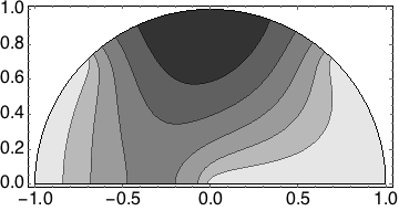
(c) $\psi_{1}$ for Problem (27)

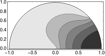
(d) $\psi_{1}$ for Problem (28)

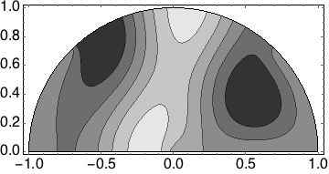
(e) $\psi_{5}$ for Problem (27)

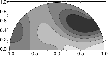
(f) $\psi_{5}$ for Problem (28)

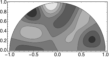
(g) $\psi_{11}$ for Problem (27)

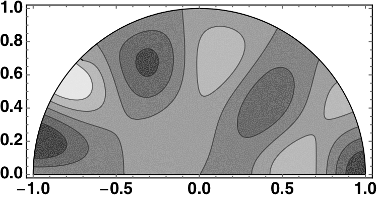
(h) $\psi_{11}$ for Problem (28)

Figure 8. Isospectral problems. The components of the boundary having Dirichlet and Neumann conditions are drawn with solid and dotted lines, respectively, in (a) and (b).

Table 1. Isospectral problems. Reference values for the lowest $15$ eigenvalues for problems (27)-(28).

$i$	$\lambda_{i}$	$i$	$\lambda_{i}$	$i$	$\lambda_{i}$
1	4.50351270364	6	4.63221446587$\times 10^{1}$	11	8.34387148427$\times 10^{1}$
2	1.35208410401$\times 10^{1}$	7	5.13074786442$\times 10^{1}$	12	9.11669451784$\times 10^{1}$
3	1.98639263212$\times 10^{1}$	8	6.24572729970$\times 10^{1}$	13	1.04631385585$\times 10^{2}$
4	3.04933490983$\times 10^{1}$	9	6.74067396593$\times 10^{1}$	14	1.09930498884$\times 10^{2}$
5	3.51893179474$\times 10^{1}$	10	7.87626319950$\times 10^{1}$	15	1.11846648035$\times 10^{2}$

4.2. Bridge Configurations

By joining two of the isospectral drums above with a narrow bridge, we can create a family of configurations in which there are clusters of eigenvalues throughout the spectrum near predictable numbers, i.e. near the eigenvalues of the isospectral domains. We take the domain to be two half-disks of raduis $1$ connected by a $1/10\times 1/4$ rectangular bridge, see Figure 9a. In this figure, we have labeled segments of the boundary A-L, and we obtain different configurations by assigning either homogeneous Dirichlet or Neumann conditions to these edges. Taking both sides of the bridge to have the same type of boundary condition, either both Dirichlet or both Neumann, there are 20 such configurations that are associated with the isospectral pair from Section 4.1, 10 having the Dirichlet bridge and 10 having the Neumann bridge. These are tabulated in Table 2, and two such configurations are shown in Figures 9c and 9d. For each eigenvalue of (27)-(28), we expect to have a pair of eigenvalues on the Bridge domain that are close to it, regardless of which of the 20 configurations of boundary conditions that we use. This is illustrated in Table 3, where we give reference values for the first 12 eigenvalues of the configurations pictured in Figure 9, together with the first 6 eigenvalues of the isospectral domains for comparison. Contour plots of the ninth and tenth eigenvectors for both of these configurations are given in Figure 10. As above, we employ refinement strategies for our experiments that ensure that the lower part of the spectrum is accurately resolved and the observed phenomena are not simply artifacts of the discretization, see Figure 9b.

(a) Bridge domain with labeled segments.

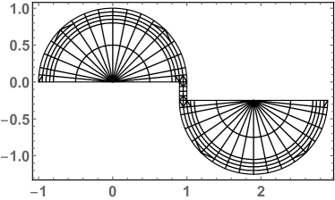
(b) $p$-type mesh used in experiments.

(c) Dirichlet bridge, Case 2.

(d) Neumann bridge, Case 9.

Figure 9. Bridge domain, a computational mesh and two configurations.

Case	A	B	C	D	E	F	G	H	I	J	K	L
1	D	X	D	N	D	D	N	X	D	N	D	N
2	D	X	D	N	D	N	D	X	D	N	D	N
3	D	X	N	D	N	N	D	X	D	N	D	N
4	D	X	N	D	N	D	N	X	D	N	D	N
5	N	X	D	N	D	D	N	X	N	D	N	D
6	N	X	N	D	N	N	D	X	N	D	N	D
7	N	X	N	D	N	D	N	X	N	D	N	D
8	N	X	D	N	D	D	N	X	D	N	D	D
9	N	X	N	D	N	N	D	X	D	N	D	D
10	D	X	N	D	N	N	D	X	N	D	N	N

Table 2. Bridge domain configurations. Edges marked D correspond to Dirichlet conditions, and those marked $N$ correspond to Neumann conditions. The Dirichlet bridge configurations correspond to X$=$D, and the Dirichlet bridge configurations correspond to X$=$N

Isospectral		Dirchlet Case 2		Neumann Case 9
$i$	$\lambda_{i}$	$i$	$\lambda_{i}$	$i$	$\lambda_{i}$
1	4.50351270364	1	4.50348976806	1	4.50318419853
		2	4.50348977820	2	4.50836662912
2	13.5208410401	3	13.5207888798	3	13.4263953994
		4	13.5207889083	4	13.5657193361
3	19.8639263212	5	19.8636968115	5	19.5509676421
		6	19.8636969659	6	19.8768798947
4	30.4933490983	7	30.4931397957	7	30.2012278561
		8	30.4931399453	8	30.5972353211
5	35.1893179474	9	35.1878233714	9	35.0596433246
		10	35.1878245124	10	35.2057946583
6	46.3221446587	11	46.3208464060	11	45.7623966583
		12	46.3208474584	12	46.4364126764

Table 3. The lowest 12 eigenvalues for two of the Bridge domain configurations compared with the lowest 6 eigenvalues for the isospectral domains.

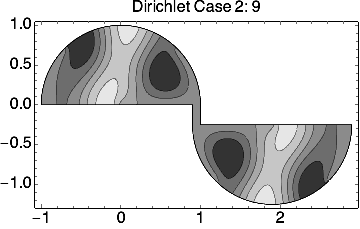
(a) $\lambda_{9}=35.1878233714$.

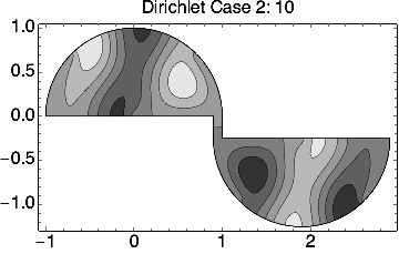
(b) $\lambda_{10}=35.1878245124$.

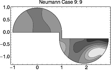
(c) $\lambda_{9}=35.0596433246$.

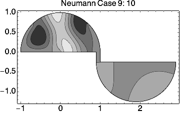
(d) $\lambda_{10}=35.2057946583$.

Figure 10. Contour plots of $\psi_{9}$ and $\psi_{10}$ for Case 2 of the Dirichlet bridge (top), and Case 9 of the Neumann Bridge (bottom). Compare with Figures 8e and 8f. Reference eigenvalues are given with each plot.

For our first set of experiments with these two configurations, we consider the Hausdorff distance, $\mathrm{dist}(\Lambda,\hat{\Lambda})$, between the reference eigenvalues $\Lambda=\{\lambda_{1},\ldots,\lambda_{r}\}$ and the computed eigenvalues $\hat{\Lambda}=\{\hat{\lambda}_{1},\ldots,\hat{\lambda}_{r}\}$ over a range of discretizations, for different values of $1\leq r\leq 12$. More specifically, we compare this Hausdorff distance with our a posteriori error estimate of it,

(29) $$\mathrm{dist}(\Lambda,\hat{\Lambda})\doteq\max\left\{\max_{\lambda\in\Lambda}\min_{\hat{\lambda}\in\hat{\Lambda}}|\lambda-\hat{\lambda}|\,,\,\max_{\hat{\lambda}\in\hat{\Lambda}}\min_{\lambda\in\Lambda}|\lambda-\hat{\lambda}|\right\}\approx\lambda_{\max}(\tilde{H})~{},$$

where $\tilde{H}\in\mathbb{R}^{r\times r}$ is given in (21). This choice of estimate is motivated as follows. Let $\lambda_{i}\in\Lambda$ and $\hat{\lambda}_{j}\in\hat{\Lambda}$ be such that $\mathrm{dist}(\Lambda,\hat{\Lambda})=|\lambda_{i}-\hat{\lambda}_{j}|$, and let $\hat{\psi}_{j}\in V$ be the discrete eigenvector associated with $\hat{\lambda}_{j}$; as usual, we assume $(\hat{\psi}_{k},\hat{\psi}_{\ell})=\delta_{k\ell}$ for $1\leq k,\ell\leq r$. Let $S$ be the orthogonal projector onto $E(\lambda_{i})$. We have the well-known identity

$$|\!|\!|(I-S)\hat{\psi}_{j}|\!|\!|^{2}-\lambda_{i}\|(I-S)\hat{\psi}_{j}\|_{0}^{2}=\hat{\lambda}_{j}-\lambda_{i}~{}.$$

If $\hat{\lambda}_{j}\geq\lambda_{i}$, which is certainly the case if $j\geq i$, then $\mathrm{dist}(\Lambda,\hat{\Lambda})\leq|\!|\!|(I-S)\hat{\psi}_{j}|\!|\!|^{2}$. Note that if the method is converging, then, asymptotically, we expect $i=j$. In any case, we have $\mathrm{dist}(\Lambda,\hat{\Lambda})\leq C|\!|\!|(I-S)\hat{\psi}_{j}|\!|\!|^{2}$. Now,

$$|\!|\!|(I-S)\hat{\psi}_{j}|\!|\!|^{2}\leq\max_{\begin{subarray}{c}v\in\hat{E}\\ \|v\|_{0}=1\end{subarray}}|\!|\!|(I-S)v|\!|\!|^{2}=\max_{\begin{subarray}{c}\mathbf{v}\in\mathbb{R}^{r}\\ \mathbf{v}^{t}\mathbf{v}=1\end{subarray}}\mathbf{v}^{t}H\mathbf{v}=\lambda_{\max}(H)~{}.$$

Here, we have identified $v\in\hat{E}$ with its coefficient vector $\mathbf{v}\in\mathbb{R}^{r}$ with respect to the discrete eigenbasis of $\hat{E}$. Finally, $\lambda_{\max}(H)$ is estimated by $\lambda_{\max}(\tilde{H})$. We highlight the difference between this sort of estimate and the trace-type estimate (23),

(30) $$\sum_{j=1}^{r}(\hat{\lambda}_{j}-\lambda_{j})\approx\mathrm{trace}(\tilde{H})~{}.$$

Note that, for the trace-type estimate, we only need computable approximations of the diagonal entries of $H$, and these may be obtained using any number of a posteriori techniques for source problems. We have opted for the auxiliary subspace approach discussed in Section 3.1, because it also naturally provides approximations of the off-diagonal entries of $H$, thereby permitting estimates of the form (29). Using the reference eigenvalues computed in a rich finite element space ($p=16$), the errors and error estimates and error estimates for $2\leq p\leq 12$ and some choices of $r$ are given in Figure 11. Computations were done for $2\leq r\leq 12$, and the plots shown in Figure 11 are representative. The effectivities of the error estimate, over all values $2\leq p,r\leq 12$, ranged between 0.574 and 2.469 for Dirichlet Case 2, and between 0.289 and 3.671 for Neumann Case 9.

(a) Dirichlet bridge, Case 2; $r=2$.

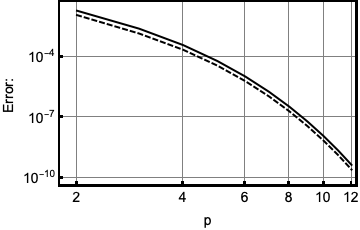
(b) Neumann bridge, Case 9; $r=2$.

(c) Dirichlet bridge, Case 2; $r=7$.

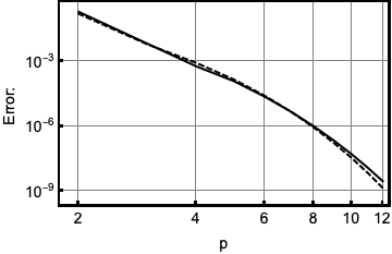
(d) Neumann bridge, Case 9; $r=7$.

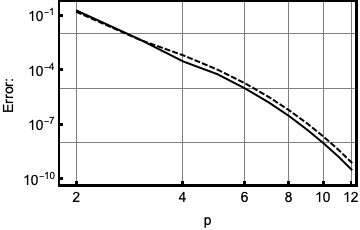
(e) Dirichlet bridge, Case 2; $r=8$.

(f) Neumann bridge, Case 9; $r=8$.

(g) Dirichlet bridge, Case 2; $r=12$.

(h) Neumann bridge, Case 9; $r=12$.

Figure 11. Eigenvalue errors $\mathrm{dist}(\Lambda,\hat{\Lambda})$ (solid) and error estimates $\lambda_{\max}(\tilde{H})$ (dashed) for two Bridge domain configurations, $\Lambda=\{\lambda_{1},\ldots,\lambda_{r}\}$.

Letting $E=\mathrm{span}\{\psi_{1},\ldots,\psi_{r}\}$ be the eigenspace of interest (computed using $p=16$), and $\hat{E}=\mathrm{span}\{\hat{\psi}_{1},\ldots,\hat{\psi}_{r}\}$ be computed approximations for various discretization parameters $2\leq p\leq 12$, we consider the subspace gap (cf. Remark 2.3 and (12)) and our computable estimate of it,

(31) $$\mathrm{gap}(E,\hat{E})=\sqrt{\lambda_{\max}(G^{-1}H)}\approx\sqrt{\lambda_{\max}(G^{-1}\tilde{H})}~{},$$

where the first equality holds provided $\lambda_{\max}(G^{-1}H)<1$, as is the case for all of our computations. Here, we take $S$ to be the orthogonal projector onto $E$ in the definition of $H$. The complementary plots to Figure 11 for convergence in subspace gap is given in Figure 12. As before, the computable estimates faithfully reflect the actual subspace gaps, with effectivities ranging between 0.747 and 0.879 for Dirichlet Case 2, and between 0.527 and 0.874 for Neumann Case 9. For comparison, we have also included the trace-type estimate $\sqrt{\mathrm{trace}(G^{-1}\tilde{H})}$ indicated in (22) in Figure 12. For this estimate, the effectivities ranged between 1.071 and 2.058 for Dirichlet Case 2, and between 1.001 and 2.052 for Neumann Case 9.

(a) Dirichlet bridge, Case 2; $r=2$.

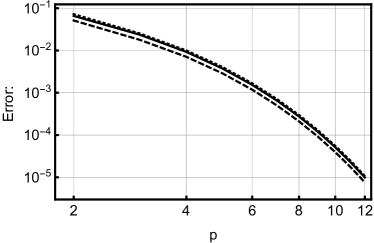
(b) Neumann bridge, Case 9; $r=2$.

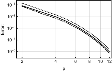
(c) Dirichlet bridge, Case 2; $r=7$.

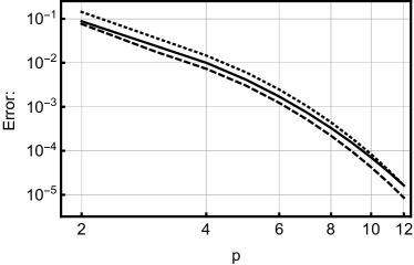
(d) Neumann bridge, Case 9; $r=7$.

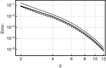
(e) Dirichlet bridge, Case 2; $r=8$.

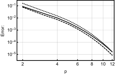
(f) Neumann bridge, Case 9; $r=8$.

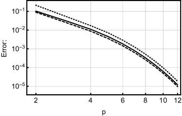
(g) Dirichlet bridge, Case 2; $r=12$.

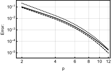
(h) Neumann bridge, Case 9; $r=12$.

Figure 12. Subspace gaps $\mathrm{gap}(E,\hat{E})$ (solid) and estimates $\sqrt{\lambda_{\max}(G^{-1}\tilde{H})}$ (dashed) and $\sqrt{\mathrm{trace}(G^{-1}\tilde{H})}$ (dotted) for two Bridge domain configurations, $E=\mathrm{span}\{\psi_{1},\ldots,\psi_{r}\}$.

Remark 4.1.

The estimates in (29) and  (31) employ the heuristics $\lambda_{\max}(\tilde{H})\approx\lambda_{\max}(H)$ and $\lambda_{\max}(G^{-1}\tilde{H})\approx\lambda_{\max}(G^{-1}H)$. At present, we only have emprical evidence that the computable quantities, i.e. those involving $\tilde{H}$, really do approximate their typically uncomputable counterparts well.

5. Conclusions

We have presented computable a posteriori estimates of the subspace gap between computed and target eigenspaces of the same size, as well for two measures of error between the corresponding computed and target eigenvalues—namely, the typical sum of eigenvalue errors and the Hausdorff distance between the computed and target eigenvalues. More rigorous theoretical footing is provided for the trace-type estimates of the subspace gap (22) and sum of eigenvalue errors (23), whereas the estimate of the Hausdorff distance between the computed and target eigenvalues (29) and the alternate estimate of the subspace gap (31) is based on the heuristic that the eigenvalues of $H$ and $\tilde{H}$ are close, for which we currently have only empirical support. These estimates have been tested extensively on a collection of problems that include both natural clusters of eigenvalues and singularities in many eigenfunctions.

References

- [1] I. Babuška and M. Suri. On locking and robustness in the finite element method. SIAM J. Numer. Anal., 29(5):1261–1293, 1992.
- [2] R. E. Bank, L. Grubišić, and J. S. Ovall. A framework for robust eigenvalue and eigenvector error estimation and ritz value convergence enhancement. Applied Numerical Mathematics, 66(0):1 – 29, 2013.
- [3] D. Boffi, D. Gallistl, F. Gardini, and L. Gastaldi. Optimal convergence of adaptive FEM for eigenvalue clusters in mixed form. Math. Comp., 86(307):2213–2237, 2017.
- [4] E. Cancés, G. Dusson, Y. Maday, B. Stamm, and M. Vohralík. Guaranteed a posteriori bounds for eigenvalues and eigenvectors: Multiplicities and clusters. Mathematics of Computation, 2020. Published electronically, July 30, 2020.
- [5] K. Friedrichs. Spektraltheorie halbbeschränkter Operatoren und Anwendung auf die Spektralzerlegung von Differentialoperatoren. Math. Ann., 109(1):465–487, 1934.
- [6] S. Giani, L. Grubišić, A. Międlar, and J. S. Ovall. Robust error estimates for approximations of non-self-adjoint eigenvalue problems. Numer. Math., 133(3):471–495, 2016.
- [7] G. H. Golub and C. F. Van Loan. Matrix computations. Johns Hopkins Studies in the Mathematical Sciences. Johns Hopkins University Press, Baltimore, MD, fourth edition, 2013.
- [8] P. Grisvard. Elliptic problems in nonsmooth domains, volume 24 of Monographs and Studies in Mathematics. Pitman (Advanced Publishing Program), Boston, MA, 1985.
- [9] P. Grisvard. Singularities in boundary value problems, volume 22 of Recherches en Mathématiques Appliquées [Research in Applied Mathematics]. Masson, Paris, 1992.
- [10] L. Grubišić. A posteriori estimates for eigenvalue/vector approximations. PAMM, 6(1):59–62, 2006.
- [11] L. Grubišić and J. S. Ovall. On estimators for eigenvalue/eigenvector approximations. Math. Comp., 78:739–770, 2009.
- [12] H. Hakula, M. Neilan, and J. S. Ovall. A posteriori estimates using auxiliary subspace techniques. J. Sci. Comput., 72(1):97–127, 2017.
- [13] H. Hakula and T. Tuominen. Mathematica implementation of the high order finite element method applied to eigenproblems. Computing, 95(1):277–301, 2013.
- [14] N. J. Higham. Estimating the matrix -norm. Numer. Math., 62(4):539–555, 1992.
- [15] D. Jakobson, M. Levitin, N. Nadirashvili, and I. Polterovich. Spectral problems with mixed dirichlet–neumann boundary conditions: Isospectrality and beyond. Journal of Computational and Applied Mathematics, 194(1):141 – 155, 2006. Special Issue: 60th birthday of Prof. Brian Davies.
- [16] T. Kato. Perturbation theory for linear operators. Classics in Mathematics. Springer-Verlag, Berlin, 1995. Reprint of the 1980 edition.
- [17] A. Knyazev, A. Jujunashvili, and M. Argentati. Angles between infinite dimensional subspaces with applications to the Rayleigh-Ritz and alternating projectors methods. J. Funct. Anal., 259(6):1323–1345, 2010.
- [18] A. V. Knyazev and M. E. Argentati. Rayleigh-Ritz majorization error bounds with applications to FEM. SIAM J. Matrix Anal. Appl., 31(3):1521–1537, 2009.
- [19] V. A. Kozlov, V. G. Maz′ya, and J. Rossmann. Elliptic boundary value problems in domains with point singularities, volume 52 of Mathematical Surveys and Monographs. American Mathematical Society, Providence, RI, 1997.
- [20] J. R. Kuttler and V. G. Sigillito. Eigenvalues of the Laplacian in two dimensions. SIAM Rev., 26(2):163–193, 1984.
- [21] E. Ovtchinnikov. Cluster robust error estimates for the Rayleigh-Ritz approximation. II. Estimates for eigenvalues. Linear Algebra Appl., 415(1):188–209, 2006.
- [22] C. Schwab. - and -Finite Element Methods. Oxford University Press, 1998.
- [23] B. Szabo and I. Babuska. Finite Element Analysis. Wiley, 1991.
- [24] G. N. Watson. A treatise on the theory of Bessel functions. Cambridge Mathematical Library. Cambridge University Press, Cambridge, 1995. Reprint of the second (1944) edition.
- [25] N. M. Wigley. Asymptotic expansions at a corner of solutions of mixed boundary value problems. J. Math. Mech., 13:549–576, 1964.