Conservative discontinuous Galerkin scheme of a gyro-averaged Dougherty collision operator

Abstract

A conservative discontinuous Galerkin scheme for a nonlinear Dougherty collision operator in full-$f$ long-wavelength gyrokinetics is presented. Analytically this model operator has the advective-diffusive form of Fokker-Planck operators, it has a non-decreasing entropy functional, and conserves particles, momentum and energy. Discretely these conservative properties are maintained exactly as well, independent of numerical resolution. In this work the phase space discretization is performed using a novel version of the discontinuous Galerkin scheme, carefully constructed using concepts of weak equality and recovery. Discrete time advancement is carried out with an explicit time-stepping algorithm, whose stability limits we explore. The formulation and implementation within the long-wavelength gyrokinetic solver of Gkeyll are validated with relaxation tests, collisional Landau-damping benchmarks and the study of 5D gyrokinetic turbulence on helical, open field lines.

1 Introduction

Many phenomena in plasma physics require kinetic treatment, meaning one must solve for the time-evolution of the particle distribution function in position-velocity phase space. For example, in collisionless astrophysical shocks the electrons and ions do not thermalize with each other nor with themselves via collisions on the time-scales of interest. Such systems are best modeled by the Vlasov-Fokker-Planck (Vlasov-FPO) equation for the particle probability distribution $f_{s}(t,\mbox{\boldmath$x$},\vv)$:

$$\frac{\partial f_{s}}{\partial t}+\nabla\cdot\left(\vv f_{s}\right)+\nabla_{\vv}\cdot\left(\mbox{\boldmath$a$}_{s}f_{s}\right)=\left(\frac{\partial f_{s}}{\partial t}\right)_{c},$$ (1)

where $\mbox{\boldmath$a$}_{s}=\left(q_{s}/m_{s}\right)\left(\mbox{\boldmath$E$}+\vv\times\mbox{\boldmath$B$}\right)$ is the acceleration due to the Lorentz force, and $q_{s}$ and $m_{s}$ the charge and mass of species $s$, respectively. One must simultaneously solve Maxwell’s equations to obtain the fields $E$ and $B$. For most plasmas of interest, the cumulative effect of frequent small-angle collisions dominates over that of rare ballistic, “large-angle” collisions, which are more common in neutral gases or fluids. Then the effect of binary encounters can be modeled by the Fokker-Planck operator (FPO), which in Rosenbluth form [1] is

$$\left(\frac{\partial f_{s}}{\partial t}\right)_{c}=-\frac{\partial}{\partial v_{i}}\left<\Delta v_{i}\right>_{s}f_{s}+\frac{1}{2}\frac{\partial^{2}}{\partial v_{i}\partial v_{j}}\left<\Delta v_{i}\Delta v_{j}\right>_{s}f_{s}.$$ (2)

Here $\left<\Delta v_{i}\right>_{s}$ indicates the average increments per unit time of the $i$-th component of the velocity of species $s$. Computation of such increments involves integrals of the distribution functions, indicating that (2) is a nonlinear integro-differential operator.

(1)-(2) and the accompanying Maxwell equations pose a formidable six-dimensional problem spanning a wide range of spatial and temporal scales, which is often numerically intractable. For magnetized environments and phenomena that evolve on a timescale much slower than the rapid particle gyration around the magnetic field, one can use a gyrokinetic reduction to five dimensions by systematically averaging over the fast gyromotion [2, 3, 4]. Additionally, in direct numerical simulations, the gyrokinetic equation permits the use of a larger time-step and coarser grids than the six-dimensional Vlasov-FPO equation. This formulation results in a change of variables from the phase-space variables ($\mbox{\boldmath$x$},\mbox{\boldmath$v$}$) to the gyro-averaged particle position, or gyrocenter, phase-space variables $(\mbox{\boldmath$R$},v_{\parallel},\mu)$, where $R$ is the gyrocenter coordinate, $v_{\parallel}$ is the velocity component parallel to the background magnetic field, and $\mu=m_{s}v_{\perp}^{2}/2B$ is the magnetic moment. Here we focus on the electrostatic gyrokinetic model evolving the gyrocenter distribution function $f_{s}(t,\mbox{\boldmath$R$},v_{\parallel},\mu)$, though the collision operator formulation and implementation presented here can also be incorporated in electromagnetic gyrokinetics [5]. The gyrokinetic equation in this case refers to

$$\frac{\partial\mathcal{J}f_{s}}{\partial t}+\nabla\cdot(\mathcal{J}f_{s}\dot{\mbox{\boldmath$R$}})+\frac{\partial}{\partial v_{\parallel}}(\mathcal{J}f_{s}\dot{v_{\parallel}})=\mathcal{J}\mathcal{C}[f_{s}],$$ (3)

where $\mathcal{J}=B_{\parallel}^{*}$ is the gyrokinetic phase-space Jacobian and $B_{\parallel}^{*}=\mbox{\boldmath$b$}\cdot\mbox{\boldmath$B$}^{*}$ is the parallel component of the effective magnetic field $\mbox{\boldmath$B$}^{*}=\mbox{\boldmath$B$}+(m_{s}v_{\parallel}/q_{s})\nabla\times\mbox{\boldmath$b$}$, where $\mbox{\boldmath$B$}=B\thinspace\mbox{\boldmath$b$}$ is the background magnetic field. We will approximate $\mbox{\boldmath$b$}\cdot\nabla\times\mbox{\boldmath$b$}\approx 0$ so that $B_{\parallel}^{*}\approx B$. The gyrokinetic nonlinear FPO is represented by $\mathcal{C}[f_{s}]$. The phase-space advection velocities $\dot{\mbox{\boldmath$R$}}=\{\mbox{\boldmath$R$},H\}$ and $\dot{v}_{\parallel}=\{v_{\parallel},H\}$ are defined in terms of the Poisson bracket

$$\{F,G\}=\frac{\mbox{\boldmath$B$}^{*}}{m_{s}B_{\parallel}^{*}}\cdot\left(\nabla F\frac{\partial F}{\partial v_{\parallel}}-\frac{\partial F}{\partial v_{\parallel}}\nabla G\right)-\frac{1}{q_{s}B_{\parallel}^{*}}\mbox{\boldmath$b$}\cdot\nabla F\times\nabla G,$$ (4)

where the Hamiltonian

$$H_{s}=\frac{1}{2}m_{s}v_{\parallel}^{2}+\mu B+q_{s}\phi$$ (5)

depends on the electrostatic potential $\phi$. To complete the electrostatic gyrokinetic system, one may solve for the electrostatic potential using the gyroaveraged Poisson equation

$$-\nabla\cdot\left(\frac{n_{i}^{g}q_{i}^{2}\rho_{s}^{2}}{T_{e}}\nabla_{\perp}\phi\right)=\sigma_{g}=q_{i}n_{i}^{g}(\mbox{\boldmath$R$},t)-en_{e}(\mbox{\boldmath$R$},t),$$ (6)

where $n_{i}^{g}$ is the ion gyro-center density, $T_{e}$ is the electron temperature and $\rho_{s}=c_{s}/\Omega_{i}$ is the ion sound gyro-radius, with $c_{s}$ being the sound speed and $\Omega_{i}$ the ion gyro-frequency. In this work we limit ourselves to the long-wavelength limit of gyrokinetics, also known as drift-kinetics. Therefore, the true potential $\phi$ appears in (5) instead of the gyroaveraged quantity $\left<\phi\right>_{\alpha}$, we use a simple form of the Poisson equation, and we neglect finite Larmor radius (FLR) effects other than the first-order polarization charge density on the left hand side of (6). The Poisson equation is also solved using a spatially constant polarization coefficient.

Several non-turbulence codes have used the full nonlinear FPO [6, 7, 8, 9], and the XGC particle-in-cell code is one of the few turbulence modeling applications employing such an operator [10]. The nonlinear FPO is less frequently found among turbulence solvers, and in continuum gyrokinetic turbulence many of the collision operators have been linear. These linear operators were developed for $\delta f$ studies [11, 12, 13] and preserved key properties of the FPO, like conservation (of particles, momentum and energy) and non-decreasing entropy. More recently, improved collision models for gyrokinetics have been formulated and implemented in several codes [14, 15, 16]. They retained important physics, such as velocity-dependent collisionalities and FLR effects, but are still linearized operators. With the exception of a few reports [15, 17], there are few simplified collision models in full-$f$ gyrokinetic turbulence modeling. Although the exact linearized gyrokinetic FPO has been formulated [18, 19], and implemented [20], and the nonlinear one formulated [21], their cost can be prohibitive for some applications. There is thus a strong interest in developing simple models that capture some of the important physics, yet can be efficiently implemented in numerical simulation.

We present here the discontinous Galerkin (DG) implementation of a nonlinear full-$f$ continuum gyroaveraged model collision operator. We build upon the formulation and implementation of similar algorithms for a Vlasov-Maxwell model operator presented in [22] (overview of DG schemes and background on various FPO solvers also appears therein), and employ the same concepts of weak equivalence, boundary correction and recovery. These algorithms are implemented in the DG gyrokinetic model within the Gkeyll computational plasma physics framework [23, 24]; download instructions as well as directions for running input files associated with this work can be found in A. In section 2, we present the Dougherty collision operator and its properties in continuous, infinite-velocity space. These features motivate the formulation of the discrete operator and its implementation, presented in section 3. In section 4, we discuss a suitable time-stepping algorithm and some of the challenges associated with the explicit finite-time integration of the collisional gyrokinetic equation. Finally, section 5 presents a number of relaxation tests showing the accuracy of the time evolution and the steady state solution with this operator, as well as a collisional Landau damping benchmark, and a complex, five-dimensional gyrokinetic simulation of open helical field-line turbulence. Additional discussion and concluding remarks are found in section 6.

2 The continuous gyroaveraged Dougherty operator

The full FPO in 2 can be simplified considerably while keeping its advective-diffusive structure. One choice is to take $\left<\Delta v_{i}\right>_{s}=-\nu_{ss}\left(v_{i}-u_{s,i}\right)$, that is, the frictional velocity change of a particle colliding with frequency $\nu_{ss}$ in a fluid of mean velocity $u_{s,i}$. The operator is simplified further by assuming that the Debye length is much smaller than the Larmor radius of a thermal particle, making perturbations within a Debye sphere isotropic. In this case one can show $\left<\Delta v_{i}\Delta v_{j}\right>_{s}\to 2\nu_{ss}v_{ts}^{2}\delta_{ij}$, where $v_{ts}^{2}=T_{s}/m_{s}$ [25]. In this work we limit ourselves to collisions between particles of the same species, and we make the additional simplification that the collision frequency is velocity-independent. In reality $\nu$ should decrease as $v^{-3}$ such that the high energy tail of the distribution is increasingly collisionless. Multi-species collisions and velocity-dependent $\nu_{ss}$ will be described in subsequent work.

For the long-wavelength gyrokinetic model in (3)-(6), the collision operator is further simplified since $\mbox{\boldmath$u$}_{s}=u_{\parallel s}\mbox{\boldmath$b$}$. Thus, the gyroaveraged Dougherty operator (GkLBO) becomes

$$\mathcal{J}\mathcal{C}[f_{s}]\equiv\nu_{ss}\left\{\frac{\partial}{\partial v_{\parallel}}\left[(v_{\parallel}-u_{\parallel s})\mathcal{J}f_{s}+v_{ts}^{2}\frac{\partial\mathcal{J}f_{s}}{\partial v_{\parallel}}\right]+\frac{\partial}{\partial\mu}\left[2\mu\mathcal{J}f_{s}+2\frac{m_{s}v_{ts}^{2}}{B}\mu\frac{\partial\mathcal{J}f_{s}}{\partial\mu}\right]\right\}.$$ (7)

The Jacobian $\mathcal{J}=B$ only varies in configuration-space and can be incorporated into the collision operator. The operator in equation (7) is frequently called the Lenard-Bernstein operator, and since we intend to use it with the (long-wavelength) gyrokinetic solver we refer to it as the GkLBO. Due to its advective-diffusive similarity to the FPO, we intend to employ the concepts and algorithms laid forth here for the full FPO, but in that case the velocity increments would be determined from the Rosenbluth potentials. For simplicity the species subscript ‘$s$’ will henceforth be assumed. The “primitive” moments $u_{\parallel}$ and $v_{t}$ are calculated in terms of the moments of the distribution function $f(t,\mbox{\boldmath$R$},v_{\parallel},\mu)$:

$$M_{0} =\int_{-\infty}^{\infty}\mathcal{J}f(t,\mbox{\boldmath$R$},v_{\parallel},\mu)\thinspace\mathrm{d}^{3}\vv,$$ (8)

$$M_{1} =\int_{-\infty}^{\infty}v_{\parallel}\thinspace\mathcal{J}f(t,\mbox{\boldmath$R$},v_{\parallel},\mu)\thinspace\mathrm{d}^{3}\vv,$$ (9)

$$M_{2} =\int_{-\infty}^{\infty}\left(v_{\parallel}^{2}+2\mu B/m\right)\thinspace\mathcal{J}f(t,\mbox{\boldmath$R$},v_{\parallel},\mu)\thinspace\mathrm{d}^{3}\vv,$$ (10)

where $\int^{\infty}_{-\infty}\mathrm{d}^{3}\vv=(2\pi/m)\int^{\infty}_{-\infty}\mathrm{d}v_{\parallel}\int_{0}^{\infty}\mathrm{d}\mu$ since we are using gyrokinetic coordinates. With the first three moments of the distribution function, the primitive moments (mean velocity and thermal speed) are then calculated using the relations

$$u_{\parallel}M_{0} =M_{1},$$ (11)

$$u_{\parallel}M_{1}+3v_{t}^{2}M_{0} =M_{2}.$$ (12)

The gyrokinetic model as a whole conserves particle number, total momentum and total energy. To show this one must integrate the gyrokinetic equation 3 over all phase space. But the continuous GkLBO analytically conserves particle number, momentum and energy of each species, and to demonstrate such properties it sufficies to take velocity moments of the collision operator alone. Particle number conservation of the GkLBO is evident in its (velocity) divergence form and assuming that the argument of the divergence vanishes at infinity. Momentum conservation,

$$\frac{\partial}{\partial t}\int_{-\infty}^{\infty}mv_{\parallel}\thinspace\mathcal{J}\mathcal{C}[f]\thinspace\mathrm{d}^{3}\vv=0,$$ (13)

can be satisfied as long as the definition

$$-\int_{-\infty}^{\infty}m\nu\thinspace(v_{\parallel}-u_{\parallel})\mathcal{J}f\thinspace\mathrm{d}^{3}\vv=0.$$ (14)

is obeyed, which leads to 11. Similarly, conservation of total particle energy

$$\frac{\partial}{\partial t}\int_{-\infty}^{\infty}\left(mv_{\parallel}^{2}/2+\mu B\right)\thinspace\mathcal{J}\mathcal{C}[f]\thinspace\mathrm{d}^{3}\vv=0$$ (15)

will also be preserved as long as one satisfies the following relation

$$-\int_{-\infty}^{\infty}\nu\left[mv_{\parallel}(v_{\parallel}-u_{\parallel})+2\mu B-3mv_{t}^{2}\right]\mathcal{J}f\thinspace\mathrm{d}^{3}\vv=0,$$ (16)

and this is equivalent to 12. Arriving at the above properties and conditions requires that drag terms be integrated by parts once and the diffusion terms twice. One must also use the fact that $f(t,\mbox{\boldmath$R$},v_{\parallel},\mu)\rightarrow 0$ faster than any power of the velocity as $v_{\parallel},\mu\rightarrow\infty$. Although these features, and their proofs, are discussed in various other texts, we summarize them to illustrate the nature of the constraints on the discrete GkLBO in order to arrive at a consertive scheme.

Another important feature of a good collision operator we would like to carry over discretely is ensuring entropy is a non-decreasing function and that the system relaxes to a maximum-entropy solution, i.e. a Maxwellian function. Defining the entropy as $S=-\int_{-\infty}^{\infty}f\ln{f}\thinspace\mathrm{d}^{3}\vv$, this means

$$\frac{\partial S}{\partial t}=-\int_{-\infty}^{\infty}\frac{\partial f}{\partial t}(\ln f+1)\thinspace\mathrm{d}^{3}\vv\geq 0.$$ (17)

One can show that the GkLBO obeys such relation by writing the operator as

$$\mathcal{J}\mathcal{C}[f]=\frac{\partial F_{v_{\parallel}}}{\partial v_{\parallel}}+\frac{\partial F_{\mu}}{\partial\mu}$$ (18)

where

$$F_{v_{\parallel}} =\nu(v_{\parallel}-u_{\parallel})\mathcal{J}f+\nu v_{t}^{2}\frac{\partial\mathcal{J}f}{\partial v_{\parallel}}$$ (19)

$$F_{\mu} =2\nu\mu\mathcal{J}f+\nu\frac{2mv_{t}^{2}}{B}\mu\frac{\partial\mathcal{J}f}{\partial\mu}$$ (20)

Substitute these definitions into (17) and integrate by parts to get

$$\frac{\partial S}{\partial t}=\int_{-\infty}^{\infty}\frac{1}{\mathcal{J}f}\left(F_{v_{\parallel}}\frac{\partial f}{\partial v_{\parallel}}+F_{\mu}\frac{\partial f}{\partial\mu}\right)\thinspace d^{3}\vv,$$ (21)

assuming that $F_{v_{\parallel}}\rightarrow 0$ as $v_{\parallel}\rightarrow\pm\infty$ and $F_{\mu}\rightarrow 0$ as $v_{\parallel}\rightarrow\infty$ faster than the logarithmic singularity from the $\ln f$ term. Eliminate the partial derivatives in (21) using (19)-(20), resulting in

$$\frac{\partial S}{\partial t}=\frac{1}{\nu v_{t}^{2}}\int_{-\infty}^{\infty}\frac{1}{\mathcal{J}}\left[\frac{1}{\mathcal{J}f}\left(F_{v_{\parallel}}^{2}+\frac{B}{2m\mu}F_{\mu}^{2}\right)-\nu(v_{\parallel}-u_{\parallel})F_{v_{\parallel}}-\nu\frac{B}{m}F_{\mu}\right]\thinspace\mathrm{d}^{3}\vv.$$ (22)

With the definitions of $F_{v_{\parallel}}$ and $F_{\mu}$, the second and third terms in 22 become

$$\frac{1}{\nu v_{t}^{2}}\int_{-\infty}^{\infty}\nu\left[-\left(v_{\parallel}^{2}+\frac{2B\mu}{m}\right)f+(2v_{\parallel}u_{\parallel}-u_{\parallel}^{2}+3v_{t}^{2})f\right]\thinspace\mathrm{d}^{3}\vv=0,$$ (23)

after integration by parts and using definitions of the moments. Therefore, since $\mu\geq 0$, (22) indicates that

$$\frac{\partial S}{\partial t}=\frac{1}{\nu v_{t}^{2}}\int_{-\infty}^{\infty}\frac{1}{\mathcal{J}^{2}f}\left(F_{v_{\parallel}}^{2}+\frac{B}{2m\mu}F_{\mu}^{2}\right)\geq 0$$ (24)

as long as $f>0$.

The definition of entropy and the fact that it is a non-decreasing function can be used to show that the maximum entropy solution to the GkLBO is the Maxwellian given by

$$f_{M}(n,u_{\parallel},v_{t})=\frac{n}{(2\pi v_{t}^{2})^{3/2}}\exp\left[-\frac{(v_{\parallel}-u_{\parallel})^{2}+2\mu B/m}{2v_{t}^{2}}\right],$$ (25)

where $n$ is the zeroth moment or particle number density, $n=M_{0}$. Such distribution arises from maximize the entropy $S$ subject to the constraint that density, momentum and energy do not change during the evolution. In other words, it is the result of finding the extrema of

$$S=-\int_{-\infty}^{\infty}f\ln{f}\thinspace\mathrm{d}^{3}\vv+\lambda_{0}\left(\int_{-\infty}^{\infty}\mathcal{J}f\thinspace\mathrm{d}^{3}\vv-M_{0}\right)+\lambda_{1}\left(\int_{-\infty}^{\infty}v_{\parallel}\mathcal{J}f\thinspace\mathrm{d}^{3}\vv-M_{1}\right)+\lambda_{2}\left(\int_{-\infty}^{\infty}(v_{\parallel}^{2}+2\mu B/m)\mathcal{J}f\thinspace\mathrm{d}^{3}\vv-M_{2}\right),$$ (26)

where $\lambda_{0},\lambda_{1}$ and $\lambda_{2}$ are Lagrange multipliers. Varying this Lagrangian and applying the constraints to determine the Lagrange multipliers, leads to the Maxwellian. Because the entropy is monotonically increasing, the Maxwellian maximizes the entropy. These are textbook observations of a good collision operator, yet in section 5 we will see that the meaning of a discrete maximum entropy solution must be examined carefully.

A final property of the GkLBO, which certain numerical schemes would also benefit from, is its self-adjointness. This means that for arbitrary functions $g(t,\mbox{\boldmath$R$},v_{\parallel},\mu)$, $\mathcal{J}f(t,\mbox{\boldmath$R$},v_{\parallel},\mu)$ the GkLBO satisfies

$${\left\langle g,\mathcal{J}\mathcal{C}[f]\right\rangle}={\left\langle\mathcal{J}f,\mathcal{C}[g]\right\rangle}$$ (27)

with the inner product defined as

$${\left\langle\mathcal{J}f,g\right\rangle}=\int_{-\infty}^{\infty}\frac{1}{f_{M}}\mathcal{J}fg\thinspace\mathrm{d}^{3}\vv$$ (28)

where $f_{M}$ is the Maxwellian that satisfies $\mathcal{C}[f_{M}]=0$. Self-adjointness is demonstrated integrating (27) by parts and using 19 and 20 in order to arrive at

$${\left\langle g,\mathcal{J}\mathcal{C}[f]\right\rangle}=-\int_{-\infty}^{\infty}\left(F_{v_{\parallel}}\frac{\partial}{\partial v_{\parallel}}+F_{\mu}\frac{\partial}{\partial\mu}\right)\left(\frac{g}{f_{M}}\right)\thinspace\mathrm{d}^{3}\vv.$$ (29)

Then use following the identities

$$\nu v_{t}^{2}f_{M}\frac{\partial}{\partial v_{\parallel}}\left(\frac{\mathcal{J}f}{f_{M}}\right)=\nu(v_{\parallel}-u_{\parallel})\mathcal{J}f+\nu v_{t}^{2}\frac{\partial\mathcal{J}f}{\partial v_{\parallel}}=F_{v_{\parallel}}$$ (30)

$$\nu 2\frac{mv_{t}^{2}}{B}f_{M}\mu\frac{\partial}{\partial\mu}\left(\frac{\mathcal{J}f}{f_{M}}\right)=\nu 2\mu\mathcal{J}f+\nu 2\frac{mv_{t}^{2}}{B}\mu\frac{\partial\mathcal{J}f}{\partial\mu}=F_{\mu}$$ (31)

and write the ensuing equation as

$${\left\langle g,\mathcal{J}\mathcal{C}[f]\right\rangle}=-\nu v_{t}^{2}\int_{-\infty}^{\infty}f_{M}\left\{\frac{\partial}{\partial v_{\parallel}}\left(\frac{\mathcal{J}f}{f_{M}}\right)\frac{\partial}{\partial v_{\parallel}}\left(\frac{g}{f_{M}}\right)+\frac{2m}{B}\mu\frac{\partial}{\partial\mu}\left(\frac{\mathcal{J}f}{f_{M}}\right)\frac{\partial}{\partial\mu}\left(\frac{g}{f_{M}}\right)\right\}\thinspace\mathrm{d}^{3}\vv.$$ (32)

This is symmetric in $f$ and $g$, and the self-adjoint property follows. The self-adjoint property indicates that all eigenvalues of the operator are real and the solution is damped, a characteristic certain numerical schemes benefit from. This $1/f_{M}$ weighting in the definition of the inner product is standard in kinetic theory, further discussion is found in [22].

3 The discrete gyroaveraged Dougherty operator

This work is primarily concerned with the discontinuous Galerkin (DG) discretization of the GkLBO in (3). The schemes are presented assuming three dimensions ($x$, $v_{\parallel}$ and $\mu$), but they can be easily extended to higher dimensions. We wish to find the numerical solution $f$ defined on a domain $\Omega\equiv\left[x_{\mathrm{min}},x_{\mathrm{max}}\right]\times\left[v_{\parallel,\min},v_{\parallel,\max}\right]\times\left[\mu_{\min},\mu_{\max}\right]$ which is discretized by the structured rectangular phase-space mesh defined as $\Omega_{i,j,k}\equiv[x_{i-1/2},x_{i+1/2}]\times[v_{\parallel,j-1/2},v_{\parallel,j+1/2}]\times[\mu_{k-1/2},\mu_{k+1/2}]$. The velocity extents of this mesh (except for $\mu_{\min}=0$) are typically far enough from zero that the distribution function $f$ has decreased by many orders of magnitude, although we will see below that for exact conservation we cannot assume it to be zero there. On each cell we select a set of orthogonal basis functions $\psi_{\ell}(x,v_{\parallel},\mu)$, for $\ell=1,\ldots,N_{p}$, such that

$$\int_{\Omega_{i,j,k}}\psi_{\ell}\psi_{m}\thinspace\mathrm{d}x\thinspace\mathrm{d}v_{\parallel}\thinspace\mathrm{d}\mu=\delta_{\ell m}\frac{\Delta x}{2}\frac{\Delta v_{\parallel}}{2}\frac{\Delta\mu}{2},$$ (33)

where $\Delta x$, $\Delta v_{\parallel}$ and $\Delta\mu$ are the cell lengths in each direction. In Gkeyll we typically employ Serendipity bases constructed by choosing and orthornormalizing monomials from the polynomial space $\mathcal{V}_{3}^{p}=\{x^{l}v_{\parallel}^{m}\mu^{n}\mid\mathrm{deg}_{3}(x^{l}v_{\parallel}^{m}\mu^{n})\leq p\}$ of order $p$ and dimension $3$ [26], though the algorithm presented here is general to other orthonormal basis sets ($\mathrm{deg}_{p}$ refers to the sum of all monomial powers that appear superlinearly).

We build a DG scheme for the GkLBO leveraging the concept of weak equality. This in turn yields a conservative GkLBO scheme that is also alias-free. This section describes weak equality, presented in [22] and reproduced here for completeness, and its role in the recovery DG approach to second order derivatives, followed by the conservative DG discretization of the GkLBO.

3.1 Weak equality and recovery DG

For some (phase) space interval $I$ and some basis $\psi_{k}$, with $k\in\{1,\ldots,N_{p}\}$, spanning the function space $\mathcal{P}$, two functions $f$ and $g$ are weakly equal if

$$\int_{I}(f-g)\psi_{k}\thinspace\mathrm{d}x=0.$$ (34)

That is, the projections of these functions on a given basis are equal. In finite-element theory and applied mathematics weak equality is referred to as weak equivalence or a weak solution to $f=g$ [27]. We denote a weak equality with $f\doteq g$, and in section 5 we also describe how weak equalities lead to the proper spectral decomposition of DG signals. Although it is presented here in the context of DG, it is general to the use of finite-dimensional vector spaces.

The discrete form of a quantity expanded in the basis $\psi_{k}$ is given in terms of a weak definition. For example, the discrete forms of the first three moments of the distribution function are defined as

$$M_{0} \doteq\int\mathcal{J}f\thinspace\mathrm{d}^{3}\vv$$ (35)

$$M_{1} \doteq\int v_{\parallel}\thinspace\mathcal{J}f\thinspace\mathrm{d}^{3}\vv$$ (36)

$$M_{2} \doteq\int(v_{\parallel}^{2}+2B\mu/m)\thinspace\mathcal{J}f\thinspace\mathrm{d}^{3}\vv.$$ (37)

The primitive moments, $u_{\parallel}$ and $v_{t}$, on the other hand must be computed using a combination of what we call weak multiplication and division in order for them to lie in $\mathcal{V}_{3}^{p}$. To illustrate these operations consider the definition of the mean velocity $u_{\parallel}$ given by the relation

$$u_{\parallel}M_{0}\doteq M_{1}.$$ (38)

Using (34) and $u_{\parallel}=\sum_{\ell}u_{\parallel\ell}\varphi_{\ell}(x)$ we can express this weak operation as a system of linear equations

$$\sum_{\ell}u_{\parallel\ell}\int_{I}M_{0}\varphi_{\ell}\varphi_{k}dx=\int_{I}M_{1}\varphi_{k}dx,$$ (39)

where $M_{0}$ and $M_{1}$ also have expansions in the configuration-space basis set, $\varphi_{k}(x)$. The inversion of this system to compute the $u_{\parallel\ell}$ coefficients needs to take place in each cell of the configuration-space grid and is referred to as weak-division. Having obtained the expansion of the mean parallel velocity, one can then perform the weak multiplication $u_{\parallel}M_{1}\doteq K$ to obtain the kinetic energy $K$; this is needed to compute the thermal velocity via the weak analogue of (12):

$$u_{\parallel}M_{1}+3v_{t}^{2}M_{0}\doteq M_{2}.$$ (40)

However, weak division needs to be limited for numerical stability. As the function $M_{0}$ becomes too steep $u_{\parallel}$ begins to diverge. In order to avoid this we limit weak division by performing cell-average division only (e.g. for $p=1$ $u_{\parallel,0}=M_{1,0}/M_{0,0}$ and $u_{\parallel,1}=0$) when $\left|M_{0,1}\right|<M_{0,0}/\sqrt{3}$. For more information see [22].

The framework provided by weak equalities also leads to a natural formulation of recovery DG (RDG) for higher order derivatives and, more generally, recovering a continuous function from a discontinuous one. Suppose we wish to compute the second derivative $g\doteq\partial^{2}f/\partial x^{2}=f_{xx}$. Integration by parts in cell $I_{j}=[x_{j-1/2},x_{j+1/2}]$ gives

$$g_{k}=\psi_{k}f_{x}\Bigg{|}^{x_{j+1/2}}_{x_{j-1/2}}-\int_{I_{j}}\frac{\partial\psi_{k}}{\partial x}f_{x}\thinspace\mathrm{d}x.$$ (41)

Recall that $f$ has its own expansion, but since it is generally discontinuous from one cell to the next we need a way to compute its derivative at the cell boundaries. We could instead replace $f_{x}$ in the boundary term with $\hat{f}_{x}$, where $\hat{f}$ is the recovery polynomial constructed such that

$$\hat{f} \doteq f_{L}\qquad x\in I_{L}\qquad\mathrm{on}~{}\mathcal{P}_{L},$$

$$\hat{f} \doteq f_{R}\qquad x\in I_{R}\qquad\mathrm{on}~{}\mathcal{P}_{R}.$$ (42)

One needs to perform two recoveries, one at $x_{j-1/2}$ and another at $x_{j+1/2}$. At $x_{j-1/2}$, $f_{L}$ refers to the function $f$ on the element $I_{L}=I_{j-1}=[x_{j-3/2},x_{j-1/2}]$, and $f_{R}$ is $f$ on $I_{j}$. Each of these is defined on the respective function spaces $\mathcal{P}_{L}$ and $\mathcal{P}_{R}$.

The equalities in (3.1) establish the projections of $\hat{f}$ on $I_{L}$ and $I_{R}$, but to determine it uniquely we can use the $2N_{p}$ pieces of information ($N_{p}$ coefficients from each of $f_{L}$ and $f_{R}$) and assume $\hat{f}$ is the maximal-order polynomial:

$$\hat{f}(x)=\sum_{k=0}^{2N_{p}-1}\hat{f}_{k}x^{k}.$$ (43)

Replacing this definition into (3.1) leads to a linear system of $2N_{p}$ equations in the $\hat{f}_{k}$ unknowns. Figure (1a) illustrates an example recovery polynomial. An alternative RDG we follow here is to integrate (41) a second time to arrive at

$$g_{k}=\left(\psi_{k}\hat{f}_{x}-\frac{\partial\psi_{k}}{\partial x}\hat{f}\right)^{x_{j+1/2}}_{x_{j-1/2}}+\int_{I_{j}}\frac{\partial^{2}\psi_{k}}{\partial x^{2}}f\thinspace\mathrm{d}x.$$ (44)

The system in (3.1) is only inverted once to obtain the ensuing stencil for $\hat{f}$ and $\hat{f}_{x}$ evaluated at the boundaries. RDG schemes of this kind were first proposed over a decade ago [28] as an alternative to the traditional local DG (LDG) approach to diffusion terms [29]. This RDG has better convergence of both cell averages and slopes upon grid refinement [30] and leads to a conservative discrete GkLBO, which we prove in the next section.

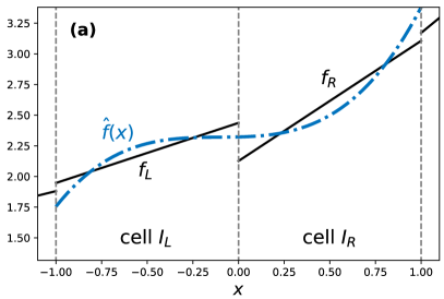
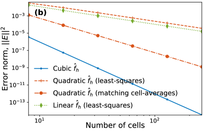
Figure 1: (a) A DG function (solid black) and its maximal order recovery polynomial (dash-dot blue). (b) Error norm in the $d^{2}(\sin x)/dx^{2}$ with cubic, quadratic and linear recovery.

The maximal-order recovery polynomial in (43) has fourth-order convergence (see figure (1b)), but it does not guarantee positivity. For systems in which $f$ must remain positive, using the highest order polynomial possible may lead to incursions below zero when $f$ is small. An example of this, due to both diffusion and advection, is illustrated in section 5. We explored computing second derivatives with lower order polynomials in order to see if positivity problems are minimized. The test function $f{=}\sin x$ in $x\in[-1,1]$ was discretized with piecewise polynomial bases ($p=1,~{}N_{p}=2$) which allows for a cubic maximal-order polynomial. We could also, instead of using (43), request a quadratic or a linear $\hat{f}$. In these two cases (3.1) leads to an over determined system that we solved by least squares. The error norms in the computation of $d^{2}(\sin x)/dx^{2}$ for all three recoveries are given in figure (1b) as a function of resolution. Unfortunately the convergence of these lower-order, least squares methods is inferior (closer to second order) and, in advection-diffusion problems, they were less stable. Also note that the quadratic least-squares $\hat{f}$ (dashed orange in figure (1b)) did not do any better than the linear $\hat{f}$ (dotted green in figure (1b)); a better procedure is to construct $\hat{f}$ by matching the cell-averages in each cell, and seeking the least-squares solution that tries to match the slopes in both cells (orange dash-dot in figure (1b)). In what follows, we use the maximal-order recovery polynomial and take other measures to decrease the likelihood of $f<0$.

3.2 Discrete GkLBO scheme

In order to discretize the GkLBO we project (7) onto the phase-space basis by multiplying by a test function $w\in\mathcal{V}_{3}^{p}$ and integrating over all phase-space:

$$\int_{\Omega_{i,j,k}}w\frac{\partial\mathcal{J}f}{\partial t}\thinspace\mathrm{d}x\thinspace\mathrm{d}v_{\parallel}\thinspace\mathrm{d}\mu=\nu\int_{\Omega_{i,j,k}}w\left\{\frac{\partial}{\partial v_{\parallel}}\left[(v_{\parallel}-u_{\parallel})\mathcal{J}f+v_{t}^{2}\frac{\partial\mathcal{J}f}{\partial v_{\parallel}}\right]+\frac{\partial}{\partial\mu}\left[2\mu\mathcal{J}f+2\frac{mv_{t}^{2}}{B}\mu\frac{\partial\mathcal{J}f}{\partial\mu}\right]\right\}\thinspace\mathrm{d}x\thinspace\mathrm{d}v_{\parallel}\thinspace\mathrm{d}\mu,$$ (45)

where we neglect the $2\pi/m$ integration factor to simplify notation. Integrate by parts once to give

$$\int_{\Omega_{i,j,k}}w\frac{\partial\mathcal{J}f}{\partial t}\thinspace\mathrm{d}x\thinspace\mathrm{d}v_{\parallel}\thinspace\mathrm{d}\mu =\nu\int_{x_{i-1/2}}^{x_{i+1/2}}\int_{\mu_{k-1/2}}^{\mu_{k+1/2}}w\,G_{v_{\parallel}}(f_{L},f_{R})\Bigg{|}_{v_{\parallel,j-1/2}}^{v_{\parallel,j+1/2}}\thinspace\thinspace\mathrm{d}x\thinspace\mathrm{d}\mu+\nu\int_{x_{i-1/2}}^{x_{i+1/2}}\int_{v_{\parallel,j-1/2}}^{v_{\parallel,j+1/2}}w\,G_{\mu}(f_{L},f_{R})\Bigg{|}_{\mu_{k-1/2}}^{\mu_{k+1/2}}\thinspace\thinspace\mathrm{d}x\thinspace\mathrm{d}v_{\parallel}$$ (46)

$$\quad-\nu\int_{\Omega_{i,j,k}}\left\{\frac{\partial w}{\partial v_{\parallel}}\left[(v_{\parallel}-u_{\parallel})\mathcal{J}f+v_{t}^{2}\frac{\partial\mathcal{J}f}{\partial v_{\parallel}}\right]+\frac{\partial w}{\partial\mu}\left[2\mu\mathcal{J}f+\frac{2mv_{t}^{2}}{B}\mu\frac{\partial\mathcal{J}f}{\partial\mu}\right]\right\}\thinspace\mathrm{d}x\thinspace\mathrm{d}v_{\parallel}\thinspace\mathrm{d}\mu.$$

The quantities $G_{v_{\parallel}}(f_{L},f_{R})$ and $G_{\mu}(f_{L},f_{R})$ are numerical fluxes chosen to preserve, in addition to conservation, other properties like stability and positivity. For example, the Lax-Friedrichs (LF) penalty fluxes are

$$G_{v_{\parallel}}(f_{L},f_{R}) =\frac{1}{2}(v_{\parallel}-u_{\parallel})(\mathcal{J}f_{R}+\mathcal{J}f_{L})-\frac{\tau_{v_{\parallel}}}{2}(\mathcal{J}f_{L}-\mathcal{J}f_{R})+v_{t}^{2}\frac{\partial\mathcal{J}\hat{f}}{\partial v_{\parallel}}$$ (47)

$$G_{\mu}(f_{L},f_{R}) =\mu(\mathcal{J}f_{R}+\mathcal{J}f_{L})-\frac{\tau_{\mu}}{2}(\mathcal{J}f_{L}-\mathcal{J}f_{R})+\frac{2mv_{t}^{2}}{B}\mu\frac{\partial\mathcal{J}\hat{f}}{\partial\mu},$$

where $\tau_{v_{\parallel}}=\max(|v_{\parallel}-u_{\parallel}|)$ and $\tau_{\mu}=\max(2\mu)$. The notation $f_{L}$ and $f_{R}$ refer to the distribution function in the left and right cells of a boundary, respectively. In section 4 we also discuss pure upwind fluxes which are more beneficial for positivity. Notice that the contribution to the numerical flux arising from the diffusion term is computed using the recovery polynomial described in section 3.1.

Additionally we impose the following boundary conditions on the numerical fluxes:

$$G_{v_{\parallel}}\left(f_{L}(v_{\parallel,\min}),f_{R}(v_{\parallel,\min})\right) =G_{v_{\parallel}}\left(f_{L}(v_{\parallel,\max}),f_{R}(v_{\parallel,\max})\right)=0,$$ (48)

$$G_{\mu}\left(f_{L}(0),f_{R}(0)\right) =G_{\mu}\left(f_{L}(\mu_{\max}),f_{R}(\mu_{\max})\right)=0.$$

The discrete form in (46)-(48) does not conserve momentum, shown by substituting $w=v_{\parallel}$ into (46) and summing over $v_{\parallel}$ space ($j$ index). The diffusion term in the volume integral can be integrated by parts again, yielding a surface term with non-vanishing jumps that breaks momentum conservation. A similar issue arises with energy conservation.

The conservation of $M_{0}$, $M_{1}$ and $M_{2}$ can be guaranteed if one integrates by parts twice and evaluates the additional surface terms using the recovered distribution function $\hat{f}$. Therefore the conservative GkLBO DG scheme follows

$$\int_{\Omega_{i,j,k}}w\frac{\partial\mathcal{J}f}{\partial t}\thinspace\mathrm{d}x\thinspace\mathrm{d}v_{\parallel}\thinspace\mathrm{d}\mu =\nu\int_{x_{i-1/2}}^{x_{i+1/2}}\int_{\mu_{k-1/2}}^{\mu_{k+1/2}}\left(w\,G_{v_{\parallel}}(f_{L},f_{R})-\frac{\partial w}{\partial v_{\parallel}}v_{t}^{2}\mathcal{J}\hat{f}\right)_{v_{\parallel,j-1/2}}^{v_{\parallel,j+1/2}}\thinspace\thinspace\mathrm{d}x\thinspace\mathrm{d}\mu$$ (49)

$$\quad+\nu\int_{x_{i-1/2}}^{x_{i+1/2}}\int_{v_{\parallel,j-1/2}}^{v_{\parallel,j+1/2}}\left(w\,G_{\mu}(f_{L},f_{R})-\frac{\partial w}{\partial\mu}2\frac{mv_{t}^{2}}{B}\mu\mathcal{J}\hat{f}\right)_{\mu_{k-1/2}}^{\mu_{k+1/2}}\thinspace\thinspace\mathrm{d}x\thinspace\mathrm{d}v_{\parallel}$$

$$\quad-\nu\int_{\Omega_{i,j,k}}\left\{\frac{\partial w}{\partial v_{\parallel}}(v_{\parallel}-u_{\parallel})-\frac{\partial^{2}w}{\partial v_{\parallel}^{2}}v_{t}^{2}+\frac{\partial w}{\partial\mu}2\mu-2\frac{mv_{t}^{2}}{B}\left(\mu\frac{\partial^{2}w}{\partial\mu^{2}}+\frac{\partial w}{\partial\mu}\right)\right\}\mathcal{J}f\,\thinspace\mathrm{d}x\thinspace\mathrm{d}v_{\parallel}\thinspace\mathrm{d}\mu.$$

We continue to assume a $2\pi/m$ factor in front of the $\mu$ integral. The conservative properties of the discrete operator are proven below.

3.2.1 Number Density Conservation:

Scheme 49 conserves number density:

$$\frac{d}{dt}\sum_{j,k}\int_{\Omega_{i,j,k}}\mathcal{J}f\thinspace\mathrm{d}x\thinspace\mathrm{d}v_{\parallel}\thinspace\mathrm{d}\mu=0.$$ (50)

In order to show this use $w=1$ in (49) and sum over all velocity space cells. The sum need not be over configuration space as the configuration space gradients only occur in the collisionless terms of the gyrokinetic equation. The numerical flux is continuous across interior cell surfaces, so those contributions cancel. Only global the fluxes at the boundaries of velocity space remain, but those are zero given the boundary conditions in (48).

3.2.2 Discrete Momentum Conservation:

Scheme 49 conserves momentum:

$$\frac{d}{dt}\sum_{j,k}\int_{\Omega_{i,j,k}}v_{\parallel}\mathcal{J}f\thinspace\mathrm{d}x\thinspace\mathrm{d}v_{\parallel}\thinspace\mathrm{d}\mu=0,$$ (51)

if the following weak-equality relation is satisfied:

$$u_{\parallel}M_{0}-v_{t}^{2}\sum_{k}\int_{\mu_{k-1/2}}^{\mu_{k+1/2}}\left(\mathcal{J}f(v_{\parallel,\max})-\mathcal{J}f(v_{\parallel,\min})\right)\thinspace\mathrm{d}\mu\doteq M_{1}.$$ (52)

One can show momentum conservation and arrive at this constraint using $w=v_{\parallel}$ in (49) and summing over all velocity space cells to get

$$\frac{d}{dt}\sum_{j,k}\int_{\Omega_{i,j,k}}v_{\parallel}\mathcal{J}f\thinspace\mathrm{d}x\thinspace\mathrm{d}v_{\parallel}\thinspace\mathrm{d}\mu=-\nu\sum_{j,k}\int_{x_{i-1/2}}^{x_{i+1/2}}\int_{\mu_{k-1/2}}^{\mu_{k+1/2}}v_{t}^{2}\mathcal{J}\hat{f}\thinspace\mathrm{d}x\thinspace\mathrm{d}\mu\Bigg{|}_{v_{\parallel,j-1/2}}^{v_{\parallel,j+1/2}}-\nu\sum_{j,k}\int_{\Omega_{i,j,k}}(v_{\parallel}-u_{\parallel})\mathcal{J}f\,\thinspace\mathrm{d}x\thinspace\mathrm{d}v_{\parallel}\thinspace\mathrm{d}\mu$$ (53)

The contributions from the numerical fluxes $G_{v_{\parallel}}$ and $G_{\mu}$ drop out due to continuity and boundary conditions. In the first term all interface contributions from $v_{\parallel}$ will cancel except the first and last. Combined with the definition of the discrete moments in the second term leads to the constraint

$$\int_{x_{i-1/2}}^{x_{i+1/2}}\left[\sum_{k}\int_{\mu_{k-1/2}}^{\mu_{k+1/2}}v_{t}^{2}\left(\mathcal{J}\hat{f}(v_{\parallel,\max})-\mathcal{J}\hat{f}(v_{\parallel,\min})\right)\thinspace\mathrm{d}\mu+M_{1}-u_{\parallel}M_{0}\right]\thinspace\mathrm{d}x=0.$$ (54)

Using the definition of weak equality, this implies that the momentum will be conserved if (52) is satisfied. Notice that $\hat{f}$ was replaced by $f$ because at the outer velocity boundaries there is no “outside” cell to allow for recovery of a continuous distribution function.

The weak-equality constraint (52) is stronger than what is required by (54). However, ensuring that the weak-equality constraint is satisfied automatically ensures that momentum conservation is preserved. For simplicity we assume a unit mass $m=1$ in what follows, with no loss of generality.

3.2.3 Discrete Energy Conservation:

Scheme 49 conserves energy

$$\frac{d}{dt}\sum_{j,k}\int_{\Omega_{i,j,k}}\left(\frac{1}{2}v_{\parallel}^{2}+\mu B\right)\mathcal{J}f\thinspace\mathrm{d}x\thinspace\mathrm{d}v_{\parallel}\thinspace\mathrm{d}\mu=0,$$ (55)

if the following weak-equality relation is satisfied:

$$u_{\parallel}M_{1}+v_{t}^{2} \left[3M_{0}-\sum_{k}\int_{\mu_{k-1/2}}^{\mu_{k+1/2}}\left(v_{\parallel,\max}\mathcal{J}f(v_{\parallel,\max})-v_{\parallel,\min}\mathcal{J}f(v_{\parallel,\min})\right)\thinspace\mathrm{d}\mu\right.$$ (56)

$$\left.\quad\quad\hskip 3.0pt-\sum_{j}\int_{v_{\parallel,j-1/2}}^{v_{\parallel,j+1/2}}2\left(\mu_{\max}\mathcal{J}f(\mu_{\max})-\mu_{\min}\mathcal{J}f(\mu_{\min})\right)\thinspace\mathrm{d}v_{\parallel}\right]\doteq M_{2}.$$

Assuming that $p\geq 2$ such that $v^{2}\in\mathcal{V}_{2}^{p}$, the above two equations follow from replacing $w=v_{\parallel}^{2}/2+\mu B$ in (49) and summing over all velocity space cells, which yields

$$\frac{d}{dt}\sum_{j,k}\int_{\Omega_{i,j,k}}\frac{1}{2}v^{2}\mathcal{J}f\thinspace\mathrm{d}x\thinspace\mathrm{d}v_{\parallel}\thinspace\mathrm{d}\mu =-\nu\sum_{j,k}\int_{x_{i-1/2}}^{x_{i+1/2}}\left(\int_{\mu_{k-1/2}}^{\mu_{k+1/2}}v_{t}^{2}v_{\parallel}\mathcal{J}\hat{f}\thinspace\Bigg{|}_{v_{\parallel,j-1/2}}^{v_{\parallel,j+1/2}}\thinspace\mathrm{d}\mu+\int_{v_{\parallel,j-1/2}}^{v_{\parallel,j+1/2}}2v_{t}^{2}\,\mu\mathcal{J}\hat{f}\thinspace\Bigg{|}_{\mu_{k-1/2}}^{\mu_{k+1/2}}\thinspace\mathrm{d}v_{\parallel}\right)\thinspace\mathrm{d}x$$

$$\quad-\nu\sum_{j,k}\int_{\Omega_{i,j,k}}\left[v_{\parallel}(v_{\parallel}-u_{\parallel})+2\mu B-3v_{t}^{2}\right]\mathcal{J}f\thinspace\mathrm{d}x\thinspace\mathrm{d}v_{\parallel}\thinspace\mathrm{d}\mu.$$

All contributions from interior cell interfaces cancel in the first term. Velocity-space integrals in the second term can be written in terms of discrete moments, leading to the following constraint in order to have energy conservation:

$$\int_{x_{i-1/2}}^{x_{i+1/2}}\left[\sum_{k}\int_{\mu_{k-1/2}}^{\mu_{k+1/2}}v_{t}^{2}\left(v_{\parallel,\max}\mathcal{J}\hat{f}(v_{\parallel,\max})-v_{\parallel,\min}\mathcal{J}\hat{f}(v_{\parallel,\min})\right)\thinspace\mathrm{d}\mu\right.$$ (57)

$$\left.\quad\qquad+\sum_{j}\int_{v_{\parallel,j-1/2}}^{v_{\parallel,j+1/2}}2v_{t}^{2}\left(\mu_{\max}\mathcal{J}\hat{f}(\mu_{\max})-\mu_{\min}\mathcal{J}\hat{f}(\mu_{\min})\right)\thinspace\mathrm{d}v_{\parallel}+M_{2}-u_{\parallel}M_{1}-3v_{t}^{2}M_{0}\right]\thinspace\mathrm{d}x=0.$$

Using the definition of weak equality this implies that the energy will be conserved if (56) is satisfied.

Thus, exact $p\geq 2$ conservation of momentum and energy leads to the following set of weak-equality relations:

$$u_{\parallel}M_{0}-v_{t}^{2}\frac{2\pi}{m}\sum_{k}\int_{\mu_{k-1/2}}^{\mu_{k+1/2}}\mathcal{J}f\thinspace\Big{|}^{v_{\parallel,\max}}_{v_{\parallel,\min}}\thinspace\mathrm{d}\mu\doteq M_{1},$$ (58)

$$u_{\parallel}M_{1}+v_{t}^{2}\left[3M_{0}-\frac{2\pi}{m}\sum_{k}\int_{\mu_{k-1/2}}^{\mu_{k+1/2}}v_{\parallel}\mathcal{J}f\thinspace\Big{|}^{v_{\parallel,\max}}_{v_{\parallel,\min}}\thinspace\mathrm{d}\mu-\frac{2\pi}{m}\sum_{j}\int_{v_{\parallel,j-1/2}}^{v_{\parallel,j+1/2}}2\mu\mathcal{J}f\thinspace\Big{|}^{\mu_{\max}}_{\mu_{\min}}\thinspace\mathrm{d}v_{\parallel}\right]\doteq M_{2},$$

where we restored the $2\pi/m$ factors for clarity. This is a weak linear system of equations that needs to be inverted in every cell of the configuration-space grid to compute the parallel drift velocity $u_{\parallel}$ and the thermal speed $v_{t}$. Without the boundary corrections presented above, the errors in the conserved quantities are several orders of magnitude higher. Also, instabilities can be observed when velocity-grid extents are too low and $f$ is appreciable at the boundary.

3.2.4 Discrete p=1 Energy Conservation:

The above energy conservation theorem applied to $p\geq 2$ basis functions which span the quadratic term in the test function $v_{\parallel}^{2}/2+\mu B$. For a piecewise linear basis ($p=1$), conservation can be maintained in the sense that we can conserve the projection of the second moment $M_{2}$ onto the piecewise linear basis. This property can be ensured if the quadratic term in the test function is replaced by its projection onto the basis functions, $\overline{v_{\parallel}^{2}}\in\mathcal{V}_{3}^{1}$, which is weakly equivalent to $v_{\parallel}^{2}$ in this basis:

$$\overline{v_{\parallel}^{2}}\doteq v_{\parallel}^{2}\quad\mathrm{on}\;\mathcal{V}_{3}^{1}.$$ (59)

It is straightforward to show that $\overline{v_{\parallel}^{2}}$ is continuous. Also, in a weak-equality sense, the definition of particle energy is the same, whether we use the original quadratic expression or its projection. Therefore we can show that scheme 49 satisfies

$$\frac{d}{dt}\sum_{j,k}\int_{\Omega_{i,j,}}(v_{\parallel}^{2}/2+\mu B)\thinspace\mathcal{J}f\thinspace\mathrm{d}x\thinspace\mathrm{d}v_{\parallel}\thinspace\mathrm{d}\mu=0,$$ (60)

with a piecewise linear basis as long as the following weak equality is satisfied:

$$u_{\parallel}M^{*}_{1}+v_{t}^{2} \left[M^{*}_{0}+2M_{0}-\sum_{k}\int_{\mu_{k-1/2}}^{\mu_{k+1/2}}\left(\check{v}_{\parallel,\max}\mathcal{J}f(v_{\parallel,\max})-\check{v}_{\parallel,\min}\mathcal{J}f(v_{\parallel,\min})\right)\mathrm{d}\mu\right.$$ (61)

$$\left.\qquad\qquad-\sum_{j}\int_{v_{\parallel,j-1/2}}^{v_{\parallel,j+1/2}}2\left(\mu_{\max}\mathcal{J}f(\mu_{\max})-\mu_{\min}\mathcal{J}f(\mu_{\min})\right)\mathrm{d}v_{\parallel}\right]\doteq M^{*}_{2}.$$

where $\check{v}_{\parallel,j}=(v_{\parallel,j+1/2}+v_{\parallel,j-1/2})/2$, $\Delta v_{\parallel,j}=\check{v}_{\parallel,j+1}-\check{v}_{\parallel,j}$ and the “star moments” are defined as

$$M^{*}_{0} \doteq\sum_{j\neq j_{\max}}\sum_{k}\int_{\mu_{k-1/2}}^{\mu_{k+1/2}}\Delta v_{\parallel,j}\thinspace\mathcal{J}\hat{f}_{j+1/2}\,\mathrm{d}\mu$$ (62)

$$M^{*}_{1} \doteq\sum_{j,k}\int_{v_{\parallel,j-1/2}}^{v_{\parallel,j+1/2}}\int_{\mu_{k-1/2}}^{\mu_{k+1/2}}\check{v}_{\parallel,j}\thinspace\mathcal{J}f\,\thinspace\mathrm{d}v_{\parallel}\thinspace\mathrm{d}\mu$$

$$M^{*}_{2} \doteq\sum_{j,k}\int_{v_{\parallel,j-1/2}}^{v_{\parallel,j+1/2}}\int_{\mu_{k-1/2}}^{\mu_{k+1/2}}(\check{v}_{\parallel,j}v_{\parallel}+2\mu B)\thinspace\mathcal{J}f\thinspace\thinspace\mathrm{d}v_{\parallel}\thinspace\mathrm{d}\mu.$$

The argument leading to 60-62 begins with using the projection $\overline{v_{\parallel}^{2}}/2$ (59) in showing conservation of the energy, since $v_{\parallel}^{2}/2\notin\mathcal{V}_{3}^{1}$. This means setting $w=\overline{v_{\parallel}^{2}}/2+\mu B$ in (49) and summing over all velocity space cells. Aided by the fact that

$$\frac{\partial}{\partial v_{\parallel}}\left(\frac{1}{2}{\overline{v_{\parallel}^{2}}}\right)=\frac{1}{2}(v_{\parallel,j+1/2}+v_{\parallel,j-1/2})\equiv\check{v}_{\parallel,j}.$$ (63)

one then arrives at

$$\frac{d}{dt}\sum_{j,k}\int_{\Omega_{i,j,k}}(v_{\parallel}^{2}/2+\mu B)\thinspace\mathcal{J}f\thinspace\mathrm{d}x\thinspace\mathrm{d}v_{\parallel}\thinspace\mathrm{d}\mu =-\nu\sum_{j,k}\int_{x_{i-1/2}}^{x_{i+1/2}}\left(\int_{\mu_{k-1/2}}^{\mu_{k+1/2}}\check{v}_{\parallel,j}v_{t}^{2}\mathcal{J}\hat{f}\thinspace\Bigg{|}_{v_{\parallel,j-1/2}}^{v_{\parallel,j+1/2}}\mathrm{d}\mu+\int_{v_{\parallel,j-1/2}}^{v_{\parallel,j+1/2}}2v_{t}^{2}\,\mu\mathcal{J}\hat{f}\,\Bigg{|}_{\mu_{k-1/2}}^{\mu_{k+1/2}}\mathrm{d}v_{\parallel}\right)\mathrm{d}x$$ (64)

$$\quad-\nu\sum_{i,j}\int_{\Omega_{i,j,k}}\left[\check{v}_{\parallel,j}(v_{\parallel}-u_{\parallel})+2\mu B-2v_{t}^{2}\right]\mathcal{J}f\thinspace\mathrm{d}x\thinspace\mathrm{d}v_{\parallel}\thinspace\mathrm{d}\mu.$$

The terms containing the numerical flux $G_{v_{\parallel}}$ drop out since $\overline{v_{\parallel}^{2}}/2$ is continuous and we are enforcing zero-flux boundary conditions in velocity-space (and so does the $G_{\mu}$ term). However, as $\check{v}_{\parallel,j}$ is not continuous the contribution from the first term in (64) does not drop out. This term can be written as

$$\int_{x_{i-1/2}}^{x_{i+1/2}}v_{t}^{2}\sum_{j,k}\int_{\mu_{k-1/2}}^{\mu_{k+1/2}}\check{v}_{\parallel,j}\mathcal{J}\hat{f}\Bigg{|}_{v_{\parallel,j-1/2}}^{v_{\parallel,j+1/2}}\thinspace\thinspace\mathrm{d}x\thinspace\mathrm{d}\mu=\int_{x_{i-1/2}}^{x_{i+1/2}}\sum_{k}\int_{\mu_{k-1/2}}^{\mu_{k+1/2}} \left[v_{t}^{2}\left(\check{v}_{\parallel,\max}\mathcal{J}f(v_{\parallel,\max})-\check{v}_{\parallel,\min}\mathcal{J}f(v_{\parallel,\min})\right)\right.$$ (65)

$$\left.\quad-v_{t}^{2}\sum_{j\neq j_{\max}}\Delta v_{\parallel,j}\mathcal{J}\hat{f}_{j+1/2}\right]\thinspace\thinspace\mathrm{d}x\thinspace\mathrm{d}\mu.$$

Utilizing the star moments in (62) and the definition of weak equality, this last relation implies that the energy will be conserved in the $p=1$ case if (61) is satisfied.

In summary, for piecewise linear bases the drift velocity and thermal speed must be determined using the following set of linear weak-equality relations

$$u_{\parallel}M_{0} -v_{t}^{2}\frac{2\pi}{m}\sum_{k}\int_{\mu_{k-1/2}}^{\mu_{k+1/2}}\mathcal{J}f\thinspace\Big{|}^{v_{\parallel,\max}}_{v_{\parallel,\min}}\thinspace\mathrm{d}\mu\doteq M_{1},$$ (66)

$$u_{\parallel}M^{*}_{1} +v_{t}^{2}\left\{M^{*}_{0}+2M_{0}-\frac{2\pi}{m}\left[\sum_{k}\int_{\mu_{k-1/2}}^{\mu_{k+1/2}}\left(\check{v}_{\parallel,\max}\mathcal{J}f(v_{\parallel,\max})-\check{v}_{\parallel,\min}\mathcal{J}f(v_{\parallel,\min})\right)\mathrm{d}\mu\right.\right.$$

$$\left.\left.\qquad\qquad\qquad\qquad\quad+2\sum_{j}\int_{v_{\parallel,j-1/2}}^{v_{\parallel,j+1/2}}\mu\mathcal{J}f\thinspace\Big{|}^{\mu_{\max}}_{\mu_{\min}}\mathrm{d}v_{\parallel}\right]\right\}\doteq M^{*}_{2}.$$

We have again reinstated the $2\pi/m$ factors for completeness. Notice that this weak system requires computing the first two regular moments ($M_{0}$ and $M_{1}$) and the three star moments.

4 Time-stepping and stability

A high-order, conservative DG scheme for the GkLBO must be accompanied by a suitable time-stepping scheme. In this section we complement the spatial discretization of the gyrokinetic-GkLBO equation presented in sections 2-3, and that of the Vlasov-Maxwell-Dougherty system presented in [22], with a description of the time-stepping algorithm and its stability. As a preliminary, recall that one can determine the appropriate time-step (${\Delta}t$) for a linear problem $df/dt=\mathrm{L}[f]$ by estimating the eigenvalues $\lambda$ of the operator $\mathrm{L}$. Then the time-step is chosen such that $\lambda{\Delta}t$ is within the region of numerical stability for a particular time-stepping algorithm for all eigenvalues of the operator [31].

Purely damped modes, those for which $df/dt=\lambda f$ and $\lambda<0$, will be stable when using an individual Euler step if $\left|\lambda\right|{\Delta}t<2$ because $f^{n+1}=(1+\lambda{\Delta}t)f^{n}$ (where the $n$ exponent labels the $n$-th time step). In Gkeyll we instead use an explicit third-order Strong Stability Preserving (SSP) Runge-Kutta (SSP-RK3) with convex combinations of individual Euler steps that has a combined stability limit of $\left|\lambda_{\mathrm{max}}\right|{\Delta}t\lesssim 2.512$ for purely damped modes, as can also be seen in figure 2.4 in [31]. One may instead wish to ensure the stability of each Euler stage and avoid “overdamped” solutions that oscillate around zero (instead of just damping with the same sign) by using the more conservative limit $\left|\lambda\right|{\Delta}t<1$.

Although the GkLBO is nonlinear we can use these ideas to estimate stability limits of the drag and diffusion terms separately. We will then combine these into a single rule for choosing the time step for the whole GkLBO, and discuss the additional considerations brought about by the collisionless terms. We add that for collision-dominated regimes explicit time-stepping will not be sufficiently efficient, and one may need to use an implicit scheme instead. One option we intend to explore in the future is to use super-time-steppers [32] to overcome this obstacle.

4.1 Stability of a DG Advection Operator

The stability limits of the GkLBO drag term can be probed by examining the advection equation $\partial f/\partial t=-v\partial f/\partial x$. The lowest order ($p=0$) DG is equivalent to a first-order upwind finite volume algorithm, which for $v>0$ gives the solution in the $j$-th cell as

$$\frac{\partial f_{j}}{\partial t}=-v\frac{f_{j}-f_{j-1}}{\Delta x}.$$ (67)

One can substitute the eigenfunction $f_{j}(t)=A(t){\rm e}^{ikx_{j}}$ and find that the maximum eigenvalue occurs for $k=\pi/\Delta x$, the Nyquist mode. This simplifies the above equation to $\partial A/\partial t=-2vA/\Delta x$ and hence the largest absolute magnitude of the eigenvalue is

$$\lambda_{\mathrm{max}}=\frac{2v}{\Delta x}\quad\mathrm{for}~{}p=0.$$ (68)

As mentioned earlier the stability limit of a first-order Euler step is $|\lambda|{\Delta}t<2$ (see figure 2.4 in [31]). Using (68), this condition can be expressed in terms of a Courant-Lewy-Friedrichs ($\mathrm{CFL}$) number as $v{\Delta}t/\Delta x=\mathrm{CFL}<1$. Requiring every Euler stage of a SSP-RK3 method to satisfy this constraint can be overly conservative, and one could, in principle, use a slightly larger time-step, as described above, $\lambda_{\mathrm{max}}\Delta t<2.512$, which corresponds to $\mathrm{CFL}<1.256$.

For piecewise linear DG ($p=1$), the maximum eigenvalue is somewhat larger. In general one can do a von Neuman-type analysis assuming the solutions between cells varies like $e^{ikx}$, and calculate the spectrum of eigenvalues of the DG discretization of the $d/dx$ operator as a function of wavenumber $k$, from $k=0$ up to $k=k_{\rm max}=(p+1)\pi/(\Delta x)_{\rm cell}$, where the extended $k$ domain accounts for the $(p+1)$ degrees of freedom within each DG cell that effectively provide a finer mesh than the cell width. We will assume, as is true for $p=2$, that the stability limit is set by the Nyquist mode, $k=k_{\rm max}$. In the $j$-th cell the Nyquist mode for $p=1$ has a mean value of 0 (so $f_{j0}=0$) and a linear slope $f_{j}(x,t)=f_{j1}(t)\psi_{1}(x-x_{j})$, where $\psi_{1}(x)=\sqrt{3}x/(\Delta x/2)$ is an orthonormal basis function. Then the evolution of the DG representation of this mode is

$$\frac{\partial f_{1}}{\partial t} =-v\,{\left\langle\psi_{1},\frac{\partial f}{\partial x}\right\rangle}=-\frac{v\sqrt{3}}{\Delta x}\big{(}\hat{F}(\Delta x/2)+\hat{F}(-\Delta x/2)\big{)}$$ (69)

$$=-6\frac{v}{\Delta x}f_{1},$$

where $v\hat{F}$ is the upwind numerical flux at the cell boundaries. In this case, the eigenvalue is

$$\lambda_{\rm max}=6\frac{v}{\Delta x}_{\rm cell}.$$ (70)

Equations 68 and 70 are fit perfectly by the formula $\lambda_{\mathrm{max}}=2(2p+1)v/\Delta x_{\mathrm{cell}}$. However, for piecewise quadratic basis functions ($p=2$), one finds that $\lambda_{\mathrm{max}}\approx 11.9\,v/\Delta x_{\mathrm{cell}}$. (This is done by solving for the $\lambda$ spectrum of the DG discretization of $\partial/\partial x$ which, for $p=2$, requires solving a $3\times 3$ linear system.) The resulting general formula for the maximum eigenvalue for advection is

$$\lambda_{\mathrm{adv}}=2\,C_{\mathrm{adv},p}\,(2p+1)\max(v/\Delta x_{\mathrm{cell}}),$$ (71)

where the advection coefficient is $C_{\mathrm{adv},p}=\{1,1,1.2\}$ for $p=\{0,1,2\}$, respectively. For RK3 $\lambda_{\rm max}\Delta t<2.512$ gives a time step limit of $v\Delta t/\Delta x_{\rm cell}<\{1.256,\,0.418,\,0.209\}$ for $p=\{0,1,2\}$, which is within 3% of the empirically determined numbers in Table 2.2 of [33]. Note that an equivalent finite-difference/finite-volume mesh with the same number of degrees of freedom would have an effective grid spacing $\Delta x_{\rm eff}=\Delta x_{\rm cell}/(p+1)$, so the stability limit on the time step in terms of an effective Courant number is $v\Delta t/\Delta x_{\rm eff}<1.256\,(p+1)/(C_{adv,p}(2p+1))=\{1.256,\,0.836,\,0.627\}$ for $p=\{0,1,2\}$, which does not drop as quickly at higher $p$ as a Courant number $v\Delta t/\Delta x_{\rm cell}$ expressed in terms of cell width.

4.2 Stability of a DG diffusion operator

Consider the diffusion equation $\partial f/\partial t=D\partial^{2}f/\partial x^{2}$. In second-order centered finite-difference (equivalent to finite-volume) discretizations of this operator the largest magnitude eigenvalue is $\lambda_{\mathrm{max}}=-4D/(\Delta x)^{2}$ when using a forward Euler step. This is the $p=0$ limit of DG, and one might attempt to employ the same formula but with the effective DG cell length $\Delta x=\Delta x_{\mathrm{cell}}/(2p+1)$ that was used for advective terms. For a parabolic term (diffusion) it turns out that $\Delta x=\Delta x_{\mathrm{cell}}/(p+1)$ is more accurate. van Leer and Nomura calculate the eigenmodes and eigenvalues of a diffusion operator using RDG with $p=1$ and $p=2$ [28]. Their equation 79 and figure 1 give $\lambda_{\mathrm{max}}=15/(\Delta x_{\mathrm{cell}})^{2}$ for $p=1$, while their figure 3 gives $\lambda_{\mathrm{max}}\approx 33/(\Delta x_{\mathrm{cell}})^{2}$ for $p=2$. These results can be fit with the expression

$$\lambda_{d}=-4C_{\mathrm{dif},p}D\left(\frac{p+1}{\Delta x_{\mathrm{cell}}}\right)^{2}.$$ (72)

where $C_{\mathrm{dif},p}=\{1,0.94,0.92\}$ for $p=\{0,1,2\}$, respectively.

4.3 Stability of the nonlinear model-Fokker-Planck operator

The spatial discretization of the Vlasov-Dougherty equation discussed in [22] can use the same estimates for the SSP-RK3 ${\Delta}t$ as those for the one-velocity-dimension GkLBO. Such limit of (7) is

$$\frac{\partial\mathcal{J}f}{\partial t}=\mathcal{J}\mathcal{C}[f]=\frac{\partial}{\partial v_{\parallel}}\left[\nu(v_{\parallel}-u_{\parallel})\mathcal{J}f+\nu v_{t}^{2}\frac{\partial\mathcal{J}f}{\partial v_{\parallel}}\right].$$ (73)

The first term looks like an advection term, so one might think that it gives an imaginary part to the eigenvalues. However, the eigenvalues of the full collision operator are not necessarily a simple sum of the separate eigenvalues of the diffusion and advection terms. We have already noted in section 2 that the combined drag and diffusion terms in the continuous GkLBO have a set of eigenmodes that are all purely damped (real $\lambda<0$).

For now we use a conservative estimate of the eigenvalues of the DG-discretized GkLBO based on a sum of contributions from the advection and diffusions terms. We use $\Delta v_{\parallel}=\Delta v_{\parallel,\mathrm{cell}}/(2p+1)$ for the advection term and $\Delta v_{\parallel}=\Delta v_{\parallel,\mathrm{cell}}/(p+1)$ for the diffusion term. Assuming a constant grid spacing, the estimated maximum eigenvalue of the GkLBO is

$$\left|\lambda_{\mathrm{max}}\right|=2\nu C_{\mathrm{adv},p}\max(|v_{\parallel}-u_{\parallel}|)\frac{(2p+1)}{\Delta v_{\parallel,\mathrm{cell}}}+4\nu C_{\mathrm{dif},p}v_{t}^{2}\left(\frac{p+1}{\Delta v_{\parallel,\mathrm{cell}}}\right)^{2}.$$ (74)

This can be generalized to higher dimensions without difficulty. For the 1X2V (one configuration-space dimension, and two velocity-space dimensions) GkLBO we use the following maximum eigenvalue estimate

$$\left|\lambda_{\mathrm{max}}\right|= 2\nu C_{\mathrm{adv},p}(2p+1)\left[\frac{\max(|v_{\parallel}-u_{\parallel}|)}{\Delta v_{\parallel,\mathrm{cell}}}+\frac{2\mu_{\max}}{\Delta\mu_{\mathrm{cell}}}\right]+4\nu C_{\mathrm{dif},p}v_{t}^{2}\left(p+1\right)^{2}\left[\frac{1}{\left(\Delta v_{\parallel,\mathrm{cell}}\right)^{2}}+\frac{m}{B}\frac{2\mu_{\max}}{\left(\Delta\mu_{\mathrm{cell}}\right)^{2}}\right].$$ (75)

This eigenvalue is computed every stage of the SSP-RK3 and used to calculate the time step according to ${\Delta}t|\lambda_{\mathrm{{GkLBO}}}|<\mathrm{CFL}$. The $\mathrm{CFL}$ number is close to unity, but in Gkeyll it can be modified as a user input.

In order to illustrate the impact of these choices consider the spatially homogeneous relaxation problem in 1X1V posed by (73) with a bump-on-tail distribution function for its initial condition:

$$f(t=0)=f_{M}(n,u_{\parallel},v_{t})+f_{M}(n,u_{\parallel,b},v_{t,b})\frac{a_{b}^{2}}{(v_{\parallel}-u_{\parallel,b})^{2}+s_{b}^{2}}.$$ (76)

Here $f_{M}(n,u_{\parallel},v_{t})$ is the one velocity-space dimension Maxwellian

$$f_{M}(n,u_{\parallel},v_{t})=\frac{n}{\sqrt{2\pi v_{t}^{2}}}\exp\left[-\frac{\left(v_{\parallel}-u_{\parallel}\right)^{2}}{2v_{t}^{2}}\right],$$ (77)

and we employed the parameters $n=1$, $u_{\parallel}=0$, $v_{t}=1/3$, $a_{b}=\sqrt{0.1}$, $u_{\parallel,b}=6v_{t}/\sqrt{3}$, $v_{t,b}=1.0$ and $s_{b}=0.12$. This distribution is discretized in a $[0,1]\times[-8v_{t},8v_{t}]$ domain using $2\times 32$ cells and a pieceswise linear basis ($p=1$), or $2\times 16$ and a piecewise quadratic basis ($p=2$). Using a collisionality of $\nu=0.01$ we show that by time $t=\nu^{-1}$ the GkLBO relaxes this initial condition to be close to a Maxwellian (figure (2)). By gradually increasing the CFL for each test, we discovered that for piecewise linear basis functions ($p=1$) the simulation begins to become unstable for $\mathrm{CFL}\gtrsim 1.431$, which gives ${\Delta}t\approx 0.075726$. Oscillations are observed close to or below zero in regions where $f$ is small (inset of figure (2a)), and the simulation diverges at later time. Piecewise quadratic basis functions ($p=2$) allowed $\mathrm{CFL}\lesssim 2.051$, corresponding to ${\Delta}t\approx 0.062479$ (figure (2)). The fact that these two cases ($p=1,2$) were not stable all the way up to ${\rm CFL}=\gamma_{\rm max}\Delta t<2.512$ (the stability limit for RK3 for damped modes) indicates that there are some inaccuracies in the approximations that led to Eq. 75, such as in treating advection and diffusion separately or in neglecting boundary conditions. Nevertheless, it captures the main scaling of the allowable time step with the parameters of the problem.

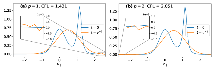
Figure 2: Relaxation of a 1X1V bump-on-tail distribution with (a) $p=1$ and (b) $p=2$ using the minimum $\mathrm{CFL}$ at which an instability is found. Unstable oscillations are seen at the edges of the domain, which grow quickly if the simulations are run for longer times.

Similar oscillations are observed in 1X2V simulations. We projected (76) onto the 1X2V DG basis, using the Maxwellian $f_{M}(n,u_{\parallel},v_{t})$ defined in (25), with parameters $v_{t}=1/\sqrt{12}$, $v_{t,b}=1/\sqrt{2}$, and $u_{b}=4v_{t}$. The bump-on-tail initial condition is relaxed to a Maxwellian within one collisional period (compare figures (3a) with figures(3b) and (3c)). The domain in these plots is $[0,1]\times[-v_{\parallel,\max},v_{\parallel,\max}]\times[0,mv_{\parallel,\max}^{2}/(2B)]$ with $v_{\parallel,\max}=6.93v_{t}$, $m=1$, $B=1$ and using $2\times 32\times 16$ cells for $p=1$, or $2\times 16\times 8$ cells for $p=2$. As $\mathrm{CFL}$ increases, an instability begins to develop at $\mathrm{CFL}=1.984$ for $p=1$ (${\Delta}t\approx 0.063075$), and $\mathrm{CFL}=2.298$ for $p=2$ (${\Delta}t\approx 0.075544$). It is difficult to discern in figures (3b-c), but figure (3d) shows a slice at $f(x=0.5,v_{\parallel},\mu=\mu_{\max})$ exhibiting oscillations near the boundary with regions of $f<0$.

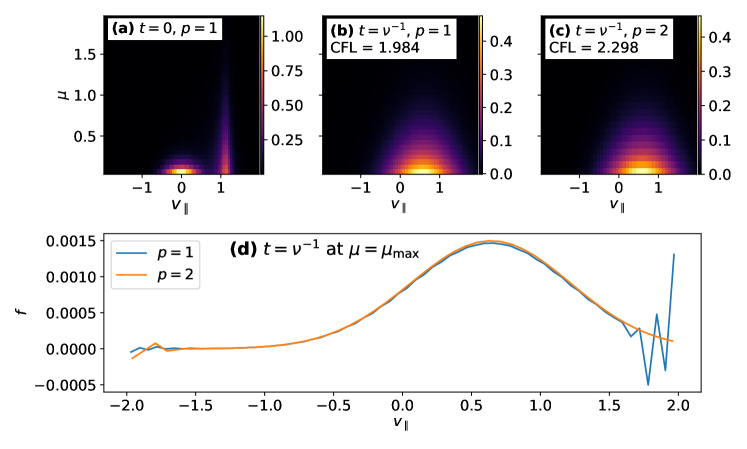
Figure 3: (a) Initial 1X2V bump-on-tail distribution. GkLBO relaxation of such initial condition with (b) $p=1$ and (c) $p=2$, using the minimum unstable $\mathrm{CFL}$. (d) Demonstration of the instability beginning to form near the right (left) boundary for $p=1$ ($p=2$) at a slice through $\mu=\mu_{\max}$ and $t=\nu^{-1}$ when the minimum unstable CFL is used.

The errors illustrated above are eliminated by more conservative $\mathrm{CFL}$ choices, yet another area of concern is positivity of the distribution function. Note that negative $f$ values do not always immediately give way to numerical instabilities. An example of this resilience is illustrated by relaxing the rectangular distribution

$$f(t{=}0,x,v_{\parallel},\mu)=\begin{cases}1/(2\pi v_{0}^{3})\qquad|v_{\parallel}|\leq v_{0}~{}\mathrm{and}~{}\mu\leq mv_{0}^{2}/(2B)\\ 0\qquad|v_{\parallel}|>v_{0}~{}\mathrm{or}~{}\mu>mv_{0}^{2}/(2B),\end{cases}$$ (78)

where $v_{0}=1/\sqrt{6}$, $m=1$ and $B=1$, on a coarse mesh of $4\times 32^{2}$ cells in the domain $[0,1]\times[-v_{\parallel,\max},v_{\parallel,\max}]\times[0,mv_{\parallel,\max}^{2}/(2B)]$, using $v_{\parallel,\max}=16v_{0}^{2}$. With these parameters the $\mu$ direction is under-resolved, such that after a collisional period the rapid drop in $f$ at small $\mu$ is hard to capture with a piecewise linear basis. The result, as shown by the dotted orange line in figure (4), is that the solution overshoots near zero and causes regions of $f<0$. This can be problematic as it can lead to unphysical, local negative densities and temperatures. However, on this occasion the code remains stable and the relaxation proceeds without a problem; this is the maximum entropy solution. In section 3.1 we commented on how RDG for the diffusion operator can lead to regions of $f<0$, and unfortunately lower order recovery polynomials did not provide a satisfactory solution (figure (1b)). Positivity is better respected by using local Lax-Friedrichs (LF) fluxes: instead of the fluxes in (47) with the maximum evaluated over the global domain (global LF fluxes), we can use

$$G_{v_{\parallel}}(f_{L},f_{R}) =(v_{\parallel}-u_{\parallel})\left\{\frac{1}{2}(\mathcal{J}f_{R}+\mathcal{J}f_{L})-\frac{\mathrm{sgn}\left[(v_{\parallel}-u_{\parallel})\hat{v_{\parallel}}\cdot\hat{n}\right]}{2}(\mathcal{J}f_{L}-\mathcal{J}f_{R})\right\}+v_{t}^{2}\frac{\partial\mathcal{J}\hat{f}}{\partial v_{\parallel}},$$ (79)

$$G_{\mu}(f_{L},f_{R}) =2\mu\left[\frac{1}{2}(\mathcal{J}f_{R}+\mathcal{J}f_{L})-\frac{\mathrm{sgn}\left(\hat{\mu}\cdot\hat{n}\right)}{2}(\mathcal{J}f_{L}-\mathcal{J}f_{R})\right]+\frac{2mv_{t}^{2}}{B}\mu\frac{\partial\mathcal{J}\hat{f}}{\partial\mu},$$

where $\hat{n}$ is the unit vector pointing out of the corresponding surface where the numerical flux is evaluated. Since the up-winding is based on local values of the phase-space velocity we refer to this as the local LF fluxes, and it yields a steady state that avoids the negative incursion of the global LF fluxes (figure (4)).

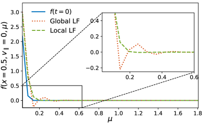
Figure 4: Relaxation of a 1X2V rectangular distribution with a coarse $\mu$-grid with $p=1$. Here we show the initial (solid blue) and final (dotted orange and dashed green) distribution functions after one collisional period. Dotted orange used global Lax-Friedrichs fluxes, dashed green used LF fluxes based on the local values at quadrature points.

4.4 Stability condition in the full gyrokinetic-GkLBO system

The (long wavelength) gyrokinetic system in (3)-(6) is also limited by the CFL constraints of the collisionless, or Hamiltonian, terms. We can estimate this condition by considering the kinetic equation

$$\frac{\partial f}{\partial t}+\nabla{{}_{\mbox{\boldmath$z$}}\cdot(\mbox{\boldmath$\alpha$}f})=0,$$ (80)

where the phase-space gradient $\nabla_{\mbox{\boldmath$z$}}\equiv\left(\nabla,\frac{\partial}{\partial v_{\parallel}}\right)$ acts on the flux $\mbox{\boldmath$\alpha$}f$ with a phase-space velocity $\mbox{\boldmath$\alpha$}\equiv(\dot{\mbox{\boldmath$R$}},\dot{v}_{\parallel})$. This is a nonlinear advection equation, for which we can use (71) to estimate the stability condition on each cell:

$$\lambda_{\mathcal{H}}=2\ C_{\mathrm{adv},p}\,(2p+1)\sum_{k}\frac{\max(0,\mbox{\boldmath$\alpha$}\cdot\hat{n}_{k})}{\Delta z_{k}},$$ (81)

where the $k$ sum is over all faces of the cell, $\hat{n}_{k}$ is the outward normal of the $k^{\rm{th}}$ face, and $\Delta z_{k}$ is the grid spacing in the direction corresponding to the $k^{\rm{th}}$ face. The form of the maximum function guarantees that the sum is only over faces where there is an outgoing flux. Although the eigenvalues of the full collisional gyrokinetic equation are not a sum of the collisionless eigenvalues and the GkLBO eigenvalues, we follow this conservative approach and compute the time step according to

$${\Delta}t\left(\lambda_{\mathcal{H}}+\lambda_{\mathrm{{GkLBO}}}\right)<\mathrm{CFL}.$$ (82)

An example of what establishes $\lambda_{\mathcal{H}}$ in the electrostatic limit is the electrostatic shear Alfvén or $\omega_{H}$ mode [34, 35]. A dispersion relation for this electrostatic instability can be derived by linearizing the collisionless form of (3) and (6). In the long-wavelength limit this becomes

$$\omega_{H}=\sqrt{\frac{n_{e}}{n_{0}}}\frac{|k_{\parallel}v_{te}|}{|k_{\perp}\rho_{s}|},$$ (83)

where $n_{0}$ is the linear ion polarization density used in the Poisson equation. We seek an estimate for $\mathrm{CFL}$ so that $\omega_{H,{\rm max}}{\Delta}t<1.73$, which is the stability limit for the RK3 time-stepping method. To estimate $\omega_{H,{\rm max}}$, assume $k_{\parallel,{\rm max}}\approx\Delta z=(2p+1)/\Delta z_{\mathrm{cell}}$ and $k_{\perp,{\rm min}}=\pi/L_{x}$, where $\Delta z$ is the cell spacing in $z$ and $L_{x}$ is the domain width in $x$. The initial time-step is set by the fastest parallel electron transit rate, $v_{\parallel,\max}$. The corresponding eigenvalue is $v_{\parallel,\max}/\Delta z=(2p+1)v_{\parallel,\max}/\Delta z_{\mathrm{cell}}$, giving a time-step estimate of

$$\Delta t=\frac{\Delta z_{\mathrm{cell}}\thinspace\mathrm{\mathrm{CFL}}}{(2p+1)v_{\parallel,\max}}.$$ (84)

Combining with (83) and the RK3 stability limit gives

$$\omega_{H,\max}{\Delta}t={\rm\mathrm{CFL}}\sqrt{\frac{n_{e,\max}}{n_{0}}}\frac{v_{te}\,L_{x}}{\pi v_{\parallel e,\max}\,\rho_{s}}<1.73,$$ (85)

which we use to set an appropriate value of $\mathrm{CFL}$ as an input parameter prior to run time. In the future, we plan to calculate $\omega_{H,\max}$ within the code to dynamically set the time-step limit due to the electrostatic shear Alvén mode.

5 Benchmark problems

In this section, we present tests designed to further understand the discrete scheme and to verify the accuracy of the gyrokinetic-GkLBO system. Relaxation tests without the collisionless terms demonstrate properties of the discrete GkLBO such as conservation, entropy and positivity. We also explore collisional Landau-damping to understand the physical implications of this model and compare it to analytic theory. Finally, simulations of 5D turbulence on helical, open field lines with collisions modeled by the GkLBO are presented.

5.1 Relaxation tests of the GkLBO

When an initial distribution function is subjected to the GkLBO alone, without the Hamiltonian terms, it will relax to the maximum entropy solution. In the continuous sense, the maximum entropy solution is the Maxwellian in (25), but the discrete equilibrium solution, $f_{Mh}$, is not necessarily the projection of (25) onto the DG basis. In principle, $f_{Mh}$ could be derived by repeating the derivation of (25) but assuming the discrete form of the GkLBO and a finite velocity domain. This implies that if we project $f_{M}$ onto the basis (e.g. using Gaussian quadrature) and use that as an initial condition, the system will not be static and will evolve some. Figure (5a), for example, shows this initial, projected Maxwellian and its final state after one collisional period. At first sight they are indistinguishable, but the difference, shown in figure (5b), shows that the projected Maxwellian was not in the kernel of the discrete $\mathcal{C}[f]$. These tests were carried out in a $[0,1]\times[-12v_{t},12v_{t}]$ domain with $2\times 96$ cells using a zero-drift Maxwellian with $v_{t}=1/\sqrt{2}$, $\nu=0.01$ and piecewise linear bases.

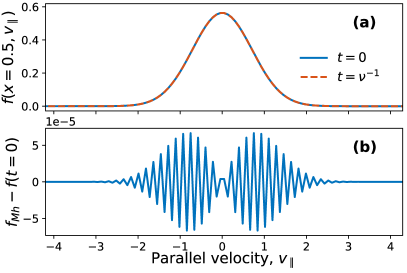
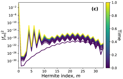
Figure 5: (a) An initial Maxwellian projected onto the DG basis and its final ($t=\nu^{-1}$) state after relaxation. (b) Difference between initial projection of the Maxwellian and final discrete equilibrium, i.e. $f_{Mh}=f(t=\nu^{-1})$. (c) Time evolution of the Hermite spectrum when initial state is a projected Maxwellian.

A Maxwellian is equivalent to the (properly normalized) Gaussian-weighted zeroth Hermite basis [36]. This is also an eigenfunction of $\mathcal{C}[f]$, as we will show in section 5.2. Therefore, in a continuous infinite velocity-space, its Hermite spectrum should remain a Dirac delta function peaked at the Hermite index $m=0$ as it is evolved in time according to (73). Ideally this ought to be reflected in the spectral analysis of the discrete data, but spectral transforms of DG data are subtle. If one transforms the data interpolated onto a finer grid (e.g. $\Delta x=\Delta x_{\mathrm{cell}}/(p+1)$ as in section 4) errors would be introduced in the higher modes due to the underlying piecewise discontinuous character. The appropriate way to transform DG data is by formulating it as a weak equivalence. Therefore the spectral transform of one-dimensional data onto a normalized Gaussian-weighted Hermite basis is given by

$$f_{\mathrm{DG}}(x)=\sum_{k=1}^{N_{p}}f_{k}\psi_{k}(x)\doteq f_{\mathrm{Hermite}}(x)=\sum_{m=0}^{m_{\mathrm{max}}}f_{m}\frac{1}{\sqrt{2^{m}m!}}\mathrm{H}_{m}(x)\frac{e^{-x^{2}}}{\sqrt{\pi}},$$ (86)

where $\mathrm{H}_{m}(x)$ is the $m$-th physicists’ Hermite polynomial. After projecting each of the Gaussian-weighted Hermite basis functions onto the DG basis using Gaussian quadrature, the weak equality in (86) yields a linear system of equations in the $f_{m}$ unknowns. When the number of DG degrees of freedom is larger than $m_{\mathrm{max}}+1$ this linear problem is solved via least squares. In multiple dimensions, one can project the function onto the the basis that excludes the to-be-transformed dimension, and perform a series of 1D transforms. Such operation was carried out with the projected Maxwellian subjected to (73), yielding the spectrum in figure (5c). This analysis suggests there exist contributions from modes other than $m=0$ at $t=0$ (darkest purple), albeit orders of magnitude smaller. As time proceeds all $m\neq 0$ modes grow, and high $m$ modes saturated at $\left|f_{m}\right|^{2}{\sim}10^{-18}$ form part the discrete maximum entropy solution.

The deviation of the spectrum in figure (5c) from the continuous, infinite space equivalent may be the result of a number of factors. The Gaussian-weighted Hermites are orthonormal in the infinite velocity space, but truncating the domain introduces errors in the orthonormality relation (i.e. the orthonormality integral no longer yields a Kronecker delta function). These errors should be small in the $[-12v_{t},12v_{t}]$ spaced used above. A greater difficulty in performing a Hermite spectral analysis arises from the discrete representation of the solution, and the Gaussian-weighted Hermites, in terms of discontinuous polynomial basis. The departure from orthonormality of the discrete Gaussian-weighted Hermites may be more significant than that of the continuous ones on a restricted domain. There is also some ambiguity as to how to project the Gaussian-weighted Hermites onto the DG basis; we used Gaussian quadrature, but one could also evaluate them at cell nodes to produce a continuous representation or use an exact projection. Additionally the least-squares solution of (86) may also introduces other errors, particularly if the corresponding matrix is ill-conditioned. Furthermore, notice that in figure (5c) the spectrum is truncated at $m_{\mathrm{max}}+1=34$. Initially we expected $m_{\mathrm{max}}+1$ to correspond to the number of modes whose roots are contained within our domain (44 in this case), but instead we found empirically that if $m_{\mathrm{max}}+1>34$ the Hermite analysis yields high $m$ mode amplitudes orders of magnitude larger. Further exploration of spectral transforms of DG data, including the a priori determination of $m_{\mathrm{max}}$, is an interesting enterprise currently ongoing in our group but which unfortunately is beyond the scope of this publication.

As we will show in section 5.2, the Hermite basis diagonalizes the GkLBO, turning (73) into

$$\frac{\partial f_{m}}{\partial t}=-\nu mf_{m}.$$ (87)

We can test the analytic solution to this equation, $f_{m}(t)=f_{m}(t=0)e^{-\nu mt}$, numerically by using $f_{m=0}=f_{m=5}=f_{m=10}=f_{m=20}=1$ and zero for all other modes, rather than only initializing $f_{m=0}=1$, as in figure (5). The time evolution of the three higher modes is shown in figure (6). Its agreement with analytic theory is very good in the $t\in[0,\nu^{-1}]$ time window, and if the discrete Hermite basis functions were eigenfunctions of our discrete GkLBO, the three higher modes would simply decay exponentially indefinitely. However, when the amplitude of the $m=20$ mode reaches the noise introduced by the evolution of $m=0$, the spectral analysis of $m=20$ begins to deviate from the analytic result. This noise we showed in figure (5c) is at a $\left|f_{m}\right|^{2}{\sim}10^{-18}$ level, and it is at that point that the green $m=20$ line in figure (6) deviates from its analytic expectation. Were this spectral analysis to be carried out with $m_{\mathrm{max}}+1<33$ the error in $m=20$ would be slightly larger at $\nu t>0.6$, but solving the least-squares problem in (86) with $m_{\mathrm{max}}+1>34$ yields errors orders of magnitude larger.

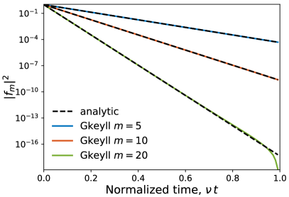
Figure 6: Time evolution of the (squared) Hermite expansion coefficients of the distribution function.

As the solution relaxes onto the discrete maximum entropy solution, $f_{Mh}$, it also exhibits a physical non-decreasing entropy. We again project the bump-on-tail distribution of (76) onto the in 1X2V $(x,v_{\parallel},\mu)$ DG basis, use a stable $\mathrm{CFL}=1$, and run to $\nu t=10$. The norm of the difference between $f(t)$ and the maximum entropy solution, $f_{Mh}=f(t=10\nu^{-1})$, decreases rapidly as shown in figure (7a). Meanwhile, the entropy, $S(t)=-\int f(t)\ln f(t)\thinspace\mathrm{d}x\thinspace\mathrm{d}^{3}\vv$, increases monotonically. The relative difference between initial entropy and $S(t)$ is given in figure (7b). Although we have not yet proven an $H$-theorem for the discrete operator (or proved its self-adjointness), the entropy is seen to increase in the cases we have explored. Part of the challenge in proving self-adjointness of the operator lies in guaranteeing that $f$ remains positive. Positivity of $f$ is something we are able to build into the discretization of the GkLBO’s drag term (not presented here), but additional work is needed to ensure the diffusion term does not cause $f$ to go negative.

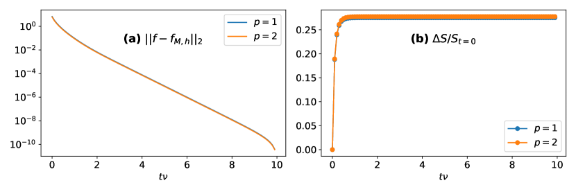
Figure 7: As a 1X2V a bump-on-tail distribution relaxes, the norm of the difference of $f$ and the discrete equilibrium solution $f_{Mh}=f(t=10\nu^{-1})$ decreases (a). The entropy $S$ increases monotonically, and so does the relative difference in $S$ (b).

These 1X2V relaxation tests also confirm the conservative properties of our scheme and, although not shown here, conservation of particle number, momentum, and energy are also guaranteed in higher dimensions. For the case of the 1X2V bump-on-tail initial condition, figure (8) shows the norm of the relative difference in the momentum and energy densities, $M_{1}$ and $M_{2}$. Over ten collisional periods the relative change in these quantities remains within machine precision, consistent with sections 3.2.2-3.2.4. In this case machine precision accuracy refers to the fact that the relative error per time step in the momentum is ${\sim}2{\times}10^{-12}/1400\sim 10^{-15}$, where 1400 is the approximate number of time steps. The non-vanishing boundary contributions in the surface term of (49) and in the calculation of the primitive moments, $u_{\parallel}$ and $v_{t}$, are necessary for exact conservation, even if $f$ is small at the boundaries. Neglecting these corrections gives errors in momentum and energy conservation that are orders of magnitude larger.

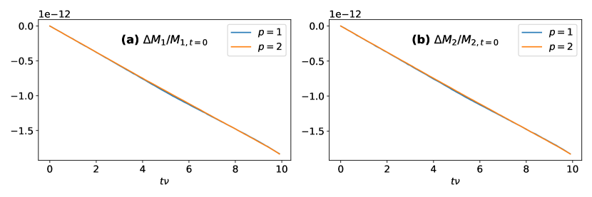
Figure 8: 1X2V relaxation of a bump-on-tail distribution with $p=1$ and $p=2$. Relative norm of the difference in (a) momentum density $M_{1}$ and (b) energy density $M_{2}$, as a function of time. Both are conserved to machine precision.

5.2 Collisional Landau damping of ion acoustic waves

The study of collisionless (Landau) damping of plasma waves due to velocity-space resonance dates back to the origins of plasma physics, and its modification due to the presence of collisions remains an important area of research. Ion sound waves suffer from this decay, and scientists have been constructing a theory of such phenomenon for decades. Consider that neutral sound waves are undamped in its highly (molecular) collisionality environment, so one may expect that as collisions become more frequent Landau damping of ion acoustic waves would weaken. The consensus, however, is that the actual trend depends on whether one considers self-species collisions, multi-species collisions, or both. The description of collisional Landau damping can also vary with the collision operator employed. An early study with a Krook operator [37] noted that under ion-ion collisions alone the damping rate ($\gamma=-\mathrm{Im}\thinspace\omega$) monotonically decreases towards the regular sound wave limit ($\gamma\to 0$) as as $\nu_{ii}$ increases if the temperature ratio $\tau=T_{i}/T_{e}=1$. This was not limited to the simple Krook operator as numerical integration of the Vlasov-FPO equation also arrived at the same conclusion [38]. But these studies, and also [39], quickly noticed that in non-equilibrium cases of nonequal temperatures, specifically $\tau<1$, the damping rate can first undergo a period of growth before starting to decrease towards the undamped fluid limit. Even at equal temperatures, including electron-ion collisions can increase the damping rate [40].

Landau damping of plasma sound waves is central to ion-temperature gradient instabilities, ion acoustic instabilities and other transport processes in astrophysical and laboratory plasmas. As a commonplace ingredient in plasmas, it is not only necessary to understand its collisional modifications with the full FPO, but also with the simple models frequently used by analytic and computational studies. The model-FPO Dougherty operator considered here has been explored little in the context of ion-acoustic waves. One of the few studies available [41] explored ion-acoustic instabilities in the presence of self-species and multi-species collisions, and was only able to do so at low collisionalities (i.e. $(\nu_{ee}+\nu_{ie})/(k_{\parallel}v_{te})\ll 1$). The study of collisional Landau damping of ion-acoustic waves at arbitrary collisionality here then serves as both documentation of this process with the Dougherty operator, and also as validation of our scheme and implementation within Gkeyll.

Consider a system consisting of a single-ion hydrogen plasma in a curvature-free homogeneous magnetic field such that $\mathcal{J}=B=\mbox{\boldmath$b$}\cdot\mbox{\boldmath$B$}=\mathbf{\hat{z}}\cdot\mbox{\boldmath$B$}$. The electrons will be assumed adiabatic and will not collide with the ions (only ion self-species collisions are included here), so we refer to the collisionality $\nu_{ii}=\nu$. Then one only needs to evolve the ion equation (3), which upon linearization about an equilibrium, $f=f_{0}+f_{1}$ (we omit the ion subscript here for simplicity), simply becomes

$$\frac{\partial f_{1}}{\partial t}+v_{\parallel}\frac{\partial f_{1}}{\partial z}+\frac{1}{B}\left[\phi,f_{0}\right]-\frac{e}{m}\frac{\partial\phi}{\partial z}\frac{\partial f_{0}}{\partial v_{\parallel}} =C[f_{0},f_{1}]$$ (88)

$$=\nu\left\{\frac{\partial}{\partial v_{\parallel}}\left[\left(v_{\parallel}-u_{\parallel,0}\right)f_{1}-u_{\parallel,1}f_{0}+v_{t,0}^{2}\frac{\partial f_{1}}{\partial v_{\parallel}}+v_{t,1}^{2}\frac{\partial f_{0}}{\partial v_{\parallel}}\right]\right.$$

$$\left.\qquad+\frac{\partial}{\partial\mu}2\mu\left[f_{1}+\frac{m}{B}\left(v_{t,0}^{2}\frac{\partial f_{1}}{\partial\mu}+v_{t,1}^{2}\frac{\partial f_{0}}{\partial\mu}\right)\right]\right\}.$$

The simplified Poisson bracket $[F,G]=\mbox{\boldmath$b$}\cdot\nabla F\times\nabla G$ vanishes since $f_{0}$ is homogeneous in configuration space, and the first-order primitive moments are defined as

$$u_{\parallel,1} =\frac{2\pi B}{mn_{0}}\int v_{\parallel}f_{1}\thinspace\thinspace\mathrm{d}v_{\parallel}\thinspace\mathrm{d}\mu,$$ (89)

$$v_{t,1}^{2} =\frac{2\pi B}{3mn_{0}}\int\left(\frac{2\mu B}{m}+v_{\parallel}^{2}-3v_{t,0}^{2}\right)f_{1}\thinspace\thinspace\mathrm{d}v_{\parallel}\thinspace\mathrm{d}\mu,$$ (90)

and $n_{0}$, $u_{\parallel,0}$ and $v_{t,0}$ are the number density, mean velocity and thermal speed of $f_{0}$, respectively, although we have assumed $u_{\parallel,0}=0$. It is convenient to write the perturbed distribution as $f_{1}=f_{0}\varphi$ with $\varphi\ll 1$. The linearized collision operator then becomes

$$C[f_{0},f_{1}]=\nu f_{0} \left\{-\left(v_{\parallel}-u_{\parallel,0}\right)\frac{\partial\varphi}{\partial v_{\parallel}}+v_{t,0}^{2}\frac{\partial^{2}\varphi}{\partial v_{\parallel}^{2}}-2\mu\frac{\partial\varphi}{\partial\mu}+\frac{mv_{t,0}^{2}}{B}\frac{\partial}{\partial\mu}2\mu\frac{\partial\varphi}{\partial\mu}\right.$$ (91)

$$\left.\quad-\frac{v_{t,1}^{2}}{v_{t,0}^{2}}\left[3-\frac{2\mu B}{mv_{t,0}^{2}}-\frac{\left(v_{\parallel}-u_{\parallel,0}\right)^{2}}{v_{t,0}^{2}}\right]+u_{\parallel,1}\frac{v_{\parallel}-u_{\parallel,0}}{v_{t,0}^{2}}\right\}.$$

We have assumed there is no equilibrium component to the electrostatic potential ($\phi=\phi_{1}$), and from here on we will make use of the normalized variables $2\mu B/(mv_{t,0}^{2})\to\mu$ and $v_{\parallel}/v_{t,0}\to v_{\parallel}$. Assuming wave-like modes according to the ansatz $f_{1}=\hat{f}\exp[i(kz-\omega t)]$, $\phi=\hat{\phi}\exp[i(kz-\omega t)]$, and employing the quasineutrality between adiabatic electrons and the equilibrium ion distribution (via Poisson’s equation), renders our kinetic equation into

$$i\left(v_{\parallel}-\Omega\right)\hat{f}+i\pi v_{t,0}^{3}v_{\parallel}\frac{f_{0}}{n_{0}}\frac{T_{e0}}{T_{i0}}\int\hat{f}\thinspace\thinspace\mathrm{d}v_{\parallel}\thinspace\mathrm{d}\mu-\eta f_{0}\chi\left(\varphi\right)=0.$$ (92)

We now refer to the normalized mode frequency, $\Omega=\omega/(k_{\parallel}v_{t,0})$, and the normalized collisionality $\eta=\nu/(k_{\parallel}v_{t,0})$, and $\chi(\varphi)$ is the term between curly brackets in (91).

One can proceed by expanding in a set of Hermite-Laguerre polynomials [42] as

$$\varphi=\sum_{m,n=0}^{\infty}a_{mn}\varphi_{mn}=\sum_{m,n=0}^{\infty}a_{mn}\frac{1}{\sqrt{m!}}\mathrm{He}_{m}\left(v_{\parallel}\right)L_{n}\left(\mu/2\right),$$ (93)

which satisfy the orthogonality relation

$${\left\langle\varphi_{nn^{\prime}},\varphi_{mm^{\prime}}\right\rangle}=\frac{1}{2\sqrt{2\pi}}\int\varphi_{nn^{\prime}}\varphi_{mm^{\prime}}e^{-(v_{\parallel}^{2}+\mu)/2}\thinspace\thinspace\mathrm{d}v_{\parallel}\thinspace\mathrm{d}\mu=\delta_{n,m}\delta_{n^{\prime},m^{\prime}}.$$ (94)

Together with the recursion relations

$$\mathrm{He}_{m+1}(v_{\parallel}) =v_{\parallel}\mathrm{He}_{m}(v_{\parallel})-m\mathrm{He}_{m-1}(v_{\parallel}),$$ (95)

$$(\mu/2)L_{n}^{\prime}(\mu/2) =nL_{n}(\mu/2)-nL_{n-1}(\mu/2)$$

one may find the projection of the transformed linear kinetic equation 92 onto the basis $\varphi_{mn}$. This projection, after some algebra, is

$${\left\langle\varphi_{mn},\mathrm{Eq.~{}\ref{eq:linKinEq}}\right\rangle}=\begin{cases}\Omega a_{10}-a_{00}-\sqrt{2}a_{20}-\frac{T_{e0}}{T_{i0}}a_{00}=0\qquad(m,n)=(1,0)\\ \Omega a_{20}-\sqrt{2}a_{10}-\sqrt{3}a_{30}+i\eta\left(\frac{4}{3}a_{20}+\frac{2\sqrt{2}}{3}a_{01}\right)=0\qquad(m,n)=(2,0)\\ \Omega a_{01}-a_{11}+i\eta\left(\frac{2}{3}a_{01}+\frac{2\sqrt{2}}{3}a_{20}\right)=0\qquad(m,n)=(0,1)\\ \left[\Omega+i\eta(m+2n)\right]a_{mn}-\sqrt{m}a_{(m-1)n}-\sqrt{m+1}a_{(m+1)n}=0\qquad\mathrm{all~{}other}~{}(m,n).\end{cases}$$ (96)

From the last of these equations one can show that for a physically realizable solution $a_{(m+1)n}/a_{mn}\to a_{mn}/i\eta\sqrt{m}$ as $m\to\infty$ [43]. The presence of collisions limits the extent of the spectrum in $m$, allowing us to truncate the expansion at an upper limit $m_{\mathrm{max}}$. One can then use

$$\left[\Omega+i\eta\left(m_{\mathrm{max}}+2n\right)\right]a_{m_{\mathrm{max}}n}-\sqrt{m_{\mathrm{max}}}a_{(m_{\mathrm{max}}-1)n}=0$$ (97)

in conjunction with the last relation in (96) to iterate backwards from $m_{\mathrm{max}}$ and find:

$$a_{m0}=\cfrac{\sqrt{m}}{\Omega+i\eta m-\cfrac{m+1}{\Omega+i\eta\left(m+1\right)-\cfrac{m+2}{\Omega+i\eta(m+2)-\dots\cfrac{m_{\mathrm{max}}}{\Omega+i\eta m_{\mathrm{max}}}}}}a_{(m-1)0}.$$ (98)

A similar relation is obtained for $n=1$. Since the recursion relation in (96) does not couple Laguerre moments together, one need only solve the system for $a_{00}$, $a_{10}$, $a_{20}$ and $a_{01}$. The coefficients $a_{30}$ and $a_{11}$ can be written in terms of continued fractions like (98), and one obtains a linear problem with the determinant of the mass matrix yielding the dispersion relation [42]

$$\frac{T_{i0}}{T_{e0}}=\frac{8\eta^{2}+9F_{1}F_{2}}{8\eta^{2}\left(\Omega^{2}-1\right)+9\left[\left(\Omega^{2}-1\right)F_{1}-2\Omega\right]F_{2}},$$ (99)

where the functions $F_{1}(\Omega,\eta)$ and $F_{2}(\Omega,\eta)$ are

$$F_{1}\left(\Omega,\eta\right) =\Omega+\cfrac{4}{3}i\eta-\cfrac{3}{\Omega+3i\eta-\cfrac{4}{\Omega+4i\eta-\cfrac{5}{\Omega+5i\eta-\dots\cfrac{m_{\mathrm{max}}}{\Omega+i\eta m_{\mathrm{max}}}}}},$$ (100)

$$F_{2}\left(\Omega,\eta\right) =\Omega+\cfrac{2}{3}i\eta-\cfrac{1}{\Omega+3i\eta-\cfrac{2}{\Omega+4i\eta-\cfrac{3}{\Omega+5i\eta-\dotsc\frac{m_{\mathrm{max}}}{\Omega+i\eta\left(m_{\mathrm{max}}+2\right)}}}}.$$

We set up an analogous scenario in Gkeyll using adiabatic electrons, $\tau=1.0$, hydrogen mass ratio and perturbed the initial state using a wave mode with $k_{\parallel}\rho_{i}=0.5$. These simulations were done on a domain $[-\pi/k_{\parallel},\pi/k_{\parallel}]\times[-6v_{ti},6v_{ti}]\times[0,m_{i}(5v_{ti})^{2}/(2B)]$ discretized with $64\times 128\times 16$ cells. This resolution and the time step stability constraints are probably conservative and were chosen to guarantee these results were well converged. In figure (9a) the decay of the wave is displayed by the decrease in electrostatic energy over time, from which one can measure both the real part and the imaginary part of the wave frequency. The energy trace of three different collisionalities show that as ion-ion collisions alone become more frequent, the damping mechanism is progressively eroded. We scanned the entire collisional range and compared our results to the roots of the dispersion relation in (99). Figure (9b) shows excellent agreement between theory and our implementation in Gkeyll. Consistent with intuition, when the mean-free-path becomes comparable to the wavelength, $\nu/(k_{\parallel}v_{ti})\sim 1$, fewer particles will be able to resonate with the wave before experiencing collisional scattering, thus considerably reducing damping. In the high-frequency limit, collisions maintain the plasma in a local thermodynamic equilibrium so the plasma behaves like an ideal gas that has undamped compressional oscillations. This test also confirms an earlier partial agreement between theory and simulation of Landau damping of electron (Langmuir) waves due to a disparity in the dimensionality of the two [22].

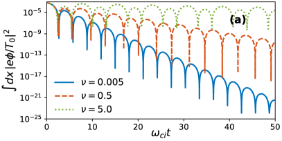
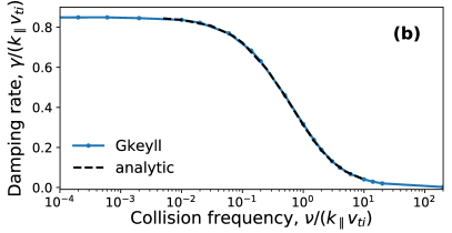
Figure 9: (a) Field energy time trace and (b) damping rates as a function of collisionality for the ion acoustic wave.

5.3 Helical open-field-line plasma turbulence

We now present a benchmark test of the full 5D (long-wavelength) gyrokinetic system, given by (3)-(6). With the moment-conserving GkLBO, we simulated plasma turbulence on helical, open field lines, using a nonorthogonal field-line-following coordinate system as in [44, 45]. In this coordinate system, $z$ is parallel to magnetic field lines, $x$ is the radial coordinate, and $y$ is the “bi-normal” coordinate. To ensure numerical stability, we used (85) to determine that $\mathrm{CFL}$ $\approx 0.28$ was necessary to prevent the electrostatic shear Alfén mode from becoming unstable. We set $\mathrm{CFL}$ $=0.2$ as a conservative estimate. We used the same physical parameters as in [45] to simulate the Texas Helimak simple magnetized torus experiment and make direct comparison with those results. We calculated the ion and electron collision frequencies from [46] using background densities ($n_{0}$) and temperatures ($T_{s0}$) that are constant in space and time. It is important to note that simulations in [45] included collision frequencies with spatially- and time-varying densities and temperatures, as well as electron-ion collisions (but no ion-electron collisions). Those simulations were also carried out with an earlier, nodal DG scheme employing different algorithms than those presented here while still remaining conservative by correcting for the errors. We denote this by $\nu_{ss^{\prime}}(\mathbf{x},t)$ to differentiate it from simulations presented here with the moment-conserving GkLBO, using the constant collision frequency $\nu_{s}$ and neglecting multi-species collisions. We also present results from a simulation with a reduced collision frequency, $0.1\nu_{s}$. All simulations were run to 16 ms. Calculated equilibrium profiles were averaged in time from 10 to 16 ms and in the bi-normal direction $y$.

Figure (10) shows snapshots of electron density, electron temperature, and plasma potential in the nonorthogonal field-line-following coordinate system at 10 ms. Turbulent structures and density levels are very similar to those presented in [45], though electron temperature and plasma potential values are slightly greater. Electron density profiles are compared in figure (11a), with all three profiles being very similar. More differences are visible in figure (11b), which compares the electron temperature profiles. Compared to the simulation with constant like-species collisionality only (dotted blue line in figure (11b)), including electron-ion collisions and spatially varying collisionality (solid green line figure (11b)) reduced the electron temperature. Given the inverse dependence of the interchange linear growth rate on the electron-ion collisionality [47] one may consider the possibility of cross-field transport increasing as $\nu_{ei}$ decreases; were this effect to be significant parallel transport would be less competitive against perpendicular fluxes and would not carry out heat through the sheath as efficiently, leading to a temperature increase across the plasma. However the linear analysis suggests that the interchange growth rate is only weakly dependent on $\nu_{ei}$ [47]. Instead, a contributing factor to the increase of $T_{e}$ when collisions strengthen is that due to pitch-angle scattering more electrons are carried to higher $v_{\parallel}$, where they are lost through the sheath. This effect can increase the heat loss rate, lowering the temperature of the remaining electrons. Such mechanism would also apply to the increase in $T_{e}$ seen in comparing the simulation using constant like-species collisions (dotted blue line in figure (11b)) with a similar simulation which used a reduced collisionality (orange dash-dot line in figure (11b)).

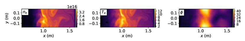
Figure 10: Snapshots of electron density (left), electron temperature (middle), and plasma potential (right) in the $xy$-plane, from simulations of plasma turbulence on helical, open field lines in 5D with the moment-conserving GkLBO.

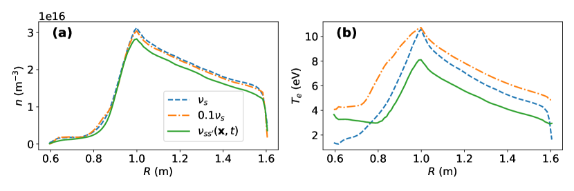
Figure 11: Comparison of (a) electron density and (b) electron temperature equilibrium profiles from simulations with different constant collision frequencies ($\nu_{s},0.1\nu_{s}$) to that with time- and spatially-varying collision frequencies and multi-species collisions ($\nu_{ss^{\prime}}(\mbox{\boldmath$x$},t)$).

Plasma potential profiles are compared in figure (12a). All three $\phi(R)$ profiles are relatively similar, and any collisionality-induced changes to the $E{\times}B$ profile do not appear significant enough to indicate that shear stabilization would play a major role in the changes to the simulated profiles or the turbulence. It is however interesting that the constant like-species collisionality simulation with higher $T_{e}$ (orange dash-dot line in figure (11b)) is actually the one with a lower potential, contrary to what we would expect from an adiabatic electron response $e\phi\sim\Lambda T_{e}$. One possibility is possible that the lower collisionality allows for an increasingly non-adiabatic response of the plasma potential. It is also possible that despite the increase in $T_{e}$ there is a stronger decrease in $\Lambda$: at low collisionality fewer electrons scatter above the sheath potential, so the sheath potential has to drop to allow more electrons to escape in order to match the ion flux into the sheath. Lastly, we highlight that density fluctuation levels are reduced for the lower collision frequency case as compared with the other simulations (figure (12b)).

A more in depth analysis of the physics of these simulations is possible but beyond the scope of this manuscript. In general the intention here is to demonstrate that the moment-conserving GkLBO presented in this work has been successfully incorporated into more complex 5D simulations, and that despite being limited to like-species collisions it produces results with reasonable agreement with previous simulations [45]. This agreement will likely improve by including features such as spatially-varying collision frequencies and multi-species collisions.

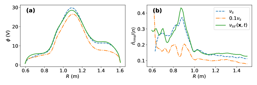
Figure 12: Comparison of (a) plasma potential and (b) density fluctuation profiles from simulations with different constant collision frequencies ($\nu_{s},0.1\nu_{s}$) to that with time- and spatially-varying collision frequencies and multi-species collisions. A non-adiabatic electron response might explain the slight decrease in the plasma potential in the lower collisionality case. Turbulence levels in (b) are also reduced for the lower collisionality case.

6 Discussion and summary

We have presented a gyroaveraged Lenard-Bernstein-Dougherty collision operator (GkLBO), including a novel formulation of the discrete discontinuous Galerkin form and its implementation in Gkeyll. Building upon [22], we use the concept of weak equality to formulate a recovery DG (RDG) algorithm for the diffusion term of the GkLBO. It also provides a rigorous means to compute the primitive moments, $u_{\parallel}$ and $v_{t}$. If such calculations are carried out using point-wise or cell average-based operations, significant errors ensue, causing non-conservation and instability. This concept guarantees that our discrete operator retains conservation properties and leads to an energy-conserving scheme even in the case of piecewise linear basis functions, provided that we carefully consider quadratic quantities projected onto the $p=1$ basis. Weak equality is also crucial in the definition of spectral transforms of DG data.

The continuous GkLBO is self-adjoint and satisfies the $H$-theorem but we have not yet proven that the discrete operator retains such properties. This is challenging because the present discrete operator does not guarantee $f>0$, though we have already implemented a positivity-preserving drag term (not presented here). Self-adjointness enhances the efficacy of some approaches to accelerate the time integration (e.g. super time-stepping [32]), which we eventually wish to implement in order to more efficiently model highly collisional plasmas. Guaranteeing positivity, self-adjointness and non-decreasing entropy in the DG discretization scheme is the objective of on-going work.

We analyzed the stability conditions for DG advection and diffusion problems, and used this to establish the time step stability criterion for the GkLBO. Satisfying these conditions helps to avoid some issues associated with negative values of the distribution function, since $f>0$ is not currently guaranteed in our scheme. For the SSP-RK3 time integration in Gkeyll, we presented a conservative estimate of the largest, stable time step.

Relaxation tests of the pure GkLBO demonstrated the exact numerical conservation properties of our scheme. These systems evolved to a maximum entropy solution which, as shown through a Hermite spectral lens, is subtly different from a Maxwellian projected onto the DG basis. This makes the Hermite analysis of collisional DG data more complicated for the larger Hermite moments, since the high-$m$ noise associated with the evolution of the zeroth-order Hermite moment causes higher moments to deviate from the analytic solution. However, lower moments of the GkLBO evolve according to analytic theory, and the evolution of higher moments converges with resolution.

We performed tests of collisional Landau damping of ion acoustic waves. Using a Hermite-Laguerre basis, we obtained a dispersion relation whose least-damped roots agreed well with simulation results. We presented a more complicated test of 5D turbulence on open, helical field lines in the Texas Helimak device, which agreed well with previous simulations, even without the additional physics of multi-species collisions and spatially-varying collision frequencies. Multi-species collisions give rise to slightly different (discrete) conservation laws and requirements for the calculation of the velocities and thermal speeds in the cross-collision terms. More accurate gyrokinetic simulations of laboratory and astrophysical plasmas will include spatially-varying, and even velocity-dependent, collisionalities. These features are currently being developed and tested within the Gkeyll code.

Appendix A Accessing and running Gkeyll

The Gkeyll code (in binary and source format) and the input files to reproduce results presented here are available for download. Gkeyll installation instructions can be found on the Gkeyll website (http://gkeyll.readthedocs.io). The code can be installed on Unix-like operating systems (including Mac OS and Windows using the Windows Subsystem for Linux) either by installing the pre-built binaries using the conda package manager or building the code via sources. The input files for simulations presented here can be found at https://github.com/ammarhakim/gkyl-paper-inp/tree/master/GkLBO.

References

References

- [1] M. N. Rosenbluth, W. M. MacDonald, D. L. Judd, Fokker-planck equation for an inverse-square force, Phys. Rev. 107 (1) (1957) 1–6. doi:10.1103/PhysRev.107.1.
- [2] H. Sugama, Gyrokinetic field theory, Physics of Plasmas 7 (2) (2000) 466–480. doi:10.1063/1.873832.
- [3] A. J. Brizard, T. S. Hahm, Foundations of nonlinear gyrokinetic theory, Rev. Mod. Phys. 79 (2007) 421–468. doi:10.1103/RevModPhys.79.421.
- [4] J. A. Krommes, The gyrokinetic description of microturbulence in magnetized plasmas, Annual Review of Fluid Mechanics 44 (1) (2012) 175–201. doi:10.1146/annurev-fluid-120710-101223.
- [5] N. R. Mandell, A. Hakim, G. W. Hammett, M. Francisquez, Electromagnetic full- gyrokinetics in the tokamak edge with discontinuous Galerkin methods (2019). arXiv:arXiv:1908.05653.
- [6] M. G. McCoy, A. A. Mirin, J. Killeen, FPPAC: A two-dimensional multispecies nonlinear Fokker-Planck package, Computer Physics Communications 24 (1) (1981) 37–61.
- [7] J. Killeen, G. Kerbel, M. McCoy, A. Mirin, Computational methods for kinetic models of magnetically confined plasmas, Springer-Verlag, 1986.
- [8] R. Harvey, M. McCoy, The CQL3D Fokker-Planck Code, in: Proc. of IAEA Technical Committee Meeting on Advances in Simulation and Modeling of Thermonuclear Plasmas, Montreal, 1992, pp. 489–526, http://www.compxco.com/cql3d.html.
- [9] M. A. Dorf, R. H. Cohen, M. Dorr, J. Hittinger, T. D. Rognlien, Progress with the COGENT Edge Kinetic Code: Implementing the Fokker-Planck Collision Operator, Contributions to Plasma Physics 54 (4‐6) (2014) 517–523. doi:10.1002/ctpp.201410023.
- [10] R. Hager, E. S. Yoon, S. Ku, E. F. D. Azevedo, P. H. Worley, C. S. Chang, A fully non-linear multi-species Fokker-Planck-Landau collision operator for simulation of fusion plasma, J. Comput. Phys. 315 (2016) 644–660. doi:10.1016/j.jcp.2016.03.064.
- [11] P. J. Catto, K. T. Tsang, Linearized gyro‐kinetic equation with collisions, The Physics of Fluids 20 (3) (1977) 396–401. doi:10.1063/1.861902.
- [12] I. G. Abel, M. Barnes, S. C. Cowley, W. Dorland, A. A. Schekochihin, Linearized model Fokker-Planck collision operators for gyrokinetic simulations. I. Theory, Physics of Plasmas 15 (12) (2008) 122509. doi:10.1063/1.3046067.
- [13] P. J. Catto, D. R. Ernst, Alternate form of model like particle collision operator, Plasma Phys. Control. Fusion 51 (2009) 062001. doi:10.1088/0741-3335/51/6/062001.
- [14] H. Sugama, T. H. Watanabe, M. Nunami, Linearized model collision operators for multiple ion species plasmas and gyrokinetic entropy balance equations, Phys. Plasmas 16 (11) (2009) 112503. doi:10.1063/1.3257907.
- [15] D. Esteve, X. Garbet, Y. Sarazin, V. Grandgirard, T. Cartier-Michaud, G. Dif-Pradalier, P. Ghendrih, G. Latu, C. Norscini, A multi-species collisional operator for full-F gyrokinetics, Phys. Plasmas 22 (December) (2015) 122506. doi:10.1063/1.4937373.
- [16] H. Sugama, S. Matsuoka, S. Satake, M. Nunami, T. Watanabe, Improved linearized model collision operator for the highly collisional regime (2019). arXiv:arXiv:1906.07427.
- [17] P. Donnel, X. Garbet, Y. Sarazin, V. Grandgirard, Y. Asahi, N. Bouzat, E. Caschera, A multi-species collisional operator for full-F global gyrokinetics codes : Numerical aspects and verification with the GYSELA code, Comput. Phys. Commun. 234 (2019) 1–13. doi:10.1016/j.cpc.2018.08.008.
- [18] B. Li, D. R. Ernst, Gyrokinetic fokker-planck collision operator, Phys. Rev. Lett. 106 (19) (2011) 1–4.
- [19] Q. Pan, D. R. Ernst, Gyrokinetic Landau collision operator in conservative form, Phys. Rev. E 99 (November 2018) (2019) 023201. doi:10.1103/PhysRevE.99.023201.
- [20] Q. Pan, D. R. Ernst, P. Crandall, First Implementation of Gyrokinetic Exact Linearized Landau Collision Operator and Comparison with Models, Accepted for publication in Phys. Plasmas, April, 2020.
- [21] R. Jorge, B. J. Frei, P. Ricci, Non-Linear Gyrokinetic Coulomb Collision Operator (2019). arXiv:arXiv:1906.03252.
- [22] A. Hakim, M. Francisquez, J. Juno, G. W. Hammett, Conservative Discontinuous Galerkin Schemes for Nonlinear Fokker-Planck Collision Operators (2019). arXiv:arXiv:1903.08062.
- [23] E. Shi, G. Hammett, T. Stoltzfus-Dueck, A. Hakim, Gyrokinetic continuum simulation of turbulence in a straight open-field-line plasma, J. Plasma Phys. 83 (3) (2017) 905830304. doi:10.1017/S002237781700037X.
- [24] A. Hakim, G. W. Hammett, E. L. Shi, N. R. Mandell, Discontinuous Galerkin schemes for a class of Hamiltonian evolution equations with applications to plasma fluid and kinetic problems, SIAM J. Sci. Comput. (submitted) (2019) arXiv:1908.01814.
- [25] J. P. Dougherty, Model Fokker-Planck Equation for a Plasma and Its Solution, Phys. Fluids 7 (11) (1964) 1788–1799. doi:10.1063/1.2746779.
- [26] D. N. Arnold, G. Awanou, The Serendipity Family of Finite Elements, Foundations of Computational Mathematics 11 (3) (2011) 337–344.
- [27] S. Brenner, L. Scott, The Mathematical Theory of Finite Element Methods, Texts in Applied Mathematics, Springer New York, 2002.
- [28] B. van Leer, S. Nomura, Discontinuous Galerkin for Diffusion, in: 17th AIAA Comput. Fluid Dyn. Conf., no. AIAA 2005-5109, American Institute of Aeronautics, Toronto, Ontario, Canada, 2005. doi:10.2514/6.2005-5108.
- [29] B. Cockburn, C. Shu, The Local Discontinuous Galerkin Method for Time-Dependent Convection-Diffusion Systems, SIAM Journal on Numerical Analysis 35 (6) (1998) 2440–2463. doi:10.1137/S0036142997316712.
- [30] A. H. Hakim, G. W. Hammett, E. L. Shi, On discontinuous Galerkin discretizations of second-order derivatives (2014). arXiv:1405.5907.
- [31] D. Durran, Numerical Methods for Fluid Dynamics: With Applications to Geophysics, Texts in Applied Mathematics, Springer New York, 2010.
- [32] C. D. Meyer, D. S. Balsara, T. D. Aslam, A stabilized Runge-Kutta-Legendre method for explicit super-time-stepping of parabolic and mixed equations, Journal of Computational Physics 257 (2014) 594 – 626. doi:10.1016/j.jcp.2013.08.021.
-
[33]
B. Cockburn, C.-W. Shu,
Runge–Kutta Discontinuous
Galerkin Methods for Convection-Dominated Problems, Journal of Scientific
Computing 16 (3) (2001) 173–261.
doi:10.1023/A:1012873910884.
URL https://doi.org/10.1023/A:1012873910884 - [34] E. A. Belli, G. W. Hammett, A numerical instability in an ADI algorithm for gyrokinetics, Comput. Phys. Commun. 172 (2005) 119–132. doi:10.1016/j.cpc.2005.06.007.
- [35] E. L. Shi, Gyrokinetic Continuum Simulation of Turbulence in Open-Field-Line Plasmas, Ph.D. thesis, Princeton University (2017). arXiv:1708.07283, doi:10.1017/S002237781700037X.
- [36] T. Adkins, A. A. Schekochihin, A solvable model of Vlasov-kinetic plasma turbulence in Fourier-Hermite phase space, J. Plasma Phys. 84 (2018) 905840107. doi:10.1017/S0022377818000089.
- [37] D. Bhadra, R. K. Varma, Collisional Damping of Ion Waves in a Plasma, Phys. Fluids 7 (1964) 1091. doi:10.1063/1.1711334.
- [38] M. Ono, R. M. Kulsrud, Frequency and damping of ion acoustic waves, Phys. Fluids 18 (10) (1975) 1287. doi:10.1063/1.861016.
- [39] C. J. Randall, Effect of ion collisionality on ion-acoustic waves, Phys. Fluids 25 (12) (1982) 2231. doi:10.1063/1.863963.
- [40] E. M. Epperlein, R. W. Short, A. Simon, Damping of ion-acoustic waves in the presence of electron-ion collisions, Phys. Rev. Lett. 69 (1992) 1765–1768. doi:10.1103/PhysRevLett.69.1765.
- [41] B. R. S. B. Ong, M. Y. Yu, The effect of weak collisions on ion-acoustic wave instabilities in a current-carrying plasma, J. Plasma Phys. 3 (3) (1969) 425–433. doi:10.1017/S0022377800004505.
- [42] M. W. Anderson, T. M. O’Neil, Collisional damping of plasma waves on a pure electron plasma column, Physics of Plasmas 14 (11) (2007) 112110. doi:10.1063/1.2807220.
- [43] C. S. Ng, A. Bhattacharjee, F. Skiff, Kinetic eigenmodes and discrete spectrum of plasma oscillations in a weakly collisional plasma, Phys. Rev. Lett. 83 (1999) 1974–1977. doi:10.1103/PhysRevLett.83.1974.
- [44] E. L. Shi, G. W. Hammett, T. Stoltzfus-Dueck, A. Hakim, Full- gyrokinetic simulation of turbulence in a helical open-field-line plasma, Physics of Plasmas 26 (1) (2019) 012307. doi:10.1063/1.5074179.
- [45] T. N. Bernard, E. L. Shi, K. W. Gentle, A. Hakim, G. W. Hammett, T. Stoltzfus-Dueck, E. I. Taylor, Gyrokinetic continuum simulations of plasma turbulence in the texas helimak, Physics of Plasmas 26 (4) (2019) 042301. doi:10.1063/1.5085457.
- [46] J. Huba, NRL Plasma Formulary 2009, Tech. rep., Naval Research Lab, Beam Physics Branch, Washington, DC (2009).
- [47] P. Ricci, B. N. Rogers, Three-dimensional fluid simulations of a simple magnetized toroidal plasma, Physics of Plasmas 16 (9) (2009) 092307. doi:10.1063/1.3230119.