Choked accretion onto a Kerr black hole

Abstract

The choked accretion model consists of a purely hydrodynamical mechanism in which, by setting an equatorial to polar density contrast, a spherically symmetric accretion flow transitions to an inflow-outflow configuration. This scenario has been studied in the case of a (non-rotating) Schwarzschild black hole as central accretor, as well as in the non-relativistic limit. In this article, we generalize these previous works by studying the accretion of a perfect fluid onto a (rotating) Kerr black hole. We first describe the mechanism by using a steady-state, irrotational analytic solution of an ultrarelativistic perfect fluid, obeying a stiff equation of state. We then use hydrodynamical numerical simulations in order to explore a more general equation of state. Analyzing the effects of the black hole’s rotation on the flow, we find in particular that the choked accretion inflow-outflow morphology prevails for all possible values of the black hole’s spin parameter, showing the robustness of the model.

I Introduction

Black hole accretion theory has been an important building-block of our current understanding of high-energy astrophysical phenomena such as X-ray Binaries, Gamma Ray Bursts, and Active Galactic Nuclei mAcF2013 . In recent years, this field of knowledge has gone through a revolution led by the observational breakthrough of gravitational wave astronomy, that has allowed a systematic analysis of close to fifty binary black hole mergers to date ligo2019 ; ligo2020 , as well as the extreme-resolution imaging of the immediate environment of astrophysical black holes achieved by the Event Horizon Telescope EHT_M87 .

Since the pioneering work of Bondi hB52 , the introduction of exact, analytic solutions for modeling different astrophysical scenarios has been instrumental in the continuous development of accretion theory. Analytic models, by transparently highlighting the role played by different physical ingredients, are key in cementing our understanding and building our intuition around the studied phenomena. Moreover, analytic solutions are crucial tools as benchmark tests for numerical codes RZ13 .

Within the regime of Newtonian gravity, the Bondi solution describes the stationary flow of a spherically symmetric gas cloud accreting onto a gravitational object. This solution was extended by Michel fM72 to a relativistic regime by considering a Schwarzschild black hole as central accretor. On the other hand, analytic solutions to the so-called wind accretion scenario have been introduced by Bondi and Hoyle hoyle and Hoyle and Littleton hoylely in the Newtonian context as well as by Tejeda and Aguayo-Ortiz eTaA19 in the relativistic context of a Schwarzschild black hole. Several analytic and numerical investigations have further extended the study of spherical accretion, e.g. Nobili91 ; Karkowski06 ; pMeM08 ; Fragile12 ; Roedig12 ; Sadowski13 ; McKinney14 ; fLmGfG14 ; eCoS15a ; eCmMoS15 ; Weih20 , as well as of wind accretion, e.g. Hunt71 ; Shima85 ; font98b ; Ruffert94 ; font99 ; LG13 .

It is important to note, however, that although astrophysical black holes are expected to rotate in general, very few analytic solutions exist for rotating black holes as described by the Kerr metric. A notable exception is the analytic solution introduced by Petrich, Shapiro and Teukolsky lPsSsT88 that describes, under the assumptions of steady-state and irrotational flow, an ultrarelativistic stiff fluid accreting onto a Kerr black hole.

Based on the general solution presented in lPsSsT88 , and following on the work of hernandez14 and aAeTxH19 , Tejeda, Aguayo-Ortiz and Hernandez TAH20 presented a simple, hydrodynamical mechanism for launching bipolar outflows from a choked accretion flow onto a Schwarzschild black hole. This model starts from a spherically symmetric accretion flow onto a central massive object and introduces a deviation away from spherical symmetry by considering a small-amplitude, large-scale density gradient in such a way that the equatorial region of the accreting material is over dense as compared to the polar regions. This anisotropic density field translates into a pressure-driven force that, provided a sufficiently large mass accretion rate, can deflect a fraction of the originally radial accretion flow onto a bipolar outflow. The threshold value for the accretion rate determining whether the inflow chokes and the launching mechanism is successful or not is found to be of the order of the mass accretion rate corresponding to the spherically symmetric cases discussed by Bondi and Michel.

Even though the approximation of a stiff fluid has a rather limited applicability in astrophysics, the mechanism presented in TAH20 was shown to be valid for more general equations of state by means of full hydrodynamic numerical simulations. Moreover, as discussed in aAeTxH19 , this mechanism is also valid in the context of Newtonian gravity.

In this work, we present an extension of the choked accretion model introduced in aAeTxH19 ; TAH20 to the case of a rotating central black hole as described by the Kerr metric. We study this problem using both an analytic solution for an ultrarelativistic stiff fluid as well as full hydrodynamic numerical simulations for fluids described by more general equations of state. In addition to demonstrating that the choked accretion mechanism can successfully operate with a central rotating black hole, we also analyze the effects of the black hole rotation on the accretion flow.

We focus mostly on the case in which the axis of the bipolar outflow is aligned with the black hole’s rotation axis, although we also briefly discuss the case of a possible misalignment between these two. Considering that the infalling gas might come from the inner edge of an accretion disk, we believe that the restriction of alignment is well justified in view of the Bardeen-Petterson effect BP75 ; LTI19 , which foresees that the inner part of an accretion disk around a rotating black hole will be aligned with the equatorial plane of the central black hole.

The choked accretion mechanism introduced in aAeTxH19 ; TAH20 can be considered as a hydrodynamic toy model of the central engine in astrophysical scenarios involving both equatorial accretion flows and bipolar outflows. These scenarios can range from the jets and winds associated with some Young Stellar Objects to the accretion disk-jet systems associated with stellar mass black holes (such as X-Ray Binaries and Gamma-Ray Bursts) as well as with supermassive black holes (such as Radio Loud Galaxies and other Active Galactic Nuclei).

Even though the choked accretion model does not account directly for fluid rotation, the assumption of an anisotropic density field is motivated precisely as a way to introduce indirectly one of the effects of fluid rotation and angular momentum conservation, namely, the existence of a well-defined symmetry axis (the rotation axis) and the accompanying flattening of the accreting fluid that results in an equator-to-poles density gradient (see, e.g. (proga2003, ; mach2018, )).

Several works in the literature have studied before different accretion scenarios featuring both equatorial inflows and bipolar outflows, particularly within the regime of Hot Accretion Flows (SLE76, ; YuanNarayan14, ), that correspond to geometrically thick, optically thin, and radiatively inefficient accretion flows. These studies have been both analytic, with models such as Advection Dominated Accretion Flows (ADAF) (ADAF94, ; ADAF95, ) or Adiabatic Inflow-Outflow Solutions (ADIOS) ADIOS99 ; ADIOS04 ; ADIOS12 , as well as based on numerical simulations (INA03, ; HawleyKrolik06, ; Proga07, ; Tchekhovskoy+11, ; Narayan+12, ; Waters+20, ). From the point of view of the incorporated physical ingredients, these models are more realistic than the choked accretion scenario discussed here as they account for effects such as fluid rotation, viscous dissipation of energy and transport of angular momentum, interaction with a radiation field, magnetic fields, among others. Nevertheless, we believe that, given its simplicity and reliance on pure hydrodynamics, the choked accretion mechanism might be already at work in some of those systems, acting alongside more complex processes.

Also note that the choked accretion model shares some broad, qualitative features with some versions of Hot Accretion Flows (YuanNarayan14, ), namely, an accreting, quasi-spherical gas distribution, with sub-Keplerian rotation, and with such a large internal energy that parcels of it become gravitationally unbound from the central object and can be ejected as bipolar outflows.

The paper is organized as follows. Based on the approximations of steady-state and irrotational flow, in Sec. II we present the general solution of an ultrarelativistic stiff fluid in Kerr spacetime. In contrast to lPsSsT88 , who adopted the Boyer-Lindquist coordinates for this derivation, we shall employ horizon-penetrating coordinates which are regular across the black hole’s event horizon and allow for a clearer and, in fact, simpler derivation of the solution. In Sec. III we restrict our discussion on the axisymmetric, quadrupolar solution and discuss its most salient properties. Based on this solution, in Sec. IV we introduce and discuss the analytic model describing choked accretion in a Kerr spacetime. In Sec. V we complement this study by means of hydrodynamic simulations for a more general equation of state. Finally, in Sec. VI, we present a summary of the model and give our conclusions. Technical details regarding the region of validity of the analytic solution, a non-axisymmetric exact solution, and convergence tests of our numerical results are discussed in three appendices. Throughout this article we use the signature convention $(-,+,+,+)$ for the spacetime metric and work in geometrized units for which $G=c=1$.

II Steady-state, irrotational solutions for an ultrarelativistic stiff equation of state on a Kerr background spacetime

In this section, we review the analytic approach of lPsSsT88 for obtaining exact, irrotational, steady-state solutions of the relativistic Euler equations on a Kerr black hole background with an ultrarelativistic stiff equation of state. We start in Sec. II.1 with the derivation of the Petrich-Shapiro-Teukolsky solution lPsSsT88 in horizon-penetrating coordinates. Next, in Sec. II.2 we compute the components of the three-velocity of the fluid with respect to the reference frame associated with zero angular momentum observers (ZAMOs), which are naturally adapted to the Killing symmetries of the Kerr geometry and reduce to the usual static observers in the non-rotating limit. Finally, in Sec. II.3 we discuss the conserved quantities obeyed by the fluid field, such as the (rest) mass and energy accretion rates which are important for the physical interpretation of our model, as well as the angular momentum accretion rate.

An ultrarelativistic stiff equation of state is characterized by the fluid’s pressure $P=K\rho^{2}$ being proportional to the square of the rest-mass density $\rho$ and the internal energy dominating the rest mass energy. For a perfect fluid in local thermodynamical equilibrium obeying the first law $\mathrm{d}h=\mathrm{d}P/\rho$, this implies that its specific enthalpy $h=2K\rho$ is proportional to $\rho$. Together with the irrotational condition such a fluid can be described by a scalar potential $\Phi$ satisfying the linear wave equation

$$\nabla^{\mu}\nabla_{\mu}\Phi=\frac{1}{\sqrt{-g}}\partial_{\mu}(\sqrt{-g}g^{\mu\nu}\partial_{\nu}\Phi)=0.$$ (1)

The potential $\Phi$ determines the fluid’s specific enthalpy and four-velocity $U^{\mu}$ according to

$$h=\sqrt{-(\nabla^{\mu}\Phi)(\nabla_{\mu}\Phi)},\qquad U^{\mu}=\frac{1}{h}\nabla^{\mu}\Phi,$$ (2)

from which the rest-mass density and the pressure can also be obtained. An important point to notice is that not every solution of the wave equation (1) yields a valid solution for the fluid; indeed, for $h$ to be well-defined the gradient $\nabla^{\mu}\Phi$ of $\Phi$ needs to be timelike.

The key observation in lPsSsT88 is that for a steady-state configuration on a Kerr background, Eq. (1) can be decoupled into standard spherical harmonics (even though the Kerr spacetime is not spherically symmetric!), leading to a general solution which can be expressed in terms of well-known special functions. In the following, we briefly repeat the arguments leading to this expression. However, unlike the Boyer-Lindquist coordinates used in lPsSsT88 , we base our calculations on the Kerr-type coordinates $(t,\phi,r,\theta)$. This has at least two advantages. First, as we will see, the derivation and final expression for the analytic solution of Eq. (1) is clearer and simpler in terms of these coordinates. Second, and most importantly, it greatly facilitates the understanding of the properties of the flow at the horizon, since these coordinates cover the (future) event horizon $r=r_{+}$ in addition to the outside region $r>r_{+}$ (whereas the Boyer-Lindquist coordinates are ill-defined at the horizon).

II.1 Derivation of the Petrich-Shapiro-Teukolsky solution in the Kerr-type coordinates

In terms of the coordinates $(t,\phi,r,\theta)$, the Kerr metric components have determinant $g:=\det(g_{\mu\nu})=-\varrho^{4}\sin^{2}\theta$ and the components of the inverse metric are

$$(g^{\mu\nu})=\frac{1}{\varrho^{2}}\left(\begin{array}[]{cccc}-(\varrho^{2}+2Mr)&0&2Mr&0\\ 0&\frac{1}{\sin^{2}\theta}&a&0\\ 2Mr&a&\Delta&0\\ 0&0&0&1\end{array}\right),$$ (4)

where we use the standard abbreviations

$$\varrho^{2}=r^{2}+a^{2}\cos^{2}\theta,\quad\Delta=r^{2}-2Mr+a^{2}.$$

Here, $M$ and $a$ are the mass and rotation parameter of the Kerr spacetime, and we assume that $a^{2}<M^{2}$ such that this spacetime describes a non-extremal black hole with angular momentum $J=aM$.

With these coordinates, the wave equation (1) assumes the following explicit form:

$$(\varrho^{2}+2Mr)\Phi_{,tt}-2Mr\Phi_{,tr}-\left(2Mr\Phi_{,t}\right)_{,r}-2a\Phi_{,r\phi}$$

$$-\left(\Delta\Phi_{,r}\right)_{,r}-\frac{1}{\sin\theta}\left(\sin\theta\Phi_{,\theta}\right)_{,\theta}-\frac{1}{\sin^{2}\theta}\Phi_{,\phi\phi}=0,\qquad$$ (5)

where, here and in what follows, subindices following a coma refer to partial derivatives; for instance $\Phi_{,tr}=\partial_{r}\partial_{t}\Phi$.

For a stationary solution (such that $h$ and $U^{\mu}$ are independent of $t$), the scalar potential has the form

$$\Phi=e\left[-t+\psi(r,\theta,\phi)\right],$$ (6)

with a new function $\psi$ which does not depend on $t$, and where the positive constant $e$ corresponds to the Bernoulli constant (per unit mass), defined as

$$e=-h\,U_{\mu}K^{\mu}=-h\,U_{t}=-\Phi_{,t},$$ (7)

where $K=\partial_{t}$ is the Killing vector field associated with the time symmetry of Kerr spacetime.

Introducing the ansatz (6) into Eq. (5) yields

$$\left(\Delta\psi_{,r}\right)_{,r}+\frac{1}{\sin\theta}\left(\sin\theta\,\psi_{,\theta}\right)_{,\theta}+\frac{1}{\sin^{2}\theta}\psi_{,\phi\phi}+2\,a\,\psi_{,r\phi}=2M.$$ (8)

Despite of the presence of the rotation parameter $a$, this equation can be separated into radial and angular parts by means of a decomposition in terms of the standard spherical harmonics $Y^{\ell m}(\theta,\phi)$:

$$\psi(r,\theta,\phi)=\sum\limits_{\ell m}R_{\ell m}(r)Y^{\ell m}(\theta,\phi),$$ (9)

with the functions $R_{\ell m}$ to be determined. Introduced into Eq. (8) this gives

$$\frac{\mathrm{d}}{\mathrm{d}r}\left(\Delta\frac{\mathrm{d}R_{00}}{\mathrm{d}r}\right)=2M,$$ (10)

for $\ell=0$, and

$$\frac{\mathrm{d}}{\mathrm{d}r}\left(\Delta\frac{\mathrm{d}R_{\ell m}}{\mathrm{d}r}\right)+2\,i\,m\,a\frac{\mathrm{d}R_{\ell m}}{\mathrm{d}r}-\ell(\ell+1)R_{\ell m}=0,$$ (11)

for $\ell\geq 1$. Integrating Eq. (10) once gives

$$\frac{\mathrm{d}R_{00}}{\mathrm{d}r}=\frac{2Mr+c_{0}}{(r-r_{+})(r-r_{-})},$$

for some constant $c_{0}$, where $r_{\pm}=M\pm\sqrt{M^{2}-a^{2}}$ denote the roots of $\Delta$. In order for $R_{00}$ to be regular at the event horizon $r=r_{+}$, one needs to choose $c_{0}=-2Mr_{+}$, such that the factor $r-r_{+}$ in the denominator is canceled. This yields

$$R_{00}=2M\ln\left(\frac{r-r_{-}}{r_{+}-r_{-}}\right)$$ (12)

plus a constant which is irrelevant since the flow only depends on the gradient of $\Phi$. Note that $R_{00}$ is regular for all $r>r_{-}$, but diverges at the Cauchy horizon $r=r_{-}$. Therefore, the “spherical” ($\ell=0$) piece of $\psi$ is fixed to the specific function (12) by the requirement of regularity at the horizon.

Eq. (11) describes the “non-spherical” ($\ell\geq 1$) contributions to $\psi$ and can be brought into the hypergeometric differential equation by introducing the dimensionless coordinate

$$x:=\frac{r-r_{+}}{r_{+}-r_{-}},$$ (13)

which ranges from $-1$ to $\infty$ as $r$ varies from $r_{-}$ to $\infty$ and is zero at the event horizon $r=r_{+}$. In terms of this, Eq. (11) reads

$$x(1+x)\frac{\mathrm{d}^{2}R_{\ell m}}{\mathrm{d}x^{2}}+\left(1+2x+\frac{2\,i\,m\,a}{r_{+}-r_{-}}\right)\frac{\mathrm{d}R_{\ell m}}{\mathrm{d}x}$$

$$\qquad\qquad\qquad\qquad\qquad-\ell(\ell+1)R_{\ell m}=0,$$ (14)

which, after the further substitution $x=-y$, yields the standard form of the hypergeometric differential equation (see, for example DLMF , Sec. 15). The solutions which are regular at the event horizon $x=0$ can be written in terms of Gauss’ hypergeometric function $F$ (as defined in DLMF , Sec. 15):

$$R_{\ell m}(r)=A_{\ell m}F(-\ell,\ell+1;1+i\,m\,\alpha;-x),$$ (15)

where $A_{\ell m}$ is a free (complex) constant and where we have introduced the dimensionless quantity

$$\alpha:=\frac{2\,a}{r_{+}-r_{-}}=\frac{a}{\sqrt{M^{2}-a^{2}}}.$$

Note that Eq. (15) is actually a polynomial in $r$ of order $\ell$, since for any complex number $c\neq 0,-1,-2,\ldots$,

$$F(-\ell,\ell+1;c;-x)=\sum\limits_{n=0}^{\ell}\frac{(\ell+n)!}{(\ell-n)!}\frac{1}{(c)_{n}}\frac{x^{n}}{n!},$$ (16)

with $(c)_{n}:=c(c+1)(c+2)\cdots(c+n-1)$ for $n\geq 1$ and $(c)_{0}:=1$. A few examples relevant for this article are:

1. : $F(0,1;c;-x)=1$ (“spherical” Bondi-Michel-type accretion which will be discussed in a future work)

2. : $F(-1,2;c;-x)=1+\frac{2x}{c}$ (wind accretion discussed in lPsSsT88 ; vKrM93 ; tejeda18 )

3. : $F(-2,3;c;-x)=1+\frac{6x}{c}+\frac{12x^{2}}{c(c+1)}$ (choked accretion, discussed in the Schwarzschild limit in TAH20 , and in the present paper for arbitrary rotation)

Summarizing, the general solution describing a steady-state, irrotational flow on a Kerr background which is regular at the horizon and which has an ultrarelativistic stiff equation of state is characterized by the potential

$$\Phi=e\left[-t+2M\ln(1+x)+{\cal F}(r,\theta,\phi)\right],$$ (17)

with

$${\cal F}(r,\theta,\phi):=\sum\limits_{\ell=1}^{\infty}\sum\limits_{m=-\ell}^{\ell}A_{\ell m}F(-\ell,\ell+1;c;-x)Y^{\ell m}(\theta,\phi),$$ (18)

where we recall that $A_{\ell m}\in\mathbb{C}$, $x=(r-r_{+})/(r_{+}-r_{-})$, $c=1+i\,m\,\alpha$, and $\alpha=2\,a/(r_{+}-r_{-})$.

Except for the addition of an irrelevant constant, the expression for the potential in Eq. (17) agrees with Eq. (30) in lPsSsT88 , taking into account the relations (3a,3b) between the Kerr-type coordinates and the Boyer-Lindquist coordinates used in that reference.

For $\Phi$ as given in Eq. (17) to be real, the coefficients $A_{\ell m}$ need to satisfy the reality conditions

$$A_{\ell-m}=(-1)^{m}A_{\ell m}^{*},$$ (19)

so that there are $2\ell+1$ independent real constants for each $\ell$. Note also that $F(-\ell,\ell+1;1+i\,m\,\alpha;0)=1$ on the event horizon; hence the coefficients $A_{\ell m}$ describe the $\ell m$ contributions of the fluid potential $\Phi$ when evaluated on the horizon cross section.

The specific enthalpy and four-velocity are obtained from substituting Eq. (17) into Eq. (2), which yields

$$\begin{split}\frac{h^{2}}{e^{2}}=\ &1+\frac{2M}{\varrho^{2}}\frac{r(r+r_{+})+2Mr_{+}}{r-r_{-}}\\ &+\frac{4M}{\varrho^{2}}\left(r_{+}{\cal F}_{,r}-\frac{a}{r-r_{-}}{\cal F}_{,\phi}\right)\\ &-\frac{1}{\varrho^{2}}\left(\Delta\,{\cal F}_{,r}^{2}+2a\,{\cal F}_{,r}{\cal F}_{,\phi}+{\cal F}_{,\theta}^{2}+\frac{{\cal F}_{,\phi}^{2}}{\sin^{2}\theta}\right),\end{split}$$ (20)

and

$$\frac{h}{e}U^{t} = 1+\frac{2Mr}{\varrho^{2}}\frac{r+r_{+}}{r-r_{-}}+\frac{2Mr}{\varrho^{2}}{\cal F}_{,r},$$ (21a)

$$\frac{h}{e}U^{r} = \frac{1}{\varrho^{2}}\left(-2Mr_{+}+\Delta\,{\cal F}_{,r}+a\,{\cal F}_{,\phi}\right),$$ (21b)

$$\frac{h}{e}U^{\theta} = \frac{1}{\varrho^{2}}{\cal F}_{,\theta},$$ (21c)

$$\frac{h}{e}U^{\phi} = \frac{1}{\varrho^{2}}\left(\frac{2Ma}{r-r_{-}}+a\,{\cal F}_{,r}+\frac{1}{\sin^{2}\theta}{\cal F}_{,\phi}\right).$$ (21d)

Recall that the gradient of $\Phi$ needs to be timelike for the solution to be well-defined, which is equivalent to the requirement that the right-hand side of Eq. (20) be positive. In general, this condition cannot be satisfied everywhere outside the horizon. Since $F(-\ell,\ell+1;1+i\,m\,\alpha;-x)$ grows like $r^{\ell}$ at large distances, the right-hand side of Eq. (20) is dominated by the term $-\Delta\,{\cal F}_{,r}^{2}/\varrho^{2}\sim-r^{2\ell-2}$ for a solution containing multipoles up to a given $\ell$ and hence will eventually become negative, for a sufficiently large radius, if $\ell\geq 2$. However, since $h^{2}/e^{2}>1$ when ${\cal F}=0$, one can always choose the coefficients $A_{\ell m}$ small enough such that the right-hand side of Eq. (20) is positive (and hence $h$ well-defined) within a finite spherical shell of the form $r_{+}\leq r\leq{\cal R}$ containing the horizon.

A further restriction comes from the requirement that the fluid should fall into the black hole at the horizon, such that the four-velocity satisfies the inequality

$$U^{\mu}\nabla_{\mu}r=U^{r}=\frac{e}{h}\frac{1}{\varrho^{2}}\left[-2Mr_{+}+a\,{\cal F}_{,\phi}\right]<0$$ (22)

at the horizon $r=r_{+}$, which is equivalent to the bound $a\,{\cal F}_{,\phi}<2Mr_{+}$ at $r=r_{+}$. We will show shortly that this is, as expected, a consequence of the requirement for $\nabla^{\mu}\Phi$ to be future-directed timelike.

II.2 ZAMO frame and three-velocity

For the results and calculations that follow, it is convenient to express the four-velocity in terms of an orthonormal frame instead of local coordinates. A very convenient frame in the Kerr exterior spacetime is the one associated with ZAMOs jB70 ; jB73 , that is, observers whose world lines are tangent to a linear combination of the Killing vector fields,

$$\frac{\partial}{\partial t}+\Omega\frac{\partial}{\partial\phi},\quad\text{with}\quad\Omega=\frac{2Mar}{\Sigma},$$ (23)

and

$$\Sigma=(r^{2}+a^{2})^{2}-a^{2}\Delta\sin^{2}\theta=\Delta\varrho^{2}+2Mr(r^{2}+a^{2}).$$ (24)

The ZAMO’s angular velocity $\Omega$ is singled out by the requirement of zero angular momentum. These observers’ tangent vectors are also orthogonal to the $t_{\rm BL}=\mathrm{const.}$ Boyer-Lindquist time slices, and in this sense they generalize the “local Eulerian observers” used in TAH20 to discuss the quadrupolar flow in a Schwarzschild background.

A natural orthonormal frame associated with the ZAMOs is given by the following basis vectors (see jB70 ; jB73 ):

$$e_{\hat{t}} =\frac{1}{\varrho}\sqrt{\frac{\Sigma}{\Delta}}\left(\frac{\partial}{\partial t}+\Omega\frac{\partial}{\partial\phi}\right),$$ (25a)

$$e_{\hat{r}} =\frac{\sqrt{\Delta}}{\varrho}\left(\frac{\partial}{\partial r}+\frac{2Mr}{\Delta}\frac{\partial}{\partial t}+\frac{a}{\Delta}\frac{\partial}{\partial\phi}\right),$$ (25b)

$$e_{\hat{\theta}} =\frac{1}{\varrho}\frac{\partial}{\partial\theta},$$ (25c)

$$e_{\hat{\phi}} =\frac{\varrho}{\sqrt{\Sigma}\sin\theta}\frac{\partial}{\partial\phi}.$$ (25d)

The orthonormal components of the four-velocity are given by

$$\frac{h}{e}U^{\hat{t}} = \frac{1}{\varrho}\sqrt{\frac{\Sigma}{\Delta}}\left(1-\Omega\,{\cal F}_{,\phi}\right),$$ (26a)

$$\frac{h}{e}U^{\hat{r}} = \frac{1}{\varrho\sqrt{\Delta}}\left(-2Mr_{+}+\Delta\,{\cal F}_{,r}+a\,{\cal F}_{,\phi}\right),$$ (26b)

$$\frac{h}{e}U^{\hat{\theta}} = \frac{1}{\varrho}{\cal F}_{,\theta},$$ (26c)

$$\frac{h}{e}U^{\hat{\phi}} = \frac{\varrho}{\sqrt{\Sigma}\sin\theta}{\cal F}_{,\phi}.$$ (26d)

On the other hand, the components of the three-velocity are defined as

$$V^{\hat{r}} = \frac{U^{\hat{r}}}{U^{\hat{t}}}=\frac{-2Mr_{+}+\Delta\,{\cal F}_{,r}+a\,{\cal F}_{,\phi}}{\sqrt{\Sigma}\left(1-\Omega\,{\cal F}_{,\phi}\right)},$$ (27a)

$$V^{\hat{\theta}} = \frac{U^{\hat{\theta}}}{U^{\hat{t}}}=\sqrt{\frac{\Delta}{\Sigma}}\,\frac{{\cal F}_{,\theta}}{1-\Omega\,{\cal F}_{,\phi}},$$ (27b)

$$V^{\hat{\phi}} = \frac{U^{\hat{\phi}}}{U^{\hat{t}}}=\frac{\varrho^{2}\sqrt{\Delta}}{\Sigma\,\sin\theta}\,\frac{{\cal F}_{,\phi}}{1-\Omega\,{\cal F}_{,\phi}},$$ (27c)

with the corresponding Lorentz factor

$$\Gamma=U^{\hat{t}}=\frac{1}{\sqrt{1-V^{2}}},$$ (28)

where

$$V=\sqrt{(V^{\hat{r}})^{2}+(V^{\hat{\theta}})^{2}+(V^{\hat{\phi}})^{2}}.$$ (29)

A number of interesting conclusions can be drawn from these representations of the four- and three-velocities. First, the four-velocity vector is future-directed timelike outside the horizon if and only if $U^{\hat{t}}>0$ and if the magnitude of the three-velocity $V$ is smaller than one. This is equivalent to the two conditions

$$\Omega\,{\cal F}_{,\phi}<1$$ (30)

and

$$\begin{split}V^{2}=\frac{1}{\Sigma(1-\Omega\,{\cal F}_{,\phi})^{2}}&\Bigg{[}\left(-2Mr_{+}+\Delta\,{\cal F}_{,r}+a\,{\cal F}_{,\phi}\right)^{2}\\ &+\Delta\left({\cal F}_{,\theta}^{2}+\frac{\varrho^{4}}{\Sigma\sin^{2}\theta}{\cal F}_{,\phi}^{2}\right)\Bigg{]}<1.\end{split}$$ (31)

In the axisymmetric case, when ${\cal F}_{,\phi}=0$, the first inequality is automatically satisfied and the second one simplifies considerably:

$$V^{2}=\frac{(2Mr_{+}-\Delta\,{\cal F}_{,r})^{2}+\Delta\,{\cal F}_{,\theta}^{2}}{\Sigma}<1.$$ (32)

Since $\Sigma\geq(2Mr_{+})^{2}+\Delta\varrho^{2}$ for $r\geq r_{+}$, one can always satisfy this inequality for small enough values of the gradient of ${\cal F}$. The restrictions implied by the inequalities (30,31) for a quadrupolar solution ($\ell=2$) will be analyzed in more detail in the next two sections.

The next property that can be inferred from Eqs. (30,31) is obtained by taking the limit $r\to r_{+}$. In this limit, the inequality (30) yields $\Omega_{+}\left.{\cal F}_{,\phi}\right|_{r=r_{+}}\leq 1$, where $\Omega_{+}=a/(2Mr_{+})$ is the angular velocity of the event horizon. This provides a bound for the value of ${\cal F}_{,\phi}$ at the horizon, and comparison with Eq. (22) reveals the meaning of this bound: the fluid cannot flow out of the black hole, a property that is, of course, expected on physical grounds! By requiring that the four-velocity $U^{\mu}$ is everywhere timelike on the horizon, one can further eliminate the possibility that $\Omega_{+}{\cal F}_{,\phi}=1$ somewhere on the horizon; otherwise Eq. (22) would imply that $U^{\mu}$ is tangent to the horizon and thus cannot be timelike. Summarizing, the requirement for $U^{\mu}$ to be future-directed timelike at the horizon yields the strict inequality,

$$\Omega_{+}\left.{\cal F}_{,\phi}\right|_{r=r_{+}}<1$$ (33)

which implies that the flow can only cross inwards the event horizon.

Another point to notice from the expressions for the three-velocity of the fluid in Eqs. (27a)-(27c) is that the fluid is at rest with respect to a ZAMO if and only if the function ${\cal F}$ satisfies

$$\Delta\,{\cal F}_{,r}+a\,{\cal F}_{,\phi}=2Mr_{+},\qquad{\cal F}_{,\theta}={\cal F}_{,\phi}=0.$$ (34)

Finally, we note that, even though the ZAMO frame is very useful in many situations, this frame is not well-defined at the event horizon nor in the region inside the black hole between the two horizons $r_{-}$ and $r_{+}$, where $\Delta\leq 0$. In case one is interested in analyzing the flow at or inside the horizon, one may use instead the orthonormal frame adapted to local Eulerian observers relative to the $t=\mathrm{const.}$ Kerr-type coordinates.

II.3 Conserved quantities

Due to the presence of the Killing vector fields $K=\partial_{t}$ and $L=\partial_{\phi}$ of the Kerr spacetime, the following four-currents are divergence-free:

$$J^{\mu}=\rho\,U^{\mu},$$ (35a)

$$J_{\cal E}^{\mu}=-T^{\mu}{}_{\nu}K^{\nu},$$ (35b)

$$J_{\cal L}^{\mu}=T^{\mu}{}_{\nu}L^{\nu},$$ (35c)

corresponding to the rest-mass, energy, and angular momentum current densities, respectively.

For an ultrarelativistic stiff fluid, the specific enthalpy $h=2K\rho$ is proportional to the particle density and $P=\rho\,h/2$, such that

$$J^{\mu} = \rho\,U^{\mu}=\frac{\rho}{h}\nabla^{\mu}\Phi,$$ (36a)

$$T^{\mu}{}_{\nu} = \rho\,h\,U^{\mu}U_{\nu}+P\,\delta^{\mu}{}_{\nu}$$

$$= \frac{\rho}{h}\left[(\nabla^{\mu}\Phi)(\nabla_{\nu}\Phi)-\frac{1}{2}\delta^{\mu}{}_{\nu}(\nabla^{\alpha}\Phi)(\nabla_{\alpha}\Phi)\right].$$

In particular, using Eqs. (17,21b) we find

$$J^{r} = \frac{\rho\,e}{h}\frac{1}{\varrho^{2}}\left[-2Mr_{+}+\Delta\,{\cal F}_{,r}+a\,{\cal F}_{,\phi}\right],$$ (37a)

$$J_{\cal E}^{r} = e\,J^{r},$$ (37b)

$$J_{\cal L}^{r} = e\,{\cal F}_{,\phi}J^{r}.$$ (37c)

Since the flow is stationary, the equation $\nabla_{\mu}J^{\mu}=0$ gives

$$(\varrho^{2}\sin\theta J^{r})_{,r}+(\varrho^{2}\sin\theta J^{\theta})_{,\theta}+(\varrho^{2}\sin\theta J^{\phi})_{,\phi}=0.$$ (38)

Therefore, the mass accretion rate (current flux) associated with $J$ through a two-surface $S$ is given by

$$\dot{M}=-\int\limits_{S}(J^{r}N_{r}+J^{\theta}N_{\theta}+J^{\phi}N_{\phi})\varrho^{2}\sin\theta\,\mathrm{d}S,$$ (39)

with $(N_{r},N_{\theta},N_{\phi})$ the unit outward normal field and $\mathrm{d}S$ a differential area element of $S$. If $S$ is closed, then $\dot{M}$ is independent of any deformations of $S$, since $J^{\mu}$ is conserved. For example, if $S$ is a constant-$r$ surface, then

$$\dot{M}=-\int\limits_{S}J^{r}\varrho^{2}\sin\theta\,\mathrm{d}\theta\,\mathrm{d}\phi,$$ (40)

which is independent of $r$. Using now the orthogonality relations of the spherical harmonics we can integrate Eq. (40) as

$$\dot{M}=8\pi Mr_{+}\frac{\rho\,e}{h}=4\pi(r_{+}^{2}+a^{2})\frac{\rho\,e}{h},$$ (41)

which is constant since $\rho/h=1/(2K)$.

Similarly, for the energy accretion rate we have

$$\dot{\cal E}=-\int\limits_{S}J_{\cal E}^{r}\,\varrho^{2}\sin\theta\,\mathrm{d}\theta\,\mathrm{d}\phi=4\pi(r_{+}^{2}+a^{2})\frac{\rho\,e^{2}}{h}=e\dot{M},$$ (42)

while, for the angular momentum accretion rate

$$\dot{J} = -\int\limits_{S}J_{\cal L}^{r}\,\varrho^{2}\sin\theta\mathrm{d}\theta\mathrm{d}\phi$$ (43)

$$= -a\frac{\rho\,e^{2}}{h}\int\limits_{r=r_{+}}{\cal F}_{,\phi}^{2}\sin\theta\mathrm{d}\theta\mathrm{d}\phi$$

$$= -a\frac{\rho\,e^{2}}{h}\sum\limits_{\ell=1}^{\infty}\sum\limits_{m=-\ell}^{\ell}m^{2}|A_{\ell m}|^{2}.$$

Notice that the mass and energy accretion rates are uniquely determined by the $\ell=0$ part of the solution (they are independent of the coefficients $A_{\ell m}$), which in turn was determined by the regularity requirement at the event horizon. In contrast to this, the angular momentum accretion rate is solely determined by the $\ell>0$ part of the solution. Interestingly, the sign of $\dot{J}$ indicates that the accreted material always slows down the spin of the black hole (unless the flow is perfectly axisymmetric in which case $\dot{J}=0$). Therefore, the accretion flow described by (17) always drives the Kerr black hole away from extremality ($|J|$ decreases, $M$ increases, such that $J/M^{2}$ decreases).

III The axisymmetric quadrupolar flow

In this section we shall focus on the axisymmetric quadrupolar solution, i.e. the velocity potential $\Phi$ in Eq. (17) for which all of the coefficients $A_{\ell m}$ vanish except for the $(\ell,m)=(2,0)$ contribution, which results in

$$\Phi=e\left[-t+2M\ln\left(\frac{r-r_{-}}{r_{+}-r_{-}}\right)+A\,F(r,\theta,\phi)\right],$$ (44)

with

$$F(r,\theta,\phi)=\left(3\,r^{2}-6Mr+2M^{2}+a^{2}\right)(3\cos^{2}\theta-1),$$ (45)

where, as we shall see below, $e$ can be identified as a scaling factor for the gas’ thermodynamic state while $A$ determines the overall flow morphology.

We can now exploit all of the results derived in the previous section. In particular, from Eqs. (27a)–(27c), we obtain the following expressions for the spatial components of the three-velocity as described by the ZAMOs

$$V^{\hat{r}} = \frac{-2Mr_{+}+A\Delta F_{,r}}{\sqrt{\Sigma}},$$ (46a)

$$V^{\hat{\theta}} = \sqrt{\frac{\Delta}{\Sigma}}A\,F_{,\theta},$$ (46b)

$$V^{\hat{\phi}} = 0,$$ (46c)

where

$$F_{,r} = 6(r-M)(3\cos^{2}\theta-1),$$ (47a)

$$F_{,\theta} = -6\left(3\,r^{2}-6Mr+2M^{2}+a^{2}\right)\cos\theta\sin\theta.$$

The value for the constant $e$ can be set by specifying a reference point at which the fluid state is known. Calling $h_{0}$ the specific enthalpy and $V_{0}$ the magnitude of the three-velocity at this reference point, from Eq. (26a), we have

$$e=\Gamma_{0}h_{0}\varrho_{0}\sqrt{\frac{\Delta_{0}}{\Sigma_{0}}},$$ (48)

where $\Gamma_{0}=1/\sqrt{1-V_{0}^{2}}$.

Using Eqs. (20) and (26a) we find that the specific enthalpy in this case is given by

$$\frac{h^{2}}{e^{2}} = \frac{\Sigma(1-V^{2})}{\Delta\varrho^{2}}$$ (49)

$$= 1+\frac{2Mr}{\varrho^{2}}+\frac{4M^{2}}{\varrho^{2}}\,\frac{r+r_{+}}{r-r_{-}}$$

$$\quad+\frac{4Mr_{+}}{\varrho^{2}}A\,F_{,r}-\frac{A^{2}}{\varrho^{2}}\left(\Delta F_{,r}^{2}+F_{,\theta}^{2}\right).$$

On the other hand, denoting by $\rho_{0}$ the rest-mass density at the reference point, from the equation of state we have $\rho/\rho_{0}=h/h_{0}$. Using this, and substituting Eq. (48) back into Eq. (26a), we obtain

$$\frac{\rho}{\rho_{0}}=\frac{h}{h_{0}}=\frac{\Gamma_{0}\varrho_{0}}{\Gamma\varrho}\sqrt{\frac{\Sigma}{\Sigma_{0}}\frac{\Delta_{0}}{\Delta}}.$$ (50)

From Eq. (50), we note that the following combination of variables

$$\rho\,\Gamma\varrho\sqrt{\frac{\Delta}{\Sigma}}=\mathrm{const.}$$ (51)

yields a global constant that characterizes the resulting flow. Indeed, as follows from Eqs. (41) and (26a), this constant is proportional to the total mass accretion rate. Also note that, from Eq. (49), it is clear that both $h$ and $\rho$ are completely regular (finite) quantities at the event horizon ($r=r_{+}$), although they do become infinite at the Cauchy horizon ($r=r_{-}$).

Provided that $A\neq 0$, the flow structure described by Eqs. (46a)-(46c) consists of an inflow-outflow morphology. We can characterize this morphology in terms of the location of the stagnation points, i.e. points at which the three-velocity vanishes. From Eqs. (46b,LABEL:Eq:Ftheta) we see that $V^{\hat{\theta}}$ vanishes only at points along the polar axis ($\theta=0,\,\pi$) and on the equatorial plane ($\theta=\pi/2$). Now it only remains examining the points at which $V^{\hat{r}}=0$ restricted to either $\theta=0,\,\pi$ or $\theta=\pi/2$. From Eqs. (46a,47a) we can distinguish two qualitatively different cases:

Case 1: When $A>0$, the resulting structure consists of inflow across an equatorial region and outflow confined to the polar regions (bipolar outflow). In this case, $V^{\hat{r}}$ vanishes at two points along the polar axis symmetrically located with respect to the origin at a coordinate distance $r=\cal S$ that satisfies

$$A=\frac{Mr_{+}}{6({\cal S}-r_{-})({\cal S}-r_{+})({\cal S}-M)}.$$ (52)

See Fig. 1 for an example of the resulting flow for $AM=0.01$ (which corresponds to ${\cal S}\simeq 4.24M$) and a Kerr black hole with $a=0.5M$.

Figure 1: Example of the axisymmetric quadrupolar flow with $AM=0.01$ and a central Kerr black hole with $a=0.5$. The stagnation points in this case are located along the polar axis at a coordinate distance $r={\cal S}\simeq 4.2M$. The figure shows isocontours of the three-velocity’s magnitude $V$. Note that $V$ becomes luminal at the event horizon ($r=r_{+}$) and at the outer ellipsoid indicated by a black, thick line. Fluid streamlines are indicated by thick, solid lines with an arrow. The axes correspond to the cylindrical-like coordinates $R=\sqrt{r^{2}+a^{2}}\,\sin\theta$, $z=r\,\cos\theta$.

Case 2: When $A<0$, the scenario is reversed and one has two bipolar inflow regions and outflow across the equatorial region. In this case, we have that $V^{\hat{r}}$ vanishes now at an infinite number of points located on an equatorial ring of radius $r=\cal S$ satisfying

$$A=-\frac{Mr_{+}}{3({\cal S}-r_{-})({\cal S}-r_{+})({\cal S}-M)}.$$ (53)

In Fig. 2, we show an example of the resulting flow for $AM=-0.01$ (which corresponds to ${\cal S}\simeq 5M$) and a Kerr black hole with $a=0.5M$.

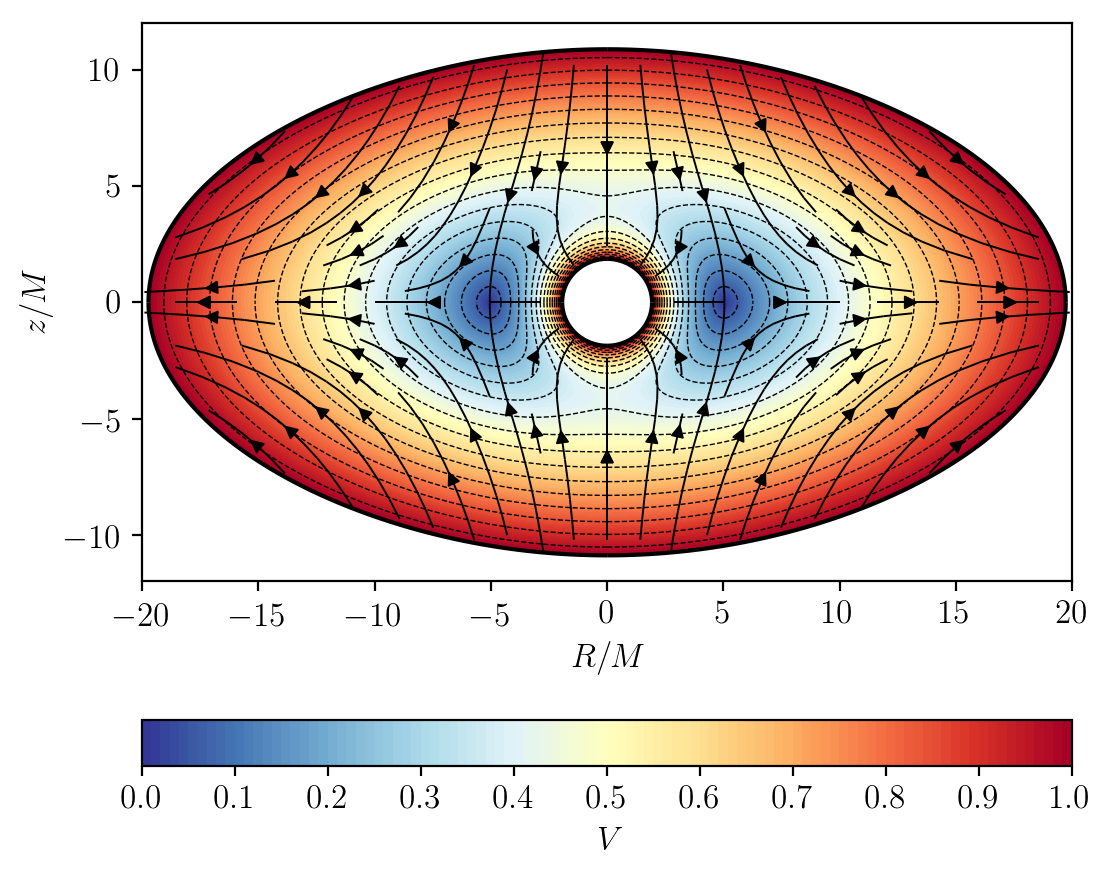
Figure 2: Same as in Fig. 1, except that $AM=-0.01$ is negative. The stagnation points in this case are located on an equatorial ring at a coordinate distance $r={\cal S}\simeq 5M$.

In both examples shown in Figs. 1 and  2, it is apparent that $V$ becomes luminal at two surfaces. From Eqs. (46a)-(46c), and as discussed in the previous section, it is simple to see that one such surface is the black hole’s event horizon located at $r=r_{+}$. This behavior is, however, a coordinate effect related to the fact that the ZAMOs become ill defined at this radius. Indeed, using Eqs. (21a)-(21d), it can be seen that the fluid’s four-velocity is completely regular across the event horizon.

On the other hand, the outer surface at which $V=1$ signals an unavoidable characteristic of the quadrupolar solution. This surface, that in what follows we shall refer to as $\cal E$, marks the transition of the gradient $\Phi_{,\mu}$ from being timelike (for points inner to $\cal E$) to becoming spacelike (for points outside $\cal E$). Moreover, from Eq. (50) we see that, at this surface, the density $\rho$ becomes zero and, for points outside $\cal E$, $\rho$ ceases to be a real quantity. For these reasons, we have to consider $\cal E$ as the outermost boundary delimiting the spatial domain of applicability of the quadrupolar solution.

An expression for $\cal E$ can be obtained by combining Eqs. (49) and (50), and rewrite the condition $V^{2}=1$ as the following second order polynomial in $\cos^{2}\theta$:

$$c_{2}(r)\,\cos^{4}\theta+c_{1}(r)\,\cos^{2}\theta+c_{0}(r)=0,$$ (54)

where

$$c_{0}(r) = r^{2}+2Mr+4M^{2}\left(\frac{r+r_{+}}{r-r_{-}}\right)$$ (55a)

$$-24AMr_{+}(r-M)-36A^{2}\Delta(r-M)^{2},$$

$$c_{1}(r) = a^{2}+72A(r-M)Mr_{+}$$ (55b)

$$-36A^{2}\big{[}\left(3\,r^{2}-6Mr+2M^{2}+a^{2}\right)^{2}$$

$$-6(r-M)^{2}\Delta\big{]},$$

$$c_{2}(r) = 36A^{2}\left(M^{2}-a^{2}\right)\left(3\,r^{2}-6Mr+4M^{2}-a^{2}\right).$$

From Eq. (54), one can show that, in the limit $AM\ll 1$ (which necessarily implies ${\cal S}\gg M$ and $r\gg M$), $\cal E$ reduces to the simple ellipsoid of revolution described by

$$r^{2}\left(1+3\,\cos^{2}\theta\right)=x^{2}+y^{2}+4\,z^{2}=\frac{1}{(6A)^{2}},$$ (56)

where, within this same limit, from Eq. (52) in Case 1 we have $A=M^{2}/(3\,{\cal S}^{3})$ while, from Eq. (53) in Case 2 it follows that $A=-2M^{2}/(3\,{\cal S}^{3})$.

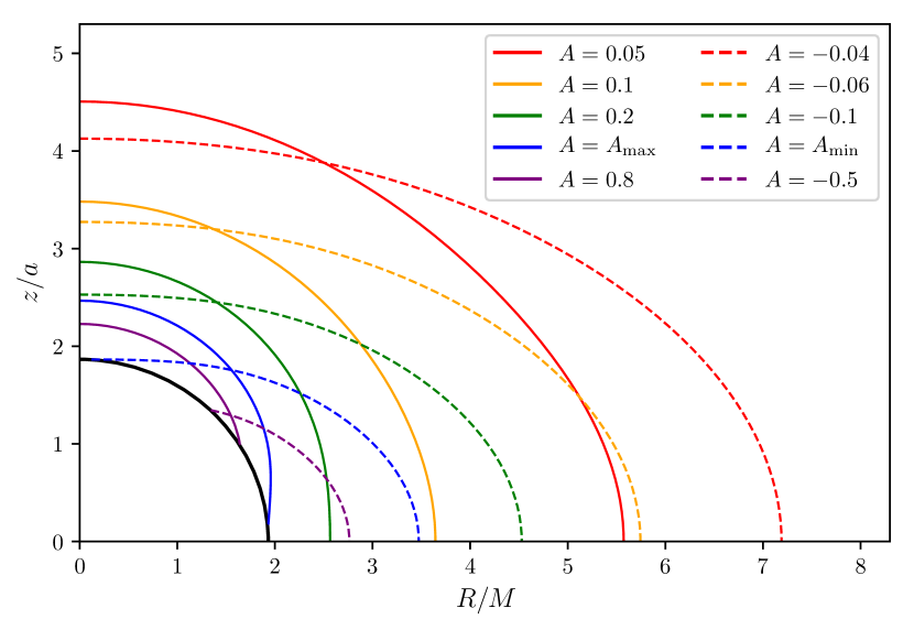
Figure 3: Outermost boundary $\cal E$ of the axisymmetric, quadrupolar flow for several values of the coefficient $A$. Solid, colored lines represent cases with $A>0$, while dashed colored lines correspond to $A<0$. The central black hole has a spin parameter $a=0.5M$. The event horizon is indicated by a solid black line. Note that the curves $\cal E$ corresponding to $A=A_{\max}\simeq 0.41$ and $A=A_{\min}\simeq-0.21$ touch the event horizon at the equator and pole, respectively. Curves with $A>A_{\max}$ or $A<A_{\min}$ actually pierce through the horizon. The axes correspond to the cylindrical-like coordinates $R=\sqrt{r^{2}+a^{2}}\,\sin\theta$, $z=r\,\cos\theta$.

On the other hand, by examining Eq. (54), it becomes apparent that, for a sufficiently large value of $|A|$, the surface $\cal E$ actually pierces through the event horizon. When $A>0$, $\cal E$ first touches the horizon at $\theta=\pi/2$ while, when $A<0$, $\cal E$ starts merging with the horizon at $\theta=0$. This means that the coefficient $|A|$ cannot be arbitrarily large or, in other words, that there is a minimum possible value ${\cal S}_{\min}$ for ${\cal S}$ such that ${\cal S}_{\min}>r_{+}$. In order to find the maximum value $A_{\max}$, let us first substitute $\theta=\pi/2$ in Eq. (54) and then evaluate the result at $r=r_{+}$. Doing this gives the condition $c_{0}(r_{+})=0$, which can be solved explicitly for $A$ as

$$A_{\max}=\frac{5M^{2}-a^{2}+3M\sqrt{M^{2}-a^{2}}}{24M(M^{2}-a^{2})}.$$ (57)

Similarly, for finding the minimum value $A_{\min}$, we substitute $\theta=0$ in Eq. (54) and then evaluate the result at $r=r_{+}$. This results in the condition $c_{2}(r_{+})+c_{1}(r_{+})+c_{0}(r_{+})=0$ which can be solved for $A$ as

$$A_{\min}=-\frac{M^{2}+M\sqrt{M^{2}-a^{2}}}{12M(M^{2}-a^{2})}.$$ (58)

For a Schwarzschild black hole, $A_{\max}=1/3$ (${\cal S}\simeq 2.32M$) and $A_{\min}=-1/6$ (${\cal S}\simeq 2.80M$). On the other hand, for a Kerr black hole with $a=0.5M$, we have $A_{\max}\simeq 0.41$ (${\cal S}\simeq 2.18M$) and $A_{\min}=-0.21$ (${\cal S}\simeq 2.61M$). Finally, note that in the extremal limit $a\rightarrow M$, $A$ actually becomes unbounded, i.e $(A_{\min},\,A_{\max})\rightarrow(-\infty,\,\infty)$. In Fig. 3 we show examples of the boundary $\cal E$ for different values of $A$ for a Kerr black hole with $a=0.5M$.

We conclude this section with some words regarding the case in which there is a misalignment between the accretion flow morphology and the black hole spin axis. As we show in further detail in the Appendix A, this case still allows for the same kind of inflow-outflow solutions. However, the resulting expressions become more involved as lack of axisymmetry forces us to consider, in addition to the $(\ell,m)=(2,0)$ mode, the contributions from the $m=-2,-1,1,2$ modes. As an example of the resulting accretion flow, in Fig. 4 we show the result of considering a misalignment angle of $\theta_{0}=30^{\circ}$ for the same flow parameters as in Fig. 1.

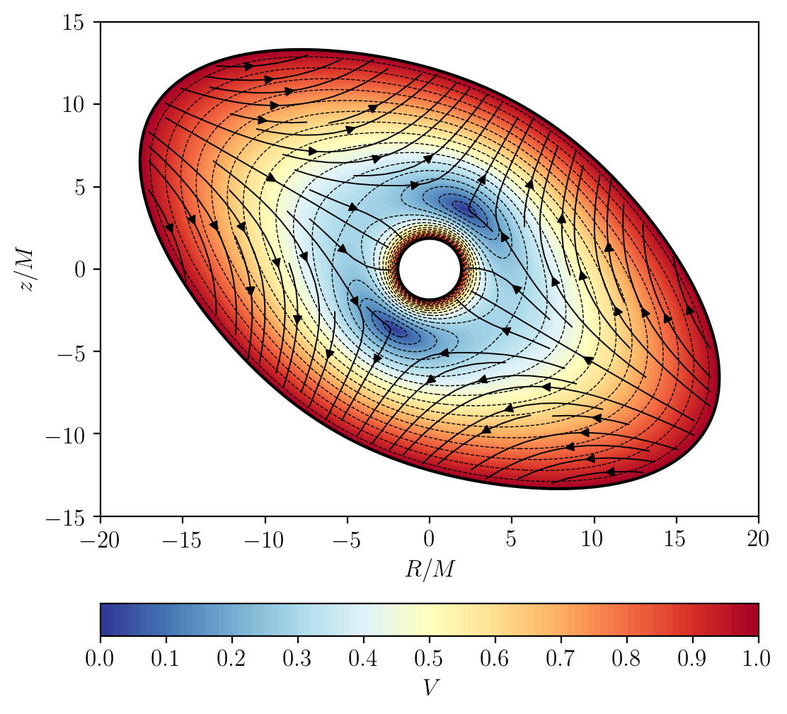
Figure 4: Same as in Fig. 1, except that now we consider an inclination angle $\theta_{0}=30^{\circ}$. In order to show the stagnation points, the plot corresponds to the plane $\phi=\phi(\epsilon)=-0.15882$ (see Table 2 and accompanying discussion).

IV Choked accretion

Here we apply the results obtained in the previous section to the choked accretion scenario discussed in TAH20 for a Schwarzschild spacetime. The idea is the following: a gas flow is injected radially inwards from points lying close to the equator of a sphere of certain coordinate radius $r={\cal R}>r_{+}$ (the “injection sphere”) toward the black hole. Part of this flow will be accreted by the black hole and disappears through the event horizon. However, when the injection rate is sufficiently large, it has been shown in TAH20 that (due to an anisotropic density field) part of the flow is diverted and ejected toward the poles. Under these conditions, the resulting flow is characterized by an inflow region originating from an equatorial belt in the injection sphere and a bipolar outflow region (Case 1 discussed in the previous section).

For the reasons mentioned in the introduction, we shall limit the rest of this work to the case in which the black hole’s angular momentum is perpendicular to the injection plane, that is, the equator of the injection sphere lies inside the equatorial plane $\theta=\pi/2$ of the Kerr spacetime.

For given values of the black hole parameters $(M,a)$, we characterize the resulting flow by specifying the fluid properties at the equator of the injection sphere, i.e., at $r=\mathcal{R},\ \theta=\pi/2$. At this reference point, we prescribe the thermodynamic variables $\rho_{0}=\rho(\mathcal{R},\pi/2)$, $h_{0}=h(\mathcal{R},\pi/2)$, and the magnitude of the fluid’s three-velocity $V_{0}$ as measured by a ZAMO at this location. See Fig. 5 for a schematic representation of the setup.

By imposing these boundary conditions in Eqs. (46a) and (48), it follows that

$$e = \Gamma_{0}h_{0}\mathcal{R}\sqrt{\frac{\Delta_{0}}{\Sigma_{0}}},$$ (59a)

$$A = \frac{\sqrt{\Sigma_{0}}\,V_{0}-2Mr_{+}}{6(\mathcal{R}-M)\Delta_{0}},$$ (59b)

where

$$\Delta_{0} = (\mathcal{R}-r_{-})(\mathcal{R}-r_{+}),$$ (60a)

$$\Sigma_{0} = (\mathcal{R}^{2}+a^{2})\mathcal{R}^{2}+2M\mathcal{R}a^{2},$$ (60b)

$$\Gamma_{0} = (1-V_{0}^{2})^{-1/2}.$$ (60c)

Figure 5: Schematic representation of the choked accretion model in the polar plane. Shown are the black hole region ($r<r_{+}$), the location of the injection sphere ($r=\mathcal{R})$, the location of the reference point $(r=\mathcal{R},\,\theta=\pi/2)$ where the data $(\rho_{0},h_{0},V_{0})$ characterizing the solution are specified, the location of the stagnation point at $r=\mathcal{S}$ and the critical angle $\theta_{c}$ which separates the inflow from the outflow regions on the injection sphere.

With the values for the model parameters in Eqs. (59a) and (59b), all of the results derived in the previous section can be directly adopted. In particular, the velocity field of the corresponding solution is given by Eqs. (46a)-(46c), the fluid enthalpy by Eq. (49), and the density field by Eq. (50). Also note that the location of the stagnation points in this case follows by combining Eq. (52) and Eq. (59b), which results in

$$\frac{\sqrt{\Sigma_{0}}\,V_{0}}{Mr_{+}}-2=\frac{({\cal R}-r_{-})({\cal R}-r_{+})({\cal R}-M)}{({\cal S}-r_{-})({\cal S}-r_{+})({\cal S}-M)}.$$ (61)

This equation can be explicitly solved for $\cal S$ as

$$\begin{split}\mathcal{S}=M+&\left(\xi+\sqrt{\xi^{2}-\frac{(M^{2}-a^{2})^{3}}{27}}\right)^{1/3}\\ +&\left(\xi-\sqrt{\xi^{2}-\frac{(M^{2}-a^{2})^{3}}{27}}\right)^{1/3},\end{split}$$ (62)

where

$$\xi=\frac{({\cal R}-r_{-})({\cal R}-r_{+})({\cal R}-M)Mr_{+}}{2(\sqrt{\Sigma_{0}}\,V_{0}-2Mr_{+})}.$$ (63)

Finally note that, following a procedure analogous to that described in TAH20 , one can obtain an expression for the projection of a streamline onto the $r$-$\theta$ plane given by

$$\Psi=\cos\theta\left[1+\frac{(r-r_{-})(r-r_{+})(r-M)}{(\mathcal{S}-r_{-})(\mathcal{S}-r_{+})(\mathcal{S}-M)}\frac{\sin^{2}\theta}{2}\right],$$ (64)

where $\Psi$ is an integration constant. Streamlines with $|\Psi|<1$ accrete onto the central black hole, those with $|\Psi|>1$ escape along the bipolar outflow, while those with $\Psi=1$ ($\Psi=-1$) are connected to the stagnation point at $\theta=0$ ($\theta=\pi$).

IV.1 Parameter range

The solution described by Eq. (44) with $e$ and $A$ as given in Eqs. (59a)-(59b) is characterized by six parameters: $M$ and $a$ describing the black hole, and $\cal R$, $\rho_{0}$, $h_{0}$ and $V_{0}$ specifying the boundary conditions at the injection sphere. As discussed in TAH20 , the obtained solution is actually scale-free with respect to the model parameters $M$ (that sets the overall length scale), $\rho_{0}$, and $h_{0}$ (that set the thermodynamic state of the fluid).

Once a Kerr background metric has been fixed with $M$ and $a$ (satisfying $|a|<M$), our next goal is to determine the range for the parameters $\cal R$ and $V_{0}$ leading to solutions that:

1. Are well-defined within the domain $r\in[r_{+},\ {\cal R}]$.

2. Present the inflow-outflow morphology of the choked accretion mechanism.

To this end, it is convenient to examine the ejection velocity defined as

$$V_{\rm ej}\equiv V^{\hat{r}}({\cal R},\,0)=\frac{2V_{0}\sqrt{\Sigma_{0}}-6Mr_{+}}{{\cal R}^{2}+a^{2}},$$ (65)

where we have used Eqs. (46a) and (59b).

Condition 1 is satisfied by requiring that the gradient of the potential function remains timelike within the domain of interest, which is equivalent to the condition that the right-hand side of Eq. (49) is positive for all $r\in[r_{+},{\cal R}]$ and all $\theta\in[0,\pi]$. In Appendix B we prove that this can be guaranteed by requiring

$${\cal R}\geq 3M+r_{+}$$ (66)

and demanding that $V_{\rm ej}<1$. From Eq. (65), this last condition in turn is equivalent to

$$V_{0}<\frac{{\cal R}^{2}+a^{2}+6Mr_{+}}{2\sqrt{\Sigma_{0}}}.$$ (67)

On the other hand, since we have already assumed inflow across the equator of the injection sphere, condition 2 is satisfied by requiring $V_{\rm ej}>0$. Again, from Eq. (65), this condition translates as

$$V_{0}>\frac{3Mr_{+}}{\sqrt{\Sigma_{0}}}.$$ (68)

Therefore, the injection velocity parameter is restricted as

$$V_{0}\in(V_{\min},\,V_{\max}),$$ (69)

with

$$V_{\min}=\frac{3Mr_{+}}{\sqrt{\Sigma_{0}}},\quad V_{\max}=\frac{{\cal R}^{2}+a^{2}}{2\sqrt{\Sigma_{0}}}+V_{\min}.$$ (70)

IV.2 Mass accretion, injection, and ejection rates

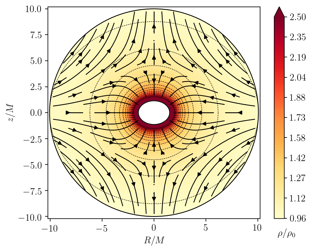
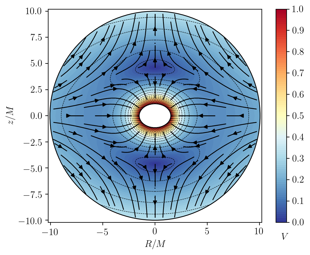
Figure 6: Analytic model of choked accretion for a Kerr black hole with $a=0.99\,M$ and flow parameters $\mathcal{R}=10\,M$ and $V_{0}=0.2$. The figure shows isocontours of the fluid’s normalized rest-mass density (left panel) as well as the magnitude of the three-velocity (right panel). The stagnation points are located on the symmetry axis with radius $\mathcal{S}\simeq 4.6011\,M$. Fluid streamlines are indicated by thick, solid lines with an arrow. The axes correspond to the cylindrical-like coordinates $R=\sqrt{r^{2}+a^{2}}\,\sin\theta$ and $z=r\,\cos\theta$.

The accretion rate follows by substituting Eq. (59a) into Eq. (41), which results in

$$\dot{M}=8\pi Mr_{+}\frac{\rho\,e}{h}=8\pi Mr_{+}\Gamma_{0}\,\rho_{0}\,\mathcal{R}\sqrt{\frac{\Delta_{0}}{\Sigma_{0}}}.$$ (71)

By considering the flux of mass across the injection sphere, we can distinguish between the inflow and outflow fluxes, $\dot{M}_{\rm in}$ and $\dot{M}_{\rm ej}$, respectively, defined in such a way that

$$\dot{M}_{\rm in}-\dot{M}_{\rm ej}=\dot{M}.$$ (72)

We can calculate both fluxes explicitly by examining the radial component of the fluid velocity at the injection sphere. From Eq. (46a), it follows the existence of a critical angle $\theta_{c}$ given by

$$\theta_{c}=\arccos\left[3\left(1-\frac{2Mr_{+}}{\sqrt{\Sigma_{0}}V_{0}}\right)\right]^{-1/2},$$ (73)

such that there is inflow ($V^{\hat{r}}<0$) for the equatorial belt defined by $\theta\in(\theta_{c},\,\pi-\theta_{c})$ and outflow ($V^{\hat{r}}>0$) for the polar regions $\theta\in(0,\,\theta_{c})$ and $\theta\in(\pi-\theta_{c},\,\pi)$.

We can thus calculate $\dot{M}_{\rm in}$ in terms of $\theta_{c}$ as

$$\dot{M}_{\rm in}=-4\pi\int_{\theta_{c}}^{\pi/2}\rho\,U^{r}\varrho^{2}\sin\theta\,\mathrm{d}\theta=\Lambda\dot{M}$$ (74)

where

$$\Lambda=\frac{2\cos^{3}\theta_{c}}{3\cos^{2}\theta_{c}-1}=\frac{\sqrt{\Sigma_{0}}V_{0}}{3\sqrt{3}Mr_{+}}\left(1-\frac{2Mr_{+}}{\sqrt{\Sigma_{0}}V_{0}}\right)^{-1/2}.$$ (75)

Clearly, in view of Eq. (72), it follows that

$$\dot{M}_{\rm ej}=(\Lambda-1)\dot{M}.$$ (76)

In Fig. 6 we show the isocontour levels of the rest-mass density field, as well as the magnitude of the three-velocity $V$, and the resulting fluid streamlines (black solid arrows) for a representative case with model parameters $a=0.99\,M$, $\mathcal{R}=10\,M$, and $V_{0}=0.2$.

In Fig. 7 we represent the regions in the parameter space $(a,\,V_{0})$ that lead to the choked accretion solution as discussed in Sec. IV.1. The plotted isocontours correspond to the mass accretion rate $\dot{M}$ expressed in units of $\dot{M}_{0}=8\pi M^{2}\rho_{0}$. Each panel corresponds to a different value of the injection radius ${\cal R}$, from top to bottom ${\cal R}/M=4,\,8,\,100$. The boundary lines delimiting each region correspond to the $V_{\min}$ and $V_{\max}$ limits given in Eq. (70). From this figure we can see a general trend for increasing values of $\dot{M}$ as the value of $V_{0}$ increases, while $\dot{M}$ decreases as the spin parameter $a/M$ grows from zero to 1. Also note that the dependence on $a$ of the limits $V_{\min}$ and $V_{\max}$ becomes less noticeable as increasingly larger values of ${\cal R}$ are considered.

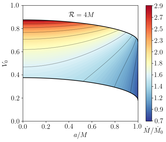
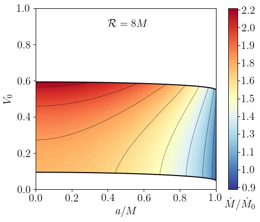
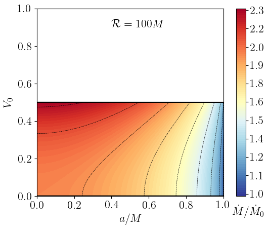
Figure 7: Mass accretion rate as a function of the model parameters ($a$, $V_{0}$) in units of $\dot{M}_{0}=8\pi M^{2}\rho_{0}$. The value of the injection radius ${\cal R}$ in each case is indicated by a central label on each panel. The solid, black lines in each panel indicate the range of validity of the model parameters according to $V_{0}\in(V_{\min},\,V_{\max})$, with the lower boundary corresponding to $V_{\min}$ and the upper one to $V_{\max}$.

In Fig. 8 we show three different properties of the choked accretion model as a function of the spin parameter $a/M$, for an injection sphere at $\mathcal{R}=10\,M$. Each color line represents a different value of the injection velocity. The quantities correspond to: the mass accretion rate $\dot{M}$ (in units of $\dot{M}_{0}$) in the top panel, the location of the stagnation points $\mathcal{S}$ in the middle panel, and the ejection-to-injection mass rate ratio $\eta=\dot{M}_{\rm{ej}}/\dot{M}_{\rm{in}}$ in the bottom panel. For comparison, in the top panel we also show, in a black solid line, the accretion rate for the “spherically symmetric” case $(\ell,m)=(0,0)$ corresponding to $A=0$ and $V_{0}=2Mr_{+}/\sqrt{\Sigma_{0}}$ (note that there is no ejection for $V_{0}$ in the range between this value and $V_{\min}$).

From the previous discussion we note that, as the injection velocity grows from $V_{\min}$ to $V_{\max}$, we have:

• The radii of the stagnation points decrease from ${\cal S}={\cal R}$ to ${\cal S}_{\min}$.

• The critical angle increases from $\theta_{c}=0$ to

  $$\theta_{\max}=\arccos\left[3\left(\frac{{\cal R}^{2}+a^{2}+2Mr_{+}}{{\cal R}^{2}+a^{2}+6Mr_{+}}\right)\right]^{-1/2},$$ (77)

  that, in the limit ${\cal R}\gg M$, converges to $\theta_{\max}=\arccos(1/\sqrt{3})\simeq 54.7^{\circ}$.

• The mass injection rate increases from $\dot{M}_{\rm in}=\dot{M}$ to

  $$\dot{M}_{\rm in}=\frac{\left[\frac{1}{3}\left(1+\frac{4Mr_{+}}{({\cal R}-r_{+})({\cal R}-r_{-})}\right)\right]^{3/2}}{\frac{2Mr_{+}}{({\cal R}-r_{+})({\cal R}-r_{-})}}\dot{M}.$$ (78)

On the other hand, from Figs. 7 and 8, we note that, as the spin parameter $a/M$ increases from zero to 1, the mass accretion rate onto the central black hole decreases down to $\sim 50\%$, the location of the stagnation point $S$ decreases by a factor of $\sim 10\%$, while the ejection-to-injection mass rate ratio $\eta$ increases by up to $\sim 30\%$.

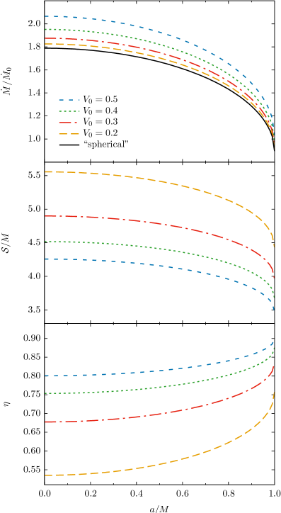
Figure 8: Dependence of different properties of the choked accretion model on the spin parameter $a/M$ and the injection velocity $V_{0}$, for an injection sphere at $\mathcal{R}=10\,M$. From top to bottom, each panel shows: the mass accretion rate $\dot{M}$ in units of $\dot{M}_{0}=8\pi M^{2}\rho_{0}$, the location of the stagnation points $\mathcal{S}/M$, and the ejection-to-injection mass rate ratio $\eta=\dot{M}_{\mathrm{ej}}/\dot{M}_{\mathrm{in}}$. The black line in the first panel corresponds to the “spherical” case $(\ell,m)=(0,0)$, for which $V_{0}=2Mr_{+}/\sqrt{\Sigma_{0}}\,\simeq 0.0003.$

The analytic model studied in the previous sections allows us to explore in detail the effect of the black holes’s rotation on the choked accretion mechanism. Unfortunately, this model cannot easily be extended to perform a more general study including a more realistic equation of state. Keeping the irrotational assumption one can still formulate the problem in terms of a scalar potential; however, this potential satisfies a wave equation which is nonlinear for a realistic equation of state. Clearly, this makes it much harder to find an analytic treatment. For this reason, in the next section, we extend our study to the case of a general polytropic fluid by performing numerical simulations of the choked accretion scenario.

V Numerical simulations

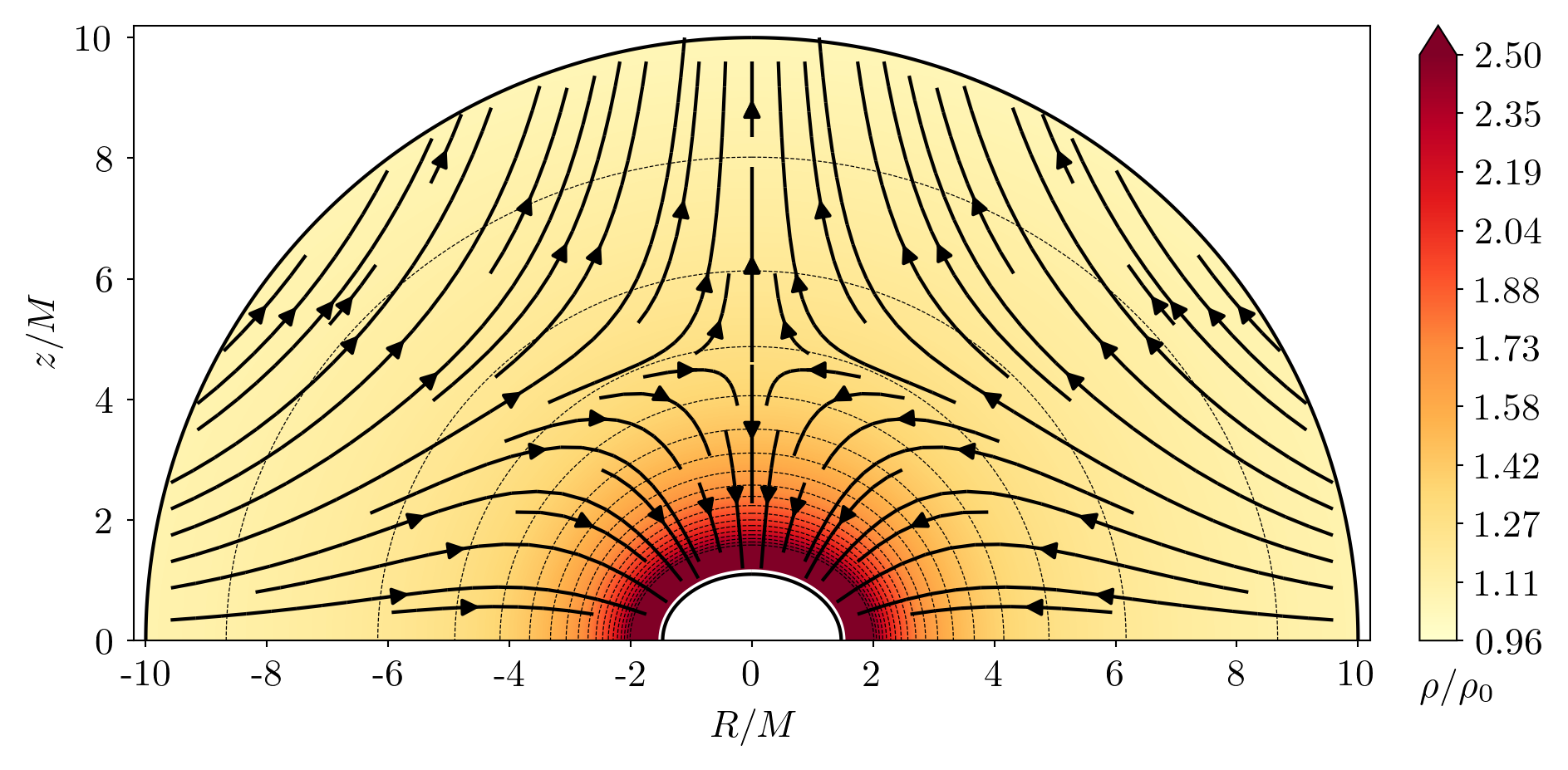
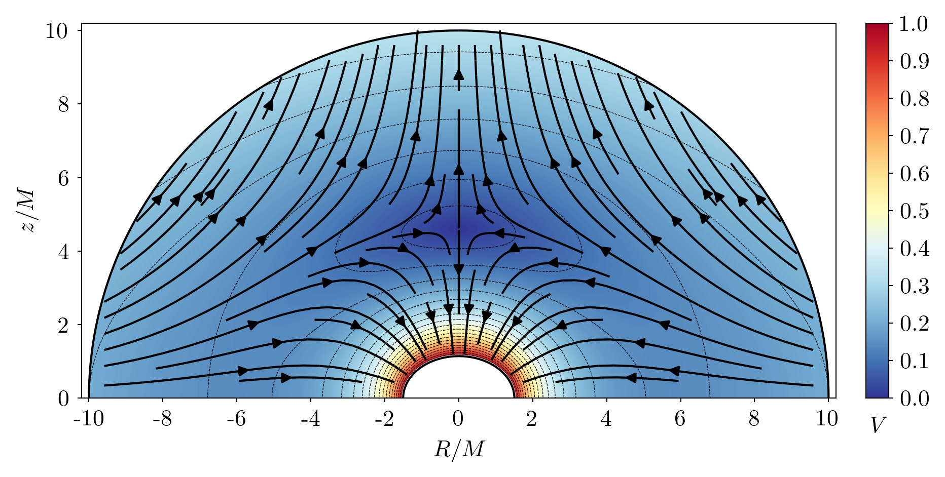
Figure 9: Validation test of the aztekas code. In this figure we show the steady state of numerical simulation for the benchmark test, which corresponds to the analytic solution presented in Sec. IV, with parameters $\mathcal{R}=10\,M$, $V_{0}=0.2$, and $a=0.99M$ (compare with Fig 6). The figure shows the isocontour levels of the normalized rest-mass density $\rho/\rho_{0}$ (left panel) and the magnitude of the three-velocity (right panel) $V$, as measured by a ZAMO at this location. The fluid streamlines are indicated with black solid arrows. The simulation reached the stationary state at $t=180\,M$, showing a good agreement with the analytic solution.

The general solution presented by Petrich, Shapiro and Teukolsky lPsSsT88 revisited in Sec. II and, in particular, the choked accretion scenario discussed in Sec. IV, are limited by the assumption of an ultrarelativistic gas with a stiff equation of state, which leads to an unphysical speed of sound. In this section we show, by means of full hydrodynamic numerical simulations, that the main features of the choked accretion model are maintained when the adopted equation of state is extended to consider a general polytropic gas. Moreover, we make use of the analytical solution presented above as a 2D benchmark test for the validation of the code.

We perform full hydrodynamic numerical simulations with the open source code aztekas (aguayo18, ; eTaA19, ), which solves the general relativistic hydrodynamic equations using a grid based finite volume scheme, with a High Resolution Shock Capturing (HRSC) method. The set of equations are written in a conservative form using a variation of the “3+1 Valencia formulation” fBjaFjmIjmMjaM97 for time independent, fixed metrics lDZoZnBpL07 . The time integration is achieved by adopting a second order total variation diminishing Runge-Kutta method cwSsO88 . The fluid evolution is performed in a fixed background metric corresponding to a Kerr black hole using the same (horizon-penetrating) Kerr-type coordinates adopted in Sec. II. The code uses as primitive variables the rest-mass density, pressure and the locally measured three-velocity vector $(\rho,P,v_{i})$, where $v_{i}=\gamma_{ij}v^{j}$ and

$$v^{i}=\frac{U^{i}}{\alpha U^{t}}+\frac{\beta^{i}}{\alpha},\qquad i=r,\theta,\phi,$$ (79)

with $\alpha$, $\beta^{i}$ and $\gamma_{ij}$ the lapse, shift vector and three-metric of the 3+1 formalism mA08 , written in these coordinates. See aguayo18 ; eTaA19 ; aAeTxH19 ; TAH20 , for more details about the characteristics, test suite, and discretization method of aztekas.

For all the simulations presented in this section, we adopt an axisymmetric 2D numerical domain $(r,\theta)\in[\mathcal{R}_{\mathrm{acc}},\mathcal{R}]\times[0,\pi/2]$, with a uniform polar grid and an exponential radial grid (see aAeTxH19 for details), where $\mathcal{R}$ is the radius of the outer boundary at which we implement a free outflow condition for the velocities and a fixed profile for the density and pressure. The inner boundary, set at $\mathcal{R}_{\text{acc}}=1.1\,M$, for which we impose free outflow in all the variables, is chosen such that $r_{-}<\mathcal{R}_{\mathrm{acc}}<r_{+}$ for all the explored values of $a$. We fix reflection conditions at both polar boundaries. A dissipative, second-order piecewise linear reconstruction for the primitive variables is used in order to avoid spurious oscillations due to these fixed boundary conditions.

In all the simulations, we evolve the equations from an initial state consisting of a constant density and pressure gas cloud, with zero initial three-velocity $v_{i}=0$. The convergence to a steady-state is monitored by computing the mean mass accretion rate $\dot{M}$ all over the domain, until its variation drops below 1 part in $10^{4}$.

V.1 Benchmark test

Taking advantage of the exact analytic description presented in the previous sections, we use the solution in Eq. (44) as a benchmark test to prove the convergence and stability of the aztekas code for this type of problems. Moreover, this test is important in order to validate the subsequent simulations discussed in this article. For these tests we implement the ultrarelativistic stiff equation of state in the numerical code.

We reproduce the analytic solution corresponding to the choked accretion model with $\mathcal{R}=10M$, $V_{0}=0.2$ and a black hole spin $a=0.99M$. We run the simulations in units such that $M=1$ and set the value $\rho_{0}=1$ for the density at the reference point, although we remark here that, just as in the analytic case, the resulting steady-state solution is scale-free with respect to this specific value of $\rho_{0}$. We perform four tests varying the spatial resolution by a factor of 2 each time (with number of grid points in the radial and polar directions $64\times 64$, $128\times 128$, $256\times 256$, $512\times 512$, respectively). The values for $(\rho,P,v_{i})$ from the analytic solution are imposed at the injection sphere as the boundary condition, and these values are extended into the whole numerical domain as the initial condition.

In Fig. 9 we show the isocontour levels of the density field and of the magnitude of the three-velocity $V$ (as measured by a ZAMO) of the aztekas simulations when the steady-state is reached at $t=180\,M$. Likewise, the streamlines of the stationary flow are shown in both figures. From these simulations we obtain the stagnation point at $\mathcal{S}\simeq 4.6015\,M$ which coincides with the analytical value within the resolution uncertainty (see Fig. 6).

In Fig. 10 we show the evolution in time of the relative error between the numerical mass accretion rate $\dot{M}$ and the analytic value $\dot{M}_{\mathrm{A}}$, for all of the resolutions considered here. As expected, the relative error decreases for larger resolutions. Indeed, as further shown in Appendix C, from this benchmark test we confirm a second order convergence rate, as expected from the adopted numerical scheme.

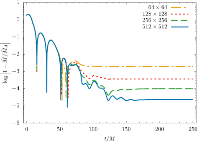
Figure 10: Validation test for the aztekas code. In this figure we show the evolution in time of the relative error between the numerical mass accretion rate $\dot{M}$ and analytic value $\dot{M}_{A}$ for the solution with parameters $\mathcal{R}=10\,M$, $V_{0}=0.2$, and $a=0.99M$. The four different resolutions used for this benchmark test are represented with different dashed lines, showing a diminishing of the error as the resolution increases which, as shown in Appendix C, is consistent with second order convergence.

V.2 Polytropic fluid

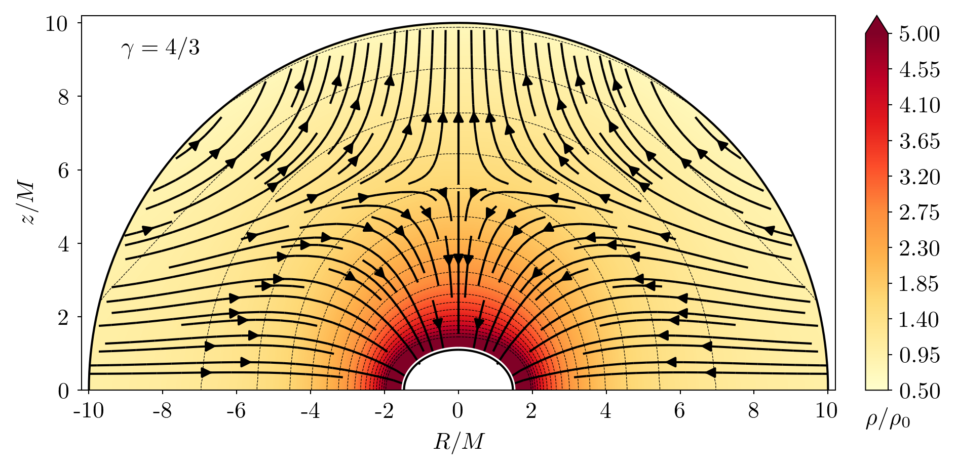
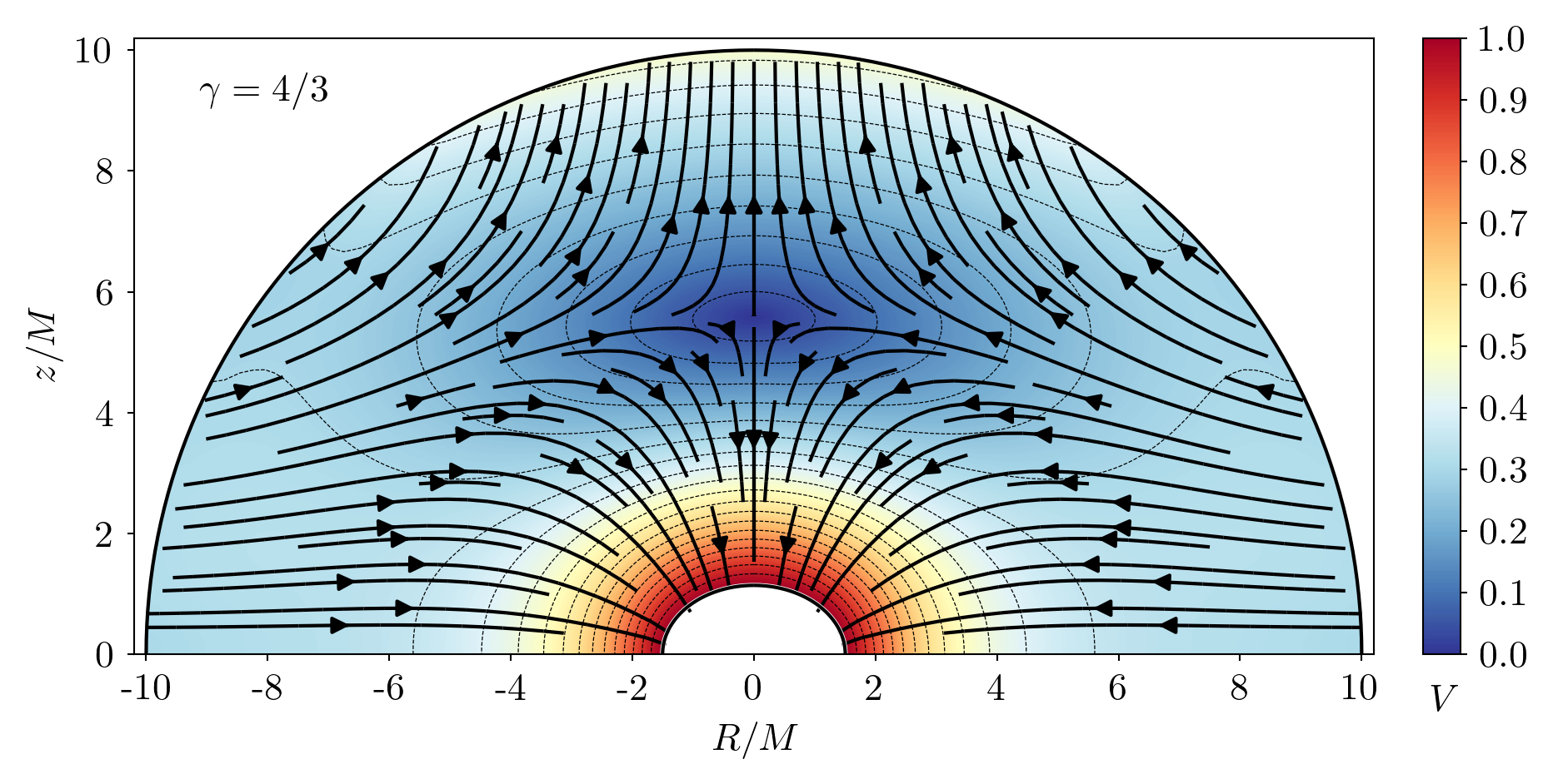
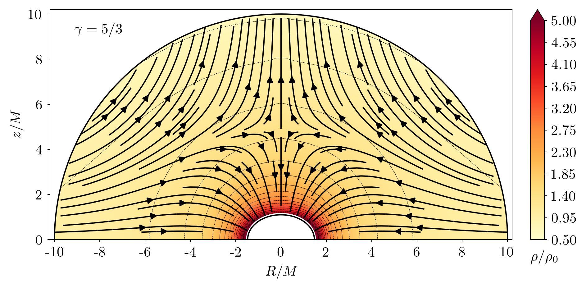
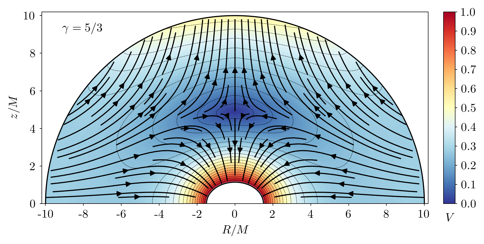
Figure 11: Stationary state of the numerical simulations of the choked accretion mechanism for a rotating black hole with $a=0.99M$, an injection radius of $\mathcal{R}=10M$, a dimensionless temperature of $\Theta_{0}=1$ at the equator of the injection sphere, and a polytropic fluid with $\gamma=4/3$ (top panels) and $5/3$ (bottom panels). On the left panels of this figure we show the isocontour levels of the normalized rest-mass density $\rho/\rho_{0}$ while, on the right panels, the magnitude of the three-velocity $V$ as measured by the ZAMO. The fluid streamlines are indicated with black solid arrows, while a white solid line shows the location of the event horizon $r_{+}$.

In order to explore the behavior of the choked accretion mechanism for a gas with a less restrictive equation of state, we perform numerical simulations of an ideal gas with a polytropic relation $P=K\rho^{\gamma}$, where $\gamma$ is the adiabatic index. We run experiments using a $256\times 256$ grid resolution, for a wide range of values of the spin parameter $a/M\in[0,1)$ and two different values of the adiabatic index $\gamma\in\left\{4/3,5/3\right\}$.

The main feature of the choked accretion mechanism relies on the existence of a density contrast at the external boundary. Following closely the boundary treatment of aAeTxH19 ; TAH20 , we fix the gas rest-mass density at the outer boundary as

$$\rho_{\mathrm{b}}(\theta)=\rho_{0}(1-\delta\cos^{2}\theta),$$ (80)

where $\rho_{0}$ is the rest-mass density at the reference point $(\mathcal{R},\pi/2)$ and $\delta$ is the density contrast defined as

$$\delta=1-\frac{\rho_{b}(0)}{\rho_{0}}.$$ (81)

As mentioned in Sec. I, this density profile is motivated as a way to introduce the axisymmetric anisotropy associated with fluid rotation. In particular, it has been shown that low angular momentum fluids accreting onto a central massive object give rise to a quasi-spherical, oblate density distribution, as long as the angular momentum is sufficiently low as to avoid encountering the centrifugal barrier (proga2003, ; mach2018, ).

The pressure at this boundary is then determined by the polytropic relation $P=K\rho^{\gamma}$, where $K$ is computed as eTaA19

$$K=\frac{1}{\rho_{0}^{\gamma-1}}\left[\frac{c_{0}^{2}(\gamma-1)}{\gamma(\gamma-1)-c_{0}^{2}}\right]$$ (82)

with $c_{0}$ the speed of sound at the reference point.

An extensive exploration of the choked accretion mechanism’s dependence on $\mathcal{R}$, $\delta$ and $c_{0}$ can be found in aAeTxH19 for the non-relativistic regime and in TAH20 for the case of a Schwarzschild black hole. We performed a quick exploration of these three parameters, for a rotating black hole with $a=0.99M$, and found essentially the same results as reported in those previous works. Moreover, we noticed that it is more intuitive, in order to compare with possible astrophysical settings, to use the dimensionless temperature $\Theta_{0}=P_{0}/\rho_{0}$ rather than specifying $c_{0}$. For this reason, in what follows, we shall take as representative values $\mathcal{R}=10M$ for the domain size, $\delta=0.5$ for the density contrast and $\Theta_{0}=1$ for the temperature of the gas at the reference point. This value of the dimensionless temperature corresponds to $c_{0}\approx 0.52$ and $c_{0}\approx 0.69$, for $\gamma=4/3$ and $5/3$, respectively. Furthermore, in order to have an appropriate baseline reference for each combination of the $\gamma$ and $a$ parameters, we also run simulations corresponding to “spherical” accretion in each case (i.e., same values for $\gamma$ and $a$ but a $\delta=0$ density contrast).

We evolve all the simulations until the stationary state has been reached (within the previously mentioned limit of accuracy in which variations in the mean accretion rate drop below $1$ part in $10^{4}$). The relaxation time depends on $\gamma$, as well as on the value of $a$, but in all cases it is found to conform to $500\,M<t<1500\,M$. We also perform a self-convergence test which is presented in Appendix C.

In Fig. 11 we show the resulting steady-state, rest-mass density field and magnitude of the three-velocity $V$ for the $a=0.99\,M$ case. The top panels show the results corresponding to $\gamma=4/3$ while the bottom panels those for $\gamma=5/3$. The black solid arrows represent the fluid streamlines and the solid white line the location of the outer horizon $r_{+}$. As we can see from these figures, there is not a strong qualitative difference in the flow morphology for different values of $\gamma$, neither for the one presented in the non-rotating black hole case TAH20 . Moreover, although the streamlines configuration are similar to the analytical case, the ejection velocity at the polar region is larger for the polytropic fluid (see Fig. 6).

In Fig. 12 we show the dependence of the mean mass accretion rate $\dot{M}$ on the spin parameter $a$, for all the simulations performed in this study. The blue dots correspond to $\gamma=4/3$, while the red crosses to $\gamma=5/3$. The points joined by the dashed lines represent the corresponding “spherical” accretion case ($\delta=0$). It is interesting to notice from this figure that, for each value of $\gamma$, the dependence on $a$ remains the same regardless of the value of $\delta$ (except for a re-scaling factor that depends on $\gamma$). This suggest that the change in the mass accretion rate with the spin parameter is an intrinsic characteristic of the accretion onto a Kerr black hole, and not of the choked accretion mechanism. A more complete study of the “spherical” accretion case onto a rotating black hole will be explored elsewhere.

In addition to the mass accretion rate, we compute the mass injection rate $\dot{M}_{\mathrm{in}}$ and the mass ejection rate $\dot{M}_{\mathrm{ej}}$ at the injection sphere (as defined in Sec. IV.2). We also extract from the simulation’s results the location of the stagnation point $\mathcal{S}$. In Table 1 we present a summary of these results for a representative set of the performed simulations. We also measure the magnitude of the three-velocity at the equator $V_{0}$ and at the pole $V_{\mathrm{ej}}$, which do not present a significative dependence on the spin parameter, maintaining a value around $V_{0}=0.30$ and $V_{\mathrm{ej}}=0.54$, for $\gamma=4/3$; and $V_{0}=0.29$ and $V_{\mathrm{ej}}=0.48$, for $\gamma=5/3$.

In Fig. 13 we show the dependence on $a$ for the mass accretion rate $\dot{M}$ (top panel), the location of the stagnation point $\mathcal{S}$ (middle panel), and the ejection-to-injection mass rate $\eta$ (bottom panel), for both values of $\gamma$. In order to clearly see the change with $a$ for these quantities, we normalize them by $\dot{M}_{\mathrm{S}}$, $\mathcal{S}_{\mathrm{S}}$ and $\eta_{\mathrm{S}}$, respectively, which correspond to the values obtained in the non-rotating case ($a=0$). Moreover, we also include the stiff analytic solution obtained in Sec. IV, using as the $V_{0}$ parameter the value found for $\gamma=5/3$.

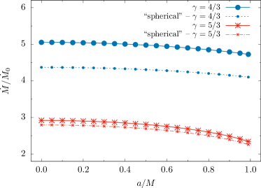
Figure 12: Mass accretion rate as a function of the spin parameter. The blue and red dotted lines correspond to $\gamma=4/3$ and $5/3$, respectively. The black dashed lines represent their respective “spherical” accretion values, i.e., $\delta=0$.

Table 1: Results for our simulations with parameters $\mathcal{R}=10\,M$, $\delta=0.5$ and $\Theta_{0}=1$.

	$\gamma=4/3$				$\gamma=5/3$
$a/M$	$\mathcal{S}/M$	$\dot{M}$	$\dot{M}_{\mathrm{ej}}$	$\dot{M}_{\mathrm{in}}$	$\mathcal{S}/M$	$\dot{M}$	$\dot{M}_{\mathrm{ej}}$	$\dot{M}_{\mathrm{in}}$
0.0	5.781	5.052	2.195	7.246	5.247	2.919	2.768	5.687
0.25	5.770	5.033	2.201	7.234	5.231	2.892	2.777	5.670
0.5	5.734	4.977	2.220	7.197	5.179	2.808	2.805	5.614
0.75	5.672	4.876	2.256	7.132	5.083	2.647	2.857	5.504
0.99	5.581	4.725	2.308	7.032	4.905	2.343	2.947	5.289

NOTE – The quantities $\dot{M}$, $\dot{M}_{\mathrm{in}}$ and $\dot{M}_{\mathrm{ej}}$ are given in units of $\dot{M}_{0}=8\pi M^{2}\rho_{0}$.

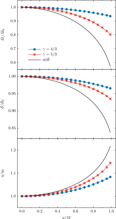
Figure 13: Dependence of different properties of the choked accretion simulations on the spin parameter $a/M$ and $\gamma$. From top to bottom, each panel shows: the mass accretion rate $\dot{M}$, the location of the stagnation point $\mathcal{S}/M$, and the ejection-to-injection mass rate ratio $\eta=\dot{M}_{\mathrm{ej}}/\dot{M}_{\mathrm{in}}$. Each panel is normalized by its corresponding non-rotating case value, which is denoted with the subscript $\mathrm{S}$. The black solid line represents the analytic solution presented in Sec. IV for a ultrarelativistic stiff fluid.

As we can see from Fig. 13, the mass accretion rate decreases with the spin parameter down to a factor of $\sim 10\%$ (20%) for the $\gamma=4/3$ ($\gamma=5/3$) case as the spin parameter increases to its maximum value. On the other hand, the location of the stagnation point only decreases down to a factor of $\sim 5$% for both values of $\gamma$. In contrast, the ejection-to-injection mass rate $(\eta)$ increases up to a factor of 10 to 15% as $a\to M$.

Even though it is not possible to make a direct comparison of the numerical simulations with the analytic model of an ultrarelativistic stiff fluid, since in each case we are using different equations of state and the boundary conditions are not exactly the same, there are still some observations that can be drawn from Fig. 13. First of all, there is a shared, qualitatively consistent dependence of the different quantities shown in this figure on the spin parameter $a$, both for the polytropic gas and the stiff fluid. Moreover, it is also clear that there is a stronger response from the stiff fluid to the black hole rotation. Indeed, from this figure we see that the analytic solution presented in Sec. IV can be used as a lower limit for the mass accretion rate and for the location of the stagnation point that would follow for a polytropic gas, whereas it can be used as an upper limit for the ejection-to-injection mass rate ratio. Finally, we note that there is a clear trend for a stronger dependence on the spin parameter $a$ as the fluid stiffens ($\gamma\to 2$).

VI Summary and conclusions

The choked accretion model is a purely hydrodynamical mechanism with which it is possible to obtain a bipolar outflow by perturbing an originally radial inflow. The necessary conditions for this mechanism to operate consist of a sufficiently large mass accretion rate onto a central massive object (as compared to the Bondi accretion rate), and an anisotropic density field in which the equatorial region is at a higher density than at the poles. Potential astrophysical applications of this model for outflow-generating phenomena are mentioned in the introduction and have been discussed in further detail in aAeTxH19 ; TAH20 .

In this article we have presented a generalization of the choked accretion mechanism for the case of a rotating Kerr black hole, extending the perturbative study initiated by Hernandez et al. hernandez14 and the subsequent analytical and numerical studies at the non-relativistic level aAeTxH19 and in the Schwarzschild case TAH20 . Here we have shown, using both analytic solutions and numerical simulations, that the choked accretion’s main features are recovered in the presence of a rotating black hole, regardless of the value of the spin parameter.

Our analytic model is based on the steady-state, irrotational solution for an ultrarelativistic stiff fluid presented by Petrich, Shapiro and Teukolsky lPsSsT88 . We have derived the general equations of the model using horizon-penetrating Kerr-type coordinates and then mostly focused on the axisymmetric quadrupolar case, studying the dependence of the flow morphology on the unique parameter $A$ that remains free (we have also briefly discussed the misaligned quadrupolar case at the end of Sec. III and in Appendix A). Depending on the sign of this parameter, the flow describes an equatorial inflow-bipolar outflow solution ($A>0$) or an equatorial outflow-polar inflow solution ($A<0$). Given that it has a wider applicability in an astrophysical context and corresponds to the choked accretion scenario discussed in this article, we have mainly focused on the case $A>0$ and discussed the physical properties of the choked accretion model, including its mass accretion rate, location of the stagnation points and ejection-to-injection mass rate ratio. We have also extended the present study to a perfect fluid obeying a polytropic relation with adiabatic index $\gamma=4/3$ and $5/3$, by performing full hydrodynamic, relativistic numerical simulations of an ideal gas in a Kerr background metric.

In previous works, it was found that the total mass accretion rate in the choked accretion model has a threshold value close to the one found in the spherical accretion scenario. In this study, based on both analytic and numerical analysis, we have extended this result to the case of a rotating black hole and shown that the accretion rate obtained from the “spherically symmetric” case, in which the density contrast is set to zero at the injection sphere, still yields a lower limit for the threshold value for the choking mechanism to work (see Figs. 8 and 12). Note, however, that in the case of the Kerr spacetime there is no analytic equivalent to Michel’s solution in the Schwarzschild case. Therefore, this problem has to be studied by numerical means as we have briefly discussed here and will further address in a future work.

Most of the configurations analyzed in this article have focused on the aligned case, in which the axis of the bipolar outflow coincides with the rotation axis of the black hole, in which case the fluid elements have zero angular momentum and hence would not affect the black hole’s spin during their accretion. However, in Appendix A we have also analyzed a misaligned configuration, and it is interesting to note that such an accretion flow would slow down the black hole’s rotation, as the results in Sec. II.3 show.

This work continues a series of analytic and numerical studies of the choked accretion model as a purely hydrodynamical mechanism for generating axisymmetric outflows. In future work we intend to expand the ingredients involved in this model, by including additional physics such as fluid angular momentum, viscous transport, and magnetic fields, in order to explore the applicability of the model in outflow-generating astrophysical systems.

Appendix A The misaligned quadrupolar flow

In Sec. III we discussed the axisymmetric quadrupolar flow solution and some important properties regarding its morphology, and in Sec. IV this solution was applied to the choked accretion scenario. This flow has the property of being reflection-symmetric about the equatorial plane of the Kerr black hole, such that the bipolar outflow regions are aligned with the symmetry axis. In this appendix, we discuss an example in which the flow discussed in Secs. III and IV is “rotated” by an angle $\theta_{0}$ about an axis within the plane $\theta=\pi/2$ (in a sense made precise below).

When the black hole is non-rotating, the aforementioned rotation can be carried out exactly and is simply a rigid rotation of the (spherically symmetric) Schwarzschild geometry the Kerr metric reduces to in the limit $a=0$. We may construct this rotated solution explicitly by writing the angular dependency in the axisymmetric quadrupolar flow solution (45) in the form

$$3\cos^{2}\theta-1=2P_{2}(\cos\theta)=2P_{2}({\bf x}^{\prime}\cdot{\bf x}),$$ (83)

with $P_{2}$ denoting the Legendre polynomial $P_{\ell}$ with $\ell=2$ and ${\bf x}=(\sin\theta\cos\phi,\sin\theta\sin\phi,\cos\theta)$ and ${\bf x^{\prime}}:=(0,0,1)$. Applying a rotation by the angle $\theta_{0}$ about the $y$ axis is equivalent to replacing the vector ${\bf x}^{\prime}=(0,0,1)$ with the vector ${\bf x}^{\prime}=(\sin\theta_{0},0,\cos\theta_{0})$ in the right-hand side of Eq. (83). Recalling the addition theorem for spherical harmonics (see, for instance, chapter 3.6 in Ref. Jackson-Book )

$$P_{\ell}({\bf x}^{\prime}\cdot{\bf x})=\frac{4\pi}{2\ell+1}\sum\limits_{m=-\ell}^{\ell}(Y^{\ell m})^{*}(\theta^{\prime},\phi^{\prime})Y^{\ell m}(\theta,\phi),$$ (84)

we can write the rotated quadrupolar flow solution on a Schwarzschild background as in Eq. (44) with $a=0$ and $F(r,\theta,\phi)$ given by

$$F(r,\theta,\phi)=\frac{8\pi}{5}(3r^{2}-6Mr+2M^{2})\sum\limits_{m=-\ell}^{\ell}d_{m}Y^{\ell m}(\theta,\phi)$$ (85)

with the coefficients $d_{m}:=(Y^{\ell m})^{*}(\theta_{0},0)$. This has again the form of the general solution in Eq. (17) when $a=0$, and hence it describes a solution of the potential flow equation (1). However, it bears exactly the same physical content as the original axisymmetric quadrupolar flow solution discussed in Secs. III and IV, since it is obtained from it by an isometry.

When $a\neq 0$, the method we have just described cannot be performed, since merely replacing ${\bf x}^{\prime}=(0,0,1)\mapsto{\bf x}^{\prime}=(\sin\theta_{0},0,\cos\theta_{0})$ in the right-hand side of Eq. (83) would not yield a solution of Eq. (1). This is due to the $m$-dependency in the radial functions appearing in the expansion (18) which, in turn, arises because of the lack of spherical symmetry of the Kerr metric when $a\neq 0$. On the other hand, we still have the freedom of choosing the five complex constants $A_{2m}$ in Eq. (18), as long as they satisfy the reality conditions (19). In particular, we can choose these coefficients such that the function $F(r,\theta,\phi)$ has the same weights $d_{m}$ as in Eq. (85) on some particular constant $r$ surface. This is equivalent to applying the rotation ${\bf x}^{\prime}=(0,0,1)\mapsto{\bf x}^{\prime}=(\sin\theta_{0},0,\cos\theta_{0})$ on this particular surface only, which yields

$$F(r,\theta,\phi)=\frac{4\pi}{5}(r_{+}-r_{-})^{2}F(-2,3;1,-x_{*})$$

$$\times\sum\limits_{m=-2}^{2}\frac{F(-2,3;1+i\,m\,\alpha,-x)}{F(-2,3;1+i\,m\,\alpha,-x_{*})}d_{m}Y^{2m}(\theta,\phi),\qquad$$ (86)

where we recall that $\alpha=2a/(r_{+}-r_{-})$ and $x=(r-r_{+})/(r_{+}-r_{-})$ and $x_{*}$ is the value of $x$ corresponding to the location of the surface where the rotation is applied. Note that for $x=x_{*}$ the weight functions are the same as in Eq. (85), as required. Notice also that when $\theta_{0}=0$ (in which case only the $m=0$ mode contributes and $(Y^{20})^{*}(0,0)Y^{20}(\theta,\phi)=5P_{2}(\cos\theta)/(4\pi)$), the function $F$ in Eq. (86) reduces to the function $F$ in Eq. (45) in the aligned case.

To determine uniquely the solution it remains to choose the value for $x_{*}$. One possibility is to choose it such that it corresponds to the radius of the injection sphere $r={\cal R}$. However, note that for finite $r$, the two-surfaces $(t,r)=\mathrm{const.}$ are not strict metric spheres in the Kerr geometry, so we argue that only in the asymptotic limit $r\to\infty$ does it make sense to apply the rotation in a sensible way. Hence, even though the flow is only well-defined inside a finite region, we exploit the fact that the potential $\Phi$ itself is well-defined for all $r>r_{-}$ and thus we take the limit $x_{*}\to\infty$ in Eq. (86). This finally yields

$$F(r,\theta,\phi)=\frac{4\pi}{5}\sum\limits_{m=-2}^{2}\left[6r^{2}-6(2M-i\,m\,a)r\right.$$

$$\left.+4M^{2}+2a^{2}-2m^{2}a^{2}-6\,i\,m\,a\,M\right]d_{m}Y^{2m}(\theta,\phi).\qquad$$ (87)

Using the explicit representation of the spherical harmonics one can write the result in the form

$$F(r,\theta,\phi)=\frac{1}{4}a_{0}(r)(3\cos^{2}\theta_{0}-1)(3\cos^{2}\theta-1)$$

$$+3[a_{1}(r)\cos\phi+b_{1}(r)\sin\phi]\cos\theta_{0}\sin\theta_{0}\cos\theta\sin\theta$$

$$+\frac{3}{4}[a_{2}(r)\cos(2\phi)+b_{2}(r)\sin(2\phi)]\sin^{2}\theta_{0}\sin^{2}\theta,$$ (88)

with the radial functions

$$a_{m}(r) = 6r^{2}-12Mr+4M^{2}+2(1-m^{2})a^{2},$$ (89)

$$b_{m}(r) = -6\,m\,a(r-M).$$ (90)

Another useful representation of the solution is obtained by writing it in terms of the “rotated” Cartesian coordinates $(r\xi,r\eta,r\zeta)$, where

$$\left(\begin{array}[]{c}\xi\\ \eta\\ \zeta\end{array}\right)=\left(\begin{array}[]{ccc}\cos\theta_{0}&0&-\sin\theta_{0}\\ 0&1&0\\ \sin\theta_{0}&0&\cos\theta_{0}\end{array}\right)\left(\begin{array}[]{c}\sin\theta\cos\phi\\ \sin\theta\sin\phi\\ \cos\theta\end{array}\right).$$ (91)

This gives

$$F(r,\theta,\phi)=2\left(3r^{2}-6Mr+2M^{2}+a^{2}\right)P_{2}(\zeta)$$

$$-6\,\varepsilon\left[3(r-M)\eta+a\cos\theta_{0}\xi\right]\zeta+6\,\varepsilon^{2}(\eta^{2}-\zeta^{2}),\qquad\quad$$ (92)

with $\varepsilon:=a\sin\theta_{0}$. Note that for $\varepsilon=0$ (which is the case if the black hole is non-rotating or the inclination angle $\theta_{0}$ vanishes), the second line in Eq. (92) vanishes and one recovers the axisymmetric quadrupolar flow solution (45) with the rotated symmetry axis $r\zeta$.

We conclude this appendix by showing that for small values of $|\varepsilon|$ the solution Eq. (44) with $A>0$ and $F$ as in Eq. (92) still has two stagnation points whose location can be determined by a perturbative method. To this purpose we introduce the vector-valued function $H(\varepsilon;w)$ with $w=(r,\xi,\eta)$, defined as

$$H(\varepsilon;w):=\left(\Delta\frac{\partial F}{\partial r}-\frac{2Mr_{+}}{A},\frac{\partial F}{\partial\xi},\frac{\partial F}{\partial\eta}\right),$$ (93)

where the constraint $\zeta^{2}=1-\xi^{2}-\eta^{2}$ should be taken into account (since the function $F$ is symmetric with respect to $(\xi,\eta,\zeta)\mapsto-(\xi,\eta,\zeta)$ it is sufficient to perform the analysis for the case $\zeta>0$). The location of the stagnation points (for a given value of $\varepsilon$) is characterized by a zero of the function $H(\varepsilon;\cdot)$, see Eq. (34). For $\varepsilon=0$ one can check that the zero lies at

$$w=w_{0}=(r_{0},0,0),$$ (94)

with $r_{0}={\cal S}$ as in Eq. (52). To determine the location $w(\varepsilon)$ of the zero for small values of $|\varepsilon|$ one can differentiate both sides of the equation $H(\varepsilon;w(\varepsilon))=0$ with respect to $\varepsilon$, which gives

$$DH(\varepsilon;w(\varepsilon))\frac{dw}{d\varepsilon}(\varepsilon)+\frac{\partial H}{\partial\varepsilon}(\varepsilon;w(\varepsilon))=0,$$ (95)

where $DH$ refers to the Jacobi matrix of $H$ with respect to $w$. Evaluating at $\varepsilon=0$ yields

$$DH(0;w_{0})w_{1}=-\frac{\partial H}{\partial\varepsilon}(0;w_{0}),\qquad w_{1}:=\frac{dw}{d\varepsilon}(0).$$ (96)

Since $DH(0;w_{0})=6K\mbox{diag}(2,-1,-1)$ with $K:=3r_{0}^{2}-6Mr_{0}+2M^{2}+a^{2}>0$, the first-order correction $w_{1}$ is uniquely determined by this equation (and according to the implicit function theorem, the function $H(\varepsilon;\cdot)$ has a unique zero for small enough values of $|\varepsilon|$). By further differentiation of Eq. (95) one can compute the higher-order corrections of $w(\varepsilon)$. Up to terms of order $\varepsilon^{3}$ this gives

$$r(\varepsilon) = r_{0}+\frac{Mr_{+}}{4AK^{2}}(3M^{2}-2a^{2})\varepsilon^{2}+{\cal O}(\varepsilon^{3}),\qquad$$ (97)

$$\xi(\varepsilon) = -\frac{a}{K}\varepsilon+{\cal O}(\varepsilon^{3}),$$ (98)

$$\eta(\varepsilon) = -\frac{3(r_{0}-M)}{K}\varepsilon+{\cal O}(\varepsilon^{3}).$$ (99)

A few numerical examples for the case $AM=0.01$ and $a/M=0.5$ are given in Table 2. The particular entry corresponding to $\theta_{0}=30^{\circ}$ corresponds to the flow shown in Fig. 4.

Finally, we point out that the characterization of the stagnation point we have used so far, based on the vanishing of the ZAMO’s three-velocity, might not be the most adequate definition from a conceptual point of view when $\varepsilon\neq 0$. This is due to the fact that a ZAMO rotates around the black hole with angular frequency $\Omega$ (see Eq. (23)), and hence such an observer which is located at $r=r(\varepsilon)$ and $\theta=\theta(\varepsilon)$ only sees the fluid at rest in its frame at the moments it crosses the plane $\phi=\phi(\varepsilon)$. In other words, the world line of the stagnation point defined in this way does not agree with the one of the ZAMO. An alternative definition of the stagnation point which does not suffer from this problem can be given by requiring the fluid’s three-velocity of a static observer (as opposed to a ZAMO) to vanish. The location of this point can be determined perturbatively by the same method as the one we have just described; however we adopt the former definition in view of the compatibility with Fig. 4 in which the ZAMO’s three-velocity is shown.

Table 2: Location of the stagnation point for the parameter values $AM=0.01$ and $a/M=0.5$. Five significant figures are shown. The perturbative calculation refers to the expansion (97–99), truncating the ${\cal O}(\varepsilon^{3})$ terms and translated back to the angle coordinates $\theta(\varepsilon)$ and $\phi(\varepsilon)$ by means of Eq. (91). The numerical calculation is based on the fsolve routine in MAPLE, using $15$ digits of precision and the seed values provided by the perturbative calculation. As can be appreciated from the table, the values provided by the quadratic expansion (97–99) give a very good approximation (less than $1\%$ relative error in the quantities $(r(\varepsilon),\theta(\varepsilon),\phi(\varepsilon))$).

	Perturbative calculation			Numerical calculation
$\theta_{0}$	$r(\varepsilon)/M$	$\theta(\varepsilon)-\theta_{0}$	$\phi(\varepsilon)$	$r(\varepsilon)/M$	$\theta(\varepsilon)-\theta_{0}$	$\phi(\varepsilon)$
$0^{\circ}$	$4.2242$	$0.0$	(undefined)	$4.2242$	$0.0$	(undefined)
$10^{\circ}$	$4.2243$	$0.00073719$	$-0.15890$	$4.2243$	$0.00075882$	$-0.15886$
$20^{\circ}$	$4.2244$	$0.0012597$	$-0.15902$	$4.2244$	$0.0014289$	$-0.15884$
$30^{\circ}$	$4.2245$	$0.0013812$	$-0.15919$	$4.2245$	$0.0019307$	$-0.15882$
$40^{\circ}$	$4.2247$	$0.00096893$	$-0.15939$	$4.2247$	$0.0022033$	$-0.15879$
$50^{\circ}$	$4.2249$	$-0.000035935$	$-0.15959$	$4.2249$	$0.0022116$	$-0.15875$
$60^{\circ}$	$4.2250$	$-0.0016067$	$-0.15972$	$4.2251$	$0.0019516$	$-0.15872$
$70^{\circ}$	$4.2252$	$-0.0036296$	$-0.15979$	$4.2253$	$0.0014526$	$-0.15870$
$80^{\circ}$	$4.2253$	$-0.0059139$	$-0.15974$	$4.2254$	$0.00077429$	$-0.15868$

Appendix B Bounds on the parameter $A$

In this appendix we prove that for sufficiently large radii ${\cal R}$ of the injection sphere, the maximum range $A_{-}({\cal R})<A<A_{+}({\cal R})$ for the parameter $A$ in the axisymmetric quadrupolar potential $\Phi$ in Eq. (44) to yield a well-defined flow on the domain $r_{+}\leq r\leq{\cal R}$ is determined by the requirement for the magnitude of the three-velocity $V$ to be subluminal at the poles of the injection sphere. That is, we show that for any large enough value of ${\cal R}$, $V<1$ at the poles of the sphere $r={\cal R}$ guarantees that the gradient of $\Phi$ is everywhere timelike on the domain $r_{+}\leq r\leq{\cal R}$.

To prove this claim, we go back to the investigation toward the end of Sec. III, from which it follows that the gradient $\nabla_{\mu}\Phi$ is timelike if and only if

$$\varrho^{2}\frac{h^{2}}{e^{2}}=c_{2}(r)\,\cos^{4}\theta+c_{1}(r)\,\cos^{2}\theta+c_{0}(r)>0.$$ (100)

In the limit $AM\ll 1$ it was shown that the outer boundary of the region for which (100) holds describes a large ellipsoid of revolution with semi-axes equal to $1/(6|A|)$, $1/(6|A|)$, $1/(12|A|)$ in the $x,y,z$-directions, respectively. It is then clear that for ${\cal R}$ large enough, the outer boundary first intersects the sphere $r={\cal R}$ at the poles $\theta=0,\pi$. The corresponding values for $A$ can be determined by evaluating the condition $c_{2}({\cal R})+c_{1}({\cal R})+c_{0}({\cal R})=0$, which yields

$$A_{\pm}({\cal R})=\pm\frac{1}{12({\cal R}-M)}\left[1+\frac{2M({\cal R}\pm r_{+})}{({\cal R}-r_{+})({\cal R}-r_{-})}\right],$$ (101)

and hence for large ${\cal R}$ the gradient $\nabla_{\mu}\Phi$ is timelike on the sphere $r={\cal R}$ if $A_{-}(R)<A<A_{+}(R)$. We now prove the following statements, which show that these conditions are also sufficient for the flow to be everywhere well-defined in the shell delimited by the event horizon and the injection sphere.

Theorem 1

1. Suppose ${\cal R}>r_{+}$ is large enough such that $12r_{+}A_{+}({\cal R})\leq 1$, and let $0\leq A<A_{+}({\cal R})$. Then the right-hand side of Eq. (100) is strictly positive for all $r_{+}\leq r\leq{\cal R}$ and all $0\leq\theta\leq\pi$.

2. Suppose ${\cal R}>r_{+}$ and $A_{-}({\cal R})<A\leq 0$. Then the right-hand side of Eq. (100) is strictly positive for all $r_{+}\leq r\leq{\cal R}$ and all $0\leq\theta\leq\pi$.

Proof. For the proof it is convenient to rewrite the right-hand side of Eq. (100) in the following form:

$$E_{A}(r,\xi):=d_{2}(r)\xi^{2}+d_{1}(r)\xi+d_{0}(r),$$ (102)

where $\xi:=\sin^{2}\theta$ and the coefficients $d_{0}(r):=c_{0}(r)+c_{1}(r)+c_{2}(r)$, $d_{1}(r):=-c_{1}(r)-2c_{2}(r)$ and $d_{2}(r):=c_{2}(r)$ are explicitly given by

$$d_{0}(r) = -144A^{2}\Delta(\Delta+b^{2})+48AMr_{+}(r-M)$$ (103a)

$$+ \Delta+4Mr+4M^{2}\frac{r+r_{+}}{r-r_{-}},$$

$$d_{1}(r) = 36A^{2}(3\Delta^{2}-4b^{4})-72AMr_{+}(r-M)-a^{2},$$

$$d_{2}(r) = 36A^{2}b^{2}(3\Delta+4b^{2}).$$ (103c)

In order to shorten the notation we have also introduced the quantity $b:=\sqrt{M^{2}-a^{2}}>0$ (remember that we are excluding the extremal case from our analysis).

It is simple to verify that $E_{A}(r,\xi)>0$ for all $r\geq r_{+}$ and all $0\leq\xi\leq 1$ when $A=0$. Therefore, in the following we assume $A\neq 0$ which implies $d_{2}(r)>0$ for all $r\geq r_{+}$. The strategy of the proof is to provide a positive lower bound for the quantity

$$f_{A}(r):=\min\limits_{0\leq\xi\leq 1}E_{A}(r,\xi)$$ (104)

for each $r_{+}\leq r\leq{\cal R}$. For this, we distinguish between the following three cases:

1. $d_{1}(r)\geq 0$: In this case the minimum (104) occurs at the poles $\xi=0$:

   $$f_{A}(r)=E_{A}(r,0)=d_{0}(r).$$ (105)

2. $-2d_{2}(r)<d_{1}(r)<0$: The minimum occurs at $\xi=\xi_{*}=-d_{1}(r)/(2d_{2}(r))$; hence

   $$f_{A}(r)=E_{A}(r,\xi_{*})=d_{0}(r)-\frac{d_{1}(r)^{2}}{4d_{2}(r)}.$$ (106)

3. $d_{1}(r)\leq-2d_{2}(r)$: The minimum occurs at the equator $\xi=1$; thus

   $$f_{A}(r)=E_{A}(r,1)=d_{0}(r)+d_{1}(r)+d_{2}(r).$$ (107)

We start with case A, for which $E_{A}(r,\xi)\geq d_{0}(r)$. Denoting by $A_{\pm}(r)$ the same function as the one defined in Eq. (101) with ${\cal R}$ replaced with $r$, one has

$$d_{0}(r)=144\Delta(r-M)^{2}[A_{+}(r)-A][A-A_{-}(r)].$$ (108)

As one can easily verify, $A_{-}(r)$ is an increasing function of $r$ while $A_{+}(r)$ is a decreasing function of $r$. Therefore, $A_{-}(r)\leq A_{-}({\cal R})<A<A_{+}({\cal R})\leq A_{+}(r)$ for all $r_{+}\leq r\leq{\cal R}$, which implies that $d_{0}(r)>0$ for all $r_{+}<r\leq{\cal R}$. At the horizon,

$$d_{0}(r_{+})=48AMr_{+}b+4Mr_{+}+8M^{2}\frac{r_{+}}{b},$$ (109)

which is obviously positive when $A>0$. When $A<0$ we use the fact that

$$|A_{-}({\cal R})|\leq|A_{-}(r_{+})|=\frac{1}{12b}\left(1+\frac{M}{b}\right)$$ (110)

to conclude that $d_{0}(r_{+})\geq 4M^{2}r_{+}/b>0$.

Next, we analyze case B for which $0<-d_{1}(r)<2d_{2}(r)$. This allows us to estimate

$$\begin{split}f_{A}(r)&=d_{0}(r)+\frac{d_{1}(r)}{2}\frac{(-d_{1}(r))}{2d_{2}(r)}\\ &\geq d_{0}(r)+\frac{1}{2}d_{1}(r)\geq d_{0}(r)+\frac{4}{3}d_{1}(r).\end{split}$$ (111)

Explicitly, this yields

$$\begin{split}f_{A}(r)\geq&-144A^{2}b^{2}\left(\Delta+\frac{4}{3}b^{2}\right)-48AMr_{+}(r-M)\\ &+\Delta+4Mr+4M^{2}\frac{r+r_{+}}{r-r_{-}}-\frac{4}{3}a^{2}.\end{split}$$ (112)

For positive $A$ we have the bounds $12A\leq 1/r_{+}\leq 1/b$ which yields the estimate

$$\begin{split}f_{A}(r)\geq&-\Delta-\frac{4}{3}b^{2}-4M(r-M)+\Delta+4Mr\\ &+4M^{2}-\frac{4}{3}a^{2}=\frac{16}{3}M^{2}>0.\end{split}$$ (113)

This bound still holds for negative $A$, provided $12|A_{-}({\cal R})|b\leq 1$ which is the case if ${\cal R}\geq M+\sqrt{b(b+2M)}$. If $r_{+}<{\cal R}\leq M+\sqrt{b(b+2M)}$ we use instead the bound (110) and the fact that $r_{+}\leq r\leq{\cal R}$ implies $\Delta\leq 2Mb$ to conclude

$$f_{A}(r) \geq -\left(1+\frac{M}{b}\right)\left(\Delta+\frac{4}{3}b^{2}\right)+\Delta+4Mr+\ 4M^{2}\frac{r+r_{+}}{r-r_{-}}-\frac{4}{3}a^{2}$$

$$\geq -\frac{M}{b}\Delta+4Mr+\frac{4}{3}M^{2}-\frac{4}{3}Mb$$

$$\geq 2M(2r-M)>0.$$

Finally, in case C the condition $2d_{2}(r)+d_{1}(r)\leq 0$ yields

$$108A^{2}\Delta(\Delta+b^{2})\leq 108A^{2}\left[(\Delta+b^{2})^{2}+\frac{1}{3}b^{4}\right]\leq 72AMr_{+}(r-M)+a^{2}.$$ (114)

Therefore,

$$f_{A}(r) = d_{0}(r)+d_{1}(r)+d_{2}(r)$$

$$= -36A^{2}\Delta(\Delta+b^{2})-24AMr_{+}(r-M)+r^{2}+2Mr+4M^{2}\frac{r+r_{+}}{r-r_{-}}$$

$$\geq -48AMr_{+}(r-M)-\frac{a^{2}}{3}+r^{2}+2Mr+4M^{2}\frac{r+r_{+}}{r-r_{-}},$$

which is clearly positive when $A<0$. For $A>0$ we use the bound $12Ar_{+}\leq 1$ and obtain for all $r\geq r_{+}$

$$f_{A}(r)\geq-4M(r-M)-\frac{a^{2}}{3}+r^{2}+2Mr+4M^{2}=\Delta+8M^{2}-\frac{4}{3}a^{2}>0.$$ (115)

This concludes the proof of the theorem.

One can verify that the required hypothesis $12r_{+}A_{+}({\cal R})\leq 1$ is always satisfied for ${\cal R}\geq 3M+r_{+}=4M+b$. Although this bound is not optimal, the condition $A<A_{+}({\cal R})$ ceases to be sufficient for small ${\cal R}-r+$, as can be understood from the plots in Fig. 3 which show that in this case, the upper bound on $A$ comes from the equator (case C in the proof) instead of the poles.

Appendix C Numerical convergence tests

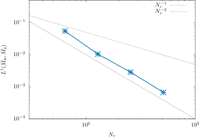
Figure 14: $L^{1}$-norm of the error in the mass accretion rate, for the benchmark test presented in Sec. V.1. The test is performed using the radial resolutions $N_{r}=64,128,256,512$. The black dashed lines represent the expected tendency for a first (top) and second order (bottom) convergence.

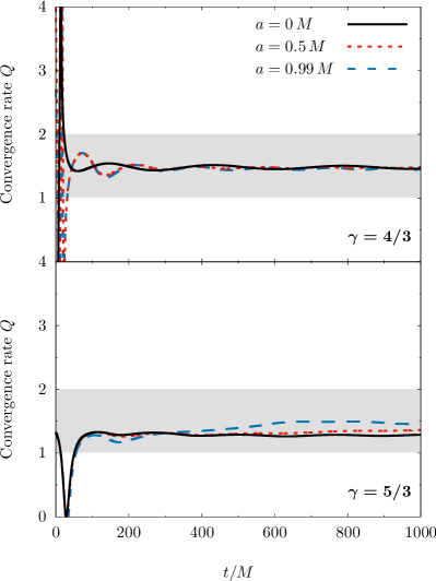
Figure 15: Self-convergence tests of the polytropic fluid simulations, for both values of $\gamma$: 4/3 (top panel) and 5/3 (bottom panel). In this figure we show the evolution in time of the convergence rate $Q$ for three different values of the spin parameter $a$. The gray stripe shows the expected convergence zone (given the numerical methods used in aztekas).

In this appendix we present the convergence and self-convergence tests that are necessary to validate our numerical results.

For the benchmark test presented in Sec. V.1 we compute, for each resolution studied, the relative error between the numerical and analytic values of the mass accretion rate, once the steady state has been reached. In Fig. 14 we present the results of these values as a function of the radial resolution $N_{r}$, from which we obtain second order convergence, as expected for smooth solutions considering the numerical methods used in aztekas.

On the other hand, in order to validate the numerical results of the polytropic fluid simulations reported in Sec. V.2, we perform a series of self-convergence tests in which, using three different consecutive resolutions, we compute the convergence rate of the solution. We carry out the simulations using resolutions $R_{1}=64\times 64$, $R_{2}=128\times 128$, and $R_{3}=256\times 256$, for each studied value of the adiabatic index $\gamma$ and three different values of the spin parameter $a/M=0,\,0.5,\,0.99$.

In Fig. 15 we show the evolution in time of the convergence rate $Q$, which is computed as

$$2^{Q}=\frac{|\dot{M}_{1}-\dot{M}_{2}|}{|\dot{M}_{2}-\dot{M}_{3}|},$$ (116)

where $\dot{M}_{1}$, $\dot{M}_{2}$ and $\dot{M}_{3}$ are the values of the mass accretion rate as obtained from resolutions $R_{1}$, $R_{2}$, and $R_{3}$, respectively. As can be seen from this figure, the time evolution of the simulations’ convergence rate rapidly becomes confined within the gray stripe. Note that in this case, since we have set free-outflow boundary conditions for the velocity field, the simulations develop sharp global oscillations throughout the domain during their evolution, causing the convergence rate to be less than second order, which would have been otherwise expected since we obtain a smooth final steady state solution.

References

- [1] M.A. Abramowicz and P.C. Fragile. Foundations of Black Hole Accretion Disk Theory. Living Reviews in Relativity, 16(1):1, January 2013.
- [2] B. P. Abbott, R. Abbott, T. D. Abbott, and et al. GWTC-1: A Gravitational-Wave Transient Catalog of Compact Binary Mergers Observed by LIGO and Virgo during the First and Second Observing Runs. Phys. Rev. X, 9:031040, Sep 2019.
- [3] The LIGO Scientific Collaboration, the Virgo Collaboration, R. Abbott, T. D. Abbott, S. Abraham, F. Acernese, K. Ackley, A. Adams, C. Adams, R. X. Adhikari, and et al. Population Properties of Compact Objects from the Second LIGO-Virgo Gravitational-Wave Transient Catalog. arXiv e-prints, page arXiv:2010.14533, October 2020.
- [4] Event Horizon Telescope Collaboration. First M87 Event Horizon Telescope Results. I. The Shadow of the Supermassive Black Hole. Astrophysical Journal Letters, 875(1):L1, April 2019.
- [5] H. Bondi. On spherically symmetrical accretion. Monthly Notices Roy Astronom. Soc., 112:195–204, 1952.
- [6] L. Rezzolla and O. Zanotti. Relativistic Hydrodynamics. Oxford University Press, Oxford, 2013.
- [7] F.C. Michel. Accretion of matter by condensed objects. Astrophysics and Space Science, 15:153–160, 1972.
- [8] H. Bondi and F. Hoyle. On the mechanism of accretion by stars. Mon. Not. R. Astron. Soc., 104:273, 1944.
- [9] F. Hoyle and A. Lyttleton. The effect of interstellar matter on climatic variation. Mathematical Proceedings of the Cambridge Philosophical Society, 35:405–415, 7 1939.
- [10] E. Tejeda and A. Aguayo-Ortiz. Relativistic wind accretion on to a Schwarzschild black hole. Mon. Not. R. Astron. Soc., 487(3):3607–3617, August 2019.
- [11] S. Mendoza, E. Tejeda, and E. Nagel. Analytic solutions to the accretion of a rotating finite cloud towards a central object - I. Newtonian approach. Mon. Not. R. Astron. Soc., 393:579–586, February 2009.
- [12] E. Tejeda, S. Mendoza, and J. C. Miller. Analytic solutions to the accretion of a rotating finite cloud towards a central object - II. Schwarzschild space-time. Mon. Not. R. Astron. Soc., 419:1431–1441, January 2012.
- [13] E. Tejeda, P. A. Taylor, and J. C. Miller. An analytic toy model for relativistic accretion in Kerr space-time. Mon. Not. R. Astron. Soc., 429:925–938, February 2013.
- [14] L. Nobili, R. Turolla, and L. Zampieri. Spherical Accretion onto Black Holes: A Complete Analysis of Stationary Solutions. Astrophys. J. , 383:250, December 1991.
- [15] J. Karkowski, B. Kinasiewicz, P. Mach, E. Malec, and Z. Świerczyński. Universality and backreaction in a general-relativistic accretion of steady fluids. Phys. Rev. D, 73(2):021503, January 2006.
- [16] P. Mach and E. Malec. Stability of self-gravitating accreting flows. Phys. Rev. D, 78(12):124016, December 2008.
- [17] P.C. Fragile, A. Gillespie, T. Monahan, M. Rodriguez, and P. Anninos. Numerical Simulations of Optically Thick Accretion onto a Black Hole. I. Spherical Case. Astrophysical Journal Supplement, 201(2):9, August 2012.
- [18] C. Roedig, O. Zanotti, and D. Alic. General relativistic radiation hydrodynamics of accretion flows - II. Treating stiff source terms and exploring physical limitations. Mon. Not. R. Astron. Soc., 426(2):1613–1631, October 2012.
- [19] A. Sadowski, R. Narayan, A. Tchekhovskoy, and Y. Zhu. Semi-implicit scheme for treating radiation under M1 closure in general relativistic conservative fluid dynamics codes. Mon. Not. R. Astron. Soc., 429(4):3533–3550, March 2013.
- [20] J.C. McKinney, A. Tchekhovskoy, A. Sadowski, and R. Narayan. Three-dimensional general relativistic radiation magnetohydrodynamical simulation of super-Eddington accretion, using a new code HARMRAD with M1 closure. Mon. Not. R. Astron. Soc., 441(4):3177–3208, July 2014.
- [21] F.D. Lora-Clavijo, M. Gracia-Linares, and F.S. Guzmán. Horizon growth of supermassive black hole seeds fed with collisional dark matter. Mon. Not. Roy. Astron. Soc., 443:2242–2251, 2014.
- [22] E. Chaverra and O. Sarbach. Radial accretion flows on static, spherically symmetric black holes. Class. Quantum Grav., 32:155006, 2015.
- [23] E. Chaverra, M.D. Morales, and O. Sarbach. Quasi-normal acoustic oscillations in the Michel flow. Phys. Rev. D, 91:104012, 2015.
- [24] L.R. Weih, H. Olivares, and L. Rezzolla. Two-moment scheme for general-relativistic radiation hydrodynamics: a systematic description and new applications. Mon. Not. R. Astron. Soc., 495(2):2285–2304, May 2020.
- [25] R. Hunt. A fluid dynamical study of the accretion process. Mon. Not. R. Astron. Soc., 154:141, January 1971.
- [26] E. Shima, T. Matsuda, H. Takeda, and K. Sawada. Hydrodynamic calculations of axisymmetric accretion flow. Mon. Not. R. Astron. Soc., 217:367–386, November 1985.
- [27] J. A. Font and J. M. Ibáñez. Non-axisymmetric relativistic Bondi-Hoyle accretion on to a Schwarzschild black hole. Mon. Not. R. Astron. Soc., 298:835–846, August 1998.
- [28] M. Ruffert. Three-dimensional Hydrodynamic Bondi-Hoyle Accretion. I. Code Validation and Stationary Accretors. Astrophys. J. , 427:342, May 1994.
- [29] J. A. Font, J. M. Ibáñez, and P. Papadopoulos. Non-axisymmetric relativistic Bondi-Hoyle accretion on to a Kerr black hole. Mon. Not. R. Astron. Soc., 305:920–936, May 1999.
- [30] F. D. Lora-Clavijo and F. S. Guzmán. Axisymmetric Bondi-Hoyle accretion on to a Schwarzschild black hole: shock cone vibrations. Mon. Not. R. Astron. Soc., 429:3144–3154, March 2013.
- [31] L.I. Petrich, S. Shapiro, and S.A. Teukolsky. Accretion onto a moving black hole: An exact solution. Phys. Rev. Lett., 60:1781–1784, 1988.
- [32] X. Hernandez, P. L. Rendón, R. G. Rodríguez-Mota, and A. Capella. A Hydrodynamical Mechanism for Generating Astrophysical Jets. Revista Mexicana de Astronomía y Astrofísica, 50:23–35, April 2014.
- [33] A. Aguayo-Ortiz, E. Tejeda, and X. Hernandez. Choked accretion: from radial infall to bipolar outflows by breaking spherical symmetry. Mon. Not. R. Astron. Soc., 490(4):5078–5087, December 2019.
- [34] E. Tejeda, A. Aguayo-Ortiz, and X. Hernandez. Choked Accretion onto a Schwarzschild Black Hole: A Hydrodynamical Jet-launching Mechanism. Astrophys. J. , 893(1):81, April 2020.
- [35] J.M. Bardeen and J.A. Petterson. The Lense-Thirring Effect and Accretion Disks around Kerr Black Holes. Astrophysical Journal Letters, 195:L65, January 1975.
- [36] M. Liska, A. Tchekhovskoy, A. Ingram, and M. van der Klis. Bardeen-Petterson alignment, jets, and magnetic truncation in GRMHD simulations of tilted thin accretion discs. Mon. Not. R. Astron. Soc., 487(1):550–561, July 2019.
- [37] D. Proga and M. C. Begelman. Accretion of low angular momentum material onto black holes: Two-dimensional hydrodynamical inviscid case. The Astrophysical Journal, 582(1):69–81, Jan 2003.
- [38] P. Mach, M. Piróg, and J. A. Font. Relativistic low angular momentum accretion: long time evolution of hydrodynamical inviscid flows. Classical and Quantum Gravity, 35(9):095005, Mar 2018.
- [39] S. L. Shapiro, A. P. Lightman, and D. M. Eardley. A two-temperature accretion disk model for Cygnus X-1: structure and spectrum. Astrophys. J. , 204:187–199, February 1976.
- [40] F. Yuan and R. Narayan. Hot Accretion Flows Around Black Holes. Annual Review of Astronomy and Astrophysics, 52:529–588, August 2014.
- [41] R. Narayan and I. Yi. Advection-dominated Accretion: A Self-similar Solution. Astrophysical Journal Letters, 428:L13, June 1994.
- [42] R. Narayan and I. Yi. Advection-dominated Accretion: Underfed Black Holes and Neutron Stars. Astrophys. J. , 452:710, October 1995.
- [43] R.D. Blandford and M.C. Begelman. On the fate of gas accreting at a low rate on to a black hole. Mon. Not. R. Astron. Soc., 303(1):L1–L5, February 1999.
- [44] R.D. Blandford and M.C. Begelman. Two-dimensional adiabatic flows on to a black hole - I. Fluid accretion. Mon. Not. R. Astron. Soc., 349(1):68–86, March 2004.
- [45] M.C. Begelman. Radiatively inefficient accretion: breezes, winds and hyperaccretion. Mon. Not. R. Astron. Soc., 420(4):2912–2923, March 2012.
- [46] I. V. Igumenshchev, R. Narayan, and M. A. Abramowicz. Three-dimensional Magnetohydrodynamic Simulations of Radiatively Inefficient Accretion Flows. Astrophys. J. , 592(2):1042–1059, August 2003.
- [47] J.F. Hawley and J.H. Krolik. Magnetically Driven Jets in the Kerr Metric. Astrophysical Journal, 641(1):103–116, April 2006.
- [48] D. Proga. Dynamics of Accretion Flows Irradiated by a Quasar. Astrophysical Journal, 661(2):693–702, June 2007.
- [49] A. Tchekhovskoy, R. Narayan, and J. C. McKinney. Efficient generation of jets from magnetically arrested accretion on a rapidly spinning black hole. Mon. Not. R. Astron. Soc., 418(1):L79–L83, November 2011.
- [50] R. Narayan, A. Sadowski, R. F. Penna, and A. K. Kulkarni. GRMHD simulations of magnetized advection-dominated accretion on a non-spinning black hole: role of outflows. Mon. Not. R. Astron. Soc., 426(4):3241–3259, November 2012.
- [51] T. Waters, A. Aykutalp, D. Proga, J. Johnson, H. Li, and J. Smidt. Outflows from inflows: the nature of Bondi-like accretion. Mon. Not. R. Astron. Soc., 491(1):L76–L80, January 2020.
- [52] C.W. Misner, K.S. Thorne, and J.A. Wheeler. Gravitation. W. H. Freeman, 1973.
- [53] S.W. Hawking and G.F.R. Ellis. The Large Scale Structure of Space Time. Cambridge University Press, Cambridge, 1973.
- [54] Digital library of mathematical functions. http://dlmf.nist.gov/.
- [55] V. Karas and R. Mucha. Accretion onto a rotating compact object in general relativity. American Journal of Physics, 61:825–828, September 1993.
- [56] E. Tejeda. Incompressible Wind Accretion. Revista Mexicana de Astronomía y Astrofísica, 54:171–178, April 2018.
- [57] J.M. Bardeen. A variational principle for rotating stars in general relativity. Astrophys. J., 162:71–95, October 1970.
- [58] J.M. Bardeen. Timelike and null geodesics in the Kerr metric. In C. DeWitt and B.S. DeWitt, editors, Black Holes, Les Astres Occlus, pages 215–239, New York, 1973. Gordon and Breach Science Publishers, Inc.
- [59] A. Aguayo-Ortiz, S. Mendoza, and D. Olvera. A direct Primitive Variable Recovery Scheme for hyperbolic conservative equations: The case of relativistic hydrodynamics. PLoS ONE, 13:e0195494, April 2018.
- [60] F. Banyuls, J.A. Font, J.M. Ibáñez, J.M. Martí, and J.A. Miralles. Numerical 3 + 1 General Relativistic Hydrodynamics: A Local Characteristic Approach. Astrophys. J. , 476(1):221–231, February 1997.
- [61] L. Del Zanna, O. Zanotti, N. Bucciantini, and P. Londrillo. ECHO: a Eulerian conservative high-order scheme for general relativistic magnetohydrodynamics and magnetodynamics. Astronomy and Astrophysics, 473(1):11–30, October 2007.
- [62] C.-W. Shu and S. Osher. Efficient Implementation of Essentially Non-oscillatory Shock-Capturing Schemes. Journal of Computational Physics, 77(2):439–471, August 1988.
- [63] Miguel Alcubierre. Introduction to 3+1 numerical relativity. International series of monographs on physics. Oxford Univ. Press, Oxford, 2008.
- [64] J.D. Jackson. Classical Electrodynamics. John Wiley & Sons, New York, 1975.