Simulating TeV gamma-ray morphologies of shell-type supernova remnants

Abstract

Supernova remnant (SNR) shocks provide favourable sites of cosmic ray (CR) proton acceleration if the local magnetic field direction is quasi-parallel to the shock normal. Using the moving-mesh magneto-hydrodynamical (MHD) code Arepo we present a suite of SNR simulations with CR acceleration in the Sedov-Taylor phase that combine different magnetic field topologies, density distributions with gradients and large-scale fluctuations, and – for our core-collapse SNRs – a multi-phase interstellar medium with dense clumps with a contrast of $10^{4}$. Assuming the hadronic gamma-ray emission model for the TeV gamma-ray emission, we find that large-amplitude density fluctuations of $\delta\rho/\rho_{0}\gtrsim 75$ per cent are required to strongly modulate the gamma-ray emissivity in a straw man’s model in which the acceleration efficiency is independent of magnetic obliquity. However, this causes strong corrugations of the shock surface that are ruled out by gamma-ray observations. By contrast, magnetic obliquity-dependent acceleration can easily explain the observed variance in gamma-ray morphologies ranging from SN1006 (with a homogeneous magnetic field) to Vela Junior and RX J1713 (with a turbulent field) in a single model that derives from plasma particle-in-cell simulations. Our best-fit model for SN1006 has a large-scale density gradient of $\nabla{n}\simeq 0.0034~{}{\rm c}{\rm m}^{-3}~{}{\rm pc}^{-1}$ pointing from south-west to north-east and a magnetic inclination with the plane of the sky of $\lesssim 10^{\circ}$. Our best-fit model for Vela Junior and RX J1713 adopts a combination of turbulent magnetic field and dense clumps to explain their TeV gamma-ray morphologies and moderate shock corrugations.

1 Introduction

Ions are believed to be accelerated to relativistic energies at astrophysical shocks, which gives rise to the observed CR population in the Galaxy (Hillas 2005, Blasi 2013 for a review). In particular, the process of diffusive shock acceleration (Axford et al., 1977; Krymskii, 1977; Blandford & Ostriker, 1978; Bell, 1978a, b) enables particles to gain energy through multiple shock crossings as they scatter back and forth on magnetic field irregularities. The emerging non-thermal spectrum follows a universal power-law momentum spectrum (Bell, 1978a; Blandford & Ostriker, 1978). Supernova explosions and subsequently formed remnant shocks are considered to be ideal environments for acceleration because of the large spatial extent and lifetime that provides sufficient confinement to reaching high energies (Ghavamian et al., 2013; Neronov, 2017). The most energetic CRs are able to escape upstream the shock and propagate to larger distances in the interstellar medium (ISM) while less energetic CRs are advected downstream and only released at a later time (Bell et al., 2013).

Evidence for efficient acceleration of CR electrons is provided by the observation of elongated but narrow X-ray synchrotron filaments that are aligned with the shock surface such as in Tycho (Hwang et al., 2002; Warren et al., 2005; Cassam-Chenaï et al., 2007), Vela Jr. (Bamba et al., 2005), or SN1006 (Bamba et al., 2003; Katsuda et al., 2010), see also Parizot et al. (2006) for an overview. Modelling the emission requires fast electron synchrotron losses in a strongly amplified magnetic field in the upstream (Morlino et al., 2010, for the case of SN1006), which is likely realised through the non-resonant hybrid instability (Bell, 2004; Caprioli & Spitkovsky, 2014b), providing indirect evidence for efficient proton acceleration. This evidence is further strengthened by multi-wavelength analyses that take into account the SNR evolution, hydrodynamics of the shock (assuming spherical symmetry), magnetic field amplification and the dynamical backreaction of CRs and self-generated magnetic turbulence on the shock (Berezhko et al., 2003; Zirakashvili & Aharonian, 2010; Morlino & Caprioli, 2012). The total density jump as measured from far upstream to the downstream exceeds the canonical limit of four (for an ideal gas with adiabatic index 5/3) due to the increased compressibility of the additional relativistic pressure of CRs (Chevalier, 1983; Castro et al., 2011; Caprioli & Spitkovsky, 2014a; Pfrommer et al., 2017). This implies a smaller distance between the contact discontinuity (CD) and the forward shock (FS) as observed in Tycho (Warren et al., 2005) as well as in SN1006 (Cassam-Chenaï et al., 2008), where this CD-FS distance shows a distinctive azimuthal variation such that it is shorter in the polar cap regions, which show efficient amplification of the magnetic field due to efficient CR proton acceleration (in part, the CD-FS distance is reduced by the Rayleigh-Taylor instability of the CD).

Of particular interest is the very high energy (VHE) gamma-ray emission from SNRs in the GeV and TeV regimes (Hillas, 2005), which directly probes the CR component without the need to model the magnetic field. Exceptional examples are shell-type SNRs, such as SN1006, Vela Jr. and RX J1713-3948.5 (RX J1713 for short). Gamma-ray emission associated with these objects can be produced in two different models (Gabici & Aharonian, 2016; Marcowith et al., 2016). In the hadronic model $\pi^{0}$ mesons are produced in inelastic CR-gas interactions and decay into pairs of gamma rays (Caprioli, 2011). In the leptonic model the gamma-ray radiation arises from a combination of inverse Compton scattering of the cosmic microwave background (CMB) and starlight photons off of the accelerated CR electrons and non-thermal bremsstrahlung. Following the CR electron spectrum in three-dimensional MHD simulations of SNRs and modelling the multi-frequency spectrum and emission maps from the radio to gamma-rays suggests that the GeV gamma-ray regime has a significant leptonic contribution while the TeV range is dominated by hadronic gamma rays (Winner et al., 2020).

The leptonic model naturally produces hard gamma-ray spectra while such a spectrum can also be obtained in the hadronic model when considering a clumpy ISM. Magnetic insulation of these dense clumps only allows high-energy CR protons to penetrate into the dense regions, which implies a substantial hardening of the proton spectrum in comparison to the acceleration spectrum in the diffuse ISM (Gabici & Aharonian, 2014; Celli et al., 2019). Combining synchrotron and inverse Compton fluxes in the leptonic model produces volume-filling magnetic field strengths of $\approx(10-35)\,\mu$G (Gabici & Aharonian, 2016; Winner et al., 2020). These are only in agreement with mG-field strengths inferred from X-ray synchrotron filaments when assuming a clumpy medium, arguing for a detailed study of SNR emission maps. By contrast, many previous studies focused on matching the multi-frequency spectra with spherically symmetric models of the SNR evolution and neglecting the diversity of morphological appearances of the observed shell-type SNRs.

In fact, the orientation of the upstream magnetic field plays an important role in the acceleration process. Self consistent hybrid particle-in-cell (PIC) simulations show that a quasi-parallel configuration is much more efficient in accelerating CR protons in comparison to a quasi-perpendicular shock geometry (Caprioli & Spitkovsky, 2014a; Caprioli et al., 2015). These PIC simulations also show that the normalisation of the non-thermal spectrum decreases with time (Caprioli & Spitkovsky, 2014b), which keeps the energy in the non-thermal tail saturated despite the linear increase of the maximum CR particle energy with time (Caprioli & Spitkovsky, 2014c) so that the maximum acceleration efficiency of CR protons at quasi-parallel shocks is limited to $\approx 15$ per cent (Caprioli & Spitkovsky, 2014a). The idea that the resulting emission could depend on the direction of the magnetic field in the X-ray band has also been discussed (Rothenflug et al., 2004). In our previous papers (Pais et al., 2018, 2020; Winner et al., 2020), we find that the global topology of the magnetic field is fundamental in reproducing the diversity of observed gamma-ray emission that ranges from a bi-lobed to a patchy morphology. While an approximately homogeneous magnetic field produces a bi-lobed gamma-ray emission, a turbulent field manifests itself in a patchy emission characteristics. In this scenario, gamma-ray bright regions result from quasi-parallel shocks which are known to efficiently accelerate CR protons, and gamma-ray dark regions point to quasi-perpendicular shock configurations. In the case of an extremely small magnetic correlation length the emission approaches an isotropic emission, albeit with a reduced effective acceleration efficiency (Pais et al., 2018).

The interaction of a supernova explosion with a gas cloud has been explored in various works (Chevalier, 1974; Korolev et al., 2015) and more recently with highly-evolved individual explosions (Zhang & Chevalier, 2019). In particular, interstellar turbulence and its effect on CR acceleration (Scalo & Elmegreen, 2004) has been the subject of various studies in the past years (Elmegreen & Scalo 2004 for a review). Simulations of single SNe have been performed in an inhomogeneous ISM (Walch & Naab, 2015) as well as in the presence of a clumpy circumstellar medium (Obergaulinger et al., 2014; Pais et al., 2020). The clumpiness of the medium is often assumed to be the sole source of irregularity of the emission morphology, especially for strongly asymmetric distributions of heavy elements like Si and Fe in the surroundings of SNRs as confirmed by XMM-Newton measurements (Li et al., 2015).

Following the spirit of this work, we simulate how an inhomogeneous medium affects and regulates the TeV gamma-ray morphology of SNRs in the Sedov-Taylor phase. We perform our simulations with various magnetic field configurations combined with magnetic obliquity-dependent shock acceleration. In order to infer morphological properties of the ambient medium of observed SNRs, we compare the resulting emission maps, radial and azimuthal profiles with three well-known examples of shell-type SNRs such as SN1006, Vela Jr. and RX J1713. For simplicity we use an initial setup of a point explosion that evolves into the Sedov-Taylor solution. The gamma-ray emission from the resulting SNR is then computed using a hadronic model of decaying pions. Our goal is to find a consistent model that simultaneously explains the detailed gamma-ray spectrum as well as the morphological variance of the TeV gamma-ray emission maps.

This paper is organised as follows. In Section 2 we present the methodology used to prepare our initial conditions for the various models with particular focus on the generation of an initial turbulent density and magnetic field. In Section 3 we present our suite of SNR simulations with different combinations of magnetic fields (homogeneous and turbulent) and density distributions (homogeneous, with a gradient, turbulent and a combination of a gradient and turbulence), yielding a wide range of different morphologies. For comparison, we also test a straw man’s model of an isotropic acceleration scenario (i.e., independent of magnetic obliquity). In Section 4 we compare the observed gamma-ray map, radial and azimuthal profiles of SN1006 with our simulations for different degrees of turbulence and inclinations of the field of view and infer properties on the local ISM. In Section 5 we compare radial and azimuthal profiles of turbulent SNRs Vela Jr. and RX J1713 to the models with a turbulent magnetic field and a non-obliquity dependent acceleration for various density setups. In Section 6, we study the effect of strong density fluctuations on the gamma-ray morphology of a core-collapse SNR in its early Sedov stage. In Section 7, we show that we can match the gamma-ray spectra of all three SNRs for our adopted parameters and summarise the main findings and conclude in Section 8.

2 Methodology

Here we present our methodology and briefly explain the procedure used to implement obliquity dependent CR acceleration, the turbulence in the ISM and in the initial magnetic field. Results of this setup are shown in Section 3.

2.1 Simulation method

The simulations presented in this paper are performed with the massively parallel, adaptive moving mesh-code Arepo (Springel, 2010). We use an improved second-order hydrodynamic scheme with the least squares-fit gradient estimate and a Runge-Kutta time integration (Pakmor et al., 2016). Ideal MHD is used to model the magnetic fields (Pakmor & Springel, 2013) while zero-divergence is enforced through the implementation of a Powell scheme (Powell et al., 1999). CRs are modelled as a relativistic fluid with a constant relativistic adiabatic index of 4/3 in a two-fluid approximation (Pfrommer et al., 2017).

Shocks are localised and characterised using the method developed by Schaal & Springel (2015), where Voronoi cells that exhibit a maximally converging velocity field along the direction of propagation of the shock are selected, while spurious shocks and numerical noise are filtered out. We inject CR energy into the Voronoi cells in the immediate post-shock regime of shock above a critical Mach number of $\mathcal{M}>3$ (Pfrommer et al., 2017).

Following the results of hybrid PIC simulations performed in Caprioli & Spitkovsky (2014a) we assume a maximum CR energy efficiency of $15$ per cent for quasi-parallel shocks. On the contrary quasi-perpendicular shocks are found to be extremely inefficient accelerators. We note that the value of the maximum CR energy efficiency is uncertain. Arguments involving the Galactic CR energy budget to match the power needed to sustain the observed Galactic CR intensity favour average acceleration efficiencies of 3 to 10 per cent (Drury et al., 1989; Aharonian et al., 2006b; O’C. Drury, 2014; Kroll et al., 2015), which can be scaled to maximum CR acceleration efficiencies at quasi-parallel shocks of 10 to 30 per cent (Pais et al., 2018), thus bracketing our value of 15 per cent. The efficiency of the accelerated CRs is computed using the orientation of the pre-shock upstream magnetic field (Pais et al., 2018).

The presence of a strong current associated with streaming CRs into the upstream region causes an exponential growth of the magnetic fluctuations via the non-resonant hybrid instability (Bell, 2004). These amplified fluctuations saturate at wave amplitudes corresponding to the strength of the mean magnetic field and cause the CR scattering mean free path to decrease to values comparable with the fluctuating gyroradius. This regime approaches the Bohm limit of diffusion. On scales resolved by our simulations, we neglect CR diffusion and streaming. To justify this approach we assume Bohm diffusion and calculate the CR precursor length for SNRs considered in this work and find

$$L_{{\rm prec}} \sim\sqrt{\kappa_{\rm Bohm}t_{\rm age}}\simeq$$ (1)

$$\simeq 0.3~{}{\rm pc}\left(\dfrac{\langle pc\rangle}{10~{}{\rm T}{\rm eV}}\right)^{1/2}\left(\dfrac{B}{10\mu{\rm G}}\right)^{-1/2}\left(\dfrac{t_{\rm age}}{10^{3}{\rm yr}}\right)^{1/2},$$

where $\langle pc\rangle$ is the average energy associated with the protons that emit TeV gamma rays through the inelastic proton-proton reaction, $B$ is the root-mean-square of the upstream magnetic field and $t_{\rm age}$ is the age of the remnant. The resulting precursor length is below the size of our numerical resolution $\Delta x=0.4~{}{\rm pc}$, assuming a simulation box size of $40~{}{\rm pc}$ that is filled with $100^{3}$ cells. Energy losses of accelerated CRs escaping upstream from the blast wave do not affect the validity of the self-similar solution of the problem, causing only a negligible softening of the Sedov-Taylor solution (Bell, 2015). On the SNR timescales simulated, the hadronic and Coulomb loss time scales are negligibly small so that we only account for adiabatic CR losses.

2.2 Initial conditions

By analogy with Pais et al. (2018), we start with a random Voronoi mesh that is regularised into a glass-like configuration via Lloyd’s algorithm (Lloyd, 1982). We inject the equivalent of $E_{\mathrm{SN}}=10^{51}{\rm erg}$ of thermal energy in the central cell of a $100^{3}$-cell periodic box with a side length of $L=40~{}{\rm pc}$. The resulting explosion forms an energy-driven strong shock expanding in an ISM characterised by a low pressure of $0.44~{}{\rm eV}~{}{\rm c}{\rm m}^{-3}$, and a mean molecular weight of $\mu=1.4$.

2.2.1 Magnetic field setup

To generate a turbulent magnetic field we follow the procedure by Ruszkowski et al. (2017) and Pais et al. (2018). We adopt a Kolmogorov-like power spectrum for the magnetic field and generate the three magnetic vector components independently in Fourier space such that the resulting field exhibits a random phase. We ensure that $\boldsymbol{B}$ is divergence-free by projecting out the radial field component in Fourier space. The degree of turbulence is determined through the fraction $f_{B}$ of magnetic energy which goes into turbulent modes, yielding

$$B_{\rm tot}^{2}=B_{0}^{2}+B_{\rm turb}^{2}$$ (2)

where $B_{0}^{2}=B_{\rm tot}^{2}(1-f_{B})$ represents the strength of the mean field, $B_{\rm turb}^{2}=\langle\delta\boldsymbol{b}^{2}\rangle=f_{B}B_{\rm tot}^{2}$ is the average value of the Gaussian random field, and $\delta\boldsymbol{b}(\boldsymbol{x})$ is the local value of the turbulent field at the coordinates $\boldsymbol{x}=(x,y,z)$. Note that $0\leq f_{B}\leq 1$ where $f_{B}=0$ corresponds to a fully homogeneous field and $f_{B}=1$ corresponds to a fully turbulent field. We adopt a plasma beta factor of $\beta=1$ such that the magnetic and thermal pressures are insignificant in comparison to the kinetic energy of the propagating shock front. To maintain hydrostatic equilibrium in the initial conditions, magnetic fluctuations $\delta\boldsymbol{B}(\boldsymbol{x})$ are compensated by adopting temperature fluctuations of the form $nk_{B}\delta T(\boldsymbol{x})=-\delta\boldsymbol{B}^{2}(\boldsymbol{x})/(8\pi)$. The small magnetic field strength implies a small Alfvén speed so that the tension force is only slowly mediated and does not affect the dynamics of our powerful shock wave.

2.2.2 ISM density setup

We model the multiphase structure of the ISM and adopt a combination of (i) a large-scale linear density gradient, (ii) large-scale turbulent density fluctuations that follow a Kolmogorov spectrum, and (iii) a population of small, dense gaseous clumps with a typical overdensity of $10^{4}$ in comparison to the ambient ISM.

The large-scale density gradient $\rho_{\mathrm{grad}}$ is determined by the constant density $\rho_{0}$ and the slope parameter $\Delta$. Similarly to the magnetic field, we generate turbulent density fluctuations in Fourier space and vary the initial seed, the correlation length and the amplitude of fluctuations $\rho_{\mathrm{turb}}(\boldsymbol{x})=\rho_{0}\delta\rho(\boldsymbol{x})$. To avoid negative values for the density we adopt a density floor of $10^{-2}\rho_{0}$. All these elements are combined as follows:

$$\rho(\boldsymbol{x})= \rho_{0}+\rho_{\mathrm{turb}}(\boldsymbol{x})+\rho_{\mathrm{grad}}(\boldsymbol{x})=\rho_{0}\left[1+\delta\rho(\boldsymbol{x})\right]$$

$$+\rho_{2}\left[\left(\frac{x}{L}-\frac{1}{2}\right)\cos\psi+\left(\frac{y}{L}-\frac{1}{2}\right)\sin\psi\right],$$ (3)

where $L$ is the side length of our simulation box, $\psi$ represents the angle between the direction of the density gradient and the $x-$axis, $\delta\rho(\boldsymbol{x})$ is the generating functional of the turbulent field, $\rho_{2}=\sqrt{2}\Delta\rho_{0}/(1+\Delta)$ is the amplitude of the gradient such that $\rho=\rho_{0}(1+\rho_{0}\delta\rho)$ for $\Delta=0$ in case of a vanishing gradient. The function $\rho_{\mathrm{grad}}(\boldsymbol{x})$ is constructed such that there are no negative values for the density in the simulation box for any $x,y\in[0,L]$ and $\Delta\in[0,\infty)$. To avoid low-density cavities in the surroundings of the central explosion, we shield the region with a constant homogeneous density of $\rho=\rho_{0}$ extending for a radius of $2~{}{\rm pc}$.

In order to reliably model the circum-stellar medium of our core-collapse SNRs, we include a population of dense gaseous clumps with a typical size of 0.1 pc and a number density of $\sim 10^{3}{\rm c}{\rm m}^{-3}$ (Inoue et al., 2012). Following the general setup as in Pais et al. (2020) and Celli et al. (2019), we include $7\times 10^{3}$ uniformly distributed small, dense clumps with a number density of $n_{\mathrm{c}}=10^{3}~{}{\rm c}{\rm m}^{-3}$ and a diameter of $0.1~{}{\rm pc}$ of a total target mass of $M_{\mathrm{c}}=45M_{\odot}$ engulfed by the shock. Because of the quasi-Lagrangian property of our moving mesh code Arepo, we resolve each small clump with initially 1000 cells that are uniformly distributed within the spherical clump volumes. As shown in Appendix A of Pais et al. (2020), our simulations accurately follow the dynamics of and inside every dense cloud that is site of vorticity generation upon the passage of the shock wave. As a result, Kelvin-Helmholtz instabilities start to mix cold, dense cloud material with the ambient hot shocked gas, which causes the formation of dense, ram-pressure stripped tails in the wake of each cloud (see figure 2 of Pais et al., 2020).

This flexible setup allows us to study a wide range of different situations and environments by modifying the amplitude of the density fluctuations, their coherence scale and steepness of the gradient as well as their multi-phase nature of thermally unstable dense clumps in the star-forming surroundings of core-collapse SNRs.

2.3 Modelling gamma-ray emission and noise

To model the gamma-ray emission in post-processing we assume that the CR population follows a universal power law momentum spectrum. A pion-decay hadronic model is used to calculate the omni-directional gamma-ray emissivity (Pfrommer & Enßlin, 2004; Pfrommer et al., 2008) which depends on the local ISM density, the local CR population, the very-high energy (i.e. $>1~{}{\rm T}{\rm eV}$) photon spectral index $\alpha_{\gamma}$, and the energy range.

To compute the emission spectra of our simulations we integrate a particle population described by a power law in momenta with cutoff. The hadronic gamma-ray emission spectrum is calculated from parametrizations of the cross section of neutral pion production at low and high proton energies, respectively (Yang et al., 2018; Kelner et al., 2006).

In order to match the morphological properties of the observed gamma-ray emission maps we proceed with an analysis of the power spectrum of the noise. We fit the power spectrum with a specific function, convert it into a noise map. This noise map is then superposed on the mock gamma-ray emission map that was convolved with the observational point spread function (PSF). We will detail the method to generate the noise properties in Section 4.

Figure 1: Impact of inhomogeneities density and magnetic field on the gamma-ray maps of SNRs in the Sedov-Taylor phase at $t_{\mathrm{age}}=10^{3}{\rm yr}$ with side length $L=40~{}{\rm pc}$. The images are ordered according to their different initial conditions: the magnetic field configurations and acceleration models differ between the three columns, and the adopted density distributions are different horizontally between each row. The first two columns assume magnetic obliquity dependent CR acceleration at a homogeneous magnetic field (left) and a fully turbulent fluctuations of relative amplitude $f_{B}=1$ and coherence length $\lambda_{B}=20~{}{\rm pc}$ (middle) while the third column shows simulations with a turbulent field ($\lambda_{\rho}=20~{}{\rm pc}$) but with an isotropic CR acceleration model. We adopt the following density distribution for all three simulations in each row: constant density (first row), an increasing gradient pointing from SW to NE (second row), turbulent density fluctuation (third row) and a combination of turbulence and a gradient (fourth row). The arrows indicate the direction of the magnetic field and the density gradient (if present).

3 Exploring fluctuations in density and the magnetic field

Using the previously described setup here we present a suite of twelve SNR simulations (each with $100^{3}$ cells) and combine different topologies of the magnetic field and different density distributions. We also compare models of obliquity-dependent CR acceleration to isotropic CR acceleration. The gamma-ray emission maps in the energy range $1-80$ TeV with a spectral index of $\alpha=2.1$ are shown in Fig. 1 at a SNR age of $t=1000$ yrs. The images are not convolved with a PSF and we do not add noise in order to maintain the underlying setup as transparent as possible.

For these theoretical models we chose a simple setup both for the density and the magnetic field. We start by separately considering the components of the density distribution of Eqn. (3). For the background density we select a value of $n=0.1~{}{\rm c}{\rm m}^{-3}$. The density gradient has an inclination of $\psi=135^{\circ}$ with respect to the $x$-axis, i.e., it is pointing from south-west (SW) to north-east (NE) and exhibits a moderate gradient intensity of $\Delta=1$ to avoid a strong contrast between the upper-left quadrant and the bottom-right one. For the turbulence we chose turbulent fluctuations of $f_{\rho}=\delta\rho/\rho_{0}=0.5$ and a coherence scale of $\lambda_{\rho}=L/2$ for our box size $L=40~{}{\rm pc}$. To avoid any correlation between magnetic and density fluctuations in our turbulent simulations, we used two distinct but fixed random seeds, respectively.

3.1 Density fluctuations

In the first column of Fig. 1 we show the models for a constant magnetic field oriented with an angle of $\theta=135^{\circ}$ with respect to the positive $x$-axis. The effect of the obliquity-dependent shock acceleration in presence of an ordered magnetic field is manifested in the bi-lobed morphology of the gamma-ray emission. The presence of a moderate gradient in the second and fourth row results in NE lobe brighter than the SW lobe as expected in the presence of more ISM material on which the shock impinges so that the freshly accelerated CR protons find more target gas in a hadronic scenario.

3.2 Magnetic turbulence

In the central column of Fig. 1 we show the effect of a fully turbulent magnetic field ($f_{B}=1$) that is superposed on different density distributions. As expected, the obliquity-dependent shock acceleration allows the creation of a patchy distribution of the brightness echoing the distribution of the underlying locally accelerated CR population (Pais et al., 2020). In particular, the combination with a turbulent density distribution (Fig. 1, third row, centre) is responsible for a noticeable modulation of the gamma-ray intensity and explains the bright spot in the lower right corner close to the remnant shell, an absent feature in the constant density map (Fig. 1, first row, centre).

As expected in an isotropic acceleration scenario (Fig. 1, right column) the gamma-ray emissivity shines along the entire SNR shell and is only mildly modulated by local or large-scale variations related to the particular density distribution used in the simulation. Contrarily to the obliquity-dependent case for turbulent fields depicted in the central column, a considerable amount of emission is still present in the centre of the remnant.

For isotropic models the emission in the centre is at least twice as strong as the turbulent case. This is caused by the efficient CR acceleration in the isotropic model so that the emission is projected onto the central parts of the SNR. By contrast, in the obliquity-dependent scenario for the turbulent magnetic case we obtain a patchy structured emission with bright spots in regions with a quasi-parallel shock geometry and dark regions in locally quasi-parallel shocks geometries. On average the acceleration process for medium to large scale turbulence is $70$ per cent less efficient with respect to the non obliquity dependent case (Pais et al., 2018). This results in a stronger dispersion of the brightness and a lower average absolute emissivity in the centre. Note that observational noise and the presence of a population of cold-dense clumps in a multi-phase ISM may play an important role and needs to be taken in consideration for the morphological modelling of observed shell-type SNRs.

Table 1: Comparison of simulation and observational parameters for the presented hadronic morphological models.

	SN1006		Vela Jr.		RX J1713
Parameter	Simulation	Observed	Simulation	Observed	Simulation	Observed
diameter $\theta_{\mathrm{s}}$ [deg]	0.5	0.5	2	2	1	1
$D$ [kpc]	1.79	1.45 $-$ 2.2	0.5	$0.2-0.75$	1	$0.5-1$
diameter $d_{\mathrm{s}}$ [pc]	15.6	12.6 $-$19.2	17.4	$7.0-26.1$	17.4	$8.7-17.4$
$t_{\rm age}$ [kyr]	1	1	$2.7$	$2.4-5.1$	$3$	$1-7.9$
$E_{\mathrm{SN}}~{}$[$10^{51}$ erg]	1	$-$	1	$-$	1	$-$
density $n~{}[{\rm c}{\rm m}^{-3}]$	0.1	0.05 $-$ 0.3	0.42	$0.03-1$	$0.57$	$0.02-1$
$\nabla n~{}[{\rm c}{\rm m}^{-3}{\rm pc}^{-1}]$	0.0034	$-$	$-$	$-$	$0.02$	$-$
$M_{\mathrm{c}}~{}[M_{\odot}]$	$-$	$-$	45	$-$	45	$-$
$\langle v_{\mathrm{s}}\rangle~{}[{\rm k}{\rm m}~{}{\rm s}^{-1}]$	3000	$2100-4980$	2000	$>1000-3000$	1100	$800-3900$
$\mathcal{F}_{\gamma}(>1\mathrm{TeV})~{}[10^{-12}\mathrm{ph}~{}\mathrm{cm}^{-2}~{}\mathrm{s}^{-1}]$	0.4	$0.39\pm 0.08$	24	$23.4\pm 5.6$	16.3	$16.3\pm 0.2$
$\alpha_{\mathrm{p},\mathrm{e}}$	1.95	$1.79\pm 0.44$	1.81	$1.85\pm 0.24$	1.7	$1.52\pm 0.31$
$E_{\mathrm{p},\mathrm{cut}}[{\rm T}{\rm eV}]$	200	$-$	100	$-$	90	$-$
$E_{\mathrm{e},\mathrm{cut}}[{\rm T}{\rm eV}]$	$1.7$	$-$	$0.25$	$-$	$0.25$
$\beta_{\mathrm{p}}$	2	$-$	2	$-$	2	$-$
$\beta_{\mathrm{e}}$	0.7	$-$	0.4	$-$	0.4	$-$
References	1, 2, 6, 8, 9, 10, 13, 21		2, 3, 4, 8, 10, 14, 16, 17, 19		5, 7, 8, 11, 12, 15, 19, 20

Notes: $n$ denotes the diffuse ISM number density, $\nabla n$ is the large-scale density gradient, $M_{\mathrm{c}}$ is the target clump mass hit by the remnant, $D$ is the distance to the SNR, $\theta_{\mathrm{s}}$ and $d_{\mathrm{s}}$ are the angular and proper extent of the blast wave, $\langle v_{\mathrm{s}}\rangle$ denotes the shock velocity, $t_{\rm age}$ is the SNR age and $\mathcal{F}_{\gamma}$ is the integrated gamma-ray flux above 1 TeV. References: (1) Acero et al. (2007) ; (2) Acero et al. (2015); (3) Allen et al. (2015); (4) Aschenbach et al. (1999); (5) Celli et al. (2019); (6) Dubner et al. (2002); (7) Federici et al. (2015); (8) Green (2014); (9) H.E.S.S. Collaboration (2010); (10) H.E.S.S. Collaboration (2018b); (11) H.E.S.S. Collaboration (2018a); (12) Inoue et al. (2012); (13) Katsuda et al. (2008); (14) Katsuda (2017); (15) Leahy et al. (2020); (16) Ming et al. (2019); (17) Slane et al. (2001); (18) Takahashi et al. (2008) (19) Tanaka et al. (2011); (20) Tsuji & Uchiyama (2016); (21) Winkler et al. (2003).

It is clear that the isotropic acceleration model fails to reproduce both the emission morphologies (lobes and filaments) and the strong azimuthal variation in the emission of SN1006. Despite a significantly varying amplitude of density fluctuations of 50 per cent, the azimuthal variation in the isotropic-acceleration runs does not drop sufficiently to create clearly defined filamentous structures in the shell. High-amplitude turbulence in the ISM on scales comparable to the size of the remnant might be a solution and could potentially mimic a bi-lobed structure. We will come back to this point in Section 6 and will show that the almost spherically symmetric blast waves of the SNRs studied here put a strong constraint on the level of large-scale inhomogeneity of the surrounding ISM.

Figure 2: Left: Comparison of the noise power spectra of the observed emission map of SN1006 (H.E.S.S. Collaboration, 2010) with the signal regions masked and of the simulated gamma-ray map of SN1006 with a turbulent density fraction of $\delta\rho/\rho_{0}=0$. This shows that our modelled noise nicely corresponds to the observed noise properties. Right: Sketch of the area used for calculating the azimuthal and the radial profiles of the simulated models. We average the gamma-ray emission in the radial range $2/3<r/\langle r_{\mathrm{s}}\rangle<4/3$ to obtain the azimuthal profile while the lobe regions are used to compute the radial profiles for SN1006.

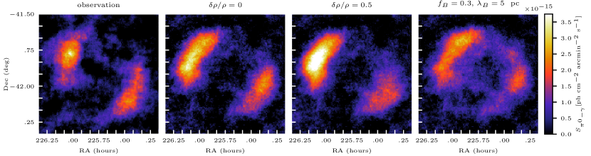
Figure 3: Two-dimensional projected gamma-ray maps for SNR SN1006 and for three simulation models with a fixed density gradient and different amplitudes of turbulent density fluctuations. The second and third panels show the simulated maps for $f_{\rho}=5~{}{\rm pc}$ and $\delta\rho/\rho=0$ and $0.5$, respectively, while the rightmost panel shows the map for $f_{B}=0.3$, $\lambda_{B}=5~{}{\rm pc}$ and $\delta\rho/\rho=0$. The emission in the simulated maps is smoothed with a Gaussian PSF of width $\sigma=0.045^{\circ}$. On the top of it, we add Gaussian noise with the power spectrum inferred from HESS data, as shown in Fig. 2, at fixed random seed.

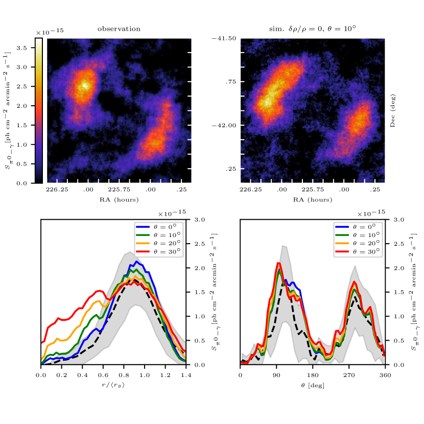
Figure 4: Top left: emission map of SN1006 (H.E.S.S. Collaboration, 2010). Top right: our best match for SN1006 without density fluctuations and a rotation angle $\theta=10^{\circ}$. Bottom left: radial profiles of the surface brightness. Profiles of the best match for $\theta=[0^{\circ},10^{\circ},20^{\circ},30^{\circ}]$ are reported for comparison with the observed one (black dashed line). The grey-filled areas represent the standard deviations of the observed radial profiles, respectively. The more strongly inclined cases ($\theta=20^{\circ}$ and $\theta=30^{\circ}$) fail to reproduce the declining emission inside and outside the maximum. Bottom right: Comparison of simulated azimuthal profiles of SN1006 and observed data (black dashed line) with standard deviation (grey). While there is broad agreement between the models and observation, the NE cap (at around 90^∘) is narrower in the HESS observation.

4 Morphological modelling of SN 1006

In the following two sections, we use our intuition developed in our parameter study in Fig. 1 to find the most promising combination of magnetic and density inhomogeneities in the obliquity-dependent acceleration scenario to mock the observed gamma-ray emission morphology of shell-type SNRs. To this end, we analyse the bi-lobed morphology of Type Ia SN1006 in this section and present our analysis of the two shell-type core-collapse SNRs Vela Jr. and RX J1713 in Section 5.

The gamma-ray excess map of SN1006 reported by the H.E.S.S. Collaboration (2010) strongly correlates with the synchrotron X-ray emission map and suggests an emitting region compatible with a thin shell. The peculiar polar cap geometry in the emission is also observed in other wavelengths such synchrotron X-ray emission, indicating an acceleration process compatible with efficient quasi-parallel shock acceleration (Winner et al., 2020). Polarimetric radio observations of the limbs strongly suggests that the ambient field is aligned along the SE–NW direction (Reynoso et al., 2013), as later confirmed by recent theoretical models (Schneiter et al., 2015). Moreover in Pais et al. (2020) is shown that the correlation length of the magnetic field in case of pure turbulence is at least 15 times the angular size of the SNR and consistent with a homogeneous field across the SNR.

All these models used a setup involving a homogeneous ISM. However, if the TeV gamma-ray emission is mainly from hadronic sources, the brighter NE lobe suggests the presence of a large scale density gradient pointing from SW to NE. Furthermore, the small-scale brightness variations at the outer shock radius could either be caused by (i) density inhomogeneities in the ISM that would corrugate the shock upon colliding with these inhomogeneous structures or (ii) by obliquity-dependent shock acceleration in combination with small-scale turbulent magnetic field superposed on a homogeneous magnetic field. We will study the impact of both effects on the gamma-ray surface brightness maps in the presence of a large-scale density gradient.

4.1 Simulation model

We proceed with a suite of simulations with the same large-scale density gradient but with different setups for the density and magnetic field topology. We conducted a number of exploratory simulations to test the steepness of the gradient in order to faithfully reproduce the different TeV gamma-ray brightness of the two lobes and match the measured fluxes reported in H.E.S.S. Collaboration (2010). For the average value of the density and SNR distance we used the same values reported by the Pais et al. (2020). With reference to Eq. 3 we used $\psi=135^{\circ}$ for the orientation and $\Delta=0.9$ for the density slope. In physical units this corresponds to a density gradient of $\nabla n\simeq 0.0034~{}{\rm c}{\rm m}^{-3}~{}{\rm pc}^{-1}$ pointing from SW to NE, which means that in the NE region the average ISM density is $\langle n\rangle\sim 0.12~{}{\rm c}{\rm m}^{-3}$ while in the SW rim we find $\langle n\rangle\sim 0.08~{}{\rm c}{\rm m}^{-3}$. Initially, we adopt a homogeneous magnetic field 5 $\mu{\rm G}$ throughout the simulation domain.

Our baseline model does not adopt turbulent density and magnetic fluctuations. Our second model assumes turbulent density fluctuations with a amplitude $\delta\rho/\rho\sim 0.5$ and coherence scale $\lambda_{\rho}=5~{}{\rm pc}$. Finally, our third model has no turbulent density fluctuations, but adopts magnetic turbulence with $f_{B}\sim 0.3$ and coherence scale $\lambda_{B}=5~{}{\rm pc}$. We simulated and evolved our SN1006 model for $1010$ yrs, constructed the pion-decay gamma-ray surface brightness map resulting from hadronic CR interactions and convolved it to the observational PSF of width $\sigma=R_{68}/1.515=0.042^{\circ}$, with $R_{68}=0.064^{\circ}$ (H.E.S.S. Collaboration, 2010). All other parameters used for the simulations are reported in Table 1.

4.2 Noise modelling

In order to disentangle physical effects that generate small-scale brightness fluctuations from spurious instrumental effects, we need to accurately model the instrumental noise. This noise dominates the lower excess counts and is normally distributed with zero mean. Here, we explain our procedure of generating such a noise map for our synthetic gamma-ray emission maps. To this end, we calculate the noise power spectrum of the excess map of SN1006 and exclude the emission of the NE and SW lobes. This is done by masking the original excess map from the H.E.S.S. Collaboration (2010) with a sharp cutoff equal to $c_{\mathrm{cut}}=|c_{\mathrm{min}}|$ where $c_{\mathrm{min}}=-20$ is the minimum value of the excess counts of the H.E.S.S. observations of SN1006. This procedure is justified by the fact that the noise excess counts follow a normal distribution with zero mean (see Appendix A).

The power spectrum of SN 1006 is obtained via a 2D Fourier transform of the masked data set. The noise power spectrum presents two features: (i) a large scale Gaussian-like noise as expected from the PSF convolution of the instrument, and (ii) a small scale power law $\propto k^{-2}$ extending to higher modes. We fit the power spectrum with the following function in $k$-space:

$$P(k)=A\exp\left(-\dfrac{k^{2}}{2\sigma^{2}_{k}}\right)+Bk^{-2}$$ (4)

where, $\sigma_{k}$ represents the standard deviation in $k$-space and the variables A and B determine the relative strength of the Gaussian and the power-law tail. The black dashed line in Fig. 2 shows the measured noise power spectrum of the SN1006 excess map in comparison to the simulated noise (blue line). We assume that the noise is fully characterised by two-point correlations and obtain a random realisation of the noise via 2D inverse Fourier transform. This noise map is then superposed on the mock gamma-ray emission map that was convolved with the observational point spread function (PSF).

4.3 Simulated TeV emission

We show the resulting synthetic maps of SN 1006 in comparison to the original excess map in Fig. 3. We report three gradient models with the following assumptions (from left to right): (i) no density fluctuations, (ii) density fluctuations with $\delta\rho/\rho=0.5$ and no magnetic field fluctuations, and (iii) magnetic field fluctuations with $\delta B/B=0.3$ and no density inhomogeneities. This enables us to separately analyse the effect of these configurations on the morphology of SN1006.

While our noise modelling is responsible for emission in regions where the acceleration is supposed to be extremely inefficient or absent, the density perturbations are able to corrugate and smooth the boundaries of the lobes, in particular of the SW lobe for the chosen seed. The resulting picture appears with a defined bi-lobed structure and an increasing level of turbulence in the medium causes the emergence of secondary morphological details. We notice that density perturbation of $\delta\rho/\rho=0.5$ (third picture of Fig. 3) affect the morphology of the SW lobe resulting in a fainter surface brightness and a broader shape. This suggests that our preferred model for SN 1006 in the TeV gamma-ray band is given by a model with homogeneous density.

Similarly, we observe the emergence of secondary morphological details from a moderate level of turbulence in the magnetic field (fourth picture of Fig. 3) in our obliquity dependent CR acceleration scenario. We compare this model with a coherence scale at $\sim 1/3$ the size of the remnant to our other two models with a homogeneous density and a moderate level of density inhomogeneities. In spite of the low level of magnetic fluctuations ($\delta B/B=0.3$) the morphology significantly deviates from the observed bi-lobed shell-type morphology of SN1006 and shows significant substructures. In addition, this model is also ruled out by the excess of the emission in the central region of the remnant which contrasts to the clean separation of the two lobes as observed by the H.E.S.S. collaboration. This sets an approximate upper limit for the local turbulence of the magnetic field in a obliquity dependent scenario.

Another degree of freedom is the orientation of the homogeneous magnetic field $\boldsymbol{B}_{0}$ with respect to the line of sight. To study its influence on the emission map and (radial and azimuthal) profiles, we perform a three-dimensional (3D) rotation of the SNR around the axis perpendicular to the orientation of $\boldsymbol{B}_{0}$ into the line of sight. We show different inclinations ($\theta=[0^{\circ},10^{\circ},20^{\circ},30^{\circ}]$) of $\boldsymbol{B}_{0}$ with respect to the plane of the sky, similarly to Bocchino et al. (2011) for the X-ray emission to constrain the 3D orientation of the magnetic field of SN 1006. Note that this is somewhat degenerate with the assumed 3D orientation of the density gradient that we also assume to lie in the plane of the sky.

An increasing inclination results in a less pronounced peak and a broader distribution of gamma rays as the hadronic emission from the efficiently accelerated CRs at the quasi-parallel shocks changes from being limb-brightened to contributing to a broader solid angle on the sky. The top right panel in Fig. 4 shows our best match for SN1006 after the aforementioned rotation of the SNR. Indeed, the lobes appear slightly more diffuse, predominantly in the internal regions.

To quantify the effect of magnetic inclination we compute the radial and azimuthal profiles of our synthetic maps according to the sketch shown on the right-hand side of Fig. 2. The radial profiles are computed within the quadrants where quasi-parallel shock acceleration takes place while the azimuthal profiles show an average in the radial range $2/3<r/\langle r_{\mathrm{s}}\rangle<4/3$, where $r_{\mathrm{s}}$ is the average shock radius of the SNR.

The comparison of the post-rotation radial profiles to the observed radial profile of SN 1006 provides an important constraint for the maximum magnetic inclination. These profiles are show in the bottom panels of Fig. 4. We include a $1\sigma$ standard deviation grey-filled area to the observed SN1006 profiles. While larger inclinations ($\theta>10^{\circ}$, orange and red lines) result in emission profiles that are too extended, an inclination of $\theta\leq 10^{\circ}$ is in better agreement with the observed radial profile. Barring our remark about the orientation of the density gradient, we conclude that the magnetic inclination does not exceed $10^{\circ}$ with respect to the plane of the sky.

A minor element of discordance can be also found in the azimuthal profiles (Fig. 4, bottom right) for different rotation angles. While the simulated SW lobes coincide with the observed one in relative brightness and extension, the simulated NE lobe is slightly broader in comparison to the observed lobe. This suggests that the critical angle for the magnetic obliquity may be smaller than $45^{\circ}$ inferred by recent PIC simulations. Regardless the spatial rotation all the models reproduce the observed modulation of the two lobes within the 1-$\sigma$ uncertainty.

5 Morphological modelling of core collapse SNRs

We now turn to two other well-known SNRs with a clear shell-type morphology: Vela Jr. and RX J1713. Both SNRs are of core-collapse origin which means that the ambient ISM is a star-forming region of multi-phase, turbulent gas. We account for this by simulating the supernova explosion in a multiphase ISM with a large population of small, dense gaseous clumps with a typical overdensity of $10^{4}$ in comparison to the ambient ISM and adopt a purely turbulent magnetic field without a mean field, $\boldsymbol{B}_{0}=\mathbf{0}$.

5.1 Observational constraints on Vela Jr.

The H.E.S.S. Collaboration (2018b) has observed TeV gamma-ray emission from the SNR Vela Jr. (RX-J0852.0-4622) with a resolved gamma-ray spectrum. Estimates on the SNR age vary from a very young remnant of $\sim 700$ yrs (Aschenbach et al., 1999) to an older object of more than 5000 yrs (Katsuda et al., 2008). The SNR can be a nearby object at $D=0.2~{}{\rm k}{\rm pc}$, as inferred from studies of the decay of ${}^{44}\mathrm{Ti}$ nuclei (Iyudin et al., 1998), or a more distant one at $D=0.75~{}{\rm k}{\rm pc}$, as inferred from the slow expansion of X-ray filaments (Katsuda et al., 2008). The presence of interstellar molecular clouds suggests that the origin of TeV-gamma rays from these objects is mainly hadronic (Fukui, 2013).

The lack of thermal X-ray emission places a very low limit at $n=0.03~{}{\rm c}{\rm m}^{-3}$ while assuming a homogeneous environmental density (Slane et al., 2001). However, if the ISM is composed of dense clumps that are embedded in a lower-density hot ambient phase, the resulting thermal X-ray emission (of the hot phase) is lower while the presence of the dense clumps implies a higher average density. A conventional approach in the hadronic model is to use a density of the order of $n\sim 1~{}{\rm c}{\rm m}^{-3}$ (Aharonian et al., 2006a), while hydrodynamic models suggest values of less than $0.4~{}{\rm c}{\rm m}^{-3}$ (Allen et al., 2015). More recently HI and CO measurements and partial morphological correspondence with the TeV-gamma ray morphology indirectly suggest an extremely high average ISM density of the order of $n\sim 100~{}{\rm c}{\rm m}^{-3}$ (Fukui et al., 2017). However there is no direct observational evidence that the clumped gas is in direct physical contact with the shock-accelerated cosmic rays. In fact the passage of the shock dissipates kinetic energy, heats the ions to particle energies of several keV and is directly responsible of dissociation of CO and $\mathrm{H}_{2}$ and the ionisation of the neutral part of the clouds on a time-scale of the order of a few years (Celli et al., 2019).

As the shock overruns the magnetised ISM, magnetic fields are draped around the dense clouds, precluding the diffusion of cosmic rays deep into the cloud so that the TeV cosmic rays can only probe a narrow skin of the cloud. The penetration depth of this skin can be estimated by realising that the draped magnetic field reaches strength of order $B\approx\sqrt{8\pi\alpha\rho v^{2}}\approx 1\mathrm{mG}$ (Dursi & Pfrommer, 2008; Pfrommer & Dursi, 2010) for typical parameters $\alpha=2$, $n=0.1~{}{\rm c}{\rm m}^{-3}$, and $v_{\mathrm{s}}=3000~{}{\rm k}{\rm m}~{}{\rm s}^{-1}$. If the average ISM density were indeed $100~{}{\rm c}{\rm m}^{-3}$ (Fukui et al., 2017), this should yield draped magnetic field strengths of 32 mG, which should be observable via Zeeman splitting of which there is no evidence which argues against such a high average density. The skin depth of the dense cloud reachable by TeV CRs, assuming Bohm diffusion, varies from a few to several gyro radii:

$$r_{g}=\dfrac{p_{\perp}c}{eB}\approx 10^{-6}~{}{\rm pc}\left(\dfrac{pc}{{\rm T}{\rm eV}}\right)\left(\dfrac{B}{{\rm m}{\rm G}}\right)^{-1}$$ (5)

which is negligible in comparison of the cloud size (0.1 pc). Even if the magnetic wrap is not perfect and CRs can penetrate 100 gyro radii inside the cloud, then the fraction of the cloud volume seen by the TeV CRs is $\Delta V\sim 1-(1-10^{-3})^{3}\sim 3\times 10^{-3}$. Our assumed total dense cloud mass of $45~{}\mathrm{M}_{\odot}$ that is physically associated with the SNR is a fraction of $2\times 10^{-3}$ of the available gas mass of $2.5\times 10^{4}~{}\mathrm{M}_{\odot}$ (Fukui et al., 2017) towards the Vela Jr. region, some of which may be projected onto the SNR but is not physically associated to it and only a tiny fraction of the molecular and neutral gas inside the Vela Jr. SNR is seen by cosmic rays due to magnetic draping, suppressing cosmic ray propagation into the cloud before the cold gas gets ionised and dissociated. These considerations justify our assumption of only accounting for CR advection in our simulations.

In addition, not all the mass of the clumps engulfed by the shock has been processed by the shock because of the strong deceleration of the blast wave inside the clumps (see Appendix of Pais et al. 2020). Combining these arguments suggests that only a tiny fraction of the dense (neutral/molecular) phase of the ISM is in physical contact with the shock. For the magnetic field we decided to follow the same prescription used in Pais et al. (2020) setting the coherence scale of the turbulent magnetic field to $\lambda_{B}=13~{}{\rm pc}$ and adopt $f_{B}=1$. The entire set of parameters used in the simulation is summarised in Table 1.

5.2 Observational constraints on RX J1713

RX J1713 represents another bright TeV-emitter with a distinct shell-like emission morphology. This SNR is subject to intense studies thanks to its strong non-thermal X-ray emission and the detection of high-energy and very-high-energy gamma-rays. Wang et al. (1997) suggested that RX J1713 is linked to an AD393 guest star which, according to historical records, appeared in the tail of constellation Scorpius, close to the actual position of the remnant. This would put the age of the remnant close to $1.6~{}{\rm k}{\rm yr}$. More recent estimates based on X-ray emission combined with hydro models in homogeneous media suggest an older remnant age of $6.8^{+1.1}_{-2}{\rm k}{\rm yr}$ (Leahy et al., 2020).

The distance of the object is estimated to be around $1~{}{\rm k}{\rm pc}$ (Fukui et al., 2003) while Tanaka et al. (2008) suggests a distance interval between 0.5 kpc and 1 kpc. Assuming a free expansion model this translates into an upper limit of the average shock speed of about $\langle v_{\mathrm{s}}\rangle=6300~{}{\rm k}{\rm m}~{}{\rm s}^{-1}$. Proper motions of bright X-ray filaments instead place the shock velocity between $\sim 1000~{}{\rm k}{\rm m}~{}{\rm s}^{-1}$ and $\sim 4000~{}{\rm k}{\rm m}~{}{\rm s}^{-1}$ (Fukui et al., 2003).

A hadronic origin of the TeV gamma-ray emission in RX J1713 was suggested in several papers (Zirakashvili & Aharonian, 2010; Gabici & Aharonian, 2014). The distribution of gas in RX J1713 is crucial to establish the origin of the observed gamma-rays. An upper limit for the diffuse density of $<2~{}{\rm c}{\rm m}^{-3}$ is derived from non thermal X-rays measurements (Takahashi et al., 2008). To explain the lack of thermal X-ray emission Cassam-Chenaï et al. (2004) sets an even lower upper limit for the ambient density of $n\sim 0.02~{}{\rm c}{\rm m}^{-3}$. However, this argumentation can be circumvented by introducing a densely clumped environment.

Studies of non-thermal X-ray emission, TeV gamma-ray emission and their partial spatial correlation with HI ans H2 suggest the presence of numerous dense clumps in the ISM (Fukui et al., 2003; Sano et al., 2015; Rowell et al., 2009). However the same argument used for Vela Jr. applies: the lack of direct evidence of physical contact between the gas distribution and the shock and the subsequent ionisation of HI casts doubts on its physical association with the SNR. The interaction of a blast wave with interstellar clouds and its application to RX J1713 has been studied in Inoue et al. (2012) and applied in Celli et al. (2019) for a shock wave with constant velocity interacting with a target mass of $45~{}M_{\odot}$.

Recently, Tsuji & Uchiyama (2016) calculated the evolution of RX J1713 in various scenarios such as the case of an expansion in a wind-blown cavity with a typical density profile $\rho\propto r^{-2}$ and a free expansion dominated by the ejecta ($\rho_{\mathrm{ej}}\propto r^{-n}$ with $n=7$). Here we consider simple Sedov-Taylor expansion models which represent the upper limit for the expansion of a SNR in homogeneous media (Truelove & McKee, 1999).

To reproduce the saturated NW rim of the remnant we applied a homogeneous positive large-scale gradient to the initial conditions pointing from SE to NW with $\Delta=1.6$, corresponding to a density gradient of $\nabla n=0.02~{}{\rm c}{\rm m}^{-3}~{}{\rm pc}^{-1}$. Superposed on this density gradient we insert a population of dense clumps of size $0.1~{}{\rm pc}$ using exactly the same setup as for Vela Jr. For the magnetic field we selected a fully turbulent setup ($f_{B}=1$) with a coherence length of $\lambda_{B}=13~{}{\rm pc}$, not too dissimilar from the size of the remnant ($\sim 17.4~{}{\rm pc}$). The entire set of parameters used in the simulation is summarised in Table 1.

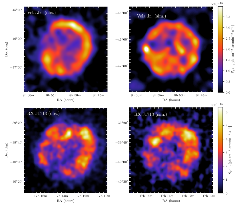
Figure 5: Comparison between observed gamma-ray emission maps (left) of Vela Jr. (H.E.S.S. Collaboration, 2018b) and RX J1713 (H.E.S.S. Collaboration, 2018a) and simulated gamma-ray maps (right) of the SNRs for our model with obliquity-dependent CR acceleration, a turbulent magnetic field with $f_{B}=1$ and $\lambda_{B}=13$ and additionally a gradient for RX J1713 with $\Delta=1.6$. In our simulated maps we add Gaussian noise with the observed power spectrum and use the PSFs appropriate to each observation ($0.08^{\circ}$ and $0.036^{\circ}$ for Vela Jr. and RX J1713, respectively). We also rotated mock emission maps of the SNRs to match the azimuthal position of the faintest region in the shell.

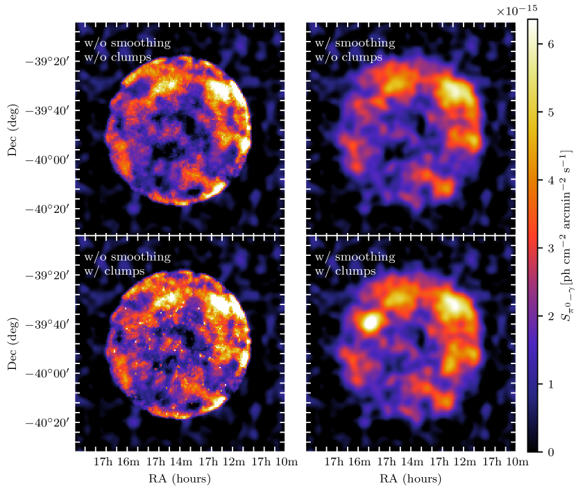
Figure 6: Comparison between the simulated surface brightness maps of RX J1713 without clumps (top row) and with clumps (bottom row). The comparison between the maps without (left) and with PSF smoothing (right) shows the contribution of the clumps in specific portions of the outer shell and in the central region. While most of the gamma-ray substructure is due to obliquity-dependent CR acceleration, individual bright patches in the map can be due to the hadronic emission of dense clumps.

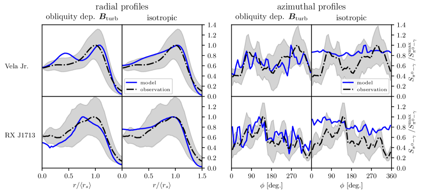
Figure 7: Normalised radial (left-hand side) and angular (right-hand side) profiles of the models (blue lines) shown in Fig. 5 compared to SNRs Vela Jr. (dashed dotted lines in the top row, H.E.S.S. Collaboration 2018b) and RX J1713 (dashed dotted lines in the bottom row, H.E.S.S. Collaboration 2018a). The grey-filled area represents the $1\sigma$ uncertainty for both SNRs. The column labelled with “obliquity dep. $\boldsymbol{B}_{\mathrm{turb}}$” shows our obliquity-dependent acceleration models for a turbulent magnetic field while the label “isotropic” refers to our isotropic acceleration model. While both models reproduce the radial emission profiles well, the isotropic model clearly fails to capture the azimuthal brightness variations seen in the data which is statistically consistent with our obliquity-dependent acceleration model.

5.3 Simulations

Figure 5 shows the comparison between the observed excess brightness maps of Vela Jr. and RX J1713 (left-hand side) and our PSF-convolved synthetic maps derived from turbulent models with density inhomogeneities and dense clumps (right-hand side). To model the noise in the post-processing we applied the same method used for SN1006. In the final step we rotate the surface brightness maps in order to approximately match the low and high emissivity outer shell regions of the observed maps. Our simulation models provide a good agreement with the data.

The presence of high-density molecular clumps provides an important contribution to the global emission morphology. The effect of the clumps on RX J1713 is shown in Fig. 6. While we notice that the orientation of the magnetic field is mainly responsible of the patchy morphology of the outer shell the clumps add several bright spots to the map without modifying the expansion history of the SNR due to their negligible volume filling factor. A comparison with the left-hand side figure in the bottom row shows that the strong smoothing applied to the synthetic maps makes it impossible to resolve the emission originating from a single isolated clump and that clusters of bright clumps are similar to large magnetic field patches oriented quasi-parallel to the shock normal, thus enabling efficient CR acceleration.

The effect of obliquity-dependent shock acceleration is better shown in Fig. 7, where we compare radial and azimuthal profiles of our simulated gamma-ray maps to those of the excess maps of Vela Jr. and RX J1713. We consider the two cases of (i) obliquity-dependent shock acceleration in a turbulent magnetic field and (ii) isotropic CR acceleration, both for a constant ambient density and and global density gradient. While the pure isotropic models (without clumps and PSF smoothing) show and enhance level of surface brightness in the central region compared to the obliquity dependent acceleration models (see Fig. 1), the inclusion of dense clumps and convolution with the observational PSF fills in the central parts to similar emission levels.

Most notably, the isotropic acceleration models cannot reproduce the observed azimuthal small-scale variations in the surface brightness as shown in the right-hand panels of Fig. 7. Interestingly, obliquity-dependent acceleration models are able to modulate the emissivity peaks on a relatively small scale, in a statistically similar fashion. This is a clear prediction of an obliquity-dependent CR acceleration in a turbulently magnetised ISM, in which the morphology of the magnetic field, in tandem with emission from dense clumps, is responsible for the VHE emission morphology observed by imaging air Cerenkov telescope such as H.E.S.S. and enables us to infer the magnetic coherence scale of the ISM surrounding the SNR (Pais et al., 2020). We will address the interesting question whether large-amplitude density perturbations or extreme density gradients alone are able to modulate the surface brightness in a similar way to mimic the VHE observations in Section 6.

6 The case of a highly turbulent medium

Here we study the effect of strong density fluctuations on a supernova explosion in its early Sedov stage at $t_{\rm age}=1~{}{\rm k}{\rm yr}$. We aim at answering two questions: (i) Can high-amplitude turbulence in the ISM on scales comparable to or smaller than the size of the remnant mimic a bi-lobed or patchy VHE gamma-ray emission with strong, small-scale brightness variations observed in the three SNRs studied here and (ii) can localised strong variations of the density be responsible for an extreme corrugation of the shock front and its eventual disruption into smaller clumps, speeding up the end of the Sedov phase, thus anticipating the beginning of the snowplough phase and the eventual merging of the fragments with the ISM? This dynamical effect may feedback on the acceleration mechanism of CRs.

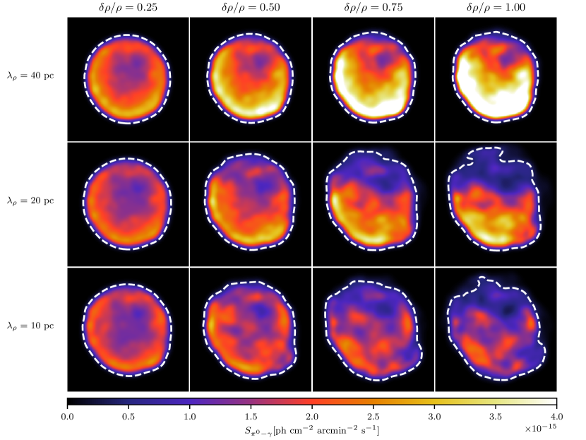
Figure 8: Gamma-ray emissivity from SNRs in the Sedov-Taylor phase with large-amplitude density fluctuations in our isotropic acceleration scenario that does not depend on magnetic obliquity. From left to right the fluctuation strength increases from 0.25 to 1 with respect to the average density in steps of 0.25. From top to bottom the correlation length for the density fluctuations are, in decreasing order: 40 pc (top row), 20 pc (middle row) and 10 pc (bottom row). The maps are taken at $t_{\mathrm{age}}=10^{3}$ yrs after the explosion and all exhibit the same average number density of $0.1~{}{\rm c}{\rm m}^{-3}$. The maps have a side length of $L=20~{}{\rm pc}$ and are smoothed with the PSF of RX J1713 with $\sigma=0.036^{\circ}$. The dashed white curves denote the emission contours used in the histograms of Fig. 9 to quantify the degree of corrugation of the outer shell boundary of the gamma-ray emission.

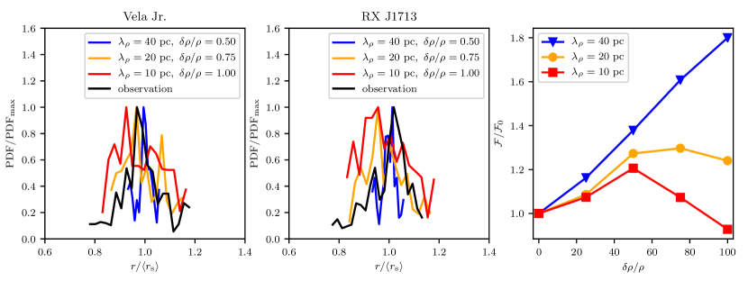
Figure 9: Left and centre: distribution of the radii of the external signal contours of the gamma-ray brightness map shown in white in Fig. 8 for three selected models in our isotropic acceleration scenario that does not depend on magnetic obliquity. Increasing fluctuation amplitude and correlation length implies a larger dispersion of the radial distribution of the outer gamma-ray emission contour and a significant departure from spherical symmetry. For comparison we show the radial distribution of the SNRs Vela Jr.(left) and RX J1713 (centre). Right: Gamma-ray flux of the models pictured in Fig. 8 as a function of the amplitude of density fluctuations. The flux is normalised to the flux $\mathcal{F}_{0}$ of the model without density turbulence. The plot shows an excess emission associated with the coherence length $\lambda_{\rho}=40~{}$pc which grows with increasing degree of turbulence.

In order to test whether our core-collapse SNRs necessarily require an obliquity-dependent acceleration model, we adopt our isotropic CR acceleration model and systematically vary density fluctuations. To this end, we present a set of 12 simulations with varying amplitude of turbulence from $\delta\rho/\rho=0.25$ to $\delta\rho/\rho=1$ at steps of $0.25$, and varying coherence scale of the fluctuations at steps of $L/n$ with box size $L=40~{}{\rm pc}$ and $n=[1,2,4]$. We use the same setup as in our previous models, which is described in Section 2, and show results for the exact same random seed in Fig. 8. From left to right we present an increasing turbulent amplitude while the coherence scale of turbulence decreases from $40$ to $10~{}{\rm pc}$ from top to bottom.

We can clearly see that the shock becomes more corrugated for decreasing coherence scale while increasing the fluctuation amplitude at constant coherence scale has a comparably smaller impact on the azimuthal dependence of the shock propagation speed. We notice that a coherence length of about the size of the remnant or smaller has a strong impact on the corrugation of the outer shell. In particular, the cases of $\lambda_{\rho}=10~{}{\rm pc}$ and $\delta\rho/\rho\geq 0.75$ (two bottom right panels of Fig. 8) show a disruption of the shock front at two locations corresponding to extremely under-dense regions. The breaking of the shell corresponds also to a lower global gamma-ray surface brightness, signalling that less material is accelerated and that eventually the shock escapes detection in that region.

Hence the appearance of a bi-lobed structure as in SN1006 would require extreme fine-tuning of the density distribution which clearly rules out this isotropic CR acceleration scenario in this case. Our parameter study presented in Fig. 8 shows that in order to obtain significant surface brightness variations as is observed in the core-collapse SNRs RX J1713 and Vela Jr., the level of density fluctuations needs to be significant, with $\delta\rho/\rho\gtrsim 0.75$. However, this implies a heavily corrugated shock surface which appears to be in conflict with the overall spherical appearance of SNRs RX J1713 and Vela Jr.

This observation is separately quantified for both SNRs by computing the histogram of the radii of the external signal contours of the TeV gamma-ray emission maps (see Fig. 8). First, we identify the centroid of the SNRs and—in the case of the observations—exclude the background noise. We then determine the external emission contour for both remnants by choosing a threshold of 10 per cent of the maximum excess counts. We show the histogram of these radii, normalised by an average radius $\langle r_{\mathrm{s}}\rangle$ for both remnants, respectively, in Fig. 9. We compare those observed radial emission profiles to the profiles of our simulation model (assuming isotropic CR acceleration) for $\lambda_{\rho}=40~{}{\rm pc}$ with $\delta\rho/\rho=0.5$ (blue line), for $\lambda_{\rho}=20~{}{\rm pc}$ with $\delta\rho/\rho=0.75$ (orange line), and for $\lambda_{\rho}=10~{}{\rm pc}$ with $\delta\rho/\rho=1$ (red line). While large scale fluctuations with $\lambda_{\rho}=40~{}{\rm pc}$ show a moderate dispersion despite the high level of density fluctuations, the models with $\lambda_{\rho}\leq 20~{}{\rm pc}$ are not compatible with the well defined radial dispersion of Vela Jr. and RX J1713. This allows to constrain the level of large-scale density fluctuations to be less than $75$ per cent and $\lambda_{\rho}>20~{}{\rm pc}$. The resulting gamma-ray patchiness is thus not any more strong enough to explain the small-scale gamma-ray brightness variations observed in the SNRs RX J1713 and Vela Jr., which thus rules out this isotropic CR acceleration scenario in these SNRs as well and favours the obliquity-dependent CR acceleration scenario in all shell-type SNRs studied.

The maps with a high level of turbulence and a small coherence scale have a fainter surface brightness. To quantify the lower gamma-ray efficiency of small-scale highly turbulent SNRs, we show the fluxes of our 16 models as a function of the degree of turbulence and of the coherence scale in the right-hand panel of Fig. 9. We find a striking increase in flux with increase turbulent amplitude for our model with $\lambda_{\rho}=40~{}{\rm pc}$. On the contrary for $\lambda_{\rho}\leq 20~{}$pc the opposite is true. In order to check whether this is due to a particular random realisation of our turbulent density field or a systematic effect, we simulate the case of $\lambda_{\rho}=40~{}{\rm pc}$ with $\delta\rho/\rho=[0.5,0.75,1]$ with three different random realisation of turbulence and show the results in Fig. 10. The different monotonic and non-monotonic behaviour of the gamma-ray flux for each random realisation indicates that this behaviour is not systematic and due to random variance.

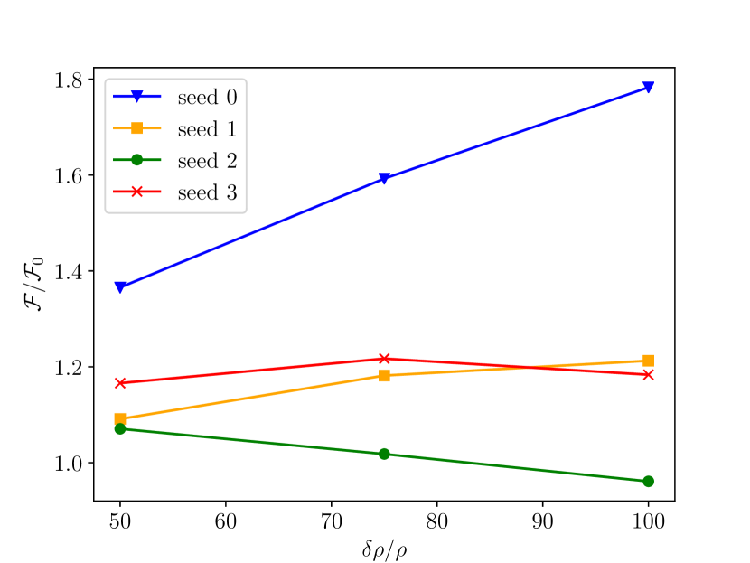
Figure 10: Gamma-ray flux for our turbulent density distribution with $\lambda_{\rho}=40~{}{\rm pc}$ for different random realisations of turbulence as function of the turbulent amplitude. The seed labelled with 0 represents the one used for the realisations in Fig. 8. The plot shows no clear trend associated with the turbulent amplitude. Random seed 0 causes a larger gamma-ray intensity because of the specifics of the overdensities which lead to the formation of a bright shell while this effect is not significant for the other tested random seeds.

7 Spectra

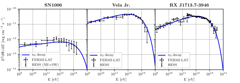
Figure 11: High energy spectra spectra of SN1006 (left), Vela Jr. (centre) and RX J1713 (right). The models assume a hadronic pion-decay emission scenario for the three SNRs. For SN1006, we use data from FERMI (Abdo et al., 2010) and H.E.S.S. (H.E.S.S. Collaboration, 2010) (sum of the two regions). For Vela Jr., we adopt gamma-ray data from FERMI (Tanaka et al., 2011) and H.E.S.S. (H.E.S.S. Collaboration, 2018b). For RX J1713, the gamma-ray data are taken from FERMI (Abdo et al., 2011) and H.E.S.S. (H.E.S.S. Collaboration, 2018a).

Recent observations of the ambient density around Vela Jr. and RX J1713 suggest the presence of clumps and thus a hadronic origin of the GeV-TeV gamma-ray emission (Fukui et al., 2003, 2012; Maxted et al., 2012, 2018). On the other hand, the low density of the dilute phase of ISM and X-ray measurements for SN1006 suggest mixed leptonic-hadronic models to explain both the GeV and the TeV flux in a unified picture as shown by recent simulations (Winner et al., 2020): while the GeV gamma-ray regime has a significant leptonic contribution, in this model the TeV range is dominated by hadronic gamma rays (H.E.S.S. Collaboration, 2010).

We can reproduce the observed VHE gamma-ray spectra of all three SNRs for our adopted parameters. To demonstrate this, we compare the observational data from FERMI and H.E.S.S. to a one-zone model in which the CR proton spectrum is described by a power law with exponential cutoff of the form:

$$f^{\mathrm{1D}}(p)=\dfrac{\mathrm{d}^{2}N}{\mathrm{d}p\mathrm{d}V}\propto p^{-\alpha}\exp\left[-\left(\dfrac{p}{p_{\mathrm{cut}}}\right)^{\beta}\right]$$ (6)

where $f^{\mathrm{1D}}(p)=4\pi\,p^{2}f^{\mathrm{3D}}(p)$, $\alpha$ is the spectral index, $p_{\mathrm{cut}}$ is the cutoff momentum and $\beta$ describes the sharpness of the cutoff; with values reported in Table 1.

The resulting spectra of our hadronic models are shown in Fig. 11 and match the observed spectra. We further notice that in SN1006 the gamma-ray spectrum extends to higher energies, arguing for a larger maximum CR proton energy in comparison to the turbulent cases of Vela Jr. and RX J1713. This difference depends on a range of different factors such the progenitor (SNIa for SN1006 and core-collapse for Vela Jr. and RX J1713), the ISM density, the local magnetic field amplification in the upstream and the time the particles spent in favourable conditions (e.g., quasi-parallel shock geometries) at the shock. However, the limited angular resolution of H.E.S.S. precludes a more in-depth analysis of the acceleration mechanism leaving this task to the next generation of ground-based arrays such the Cherenkov Telescope.

8 Conclusions

In this paper we use MHD simulations with CR physics to explore the effect of density inhomogeneities on the ${\rm T}{\rm eV}$ gamma-ray morphology from SNRs during their Sedov-Taylor stage. Our setup allow us to explore several combinations of homogeneous and turbulent magnetic fields and ambient density distributions. We find that a single physical model, namely obliquity-dependent shock acceleration of CRs, is capable of explaining the apparently disparate TeV gamma-ray morphologies of well-known shell-type SNRs. In this hadronic emission scenario, gamma-ray bright regions result from quasi-parallel shocks which are known to efficiently accelerate CR protons, and gamma-ray dark regions point to quasi-perpendicular shock configurations.

The main characteristics of the emission of SN1006 (a type Ia SN) can be explained by a homogeneous magnetic field superposed on a density gradient that explains the different integrated gamma-ray flux of both polar caps. By contrast, the irregular gamma-ray morphologies of the core collapse SNRs Vela Jr. and RX J1713 is owing to a turbulent magnetic field with $\boldsymbol{B}_{0}\approx\mathbf{0}$ that is supplemented with a population of multiphase dense molecular clumps that are characteristic for star formation regions (and complemented with a weak density gradient in the case of RX J1713). Adapting a straw man’s model of isotropic CR acceleration (that does not depend on magnetic pre-shock orientation) we conclude that this model is not able to reproduce the sharp bi-lobed morphology observed for SN1006 even the presence of moderately strong density fluctuations. Moreover, the simulated azimuthal profiles of this isotropic acceleration model with strong density variations cannot reproduce the observed rapid variations of the gamma-ray emissivity of Vela Jr. and RX J1713 without significantly corrugating the shock surface, which is then ruled out by the spherical morphologies of these SNRs.

Our main findings are summarised here:

• Moderate density fluctuations can be responsible for a local modulation of the gamma-ray emissivity irrespective of the magnetic morphology both in a constructive and destructive way. We show that density fluctuations on a scale comparable to the size of the remnant and with an amplitude that is stronger than $75$ per cent with respect to the mean ISM density causes a corrugated shock front that generates strong local variations in the shock acceleration efficiency and eventually a very asymmetrical appearance of the gamma-ray SNR.

• For SN1006, using the relative brightness of the NE and SW lobes, we constrain the intensity of the density gradient to be no more than $0.0035~{}{\rm c}{\rm m}^{-3}/{\rm pc}$ and directed from SW to NE. We predict that local density fluctuations with $\lambda_{\rho}\simeq 4~{}{\rm pc}$ and $\delta\rho/\rho=0.5$ are secondary in shaping the morphology of the remnant if compared to a moderate level of turbulence of the local magnetic field with a coherence scale at $1/3$ of the size of the remnant. However, we note that the presence of density fluctuations can explain the strong asymmetry of the distribution of Fe and other heavy elements for this remnant.

• The strong noise level surrounding the SN1006 SNR does not allow more precise constraints on the properties of the surrounding ISM. We conclude that for such level of noise a model with negligible density fluctuations better represents the morphology of SN1006. Performing a 3D rotation of the SNR around the axis perpendicular to the orientation of $\boldsymbol{B}_{0}$ into the line of sight, the emerging radial emission profiles constrain the inclination of the magnetic field to be $\lesssim 10^{\circ}$. Our azimuthal emission profiles for different magnetic inclinations are rather robust and show an excellent agreement with the observational profile except for the NE lobe, which is somewhat broader in our simulations. While this could signal a different functional form of the obliquity dependence of CR acceleration, this conclusion is unfortunately degenerate with density fluctuations that could also cause a sharper gamma-ray peak.

• Our generated gamma-ray mock maps with obliquity-dependent acceleration are capable of reproducing most of the properties observed for Vela Jr. and RX J1713 such the length of the shell filaments, the internal patchy emission, the large-scale gamma-ray bright rims and moderate (small-scale) corrugations at the shock front. The fainter emission at the centre of the remnants expanding in a turbulent magnetic field is compensated by the addition of molecular clumps and superposing noise to the images. By contrast an isotropic CR acceleration scenario fails to reproduce the azimuthal profiles.

• In addition, by considering an isotropic CR acceleration scenario for Vela Jr. and RX J1713 with a varying level of density fluctuations and coherence scales, we exclude strong density fluctuations with a coherence scale comparable to the size of the remnant are responsible for the observed emission morphology. This is because sufficiently strong density fluctuations (that would be needed to explain the significant gamma-ray brightness fluctuations) cause a heavily corrugated shock surface which is in direct conflict with the almost spherical shape of SNRs RX J1713 and Vela Jr. The comparison between the radial dispersions of our simulated mock maps and the excess maps of the SNRs RX J1713 and Vela Jr. enables us to limit the density fluctuations to $\delta\rho/\rho_{0}\lesssim 75$ per cent of the average ISM density.

For the first time, our models are able to match morphological and spectral properties of all known shell-type TeV gamma-ray SNRs. Remarkable improvements in the angular resolution in future surveys (beyond what is achievable by CTA) are needed to resolve the TeV emission from individual molecular clumps which would yield a deeper insight in the structure of the circumstellar ISM.

9 Acknowledgements

We would like to thank Ralf Klessen and Volker Springel for the fruitful comments and suggestions to this work. We thank our anonymous referee for a constructive report that helped to improve the paper. We acknowledge support by the European Research Council under ERC-CoG grant CRAGSMAN-646955.

10 Data availability

The data underlying this article will be shared on reasonable request to the corresponding author.

Appendix A Noise threshold for gamma-ray excess maps

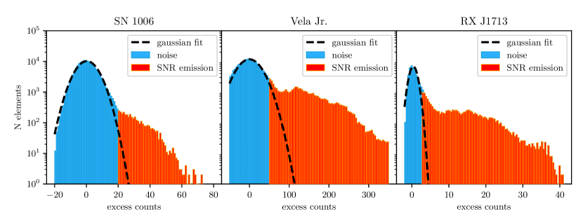
Figure 12: H.E.S.S. gamma-ray excess count distributions of the full gamma-ray brightness maps of SN 1006 (H.E.S.S. Collaboration, 2010), Vela Jr (H.E.S.S. Collaboration, 2018b), and RX J1713 (H.E.S.S. Collaboration, 2018a). The blue parts of the histograms represent the counts associated with noise while the red parts denote excess counts associated with the SNR signal. We fit a normal distribution (black dashed line) with zero mean to show that the significance distribution of the field-of-view is compatible with statistical noise fluctuations.

The gamma-ray excess maps of SN 1006, Vela Jr. and RX-J1713 show detailed signal morphologies in addition to instrumental and gamma-ray reconstruction noise. We assume that the noise is normally distributed and define the noise threshold to be equal to the absolute value of the most negative value. To justify this approach we report the distribution of excess counts of H.E.S.S. observations of the three SNRs analysed here in Fig. 12. This shows that the excess counts at the low end are dominated by Gaussian noise with zero mean. We exclude these counts and isolate the excess counts of the SNR signal. We set $c_{\mathrm{min}}=-20$ for SN 1006, $c_{\mathrm{min}}=-50$ for Vela Jr., and $c_{\mathrm{min}}=-2$ for RX J1713. We note that in our synthetic modeling, the generated noise is also normally distributed with zero mean.

References

- Abdo et al. (2010) Abdo A. A., et al., 2010, ApJS, 188, 405
- Abdo et al. (2011) Abdo et al. A., 2011, ApJ, 734, 28
- Acero et al. (2007) Acero F., Ballet J., Decourchelle A., 2007, A&A, 475, 883
- Acero et al. (2015) Acero F., Lemoine-Goumard M., Renaud M., Ballet J., Hewitt J. W., Rousseau R., Tanaka T., 2015, A&A, 580, A74
- Aharonian et al. (2006a) Aharonian et al. F., 2006a, A&A, 449, 223
- Aharonian et al. (2006b) Aharonian F., et al., 2006b, ApJ, 636, 777
- Allen et al. (2015) Allen G. E., Chow K., DeLaney T., Filipović M. D., Houck J. C., Pannuti T. G., Stage M. D., 2015, ApJ, 798, 82
- Aschenbach et al. (1999) Aschenbach B., Iyudin A. F., Schönfelder V., 1999, A&A, 350, 997
- Axford et al. (1977) Axford W. I., Leer E., Skadron G., 1977, International Cosmic Ray Conference, 11, 132
- Bamba et al. (2003) Bamba A., Yamazaki R., Ueno M., Koyama K., 2003, ApJ, 589, 827
- Bamba et al. (2005) Bamba A., Yamazaki R., Hiraga J. S., 2005, ApJ, 632, 294
- Bell (1978a) Bell A. R., 1978a, MNRAS, 182, 147
- Bell (1978b) Bell A. R., 1978b, MNRAS, 182, 443
- Bell (2004) Bell A. R., 2004, MNRAS, 353, 550
- Bell (2015) Bell A. R., 2015, MNRAS, 447, 2224
- Bell et al. (2013) Bell A. R., Schure K. M., Reville B., Giacinti G., 2013, MNRAS, 431, 415
- Berezhko et al. (2003) Berezhko E. G., Ksenofontov L. T., Völk H. J., 2003, A&A, 412, L11
- Blandford & Ostriker (1978) Blandford R. D., Ostriker J. P., 1978, ApJ, 221, L29
- Blasi (2013) Blasi P., 2013, Astronomy and Astrophysics Review, 21, 70
- Bocchino et al. (2011) Bocchino F., Orlando S., Miceli M., Petruk O., 2011, A&A, 531, A129
- Caprioli (2011) Caprioli D., 2011, Journal of Cosmology and Astro-Particle Physics, 2011, 026
- Caprioli & Spitkovsky (2014a) Caprioli D., Spitkovsky A., 2014a, ApJ, 783, 91
- Caprioli & Spitkovsky (2014b) Caprioli D., Spitkovsky A., 2014b, ApJ, 794, 46
- Caprioli & Spitkovsky (2014c) Caprioli D., Spitkovsky A., 2014c, ApJ, 794, 47
- Caprioli et al. (2015) Caprioli D., Pop A.-R., Spitkovsky A., 2015, ApJ, 798, L28
- Cassam-Chenaï et al. (2004) Cassam-Chenaï G., Decourchelle A., Ballet J., Sauvageot J. L., Dubner G., Giacani E., 2004, A&A, 427, 199
- Cassam-Chenaï et al. (2007) Cassam-Chenaï G., Hughes J. P., Ballet J., Decourchelle A., 2007, ApJ, 665, 315
- Cassam-Chenaï et al. (2008) Cassam-Chenaï G., Hughes J. P., Reynoso E. M., Badenes C., Moffett D., 2008, ApJ, 680, 1180
- Castro et al. (2011) Castro D., Slane P., Patnaude D. J., Ellison D. C., 2011, ApJ, 734, 85
- Celli et al. (2019) Celli S., Morlino G., Gabici S., Aharonian F. A., 2019, MNRAS, 487, 3199
- Chevalier (1974) Chevalier R. A., 1974, ApJ, 188, 501
- Chevalier (1983) Chevalier R. A., 1983, ApJ, 272, 765
- Drury et al. (1989) Drury L. O., Markiewicz W. J., Voelk H. J., 1989, A&A, 225, 179
- Dubner et al. (2002) Dubner G. M., Giacani E. B., Goss W. M., Green A. J., Nyman L. Å., 2002, A&A, 387, 1047
- Dursi & Pfrommer (2008) Dursi L. J., Pfrommer C., 2008, ApJ, 677, 993
- Elmegreen & Scalo (2004) Elmegreen B. G., Scalo J., 2004, Annual Review of Astronomy and Astrophysics, 42, 211
- Federici et al. (2015) Federici S., Pohl M., Telezhinsky I., Wilhelm A., Dwarkadas V. V., 2015, A&A, 577, A12
- Fukui (2013) Fukui Y., 2013, in Torres D. F., Reimer O., eds, Vol. 34, Cosmic Rays in Star-Forming Environments. p. 249 (arXiv:1304.1261), doi:10.1007/978-3-642-35410-6˙17
- Fukui et al. (2003) Fukui Y., et al., 2003, PASJ, 55, L61
- Fukui et al. (2012) Fukui Y., et al., 2012, ApJ, 746, 82
- Fukui et al. (2017) Fukui Y., et al., 2017, ApJ, 850, 71
- Gabici & Aharonian (2014) Gabici S., Aharonian F. A., 2014, MNRAS, 445, L70
- Gabici & Aharonian (2016) Gabici S., Aharonian F., 2016, in European Physical Journal Web of Conferences. p. 04001 (arXiv:1502.00644), doi:10.1051/epjconf/201612104001
- Ghavamian et al. (2013) Ghavamian P., Schwartz S. J., Mitchell J., Masters A., Laming J. M., 2013, Space Sci. Rev., 178, 633
- Green (2014) Green D. A., 2014, Bulletin of the Astronomical Society of India, 42, 47
- H.E.S.S. Collaboration (2010) H.E.S.S. Collaboration 2010, A&A, 516, A62
- H.E.S.S. Collaboration (2018a) H.E.S.S. Collaboration 2018a, A&A, 612, A6
- H.E.S.S. Collaboration (2018b) H.E.S.S. Collaboration 2018b, A&A, 612, A7
- Hillas (2005) Hillas A. M., 2005, Journal of Physics G Nuclear Physics, 31, R95
- Hwang et al. (2002) Hwang U., Decourchelle A., Holt S. S., Petre R., 2002, ApJ, 581, 1101
- Inoue et al. (2012) Inoue T., Yamazaki R., Inutsuka S.-i., Fukui Y., 2012, ApJ, 744, 71
- Iyudin et al. (1998) Iyudin et al. A., 1998, Nature, 396, 142
- Katsuda (2017) Katsuda S., 2017, Supernova of 1006 (G327.6+14.6). p. 63, doi:10.1007/978-3-319-21846-5˙45
- Katsuda et al. (2008) Katsuda S., Tsunemi H., Mori K., 2008, ApJ, 678, L35
- Katsuda et al. (2010) Katsuda S., Petre R., Mori K., Reynolds S. P., Long K. S., Winkler P. F., Tsunemi H., 2010, ApJ, 723, 383
- Kelner et al. (2006) Kelner S. R., Aharonian F. A., Bugayov V. V., 2006, Phys. Rev. D, 74, 034018
- Korolev et al. (2015) Korolev V. V., Vasiliev E. O., Kovalenko I. G., Shchekinov Y. A., 2015, Astronomy Reports, 59, 690
- Kroll et al. (2015) Kroll M., Becker Tjus J., Eichmann B., Nierstenhöfer N., 2015, ASTRA Proceedings, 2, 57
- Krymskii (1977) Krymskii G. F., 1977, Akademiia Nauk SSSR Doklady, 234, 1306
- Leahy et al. (2020) Leahy D. A., Ranasinghe S., Gelowitz M., 2020, ApJS, 248, 16
- Li et al. (2015) Li J.-T., Decourchelle A., Miceli M., Vink J., Bocchino F., 2015, MNRAS, 453, 3953
- Lloyd (1982) Lloyd S. P., 1982, IEEE Trans. Information Theory, 28, 129
- Marcowith et al. (2016) Marcowith A., et al., 2016, Reports on Progress in Physics, 79, 046901
- Maxted et al. (2012) Maxted N. I., et al., 2012, MNRAS, 422, 2230
- Maxted et al. (2018) Maxted N. I., et al., 2018, ApJ, 866, 76
- Ming et al. (2019) Ming J., et al., 2019, Phys. Rev. D, 100, 024063
- Morlino & Caprioli (2012) Morlino G., Caprioli D., 2012, A&A, 538, A81
- Morlino et al. (2010) Morlino G., Amato E., Blasi P., Caprioli D., 2010, MNRAS, 405, L21
- Neronov (2017) Neronov A., 2017, Phys. Rev. Lett., 119
- O’C. Drury (2014) O’C. Drury L., 2014, arXiv e-prints, p. arXiv:1412.1376
- Obergaulinger et al. (2014) Obergaulinger M., Iyudin A. F., Müller E., Smoot G. F., 2014, MNRAS, 437, 976
- Pais et al. (2018) Pais M., Pfrommer C., Ehlert K., Pakmor R., 2018, MNRAS, 478, 5278
- Pais et al. (2020) Pais M., Pfrommer C., Ehlert K., Werhahn M., Winner G., 2020, MNRAS, 496, 2448
- Pakmor & Springel (2013) Pakmor R., Springel V., 2013, MNRAS, 432, 176
- Pakmor et al. (2016) Pakmor R., Pfrommer C., Simpson C. M., Kannan R., Springel V., 2016, MNRAS, 462, 2603
- Parizot et al. (2006) Parizot E., Marcowith A., Ballet J., Gallant Y. A., 2006, A&A, 453, 387
- Pfrommer & Dursi (2010) Pfrommer C., Dursi L. J., 2010, Nature Physics, 6, 520
- Pfrommer & Enßlin (2004) Pfrommer C., Enßlin T. A., 2004, A&A, 426, 777
- Pfrommer et al. (2008) Pfrommer C., Enßlin T. A., Springel V., 2008, MNRAS, 385, 1211
- Pfrommer et al. (2017) Pfrommer C., Pakmor R., Schaal K., Simpson C. M., Springel V., 2017, MNRAS, 465, 4500
- Powell et al. (1999) Powell K. G., Roe P. L., Linde T. J., Gombosi T. I., De Zeeuw D. L., 1999, J. Comput. Phys., 154, 284
- Reynoso et al. (2013) Reynoso E. M., Hughes J. P., Moffett D. A., 2013, AJ, 145, 104
- Rothenflug et al. (2004) Rothenflug R., Ballet J., Dubner G., Giacani E., Decourchelle A., Ferrando P., 2004, A&A, 425, 121
- Rowell et al. (2009) Rowell G., Fukui Y., Burton M., Horachi H., Nicholas B., 2009, Tracing shocked/disrupted gas towards the TeV gamma-ray supernova remnant RXJ1713.7-3946, ATNF Proposal
- Ruszkowski et al. (2017) Ruszkowski M., Yang H. Y. K., Reynolds C. S., 2017, ApJ, 844, 13
- Sano et al. (2015) Sano H., et al., 2015, ApJ, 799, 175
- Scalo & Elmegreen (2004) Scalo J., Elmegreen B. G., 2004, Annual Review of Astronomy and Astrophysics, 42, 275
- Schaal & Springel (2015) Schaal K., Springel V., 2015, MNRAS, 446, 3992
- Schneiter et al. (2015) Schneiter E. M., Velázquez P. F., Reynoso E. M., Esquivel A., De Colle F., 2015, MNRAS, 449, 88
- Slane et al. (2001) Slane P., Hughes J. P., Edgar R. J., Plucinsky P. P., Miyata E., Tsunemi H., Aschenbach B., 2001, ApJ, 548, 814
- Springel (2010) Springel V., 2010, MNRAS, 401, 791
- Takahashi et al. (2008) Takahashi T., et al., 2008, PASJ, 60, S131
- Tanaka et al. (2008) Tanaka T., et al., 2008, ApJ, 685, 988
- Tanaka et al. (2011) Tanaka T., et al., 2011, ApJ, 740, L51
- Truelove & McKee (1999) Truelove J. K., McKee C. F., 1999, ApJS, 120, 299
- Tsuji & Uchiyama (2016) Tsuji N., Uchiyama Y., 2016, PASJ, 68, 108
- Walch & Naab (2015) Walch S., Naab T., 2015, MNRAS, 451, 2757
- Wang et al. (1997) Wang Z. R., Qu Q. Y., Chen Y., 1997, A&A, 318, L59
- Warren et al. (2005) Warren J. S., et al., 2005, ApJ, 634, 376
- Winkler et al. (2003) Winkler P. F., Gupta G., Long K. S., 2003, ApJ, 585, 324
- Winner et al. (2020) Winner G., Pfrommer C., Girichidis P., Werhahn M., Pais M., 2020, arXiv e-prints, p. arXiv:2006.06683
- Yang et al. (2018) Yang R.-z., Kafexhiu E., Aharonian F., 2018, A&A, 615, A108
- Zhang & Chevalier (2019) Zhang D., Chevalier R. A., 2019, MNRAS, 482, 1602
- Zirakashvili & Aharonian (2010) Zirakashvili V. N., Aharonian F. A., 2010, ApJ, 708, 965