What becomes of vortices when they grow giant

Abstract

We discuss vortex solutions of the abelian Higgs model in the limit of large winding number $n$. We suggest a framework where a topological quantum number $n$ is associated with a ratio of dynamical scales and a systematic expansion in inverse powers of $n$ is then derived in the spirit of effective field theory. The general asymptotic form of giant vortices is obtained. For critical coupling the axially symmetric vortices become integrable in the large-$n$ limit and we present the corresponding analytic solution. The method provides simple asymptotic formulae for the vortex shape and parameters with accuracy that can be systematically improved, and can be applied to topological solitons of other models. After including the next-to-leading terms the approximation works remarkably well down to $n=1$.

Vortices, string-like solutions in theories with spontaneously broken gauge symmetry, were originally discovered in the context of superconductivity Abrikosov:1956sx and QCD confinement Nielsen:1973cs . They play a crucial role in many physical concepts from cosmic strings Hindmarsh:1994re to mirror symmetry and dualities of supersymmetric models Tong:2005un . Giant vortices are observed experimentally in a variety of quantum condensed matter systems Marston:1977 ; Engels:2003 ; Cren:2011 . Corresponding winding numbers range from $n=4$ in mesoscopic superconductors Cren:2011 through $n=60$ in Bose-Einstein condensates of cold atoms Engels:2003 and up to $n=365$ in superfluid ⁴He Marston:1977 . Thus, it is quite appealing to identify characteristic features and universal properties of vortices in the limit of large $n$, which is a challenging field theory problem. Though the vortex equations look deceptively simple, their analytic solution is not available. Even for critical coupling when hidden supersymmetry reduces the order of the equations Bogomolny:1975de and even for the lowest winding number $n=1$ the solution cannot be found in a closed form deVega:1976xbp in contrast, for example, to the apparently more complex case of magnetic monopoles Prasad:1975kr . Naively one would expect that finding analytic solutions of higher topological charge should be a bigger challenge. In general, only a few such solutions are known in gauge models (see e.g. Witten:1976ck ; Prasad:1980hg ). However, with increasing winding number vortices reveal some remarkable properties Bolognesi:2005rj ; Bolognesi:2005zr , which indicate that in the large-$n$ limit the solution may actually become simpler. In this Letter we suggest a framework that enables a systematic expansion in inverse powers of $n$ and find the asymptotic form of the axially symmetric giant vortex solution. Moreover, for critical coupling the field equations become integrable and we present the corresponding analytic result.

Since an expansion in inverse powers of a topological charge may not be overly intuitive let us first outline its main idea. When the winding number $n$ grows, the characteristic size of the vortex has to grow as well to accommodate the increasing magnetic flux. Assuming a roughly uniform average distribution of the flux inside the vortex we get an estimate of its radius $\sqrt{n}/e$, where $e$ is the gauge charge of the scalar field. At the same time a characteristic distance of the nonlinear interaction is $1/e$. Thus for large $n$ we get a scale hierarchy and the expansion in the corresponding scale ratio is a standard tool of the effective field theory approach. Since we deal with the spatially extended classical solutions it is more convenient to perform this expansion in coordinate space at the level of the equations of motion.

We consider the standard Lagrangian for the abelian Higgs (Ginzburg-Landau) model of a scalar field with abelian charge $e$, quartic self-coupling $\lambda$, and vacuum expectation value $\eta$ in two dimensions

$${L}=-{1\over 4}F^{\mu\nu}F_{\mu\nu}+\left({D^{\mu}\phi}\right)^{\dagger}D_{\mu}\phi-{\lambda\over 2}\left(\left|\phi\right|^{2}-\eta^{2}\right)^{2}\,,$$ (1)

where $D_{\mu}=\partial_{\mu}+ieA_{\mu}$. Vortices are topologically nontrivial solutions of the Euclidean equations of motion. For critical coupling $\lambda=e^{2}$ these reduce to the first-order Bogomolny equations Bogomolny:1975de

$$\begin{split}&\left(D_{1}+iD_{2}\right)\phi=0\,,\\ &-F_{12}+e\left(\left|\phi\right|^{2}-1\right)=0\,.\end{split}$$ (2)

We then study the axially symmetric solutions of winding number $n$, which in polar coordinates can be written as follows $\phi(r,\theta)=f(r)e^{in\theta}$, $A_{\theta}=-na(r)/e$, $A_{r}=0$. It is convenient to work with the rescaled dimensionless quantities $e\eta r\to r$, $f/\eta\to f$, $\lambda/e^{2}\to\lambda$ so that in the new variables $e=\eta=1$ and critical coupling corresponds to $\lambda=1$. Then the Bogomolny equations in terms of the functions $a(r)$ and $f(r)$ take the following form

$$\begin{split}&{df\over dr}-{n\over r}(1-a)f=0\,,\\ &{da\over dr}+{r\over n}(f^{2}-1)=0\,,\end{split}$$ (3)

with the boundary conditions $f(0)=a(0)=0$ and $f(\infty)=a(\infty)=1$. For a given winding number the solution carries $n$ quanta of magnetic flux $\Phi=-\int F_{12}{\rm d}^{2}{\mbox{\boldmath$r$}}=2\pi n$ and the energy or string tension $T=-\int L{\rm d}^{2}{\mbox{\boldmath$r$}}=2\pi n\eta^{2}$.

For large $n$ the field dynamics is essentially different in three regions: the core, the boundary layer, and the tail of the vortex. Below we discuss the specifics of the dynamics and its description in each region.

The vortex core. For small $r$ the solution of the field equations gives $f(r)\propto r^{n}$. This function is exponentially suppressed at large $n$ for all $r$ smaller than a critical value which can be associated with the core boundary. For such $r$ the contribution of $f$ can be neglected in the equation for $a$ and we get $a(r)\approx r^{2}/r_{n}^{2}$ with $r_{n}=\sqrt{2n}$, which in turn can be used in the equation for $f$. Thus in the core the dynamics is described by linearized equations in the background field

$$\begin{split}&{df\over dr}-{n\over r}\left(1-{r^{2}\over r_{n}^{2}}\right)f=0\,,\\ &{da\over dr}-{r\over n}=0\,.\end{split}$$ (4)

Their solutions read

$$\begin{split}&f(r)=\exp\left[{n\over 2}\left(\ln\left({r^{2}\over r^{2}_{n}}\right)-{r^{2}\over r_{n}^{2}}+1-{1\over n}\right)\right],\\ &a(r)={r^{2}\over r_{n}^{2}}\,,\end{split}$$ (5)

where the form of the integration constant in the first line is determined by matching conditions explained below. For $r_{n}-r={\cal O}(1)$ we have $n(1-a)/r={\cal O}(1)$ and the equation for $f$ becomes independent of $n$. Hence the approximation Eq. (4) is not applicable anymore, the nonlinear effects become crucial, and we enter the boundary layer. Note that the magnetic flux and energy density for Eq. (5) are approximately $1$ and $\eta^{2}$, respectively, so that the core accommodates essentially all the vortex flux and energy and we can identify $r_{n}$ with the vortex radius.

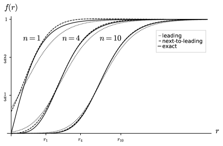
Figure 1: The numerical solution of the exact critical vortex equations for the scalar field $f(r)$ (solid lines), the leading asymptotic solution $e^{w(r-r_{n})}$ (dotted lines), and the next-to-leading approximation (dashed lines) for different winding numbers $n$.

The boundary layer. In this region the field dynamics is ultimately nonlinear. However, it crucially simplifies for large $n$. To see this we introduce a new radial coordinate $x=r-r_{n}$ so that in the boundary layer $x={\cal O}(1)$ and the expansion in $x/r_{n}$ converts into an expansion in $1/\sqrt{n}$. In the leading order in $x$ Eq. (3) reduces to a system of $n$-independent field equations with constant coefficients

$$\begin{split}&w^{\prime}+\gamma=0\,,\\ &\gamma^{\prime}-1+e^{2w}=0\,,\end{split}$$ (6)

where $w(x)=\ln f(r_{n}+x)$, $\gamma(x)={n}\left(a(r_{n}+x)-1\right)/r_{n}$, and prime stands for a derivative in $x$. The system can be resolved for $w$ which results in a second-order equation

$$\begin{split}&w^{\prime\prime}+1-e^{2w}=0\,.\end{split}$$ (7)

Figure 2: The values $f(r_{n})$ obtained from the numerical solution of the exact critical vortex equations (black dots), the asymptotic value $f(r_{n})=e^{w_{0}}$ (dotted line), and the next-to-leading approximation (solid line) as functions of the winding number $n$.

This equation has a first integral $I=w^{\prime 2}-e^{2w}+2w$ with $I=-1$ corresponding to the boundary condition $w(\infty)=0$. Thus Eq. (6) can be solved in quadratures with the result

$$\begin{split}&\int^{w(x)}_{w_{0}}{{\rm d}w\over(e^{2w}-2w-1)^{1/2}}=x\,,\\ &\gamma(x)=-(e^{2w(x)}-2w(x)-1)^{1/2}\,,\end{split}$$ (8)

where $w_{0}=w(0)$ is the second integration constant. It is determined by the boundary condition $w^{\prime}(x)\sim-x$ at $x\to-\infty$, which ensures that Eq. (8) can be matched to the core solution. This gives a new transcendental constant

$$w_{0}=-0.2997174398\ldots\,,$$ (9)

which determines a unique asymptotic solution in the boundary layer. It has the Taylor expansion $w(x)=\sum_{m=0}^{\infty}w_{m}x^{m}$ where $w_{1}=(e^{2w_{0}}-2w_{0}-1)^{1/2}$ and the higher order coefficients can be obtained recursively. The asymptotic behavior of the function at $x\to\infty$ reads

$$\begin{split}&w(x)\sim w_{\infty}e^{-\sqrt{2}x}\,,\\ &w(-x)\sim-{x^{2}\over 2}-{1\over 2}+\ldots\,,\end{split}$$ (10)

where $w_{\infty}=w_{0}\exp[\int_{w_{0}}^{0}(\sqrt{2}/(e^{2w}-2w-1)^{1/2}+{1/w}){\rm d}w]$. By using Eq. (10) it is straightforward to verify that up to corrections suppressed at large $n$ the boundary layer solution Eq. (8) coincides with the core solution Eq. (5) in the matching region $1\ll r_{n}-r\ll r_{n}$, where both approximations are valid. This is a rather nontrivial result since Eq. (5) does depend on $n$.

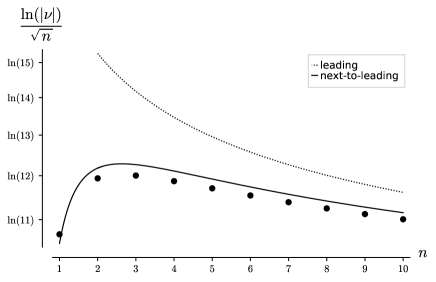
Figure 3: Scalar charge/magnetic dipole moment $\nu$ of a critical vortex obtained from the numerical solution of the exact vortex equations (black dots), the asymptotic result Eq. (12) (dotted line), and the next-to-leading approximation (solid line) as functions of the winding number $n$.

The vortex tail. For $(r-r_{n})/r_{n}={\cal O}(1)$ the boundary layer approximation breaks down and the coordinate dependence of the field equation coefficients should be restored. However, the deviation of the fields from the vacuum configuration is now exponentially small so the field equations linearize. The solution of the linearized theory is well known and reads

$$\begin{split}&f(r)\sim 1+{\nu\over 2\pi}K_{0}(\sqrt{2}r)+\ldots\,,\\ &a(r)\sim 1+{\mu\over 2\pi}{\sqrt{2}r}K_{1}(\sqrt{2}r)+\ldots\,,\end{split}$$ (11)

where $K_{m}(z)$ is the $m$th modified Bessel function. It describes the field of a point-like source of scalar charge $\nu$ and magnetic dipole moment $\mu$ with $\nu=\mu$ for critical coupling. Eqs. (8) and (11) should coincide in the second matching region $1\ll r-r_{n}\ll r_{n}$, which yields

$$\nu=4w_{\infty}\sqrt{\pi}e^{2\sqrt{n}+\ln(n)/4}\,.$$ (12)

Thus vortex scalar charge and magnetic dipole moment grow exponentially with the winding number.

Calculation of the higher order terms of the expansion in $1/\sqrt{n}$ is rather straightforward. Writing down the leading corrections to the asymptotic solutions $w$ and $\gamma$ as $\delta w/\sqrt{2n}$ and $\delta\gamma/\sqrt{2n}$, respectively, we get

$$\delta w(x)=Cw^{\prime}(x)+\int_{0}^{x}{w^{\prime}(x)\over w^{\prime 2}(z)}\int^{\infty}_{z}w^{\prime 2}(y){\rm d}y{\rm d}z\,,$$

$$\delta\gamma(x)=-{x}w^{\prime}(x)-\delta w^{\prime}(x)\,,$$ (13)

where $C=\int_{-\infty}^{0}[z/3+\int^{\infty}_{z}w^{\prime 2}(y)/w^{\prime 2}(z)dy]dz$.

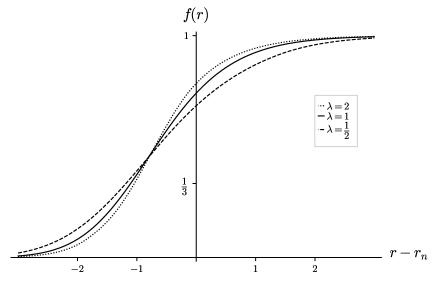
Figure 4: The asymptotic profiles of the scalar field $f(r)$ obtained by numerical solution of the effective vortex equations Eq. (16) for different values of scalar self-coupling as functions of $r-r_{n}$.

Let us now consider noncritical coupling $\lambda\neq 1$. In this case the order of the field equations cannot be reduced and they read

$$\begin{split}&{1\over r}{d\over dr}\left(r{df\over dr}\right)-\left[\lambda(f^{2}-1)+{n^{2}\over r^{2}}(1-a)^{2}\right]f=0\,,\\ &r{d\over dr}\left({1\over r}{da\over dr}\right)+{2}(1-a)f^{2}=0\,.\end{split}$$ (14)

Nevertheless, the general structure of the solution is quite similar to the critical case. Inside the core the contribution of the scalar potential to Eq. (14) is suppressed by $r^{2}/n^{2}$. Hence the core dynamics is not sensitive to $\lambda$ and the core solution is given by Eq. (5) up to the value of the integration constants which do depend on $\lambda$ through the matching to the nonlinear boundary layer solution. In particular the vortex size $r_{n}$ is determined by the region where the two terms in the square brackets of Eq. (14) become comparable and the core approximation breaks down, which gives the leading order result $r_{n}=\sqrt{2n}/\lambda^{1/4}$. Note that the approximately constant energy density in the core is now $\lambda\eta^{2}$ so that the total vortex energy in the large-$n$ limit is $T=2\pi\sqrt{\lambda}n\eta^{2}$. This agrees with the “wall-vortex” conjecture and numerical results for very large $n$ of Refs. Bolognesi:2005rj ; Bolognesi:2005zr . In the tail solution, Eq. (11), the argument of $K_{0}$ gets an additional factor of $\sqrt{\lambda}$ to account for the variation of the scalar field mass, while the scalar charge and the magnetic dipole moment are not equal anymore and have different leading behavior at $n\to\infty$

$$\begin{split}&|\nu|\sim e^{2\sqrt{n}\,\lambda^{1/4}+\ldots}\,,\qquad|\mu|\sim e^{2\sqrt{n}/\lambda^{1/4}+\ldots}\,.\end{split}$$ (15)

More accurately these parameters as well as the normalization of the scalar field in the core solution are determined by matching to the boundary layer solution. In the boundary layer by expanding in $x/r_{n}$ we get a system of $n$-independent equations with constant coefficients

$$\begin{split}&{f^{\prime\prime}}-\left[{\lambda}\left({f^{2}}-1\right)+{\gamma^{2}}\right]f=0\,,\\ &\gamma^{\prime\prime}-{2}\gamma{f^{2}}=0\,,\end{split}$$ (16)

with the boundary condition $\gamma(x)\sim\sqrt{\lambda}x$ at $x\to-\infty$. For $\lambda=1$ the proper solution is given by Eq. (8) and for any given $\lambda\neq 1$ it can be found numerically.

Finally we briefly discuss a simpler but quite interesting case of the vortices in Bose-Einstein condensate of a neutral scalar field. The corresponding vortex equation is obtained from the first line of Eq. (14) by setting $a=0$ and $\lambda=1$ (see, e.g. Landau ). Now the dynamics in the core of radius $r_{n}=n$ is described by a linear differential equation, while in the tail region $r_{n}+\delta\;\hbox to0.0pt{\lower 3.5pt\hbox{$\mathchar 0\relax\sim$}\hss}\raise 1.0pt\hbox{$<$}\;r$ with $\delta\propto n^{1/3}$ the derivative term is suppressed and the field equation becomes algebraic at $n\to\infty$. In contrast to the charged case the boundary layer does not form and the core and tail solutions can be polynomially matched over the interval $r_{n}\;\hbox to0.0pt{\lower 3.5pt\hbox{$\mathchar 0\relax\sim$}\hss}\raise 1.0pt\hbox{$<$}\;r\;\hbox to0.0pt{\lower 3.5pt\hbox{$\mathchar 0\relax\sim$}\hss}\raise 1.0pt\hbox{$<$}\;r_{n}+\delta$. This yields the asymptotic solution

$$f(r)=\left\{\begin{array}[]{l}C^{\prime}J_{n}(r)\,,\quad r\leq r_{n}\,,\\[3.0pt] \sqrt{\delta/2n}\left(1+{(r-r_{n})/\delta}\right),\,r_{n}<r<r_{n}+\delta\,,\\[3.0pt] \sqrt{1-{n^{2}/r^{2}}}\,,\quad r_{n}+\delta\leq r\,,\end{array}\right.$$ (17)

where $J_{n}(r)$ is the $n$th Bessel function, $C^{\prime}={3^{1/4}\pi^{1/2}\over 2^{1/2}}$, $\delta={2^{2/3}\pi n^{1/3}\over 3^{5/6}\Gamma^{2}(2/3)}$, and $\Gamma(z)$ is the Euler gamma-function. The vortex energy now is $T=\pi\eta^{2}n^{2}$, where a half of the contribution comes from the vortex tail. Curiously, for $\eta=1$ it is given by the area of a circle of radius $n$ while the critical vortex energy is equal to the corresponding circumference. The corrections to Eq. (17) are given by a series in $1/n^{1/3}$ and will be published elsewhere.

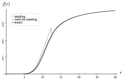
Figure 5: The numerical solution of the exact vortex equations for a neutral scalar field $f(r)$ (solid line), the leading asymptotic solution Eq. (17) (dotted line), and the next-to-leading approximation (dashed line) for $n=10$.

The results of numerical analysis of the large-$n$ approximation are presented in Figs. 1-5. In Fig. 1 the leading asymptotic result $e^{w(r-r_{n})}$ and the next-to-leading approximation which incorporates the ${\cal O}(1/\sqrt{n})$ terms are plotted against numerical solutions of the exact field equations for $f(r)$ with $\lambda=1$, $n=1,\,4,\,10$. In Figs. 2 and 3 the exact numerical values of $f(r_{n})$ and $\nu$, the natural characteristics of the vortex solution, are plotted against the asymptotic leading and next-to-leading results for $\lambda=1$, $n\leq 10$. The expansion reveals an impressive convergence and the next-to-leading approximation works reasonably well even for $n=1$. For completeness we present the result for the asymptotic profile of the boundary layer solution for the scalar field with $\lambda=1/2,\,1,\,2$ in Fig. 4. The numerical results for a neutral scalar field vortex with $n=10$ are given in Fig. 5

To summarize, we have elaborated a method of expansion in inverse powers of a topological quantum number. The method is quite general and can be applied to the study of topological solitons in a theory where the corresponding quantum number can be associated with a ratio of dynamical scales, e.g. to the multi-monopole solutions in Yang-Mills Higgs model, where only the case of vanishing scalar potential has been solved so far. When applied to axially symmetric vortices with large winding number $n$ the expansion is in powers of $1/n^{1/\alpha}$ with $\alpha=2$ for the charged and $\alpha=3$ for the neutral scalar field. In the large-$n$ limit the complex nonlinear vortex dynamics unravels. In particular, the field equations become integrable for critical coupling and reduce to an algebraic one for a neutral Bose-Einstein condensate. This yields simple asymptotic formulae for the shape and parameters capturing the main features of the giant vortices. The accuracy of the asymptotic result can be systematically improved and already after including the leading corrections the approximation works remarkably well all the way down to very low $n$.

- (1) A. A. Abrikosov, Sov. Phys. JETP 5, 1174 (1957) [Zh. Eksp. Teor. Fiz. 32, 1442 (1957)].
- (2) H. B. Nielsen and P. Olesen, Nucl. Phys. B 61, 45 (1973).
- (3) M. B. Hindmarsh and T. W. B. Kibble, Rept. Prog. Phys. 58, 477 (1995).
- (4) D. Tong, “TASI lectures on solitons: Instantons, monopoles, vortices and kinks,” [arXiv:hep-th/0509216].
- (5) P. L. Marston, W. M. Fairbank, Phys. Rev. Lett. 39, 1208 (1977).
- (6) P. Engels, I. Coddington, P. C. Haljan, V. Schweikhard, and E. A. Cornell, Phys. Rev. Lett. 90, 170405 (2003).
- (7) T. Cren, L. Serrier-Garcia, F. Debontridder, and D. Roditchev, Phys. Rev. Lett. 107, 097202 (2011).
- (8) E. B. Bogomolny, Sov. J. Nucl. Phys. 24, 449 (1976) [Yad. Fiz. 24, 861 (1976)].
- (9) H. J. de Vega and F. A. Schaposnik, Phys. Rev. D 14, 1100 (1976).
- (10) M. K. Prasad and C. M. Sommerfield, Phys. Rev. Lett. 35, 760 (1975).
- (11) E. Witten, Phys. Rev. Lett. 38, 121 (1977).
- (12) M. K. Prasad and P. Rossi, Phys. Rev. Lett. 46, 806 (1981).
- (13) S. Bolognesi, Nucl. Phys. B 730, 127 (2005).
- (14) S. Bolognesi and S. B. Gudnason, Nucl. Phys. B 741, 1 (2006).
- (15) E. M. Lifshitz, L. P. Pitaevskii, Statistical Physics, Part 2: Theory of the Condensed State, Vol. 9, 1st ed., Butterworth-Heinemann, Oxford, 1980.