An Increase in Small-planet Occurrence with Metallicity for Late-type Dwarf Stars in the Kepler Field and Its Implications for Planet Formation

Abstract

While it is well established that giant-planet occurrence rises rapidly with host star metallicity, it is not yet clear if small-planet occurrence around late-type dwarf stars depends on host star metallicity. Using the Kepler Data Release 25 planet candidate list and its completeness data products, we explore planet occurrence as a function of metallicity in the Kepler field’s late-type dwarf stellar population. We find that planet occurrence increases with metallicity for all planet radii $R_{\mathrm{p}}$ down to at least $R_{\mathrm{p}}\approx 2~{}R_{\oplus}$ and that in the range $2~{}R_{\oplus}\lesssim R_{\mathrm{p}}\lesssim 5~{}R_{\oplus}$ planet occurrence scales linearly with metallicity $Z$. Extrapolating our results, we predict that short-period planets with $R_{\mathrm{p}}\lesssim 2~{}R_{\oplus}$ should be rare around early M dwarf stars with $\mathrm{[M/H]}\lesssim-0.5$ or late M dwarf stars with $\mathrm{[M/H]}\lesssim+0.0$. This dependence of planet occurrence on metallicity observed in the Kepler field emphasizes the need to control for metallicity in estimates of planet occurrence for late-type dwarf stars like those targeted by Kepler’s K2 extension and the Transiting Exoplanet Survey Satellite (TESS). We confirm the theoretical expectation that the small planet occurrence–host star metallicity relation is stronger for low-mass stars than for solar-type stars. We establish that the expected solid mass in planets around late-type dwarfs in the Kepler field is comparable to the total amount of planet-making solids in their protoplanetary disks. We argue that this high efficiency of planet formation favors planetesimal accretion over pebble accretion as the origin of the small planets observed by Kepler around late-type dwarf stars.

1 Introduction

Planet formation is seeded by the metals present in a protoplanetary disk. It must be the case that the total heavy-element content of a protoplanetary disk provides an upper limit on the solid mass of planets formed in that disk. For that reason, there must be a metallicity below which even Earth-mass planets cannot form. Observations have shown that the occurrence of giant planets around FGKM dwarf stars rises rapidly with host star metallicity (e.g., Santos et al., 2004; Fischer & Valenti, 2005; Johnson & Apps, 2009a; Johnson et al., 2010). However, it is not clear how host star metallicity influences small planet occurrence.

Since both the metallicity and mass of a protoplanetary disk determine the amount of planet-making material available, we expect that the dependence of small-planet occurrence on metallicity should be stronger for low-mass stars than for solar-type stars. A star has accreted the vast majority of the total mass initially in its young disk prior to the epoch of planet formation, so any residual solids locked up in planets will not affect the observed metallicity of a star. Since the star and disk both formed from the same molecular core, the overall metallicities $Z_{\star}$ and $Z_{\mathrm{disk}}$ should be the same. The mass of a disk during the epoch of planet formation has been found to scale roughly linearly with stellar mass with fixed disk-to-star mass ratio $M_{\mathrm{disk}}/M_{\star}$ in the range $0.002\lesssim M_{\mathrm{disk}}/M_{\star}\lesssim 0.006$ (e.g., Andrews et al., 2013). Though there is more than an order-of-magnitude scatter in the Andrews et al. (2013) relation, those authors favor an inherently linear relationship between $M_{\mathrm{disk}}$ and $M_{\star}$. The net effect is that the amount of planet-making material available in a protoplanetary disk should scale roughly linearly with both stellar metallicity $Z_{\star}$ and mass $M_{\star}$.

Assuming the solar metallicity $Z_{\odot}=0.014$ (e.g., Asplund et al., 2009) and a disk-to-star mass ratio $M_{\mathrm{disk}}/M_{\star}=0.01$ (Andrews et al., 2013), an early M dwarf with $M_{\star}=0.6~{}M_{\odot}$ and $[\mathrm{M/H}]=-0.5$ would have less than $10~{}M_{\oplus}$ of planet-making material in its disk. In that case, the available planet-making material is much less than the amount required to make a single Neptune-size planet with radius $R_{\mathrm{p}}=4~{}R_{\oplus}$ (Neptune has at least $13~{}M_{\oplus}$ of metals as shown by Podolak et al., 2019). On the other hand, $10~{}M_{\oplus}$ of planet-making material would be enough to make an Earth-composition super-Earth mass planet with $R_{\mathrm{p}}\lesssim 1.8~{}R_{\oplus}$ (e.g., Zeng et al., 2019). If the timescale for growing Earth-mass embryos scales with the amount of planet-making material as suggested by detailed calculations (Movshovitz et al., 2010), then the probability of forming a planet with a significant gaseous envelope in the few Myr available before its parent protoplanetary disk is dissipated should also scale with the amount of planet-making material. There are hints that this effect becomes important at $[\mathrm{M/H}]\approx-0.5$ for solar-type stars (e.g., Petigura et al., 2018).

The expected relationship between small-planet occurrence and metallicity for low-mass stars has been hard to confirm because metallicity measurements for low-mass stars are inherently difficult. Stellar metallicity has traditionally been measured using metal lines in optical or near-infrared spectra (e.g., Rojas-Ayala et al., 2010, 2012; Mann et al., 2013a, b; Muirhead et al., 2014; Neves et al., 2014; Newton et al., 2014). Metal lines and molecular absorption bands are so common in the optical spectra of cool dwarf stars that it often becomes impossible to set the continuum level necessary for the measurement of equivalent widths. The lack of laboratory data necessary to handle molecular features has been an issue as well.

Broadband photometry also carries metallicity information, albeit at a less precise level for individual stars. Applied to large samples of stars in the same place on the sky distributed over a similar range in distance, photometric metallicities become precise indicators of relative metallicity. Bonfils et al. (2005) and Johnson & Apps (2009b) were among the first to compare the photometric metallicities of late-type dwarf stars observed to host or lack planets discovered with the Doppler technique with the goal to explore the connection between planet occurrence and metallicity. Schlaufman & Laughlin (2010) built on these groundbreaking studies and found a hint that M dwarfs hosting Neptune-mass planets are more metal-rich than similar stars without planets. Leveraging the large number of small planets discovered early in the Kepler mission, Schlaufman & Laughlin (2011) found that the average $g-r$ of late-type dwarf stars with small-planet candidates was $4\sigma$ redder than the average color of a control sample of similar stars without identified planet candidates. They argued that their observation was evidence for a metallicity difference between late-type dwarf stars with and without small planets.

The Schlaufman & Laughlin (2011) result was criticized by Mann et al. (2012, 2013b), who argued that the $g-r$ photometric metallicity indicator used by Schlaufman & Laughlin (2011) is insensitive to metallicity and that the possible presence of giant stars mistaken for dwarf stars in the Schlaufman & Laughlin (2011) control sample could produce a similar $g-r$ offset unrelated to metallicity. Both of these criticisms can now be conclusively addressed. Photometric metallicity relations for late-type dwarf stars calibrated by reliable APO Galactic Evolution Experiment (APOGEE) high-resolution $H$-band spectroscopy are now available (Majewski et al., 2016; Schmidt et al., 2016). Kepler asteroseismology (Hekker et al., 2011; Huber et al., 2011; Stello et al., 2013; Huber et al., 2014; Mathur et al., 2016; Yu et al., 2016, 2018) and Gaia DR2 parallaxes (Gaia Collaboration et al., 2016, 2018; Arenou et al., 2018; Hambly et al., 2018; Lindegren et al., 2018; Luri et al., 2018) enable the construction of samples of dwarf stars without planet candidates completely free of subgiant or giant star contamination. Advances in the analysis of Kepler data and the public availability of its completeness data products now permit differential planet occurrence calculations. Thanks to these developments, photometric metallicities have become a powerful tool for the exploration of the small-planet occurrence–metallicity relation.

Advances in the theory of planet formation have also revealed the possible significance of the accretion of “pebbles”, or material significantly smaller than the km-size planetesimals historically studied (Ormel & Klahr, 2010; Lambrechts & Johansen, 2012). This “pebble accretion” process invokes the accretion by planetary embryos of small particles experiencing strong aerodynamic drag. Since not all of this rapidly migrating material can be accreted by a planetary embryo, pebble accretion is inherently lossy in the sense that more than 90% of a disk’s initial complement of planet-making material falls onto its host star (e.g., Lin et al., 2018). On the other hand, the classical “planetesimal accretion” process is thought to be much more efficient in the sense that a larger fraction of a disk’s initial complement of planet-making material is locked up in planetesimals. Efficient planet formation seems to have occurred in the solar system, as the amount of planet-making material in the minimum-mass solar nebula (MMSN - Weidenschilling, 1977; Hayashi, 1981) is within a factor of two of that expected in a disk with $M_{\mathrm{disk}}\sim 0.01~{}M_{\odot}$ and $Z_{\mathrm{disk}}\sim Z_{\odot}=0.014$. We therefore propose that the efficiency of planet formation—the fraction of a protoplanetary disk’s initial complement of planet-making material sequestered in planets—is diagnostic of the relative importance of pebble/planetesimal accretion in the planet formation process.

As we will show, it is now possible to use photometric metallicities to explore small-planet occurrence around late-type dwarf stars as a function of metallicity using Kepler data. In this paper, we calculate planet occurrence as a function of metallicity, orbital period, and planet radius in the population of late-type dwarf stars observed by Kepler during its prime mission. Using the Kepler Data Release (DR) 25 Kepler Object of Interest (KOI) planet candidate list (Thompson et al., 2018), we find that that planet occurrence increases with metallicity for all planet radii down to at least $R_{\mathrm{p}}\approx 2~{}R_{\oplus}$ and that in the range $2~{}R_{\oplus}\lesssim R_{\mathrm{p}}\lesssim 5~{}R_{\oplus}$ planet occurrence scales linearly with metallicity. In Section 2 we discuss our sample selection, describe the photometric effective temperature and metallicity relations we use, and outline the process we use to remove giant stars from our sample of stars without planet candidates. We split both planet candidate-host and non-planet-candidate-host samples into metal-rich and metal-poor subsamples and illustrate two different occurrence calculations in Section 3. We then calculate planet formation efficiency in an attempt to infer the relative importance of planetesimal accretion and pebble accretion. In Section 4 we discuss our results and their implications for the theory of planet formation. We conclude and summarize our findings in Section 5.

2 Data

We seek to assemble the sample of late-type dwarf stars with Kepler light curves that have been searched for transiting planet candidates. To do so, we select late-type stars from the Kepler Input Catalog (KIC - Brown et al., 2011) with effective temperature $T_{\mathrm{eff}}$ in the range 3600 K $\lesssim T_{\mathrm{eff}}\lesssim$ 4200 K using the following empirical relations from Schmidt et al. (2016) based on spectroscopic stellar parameters derived from APOGEE high-resolution $H$-band spectroscopy

$$[\mathrm{M/H}] = a_{0}+a_{1}\left(r-z\right)+a_{2}\left(W1-W2\right),$$ (1)

$$T_{\mathrm{eff}} = b_{0}+b_{1}\left(r-z\right)+b_{2}\mathrm{[M/H]},$$ (2)

with the coefficients $a_{i}=(-0.822,0.634,-4.508)$ and $b_{i}=(4603.4,-576.5,225.0)$. Schmidt et al. (2016) considered all color combinations possible with Sloan Digital Sky Survey (SDSS) $ugriz$, Two Micron All Sky Survey (2MASS - Skrutskie et al., 2006) $JHK_{\mathrm{s}}$, and Wide-field Infrared Survey Explorer (WISE - Wright et al., 2010; Mainzer et al., 2011) $W1$ and $W2$ photometry. They found that a linear relation using $r-z$ and $W1-W2$ was best able to reproduce the spectroscopic stellar parameters $T_{\mathrm{eff}}$ and $\mathrm{[M/H]}$. The uncertainties in individual $\mathrm{[M/H]}$ and $T_{\mathrm{eff}}$ estimates produced using Equations (1) and (2) are approximately 0.2 dex in $[\mathrm{M/H}]$ and 100 K in $T_{\mathrm{eff}}$. We require all late-type stars in our sample to have been observed for at least one quarter during the Kepler mission.

It is well known that the surface gravity $\log{g}$ estimates in the KIC are imperfect (e.g., Mann et al., 2012; Dressing & Charbonneau, 2015). To ensure that there are no giant stars in our sample, we reject stars identified as giants via either asteroseismic oscillations or Gaia DR2 parallaxes. We first select Kepler target stars with KIC $\log{g}>4$. We then remove stars identified through asteroseismology as subgiants or as giants/red clump stars by Hekker et al. (2011), Huber et al. (2011), Stello et al. (2013), Huber et al. (2014), Mathur et al. (2016), or Yu et al. (2016, 2018). We also use Gaia DR2 parallaxes to calculate Gaia $G$-band absolute magnitudes and then exclude 11 giant stars that are several magnitudes above the Hamer & Schlaufman (2019) empirical Pleiades zero-age main sequence.

We cross match this purified sample of late-type dwarf stars with the Kepler DR25 list of KOIs dispositioned as planet candidates (Thompson et al., 2018). We use the homogeneous DR25 planet candidate list because it was generated in a fully automated fashion that eliminated human vetting of threshold crossing events. That lack of intervention made its completeness straightforward to algorithmically assess. Because giant planet host stars are known to be metal rich, we exclude from our analysis stars that host planets with $R_{\mathrm{p}}>5~{}R_{\oplus}$. We also verified that using the updated stellar radii from Berger et al. (2018) did not change any of our subsequent conclusions.

Our final planet candidate-host sample consists of the 99 late-type dwarfs with at least one planet candidate with $R_{\mathrm{p}}\leq 5~{}R_{\oplus}$ listed in Table 1. We refer to these stars as our planet candidate-host sample from this point on. We also select a sample of 3,395 late-type dwarfs that were part of the main transiting exoplanet search program, passed all of our selection criteria listed above, and have no detected planet candidate. We list these stars in Table 2 and refer to them as our non-planet-candidate-host sample from here. We plot $r-z$ versus $W1-W2$ color–color plots for both our planet candidate-host and non-planet-candidate-host samples in Figure 1. We plot photometric $T_{\mathrm{eff}}$ and $[\mathrm{M/H}]$ values inferred using Equations (1) and (2) for both our planet candidate-host and non-planet-candidate-host samples in Figure 2.

Table 1: Late-type Dwarf Kepler Targets with at Least One DR25 Planet Candidate with $R_{\mathrm{p}}\leq 5~{}R_{\oplus}$

KIC Number	Kepler Name	KOI Name	R.A.	Decl.	$r$	$z$	$W1$	$\sigma_{W1}$	$W2$	$\sigma_{W2}$
			(deg)	(deg)	(mag)	(mag)	(mag)	(mag)	(mag)	(mag)
10118816	$\cdots$	K01085	281.05011	47.188148	15.29	14.28	12.164	0.023	12.103	0.021
6921944	Kepler-1105	K02114	281.11176	42.454910	15.14	14.31	12.164	0.023	12.193	0.022
7582691	$\cdots$	K04419	281.11646	43.282440	15.16	14.29	12.145	0.023	12.132	0.022
6497146	Kepler-438	K03284	281.64581	41.951092	14.61	13.39	11.080	0.023	11.075	0.020
7870390	Kepler-83	K00898	282.23251	43.665630	15.76	14.96	12.880	0.023	12.891	0.024
8346392	Kepler-777	K01141	282.72406	44.346470	15.97	15.04	13.030	0.023	13.055	0.024
7094486	Kepler-1009	K01907	282.85992	42.665760	15.34	14.40	12.257	0.023	12.268	0.022
10386984	Kepler-658	K00739	282.98380	47.578590	15.52	14.63	12.535	0.023	12.571	0.022
7871954	Kepler-303	K01515	283.13547	43.657051	14.40	13.58	11.550	0.023	11.550	0.021
10122538	Kepler-1388	K02926	283.33606	47.174541	16.30	15.39	13.269	0.023	13.313	0.025

Note. — The typical $r$- and $z$-band uncertainties are 0.02 mag (Brown et al., 2011). This table is ordered by right ascension and is available in its entirety in the machine-readable format.

Table 2: Late-type Dwarf Kepler Targets with No Observed Planet Candidates

KIC Number	R.A.	Decl.	$r$	$z$	$W1$	$\sigma_{W1}$	$W2$	$\sigma_{W2}$
	(deg)	(deg)	(mag)	(mag)	(mag)	(mag)	(mag)	(mag)
7797376	279.708780	43.53535	15.78	15.14	13.108	0.024	13.106	0.025
7867105	279.996150	43.67716	14.32	13.53	11.488	0.023	11.520	0.021
7867279	280.120470	43.68729	15.39	14.70	12.614	0.023	12.642	0.023
7658133	280.122220	43.35148	15.52	14.80	12.790	0.022	12.796	0.023
10382584	280.132140	47.59633	15.85	14.93	12.756	0.023	12.793	0.024
7581219	280.137160	43.21006	15.97	14.68	12.352	0.023	12.331	0.021
10317398	280.232649	47.45096	15.03	14.39	12.458	0.023	12.436	0.022
10251684	280.305889	47.39492	15.09	14.36	12.340	0.022	12.354	0.022
7581487	280.315260	43.22374	15.76	14.62	12.377	0.023	12.357	0.022
7867585	280.358460	43.61532	16.01	15.01	12.824	0.023	12.821	0.023

Note. — The typical $r$- and $z$-band uncertainties are 0.02 mag (Brown et al., 2011). This table is ordered by right ascension and is published in its entirety in the machine-readable format.

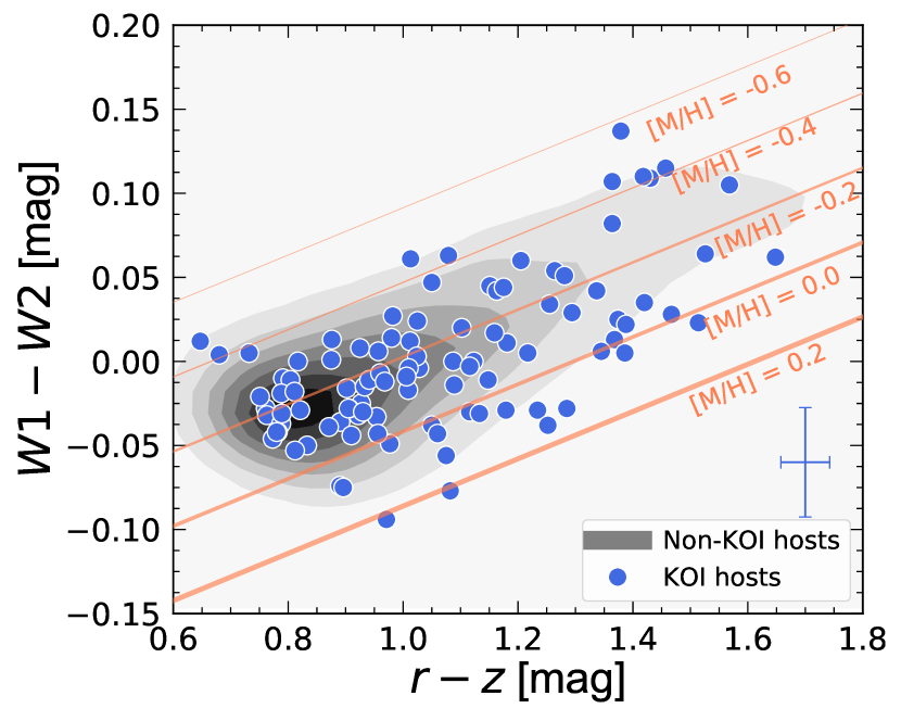
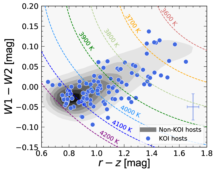
Figure 1: Distribution of late-type dwarf stars in the $r-z$ versus $W1-W2$ color–color plot. The blue circles represent the planet candidate-host sample while the gray shading represents the distribution of the non-planet-candidate-host sample after kernel smoothing. We represent the typical color uncertainties with the crosses at the bottom right of each plot. Left: solid orange lines represent lines of constant $[\mathrm{M/H}]$ according to Schmidt et al. (2016). Right: dashed curves represent lines of constant $T_{\mathrm{eff}}$ according to Schmidt et al. (2016).

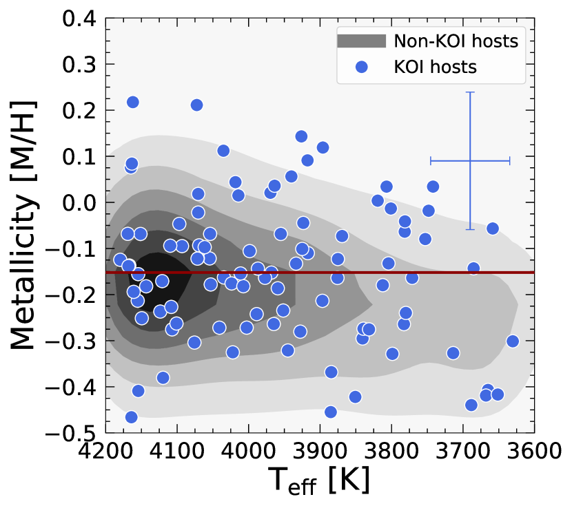
Figure 2: $\mathrm{[M/H]}$ as a function of $T_{\mathrm{eff}}$ for planet candidate-host and non-planet-candidate-host samples inferred using $r-z$ and $\mathrm{W1}-\mathrm{W2}$ colors in Equations (1) and (2). The blue circles represent the planet candidate-host sample while the gray shading represents the distribution of the non-planet-candidate-host sample after kernel smoothing. The red line at $[\mathrm{M/H}]=-0.15$ indicates the median host star metallicity for the planet candidate sample. While there are fewer stars above the red line than below it, the metal-rich stars host more multiple planet candidate systems. We represent the typical $[\mathrm{M/H}]$ and $T_{\mathrm{eff}}$ uncertainties resulting from uncertainties in the input photometry with the cross at the top right.

3 Analysis

We explore the connection between host star metallicity and small-planet occurrence in three ways. First, we use logistic regression to estimate the significance of metallicity and effective temperature for the prediction of planet occurrence in our complete sample. We next separate our complete sample into metal-rich and metal-poor subsamples for which we independently calculate planet occurrence as a function of metallicity, orbital period $P$, and planet radius $R_{\mathrm{p}}$ using the Kepler DR25 completeness data products. We then use a mass–radius relation combined with the small-planet occurrence maps inferred for our complete sample as well as our metal-rich and metal-poor subsamples to roughly estimate the planet formation efficiency in the protoplanetary disks that once existed around the stars in our sample.

3.1 Logistic Regression

We use logistic regression—a natural extension of linear regression for probability—to obtain a first look at the relationship between host star metallicity & effective temperature and the probability of the presence of a small planet candidate in the system $P_{\mathrm{host}}$. We use the logistic regression model

$$P_{\mathrm{host}} = \frac{1}{1+e^{-x}},$$ (3)

$$x = \beta_{0}+\beta_{1}T_{\mathrm{eff}}+\beta_{2}[\mathrm{M/H}],$$ (4)

and the statsmodel.logit (Genz, 2004; Seabold & Perktold, 2010) implementation of logistic regression. We give the result of our calculation in Table 3.

Table 3: Logistic Regression Results

Variable	Value	Uncertainty	$t$-statistic	$p$-value
$T_{\mathrm{eff}}$	$-7.6\times 10^{-4}$	$5.9\times 10^{-4}$	$-1.3$	$0.20$
$[\mathrm{M/H}]$	$1.8$	$0.65$	$2.8$	$0.010$

We find that the coefficient for metallicity in the logistic regression equation is positive and significantly different than zero, while the coefficient for effective temperature is consistent with zero (see Table 3). The implication is that planet occurrence increases with host star metallicity and is insensitive to host star effective temperature. The coefficient of a continuous predictor variable in a logistic regression model gives the expected change in the natural logarithm of the odds ratio of the modeled outcome with a one-unit change in that continuous predictor variable. Since we will subsequently find in the next subsection that the metallicity difference between our metal-rich and metal-poor subsamples is about 0.3 dex, we use our logistic regression model to estimate the effect of a 0.3 dex change in $[\mathrm{M/H}]$ on the probability of finding a planet candidate in a system $P_{\mathrm{host}}$. When the probability of an event is small and therefore $x$ must be small as well, the logistic regression function is approximately an exponential regression $P=e^{x}$ and the coefficients $\beta_{i}$ can be interpreted as the fractional change of the odds of an event’s occurrence. We find that $P_{\mathrm{host}}([\mathrm{M/H}]+0.3)=1.69_{-0.30}^{+0.36}~{}P_{\mathrm{host}}([\mathrm{M/H}])$. In words, the probability that a late-type dwarf star was observed by Kepler to host at least one small planet candidate increases by a factor of about $1.69_{-0.30}^{+0.36}$ for a 0.3 dex change in $[\mathrm{M/H}]$ (a factor of two in $Z_{\star}$).

The logistic regression analysis handles single- and multiple-planet systems in the same way and therefore does not account for multiplicity. It does not control for the decrease in transit probability with semimajor axis or the incompleteness of the Kepler DR25 planet candidate list. It implicitly assumes that a star with no observed planet candidates is equivalent to a star without planets. This last assumption is only valid in the parts of parameter space where planet occurrence is low (i.e., $P\lesssim 10$ days and $2~{}R_{\oplus}\lesssim R_{\mathrm{p}}\lesssim 5~{}R_{\oplus}$). Because planet occurrence increases with both increasing orbital period and with decreasing planet radius, it is important to account for transit probability and Kepler DR25 completeness to explore the connection between host star metallicity and small-planet occurrence for the much more common long-period and/or small-radius planets.

3.2 Occurrence as a Function of Metallicity, Orbital Period, and Planet Radius

To complement the logistic regression analysis in the previous subsection, we calculate planet occurrence as a function of metallicity, orbital period, and planet radius using the Kepler DR25 planet candidate list and its completeness data products. This approach takes into account planet multiplicity and allows us to explore the connection between host star metallicity and small-planet occurrence at longer periods and smaller radii than the logistic regression approach.

We first separate our complete sample into metal-rich and metal-poor subsamples by splitting at the metallicity that separates our planet candidate-host sample into two nearly equal halves. We split our complete sample into two nearly equally sized subsamples to minimize the effects of sample size differences. We therefore set the dividing line at $[\mathrm{M/H}]=-0.15$ as shown Figure 2. The resulting metal-rich subsample has 74 planet candidates (49 planet candidate hosts) and 1,299 non-planet-candidate hosts while the metal-poor subsample has 76 planet candidates (50 planet-candidate hosts) and 2,096 non-planet-candidate hosts. We find that the average metallicities of our metal-rich and metal-poor samples are $[\mathrm{M/H}]=+0.0$ and $[\mathrm{M/H}]=-0.3$ respectively. Because one star might host multiple planet candidates, it is impossible to exactly divide the planet candidate hosts such that the number of planet candidates in the two subsamples are exactly equal. If instead we split our complete sample into two subsamples each with an equal number of stars, then the median metallicity of the metal-rich subsample would decrease by 0.01 dex in [M/H] and the median metallicity of the metal-rich subsample would remain the same.

To go from the observed frequency of planet candidates to their underlying occurrence, it is necessary to divide the observed frequency by its completeness. For each star in both subsamples, we use the KeplerPORTS software described in Burke & Catanzarite (2017) to estimate the completeness of the Kepler Pipeline that produced the DR25 planet candidate list as a function of orbital period and planet radius. We present in Figure 3 an example completeness map for KIC 1577265 (a randomly selected star from our complete sample).

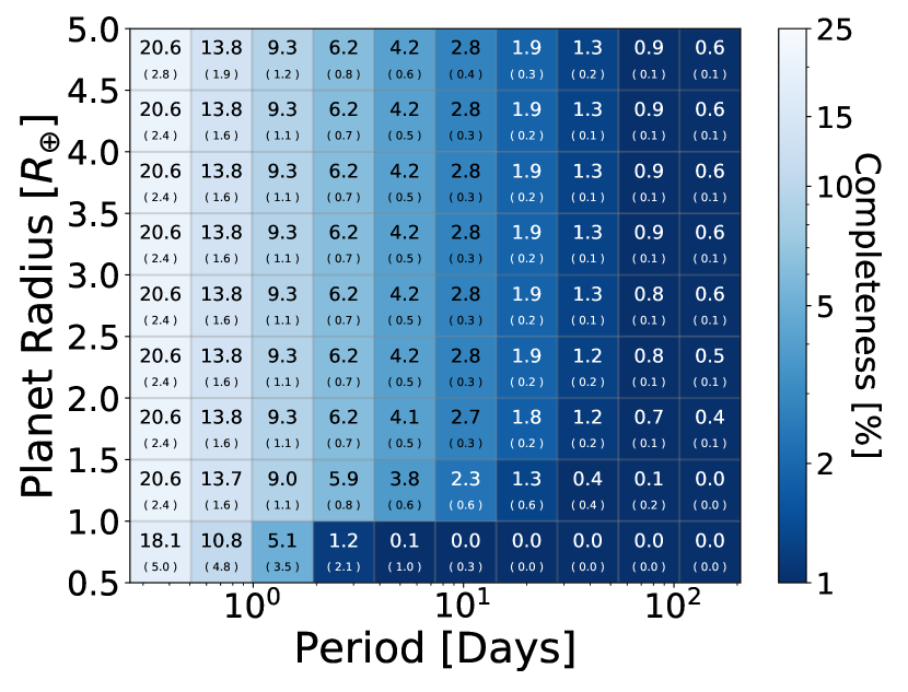
Figure 3: Example completeness map for KIC 1577265. The values in every cell denote the completeness and the scatter of completeness within the cell in percent.

We combine individual completeness maps for all stars in each subsample to obtain representative completeness maps for both the metal-rich and metal-poor subsamples. For each point in orbital period–planet radius space, we take the average value of the completeness maps produced for all stars in a given subsample. We thereby obtain a representative completeness map that corresponds to the typical completeness averaged over an entire subsample. Completeness maps that have smaller planet radius cells than the typical planet candidate’s radius uncertainty are oversampled. Since planet candidates only sparsely populate orbital period–planet radius space and because planet candidate radius uncertainties are non-negligible, we then resample the representative completeness maps at lower resolution. We evenly divide orbital period–planet radius space in $\log_{10}{P}$ and $R_{\mathrm{p}}$. For each cell, we take the representative completeness value to be the median of all completeness estimates in that cell. For example, in Figure 3 the value in each cell is the median of all individual completeness estimates in that cell from the initial higher-resolution completeness map.

We compute the occurrence of planet candidates as a function of orbital period and planet radius in both metal-rich and metal-poor subsamples using their the representative completeness maps. The occurrence in each cell depends on the total number of observed planet candidates $N_{\mathrm{PC}}$ and the total number of equivalent stars searched $N_{\mathrm{\star}}$ in that cell. We define $N_{\star}$ as the product of our estimated representative completeness in that cell and the total number of stars in a subsample. Since there are uncertainties in the measurement of each planet candidate’s orbital period and radius, we use a 1,000 iteration Monte Carlo simulation to distribute the impact of an individual planet candidate detection across multiple cells using a two-dimensional Gaussian kernel with a diagonal covariance matrix with the 1-$\sigma$ period and radius uncertainties on the diagonal. We then define $N_{\mathrm{PC}}$ as the number of counts in each cell averaged over the Monte Carlo simulation.

We adopt a Bayesian framework to estimate planet occurrence $\eta$. We model occurrence with a binomial likelihood and use a Beta distribution prior $\mathrm{Beta}\left(\alpha,\beta\right)$. In that situation, the Beta distribution is a conjugate prior and the posterior distribution of occurrence will be a Beta distribution that depends on the prior parameters, $N_{\mathrm{PC}}$, and $N_{\star}$

$$P\left(\eta|N_{\mathrm{PC}},N_{\star}\right) =$$

$$\mathrm{Beta}\left(\alpha+N_{\mathrm{PC}},\beta+N_{\star}-N_{\mathrm{PC}}\right),$$

where $\alpha$ and $\beta$ are parameters of the prior. We assume a weak uninformative prior with $\alpha=\beta=1$.

We plot the results of our occurrence calculations in Figures 4 and 5 and give them in tabular form in Table 4. Figure 4 shows planet candidate occurrence as a function of orbital period and planet radius for both our metal-rich and metal-poor subsamples, while Figure 5 shows planet candidate occurrence as a function of orbital period and planet radius for our complete sample. The differences in planet occurrence between the metal-rich and metal-poor subsamples illustrate the effect of metallicity on small planet formation: small planets are less common around metal-poor stars than around metal-rich stars. We indicate cells with no detected planet candidates in Table 4 and with black borders in both Figures 4 and 5. Our metal-rich and metal-poor subsamples are large enough and Kepler DR25’s completeness is high enough that for cells with $P\lesssim 100$ days and $R_{\mathrm{p}}\gtrsim 1~{}R_{\oplus}$ the product of sample size and completeness is larger than 10 (see Table 4). In this case, the signal implicit in a non-detection is at least an a factor of five larger than the signal weakly implied by our prior.

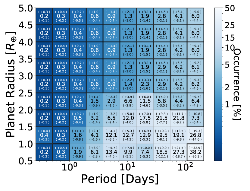
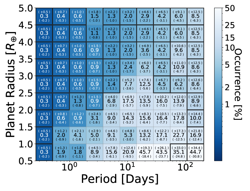
Figure 4: Planet candidate occurrence in metallicity–period–planet radius space with an uninformative prior. The values in each cell are the occurrence of planet candidates in that cell and its uncertainty. All values are expressed as percents. Cells with heavy borders have no detected planet candidates. Left: small planet candidate occurrence in our metal-poor subsample. Right: small planet candidate occurrence in our metal-rich subsample. Planet candidates are significantly more common in the metal-rich subsample than in the metal-poor subsample. The product of our samples’ sizes and Kepler DR25’s completeness indicate that the amount of information implicit in a non-detection is at least a factor of five larger than the signal weakly implied by our prior for cells with $P\lesssim 100$ days and $R_{\mathrm{p}}\gtrsim 1~{}R_{\oplus}$.

Figure 5: Planet candidate occurrence as a function of period and planet radius in our complete sample. The values in each cell are the occurrence of planet candidates in that cell and its uncertainty. All values are expressed as percents. Cells with heavy borders have no detected planet candidates. The product of our samples’ sizes and Kepler DR25’s completeness indicate that the amount of information implicit in a non-detection is at least an order-of-magnitude larger than the signal weakly implied by our prior for cells with $P\lesssim 100$ days and $R_{\mathrm{p}}\gtrsim 1~{}R_{\oplus}$.

Table 4: Occurrence of Small Planet Candidates in the Kepler Field with Late-type Dwarf Primaries as a Function of Metallicity

Planet Radius	Period	Occurrence	$\mathrm{[M/H]~{}Description}$	PC Detection Flag	Completeness	Equivalent Number
						of Stars Searched
($R_{\oplus}$)	(days)	(%)			(%)
0.5-1.0	0.3-0.5	${0.2}^{+0.3}_{-0.2}$	MP	0	16.41	226
0.5-1.0	0.5-1.0	${0.3}^{+0.5}_{-0.2}$	MP	0	10.22	141
0.5-1.0	1.0-1.9	${1.9}^{+1.4}_{-0.9}$	MP	1	6.21	85
0.5-1.0	1.9-3.8	${6.1}^{+3.0}_{-2.3}$	MP	1	3.64	50
0.5-1.0	3.8-7.3	${13.4}^{+5.7}_{-4.6}$	MP	1	1.97	27
0.5-1.0	7.3-14.3	${9.9}^{+7.4}_{-5.1}$	MP	1	0.99	14
0.5-1.0	14.3-27.9	${7.4}^{+10.0}_{-5.3}$	MP	1	0.46	6
0.5-1.0	27.9-54.5	${18.5}^{+19.0}_{-12.1}$	MP	1	0.20	3
0.5-1.0	54.5-106.2	${27.3}^{+27.5}_{-18.7}$	MP	1	0.08	1
0.5-1.0	106.2-207.2	${38.2}^{+32.9}_{-26.3}$	MP	0	0.03	0

Note. — In the column “[M/H] Description” the strings “MP”, “MR”, and “All”, correspond to our metal-poor, metal-rich, and complete samples. This table is published in its entirety in the machine-readable format.

Planets with $R_{\mathrm{p}}\gtrsim 2~{}R_{\oplus}$ are almost certain to possess significant H/He envelopes (e.g., Rogers, 2015; Chen & Kipping, 2017). We therefore separately study the difference in “rocky” ($0.5~{}R_{\oplus}\lesssim R_{\mathrm{p}}\lesssim 2~{}R_{\oplus}$) and “H/He envelope” ($2~{}R_{\oplus}\lesssim R_{\mathrm{p}}\lesssim 5~{}R_{\oplus}$) planet occurrence between our metal-rich and metal-poor subsamples. This $R_{\mathrm{p}}\approx 2~{}R_{\oplus}$ boundary also corresponds to the so-called “Fulton Gap” (e.g., Fulton et al., 2017; Fulton & Petigura, 2018; Berger et al., 2018). To faithfully account for the effect of uncertainty on this calculation, we conduct a Monte Carlo simulation. For every cell of each of the metal-rich and metal-poor subsamples, we sample planet candidate occurrence from its posterior distribution. For each cell, we then take the planet candidate occurrence difference between the metal-rich and metal-poor subsamples and sum the difference across all periods (excluding the longest-period cells because of their sub-percent completeness levels). We obtain a number that describes the cumulative differential occurrence between metal-rich and metal-poor subsamples. We repeat this process 10,000 times to fully sample the differential occurrence distribution. We take the median and the 16th and 84th percentiles of the distribution as the typical planet candidate occurrence difference and its associated uncertainty. We call this statistic our “planet occurrence difference” from here. We visualize these results in Figure 6 and present them in tabular form in Table 5.

We calculate the enhanced occurrence of planets in the metal-rich subsample relative to the occurrence of planets in the metal-poor sample in one more way. For every cell of each of the metal-rich and metal-poor subsamples, we sample planet candidate occurrence from its posterior distribution and sum over all cells in a subsample. We divide the summed occurrence calculated for the metal-rich subsample by the summed occurrence calculated for the metal-poor subsample to calculate a statistic we define as the occurrence “factor of enhancement”. We repeat this process 10,000 times to fully sample the factor of enhancement distribution. We report the median and the $16$th and $84$th percentiles of the factor of enhancement distribution in Table 5 and present it visually in Figure 6.

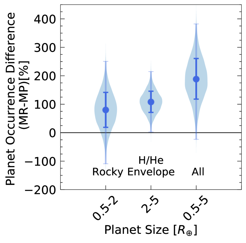
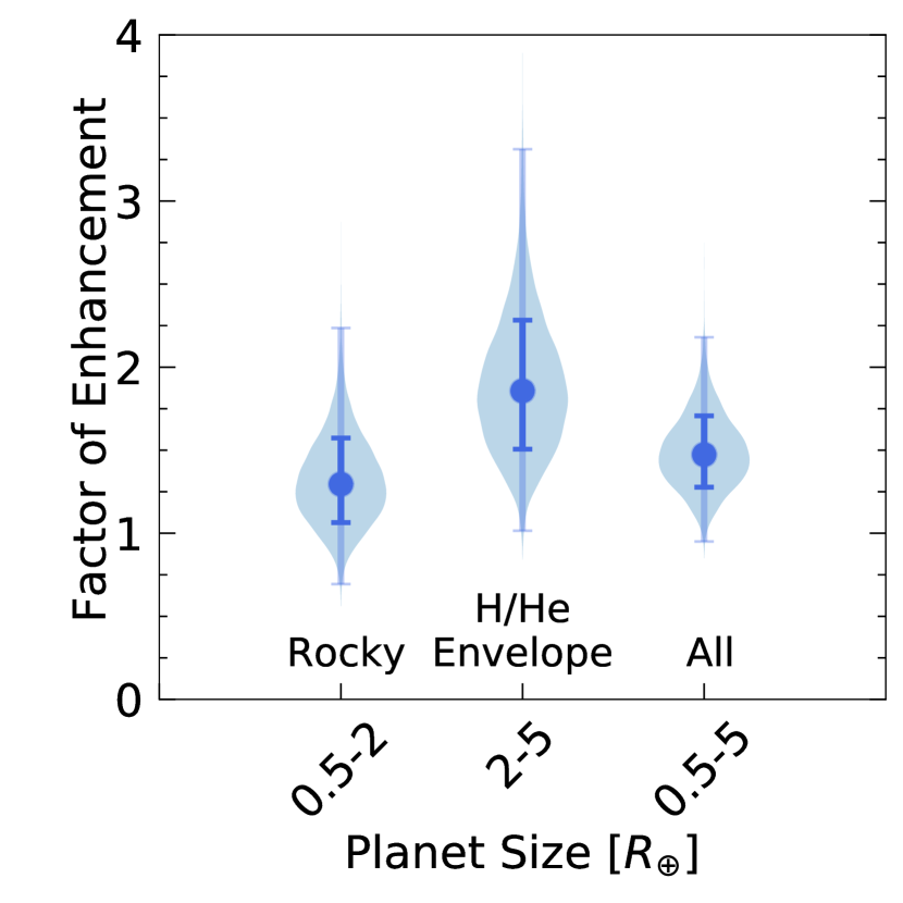
Figure 6: Violin plots with differences in planet candidate occurrence between metal-rich and metal-poor subsamples as a function of planet radius. The dark blue bars denote the 16th and 84th percentiles (i.e., the 1-$\sigma$ region) while the light blue bars represents the 0.13th and 99.7th percentiles (i.e., the 3-$\sigma$ region). Left: planet occurrence difference as a function of planet radius. Right: factor of enhancement as a function of planet radius. The occurrence of planet candidates is significantly higher in our metal-rich subsample both for the entire range of radii we study $0.5~{}R_{\oplus}\lesssim R_{\mathrm{p}}\lesssim 5~{}R_{\oplus}$ and for H/He envelope planets with $2~{}R_{\oplus}\lesssim R_{\mathrm{p}}\lesssim 5~{}R_{\oplus}$. Our results are inconclusive for rocky planets with $0.5~{}R_{\oplus}\lesssim R_{\mathrm{p}}\lesssim 2~{}R_{\oplus}$.

Table 5: Relative Planet Candidate Occurrence Statistics Observed Between the Metal-rich and Metal-poor Subsamples

Category	Occurrence Difference	Factor of Enhancement
	(%)
Rocky ($0.5~{}R_{\oplus}\lesssim R_{\mathrm{p}}\lesssim 2~{}R_{\oplus}$)	$80^{+62}_{-62}$	$1.3^{+0.3}_{-0.2}$
H/He Envelope ($2~{}R_{\oplus}\lesssim R_{\mathrm{p}}\lesssim 5~{}R_{\oplus}$)	$108^{+38}_{-37}$	$1.9^{+0.4}_{-0.4}$
All ($0.5~{}R_{\oplus}\lesssim R_{\mathrm{p}}\lesssim 5~{}R_{\oplus}$)	$188^{+72}_{-70}$	$1.5^{+0.3}_{-0.2}$

For planet candidates over the complete range in planet radius we study $0.5~{}R_{\oplus}\lesssim R_{\mathrm{p}}\lesssim 5~{}R_{\oplus}$, the occurrence of planet candidates in the metal-rich subsample is a factor of $1.5^{+0.3}_{-0.2}$ higher than in the metal-poor subsample. For H/He envelope planet candidates ($2~{}R_{\oplus}\lesssim R_{\mathrm{p}}\lesssim 5~{}R_{\oplus}$), the occurrence of planet candidates in the metal-rich subsample is a factor of $1.9\pm 0.4$ higher than in the metal-poor subsample. We note that the difference in $[\mathrm{M/H}]$ between our metal-rich and metal-poor subsamples is about 0.3 dex or a factor of two in $Z_{\star}$, so the occurrence of planets with $R_{\mathrm{p}}\gtrsim 2~{}R_{\oplus}$ grows roughly linearly with $Z_{\star}$ in our sample. We also note that none of the planet candidates with $3~{}R_{\oplus}\lesssim R_{\mathrm{p}}\lesssim 5~{}R_{\oplus}$ in our complete sample were found in the metal-poor subsample. We therefore conclude that for late-type dwarf stars metallicity is an important parameter in planet occurrence calculations that should not be neglected for planets with $R_{\mathrm{p}}\gtrsim 2~{}R_{\oplus}$. Studies of small planet occurrence around late-type dwarfs using K2 or TESS data should therefore be sure to control for metallicity.

For rocky planet candidates with $0.5~{}R_{\oplus}\lesssim R_{\mathrm{p}}\lesssim 2~{}R_{\oplus}$, the occurrence of planet candidates in the metal-rich subsample is a factor of $1.3^{+0.3}_{-0.2}$ higher than in the metal-poor subsample. Given the 1-$\sigma$ significance of this observation, we cannot confirm or reject a relationship between host star metallicity and planet candidate occurrence.

To compare with previous estimates of the occurrence of small planets around late-type dwarfs in the Kepler field, we calculated the occurrence of planet candidates in the ranges $0.5~{}R_{\oplus}\lesssim R_{\mathrm{p}}\lesssim 4~{}R_{\oplus}$ and $1~{}R_{\oplus}\lesssim R_{\mathrm{p}}\lesssim 4~{}R_{\oplus}$ with orbital period $P<207$ days in our complete sample. We find that in these radius ranges a late-type dwarf in our complete sample hosts $3\pm 0.3$ and $4.4_{-0.4}^{+0.5}$ planets respectively. These results are consistent with those reported in other studies of small-planet occurrence in the late-type dwarf stellar population in the Kepler field (e.g., Dressing & Charbonneau, 2015; Hsu et al., 2020). This consistency supports the accuracy of our occurrence calculations.

3.3 Formation Efficiency of Small Planets

The fraction of planet-making material present in a protoplanetary disk during the epoch of planet formation that ends up sequestered in planets can be thought of as that disk’s planet formation efficiency. As we described in Section 1, pebble accretion is expected to be inefficient with planet formation efficiencies below 10%. On the other hand, the apparent planet formation efficiency in the solar system was much higher. We therefore estimate the planet formation efficiency in the Kepler field’s late-type dwarf stellar population in an attempt to observationally constrain the planet formation process.

To estimate planet formation efficiency, we need both the expectation value for the mass in planets today as well as the total amount of planet-making material that was available in the young disk. To calculate the former, we use the small-planet occurrence we estimated above combined with the mass–radius relation presented in Ning et al. (2018) and implemented in the MRExo package (Kanodia et al., 2019). We note that the Ning et al. (2018) mass–radius relation does not distinguish between a planet’s mass in metals and its mass in hydrogen and helium. Since the masses of planets smaller than Neptune are dominated by their metal mass, this should only bias our results by about 10% (e.g., Podolak et al., 2019, Schlaufman & Halpern 2020 submitted). We use a Monte Carlo simulation in which we sample the occurrence in each cell of the maps presented in Figures 4 and 5 from the occurrence posterior in each cell. We next multiply that occurrence by the mass predicted by the Ning et al. (2018) mass–radius relation at the radius of the cell’s midpoint. We then sum the product of occurrence and mass for each cell over an entire occurrence map (excluding the longest-period cells because of their sub-percent completeness levels). We save the resulting estimate of the expectation value for the total mass in planets and repeat the process 10,000 times. We perform a similar simulation for the complete sample as well as the metal-rich and metal-poor subsamples. We report the expected mass in planets for all three samples in Table 6.

Table 6: Expected Mass in Planets as a Function of Metallicity

Sample	Expected Mass in Planets
	($M_{\oplus}$)
Metal-poor	$16.5_{-1.8}^{+0.6}$
Metal-rich	$24.5_{-2.5}^{+0.9}$
Complete	$13.9_{-1.2}^{+0.5}$

To calculate the total amount of planet-making material that was available in the protoplanetary disks once present around the late-type dwarfs in the Kepler field, we use the same back-of-the-envelope calculation described in Section 1. We assume $Z_{\mathrm{disk}}=Z_{\star}=(0.0070,0.010,0.014)$ for the metal-poor, complete, and metal-rich samples. We use the Andrews et al. (2013) relation with $M_{\mathrm{disk}}/M_{\star}=0.01$ for an early M dwarf with $M_{\star}=0.6~{}M_{\odot}$. We therefore estimate the amount of planet-making material available in the protoplanetary disks around the stars in our metal-poor, complete, and metal-rich samples as $14~{}M_{\oplus}$, $20~{}M_{\oplus}$, and $28~{}M_{\oplus}$.

We find planet formation efficiencies in excess of 50%. The implication is that either planet formation is very efficient or that the small planet candidates observed around the Kepler field’s late-type dwarf stellar population formed in disks more massive than the average disks observed by Andrews et al. (2013). This could be because their parent protoplanetary disks were preferentially drawn from the high-mass side of the Andrews et al. (2013) distribution or because these planet candidates formed in younger and therefore more massive disks than those observed by Andrews et al. (2013). We also ignore the uncertainty in the Ning et al. (2018) mass–radius relation. Nevertheless, our observation’s preference for massive disks is similar to that suggested in the minimum-mass extrasolar nebula scenario proposed by Chiang & Laughlin (2013) and expanded by Dai et al. (2020). It is important to note that our estimated planet formation efficiency is limited to planets falling within our occurrence maps, or $R_{\mathrm{p}}\lesssim 5~{}R_{\oplus}$ and $P\lesssim 200$ days.

4 Discussion

The occurrence of small planet candidates in the union of our metal-poor and metal-rich subsamples is consistent with the results of previous studies. Dressing & Charbonneau (2015) found that M dwarfs host on average $2.5\pm 0.2$ planets with planet radii $1~{}R_{\oplus}\lesssim R_{\mathrm{p}}\lesssim 4~{}R_{\oplus}$ and orbital period $P<200$ days. Our planet candidate occurrence of $3.0\pm 0.3$ planets per late-type dwarf for the same period and radius range is consistent with the Dressing & Charbonneau (2015) estimate. More recently, Hsu et al. (2020) used a Bayesian framework to calculate M dwarf planet occurrence for planet candidates with $0.5~{}R_{\oplus}\lesssim R_{\mathrm{p}}\lesssim 4~{}R_{\oplus}$ and orbital period $0.5~{}\mathrm{days}<P<256$ days. Their planet occurrence ranges from $4.8^{+0.7}_{-0.6}$ to $8.9^{+1.2}_{-0.9}$ planets per M dwarf depending on the choice of prior. Our estimated occurrence is $4.4^{+0.5}_{-0.4}$ for planets with radii $0.5~{}R_{\oplus}\lesssim R_{\mathrm{p}}\lesssim 4~{}R_{\oplus}$ and orbital period $0.5~{}\mathrm{days}<P<207$ days. Our results are consistent with those of Hsu et al. (2020), though we use a slightly smaller maximum period due to the large and uncertain completeness corrections required for $P\gtrsim 200$ days.

We find significant increases in planet occurrence with metallicity over both the entire range of planet radii we study ($0.5~{}R_{\oplus}\lesssim R_{\mathrm{p}}\lesssim 5~{}R_{\oplus}$) and over the range of radii indicative of planets with significant H/He envelopes ($2~{}R_{\oplus}\lesssim R_{\mathrm{p}}\lesssim 5~{}R_{\oplus}$). We find period-averaged occurrences in the metal-rich samples higher than the occurrences observed in the metal-poor samples by a factor $1.5_{-0.2}^{+0.3}$ for $0.5~{}R_{\oplus}\lesssim R_{\mathrm{p}}\lesssim 5~{}R_{\oplus}$ and a factor of $1.9\pm 0.4$ for $2~{}R_{\oplus}\lesssim R_{\mathrm{p}}\lesssim 5~{}R_{\oplus}$. These factor-of-two enhancements are significant at more than the 2-$\sigma$ level. Since the average photometric metallicities of the metal-rich and metal-poor subsamples differ by about 0.3 dex in $[\mathrm{M/H}]$ (or a factor of two in $Z_{\star}$), the occurrence of small planets overall and gas-rich planets specifically scales linearly with metallicity. This linear scaling applies at least in the thin disk metallicity range probed by Kepler during its prime mission ($-0.5\lesssim[\mathrm{M/H}]\lesssim+0.5$). The amplitude and significance of this effect implies that future studies of small planet occurrence around thin disk late-type dwarf stars using K2 or TESS data should control for the effect of metallicity on occurrence estimates.

Our results are inconclusive for rocky planets with $0.5~{}R_{\oplus}\lesssim R_{\mathrm{p}}\lesssim 2~{}R_{\oplus}$. We find a period-averaged occurrence in the metal-rich sample higher than the occurrence observed in the metal-poor sample by a factor $1.3_{-0.2}^{+0.3}$. This hint of an enhancement is only significant at the 1-$\sigma$ level. We are therefore unable to confirm a relationship between metallicity and planet occurrence for rocky planets.

The lack of a statistically significant relationship between metallicity and occurrence in the range $0.5~{}R_{\oplus}\lesssim R_{\mathrm{p}}\lesssim 2~{}R_{\oplus}$ could be due to Kepler’s low completeness for small planets. It could also be the case that there is no relationship between metallicity and planet occurrence for the smallest planets. We assert that the former is the best explanation. Since the relationship between planet occurrence and metallicity is set during the era of planet formation, the subsequent atmospheric evolution of a planetary system cannot alter the relation. If planets with $0.5~{}R_{\oplus}\lesssim R_{\mathrm{p}}\lesssim 2~{}R_{\oplus}$ are the leftover cores of larger planets that were stripped of their H/He envelopes, then the dependence of occurrence on metallicity should be the same for both rocky and gas-rich planets. In other words, the lack of a relationship between metallicity and occurrence for the smallest planets that cannot be attributed to low completeness would require that the small planets observed by Kepler around late-type dwarfs formed like terrestrial planets without significant H/He envelopes. We argue that a more precise quantification of the relationship between metallicity and small planet occurrence should be a priority for K2 and TESS planet occurrence studies.

We confirm the reality of the relation between metallicity and small-planet occurrence for late-type dwarf stars first noted by Schlaufman & Laughlin (2010, 2011). Our use of a vetted photometric metallicity relation and removal of all giant stars from our non-planet-candidate-host sample using both Kepler asteroseismology and Gaia DR2 parallaxes answers the criticisms of the Schlaufman & Laughlin (2011) result made by Mann et al. (2012). In accord with Schlaufman & Laughlin (2010), we find that the average metallicity of late-type dwarfs in the Kepler field is $[\mathrm{M/H}]\approx-0.15$.

Before Kepler, the relationship between small-planet occurrence and solar-type host star metallicity had only been explored with Doppler-discovered planets. Those studies suggested that the connection between host star metallicity and small-planet occurrence was much weaker than for giant planets (e.g., Sousa et al., 2008; Mayor et al., 2011). Subsequent analyses of large samples of transit-discovered small planets have produced mixed results. A majority of those analyses did not find significant metallicity offsets between stars with and without transiting planet candidates, at least in the range of metallicity probed by Kepler $-0.5\lesssim[\mathrm{M/H}]\lesssim+0.5$ (e.g., Schlaufman & Laughlin, 2011; Buchhave et al., 2012; Buchhave & Latham, 2015; Schlaufman, 2015). On the other hand, some studies have found evidence supporting such a connection for medium-sized planets (e.g., Buchhave et al., 2014; Wang & Fischer, 2015; Courcol et al., 2016). This latter dependence has been reaffirmed by analyses making use of large samples of spectroscopic stellar parameters for Kepler-field stars based on low-resolution optical spectra from the Large Sky Area Multi-Object Fibre Spectroscopic Telescope (LAMOST) and its massive sky survey (e.g., Zhu et al., 2016; Dong et al., 2018).

None of the studies listed in the paragraph above have taken into account Kepler’s completeness and therefore could not fully explore the connection between host star metallicity and small planet occurrence. Petigura et al. (2018) was the first to account for completeness and found for solar-type host stars that the occurrence of planets with $1.7~{}R_{\oplus}\lesssim R_{\mathrm{p}}\lesssim 4~{}R_{\oplus}$ doubles as stellar metallicity increases over the range $-0.4\lesssim[\mathrm{M/H}]\lesssim+0.4$ (or a factor of six in $Z_{\star}$). We find a factor of two change the occurrence of $2~{}R_{\oplus}\lesssim R_{\mathrm{p}}\lesssim 5~{}R_{\oplus}$ planets over a smaller range of metallicity $-0.3\lesssim[\mathrm{M/H}]\lesssim+0.0$ (or a factor of two in $Z_{\star}$). Our study therefore verifies the theoretical expectation that the connection between host star metallicity and small-planet occurrence should be stronger for late-type dwarfs than for solar-type stars.

With the connection between small-planet occurrence and late-type dwarf host star metallicity now firmly established, it is possible to predict the occurrence and properties of small planets around late-type dwarf stars as a function of stellar metallicity and mass. Assuming a planet-formation efficiency of 50% and that the amount of planet-making material available in a protoplanetary disk with $M_{\mathrm{disk}}/M_{\star}=0.01$ scales with stellar mass and metallicity, during the epoch of planet formation there will be less than $9~{}M_{\oplus}$ of planet-making material in the disk around a $M_{\star}\approx 0.6~{}M_{\odot}$ early-type M dwarf with $[\mathrm{M/H}]\lesssim-0.5$. This meager amount of planet-making material is barely sufficient to make even an Earth-composition $1.7~{}R_{\oplus}$ planet (e.g., Zeng et al., 2019). Using the same assumptions for a late-type M dwarf like 2MASS J23062928-0502285 (TRAPPIST-1) with $M_{\star}\approx 0.08~{}M_{\odot}$ and $[\mathrm{M/H}]\approx 0$, there will be about $4~{}M_{\oplus}$ of planet-making material available. Assuming an Earth-like composition for the seven known TRAPPIST-1 planets implies a total mass of about $7~{}M_{\oplus}$ (Gillon et al., 2016, 2017). We therefore predict that TRAPPIST-1 is metal-rich and/or that its planetary system formed early in a massive protoplanetary disk. In either case, TRAPPIST-1 like systems should be very uncommon in future planet occurrence studies of late-type M dwarfs like Sestovic & Demory (2020).

For early M dwarfs in the Kepler field, we estimate that more than 50% of the planet-making material initially present in their protoplanetary disks was sequestered in planets. Even if we assume disks an order of magnitude more massive than the typical disk observed by Andrews et al. (2013), this is still larger than the expected $\lesssim\!\!10$% of planet-making material locked up in planets as a result of pebble accretion. While both our inability to differentiate between solid and gas masses for the small planets in our sample and our exclusion of giant planets may bias our planet formation efficiencies, we argue that these effects are small. Neptune-size or smaller planets have less than 10% of their mass in H/He envelope, while giant planets occur around only a few percent of early M dwarfs (e.g., Podolak et al., 2019; Johnson et al., 2010). We therefore argue that the high planet formation efficiencies observed by Dai et al. (2020) and ourselves hint at planetesimal accretion as the main formation channel for the small planets around early M dwarfs in the Kepler field. While our planet formation efficiency calculation has large uncertainties and may be systematically biased, we hope that future analyses of the occurrence of small planets around low-mass stars may be able to improve the estimation of planet formation efficiencies and thereby more confidently differentiate between pebble and planetesimal accretion.

Even though our logistic regression analysis cannot account for the important issues of completeness and multiple-planet systems, it still provides an estimate of the strength of the small-planet occurrence–host star metallicity relation that is consistent with our more careful occurrence analysis. Specifically, our logistic regression analysis indicates that a 0.3 dex increase in $[\mathrm{M/H}]$ increases planet occurrence in the range $0.5~{}R_{\oplus}\lesssim R_{\mathrm{p}}\lesssim 5~{}R_{\oplus}$ by a factor of $1.7\pm 0.3$. The more robust occurrence calculation accounting for completeness and multiple planet systems suggests a factor of $1.5_{-0.2}^{+0.3}$ increase for the same change in metallicity. These two estimates are consistent at the 1-$\sigma$ level. The reason for this agreement is that the assumptions of the logistic regression analysis are reasonable in regions of parameter space where planet occurrence is low. In other words, a logistic regression analysis is an easy way to explore the dependence of planet occurrence on other system parameters at short orbital periods and/or at relatively large planet masses or sizes where planets are intrinsically uncommon (see Figure 4). As most planets discovered by K2 and TESS are on short-period orbits because of their limited observation durations, we suggest that a logistic regression analysis could easily be used to explore the dependence of planet occurrence on metallicity or other system parameters among K2 or TESS discoveries even without accounting for completeness.

5 Conclusion

We find that the occurrence of small planets around early M dwarfs in the Kepler field increases linearly with host star metallicity $Z_{\star}$ for planets with H/He envelopes in the radius range $2~{}R_{\oplus}\lesssim R_{\mathrm{p}}\lesssim 5~{}R_{\oplus}$ and $-0.3\lesssim[\mathrm{M/H}]\lesssim+0.0$. We are unable to confirm or reject a relationship between planet occurrence and host star metallicity for rocky planets with $0.5~{}R_{\oplus}\lesssim R_{\mathrm{p}}\lesssim 2~{}R_{\oplus}$. Similar analyses have shown an analogous but weaker increase in planet occurrence with metallicity for solar-type stars in a similar range of host star metallicity and period. These observations confirm the theoretical expectation that the small-planet occurrence–host star metallicity relation should be stronger for low-mass stars. Our results provide a hint that planetesimal accretion should be preferred to pebble accretion as the driving process for the formation of $2~{}R_{\oplus}\lesssim R_{\mathrm{p}}\lesssim 5~{}R_{\oplus}$ planets around early M dwarfs in the Kepler field. We predict that even rocky planets with $R_{\mathrm{p}}\gtrsim 1.7~{}R_{\oplus}$ or $R_{\mathrm{p}}\gtrsim 1.5~{}R_{\oplus}$ should be rare around early M dwarfs with $[\mathrm{M/H}]\lesssim-0.5$ or late M dwarfs with $[\mathrm{M/H}]\lesssim+0.0$. We argue that future small planet occurrence calculations for M dwarfs targeted by K2 and/or TESS should control for metallicity.

References

- Andrews et al. (2013) Andrews, S. M., Rosenfeld, K. A., Kraus, A. L., & Wilner, D. J. 2013, ApJ, 771, 129
- Arenou et al. (2018) Arenou, F., Luri, X., Babusiaux, C., et al. 2018, A&A, 616, A17
- Asplund et al. (2009) Asplund, M., Grevesse, N., Sauval, A. J., & Scott, P. 2009, ARA&A, 47, 481
- Astropy Collaboration et al. (2013) Astropy Collaboration, Robitaille, T. P., Tollerud, E. J., et al. 2013, A&A, 558, A33
- Astropy Collaboration et al. (2018) Astropy Collaboration, Price-Whelan, A. M., Sipőcz, B. M., et al. 2018, AJ, 156, 123
- Berger et al. (2018) Berger, T. A., Huber, D., Gaidos, E., & van Saders, J. L. 2018, ApJ, 866, 99
- Bonfils et al. (2005) Bonfils, X., Delfosse, X., Udry, S., et al. 2005, A&A, 442, 635
- Brown et al. (2011) Brown, T. M., Latham, D. W., Everett, M. E., & Esquerdo, G. A. 2011, AJ, 142, 112
- Buchhave & Latham (2015) Buchhave, L. A., & Latham, D. W. 2015, ApJ, 808, 187
- Buchhave et al. (2012) Buchhave, L. A., Latham, D. W., Johansen, A., et al. 2012, Nature, 486, 375
- Buchhave et al. (2014) Buchhave, L. A., Bizzarro, M., Latham, D. W., et al. 2014, Nature, 509, 593
- Burke & Catanzarite (2017) Burke, C. J., & Catanzarite, J. 2017, Planet Detection Metrics: Per-Target Detection Contours for Data Release 25, Tech. rep.
- Chen & Kipping (2017) Chen, J., & Kipping, D. 2017, ApJ, 834, 17
- Chiang & Laughlin (2013) Chiang, E., & Laughlin, G. 2013, MNRAS, 431, 3444
- Courcol et al. (2016) Courcol, B., Bouchy, F., & Deleuil, M. 2016, MNRAS, 461, 1841
- Dai et al. (2020) Dai, F., Winn, J. N., Schlaufman, K., et al. 2020, arXiv e-prints, arXiv:2004.04847
- Dong et al. (2018) Dong, S., Xie, J.-W., Zhou, J.-L., Zheng, Z., & Luo, A. 2018, Proceedings of the National Academy of Science, 115, 266
- Dressing & Charbonneau (2015) Dressing, C. D., & Charbonneau, D. 2015, ApJ, 807, 45
- Fischer & Valenti (2005) Fischer, D. A., & Valenti, J. 2005, ApJ, 622, 1102
- Fulton & Petigura (2018) Fulton, B. J., & Petigura, E. A. 2018, AJ, 156, 264
- Fulton et al. (2017) Fulton, B. J., Petigura, E. A., Howard, A. W., et al. 2017, AJ, 154, 109
- Gaia Collaboration et al. (2016) Gaia Collaboration, Prusti, T., de Bruijne, J. H. J., et al. 2016, A&A, 595, A1
- Gaia Collaboration et al. (2018) Gaia Collaboration, Brown, A. G. A., Vallenari, A., et al. 2018, A&A, 616, A1
- Genz (2004) Genz, A. 2004, Statistics and Computing, 14, 251
- Gillon et al. (2016) Gillon, M., Jehin, E., Lederer, S. M., et al. 2016, Nature, 533, 221
- Gillon et al. (2017) Gillon, M., Triaud, A. H. M. J., Demory, B.-O., et al. 2017, Nature, 542, 456
- Hambly et al. (2018) Hambly, N. C., Cropper, M., Boudreault, S., et al. 2018, A&A, 616, A15
- Hamer & Schlaufman (2019) Hamer, J. H., & Schlaufman, K. C. 2019, AJ, 158, 190
- Hayashi (1981) Hayashi, C. 1981, Progress of Theoretical Physics Supplement, 70, 35
- Hekker et al. (2011) Hekker, S., Gilliland, R. L., Elsworth, Y., et al. 2011, MNRAS, 414, 2594
- Hsu et al. (2020) Hsu, D. C., Ford, E. B., & Terrien, R. 2020, arXiv e-prints, arXiv:2002.02573
- Huber et al. (2011) Huber, D., Bedding, T. R., Stello, D., et al. 2011, ApJ, 743, 143
- Huber et al. (2014) Huber, D., Silva Aguirre, V., Matthews, J. M., et al. 2014, ApJS, 211, 2
- Johnson et al. (2010) Johnson, J. A., Aller, K. M., Howard, A. W., & Crepp, J. R. 2010, PASP, 122, 905
- Johnson & Apps (2009a) Johnson, J. A., & Apps, K. 2009a, ApJ, 699, 933
- Johnson & Apps (2009b) —. 2009b, ApJ, 699, 933
- Kanodia et al. (2019) Kanodia, S., Wolfgang, A., Stefansson, G. K., Ning, B., & Mahadevan, S. 2019, MRExo: Non-parametric mass-radius relationship for exoplanets, , , ascl:1912.020
- Lambrechts & Johansen (2012) Lambrechts, M., & Johansen, A. 2012, A&A, 544, A32
- Lin et al. (2018) Lin, J. W., Lee, E. J., & Chiang, E. 2018, MNRAS, 480, 4338
- Lindegren et al. (2018) Lindegren, L., Hernández, J., Bombrun, A., et al. 2018, A&A, 616, A2
- Luri et al. (2018) Luri, X., Brown, A. G. A., Sarro, L. M., et al. 2018, A&A, 616, A9
- Mainzer et al. (2011) Mainzer, A., Bauer, J., Grav, T., et al. 2011, ApJ, 731, 53
- Majewski et al. (2016) Majewski, S. R., APOGEE Team, & APOGEE-2 Team. 2016, Astronomische Nachrichten, 337, 863
- Mann et al. (2013a) Mann, A. W., Brewer, J. M., Gaidos, E., Lépine, S., & Hilton, E. J. 2013a, AJ, 145, 52
- Mann et al. (2013b) Mann, A. W., Gaidos, E., Kraus, A., & Hilton, E. J. 2013b, ApJ, 770, 43
- Mann et al. (2012) Mann, A. W., Gaidos, E., Lépine, S., & Hilton, E. J. 2012, ApJ, 753, 90
- Mathur et al. (2016) Mathur, S., García, R. A., Huber, D., et al. 2016, ApJ, 827, 50
- Mayor et al. (2011) Mayor, M., Marmier, M., Lovis, C., et al. 2011, ArXiv e-prints, arXiv:1109.2497
- McKinney et al. (2010) McKinney, W., et al. 2010, in Proceedings of the 9th Python in Science Conference, Vol. 445, Austin, TX, 51–56
- Movshovitz et al. (2010) Movshovitz, N., Bodenheimer, P., Podolak, M., & Lissauer, J. J. 2010, Icarus, 209, 616
- Muirhead et al. (2014) Muirhead, P. S., Becker, J., Feiden, G. A., et al. 2014, ApJS, 213, 5
- Neves et al. (2014) Neves, V., Bonfils, X., Santos, N. C., et al. 2014, A&A, 568, A121
- Newton et al. (2014) Newton, E. R., Charbonneau, D., Irwin, J., et al. 2014, AJ, 147, 20
- Ning et al. (2018) Ning, B., Wolfgang, A., & Ghosh, S. 2018, ApJ, 869, 5
- Ochsenbein et al. (2000) Ochsenbein, F., Bauer, P., & Marcout, J. 2000, A&AS, 143, 23
- Ormel & Klahr (2010) Ormel, C. W., & Klahr, H. H. 2010, A&A, 520, A43
- Petigura et al. (2018) Petigura, E. A., Marcy, G. W., Winn, J. N., et al. 2018, AJ, 155, 89
- Podolak et al. (2019) Podolak, M., Helled, R., & Schubert, G. 2019, MNRAS, 487, 2653
- R Core Team (2020) R Core Team. 2020, R: A Language and Environment for Statistical Computing, R Foundation for Statistical Computing, Vienna, Austria
- Rogers (2015) Rogers, L. A. 2015, ApJ, 801, 41
- Rojas-Ayala et al. (2010) Rojas-Ayala, B., Covey, K. R., Muirhead, P. S., & Lloyd, J. P. 2010, ApJ, 720, L113
- Rojas-Ayala et al. (2012) —. 2012, ApJ, 748, 93
- Santos et al. (2004) Santos, N. C., Israelian, G., García López, R. J., et al. 2004, A&A, 427, 1085
- Schlaufman (2015) Schlaufman, K. C. 2015, ApJ, 799, L26
- Schlaufman & Laughlin (2010) Schlaufman, K. C., & Laughlin, G. 2010, A&A, 519, A105
- Schlaufman & Laughlin (2011) —. 2011, ApJ, 738, 177
- Schmidt et al. (2016) Schmidt, S. J., Wagoner, E. L., Johnson, J. A., et al. 2016, MNRAS, 460, 2611
- Seabold & Perktold (2010) Seabold, S., & Perktold, J. 2010, in 9th Python in Science Conference
- Sestovic & Demory (2020) Sestovic, M., & Demory, B.-O. 2020, arXiv e-prints, arXiv:2005.01440
- Skrutskie et al. (2006) Skrutskie, M. F., Cutri, R. M., Stiening, R., et al. 2006, AJ, 131, 1163
- Sousa et al. (2008) Sousa, S. G., Santos, N. C., Mayor, M., et al. 2008, A&A, 487, 373
- Stello et al. (2013) Stello, D., Huber, D., Bedding, T. R., et al. 2013, ApJ, 765, L41
- Thompson et al. (2018) Thompson, S. E., Coughlin, J. L., Hoffman, K., et al. 2018, ApJS, 235, 38
- Wang & Fischer (2015) Wang, J., & Fischer, D. A. 2015, AJ, 149, 14
- Weidenschilling (1977) Weidenschilling, S. J. 1977, Ap&SS, 51, 153
- Wenger et al. (2000) Wenger, M., Ochsenbein, F., Egret, D., et al. 2000, A&AS, 143, 9
- Wright et al. (2010) Wright, E. L., Eisenhardt, P. R. M., Mainzer, A. K., et al. 2010, AJ, 140, 1868
- Yu et al. (2018) Yu, J., Huber, D., Bedding, T. R., et al. 2018, ApJS, 236, 42
- Yu et al. (2016) —. 2016, MNRAS, 463, 1297
- Zeng et al. (2019) Zeng, L., Jacobsen, S. B., Sasselov, D. D., et al. 2019, Proceedings of the National Academy of Science, 116, 9723
- Zhu et al. (2016) Zhu, W., Wang, J., & Huang, C. 2016, ApJ, 832, 196