Adaptive KL-UCB based Bandit Algorithms for Markovian and i.i.d. Settings

Abstract

In the regret-based formulation of Multi-armed Bandit (MAB) problems, except in rare instances, much of the literature focuses on arms with i.i.d. rewards. In this paper, we consider the problem of obtaining regret guarantees for MAB problems in which the rewards of each arm form a Markov chain which may not belong to a single parameter exponential family. To achieve a logarithmic regret in such problems is not difficult: a variation of standard Kullback-Leibler Upper Confidence Bound (KL-UCB) does the job. However, the constants obtained from such an analysis are poor for the following reason: i.i.d. rewards are a special case of Markov rewards and it is difficult to design an algorithm that works well independent of whether the underlying model is truly Markovian or i.i.d. To overcome this issue, we introduce a novel algorithm that identifies whether the rewards from each arm are truly Markovian or i.i.d. using a total variation distance-based test. Our algorithm then switches from using a standard KL-UCB to a specialized version of KL-UCB when it determines that the arm reward is Markovian, thus resulting in low regrets for both i.i.d. and Markovian settings.

Online learning, regret, multi-armed bandit, rested bandit, KL-UCB.

1 Introduction

In a Multi-armed Bandit (MAB) problem [1, 2], a player needs to choose arms sequentially to maximize the total reward or minimize the total regret [3]. Unlike i.i.d. arm reward case [4, 2, 5, 6, 7, 8, 9], there are only a few works which consider bandits with Markovian rewards. When the states of the arms which are not played remain frozen (rested bandit [10, 11, 12, 13]), the states observed in their next selections do not depend on the interval between successive plays of the arms. In the restless [14, 15, 12] case, states of the arms continue to evolve irrespective of the selections by the player. In this paper, we focus on the rested bandit setting. Many real-world problems such as gambling, ad placement and clinical trials fall into this category [16]. If a slot-machine (viewed as an arm) produces high reward in a particular play, then the probability that it will produce high reward in the next play is not very high. Therefore, it is reasonable to assume that the reward distribution depends on the previous outcome and can be modeled through the rested bandit setting. Another example is in an online advertising setting to a customer (e.g. video advertisements (ads) with IMDb TV, social ads on Facebook), where an agent presents an ad to a customer from a pool of ads and adapts future displayed ads based on the customer’s past responses. Other examples are medical diagnosis problem (repeated interventions of different medications), click-through rate prediction and rating systems [17, 18].

Existing studies in the literature on rested bandits either consider a particular class of Markov chains (with single-parameter families of transition matrices) [11, 13], or result in large asymptotic regret bounds [10, 12]. In general, however, these Markov chains may not belong to a single parameter family of transition matrices; nevertheless, we would desire low regret. In the setting considered by us, we assume that each arm evolves according to a two-state Markov chain. When an arm is chosen, a finite reward is generated based on the present state of the arm. Imagine a scenario where a company (Netflix, say [19]) recommends a set of products (places movies in user’s browser) to users (subscribers) to maximize the generated revenue. A user’s response to a recommended product (a movie genre) can be captured using a two state (corresponding to negative and positive ratings) Markov chain where buying a product (providing a positive rating) generates a positive reward, else the reward is zero. A user’s rating for a movie may be temporally correlated based on the genre. Using a MAB approach, the company can adapt the set of displayed products [20]. In such a setting, we can obtain a logarithmic regret by a variant of standard KL-UCB [8, 9] (originally designed for i.i.d. rewards). Although the constant obtained from the regret analysis is better than that of [10], the performance is poor for i.i.d. rewards (special case of Markovian rewards). We address this problem in this paper. The main contributions of this paper are as follows.

1. Adaptive KL-UCB Algorithm: We propose a novel Total Variation KL-UCB (TV-KL-UCB) algorithm which can identify whether the rewards from an arm are truly Markovian or i.i.d. The identification is done using a (time-dependent) total variation distance-based test between the empirical estimates of transition probabilities from one state to another. The proposed algorithm switches from standard sample mean based KL-UCB to a sample transition probability based KL-UCB when it determines that the arm reward is Markovian using the test. The sample transition probability based KL-UCB determines the upper confidence bound on the transition probability from the current state of the arm and uses the estimate of the transition probability to the current state while evaluating the mean reward. An arm can be represented uniquely by the transition probability matrix (two parameters), however, requiring a single parameter (mean reward) in an i.i.d setting. Our approach adapts itself from learning two parameters for truly Markovian arms to learning a single parameter for i.i.d. arms, thereby producing low regrets in both cases. An extension to multi-state Markovian arms is also described.

2. Upper Bound on Regret: We derive finite time and asymptotic upper bounds on the regret of TV-KL-UCB (capturing the worst-case regret [19]) for both truly Markovian and i.i.d. rewards. We prove that TV-KL-UCB is order-optimal for Markovian rewards and optimal when all arm rewards are i.i.d.

The standard analysis for regret with KL-UCB (either for i.i.d. rewards [8], or rewards from a Markov transition matrix specified through a single-parameter exponential family [5, 11]) crucially relies on the invertibility of the KL divergence function when applied to empirical estimates. This allows one to translate concentration guarantees for sums of random variables to one for level crossing of the KL divergence function applied to empirical estimates. In our multi-parameter estimation setting, this invertibility property no longer directly holds. However, we convert this multi-parameter problem into a collection of single parameter problems and derive concentration bounds for individual single parameter problems which are combined to obtain an upper bound on the regret of TV-KL-UCB. To derive our bound, we establish that a certain condition on the total variation distance between estimates of transition probabilities (for using a sample mean based KL-UCB) is satisfied infinitely often iff the arm rewards are i.i.d. over time, which in turn implies that the regret due to choosing the incorrect variant of KL-UCB vanishes asymptotically.

Analytical and experimental results establish that TV-KL-UCB performs better than the state-of-the-art algorithms [10, 13] when at least one of the arm rewards is truly Markovian. Moreover, TV-KL-UCB is optimal [8] when all arm rewards are i.i.d.

Related Work: While much of the literature on MAB focuses on arms with i.i.d. rewards, arms with Markovian rewards have not been studied extensively. In [2], when the parameter space is dense and can be represented using a single-parameter density function, a lower bound on the regret is derived. The authors in [2] also propose policies that asymptotically achieve the lower bound. The work in [2] is extended in [5] for the case when multiple arms can be played at a time. A sample mean based index policy in [6] achieves a logarithmic regret for one-parameter family of distributions. The KL-UCB based index policy [8, 9] is asymptotically optimal for Bernoulli rewards and performs better than the UCB policy [7].

[21] provides an overview of the state-of-the-art on Markovian bandits. Under the assumption of single-parameter families of transition matrices, an index policy which matches the corresponding lower bound asymptotically, is proposed in [11]. In [10], a UCB policy based on the sample mean reward is proposed. Unlike [11], the analysis in [10] is not restricted to single-parameter family of transition matrices. Moreover, since the index calculation is based on the sample mean, the policy is significantly simpler than that of [11]. Although order-optimal, the proposed policy may be worse than that in [11] in terms of the constant. In [13], a straightforward extension of KL-UCB using sample mean is proposed for the optimal allocation problem involving multiple plays. Similar to [11], rewards are generated from Markov chains belonging to a one-parameter exponential family.

Unlike i.i.d. rewards, in many practical applications, temporal variation in reward distribution is present [22, 23, 24] ranging from Markovian to general history-dependent rewards and adversarial rewards [25, 26]. In [27], regret analysis for a large class of MAB problems involving non-stationary rewards is conducted. A relation between the rate of variation in reward (limited by a variation budget unlike the unbounded adverserial setup, however including a large set of non-stationary stochastic MABs) and minimal regret is established in [27]. Low-regret algorithms are developed to learn the optimal policy in Markov Decision Processes (MDPs). UCRL2 [28] switches between computing the optimal policy with the largest optimal gain in each phase for the MDP and implementing the policy, based on a state-action visit criteria. [29, 30] improve upon UCRL2 by demonstrating better finite time behavior and weaker dependence on diameter and state space of the MDP, respectively.

Our Contributions: Existing works on rested Markovian bandits either consider only single-parameter families of transition matrices (one-parameter exponential family of Markov chains) [11, 13] or undertake a sample mean based approach [10, 12] which is closer in spirit to i.i.d bandits than Markovian bandits. We, for the first time, consider a sample transition probability based approach combined with a sample mean based approach in [10, 12] with a significant improvement in performance than that of [10, 12]. Following [10] and unlike [11, 13], we do not consider any parameterization on the transition probability matrices. The only assumption we require is that the Markov chains have to be irreducible. The key reasons why our approach achieves lower regret than [10] are (i) unlike us (confidence bounds on sample transition probabilities for truly Markovian arms coupled with a sample mean based approach for i.i.d arms), [10] always uses sample mean-based indices which may not uniquely represent the arms in a truly Markovian setting, and (ii) usage of KL-UCB (based on the Chernoff’s bound) provides a tighter confidence bound than the Hoeffding’s bound for UCB [19]. Our analysis is different from that of the Bernoulli bandit [8] in the following way: (i) we determine the contribution of mixing time components of the underlying Markov chains in the finite-time regret upper bound, (ii) we prove that the appropriate conditions for the online test are satisfied infinitely often for both cases (i.i.d and purely Markovian). Since we do not consider only an one-parameter exponential family of Markov chains, it is unclear that whether our algorithm is the best possible algorithm for this setting. To show that an algorithm is asymptotically optimal, one needs to obtain matching upper and lower bounds which remains an open problem. However, we note that both our theory and simulations show that our results improve upon the performance of the state-of-the-art algorithms.

2 Problem Formulation & Preliminaries

We assume that we have $K$ arms. The reward from each arm is modeled as a two-state irreducible Markov chain with a state space $\mathcal{S}=\{0,1\}$. Let the reward obtained when an arm which is in state $s$, is played be denoted by $r(s)=s$ (say). Let the transition probability from state $s=0(s=1)$ to state $s=1(s=0)$ of arm $i$ be denoted by $p_{01}^{i}(p_{10}^{i})$. Let the stationary distribution of arm $i$ be ${\pi}_{i}=(\pi_{i}(s),s\in\mathcal{S})$. Therefore, the mean reward of arm $i$ ($\mu_{i}$, say) is $\mu_{i}=\sum_{s\in\mathcal{S}}s\pi_{i}(s)=\pi_{i}(1)$. Let $\mu^{*}(=\max_{1\leq i\leq K}\mu_{i})$ denote the mean reward of the best arm. W.l.o.g, we assume that $\mu^{*}=\mu_{1}$. Let the suboptimality gap of arm $i$ be $\Delta_{i}=\mu_{1}-\mu_{i}$. Let $R_{\alpha}(n)$ denote the regret of policy $\alpha$ up to time $n$. Hence, $R_{\alpha}(n)=n\mu_{1}-\mathbb{E}_{\alpha}[\sum_{t=1}^{n}r(s(\alpha(t)))]$, where $\alpha(t)$ denotes the arm (which is in state $s(\alpha(t))$, say) selected at time $t$ by policy $\alpha$. A policy $\alpha$ is said to be uniformly good if $R_{\alpha}(n)=o(n^{\beta})$ for every $\beta>0$. For two arms $i$ and $j$ with associated Markov chains $M_{i}$ and $M_{j}$ (say), the KL distance between them is $I(M_{i}||M_{j})=\pi_{i}(0)D(p_{01}^{i}||p_{01}^{j})+\pi_{i}(1)D(p_{10}^{i}||p_{10}^{j})$, where $D(A||B)=A\log\frac{A}{B}+(1-A)\log\frac{1-A}{1-B}$. In [11], a lower bound on the regret of any uniformly good policy is derived. For a uniformly good policy $\alpha$, $\liminf\limits_{n\to\infty}\frac{R_{\alpha}(n)}{\log n}\geq\sum_{i=2}^{K}\frac{\Delta_{i}}{I(M_{i}||M_{1})}$. In [11], the above lower bound is derived when the transition functions belong to a single-parameter family. It is straightforward to show that the lower bound holds more generally but since the proof techniques are standard, we present the proof in Appendix 6. We aim to determine an upper bound on $R_{\alpha}(n)$ as a function of $n$ for a given policy $\alpha$.

Remark 1.

The model considered by us is a first step towards capturing the temporal correlation among decisions in a MAB problem. More complicated models involving more than two states would require us to estimate more parameters, leading to a higher complexity which can be determined using statistical learning theory. Because of the trade-off between model complexity and usefulness, we take into account a simple Markovian model with two states. The extension to multi-state Markovian model is described in Section 3.3.

Remark 2.

Ideally, to capture the correlation among decisions, one requires a Hidden Markov Model (HMM) where the state of the underlying Markov chain is not observable, and only the reward obtained by choosing an arm is observable. The cardinality of the state space of the underlying HMM is typically unknown and hence, acts as an additional hyperparameter to be estimated.

3 TV-KL-UCB Algorithm & Regret Upper Bound

When the rewards of an arm are i.i.d., the arm can be represented uniquely using the mean reward. However, in the truly Markovian reward setting, arm $i$ can be described uniquely by $p_{01}^{i}$ and $p_{10}^{i}$. Using a variation (we call it KL-UCB-MC, see Appendix 9) of standard KL-UCB for i.i.d. rewards [8, 9], one can obtain a logarithmic regret. The main idea is to obtain a confidence bound on the estimate of $p_{01}^{i}$ (estimate of $p_{10}^{i}$) and use the estimate of $p_{10}^{i}$ (estimate of $p_{01}^{i}$) in state $0$ (state $1$) of arm $i$ using KL-UCB. For purely Markovian arms, the resulting regret is smaller than the regret of the algorithm in [10]. However, KL-UCB-MC results in large constants in the regret for i.i.d. rewards. Hence, we introduce the TV-KL-UCB algorithm which improves over KL-UCB-MC and performs well in both truly Markovian and i.i.d. settings.

3.1 Total Variation KL-UCB Algorithm

Algorithm 1 Total Variation KL-UCB Algorithm (TV-KL-UCB)

1:Input $K$ (number of arms).

2:Choose each arm once.

3:while TRUE do

4:    if  ${\color[rgb]{0,0,0}(|{\hat{p}}_{01}^{i}(t-1)+{\hat{p}}_{10}^{i}(t-1)-1|)}>\frac{1}{{(t-1)}^{1/4}}$ (procedure STP_PHASE) then

5:         if  (state of arm $i=0$) then

$$U_{i}=\sup\{\frac{\tilde{p}}{\tilde{p}+{\hat{p}}_{10}^{i}(t-1)}:D({\hat{p}}_{01}^{i}(t-1)||\tilde{p})\leq\frac{\log f(t)}{T_{i}(t-1)}\}.$$ (1)

6:         else

$$U_{i}=\sup\{\frac{{\hat{p}}_{01}^{i}(t-1)}{{\hat{p}}_{01}^{i}(t-1)+\tilde{q}}:D({\hat{p}}_{10}^{i}(t-1)||\tilde{q})\leq\frac{\log f(t)}{T_{i}(t-1)}\}.$$ (2)

7:         end if

8:    else (procedure SM_PHASE)

$$U_{i}=\sup\{\tilde{\mu}\in[{\hat{\mu}}^{i}(t-1),1]:D({\hat{\mu}}^{i}(t-1)||\tilde{\mu})\leq\frac{\log f(t)}{T_{i}(t-1)}\}.$$ (3)

9:    end if

10:    Choose $A_{t}=\arg\max\limits_{i}U_{i}$.

11:end while

The proposed TV-KL-UCB which is based on sample transition probabilities between different states and sample mean, is motivated from the KL-UCB algorithm [8]. Let $T_{i,j}(t)$ denote the number of times arm $i$ is selected while it was in state $j$, till time $t$. We define $T_{i}(t):=\sum_{j\in\mathcal{S}}T_{i,j}(t)$. We further assume that ${\hat{p}}_{01}^{i}(t)$, ${\hat{p}}_{10}^{i}(t)$ and ${\hat{\mu}}^{i}(t)$ denote the empirical estimate of $p_{01}^{i}$, empirical estimate of $p_{10}^{i}$ and sample mean of arm $i$ at time $t$, respectively (see Appendix 7). We compute the total variation distance ($TV(\cdot||\cdot)$, say) between ${\hat{p}}_{01}^{i}(t-1)$ and $1-{\hat{p}}_{10}^{i}(t-1)$ of arm $i$ (which is $|{\hat{p}}_{01}^{i}(t-1)+{\hat{p}}_{10}^{i}(t-1)-1|$). If it is greater than $\frac{1}{{(t-1)}^{1/4}}$ (Line 4), then based on the current state of the arm, we calculate the index of the arm (STP_PHASE). If arm $i$ is in state $0$, then the index is calculated using the confidence bound on the estimate of $p_{01}^{i}$ at time $t$ (Line 5), else using the confidence bound on the estimate of $p_{10}^{i}$ (Line 6). $U_{i}$ is an overestimate of $\mu_{i}$ with high probability because of the considered confidence bounds (Lines 5-6). Therefore, a suboptimal arm cannot be played too often as $U_{1}$ overestimates $\mu_{1}$ and a suboptimal arm $i$ can be played only if $U_{i}>U_{1}$. The index computation ensures that an arm is explored more often if it is promising (high $\frac{{\hat{p}}_{01}^{i}(t-1)}{{\hat{p}}_{01}^{i}(t-1)+{\hat{p}}_{10}^{i}(t-1)}$) or under-explored (small $T_{i}(t)$). We use the estimate of the transition probability from the other state while evaluating the index. However, if $|{\hat{p}}_{01}^{i}(t-1)+{\hat{p}}_{10}^{i}(t-1)-1|$ is less than $\frac{1}{{(t-1)}^{1/4}}$ , then the index of the arm is calculated (Line 8) using the confidence bound on the current value of ${\hat{\mu}}^{i}$ (SM_PHASE). Then, we play the arm with the highest index. We take $f(t)=1+t\log^{2}(t)$. The physical interpretation behind the condition on total variation distance is that the KL-UCB algorithm (which uses sample mean) [8] is asymptotically optimal for i.i.d. Bernoulli arms. When ${{p}}_{10}^{i}=1-{{p}}_{01}^{i}$ (i.i.d arm), the condition in Line 8 is satisfied frequently often, and arm $i$ uses (3) for index calculation, similar to [8]. Else, the condition in Line 4 is met frequently often. We formally establish these statements in Proposition 4.

Remark 3.

The key differences between TV-KL-UCB and KL-UCB [8] are: (1) the idea of using a confidence bound on one of the transition probabilities while using the raw value of the other one to determine the index of an arm is novel, (2) the design of an online test for detecting whether an arm is purely Markovian or not is new, allowing us to simultaneously use the sample transition probability and the sample mean to uniquely represent truly Markovian arms and i.i.d arms, respectively.

Remark 4.

In general, it may not be possible to write closed-form expressions for (1)-(3) which determine zeroes of convex and increasing scalar functions [9]. This can be performed by dichotomic search or Newton iteration. However, for finitely supported distribution (as considered by us), it can be reduced to maximization of a linear function on the probability simplex under KL distance constraints to obtain an explicit computational solution [31, Appendix C1].

Remark 5.

Instead of KL distance which is a natural choice for representing the similarity between ${\hat{p}}_{10}^{i}(t)$ and $1-{\hat{p}}_{01}^{i}(t)$, we choose the total variation distance. We can also use other distances such as Hellinger distance because it permits additive separability of the estimates: ${\hat{p}}_{10}^{i}(t)$ and ${\hat{p}}_{01}^{i}(t),$ which in turn enables the use of standard concentration inequalities for the proof of asymptotic upper bound on regret (See Appendix 9). Note that any distance metric $L(\cdot||\cdot)$ which satisfies $L(X||Y)\leq TV(X||Y)$ for two probability distributions $X=(x_{1},\cdots,x_{k})$ and $Y=(y_{1},\cdots,y_{k})$ (say, and hence, Proposition 4 holds) can be used for the online test. Since both Hellinger distance ($H(X||Y)$, say where $2H^{2}(X||Y)=\sum_{i=1}^{k}(\sqrt{x_{i}}-\sqrt{y_{i}})^{2}$) and Jensen-Shannon distance [32] satisfy the above inequality, similar online test can be designed using them. Morover, results in [33, Theorem I.2] can be utilized to design similar online test using KL distance.

3.2 Regret Upper Bound

Assuming the regret of TV-KL-UCB till time $n$ is $R_{n}$, the theorem provides an upper bound on the regret of TV-KL-UCB.

Theorem 1.

Regret of Algorithm 1 is bounded by
(a) truly Markovian arms:
$R_{n}\leq\sum\limits_{i\neq 1}\Delta_{i}\big{(}\tau_{1,i}+\frac{20}{{\epsilon_{1}}^{2}}+\frac{2}{{\epsilon}_{p}^{2}}+\frac{2}{{\epsilon}_{q}^{2}}+10\sum\limits_{t=1}^{\infty}(t+1)^{3}\exp(-2(t-1){\epsilon_{1}}^{2}(p_{01}^{i}+p_{10}^{i})^{2})+10\sum\limits_{t=1}^{\infty}(t+1)^{3}\exp(-2(t-1){\epsilon_{1}}^{2}(p_{01}^{1}+p_{10}^{1})^{2})\big{)}.$
$\limsup\limits_{n\to\infty}\frac{R_{n}}{\log n}\leq\sum\limits_{i\neq 1}\Delta_{i}\big{[}{\frac{2.\mathbbm{1}\{p_{01}^{1}p_{10}^{i}<{p_{10}^{1}}\}}{D(p_{01}^{i}||\frac{p_{01}^{1}p_{10}^{i}}{p_{10}^{1}})}}+\frac{2}{D(p_{10}^{i}||\frac{p_{10}^{1}p_{01}^{i}}{p_{01}^{1}})}\big{]}.$
(b) i.i.d. optimal and truly Markovian suboptimal arms:
$R_{n}\leq\sum\limits_{i\neq 1}\Delta_{i}\big{(}\tau_{2,i}+\frac{6}{{\epsilon_{1}}^{2}}+\frac{2}{{\epsilon}_{\mu}^{2}}+6\sum\limits_{t=1}^{\infty}(t+1)^{3}\exp(-2(t-1){\epsilon_{1}}^{2}(p_{01}^{i}+p_{10}^{i})^{2})+4\sum\limits_{t=1}^{\infty}\exp(-\frac{2}{9}\sqrt{t})+\sum\limits_{t=1}^{\infty}(t+1)^{3}\exp(-2\sqrt{t-1})\big{)}.$
$\limsup\limits_{n\to\infty}\frac{R_{n}}{\log n}\leq\sum\limits_{i\neq 1}\Delta_{i}\big{[}{\frac{\mathbbm{1}\{\mu_{1}p_{10}^{i}<{1-\mu_{1}}\}}{D(p_{01}^{i}||\frac{\mu_{1}p_{10}^{i}}{1-\mu_{1}})}}+\frac{1}{D(p_{10}^{i}||\frac{p_{01}^{i}(1-\mu_{1})}{\mu_{1}})}\big{]}.$
(c) truly Markovian optimal and i.i.d. suboptimal arms: $R_{n}\leq\sum\limits_{i\neq 1}\Delta_{i}\big{(}\tau_{3,i}+\frac{7}{{\epsilon_{1}}^{2}}+\frac{2}{{\epsilon}_{p}^{2}}+\frac{2}{{\epsilon}_{q}^{2}}+6\sum\limits_{t=1}^{\infty}(t+1)^{3}\exp(-2(t-1){\epsilon_{1}}^{2}(p_{01}^{1}+p_{10}^{1})^{2})+4\sum\limits_{t=1}^{\infty}\exp(-\frac{2}{9}\sqrt{t})+\sum\limits_{t=1}^{\infty}(t+1)^{3}\exp(-2\sqrt{t-1})\big{)}.$

$\limsup\limits_{n\to\infty}\frac{R_{n}}{\log n}\leq\sum\limits_{i\neq 1}\frac{2\Delta_{i}}{D(\mu_{i}||\frac{p_{01}^{1}}{p_{01}^{1}+p_{10}^{1}})}.$
(d) i.i.d. arms: $R_{n}\leq\sum_{i\neq 1}\Delta_{i}\big{(}\tau_{4,i}+\frac{1}{2{\epsilon_{1}}^{2}}+\frac{2}{{\epsilon}_{\mu}^{2}}+8\sum\limits_{t=1}^{\infty}\exp(-\frac{2}{9}\sqrt{t})+2\sum\limits_{t=1}^{\infty}(t+1)^{3}\exp(-2\sqrt{t-1})\big{)}.$

$\limsup\limits_{n\to\infty}\frac{R_{n}}{\log n}\leq\sum\limits_{i\neq 1}\frac{\Delta_{i}}{D(\mu_{i}||\mu_{1})},$ where values of $\{\tau_{1,i},\tau_{2,i},\tau_{3,i},\tau_{4,i}\}$ are given in Appendix 7.

Proof.

The detailed proof is provided in Appendix 7. The proof idea is motivated by the regret analysis for i.i.d. rewards in [8]. However, in this paper, unlike [8] which deals with a single parameter (mean reward), we convert a multi-parameter estimation (transition probabilities between different states of a Markov chain) problem into a collection of single-parameter estimation problems and derive corresponding concentration bounds. Since the proof is technical, we first briefly outline the key steps for the truly Markovian arm setting (case (a)). Proof for other cases follow in a similar manner. First, we determine the finite time upper bound on the regret of TV-KL-UCB. The key steps in the proof are:
1) We first establish that estimates of transition probabilities of the arms are close to the true transition probabilities. Furthermore, we show that the total variation distance condition for arm $i$ (${\color[rgb]{0,0,0}TV}({\hat{p}}_{01}^{i}(t)||1-{\hat{p}}_{10}^{i}(t))>\frac{1}{{t}^{1/4}}$) is satisfied infinitely often after a sufficiently large time $\tau_{1,i}$. Proof follows from Propositions 3 and 4 (See Appendix 7).
2) We then establish that the confidence bounds for the estimates of transition probabilities of the optimal arm are never too far from respective true values. We consider two cases, corresponding to states 0 and 1 (Equations (1) and (2)) of the optimal arm, respectively. Specifically, we prove that the expected number of times ${\tilde{p}}_{01}^{*1}(t)$ is less than $p_{01}^{1}-\epsilon_{p}$ and ${\tilde{p}}_{10}^{*1}(t)$ is more than $p_{10}^{1}+\epsilon_{q}$, are upper bounded by $\frac{2}{{\epsilon_{p}}^{2}}$ and $\frac{2}{{\epsilon_{q}}^{2}}$, respectively. We use Pinsker’s inequality, Chernoff’s bound and some algebraic manipulations to complete the proof.
3) We prove that when the estimates of transition probabilities of the arms are close to the true values, the appropriate condition on the total variation distance is satisfied and confidence bounds for the estimates of transition probabilities of the optimal arm are close to the corresponding true values, then the index associated with a sub-optimal arm is not often much greater than the index of the optimal arm. We consider four cases for different state-arm combinations of a given sub-optimal arm and the optimal arm. We illustrate the proof sketch when the both arms are in state $0$. We prove that $\sum\limits_{t=\tau_{1,i}}^{n}\mathbb{P}\{\frac{{\tilde{p}}_{01}^{*1}(t)}{{\tilde{p}}_{01}^{*1}(t)+{\hat{p}}_{10}^{1}(t)}<\frac{{{\tilde{p}}_{01}}^{*i}(t)}{{{\tilde{p}}_{01}}^{*i}(t)+{{\hat{p}}_{10}^{i}}(t)}\}$ is finite. When the conditions stated above are true, this is equivalent to proving that $\sum\limits_{t=\tau_{1,i}}^{n}\mathbb{P}\{D(p_{01}^{i}+\epsilon_{1}||\frac{(p_{01}^{1}-\epsilon_{p})(p_{10}^{i}-\epsilon_{1})}{(p_{10}^{1}+\epsilon_{1})})\leq\frac{\log f(n)}{t}\}$ is finite. The rest of the proof uses the monotonicity property of $D(x||y)$ for $x<y$. We complete the proof by choosing an appropriate $\tau_{1,i}$ as a function of $n$. Then, we derive an asymptotic upper bound on the regret of TV-KL-UCB by selecting $\epsilon_{1}=\epsilon_{p}=\epsilon_{q}=\log^{-1/4}(n)$. ∎∎

Multiplicative factors $\mathbbm{1}\{p_{01}^{1}p_{10}^{i}<{p_{10}^{1}}\}$ and $\mathbbm{1}\{\mu_{1}p_{10}^{i}<{1-\mu_{1}}\}$ are required because the corresponding $D(.||.)$ do not exist when $\frac{p_{01}^{1}p_{10}^{i}}{p_{10}^{1}}$ and $\frac{\mu_{1}p_{10}^{i}}{1-\mu_{1}}$ become more than or equal to $1$. Note that the upper bound on the regret of TV-KL-UCB matches the lower bound [8] when all arm rewards are i.i.d. Therefore, our algorithm is optimal for i.i.d. arm rewards. The next theorem analytically verifies that our bounds are better than the state-of-the-art for a large class of problem parameters. The proof is given in Appendix 8. The cases not covered in the theorem are explored in simulations later.

Theorem 2.

Let the eigenvalue gap of $i^{\rm{th}}$ arm be $\sigma_{i}$. The asymptotic upper bound on the regret of TV-KL-UCB is smaller than that of [10] (we call it UCB-SM) always (when $\min\limits_{i}\sigma_{i}\geq\frac{1}{1440}$) for i.i.d (truly Markovian suboptimal) arms.

3.3 Extension to Multi-state Markovian Model

In this section, we sketch the modifications required to take into account finite-state space ($\mathcal{X}$, say with state space $\{0,1,\cdots,x\}$ and $|\mathcal{X}|>2$) Markov chain to represent the arm rewards. Let the transition probability from state $a\in\mathcal{X}$ to state $b\in\mathcal{X}$ for arm $i$ be $p^{i}_{ab}$. Recall that the mean reward and stationary distribution associated with arm $i$ are $\mu_{i}$ and $\pi_{i}$, respectively. Now, for a Markov chain, a close form solution for $\pi_{i}$ can be obtained by solving the global balance equation corresponding to arm $i$. Let

$$\boldsymbol{p}^{i}_{s}=[p^{i}_{s0},p^{i}_{s1},\cdots,p^{i}_{sx}],$$

$$\boldsymbol{\hat{p}}^{i}_{s}(t)=[\hat{p}^{i}_{s0}(t),\hat{p}^{i}_{s1}(t),\cdots,\hat{p}^{i}_{sx}(t)],$$

and

$$\begin{split}&\pi_{i}(s)=f_{s}(\boldsymbol{p}^{i}_{0},\boldsymbol{p}^{i}_{1},\cdots,\boldsymbol{p}^{i}_{x}).\end{split}$$

We have, $\mu_{i}=\sum_{s\in\mathcal{X}}r(s)\pi_{i}(s)$. The complete description of the resulting algorithm for the finite state space Markov chain with multiple states (we call it m-TV-KL-UCB) is given in Algorithm 2. Similar to Algorithm 1, the algorithm is divided into two phases, viz., STP_PHASE and SM_PHASE, depending on whether the condition on the total variation distance is satisfied or not. The condition on the total variation distance (for the online test) for arm $i$ is

$$TV(\boldsymbol{\hat{p}}^{i}_{s}(t)||\boldsymbol{\hat{p}}^{i}_{s^{\prime}}(t))<\frac{1}{t^{1/4}},\forall s,s^{\prime}\in\{0,1,\cdots,x\},s\neq s^{\prime}.$$

When this condition is met ($flag=0$ in Algorithm 2) at time $t$, then we conclude that the arm $i$ is i.i.d and hence, choose the SM_PHASE. Else, STP_PHASE is chosen. The motivation behind this condition is as follows. Arm $i$ is i.i.d. (a special case of Markovian arm) if $\boldsymbol{p}^{i}_{s}\,{\buildrel d\over{=}}\,\boldsymbol{p}^{i}_{s^{\prime}},\forall s,s^{\prime}\in\mathcal{X},s\neq s^{\prime}.$ If the condition (Line 12) is satisfied, then the algorithm enters the SM_PHASE, and the set of operations remains identical to that of Algorithm 1. However, if this condition is not satisfied, then the algorithm enters the STP_PHASE as the arm is likely to be a truly Markovian arm. Now, if the current state of the Markov chain is $s$, then we compute $U_{i}$ in the following way.

$$U_{i}=\sup\{\tilde{\mu}_{i,s}(t):D(\boldsymbol{\hat{p}}^{i}_{s}(t-1)||\tilde{\boldsymbol{p}}^{i}_{s})\leq\frac{\log f(t)}{T_{i}(t-1)}\},$$

where $\tilde{\mu}_{i,s}(t)=\sum_{s\in\mathcal{X}}r(s)f_{s}(\boldsymbol{\hat{p}}^{i}_{0}(t-1),\cdots,\tilde{\boldsymbol{p}}^{i}_{s},\cdots,\boldsymbol{\hat{p}}^{i}_{x}(t-1))$. The rest of the algorithm is identical to Algorithm 1.

Algorithm 2 m-TV-KL-UCB

1:Choose each arm once.

2:while TRUE do

3:    Set $flag\leftarrow 0$.

4:    for $s,s^{\prime}=0$ to $(x-1)$, $s\neq s^{\prime}$ do

5:         if $TV(\boldsymbol{\hat{p}}^{i}_{s}(t-1)||\boldsymbol{\hat{p}}^{i}_{s^{\prime}}(t-1))>\frac{1}{(t-1)^{1/4}}$ then

6:             $flag\leftarrow 1$.

7:         end if

8:    end for

9:    if  $(flag==1)$ (procedure STP_PHASE) then

10:         if  (state of arm $i=s$) then

$$U_{i}=\sup\{\tilde{\mu}_{i,s}(t):D(\boldsymbol{\hat{p}}^{i}_{s}(t-1)||\tilde{\boldsymbol{p}}^{i}_{s})\leq\frac{\log f(t)}{T_{i}(t-1)}\}.$$ (4)

11:         end if

12:    else (procedure SM_PHASE)

$$U_{i}=\sup\{\tilde{\mu}\in[{\hat{\mu}}^{i}(t-1),1]:D({\hat{\mu}}^{i}(t-1)||\tilde{\mu})\leq\frac{\log f(t)}{T_{i}(t-1)}\}.$$ (5)

13:    end if

14:    Choose $A_{t}=\arg\max\limits_{i}U_{i}$.

15:end while

4 Experimental Evaluation

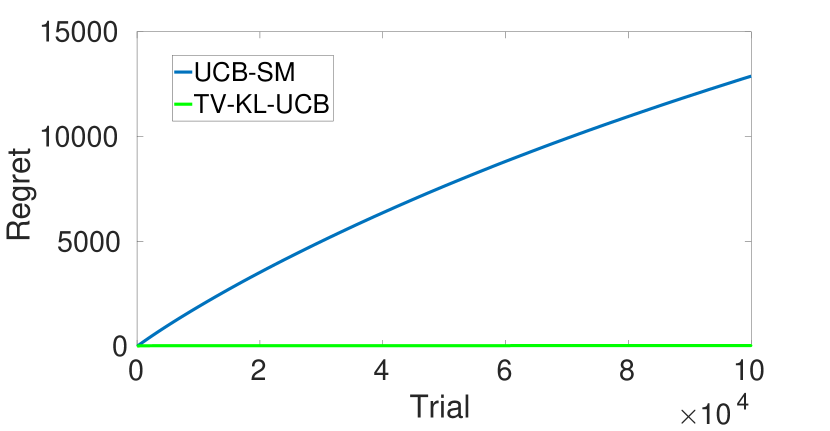
(a)

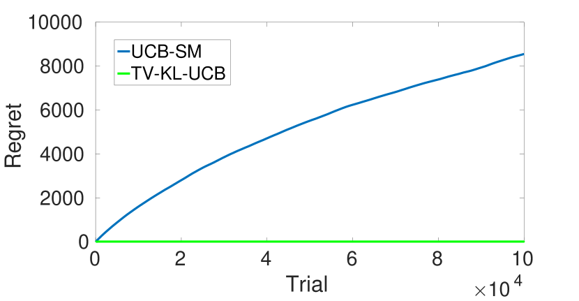
(b)

(c)

(d)

(e)

Figure 1: Comparison of regrets of different algorithms: UCB-SM and TV-KL-UCB: ((a) scenario 1, (b) scenario 2); KL-UCB-SM, KL-UCB-SM2 and TV-KL-UCB: ((c) scenario 1, (d) scenario 2); (e) regret upper bounds on TV-KL-UCB and UCB-SM.

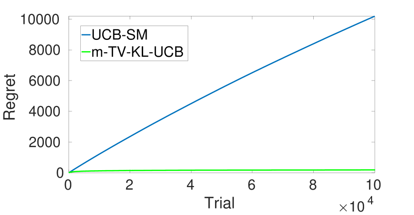
(a)

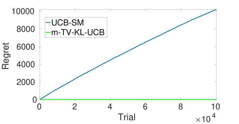
(b)

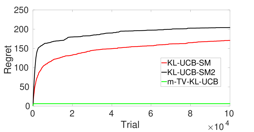
(c)

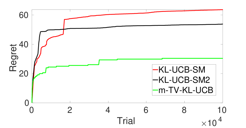
(d)

Figure 2: Comparison of regrets of different algorithms for scenarios 3 and 4.

In this section, we compare the performances of TV-KL-UCB and m-TV-KL-UCB with UCB-SM [10]. We also consider an improvement over [10] (referred to as KL-UCB-SM [8]) by replacing the UCB on sample mean by KL-UCB. Arm $A_{t}$ is chosen at time $t$ using the following scheme:
$A_{t}=\arg\max\limits_{i}\max\{\tilde{\mu}:D({\hat{\mu}}^{i}(t-1)||\tilde{\mu})\leq\frac{\log f(t)}{T_{i}(t-1)}\}.$ KL-UCB-SM2 is a modification of the algorithm in [13] when only one arm can be played at a time. We consider two scenarios and average the result over 100 runs. The code is available at https://github.com/arghyadip89/TV-KL-UCB.
Scenario 1: $p_{01}^{1}=0.5,p_{01}^{2}=0.4,p_{01}^{3}=0.3,p_{01}^{4}=0.2,p_{01}^{5}=0.1,p_{10}^{1}=0.4,p_{10}^{2}=0.55,p_{10}^{3}=0.65,p_{10}^{4}=0.65,p_{10}^{5}=0.7$.

Scenario 2: $p_{01}^{1}=0.5,p_{01}^{2}=0.0004,p_{01}^{3}=0.0003,p_{01}^{4}=0.0002,p_{01}^{5}=0.0001,p_{10}^{1}=0.4,p_{10}^{2}=0.00055,p_{10}^{3}=0.00065,p_{10}^{4}=0.00065,p_{10}^{5}=0.0007$.

In the first scenario (Fig. 1(a) and 1(c)), TV-KL-UCB significantly outperforms other algorithms. As KL-UCB provides a tighter confidence bound than UCB, the amount of exploration reduces. Since TV-KL-UCB identifies the best arm using estimates of $p_{10}^{i}$, $p_{01}^{i}$ in a truly Markovian setting, it spends lesser time in exploration than KL-UCB-SM and KL-UCB-SM2 which work based on the sample mean. In the second scenario, $p_{01}^{i}$ and $p_{10}^{i}$ for $i\neq 1$ are close to zero. As a result, the suboptimal arms spend a considerable amount of time in their initial states. If the initial estimates of $p_{10}^{i}$ and $p_{01}^{i}$ are taken to be zero, then the index of a suboptimal arm remain $1$ if it starts at state $0$ (see Equation (1)) until it makes a transition to state $1$. Therefore, our scheme may lead to a large regret in the beginning until all arms observe a transition to state $1$. To address this issue, we initialize $\hat{p}_{10}^{i}$ and $\hat{p}_{01}^{i}$ to $1$. We observe in Fig. 1(b) and 1(d) that TV-KL-UCB performs significantly better than UCB-SM, KL-UCB-SM and KL-UCB-SM2. Note that initial values of $\hat{p}_{10}^{i}$ and $\hat{p}_{01}^{i}$ do not play much role in the first scenario since each arm makes transitions from one state to another comparably often. The asymptotic upper bound on the regret of TV-KL-UCB is smaller than that of UCB-SM when $\min_{i}\sigma_{i}\geq\frac{1}{1440}$ (See Theorem 2). We choose parameters to satisfy $\min_{i}\sigma_{i}<\frac{1}{1440}$ and observe in Fig. 1(e) that still the asymptotic upper bound on the regret of TV-KL-UCB is better. For the i.i.d. case, the asymptotic upper bounds on the regrets of both KL-UCB-SM and TV-KL-UCB match the corresponding lower bound [8].

We also compare the performance of m-TV-KL-UCB with other algorithms when each arm is a three-state Markov chain with $r(0)=0,r(1)=1/2$ and $r(2)=1$. Similar to Scenarios 1 and 2, we consider two scenarios.
Scenario 3: $p_{01}^{1}=0.5,p_{01}^{2}=0.4,p_{01}^{3}=0.3,p_{01}^{4}=0.2,p_{01}^{5}=0.1,p_{02}^{1}=0.1,p_{02}^{2}=0.2,p_{02}^{3}=0.3,p_{02}^{4}=0.2,p_{02}^{5}=0.7,p_{12}^{1}=0.4,p_{12}^{2}=0.55,p_{12}^{3}=0.5,p_{12}^{4}=0.55,p_{12}^{5}=0.7,p_{10}^{1}=0.3,p_{10}^{2}=0.2,p_{10}^{3}=0.25,p_{10}^{4}=0.25,p_{10}^{5}=0.15,p_{20}^{1}=0.6,p_{20}^{2}=0.5,p_{20}^{3}=0.4,p_{20}^{4}=0.3,p_{20}^{5}=0.2,p_{21}^{1}=0.1,p_{21}^{2}=0.2,p_{21}^{3}=0.4,p_{21}^{4}=0.5,p_{21}^{5}=0.6.$

Scenario 4: $p_{01}^{1}=0.005,p_{01}^{2}=0.004,p_{01}^{3}=0.003,p_{01}^{4}=0.002,p_{01}^{5}=0.1,p_{02}^{1}=0.001,p_{02}^{2}=0.002,p_{02}^{3}=0.003,p_{02}^{4}=0.002,p_{02}^{5}=0.7,p_{12}^{1}=0.004,p_{12}^{2}=0.0055,p_{12}^{3}=0.005,p_{12}^{4}=0.0055,p_{12}^{5}=0.7,p_{10}^{1}=0.003,p_{10}^{2}=0.002,p_{10}^{3}=0.0025,p_{10}^{4}=0.0025,p_{10}^{5}=0.15,p_{20}^{1}=0.006,p_{20}^{2}=0.005,p_{20}^{3}=0.004,p_{20}^{4}=0.003,p_{20}^{5}=0.2,p_{21}^{1}=0.001,p_{21}^{2}=0.002,p_{21}^{3}=0.004,p_{21}^{4}=0.005,p_{21}^{5}=0.6.$

In both the scenarios, m-TV-KL-UCB performs better than other algorithms as KL-UCB provides a tighter confidence bound than UCB (See Figs 2(a), 2(b),2(c), 2(d)). Moreover, in truly Markovian settings, as considered by us, m-TV-KL-UCB picks the correct variant of KL-UCB frequently contrary to other algorithms such as KL-UCB-SM and KL-UCB-SM2 which work based on the sample mean. The performance improvement achieved by m-TV-KL-UCB is more than that of TV-KL-UCB as the incorrect variant of KL-UCB leads to more regret when the number of states is more.

5 Discussions & Conclusions

TV-KL-UCB uses the total variation distance between empirical estimates of $p_{01}^{i}$ and $(1-p_{10}^{i})$ to switch from STP_PHASE to SM_PHASE. Arm $i$ can be represented uniquely using $p_{01}^{i}$ and $p_{10}^{i}$. However, for i.i.d. rewards, it can be represented uniquely using the mean reward. Therefore, usage of STP_PHASE for i.i.d. arms may lead to a large regret since the additional information (which can be exploited by the sample mean based KL-UCB) is not exploited. We design the algorithm so that it works well for both scenarios. When the arms are i.i.d. (truly Markovian), the SM_PHASE (STP_PHASE) is chosen infinitely often. Theoretical (under a mild assumption) and experimental results show that the asymptotic upper bound on the regret of TV-KL-UCB is lower than that of UCB-SM [10]. In the i.i.d. case, the upper bounds on the regrets of KL-UCB-SM and TV-KL-UCB match the lower bound. For TV-KL-UCB, to overcome the issue of high regret associated with zero initialization, we initialize $\hat{p}_{01}$ and $\hat{p}_{10}$ to $1$. Experiments establish that the extension of TV-KL-UCB to a multi-state Markovian model outperforms other algorithms.

To conclude, in this paper, we have designed algorithms which achieve a significant improvement over state-of-the-art bandit algorithms. The idea is to detect whether the arm reward is truly Markovian or i.i.d. using a total variation distance based test. It switches from the standard KL-UCB to a sample transition probability based KL-UCB when it detects that the arm reward is truly Markovian. Logarithmic upper bounds on the regret of the algorithm have been derived for i.i.d. and Markovian settings. The upper bound on the regret of TV-KL-UCB matches the lower bound for i.i.d arm rewards.

6 Lower Bound on Regret of a Uniformly Good Policy

We derive a lower bound on the regret associated with any uniformly good policy. It is easy to verify that the lower bound matches with the lower bound in [11]. Note that unlike [11], we do not assume that the transition functions belong to a single-parameter family. Therefore, the lower bound derived in this paper is applicable to a larger class of transition functions (class of irreducible Markov chains) than [11].

Theorem 3.

For a uniformly good policy $\alpha$,

$$\liminf\limits_{n\to\infty}\frac{R_{\alpha}(n)}{\log n}\geq\sum\limits_{i=2}^{K}\frac{\Delta_{i}}{I(M_{i}||M_{1})}.$$

Proof.

We assume that the arm played and the reward obtained at time $t$ is denoted by $i_{t}$ and $r_{i_{t}}$, respectively. Let $F_t=\{i_1,r_{i_1},\mathrm{\dots },i_{t-1},r_{i_{t-1}}\}$

References

- [1] H. Robbins, “Some aspects of the sequential design of experiments,” Bulletin of the American Mathematical Society, vol. 58, no. 5, pp. 527–535, 1952.
- [2] T. L. Lai and H. Robbins, “Asymptotically efficient adaptive allocation rules,” Advances in applied mathematics, vol. 6, no. 1, pp. 4–22, 1985.
- [3] P. Auer, N. Cesa-Bianchi, Y. Freund, and R. E. Schapire, “The nonstochastic multiarmed bandit problem,” SIAM journal on computing, vol. 32, no. 1, pp. 48–77, 2002.
- [4] W. R. Thompson, “On the likelihood that one unknown probability exceeds another in view of the evidence of two samples,” Biometrika, vol. 25, no. 3/4, pp. 285–294, 1933.
- [5] V. Anantharam, P. Varaiya, and J. Walrand, “Asymptotically efficient allocation rules for the multiarmed bandit problem with multiple plays-part i: IID rewards,” IEEE Transactions on Automatic Control, vol. 32, no. 11, pp. 968–976, 1987.
- [6] R. Agrawal, “Sample mean based index policies by regret for the multi-armed bandit problem,” Advances in Applied Probability, vol. 27, no. 4, pp. 1054–1078, 1995.
- [7] P. Auer, N. Cesa-Bianchi, and P. Fischer, “Finite-time analysis of the multiarmed bandit problem,” Machine learning, vol. 47, no. 2-3, pp. 235–256, 2002.
- [8] A. Garivier and O. Cappé, “The KL-UCB algorithm for bounded stochastic bandits and beyond,” in conference on learning theory, 2011, pp. 359–376.
- [9] O. Cappé, A. Garivier, O.-A. Maillard, R. Munos, and G. Stoltz, “Kullback–Leibler upper confidence bounds for optimal sequential allocation,” The Annals of Statistics, vol. 41, no. 3, pp. 1516–1541, 2013.
- [10] C. Tekin and M. Liu, “Online algorithms for the multi-armed bandit problem with Markovian rewards,” in IEEE Annual Allerton Conference on Communication, Control, and Computinga, 2010, pp. 1675–1682.
- [11] V. Anantharam, P. Varaiya, and J. Walrand, “Asymptotically efficient allocation rules for the multiarmed bandit problem with multiple plays-part ii: Markovian rewards,” IEEE Transactions on Automatic Control, vol. 32, no. 11, pp. 977–982, 1987.
- [12] C. Tekin and M. Liu, “Online learning of rested and restless bandits,” IEEE Transactions on Information Theory, vol. 58, no. 8, pp. 5588–5611, 2012.
- [13] V. Moulos, “Finite-time analysis of round-robin kullback-leibler upper confidence bounds for optimal adaptive allocation with multiple plays and markovian rewards,” Advances in Neural Information Processing Systems, vol. 33, pp. 7863–7874, 2020.
- [14] H. Liu, K. Liu, and Q. Zhao, “Learning in a changing world: Restless multiarmed bandit with unknown dynamics,” IEEE Transactions on Information Theory, vol. 59, no. 3, pp. 1902–1916, 2012.
- [15] C. Tekin and M. Liu, “Online learning in opportunistic spectrum access: A restless bandit approach,” in IEEE INFOCOM, 2011, pp. 2462–2470.
- [16] C. Cortes, G. DeSalvo, V. Kuznetsov, M. Mohri, and S. Yang, “Discrepancy-based algorithms for non-stationary rested bandits,” arXiv preprint arXiv:1710.10657, 2017.
- [17] T. Graepel, J. Q. Candela, T. Borchert, and R. Herbrich, “Web-scale bayesian click-through rate prediction for sponsored search advertising in microsoft’s bing search engine.” Omnipress, 2010.
- [18] R. Herbrich, T. Minka, and T. Graepel, “Trueskill™: A bayesian skill rating system,” in Proceedings of the 19th international conference on neural information processing systems, 2006, pp. 569–576.
- [19] T. Lattimore and C. Szepesvári, “Bandit algorithms,” preprint, 2018.
- [20] V. Avadhanula, R. Colini Baldeschi, S. Leonardi, K. A. Sankararaman, and O. Schrijvers, “Stochastic bandits for multi-platform budget optimization in online advertising,” in WWW, 2021, pp. 2805–2817.
- [21] R. Zheng and C. Hua, Sequential Learning and Decision-Making in Wireless Resource Management. Springer, 2016.
- [22] J. Gittins, “A dynamic allocation index for the sequential design of experiments,” Progress in statistics, pp. 241–266, 1974.
- [23] P. Whittle, “Restless bandits: Activity allocation in a changing world,” Journal of applied probability, vol. 25, no. A, pp. 287–298, 1988.
- [24] A. Lazaric, E. Brunskill et al., “Online stochastic optimization under correlated bandit feedback,” in International Conference on Machine Learning. PMLR, 2014, pp. 1557–1565.
- [25] D. P. Foster and R. Vohra, “Regret in the on-line decision problem,” Games and Economic Behavior, vol. 29, no. 1-2, pp. 7–35, 1999.
- [26] N. Cesa-Bianchi and G. Lugosi, Prediction, learning, and games. Cambridge university press, 2006.
- [27] O. Besbes, Y. Gur, and A. Zeevi, “Stochastic multi-armed-bandit problem with non-stationary rewards,” Advances in neural information processing systems, vol. 27, pp. 199–207, 2014.
- [28] T. Jaksch, R. Ortner, and P. Auer, “Near-optimal regret bounds for reinforcement learning.” Journal of Machine Learning Research, vol. 11, no. 4, 2010.
- [29] M. G. Azar, I. Osband, and R. Munos, “Minimax regret bounds for reinforcement learning,” in International Conference on Machine Learning. PMLR, 2017, pp. 263–272.
- [30] R. Fruit, M. Pirotta, and A. Lazaric, “Near optimal exploration-exploitation in non-communicating markov decision processes,” arXiv preprint arXiv:1807.02373, 2018.
- [31] O. Cappé, A. Garivier, R. Munos, and G. Stoltz, “Supplement to “Kullback–Leibler upper confidence bounds for optimal sequential allocation,” 2013.
- [32] J. Lin, “Divergence measures based on the Shannon entropy,” IEEE Transactions on Information theory, vol. 37, no. 1, pp. 145–151, 1991.
- [33] R. Agrawal, “Finite-sample concentration of the multinomial in relative entropy,” IEEE Transactions on Information Theory, vol. 66, no. 10, pp. 6297–6302, 2020.
- [34] S. S. Dragomir, M. Scholz, and J. Sunde, “Some upper bounds for relative entropy and applications,” Computers & Mathematics with Applications, vol. 39, no. 9-10, pp. 91–100, 2000.