A Wideband Polarization Study of Cygnus A with the JVLA. I: The Observations and Data

Abstract

We present results from deep, wideband, high spatial and spectral resolution observations of the nearby luminous radio galaxy Cygnus A with the Jansky Very Large Array. The high surface brightness of this source enables detailed polarimetric imaging, providing images at $0.75\arcsec$, spanning 2 - 18 GHz, and at 0.30$\arcsec$ (6 - 18 GHz). The fractional polarization from 2000 independent lines of sight across the lobes decreases strongly with decreasing frequency, with the eastern lobe depolarizing at higher frequencies than the western lobe. The depolarization shows considerable structure, varying from monotonic to strongly oscillatory. The fractional polarization in general increases with increasing resolution at a given frequency, as expected. However, there are numerous lines of sight with more complicated behavior. We have fitted the $0.3\arcsec$ images with a simple model incorporating random, unresolved fluctuations in the cluster magnetic field to determine the high resolution, high-frequency properties of the source and the cluster. From these derived properties, we generate predicted polarization images of the source at lower frequencies, convolved to 0.75$\arcsec$. These predictions are remarkably consistent with the observed emission. The observations are consistent with the lower-frequency depolarization being due to unresolved fluctuations on scales $\gtrsim$ 300 - 700 pc in the magnetic field and/or electron density superposed on a partially ordered field component. There is no indication in our data of the location of the depolarizing screen or the large-scale field, either, or both of which could be located throughout the cluster, or in a boundary region between the lobes and the cluster.

1 Introduction

Cygnus A (3C 405) is the prototypical Fanaroff-Riley type II radio galaxy (Fanaroff & Riley, 1974). It is one of the most luminous radio galaxies known, and is exceptionally close ($z=0.056$; Spinrad & Stauffer, 1982) compared to galaxies of similar radio luminosity (see Fig. 1 of Stockton & Ridgway, 1996). Cygnus A’s high flux density ($\sim 1000$ Jy at $2$ GHz), combined with its relatively small angular size (maximum projected extent of $\approx$ $120\arcsec$) means the source is unusually bright, making it an outstanding target for high resolution radio polarimetric imaging with synthesis telescopes like the Very Large Array (VLA).

Cygnus A is located at the center of a dense cooling-core X-ray emitting cluster (Giacconi et al., 1972; Fabbiano et al., 1979). The cluster has a core of radius $\sim 18$ kpc and density of $\sim 15\times 10^{-26}$ g cm^-3 (Smith et al., 2002; Halbesma et al., 2019). The gas temperature decreases from $\sim 9$ keV at $\sim 300$ kpc radius to $\sim 3.5$ keV within the core (see top right plot Fig. 4 in Snios et al., 2018). Cygnus A is surrounded by a weak cocoon shock, driven by the expanding lobes, extending $33$ kpc north and $74$ kpc west of the cluster center (Carilli et al., 1994; Snios et al., 2018), with Mach numbers ranging between $1.18-1.66$ across the shock.

Figure 1 shows the total intensity contours at $2$ GHz with $1\arcsec$ resolution superimposed on the Chandra X-ray image in the energy interval $0.5-7$ keV. The well-known structures in the radio and X-ray are labeled: the central nucleus, the lobes, the four hotspots and the radio jet, as well as filamentary structures across the lobes, a ring-like structure in the tail of the eastern lobe (Perley et al., 1984), and the X-ray ‘jet’ (de Vries et al., 2018), cocoon-shock (Snios et al., 2018) and ribs (Duffy et al., 2018).

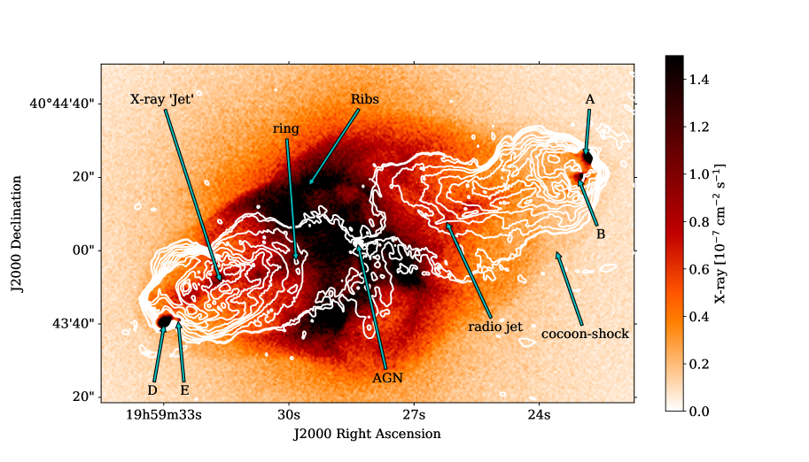
Figure 1: Chandra X-ray data ($0.5-7$ keV) of Cygnus A superimposed by the total intensity contour image ($2.4$ GHz and $1\arcsec$) of our new wideband data. The contour levels are $0.005$, $0.01$, $0.05$, $0.1$, $0.2$, $0.3$, $0.4$, $0.5$, $0.6$, $0.8$, $1.0$ Jy beam^-1. Shown are the radio features: the hot spots A, B, D and E at the ends of the lobes, the ring-like feature at the tails of the eastern lobe, the radio jet in the western lobe, and the central AGN. Also shown are the X-ray features: the X-ray jet, cocoon shock (the sheath) and the ribs (de Vries et al., 2018; Snios et al., 2018; Duffy et al., 2018). The off-source noise of the radio image is $1.7$ mJy beam^-1.

Cygnus A is significantly polarized with typical polarizations of $\lesssim 40\%$, and as high as $70\%$ in the lobes and hot spots at high resolution (Carilli et al., 1989). Polarimetric observations of Cygnus A showed large Faraday rotations across its lobes, asymmetry in the polarization properties of the lobes, as well as significant decreases in fractional polarization with decreasing frequency at low resolutions (Slysh, 1966; Mitton, 1971; Dreher, 1979; Alexander et al., 1984). The high resolution study by Dreher et al. (1987) revealed typical rotation measures, $RM$, ranging between $-4000$ $\mathrm{rad\,m}^{-2}\,$and $+3000$ $\mathrm{rad\,m}^{-2}\,$across the lobes, with gradients in the $RM$ distribution of $300$ $\mathrm{rad\,m}^{-2}\,$arcsecond^-1 in most parts of the lobes, and with a few places having gradients up to $1000$ $\mathrm{rad\,m}^{-2}\,$arcsecond^-1. These large gradients are responsible for the low polarization seen in the early low-resolution studies. The primary focus since then has been to understand the origin of these depolarizations and extraordinary Faraday rotations. The locations considered were our own galaxy, the X-ray cluster, the cocoon-shock, or a mixed thermal/synchrotron gas region located at the boundary of the lobes, or within the lobes themselves.

At the low galactic latitude of Cygnus A, $b=5.8^{\circ}$, our own galaxy contributes no more than $RM\sim 300$ $\mathrm{rad\,m}^{-2}\,$(Simard-Normandin et al., 1981), and consists of gradients not exceeding $180$ $\mathrm{rad\,m}^{-2}\,$between component separated by no more than $1^{\circ}$ (Clegg et al., 1992). Thus it was concluded that the origin of the large $RM$ and gradients must be local to the source (Dreher et al., 1987). Dreher et al., noting the high polarization at $6$ cm, the large total rotation of the electric vector (up to $600^{\circ}$ at that wavelength), and the apparently perfect linearity of the observed electric field position angle vs $\lambda^{2}$ between $6$ and $2$ cm wavelength, concluded that the great majority of the observed $RM$ must be due to an external medium, and cannot originate from a mixed thermal/synchrotron region inside the lobes. If the origin of the $RM$ is distributed throughout the cluster, the resulting magnetic fields were inferred to be $\sim 5$ $\mu$G. If the origin were confined to the cocoon-shock, the fields would be $\sim 20$ times higher.

A cluster origin for the majority of the $RM$ does not exclude smaller contributions from the cocoon-shock. Carilli et al. (1988), discovering a region of enhanced $RM$ in front of hotspot ‘D’ of the western lobe, suggested that both the cluster gas and the cocoon-shock contribute, with the cocoon-shock responsible for $|RM|\leq 1000$ $\mathrm{rad\,m}^{-2}\,$ordered on scales $<5$ kpc while the cluster is responsible for $|RM|>1000$ $\mathrm{rad\,m}^{-2}\,$ordered on scales $>\,20$ kpc.

Dreher et al.’s results were based on only four wavelengths spanning $\lambda$ $6$ cm to $2$ cm. Subtle depolarization effects, such as those due to turbulence or to boundary layer effects will not be visible with such sparse sampling. Since depolarization effects due to Faraday rotation are manifested at lower frequencies, investigation of such mechanisms require observations at frequencies below 5 GHz, with continuous frequency coverage. With the completion of the wideband Jansky Very Large Array (JVLA, Perley et al., 2001), we have now the capability to observe Cygnus A at lower frequencies than those available to Dreher et al., – notably, use of the new $2$ – $4$ GHz receiver – and with complete frequency coverage.

In this paper we present the results of our new wideband ($2$ – $18$ GHz), full polarization and high-spectral resolution observations of Cygnus A taken with the JVLA. The primary science goals of this study are to determine the spatial and frequency dependence of the depolarization, identify the physical structures and conditions responsible for this depolarization, and to determine the structures in the magnetic fields of the source and the surrounding cluster.

The results are presented in two papers: this paper presents the observations and primary data products, and results from analysis of the high frequency data. The second paper will present results from our modeling of the wideband data, and physical interpretations from this modeling.

This paper is organized as follows: The observations and calibration of the data are presented in section 2; and the imaging of the data in section 3. Section 4 presents our polarization results, followed by the results of a high-frequency high-resolution Faraday rotation study in section 5. In section 6 we show the results of applying the high frequency, high resolution model to the low frequency data. A summary and discussion are in section 7.

2 Observations and Calibration

The observations were taken under VLA observing project 14B-336. The details of these observations are shown in Table 1. This project utilized all array configurations for four observing bands; 2 – 4 GHz (‘S-band’), 4 – 8 GHz (’C-band’), 8 – 12 GHz (‘X-band’), and 12 – 18 GHz (‘Ku-band’), providing complete frequency coverage from $2$ to $18$ GHz.

Table 1: Observing log

Configuration	Date	Band	IAT Range	TOS	LST Range
			[H:M]	[min]	[H:M]
D	2015 Nov 15	S	20:09 - 01:96	20	16:40 - 22:20
	2015 Nov 15	C	20:09 - 01:96	40	16:40 - 22:20
	2015 Nov 15	X	20:09 - 01:96	60	16:40 - 22:20
	2015 Nov 15	Ku	20:09 - 01:96	95	16:40 - 22:20
C	2014 Nov 03	S	18:10 - 04:40	105	14:00 - 00:15
	2014 Nov 03	C	18:10 - 04:40	100	18:10 - 04:40
	2014 Nov 03	X	18:10 - 04:40	100	18:10 - 04:40
	2014 Nov 03	Ku	18:10 - 04:40	125	18:10 - 04:40
B	2015 Apr 05	S	09:15 - 16:50	130	15:10 - 22:30
	2015 Apr 12	C	10:00 - 17:35	130	16:25 - 23:30
	2015 Apr 12	X	10:00 - 17:35	180	16:25 - 23:30
	2015 Apr 05	Ku	09:15 - 16:50	185	15:10 - 22:30
A	2015 Aug 15	S	03:00 - 10:30	390	16:40 - 00:00
	2015 Jul 15	C	04:25 - 11:55	370	17:00 - 00:15
	2015 Jul 14	X1	04:25 - 11:42	350	16:40 - 00:00
	2015 Aug 11	X2	01:00 - 08:25	365	15:10 - 22:30
	2015 Jun 29	Ku	03:40 - 11:15	370	15:10 - 22:35

The correlator was configured to span the entire frequency range for each band. To facilitate data editing (primarily for RFI), the time averaging was set to $2$ seconds, and the channel width to $2$ MHz for C, X, and Ku bands, and to $1$ MHz at S band. Following editing and calibration, the data were time- and frequency-averaged, as described below.

A standard observing regimen was utilized – a nearby calibrator, J2007+4029 was observed periodically to monitor system health and to provide both complex gain and antenna cross-polarization calibration. At S-band in D-configuration, the visibility from Cygnus significantly perturbs observations of J2007+4029, so the more distant, but weaker, calibrator J2023+5427, was utilized for that band and configuration.

All data reduction was done using the Astronomical Image Processing System (AIPS) software package. The procedures followed were standard, and only a brief summary is given below:

1. To reduce spectral ringing due to RFI signals, the visibilities were Hanning smoothed.

2. Antennas which are shadowed at low observing elevations were identified and flagged.

3. Data corrupted by system failures or RFI were identified and removed.

4. Delay and bandpass calibration for each antenna was done using 3C286.

5. The flux densities of J2007+4029 or J2023+5427 were established by bootstrapping from 3C286.

6. The complex gains were computed from the calibrators and applied to all sources.

7. The cross-hand delays were found using 3C286, and applied to all sources.

8. Antenna cross-polarization (D-terms) were computed using the calibrator observations, and applied.

9. The cross-hand phase (to set the position angle of the linearly polarized flux) was determined from observations of 3C286, and applied to all sources.

Following these procedures the data were then averaged in time and frequency to generate the databases actually used in the imaging. The time and frequency averaging employed varied with the observing band as described below.

Time averaging reduces the visibility amplitude due to phase rotation of a source which is offset from the phase tracking center. We adopted a criterion of a maximum loss of $10\%$ on the longest baseline for a point source offset by $70\arcsec$ – the location of the western hotspot with respect to the nucleus. The resulting condition is

$$\delta t=\frac{\lambda}{4\,B_{\text{max}}\,\omega\,\chi}$$ (1)

where $B_{max}$ is the maximum baseline in meters, $\omega$ is the earth’s rotation rate in radians s^-1, $\chi$ is the offset in rad, and $\lambda$ is the observing wavelength in meters. For Cygnus A, and the $35$-km maximum baseline, the integration time is $22$, $11$, $7.1$ and $5$ seconds, for the S, C, X, and Ku-bands, respectively. We utilized $10$ seconds for S and C, $8$ seconds for X, and $6$ seconds for Ku bands. Note that since the hotspots are well resolved, the actual loss of brightness due to this effect will be considerably less than the 10% condition utilized.

There are two conditions which set the maximum tolerable channelwidth – chromatic aberration (bandwidth smearing), and polarization intensity reduction due to the rotation measure. We discuss these in turn:

1. Frequency averaging radially stretches the emission from a source, with increasing offset from the phase tracking center. We applied the same condition as for time averaging – that the longest baselines suffer a maximum of $10\%$ loss in amplitude for a point-source $70\arcsec$ from the nucleus. This results in the following:

   $$\delta\nu=\frac{c}{4\,B_{\text{max}}\,\chi}$$ (2)

   For the $70\arcsec$ offset of the western hotspot and the $35$-km maximum baselines, the maximum channel width is $6.3$ MHz. We adopted $8$ MHz. We note again that as the hotspots are well resolved on the longest baselines, the actual intensity loss is much less than the 10% criterion.

2. As discussed in Section 2, a linearly polarized EM wave, propagating through a magnetized ionized medium has its plane of polarization rotated by

   $$\Delta\chi=RM\lambda^{2}$$ (3)

   radians. Over a bandwidth $\delta\nu$, centered at frequency $\nu$, the rotation of the plane of polarization is given by

   $$\Delta\chi=2\lambda^{2}RM\frac{\delta\nu}{\nu}$$ (4)

   where it has been assumed that $\Delta\nu<<\nu$. The absolute value of the maximum $RM$ in Cygnus A is known to be $\sim 5000$ rad m^-2 (Dreher et al., 1987). With this value, and utilizing the stringent condition of a maximum of $10$ degrees rotation across a channel, the maximum channelwidth is $1.5$ MHz at $2$ GHz, $5.2$ MHz at $3$ GHz, and $12.4$ MHz at $4$ GHz. Hence, only at S-band is the polarization condition more stringent than the chromatic aberration condition. Thus, we adopted $2$ MHz for the lower half of S-band ($2$ – $3$ GHz), $4$ MHz for the upper half of S-band ($3$ – $4$ GHz), and $8$ MHz for all other bands.

This data compression process resulted in a database for each spectral window (spanning $64$ MHz at S-band, and $128$ MHz in all other bands) – hence $32$ channels for the lower half of S-band, and $16$ channels for all other bands in each spectral window and each configuration – a total of $498$ databases. These were then combined over configuration, resulting in 144 databases, each containing the data from all configurations for a single spectral window, from which the images were made.

Although Cygnus A has a very nearby calibrator, standard phase calibration alone results in image dynamic range (ratio of the brightest component to the rms noise) of less than $1000$ , far less than that needed for detailed imaging analysis. Fortunately, the high flux density of Cygnus A, combined with the ‘sharp’ features of the nucleus and hotspots, permits application of the technique of self-calibration (Cornwell & Wilkinson, 1981). To accomplish this, total intensity images of Cygnus A were generated from each of these decimated databases for each spectral window, utilizing a few central channels. These images were then used to self-calibrate the data to remove residual phase and gain fluctuations inherent in the process of calibration with an external calibrator. During this process, care was taken to ensure the unresolved nucleus was registered in the central (phase-tracking) cell, and that the total flux density of Cygnus A (following correction for the primary beam) equaled the values published by Perley, & Butler (2017). We believe the phase registration is accurate to $5$% of the full resolution at all bands, and that the flux density matches the Perley, & Butler (2017) scale to better than $2$%. The resulting images showed imaging dynamic ranges up to $30,000$:$1$ – more than an order of magnitude better than the initial images.

3 Imaging

Imaging was done using the AIPS software package, using the task IMAGR. We made Stokes $I$, $Q$ and $U$ image cubes using the multiscale cleaning deconvolution algorithm (Greisen, 2003; Cornwell, 2008; Greisen et al., 2009). The number of frequency planes utilized to prevent depolarization from the high $RM$ or from chromatic aberration, for each frequency band is shown in Table 3. In total, $1184$ frequency planes were used.

Table 2: The number of frequency planes in each band utilized to avoid Faraday depolarization.

Band	$\nu$-interval	$\Delta\nu$	$N_{avg}$	$N_{planes}$
	[GHz]	[MHz]
$\mathrm{S_{lo}}$	2-3	2	1	512
$\mathrm{S_{hi}}$	3-4	4	1	256
$\mathrm{C_{lo}}$	4-6	8	1	256
$\mathrm{C_{hi}}$	6-8	32	4	64
$\mathrm{X_{lo}}$	8-10	64	8	32
$\mathrm{X_{hi}}$–Ku	10-18	128	16	64

The image cubes were made at two standard resolutions: i) $0.75\arcsec$ resolution – corresponding to the highest resolution available at $2$ GHz (which thus includes all frequencies) and ii) $0.30\arcsec$ which corresponds to the highest resolution at $6$ GHz. All the images were primary beam corrected using the AIPS task ’PBCOR’.

The polarized intensity $P$ is a complex number, with amplitude given by $|P|=\sqrt{Q^{2}+U^{2}}$, and phase by

$$\chi=\frac{1}{2}\,\text{tan}^{-1}\bigg{(}\frac{U}{Q}\bigg{)}.$$ (5)

The amplitude was corrected for Ricean bias using the Maximum Likelihood approximation:

$$P_{\text{corr}}\approx P-\frac{0.5\,\sigma^{2}_{P}}{P}$$ (6)

where $\sigma_{P}$ is the error in $P$ (Killeen et al., 1986). We derived fractional polarizations by taking the following ratio

$$p=\frac{P_{\text{corr}}}{I}.$$ (7)

Errors associated with these quantities were derived assuming standard propagation of error formulae with the noise in $Q$, $U$ and $I$ estimated in an off-source region of each map. At 0.30$\arcsec$ the off-source noise ranges between 0.18 mJy beam^-1 and 0.5 mJy beam^-1 in Stokes $Q$, and $U$, and 0.3 mJy beam^-1 and 1 mJy beam^-1 in Stokes $I$. At 0.75$\arcsec$ the off-source noise ranges between 0.6 mJy beam^-1 and 1.6 mJy beam^-1 for Stokes $Q$ and $U$ images, and 0.8 mJy beam^-1 and 6 mJy beam^-1 for Stokes $I$ images.

We computed Faraday spectra, $\tilde{F}$, for every line of sight using the RM-synthesis technique as employed by Brentjens & de Bruyn (2005). We compute $\tilde{F}$ by summing the fractional polarized emission, $p$, over all $N$ channels as follows:

$$\tilde{F}(\phi)=\Bigg{(}\sum_{n=1}^{N}W_{n}\Bigg{)}^{-1}\sum_{n=1}^{N}\tilde{p}_{n}e^{-2i\phi(\lambda^{2}_{n}-\lambda^{2}_{0})},$$ (8)

where $\lambda^{2}_{n}$ is the wavelength squared of channel $n$, $W_{n}=W(\lambda^{2}_{n})$ is the weight of each channel, $\tilde{p}_{n}=W_{n}p_{n}$, $\lambda^{2}_{0}$ is a weighted offset in wavelength-squared space, and $\phi$ is Faraday depth, given by

$$\phi=810\int\limits_{z}^{0}n_{e}\mathbf{B}\cdot\mathrm{dz}\quad\quad[\mathrm{rad\,m}^{-2}].$$ (9)

Here, $\mathbf{B}$ is the magnetic field in $\mu$Gauss, $n_{e}$ is the electron density in $\mathrm{cm}^{-3}$, and $z$ is the pathlength in kpc. The derived $\tilde{F}$ is a ‘dirty’ spectrum; the true $F(\phi)$ convolved by the rotation measure transfer function, RMTF or $R(\phi)$:

$$R(\phi)=\Bigg{(}\sum_{n=1}^{N}W_{n}\Bigg{)}^{-1}\sum_{n=1}^{N}W_{n}e^{-2i\phi(\lambda^{2}_{n}-\lambda^{2}_{0})}.$$ (10)

The resolution of the RMTF is

$$\delta\phi\approx\frac{3.8}{\Delta\lambda^{2}}\quad\text{rad m${}^{-2}$},$$ (11)

where $\Delta\lambda^{2}=\lambda^{2}_{\text{max}}-\lambda^{2}_{\text{min}}$ is the width in the observed wavelength-squared space (Schnitzeler et al., 2009). For our data, $\delta\phi$ $\sim$175 rad m^-2 for 2 - 18 GHz, and $\delta\phi$ $\sim$1700 rad m^-2 for 6 - 18 GHz. Figure 2 shows the rotation measure transfer function for our data.

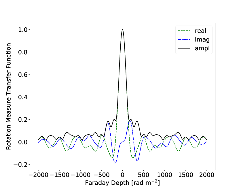
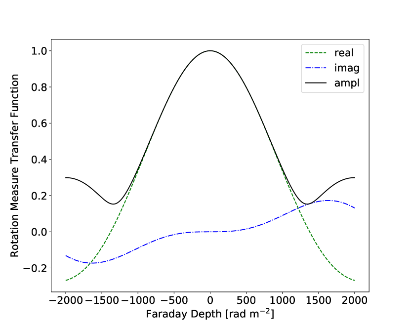
Figure 2: Rotation measure transfer functions of our data. Top is 2 - 18 GHz data, and bottom is 6 - 18 GHz.

The Faraday spectra shown in this paper were deconvolved using the cleaning algorithm presented by Heald (2009). We utilized both RM-synthesis and RM-clean provided in the AIPS task ‘TARS’. Our $\lambda^{2}$ sampling is non-uniform – resampling the data on a uniform grid did not alter the results in any significant way. We used uniform weighting, $W=1$, for all channels, and defined $\lambda^{2}_{0}$ as a weighted mean of the observed $\lambda^{2}$.

The maximum Faraday depth we can observe without significant attenuation is given by the phase rotation across a channel at the lowest frequency (see Eq. 4). An RM of 25000 rad m^-2 across a 2 MHz channel width at a frequency of 2 GHz will cause a rotation of 1 radian. Thus, the maximum RM in Cygnus A of $\sim$ 5000 rad m^-2 will suffer no appreciable attenuation. As noted by Brentjens & de Bruyn (2005), the short wavelength limit of the observations will limit the width of Faraday depths that can be recovered by Faraday synthesis for any given line of sight. Our minimum $\lambda^{2}$ of 3$\times$10^-4 m², would attenuate by 50% Faraday structures wider than 10000 rad m^-2 – far wider than those expected in Cygnus A.

4 Polarization Imaging of Cygnus A

Polarized emission of a source undergoing Faraday rotation can be used to study the properties of the medium causing the rotation. Distinguishing between various depolarization mechanisms can be difficult, and requires high resolution, low frequency observations. In this section, we show the polarization characteristics of Cygnus A as a function of resolution and frequency.

4.1 Polarization as a Function of Frequency

Figure 3 shows the $0.75\arcsec$ resolution maps of the fractional polarization across Cygnus A radio lobes at 10 GHz, 6 GHz, 4 GHz and 2 GHz. We show only those pixels with relative error in the fractional polarization, $(\sigma_{p}/p)\leq 0.5$. As seen in the figure, the fractional polarization of the lobes decreases significantly with decreasing frequency. Note that the eastern lobe depolarizes at higher frequencies than the western, and for both lobes, the depolarization is more rapid in the inner regions – those closer to the nucleus. The spatial distribution of the fractional polarization of the lobes is very uniform at high frequencies, with typical values of 20%, with some regions as high as 70%, and becomes clumpy on scales of $\sim 1$ kpc at low frequencies – most notably at 2 GHz. The fractional polarization at 2 GHz is less than 10% for virtually all lines of sight at this resolution. The emission from the bright hotspots, and from the jet, depolarizes in the same manner as that from the adjacent lobes. There is no correlation between the underlying source brightness or structure and the nature of the depolarization.

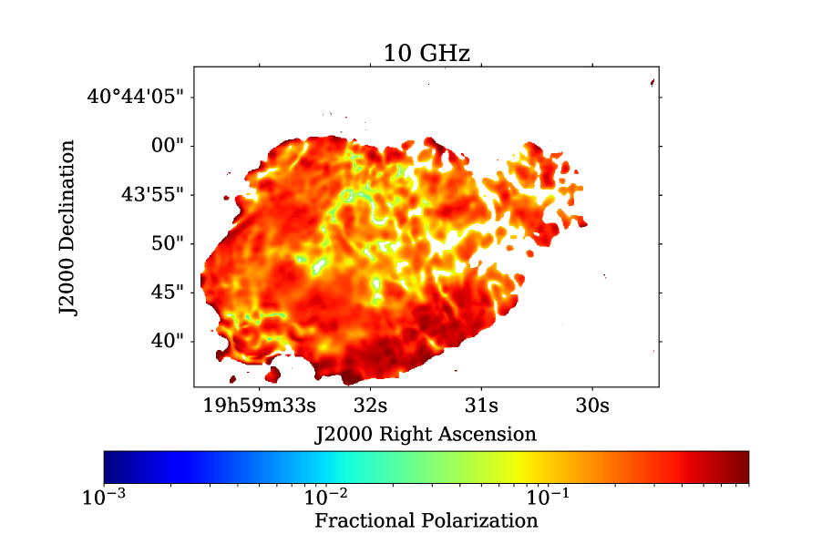
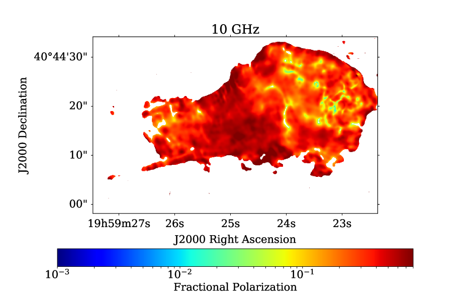
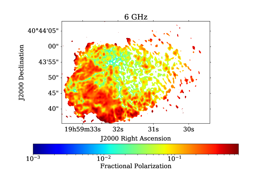
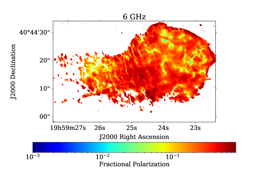
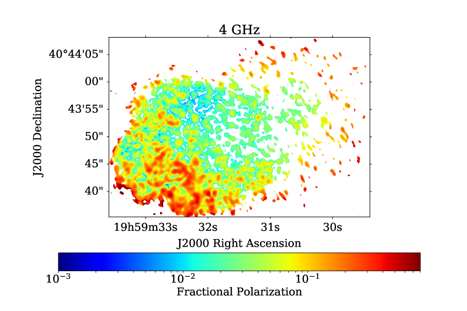
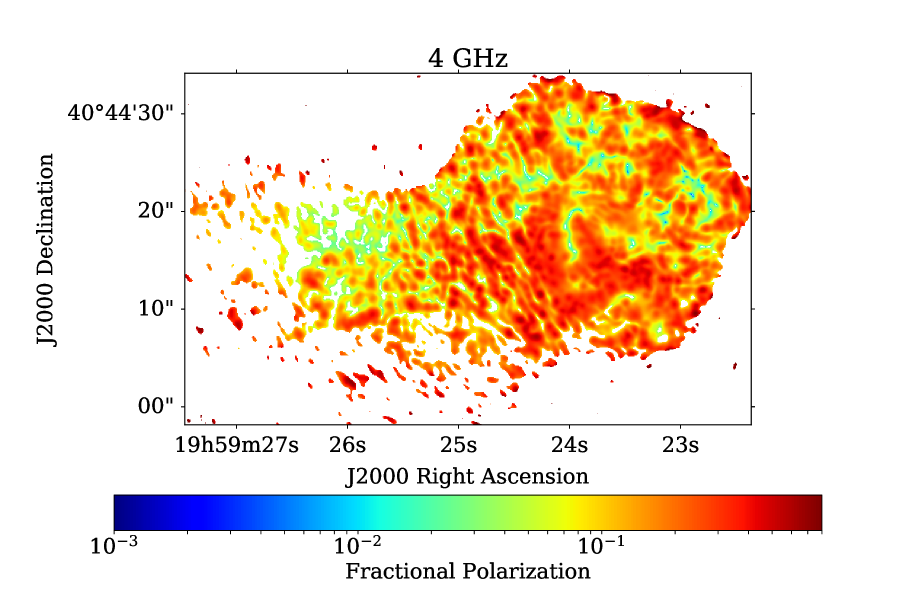
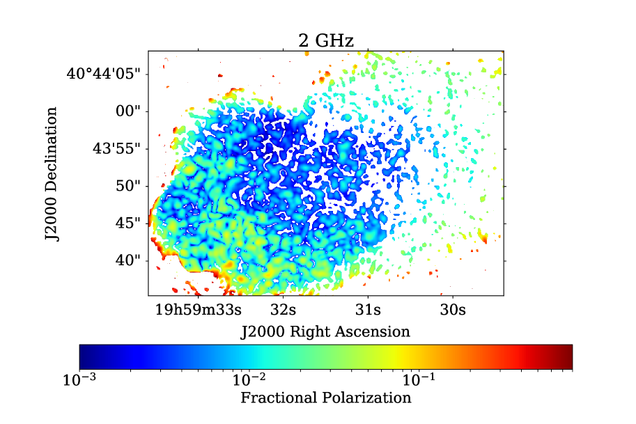
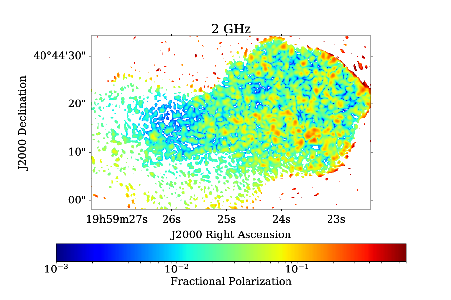
Figure 3: Fractional polarization maps of Cygnus A at $0.75\arcsec$ resolution at four different frequencies: $10$ GHz, $6$ GHz, $4$ GHz and $2$ GHz. The color-bar ranges between 0.1% and 80%. Only pixels with $(\sigma_{p}/p)<0.5$ are shown. There is a global decrease in fractional polarization with decreasing frequency. The eastern lobe depolarizes at higher frequency than the western. The inner regions (near the nucleus) of the lobes depolarize more rapidly than the outer regions.

The strong depolarization, and the very turbulent appearance of the low frequency fractional polarization images suggests that the depolarization may be related to partially-resolved fluctuations in the Faraday depth of the surrounding medium. To investigate this, we determined the dependence of the polarization as a function of frequency over our full bandwidth ($2-18$ GHz) at $0.75\arcsec$ resolution. This task is made challenging by the sheer quantity of information – over the solid angle subtended by the lobes, there are over $\sim 3000$ independent lines of sight. Thus, we can only show a few representative examples.

In order to efficiently identify specific lines of sight, we have defined a relative coordinate system, centered on the galaxy nucleus, with units of tens of milliarcseconds. Positive is to the west and north, and negative to the east and south. For example, a line of sight with coordinates (2444, -1024) is $22.44\arcsec$ west and $10.24\arcsec$ south of the nucleus. We analyze only those locations with error in the fractional polarization $<10\%$ at $8$ GHz. This resulted in a total of $2096$ independent lines of sight.

Figure 4 shows these depolarization functions for six representative lines of sight. Each row of three panels displays fractional polarization (Eq. 7) in the left panel, and the polarization position angle in the middle panel, all as functions of $\lambda^{2}$. The right panel shows the amplitude of the Faraday spectrum, superimposed in red is the Gaussian with width equal to that of the rotation measure transfer function (RMTF). The RMTF is shifted and scaled to match the location and amplitude of the maximum amplitude of the Faraday spectrum. Each line of sight is labeled according to the coordinate offsets defined above.

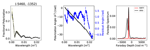
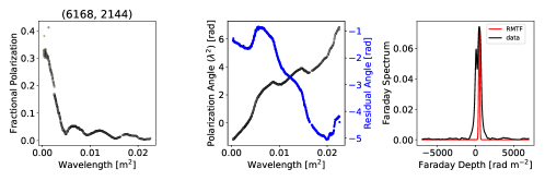
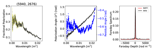
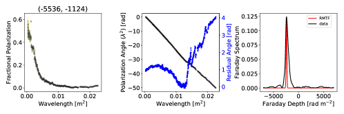
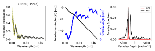
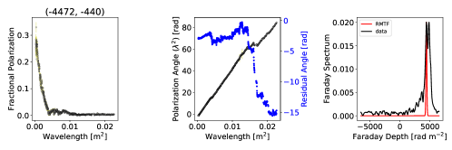
Figure 4: Fractional polarization from 2 to 18 GHz at $0.75\arcsec$ resolution for six representative locations. The left column shows the fractional polarization amplitude, the middle column the observed position angle (black) and the residual position angle (blue) after the dominant peak in the Faraday spectrum was removed. The right panel shows the amplitude of the Faraday spectrum (in black) with a Gaussian of width equal to that of the rotation measure transfer function (RMTF) superposed in red.

The fractional polarization of all lines of sight decreases significantly with increasing $\lambda^{2}$. For some lines of sight, the decrease is smooth, while for most, there is considerable structure in the depolarization, ranging from sharp nulls and peaks as shown in the top two rows of the figure, to more complex behaviors, as shown in the bottom two rows.

The polarization angle as a function of $\lambda^{2}$ of the data (shown in black) is plotted together with the residual angle (shown in blue) obtained by removing $RM_{\text{peak}}\lambda^{2}$ of the peak of the Faraday spectrum. The residual polarization angle, $\chi_{\text{res}}$, shows significant deviations; we find that 38% of the lines of sight have $0<\chi_{\text{res}}<\pi$, 22% have $\pi<\chi_{\text{res}}<3\pi$, 13% have $3\pi<\chi_{\text{res}}<6\pi$, 12% have $6\pi<\chi_{\text{res}}$, and the remaining 15% were noisy or the n$\pi$-ambiguity couldn’t be corrected. Lines of sight showing small deviations are usually associated with simple smooth decaying fractional polarizations with $\lambda^{2}$ or equivalently, with a single, nearly unresolved peak, similar to that shown on the third row of Fig. 4. The nonlinearities are more prominent when the fractional polarization vs. $\lambda^{2}$ behavior has structure such as in the oscillatory and complex cases.

The Faraday spectra show interesting structures – some lines of sight show a simple single peak, some have multiple peaks, and many lines of sight show a rather wide ‘base’, indicating a wide range of Faraday depths within the resolving beam. As expected, the depolarization curves with pronounced oscillations show multiple-peaked spectra, with the separation of the peaks typically $\lesssim 500$ $\mathrm{rad\,m}^{-2}\,$, and a maximum separation of $\sim 1500$ $\mathrm{rad\,m}^{-2}\,$(approximated by eye). The detailed characterization of Faraday spectra will be presented in paper 2.

To investigate whether these different depolarization functions have any spatial relationship, we generated a simple classification scheme based on the observed depolarization behavior. By viewing each fractional polarization as a function of $\lambda^{2}$ (left panel of Fig. 4), we classified by eye the lines of sight into three categories as follows:

1. ‘Sinc-like’ decay: the behavior in the decreasing fractional polarization as a function of increasing $\lambda^{2}$ is approximately that of a sinc function: $p\propto\sin(K\lambda^{2})/K\lambda^{2}$. The minima are sharp, and occur at nearly constant intervals, while the peaks decrease in amplitude towards large $\lambda^{2}$. Examples are shown in the top two rows in Fig. 4.

2. Smooth decay: the fractional polarization decreases smoothly with increasing $\lambda^{2}$ within measurement errors. Examples are shown in the third and fourth rows in Fig. 4.

3. Complex decay: the depolarization displays a combination of the above, or more complex behavior in the fractional polarization vs. $\lambda^{2}$. We further classified complex lines of sight into two sub-classes: ’complex-oscillatory’ and ’complex non-oscillatory’. The former resemble sinc-like pattern than smooth decay but the fractional polarization doesn’t approach 0 across $\lambda^{2}$ or the intervals are not periodic, or both, and the latter resemble smooth decay more than sinc-like but the decay is not completely smooth. See the last two rows in Fig. 4 for complex-oscillatory and non-oscillatory, respectively.

The fraction of lines of sight in each of these three classes are given the second column of Table 3. Moreover, column 3 to 7 gives a fraction of lines of sight with deviations in polarization angle (the residual angle, $\chi_{\text{res}}$) in each of the intervals: low ($0<\chi_{\text{res}}<\pi$), med ( $\pi<\chi_{\text{res}}<3\pi$), high ( $3\pi<\chi_{\text{res}}<6\pi$), and limit( $6\pi<\chi_{\text{res}}$), as well as a fraction of those that couldn’t be classified (denoted as ’N/A’). Most lines of sight are complex/intermediate – with the majority of the complex resembling smooth decays. In terms of the residual $\chi$, we find that decaying behavior without oscillations tend to have small deviations, while oscillatory structure results in slightly higher deviations.

Table 3: A fraction in % of lines of sight in different classes.

Class Name	Total	$\chi$- deviations						p($\lambda^{2}$) vs. $\theta$					Predictions
		Low	Med	High	Limit	N/A		class A	class B	class C	N/A		Good	Approx	N/A
sinc-like	11	30	42	17	7	4		36	16	46	2		8	73	19
smooth	25	70	14	8	4	4		35	22	40	3		13	72	15
complex osc	20	25	32	22	15	6		43	18	36	3		19	72	9
complex non-osc	30	40	24	14	13	9		38	20	40	2		17	70	13
complex (both)	50	33	28	18	14	7		40	19	38	3		18	71	11
All classifiable	86	41	28	15	10	6		38	19	40.5	2.5		14	72	14
Not class	14	-	-	-	-	-		-	-	-	-		-	-	-

Figure 5 shows a color-coded display of the distribution of these classifications across the lobes: lines of sight with sinc-like behavior are shown in red-orange (symbol x), smooth decay in green (o symbol), and complex decay in navy ($\ast$ symbol for oscillatory-like complex decay, and ’v’ symbol for non-oscillatory). The figure shows there are no clear spatial relationships for these behaviors, yet they are not completely random as adjacent cells are more likely to show the same behavior. These correlated ‘clumps’ are typically of a few kpc scale. There is a tendency for more complex behavior in the eastern lobes, and relatively fewer smooth decay and sinc-like behaviors. The distribution across the the western lobe, on the other hand, consists mostly of smooth decay particularly at the extremes of the lobes, and complex decay.

It should be noted that these classifications are only valid for this frequency span ($2-18$ GHz) and $0.75\arcsec$ resolution, and that the classes are likely to change with a change in spectral coverage or resolution.

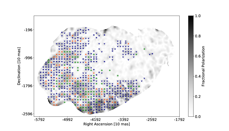
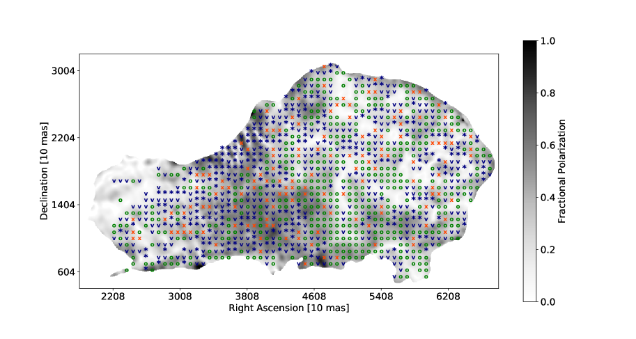
Figure 5: Lines of sight across each lobe classified based on the behavior of their fractional polarization vs. $\lambda^{2}$. The sinc-like behaviors are shown in red-orange with an ‘x’ symbol), smooth decay in green (’o’ symbol) and complex decay in navy ($\ast$ symbol for complex-oscillatory and ’v’ for complex non-oscillatory). The lines of sight are separated by the resolution beam of $0.75\arcsec$. These classes show no obvious large-scale spatial correlations. The majority ($50\%$) of the lines of sight show complex behavior, $25\%$ show smooth decay, and $11\%$ sinc-like.

4.2 Polarization as a Function of Spatial Resolution

The depolarization behavior shown in Section 4.1 can be explained by randomized fluctuations in the foreground Faraday screen on scales less than the $0.75\arcsec$ resolution. If this is the case, then the fractional polarization will in general decrease as the resolution decreases at any given frequency.

Figure 6 shows the fractional polarization at $4.0$ GHz of Cygnus A at four resolutions – $0.45\arcsec$, $0.75\arcsec$, $1.50\arcsec$ and $3.00\arcsec$. The resolution $0.45\arcsec$ is the highest we can obtain at this frequency. We show only pixels with $(\sigma_{p}/p)<50\%$. As expected, the fractional polarization decreases as the resolution degrades, most notably in the inner regions of the eastern lobe. The figure shows the effects of wavelength-dependent beam depolarization, as expected if the external medium is differentially rotating the polarized emission within the resolution element, as discussed below.

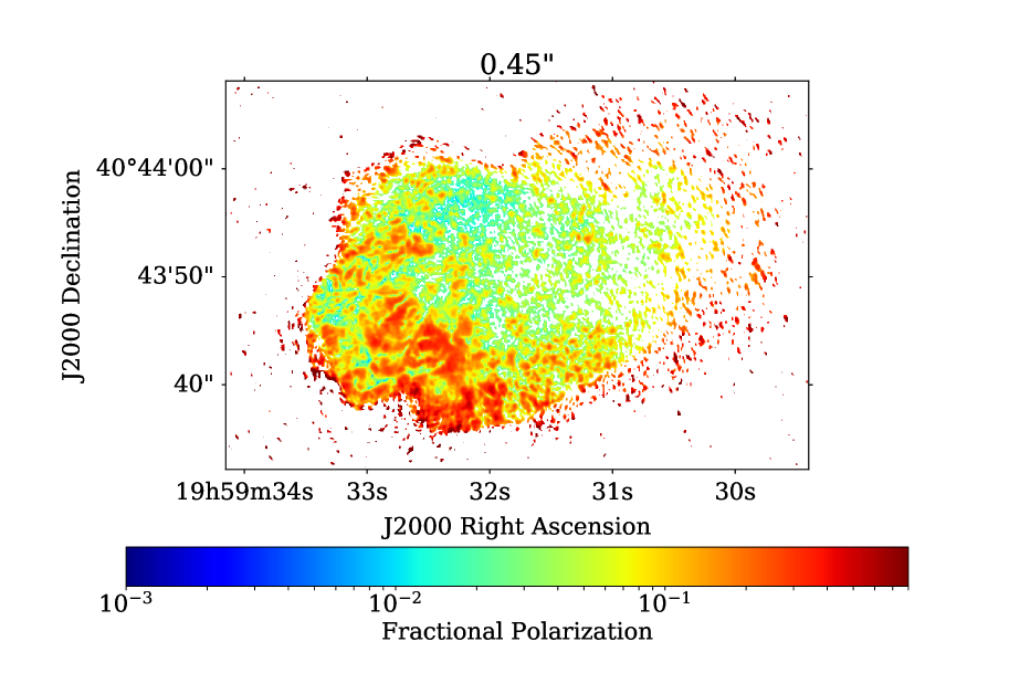
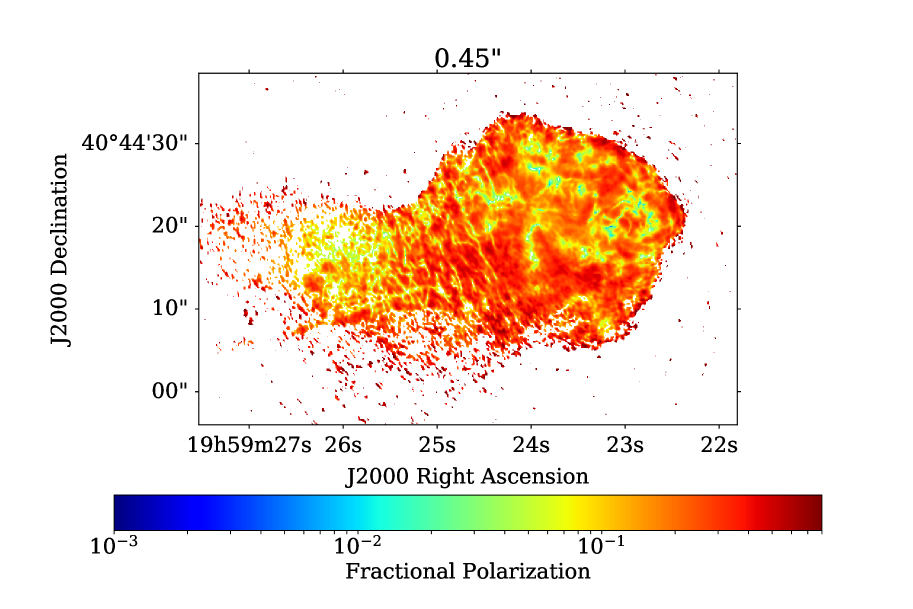
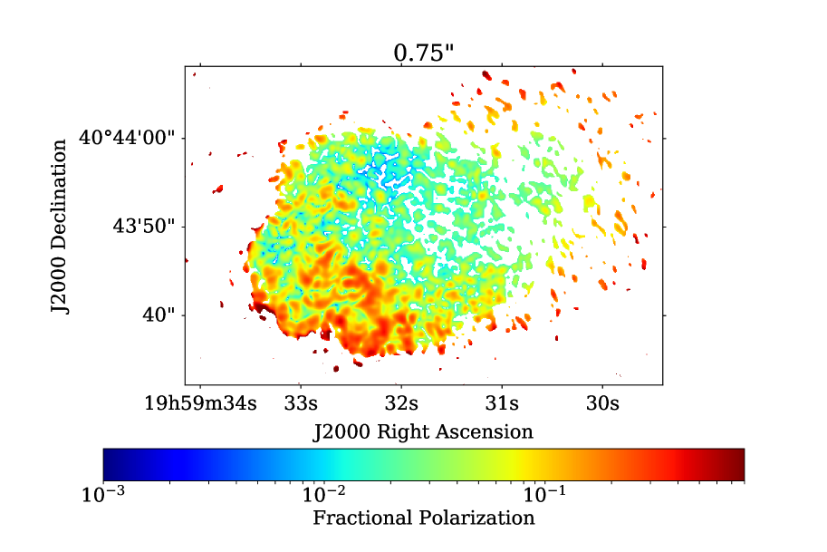
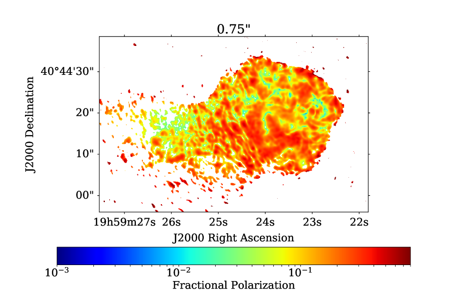
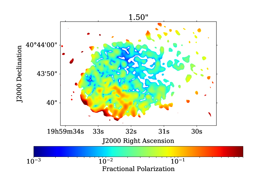
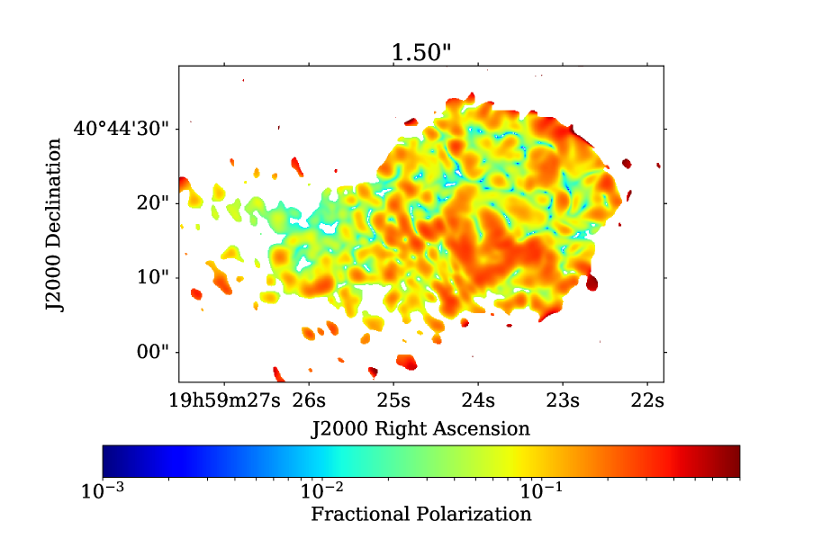
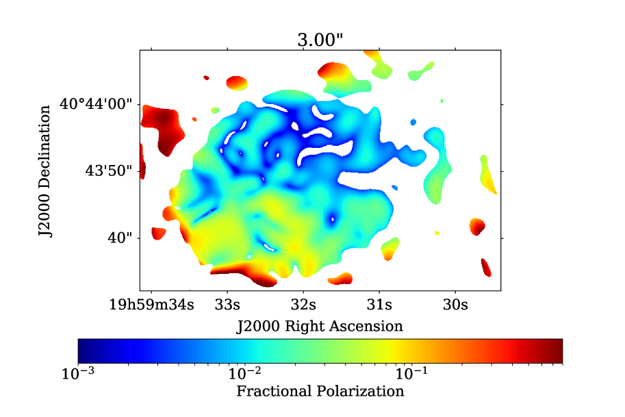
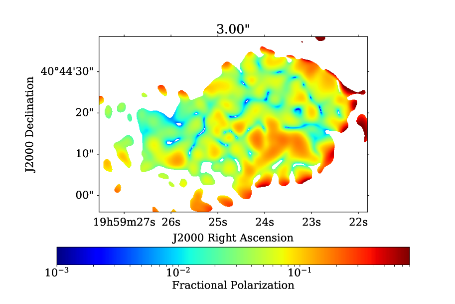
Figure 6: Fractional polarization maps at $4.0$ GHz at four different resolutions: $0.45\arcsec$ (top row), $0.75\arcsec$ (second row), $1.50\arcsec$ (third row), and $3\arcsec$ (bottom row). The color-bar ranges between 0.1% and 80%. Only pixels with $(\sigma_{p}/p)<50\%$ are shown. The fractional polarization decreases as the resolution degrades. This depolarization is higher in the eastern lobe especially in the region close to the galaxy.

If the depolarization is due to transverse fluctuations in the foreground screen, then at a resolution corresponding to smallest significant angular scale of the fluctuations, these structures will be resolved out, at which point the observed fractional polarization will be that of the source itself. If this intrinsic value can be established, any fractional polarization changes with frequency must then be due to intermixed thermal and synchrotron gas of the source itself, allowing an estimate of the thermal gas content. This is the only method known to us which can clearly discriminate between internal depolarization (i.e., within the lobes or a mixed boundary layer), and external depolarization (due to unresolved structures in the propagating medium).

Here we describe our efforts to determine the intrinsic value of the polarization by plotting the fractional polarization as a function of resolution ($\theta$) at five different frequencies, for $2096$ lines of sight. Figure 7 shows a few examples of the typical behavior. Each of the six panels shows the fractional polarization at $2$, $4$, $6$, $8$, and $10$ GHz as a function of resolution, from $3\arcsec$ to the highest permitted by the diffraction limit for given frequency, for different lines of sight through the lobes chosen to display the range of behavior. The left side shows three lines of sight where the behavior is close to the expected – a smooth rise in polarization with a flattening at sub-arcsecond resolutions. Note, however, that only in the top two is there any evidence for asymptotic behavior at the highest resolution. And even for these, the critical low frequency polarizations needed to establish whether there is internal depolarization do not have sufficient resolution to determine what the asymptotic values are.

The right hand panels show much more complex behavior, with structures in the depolarizing behavior which are likely due to structure of the fields in the emitting medium (i.e., the lobes), or the external depolarizing medium. We classified the lines of sight into three groups: i) those with fractional polarization which increases monotonically at least across four frequencies (class A), ii) those with non-monotonic behavior (class B) at four frequencies – this class also includes lines of sight with fractional polarization which decreases at higher resolutions, iii) and those whose fractional polarization vs. resolution behavior that differs for across the frequencies (class C). For example, left panel of Fig. 7 all fall into class A, the top two plots on the right panel fall into class B, and bottom-right plot fall into class C. This classification was done by eye. Column 7 to 11 of Table 3 gives the fraction of lines of sight in each of the above classes for different decaying behavior. We find that the same fraction (40%) of lines of sight are found in class A and C. Moreover, the classes do not seem to depend on the whether the line of sight is sinc-like, smooth decay, or complex.

It is clear that much higher resolutions – by at least an order of magnitude – are needed to be able to resolve out the beam depolarization effects, and permit an estimate of the true source polarization at the critical lower frequencies where depolarization phenomena are manifest. These plots emphasize that even with the VLA and its sub-kpc resolution, the responsible depolarizing mechanisms and underlying structures cannot be uniquely identified. A much larger instrument will be needed to finally clarify the processes responsible.

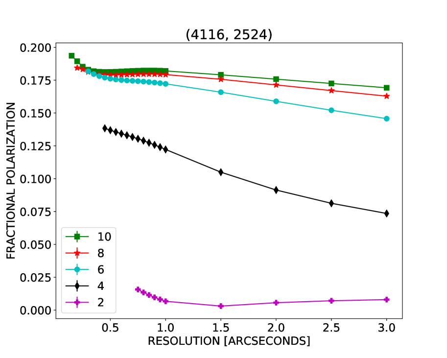
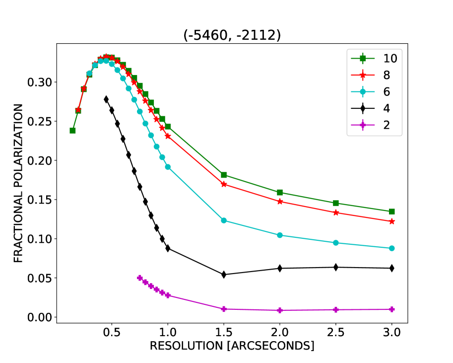
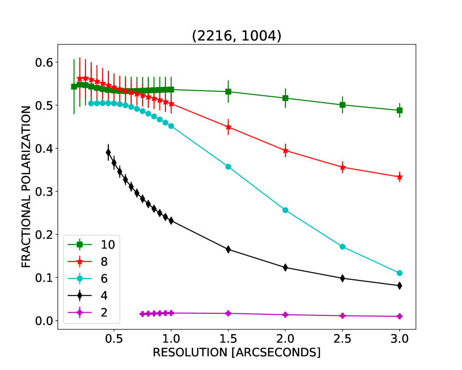
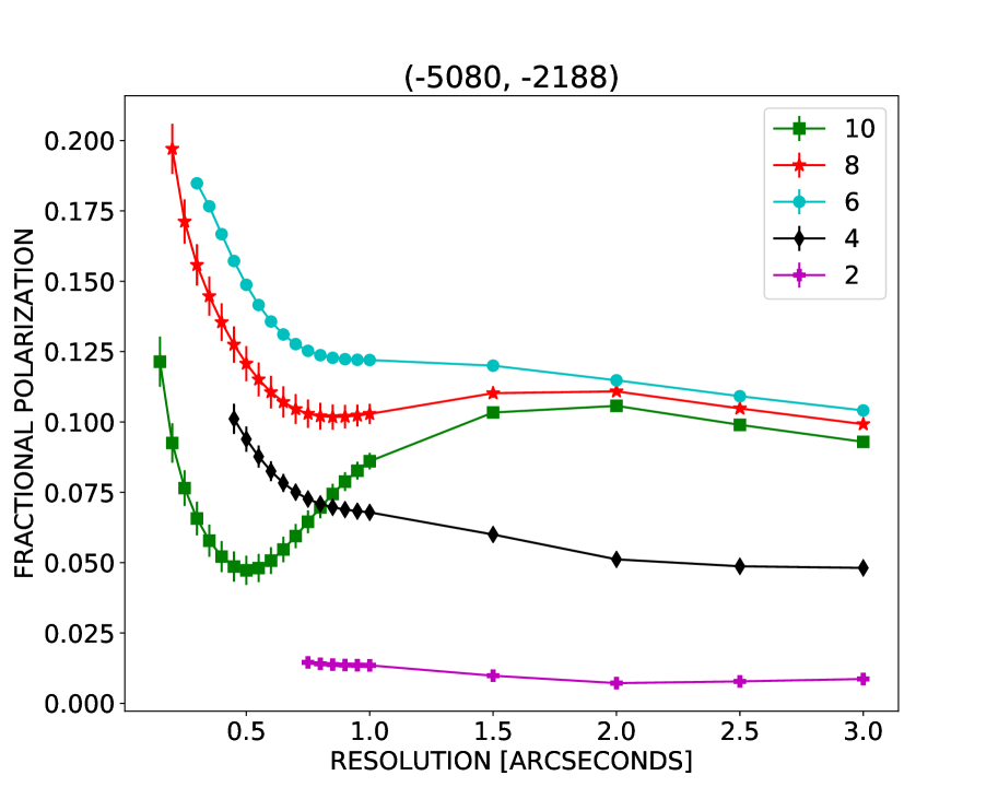
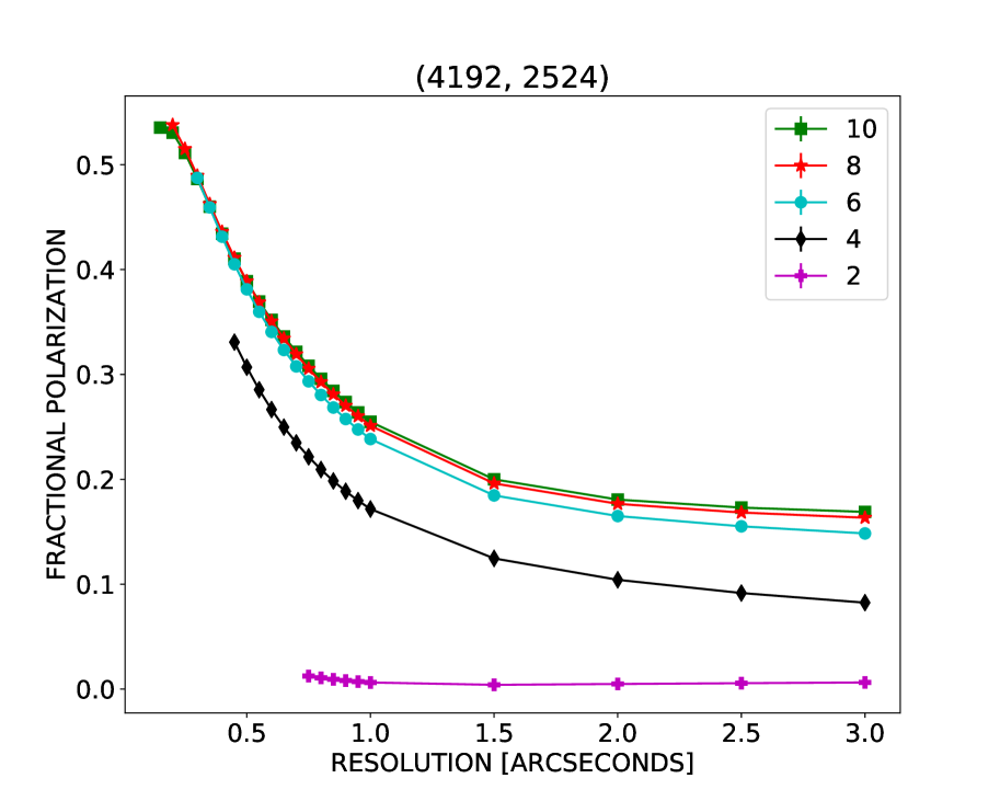
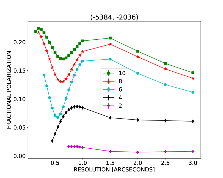
Figure 7: Fractional polarization as a function of resolution. The frequencies shown are: $10$ GHz (green), $8$ GHz (red), $6$ GHz (blue), $4$ GHz (black) and $2$ GHz (purple). The complex behavior, and the lack of a rise in the low-frequency plots, demonstrates considerable beam-related depolarization remains at the highest resolutions available.

5 Modeling the $RM$ Screen at $0.3\arcsec$ Resolution

In the previous section, we showed the result that the depolarization of the majority of the lines of sight are non monotonic, showing fluctuating, and in some cases oscillating, fractional depolarization with increasing wavelength. For all lines of sight, there is strong overall depolarization, resulting in almost complete depolarization by a frequency of $2$ GHz. This strongly suggests ‘beam depolarization’ due to the turbulent medium on scales less than $0.7\arcsec$ is an important contributor to the depolarization.

The higher frequency data provide much higher resolution – at $6$ GHz, the limiting resolution is $0.3\arcsec$. Noting that the oscillatory behavior in the depolarization is restricted to the lower frequencies – it is not seen above $6$ GHz in all the $2000$ independent lines of sight – we can determine the properties of the Faraday screen with the high resolution, high frequency data alone, and use this to predict the lower frequency, lower resolution data which displays the complex depolarization behavior. A good match between such a prediction and the observations would be strong evidence that the foreground screen alone is primarily responsible for the majority of the depolarization. That is, the depolarization is dominantly beam-related.

To test this idea, we fitted simple models incorporating random unresolved fluctuations in a depolarizing screen to our high frequency high resolution data. We used the LMFIT software package to perform a nonlinear least-squares fitting of our data to the following model:

$$p=p_{0}e^{2i\chi_{0}}e^{2iRM\lambda^{2}-2\sigma^{2}\lambda^{4}},$$ (12)

where $RM$ is the Faraday depth due to any large-scale magnetic field, $p_{0}$ and $\chi_{0}$ are the intrinsic ’zero-wavelength’ fractional polarization and polarization angle respectively, and $\sigma$ is the Faraday dispersion due small scale, random, Gaussian fluctuations in Faraday depths within clouds of fixed size (Burn, 1966):

$$\sigma=812n_{t}B_{t}d\sqrt{N}\quad\quad[\mathrm{rad\,m}^{-2}]$$ (13)

where $N=L/d$ is the number of turbulent cells of size $d$ lying along the path length $L$, $n_{t}$ is the electron density in the cell, and $B_{t}$ is the magnetic field of the cell.

Note however that the dispersion parameter can also describe the spread due a linear gradient across a Gaussian beam - the first order term in a Taylor series expansion defined in Eq. 2 of Laing et al. (2008).

We performed fitting without weighting so that we do not disadvantage the high frequency data since they are of low signal-to-noise ratios and are relatively less represented due to frequency averaging. We considered only pixels with an intensity in the $2$ GHz image $5\times$ the off-source noise. Figure 8 shows a few examples of the fitting of this model to the data, indicating a reasonable fit to the data, as judged by eye.

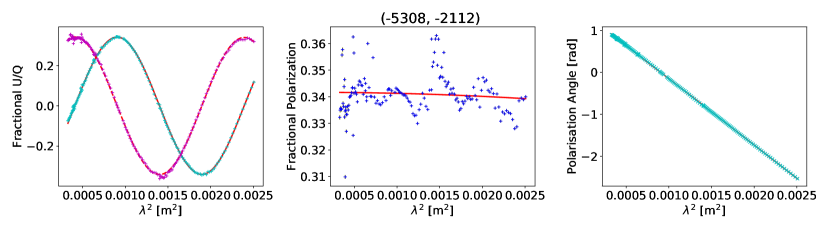
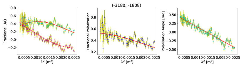
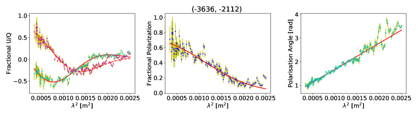
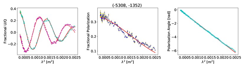
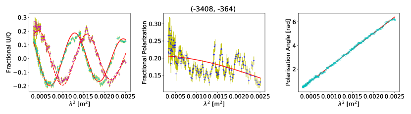
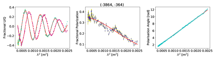
Figure 8: Examples of a simple depolarization screen fitted to the $6-18$ GHz, $0.3\arcsec$ data of Cygnus A. The left column plots show the fractional Stokes $Q/I$ and $U/I$, the middle column shows the fractional polarization and right column shows the polarization angle, all as a function of $\lambda^{2}$. The data are predicted very well by this simple depolarization model.

The modeling returns values of the intrinsic (zero-wavelength) fractional polarization and polarization position angle, the Faraday depth ($\phi$), (here equal to the RM, as there are no significant deviations from $\lambda^{2}$), and the Faraday dispersion, $\sigma$, which describes the overall decline in fractional polarization between 18 and 6 GHz, at $0.3\arcsec$ resolution. Figure 9 shows images of the intrinsic fractional polarization across the two lobes (top row), the rotation measure (middle row), and the Faraday dispersions (bottom row). These are discussed in the next section. The left panels show the eastern lobe, the right hand panels the western lobe. We consider only pixels with $\sigma_{RM}/RM<0.2$ and $\sigma_{p_{0}}/p_{0}<0.2$, where $\sigma_{RM}$ and $\sigma_{p_{0}}$ are errors derived from the fits. This step ensures that we remove pixels which are less reliable.

5.1 Intrinsic Fractional Polarization

The derived intrinsic fractional polarization maps indicate that Cygnus A is highly polarized in nearly all areas, with typical values between 15% and 45%, and some as high as 70%. Even the inner portions of the eastern lobe – which depolarizes the most rapidly – show ’zero-wavelength’ polarizations similar to all other parts of the source. These are consistent with the 10 GHz map shown in Fig. 3. These results indicate that the low polarization seen at intermediate wavelengths are not intrinsic to the source. The low fractional polarization regions across the lobes seen at lower frequencies and resolutions are clearly largely a result of unresolved fluctuations in a magnetized foreground screen.

5.2 Rotation Measure

The rotation measure maps presented here are much more detailed than those derived by Dreher et al. (1987). These new results extend the $RM$ mapping into the inner region of the eastern lobe, and the tail of the western lobe. Both areas reveal extremely high $RM$s, resulting in an increased maximum $RM$ range: $-4500$ and $+6400$ rad m^-2 in the eastern lobe, and $-5000$ and $+3000$ in the western lobe. More striking is that the inner large rotation measures have opposite signs suggesting field reversal in the surrounding material. In most regions the $RM$ gradients are typically a few $100$ rad m^-2 arcsec^-1, with a few regions having gradients as high as $\sim 1000$ $\mathrm{rad\,m}^{-2}\,$arcsec^-1. The $RM$ changes sign on 3–20 kpc scales, and this change in sign seems to occur along the source axis, particularly in the eastern lobe. The $RM$s are relatively smooth across the western lobe, and in general increase with decreasing radial distance from the AGN. These confirm the results, made with more limited data, given by Perley & Carilli (1996). The $RM$s in the eastern lobe are relatively chaotic at this resolution, with the $|RM|$ showing no clear radial dependence but instead occurring in bands of high and low $RM$, similar to those seen in M84, 3C 353, 0206+35, and 3C 270 (Guidetti et al., 2011). Note that, with the exception of the enhanced $RM$ arc surrounding hotspot B found by Carilli et al. (1988), there is no evident correlation between the $RM$ values and the source brightness or with any of the evident structures in total intensity (i.e., the hotspot, jet, or filaments). This supports the interpretation that the observed $RM$ structures originate outside the source of the emission.

5.3 Random $RM$ Fluctuations

The bottom row of Fig. 9 shows the dispersion images from the $0.3\arcsec$ modeling. This parameter essentially describes the rate of depolarization between $18$ and $6$ GHz, as seen in Fig. 8. The error in these measurements is $\leq 10$ $\mathrm{rad\,m}^{-2}\,$for the brighter, outer regions in the lobe, rising to $\leq 50$ $\mathrm{rad\,m}^{-2}\,$at the tails of the lobe.

Typical dispersion values across the western lobe are $\lesssim 300$ $\mathrm{rad\,m}^{-2}\,$with a few regions having dispersions of up to $\sim 400$ $\mathrm{rad\,m}^{-2}\,$. Regions with very small dispersions close to zero may be a result of a lack of significant depolarization, or due to repolarization. The latter can be real or due to the noise – the form of Eq. 12 does not account for this effect. The dispersion values in the eastern lobe are similar to those in the western lobe, with typical $RM$ dispersions of $\lesssim 200$ $\mathrm{rad\,m}^{-2}\,$in the extreme parts of the lobe close to the hotspots, and regions closest to the AGN having dispersions of $\sim 400$ $\mathrm{rad\,m}^{-2}\,$, with a few spatially narrow regions having dispersion of $\sim 800$ $\mathrm{rad\,m}^{-2}\,$. However, these latter regions are associated with very large errors – 100 – 300 $\mathrm{rad\,m}^{-2}\,$, and are mostly coincident with regions of large $RM$ gradients and low polarization, similar to 3C 31; see Appendix C in Laing et al. (2008). The discussion of the actual origin of these narrow filaments will be addressed in paper 2. Note that the dispersions are rather chaotic in the innermost regions of the eastern lobe, likely indicating considerable structure remains on scales less than $0.3\arcsec$. The similarity in $\sigma$ across both lobes is also suggestive of a common medium encompassing both lobes, with the more complex structures in the eastern lobe likely a result of the Laing-Garrington effect (Garrington et al., 1988, 1991; Laing, 1988) – with the eastern lobe further from us than the western lobe. However, it should be noted that this effect cannot not explain the banded $RM$ distribution across the lobes. Instead, the bands indicate the ordering of the large-scale magnetic field component, with a relatively large field ordering across the western lobe.

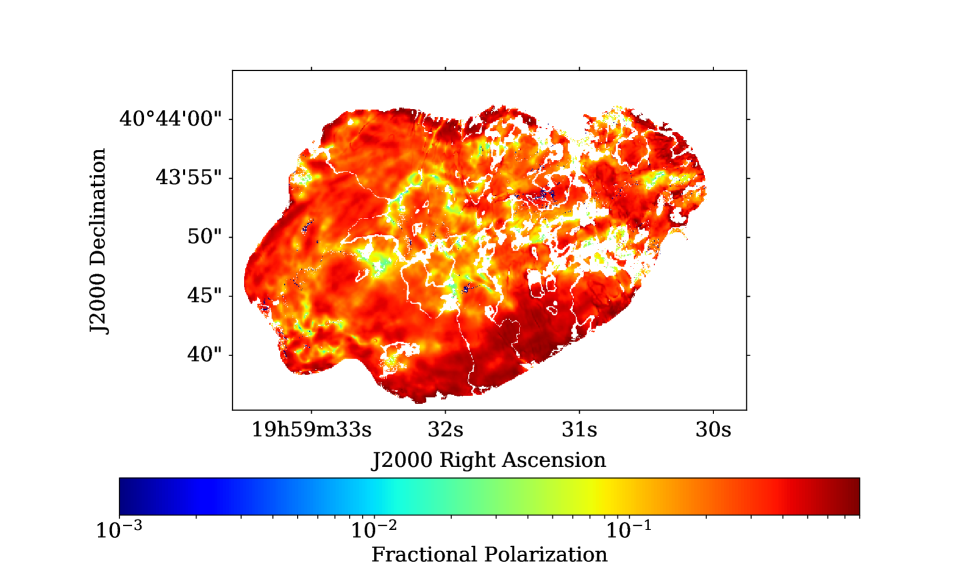
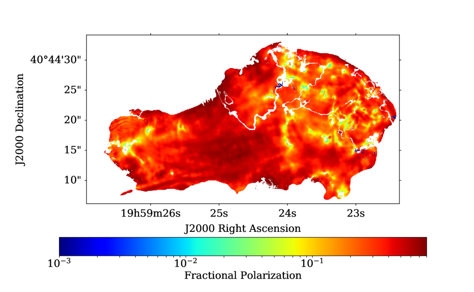
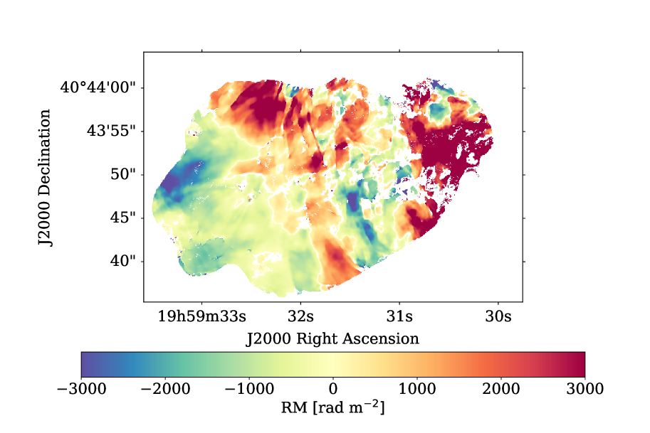
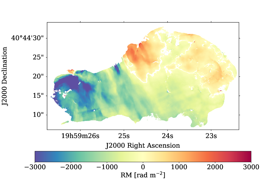
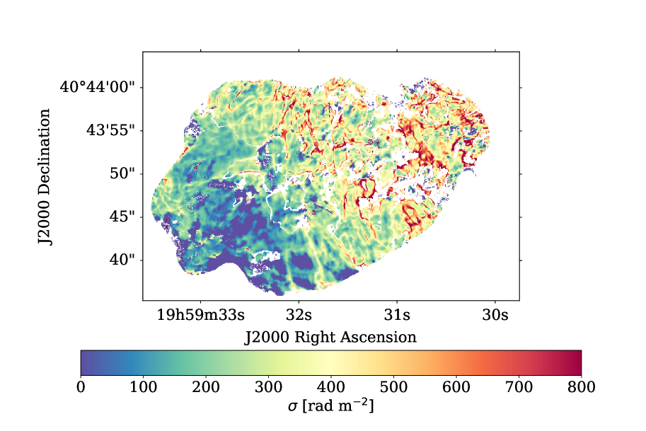
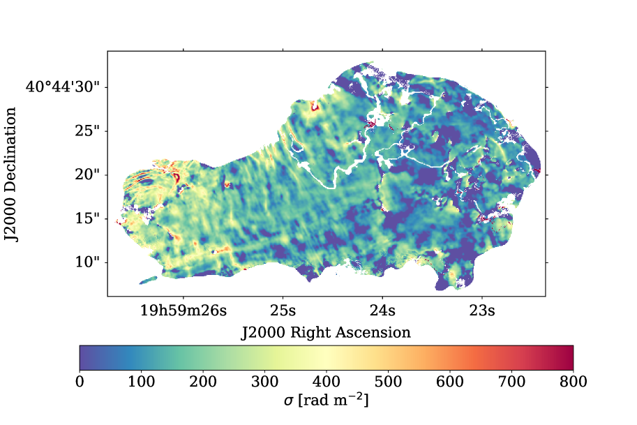
Figure 9: $QU$-fitting parameter maps at $0.30\arcsec$ ($6-18$ GHz). The top row shows the intrinsic fractional polarization, the middle row shows the rotation measures, and the bottom row the $RM$ dispersions. The intrinsic fractional polarization is consistent with the maps at high frequencies and high resolution, see Fig. 3 and 6. Rotation measures range between $-4500$ to $+6400$ $\mathrm{rad\,m}^{-2}\,$in the eastern lobe and $-5000$ and $+3000$ $\mathrm{rad\,m}^{-2}\,$in the western lobe. The RM changes sign on $3-20$ kpc scales, with a banded structure orthogonal to the source axis, particularly evident in the western lobe. The lobes depolarize much more rapidly in the inner regions towards the AGN as seen in the $\sigma$ map. Pixels shown have relative error in $RM$ and $p_{0}$ of less than 0.2.

5.4 Intrinsic Magnetic Field Orientations

The fitting described above determines the intrinsic polarization (‘zero-wavelength’) angle values, from which we can directly determine the intrinsic projected magnetic field ($\chi_{0}+\pi/2$) of the source. Figure 10 shows the magnetic field orientations superposed on a color-coded image of the total intensity at 4 GHz. The fields follow the boundaries and filamentary structures of the lobe emission. This behavior is quite common in radio galaxies, seen for example in 3C 465 (Eilek, & Owen, 2002), Hydra A (Taylor et al., 1990), and Pictor A (Perley et al., 1997), and is generally understood as an effect resulting from shearing (and compression at outer parts of the lobes) of the tangled lobe magnetic field at the lobe boundary, resulting in suppression of field components normal to the lobe boundaries (Laing, 1980). The field vectors are generally smooth across the western lobe and brighter parts of the eastern lobe, while becoming slightly chaotic in the inner region of the eastern lobe. As with the other fitted parameters, this is likely due to significant structures on scales less than the $0.3\arcsec$ resolution utilized here.

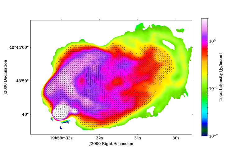
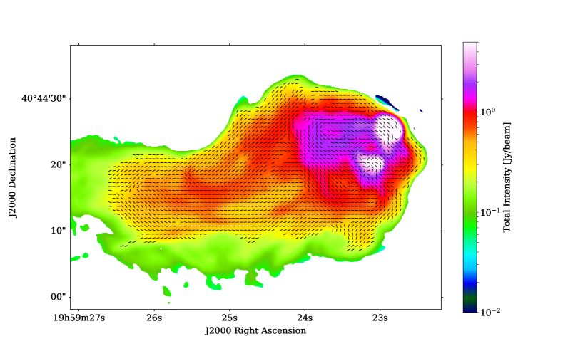
Figure 10: Intrinsic magnetic field orientation at $0.30\arcsec$ resolution across the lobes. These are superimposed on a color image of the total intensity at $3.979$ GHz and $0.54\arcsec\times 0.44\arcsec$ resolution. The field vectors follow the boundaries of the source as well as the filamentary structures.

5.5 $RM$ vs. Random $RM$ Fluctuations

One question that arises is whether the observed $RM$ dispersions are correlated with the rotation measures. This might occur if the major $RM$ structures are associated with a mixing layer surrounding the source. The higher $RM$s might then be associated with higher field values within the turbulent cells. To address this question, we plot in Fig. 11 the $RM$ vs $\sigma$ for lines of sight classified as described in section 4.1. Shown are only those lines of sight with relative errors in $RM$ dispersion less than 80%. There is no clear correlation between these two quantities, from which we conclude that the $RM$ dispersions are not directly a result of the observed $RM$, suggesting that the observed large-scale $RM$ are not coming from a mixed region. However, there is a clear tendency for regions of very high $RM$ to have high dispersions. A likely explanation is that a high $RM$ gradient across the resolution beam will cause a larger apparent depolarization, leading to an apparent increase in the dispersion. The regions of the high gradients are the inner lobes, where the highest $RM$s are accompanied by high dispersions.

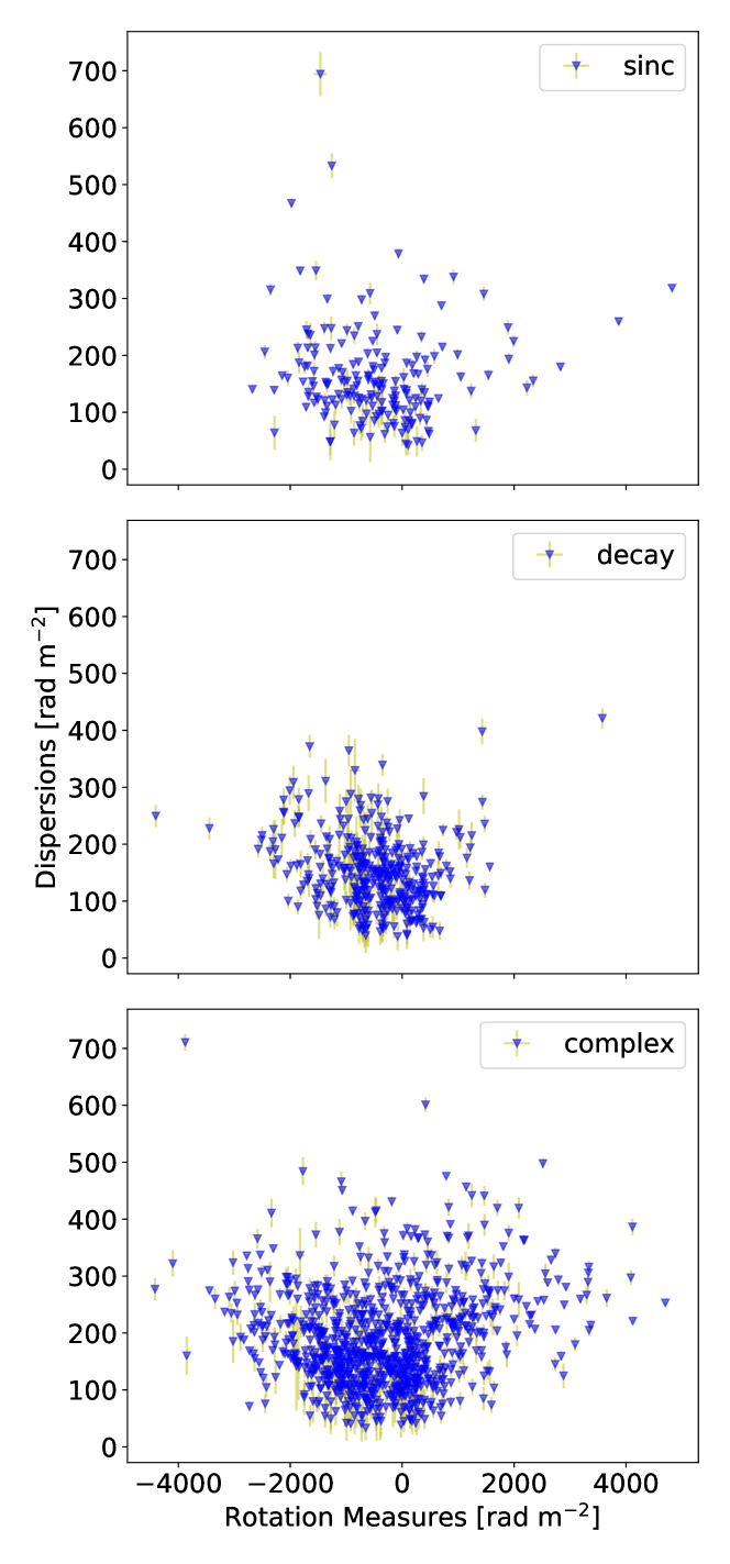
Figure 11: Faraday dispersions, $\sigma$, as a function of rotation measures, $RM$. These are separated based on their classes (see section 4.1): sinc-like, smooth decay and complex decay. There is no clear correlation between the $RM$ and $\sigma$. Suggesting that the observed $RM$s are not directly related to the observed depolarizations (decrease of fractional polarization with increasing $\lambda^{2}$).

5.6 Jet Rotation Measures and Magnetic Field Orientation

To obtain detailed solutions for the jets, we performed the above fitting separately for regions enclosing the jet emission. Figure 12 shows fractional polarization, rotation measure, Faraday dispersion and magnetic field orientation across the western jet. The pixels shown have $\sigma_{RM}/RM<0.2$. No reliable solutions were found on or close to the counter jet – even with RM-synthesis. The analysis of this region (and nearby structures such as the nucleus and the ring structure in the eastern lobe) awaits more sensitive observations at higher frequencies.

The intrinsic field orientations lie parallel to the jet axis across most parts of the jet where the jet polarization is visible. This polarization behavior along the jet is common in strong FR II sources (Bridle, & Perley, 1984). The rotation measures of the jet are very similar to those of the lobe (see Fig. 9) both in magnitude $\sim$ -300 to -2000 rad m^-2, and angular scale $\sim$ 2 - 5 kpc, again supporting the argument that the origin of the $RM$ is exterior to the source. The jet has similar Faraday dispersions as those of the lobe emission in the vicinity of the jet: $\sim$ a few 100 rad m^-2 – with slight (not conclusive) indication of larger dispersions towards the nucleus. The jet is intrinsically highly polarized – with fractional polarizations $\sim$ 20% to 50%.

The similarity of the jet $RM$ to that of the lobes has been used to argue against mixing of external gas into the synchrotron-emitting regions – see Taylor & Perley (1993) in the case of Hydra A.

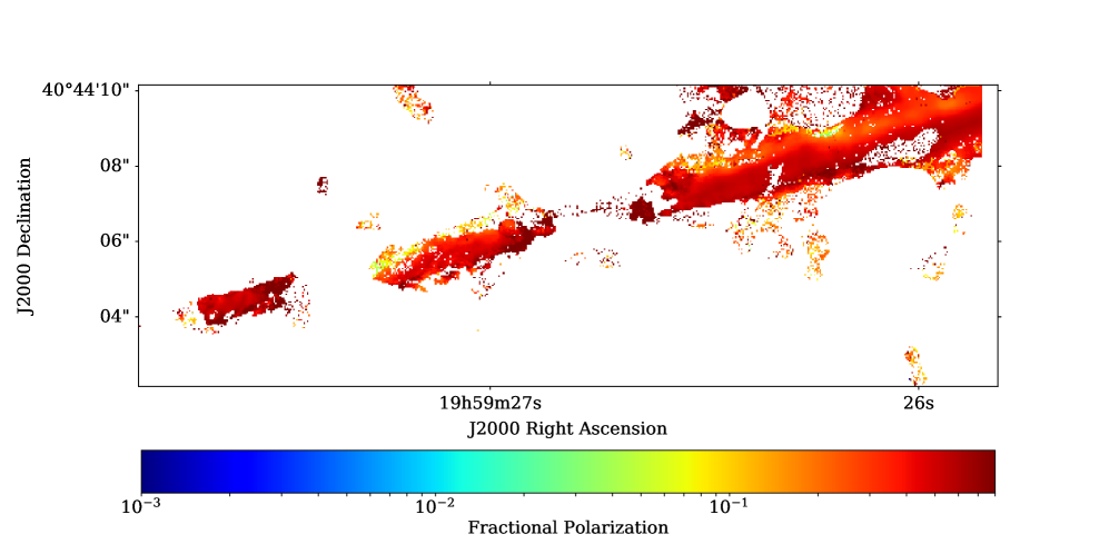
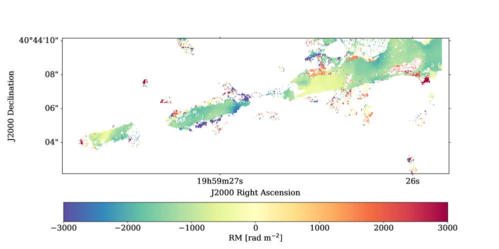
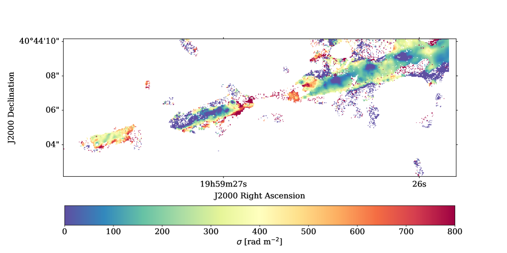
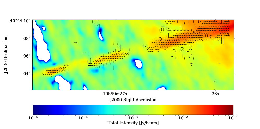
Figure 12: Fitted parameters across the western jet. Top to bottom are the intrinsic fractional polarization, rotation measure, Faraday dispersion and magnetic field vectors along the jet, respectively. The jet is intrinsically highly polarized $\sim$ 20% - 50%. The $RM$s and $\sigma$ within the jet are similar to the $RM$s of the adjacent lobe – indicating a similar origin for both. The field vectors lie parallel to the jet axis.

6 Predicting Low Frequency Depolarization

Section 4.2 showed that beam depolarization – depolarization from transverse fluctuations unresolved by the resolution beam – is an important factor in the depolarization of Cygnus A. Can we state that the observed depolarizations are entirely explained by this effect? This is an important question, which can only be fully answered by observations with much higher resolution – likely better than $0.20\arcsec$ at $2$ GHz – which are not possible with current instruments. However, there is a hint in Fig. 3 and 6, showing the polarization as a function of resolution, and frequency, that a significant fraction of the foreground depolarization is resolved out by a resolution of $0.45\arcsec$, which raises the question of whether the high-resolution, high frequency foreground screen images shown in Fig. 9 can be used to predict the lower-frequency, lower-resolution images where the depolarization effects are very strong. An accurate prediction would be strong evidence for a screen origin of all, or nearly all, the observed depolarization.

We assume that the fractional polarization, $p_{0}$ and polarization angles, $\chi_{0}$, derived in section 5 represent the intrinsic polarization properties of the source. Further, we assume that the rotation measure map is an accurate representation of the foreground Faraday rotating screen on a $0.3\arcsec$ scale – essentially assuming that this resolution has fully resolved the $RM$ screen. With these, we can calculate the low frequency polarization ($<$6 GHz) at $0.3\arcsec$ resolution, by simply rotating the observed polarization angle by $RM\lambda^{2}$ as follows

$$P(\lambda^{2})=p_{0}Ie^{2\text{i}\chi_{0}}e^{2\text{i}RM\lambda^{2}}.$$ (14)

We estimated $I$ at $0.30\arcsec$ across 2-18 GHz first by determining the spectral index at this resolution between 6-18 GHz, and then using this spectral index to extrapolate the total intensity at low frequencies. We then convolved (using AIPS task ’CONVL’) the resulting estimates of the $Q$, $U$ and $I$ to the desired resolution ($0.75\arcsec$) providing the model images. These were then compared to the observed polarizations.

Figure 13 shows a few illustrative examples showing our original data at $0.75\arcsec$ (in black) and the model predictions (in red). The left column shows the fractional polarization as a function of $\lambda^{2}$, the middle column shows the polarization angle as a function of $\lambda^{2}$, and the right column shows the amplitude of the Faraday depths.

Table 3 shows the result of the predictions. The top two rows show examples with smoothly decaying fractional polarization as a function of $\lambda^{2}$. The top row shows an example where the predictions match the data very well – $\sim 13\%$ of the smooth decaying lines of sight fit as well as this. The second row shows an example in which the prediction underestimates the rate of depolarization – denoted in Table 3 as ’approx’. About $\sim 72\%$ of the lines of sight fall within this category. The remaining lines of sight ($\sim 15\%$) are not accurately predicted by our simple model (denoted in Table 3 as ’N/A’).

The bottom four rows show examples of lines of sight with oscillatory behavior. In general, the presence of an oscillatory depolarization is well predicted by our model. This result suggests that although the dominant depolarization mechanism is associated with unresolved fluctuations, there must be present in these cases larger-scale components responsible for the oscillatory depolarization characteristics, likely operating on scales only a little less than our standard $0.75\arcsec$ resolution.

The extraordinarily good fit shown in the third row is not common, however, and in general, the predicted nulls occur at longer $\lambda^{2}$ values than the data, so that the predicted peaks in the Faraday spectrum are too close together, as can be seen in the second column. See results of the predictions for sinc-like lines of sight in first row, column 12 to 14. Results for complex lines of sight are given in row 3 to 5 and same columns.

Thus, overall, on average (weighted by the total number of lines of sight in each class) we find that $\sim 14\%$ of the lines of sight are accurately predicted (within measurement errors), and $\sim 72\%$ have the correct functional form, but with a scaling error, and $\sim 14\%$ of the predictions are incorrect.

What could be causing the shifting of the predicted nulls to higher $\lambda^{2}$ as well as underestimating the depolarizations? The simplest explanation for the latter is that the $0.3\arcsec$ resolution image from which these estimates are made is missing some smaller-scale structure. This is a reasonable conclusion given that we are still seeing depolarizations at $0.30\arcsec$ which we characterized using $\sigma$. The shifting of the nulls to higher $\lambda^{2}$, on the other hand, is caused by an underestimation of the $RM$ difference between the ‘patches’ of polarized emission as resolved on the $0.3\arcsec$ $RM$ image. It is not clear to us why this small underestimation occurs.

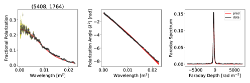
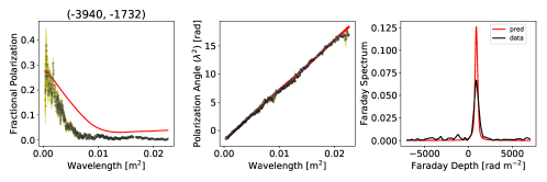
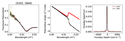
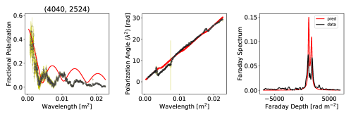
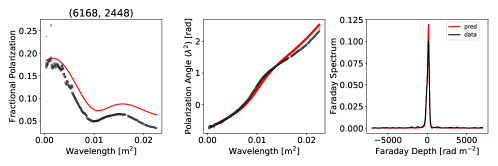
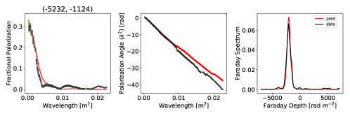
Figure 13: Model predictions of low resolution, $0.75\arcsec$, data using the high resolution, high frequency data. The left column shows the fractional polarization, the middle column the polarization position angle, and the right column the Faraday spectra. Black shows the original data, and red shows the predictions. The simple model fits the data remarkably well for about 2/3 of the LoS.

7 Summary

In this paper we have presented the results from our wideband ($2-18$ GHz), high spectral resolution polarimetry data on Cygnus A. We have shown how the fractional polarization varies as a function of frequency and resolution. We also conducted a Faraday rotation analysis using high frequency data, $>6$ GHz at $0.30\arcsec$ resolution. In this Faraday rotation study, we derived maps of rotation measures ($RM$), intrinsic fractional polarization ($p_{0}$), intrinsic polarization angles ($\chi_{0}$), and $RM$ dispersions ($\sigma$), from which we predict the depolarization behavior at lower frequencies and resolutions, with remarkable success. A complete analysis (physical interpretation) of our full band data will be presented in paper 2. The data are to be made publicly available immediately once our second paper – the analysis paper– gets accepted.

A summary of our results shows:

1. All lines of sight through the lobes depolarize significantly with decreasing frequency. There is no relation between depolarization behavior and the various structural features (hot spots, filaments, jet, etc.). The eastern lobe, particularly those regions nearer the nucleus, depolarize at higher frequencies than the western lobe.

2. The distribution of the fractional polarization across the lobes is smooth at high frequencies, but becomes increasingly clumpy on $\sim 1$ kpc scales, at low frequencies.

3. The fractional polarization as a function of $\lambda^{2}$ for the different lines of sight reveal complex depolarization behaviors: some lines of sight smoothly depolarize, while others show oscillations, which in extreme cases have ‘sinc-like’ behavior. By classifying these polarization behaviors into three simple categories: i) smooth decaying, i) sinc-like, and iii) complex, we find that $25\%$ fall into the first class, $11\%$ the second and $50\%$ are complex. There is a tendency for more complex decay in the eastern lobes, with relatively fewer smooth decay and sinc-like behaviors. The distribution across the the western lobe, on the other hand, consists mostly of smooth decay, particularly at the extremes of the lobes, and complex behavior. There is no clear spatial correlation between these decay patterns across the lobes, except that they are not random but are clumped on few-kpc scales.

4. Lines of sight with oscillations in their depolarization behavior also show strong deviations of the polarization angle from linearity.

5. The lobe emission also depolarizes significantly with decreasing resolution. The inner region of the eastern lobe (closest to the AGN), depolarizes more rapidly than other regions of this lobe.

6. Plots of fractional polarization as a function of resolution and frequency for different lines of sight reveal that the beam-related effects are complicated, and that our observations do not have sufficient resolution to completely resolve the depolarizing structures present in or around Cygnus at frequencies below $6$ GHz.

7. The $RM$ values derived are consistent with those found by Dreher et al. (1987); Perley & Carilli (1996), and extend those results to the weaker emission nearer the nucleus. Our new observations reveal very high $RM$ values at the tails of the lobes – ranging between $-4500$ and $+6400$ $\mathrm{rad\,m}^{-2}\,$in the eastern lobe, and $-5000$ and $+3000$ $\mathrm{rad\,m}^{-2}\,$in the western lobe. We find that the $RM$ values in the eastern lobe occurs in bands of low and high $RM$ along the source-axis. The $RM$ values are ordered on $3-20$ kpc scales. There is no relation between the RM values and the presence of structural features in the total intensity (hotspots, jet, filaments, etc.).

8. The intrinsic magnetic fields of the source follow the boundary and filamentary structures of the lobes – consistent with other radio galaxies. The only exception is the inner region of the eastern lobe where the fields appear to be slightly chaotic.

9. The derived intrinsic fractional polarization of the source found from analysis of the high frequency data alone at $0.3\arcsec$ resolution shows that Cygnus A is intrinsically highly polarized, with typical fractional polarizations between 15% to 45%, and some regions as high as $70\%$. The intrinsic fractional polarization of the inner region of the eastern lobe is very similar to that of the rest of the lobe, indicating that this region is not intrinsically unique, and that the observed depolarizations, and rapid depolarizations have an external origin.

10. We find that the $RM$ dispersions across both lobes decrease with increasing distance from the nucleus. The outermost regions in both lobes have small RM dispersions $\sim 0$ rad m^-2. These increase towards the nucleus to typical values of $\sim 200$ $\mathrm{rad\,m}^{-2}\,$to $400$ $\mathrm{rad\,m}^{-2}\,$. The innermost regions of the eastern lobe show the highest dispersions – up to $\sim 800$ $\mathrm{rad\,m}^{-2}\,$. The $RM$ dispersions are weakly correlated with the observed $RM$, again suggesting that the $RM$ are external to the lobes.

11. Assuming that the derived $p_{0}$, $\chi_{0}$, and $RM$ generated from the high frequency, high resolution data represent the intrinsic polarization properties of the source, and that there is no synchrotron emission in the external medium, we generated predictions of the low frequency polarization emission at $0.3\arcsec$ resolution, which were then convolved to our resolution of $0.75\arcsec$. Comparison of the predictions with the observations show remarkable agreement, with about $14\%$ of the lines of sight predicted accurately, and a further $72\%$ with the correct shape, but with small scale errors. This result supports the interpretation that the majority of the observed depolarization is due to unresolved fluctuations, on the $0.3$ – $0.7$ arcsecond scale, in the external medium.

8 acknowledgments

Support for this work was provided in part by the National Aeronautics and Space Administration through Chandra Award Number GO5-16117B issued by the Chandra X-ray Center, which is operated by the Smithsonian Astrophysical Observatory for and on behalf of the National Aeronautics Space Administration under contract NAS8-03060. The financial assistance of the South African Radio Astronomy Observatory (SARAO) towards this research is hereby acknowledged (www.ska.ac.za). Additional financial assistance of the National Radio Astronomy Observatory (NRAO) a facility of the National Science Foundation operated under cooperative agreement by Associated Universities, Inc is acknowledged. This work is based upon research supported by the South African Research Chairs Initiative of the Department of Science and Technology and National Research Foundation. We thank Larry Rudnick for his enthusiastic assistance in the interpretation of complex polarimetric data. We also thank the reviewer for providing insightful suggestions for improving our findings.

References

- Alexander et al. (1984) Alexander, P., Brown, M. T., & Scott, P. F. 1984, MNRAS, 209, 851
- Brentjens & de Bruyn (2005) Brentjens, M. A., & de Bruyn, A. G. 2005, A&A, 441, 1217
- Bridle, & Perley (1984) Bridle, A. H. & Perley, R. A. 1984, ARA&A, 22, 319
- Burn (1966) Burn, B. J. 1966, MNRAS, 133, 67
- Carilli et al. (1988) Carilli, C. L., Perley, R. A., & Dreher, J. H. 1988, ApJ, 334, L73
- Carilli et al. (1989) Carilli, C. L., Dreher, J. W., & Perley, R. A. 1989, Hot Spots in Extragalactic Radio Sources, 51
- Carilli et al. (1994) Carilli, C. L., Bartel, N., & Diamond, P. 1994, AJ, 108, 64
- Clegg et al. (1992) Clegg, A. W., Cordes, J. M., Simonetti, J. M., et al. 1992, ApJ, 386, 143
- Cornwell & Wilkinson (1981) Cornwell, T. J., & Wilkinson, P. N. 1981, MNRAS, 196, 1067
- Cornwell (2008) Cornwell, T. J. 2008, IEEE Journal of Selected Topics in Signal Processing, 2, 793
- de Vries et al. (2018) de Vries, M. N., Wise, M. W., Huppenkothen, D., et al. 2018, MNRAS, 478, 4010
- Dreher (1979) Dreher, J. W. 1979, ApJ, 230, 687
- Dreher et al. (1987) Dreher, J. W., Carilli, C. L., & Perley, R. A. 1987, ApJ, 316, 611
- Duffy et al. (2018) Duffy, R. T., Worrall, D. M., Birkinshaw, M., et al. 2018, MNRAS, 476, 4848
- Eilek, & Owen (2002) Eilek, J. A., & Owen, F. N. 2002, ApJ, 567, 202
- Fabbiano et al. (1979) Fabbiano, G., Doxsey, R. E., Johnston, M., Schwartz, D. A., & Schwarz, J. 1979, ApJ, 230, L67
- Fanaroff & Riley (1974) Fanaroff, B. L., & Riley, J. M. 1974, MNRAS, 167, 31P
- Garrington et al. (1988) Garrington, S. T., Leahy, J. P., Conway, R. G., et al. 1988, Nature, 331, 147
- Garrington et al. (1991) Garrington, S. T., Conway, R. G., & Leahy, J. P. 1991, MNRAS, 250, 171
- Giacconi et al. (1972) Giacconi, R., Murray, S., Gursky, H., et al. 1972, ApJ, 178, 281
- Greisen (2003) Greisen, E. W. 2003, Information Handling in Astronomy - Historical Vistas, 109
- Greisen et al. (2009) Greisen, E. W., Spekkens, K., & van Moorsel, G. A. 2009, AJ, 137, 4718
- Guidetti et al. (2011) Guidetti, D., Laing, R. A., Bridle, A. H., et al. 2011, MNRAS, 413, 2525
- Halbesma et al. (2019) Halbesma, T. L. R., Donnert, J. M. F., de Vries, M. N., et al. 2019, MNRAS, 483, 3851
- Heald (2009) Heald, G. 2009, Cosmic Magnetic Fields: From Planets, to Stars and Galaxies, 591
- Hinshaw et al. (2013) Hinshaw, G., Larson, D., Komatsu, E., et al. 2013, ApJS, 208, 19
- Killeen et al. (1986) Killeen, N. E. B., Bicknell, G. V., & Ekers, R. D. 1986, ApJ, 302, 306
- Laing (1980) Laing, R. A. 1980, MNRAS, 193, 439
- Laing (1988) Laing, R. A. 1988, Nature, 331, 149
- Laing et al. (2008) Laing, R. A., Bridle, A. H., Parma, P., et al. 2008, MNRAS, 391, 521
- Mitton (1971) Mitton, S. 1971, MNRAS, 153, 133
- Perley et al. (1984) Perley, R. A., Dreher, J. W., & Cowan, J. J. 1984, ApJ, 285, L35.
- Perley & Carilli (1996) Perley, R. A., & Carilli, C. L. 1996, Cygnus A – Studay of a Radio Galaxy, 168.
- Perley et al. (1997) Perley, R. A., Roser, H.-J., & Meisenheimer, K. 1997, A&A, 328, 12
- Perley et al. (2001) Perley, R.A., Chandler, C.J., Butler, B.J., and Wrobel, J.M. 2001 ApJ, Lett, 739:L1
- Perley, & Butler (2017) Perley, R. A., & Butler, B. J. 2017, ApJS, 230, 7
- Schnitzeler et al. (2009) Schnitzeler, D. H. F. M., Katgert, P., & de Bruyn, A. G. 2009, A&A, 494, 611
- Simard-Normandin et al. (1981) Simard-Normandin, M., Kronberg, P. P., & Button, S. 1981, ApJS, 45, 97
- Slysh (1966) Slysh, V. I. 1966, Soviet Ast., 9, 533
- Smith et al. (2002) Smith, A. D., Wilson, A. S., Arnaud, K. A., et al. 2002, ApJ, 565, 195
- Snios et al. (2018) Snios, B., Nulsen, P. E. J., Wise, M. W., et al. 2018, ApJ, 855, 71
- Sokoloff et al. (1998) Sokoloff, D. D., Bykov, A. A., Shukurov, A., et al. 1998, MNRAS, 299, 189
- Spinrad & Stauffer (1982) Spinrad, H., & Stauffer, J. R. 1982, MNRAS, 200, 153
- Stockton & Ridgway (1996) Stockton, A., & Ridgway, S. 1996, Cygnus A – Studay of a Radio Galaxy, 1
- Taylor et al. (1990) Taylor, G. B., Perley, R. A., Inoue, M., et al. 1990, ApJ, 360, 41
- Taylor & Perley (1993) Taylor, G. B., & Perley, R. A. 1993, ApJ, 416, 554