Development of a general-purpose machine-learning interatomic potential for aluminum by the physically-informed neural network method

Abstract

Interatomic potentials constitute the key component of large-scale atomistic simulations of materials. The recently proposed physically-informed neural network (PINN) method combines a high-dimensional regression implemented by an artificial neural network with a physics-based bond-order interatomic potential applicable to both metals and nonmetals. In this paper, we present a modified version of the PINN method that accelerates the potential training process and further improves the transferability of PINN potentials to unknown atomic environments. As an application, a modified PINN potential for Al has been developed by training on a large database of electronic structure calculations. The potential reproduces the reference first-principles energies within 2.6 meV per atom and accurately predicts a wide spectrum of physical properties of Al. Such properties include, but are not limited to, lattice dynamics, thermal expansion, energies of point and extended defects, the melting temperature, the structure and dynamic properties of liquid Al, the surface tensions of the liquid surface and the solid-liquid interface, and the nucleation and growth of a grain boundary crack. Computational efficiency of PINN potentials is also discussed.

I Introduction

Large-scale molecular dynamics (MD) and Monte Carlo (MC) simulations constitute an essential component of the multiscale approach in materials modeling and computational design. The most critical ingredient of such simulations is the classical interatomic potentials, whose role is to make computationally fast predictions of the system energy and atomic forces. It is not an exaggeration to say that the results of atomistic simulations are as accurate and reliable as the utilized interatomic potentials. Several forms of interatomic potentials have been developed for different classes of materials. Some of the most popular types of potentials include the embedded-atom method (EAM) potentials (Daw84, ; Daw83, ; Mishin.HMM, ), the modified embedded-atom method (MEAM) potentials (Baskes87, ), the angular-dependent potentials (Mishin05a, ), the charge-optimized many-body potentials (Liang:2012aa, ), the reactive bond-order potentials (Brenner90, ; Brenner00, ; Stuart:2000aa, ), and the reactive force fields (van-Duin:2001aa, ) – to name a few. During the past decade, a new class of machine-learning (ML) potentials has emerged, which is based on a radically different philosophy than the traditional potentials.

The traditional interatomic potentials partition the total energy $E$ into energies $E_{i}$ assigned to individual atoms $i$: $E=\sum_{i}E_{i}$. Each atomic energy $E_{i}$ is expressed as a function of atomic positions $(\mathbf{r}_{i1},\mathbf{r}_{i2},...,\mathbf{r}_{in})$ in the vicinity of atom $i$. This function depends on a small number of fitting parameters $\mathbf{p}=(p_{1},...,p_{m})$, which are optimized on a database composed of experimental data and a relatively small set of energies and/or forces obtained by electronic structure calculations. Once optimized, the potential parameters are fixed once and for all and used for all atomic environments that might be encountered during the subsequent MD and/or MC simulations. Traditional potentials are computationally fast and scale linearly with the number of atoms. As such, they provide access to systems containing millions of atoms and enable MD simulations for tens or even hundreds of nanoseconds. Because they are based on a small number of parameters, the accuracy of traditional potentials is generally not very high. However, the functional form of traditional potentials is motivated by physical understanding of the interatomic bonding in the material in question. As a result, the potentials often demonstrate reasonable transferability to atomic configurations that were not included in the fitting database. Although the energies and forces predicted outside the fitting domain may not be very accurate, they retain some degree of physical sense. Another feature of the traditional potentials is that they are typically general-purpose type. Once released to the community, a potential is used not only for the purpose for which it was intended but for almost any type of simulations that the user might wish to perform.

The emerging class of ML potentials takes a different approach. The physics of interatomic bonding is not considered. The local environment of an atom is mapped directly onto the potential energy surface (PES) using one of the high-dimensional nonlinear regression methods, such as the Gaussian process regression (Payne.HMM, ; Bartok:2010aa, ; Bartok:2013aa, ; Li:2015aa, ; Glielmo:2017aa, ; Bartok_2018, ; Deringer:2018aa, ), the kernel ridge regression (Botu:2015bb, ; Botu:2015aa, ; Mueller:2016aa, ), or an artificial neural network (NN) (Behler07, ; Bholoa:2007aa, ; Behler:2008aa, ; Sanville08, ; Eshet2010, ; Handley:2010aa, ; Behler:2011aa, ; Behler:2011ab, ; Sosso2012, ; Behler:2015aa, ; Behler:2016aa, ; Schutt:148aa, ; Imbalzano:2018aa, ). Other types of ML potentials include the spectral neighbor analysis (SNAP) (Thompson:2015aa, ; Chen:2017ab, ; Li:2018aa, ) and moment tensor (MTP) (Shapeev:2016aa, ) potentials. In most cases, the total energy is again partitioned into atomic contributions. However, instead of position vectors $(\mathbf{r}_{i1},\mathbf{r}_{i2},...,\mathbf{r}_{in})$ of neighboring atoms, a set of local structural parameters $(G_{i}^{1},G_{i}^{2},...,G_{i}^{K})$ is introduced, which encodes the local environment of the atom and is invariant under rotations and translations of the coordinate axes. The approach based on local descriptors was pioneered by Behler and Parrinello (Behler07, ) (who called $G_{i}^{j}$ the symmetry parameters (Behler07, ; Behler:2011ab, )) in the context of NN potentials. Since the size $K$ of the feature vector $(G_{i}^{1},G_{i}^{2},...,G_{i}^{K})$ is fixed, a single NN can be trained for all atoms of the system. The NN (or any other regression model) contains a large number of parameters ($\approx 10^{3}$), which are trained on a large database of first-principles energies and/or forces (typically, for $\approx 10^{3}$ to $\approx 10^{4}$ supercells). A high accuracy of fitting can be achieved, usually on the meV per atom level. The required reference data can be generated by high-throughput density functional theory (DFT) calculations.

The method has a wide scope of applications since the regression and its training do not depend of the nature of chemical bonding in the material. However, the high accuracy and flexibility come at a price: the ML potentials suffer from poor transferability to atomic configurations lying outside the training domain. Since the structure-energy mapping is not guided by any physics or chemistry, the regression only ensures accurate numerical interpolation between the DFT points. Extrapolation outside the domain of known environments is purely mathematical and thus cannot be expected to make physically meaningful predictions. The lack of physics-based transferability presents a challenge to the development of general-purpose type ML potentials.

The recently proposed physically-informed neural network (PINN) model (PINN-1, ) aims to improve the transferability of ML potentials by integrating a NN regression with a physics-based interatomic potential. Whereas the parameters of a traditional potential are permanently fixed, the PINN model predicts the best set of potential parameters for every atomic environment that may be encountered during simulations. To achieve this, the local structural descriptors $(G_{i}^{1},G_{i}^{2},...,G_{i}^{K})$ are fed into a pre-trained NN, which outputs an optimized set of potential parameters $\mathbf{p}_{i}=(p_{i1},...,p_{im})$ for the given atom $i$. These parameters are then used to compute the atomic energy $E_{i}$ with the potential. The atomic energies are summed up to obtain the total energy of the system. Like the mathematical ML potentials mentioned above, the PINN model predicts the PES of the system, from which analytical forces acting on the atoms can be obtained by differentiation. In other words, the PINN model relies on a physics-based interatomic potential, but the potential parameters are adjusted on the fly by a NN according to local environments of atoms. Improved transferability to new environments is expected because extrapolation is now guided by physical insights embedded in the interatomic potential rather than a purely numerical algorithm.

In the previous paper (PINN-1, ), a PINN potential for aluminum (Al) was constructed as a proof of principle. The goal of the present paper is to report on further developments of the PINN method and to construct and test a new, significantly improved version of the general-purpose PINN Al potential.

In Section II, we briefly review the PINN model and describe its modifications in both the core formalism and the training/validation procedures. In Section III, we present the new Al potential with a superior quality over the previous version (PINN-1, ). We test the potential for a wide spectrum of physical properties, such as lattice dynamics, thermal expansion, defect structures and energies in the face-centered-cubic (FCC) Al, and equations of state of several alternate crystalline phases of Al. Next, we apply the potential to compute several properties that require extrapolation to diverse environments and can only be obtained by large-scale simulations (Section IV). The applications include structural and dynamic properties of liquid Al, the melting temperature of Al, as well as the surface tensions of the liquid surface and the solid-liquid interface. Another application involving almost half a million atoms is the growth of a crack on a planar grain boundary. While performing these tests, we evaluate the computational efficiency of the PINN simulations – an important topic that we discuss in Section V. In Section VI, we summarize this work.

II Methodology

II.1 The bond-order potential

The key ingredients of the PINN model are a physics-based interatomic potential, local structural parameters (descriptors), and an artificial NN connecting the descriptors and the potential parameters. We will start by discussing the interatomic potential.

As in (PINN-1, ), we choose an analytical bond-order potential (BOP) (Oloriegbe_PhD:2008aa, ; Gillespie:2007vl, ; Drautz07a, ) capable of describing chemical bonding in both covalent and metallic materials. For a single-component system, the total energy $E=\sum_{i}E_{i}$ is the sum of the atomic energies

$$E_{i}=\dfrac{1}{2}\sum_{j\neq i}\left[e^{A_{i}-\alpha_{i}r_{ij}}-S_{ij}b_{ij}e^{B_{i}-\beta_{i}r_{ij}}\right]f_{c}(r_{ij},d,r_{c})+E_{i}^{(p)},$$ (1)

where $A_{i}$, $B_{i}$, $\alpha_{i}$, $\beta_{i}$, $d$ and $r_{c}$ are parameters. The summation runs over neighbors $j$ of atom $i$. $r_{ij}$ is the distance between the two atoms. The interactions are truncated at a distance $r_{c}$ using the cutoff function

$$f_{c}(r,r_{c},d)=\begin{cases}\dfrac{(r-r_{c})^{4}}{d^{4}+(r-r_{c})^{4}}\enskip&r\leq r_{c}\\ 0,\enskip&r\geq r_{c},\end{cases}$$ (2)

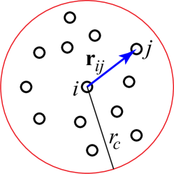
(b)

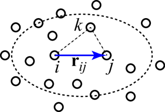
(c)

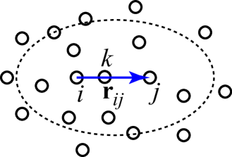
Figure 1: (a) Neighbors $j$ and an atom $i$ within the cutoff sphere of radius $r_{c}$. (b) Atomic bond $i$-$j$ is partially screened by surrounding atoms $k$. The surfaces of constant screening factor are ellipsoids whose poles coincide with the atomic positions $i$ and $j$. (c) If an atom $k$ is located on the bond $i$-$j$, then the screening factor is close to zero and the bond is broken.

where the parameter $d$ controls the truncation smoothness. The cutoff sphere encompasses several coordination shells and typically contains a few dozen atoms (Fig. 1a).

In Eq.(1), the first term in the square brackets describes the repulsion between neighboring atoms at short separations, whereas the second term describes the chemical bonding. The coefficient

$$b_{ij}=(1+z_{ij})^{-1/2},$$ (3)

captures the bond-order effect. Here $z_{ij}$ represents the number of bonds $ik$ formed by the atom $i$ (not counting the bond $i$-$j$, which is included by adding the unity). The bonds are counted with weights that depend on the angle $\theta_{ijk}$ between the bonds $ij$ and $ik$:

$$z_{ij}=\sum_{k\neq i,j}a_{i}S_{ik}\left(\cos\theta_{ijk}-h_{i}\right)^{2}f_{c}(r_{ik},d,r_{c}),$$ (4)

where $a_{i}$ and $h_{i}$ are parameters. The angular dependence is introduced to capture the directional character of covalent bonds. According to Eq.(3), atoms surrounded by a larger number of neighbors have a lower energy per bond (the bond order effect).

All chemical bonds are screened by the screening factor $S_{ij}$ defined by

$$S_{ij}=\prod_{k\neq i,j}S_{ijk},$$ (5)

where the partial screening factors $S_{ijk}$ represent the contributions of individual atoms $k$ to the screening of the bond $i$-$j$. The partial screening factors have the form

$$S_{ijk}=1-f_{c}(r_{ik}+r_{jk}-r_{ij},d,r_{c})e^{-\lambda_{i}(r_{ik}+r_{jk}-r_{ij})},$$ (6)

where $\lambda_{i}$ is the screening parameter (inverse of the screening length). Eq.(6) shows that $S_{ijk}$ has a constant value on a spheroid whose poles coincide with atoms $i$ and $j$ (Fig. 1b). The cutoff spheroid is defined by the condition $r_{ik}+r_{jk}-r_{ij}=r_{c}$ and encompasses all atoms $k$ that contribute to the screening. For atoms $k$ located outside the cutoff spheroid $S_{ijk}=1$ (no contribution to the screening), while for atoms inside cutoff spheroid $S_{ijk}<1$. The closer the atom $k$ to the bond $i$-$j$, the smaller is $S_{ijk}$ and the larger is its contribution to the screening. If one of the atoms $k$ is located on the bond $i$-$j$ (Fig. 1c), then $r_{ik}+r_{jk}-r_{ij}=0$ and $S_{ijk}=1-f_{c}(0,d,r_{c})\ll 1$. Thus, the bond $i$-$j$ is almost completely screened and can be considered as broken. The deviation from complete screening ($S_{ijk}=0$) is controlled by the parameter $d$ in Eq.(2) and avoids division by zero in the analytical differentiation of the potential.

It should be noted that the major semi-axis of the cutoff spheroid has the length $1.5r_{c}$, i.e., is larger than the radius $r_{c}$ of the cutoff sphere. Thus, some atoms lying outside the cutoff sphere can still affect the atomic energy $E_{i}$ indirectly through the screening effect.

The last term in Eq.(1) is an on-site energy given by

$$E_{i}^{(p)}=-\sigma_{i}\left({\displaystyle\sum_{j\neq i}S_{ij}b_{ij}}f_{c}(r_{ij})\right)^{1/2},$$ (7)

$\sigma_{i}$ being a parameter. For covalent materials, $E_{i}^{(p)}$ is added to account for the promotion energy required to change the electronic structure of free atoms when they form covalent bonds. For metallic materials, $E_{i}^{(p)}$ represents the energy of embedding the atom into the local electron density. Indeed, $E_{i}^{(p)}$ can be recast in the form

$$F(\bar{\rho}_{i})=-\sigma_{i}\left(\bar{\rho}_{i}\right)^{1/2},$$ (8)

where

$$\bar{\rho}_{i}=\sum_{j\neq i}S_{ij}b_{ij}f_{c}(r_{ij})$$ (9)

has the meaning of the host electron density on atom $i$. This term is similar to the embedding energy $F(\overline{\rho})$ appearing in the EAM method widely used for metallic systems.

Thus, the BOP potential underlying the PINN model reflects the nature of chemical bonding in both covalent and metallic materials. As such, it can be employed for the modeling of mixed-bonding materials and multi-phase systems containing metal-nonmetal interfaces.

The BOP potential depends on 10 parameters. Eight of them, namely, $A_{i}$, $B_{i}$, $\alpha_{i}$, $\beta_{i}$, $a_{i}$, $h_{i}$, $\sigma_{i}$ and $\lambda_{i}$ are adjusted according to the local atomic environments. The cutoff parameters $r_{c}$ and $d$ are treated as global: once adjusted, they remain the same for all atoms.

II.2 The local structural parameters

The local environment of an atom $i$ is encoded in the rotationally-invariant structural parameters

$$g_{i}^{(l)}(r_{0},\sigma)=\sum_{j\neq i,k\neq i}P_{l}\left(\cos\theta_{ijk}\right)f(r_{ij},r_{0},\sigma)f(r_{ik},r_{0},\sigma),\enskip\enskip l=0,1,2,...,l_{max},$$ (10)

where $P_{l}(x)$ are Legendre polynomials of order $l$. The radial function is the Gaussian

$$f(r,r_{0},\sigma)=\dfrac{1}{r_{0}}e^{-(r-r_{0})^{2}/\sigma^{2}}f_{c}(r,1.5r_{c},d)$$ (11)

of width $\sigma$ centered at point $r_{0}$. Note that the truncation radius for this function is $1.5r_{c}$ to capture the positions of atoms $j$ and $k$ lying outside the cutoff sphere of the potential but affecting the atomic energy through the screening.

A set of Gaussian parameters $\left\{r_{0}^{(n)},\sigma^{(n)}\right\}$, $n=1,2,...,n_{max}$, is selected and the coefficients $\sinh^{-1}\left[g_{i}^{(l)}(r_{0}^{(n)},\sigma^{(n)})\right]$ are arranged in an array $\mathbf{G}_{i}=(G_{i}^{1},G_{i}^{2},...,G_{i}^{K})$ of the fixed length $K=l_{max}n_{max}$. This array serves as the feature vector representing the environment.

II.3 The neural network and its training

In the initial PINN formulation (PINN-1, ), the NN regression mapped the vector of local structural parameters $\mathbf{G}_{i}(\mathbf{r}_{i1},\mathbf{r}_{i2},...,\mathbf{r}_{in})$ onto a set of BOP parameters $\mathbf{p}_{i}$: $\mathbf{G}_{i}\underset{NN}{\rightarrow}\mathbf{p}_{i}$. These parameters were then used to compute the atomic energy $E_{i}(\mathbf{r}_{i1},\mathbf{r}_{i2},...,\mathbf{r}_{in},\mathbf{p}_{i})$. Mathematically, the energy calculation can be expressed by the composite function

$$E_{i}=E_{i}\left(\mathbf{r}_{i1},\mathbf{r}_{i2},...,\mathbf{r}_{in},\underbrace{\mathbf{p}_{i}\left(\mathbf{G}_{i}(\mathbf{r}_{i1},\mathbf{r}_{i2},...,\mathbf{r}_{in})\right)}_{NN}\right).$$ (12)

In the modified version of PINN presented here, the starting point is a global BOP potential whose parameters have been trained on the entire DFT database. Let the optimized set of BOP parameters obtained be denoted $\mathbf{p}^{0}$. Since this set of parameters is small, the root-mean-square error (RMSE) of fitting is not expected to be low. Rather, it is usually on the order of $10^{2}$ meV per atom. Next, a pre-trained NN adds to $\mathbf{p}^{0}$ a set of local “perturbations” $\delta\mathbf{p}_{i}=(\delta p_{i1},...,\delta p_{im})$ such that the final parameter set $\mathbf{p}_{i}=\mathbf{p}^{0}+\delta\mathbf{p}_{i}$ predicts the energy $E_{i}$ with much better accuracy. Mathematically, the modified PINN formula is

$$E_{i}=E_{i}\left(\mathbf{r}_{i1},\mathbf{r}_{i2},...,\mathbf{r}_{in},\mathbf{p}^{0}+\underbrace{\delta\mathbf{p}_{i}\left(\mathbf{G}_{i}(\mathbf{r}_{i1},\mathbf{r}_{i2},...,\mathbf{r}_{in})\right)}_{NN}\right).$$ (13)

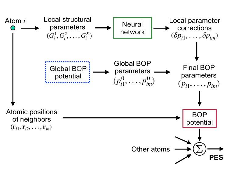
Figure 2: Flowchart of the modified PINN method. The notations are explained in the text.

The diagram in Fig. 2 explains the flow of information in the method. Note that the role of the atomic coordinates $(\mathbf{r}_{i1},\mathbf{r}_{i2},...,\mathbf{r}_{in})$ of the neighboring atoms is twofold: they are arguments of the BOP potential, and they are also used to compute the local structural parameters which, in turn, predict the local corrections $\delta\mathbf{p}_{i}$ to the global BOP parameters $\mathbf{p}^{0}$ after passing through the NN.

In the proposed scheme, the energy predictions are largely guided by the global BOP potential, whose role is to provide a smooth and physically meaningful extrapolation outside the training domain. The magnitudes of the weights and biases of the NN can be controlled to keep the local corrections $\delta\mathbf{p}_{i}$ as small as possible. This approach is designed to improve the transferability of the PINN potential while keeping a high level of accuracy. Tests also show that the modified scheme improves the stability and the speed of convergence during the NN training.

Although the NN is allowed to have any architecture and size, we find that a simple feedforward network with 2 to 3 hidden layers is sufficient for achieving the desired accuracy of training. The input and output layers contain $K$ (number of descriptors) and 8 (number of BOP parameters) nodes, respectively. The loss function has the form

$$\mathcal{E} = \dfrac{1}{N}\sum_{s}\left(\dfrac{E^{s}-E_{\textrm{DFT}}^{s}}{N_{s}}\right)^{2}+\tau_{1}\dfrac{1}{N_{p}}\left(\sum_{\epsilon\kappa}\left|w_{\epsilon\kappa}\right|^{2}+\sum_{\nu}\left|b_{\nu}\right|^{2}\right)$$ (14)

$$+ \tau_{2}\dfrac{1}{N_{a}m}\sum_{s}\sum_{i_{s}=1}^{N_{s}}\sum_{n=1}^{m}\left|p_{i_{s}n}-\overline{p}_{i_{s}n}\right|^{2}+\tau_{3}\dfrac{1}{N_{a}m}\sum_{s}\sum_{i_{s}=1}^{N_{s}}\sum_{n=1}^{m}\left|p_{i_{s}n}\right|^{2}$$

Here $E^{s}$ is the total energy of supercell $s$ predicted by the potential, $E_{\textrm{DFT}}^{s}$ is the DFT energy of this supercell, $N_{s}$ is the number of atoms in the supercell, $N$ is the total number of supercells in the database, $N_{a}$ is the total number of atoms in all supercells, $w_{\epsilon\kappa}$ and $b_{\nu}$ are the weights and biases of the NN, $N_{p}$ is the total number of NN parameters, and $\tau_{1}$, $\tau_{2}$ and $\tau_{3}$ are adjustable coefficients. The first term in the right-hand side is our definition of the mean-square error of fitting. The remaining terms are added for regularization purposes. The second term ensures that the network parameters remain reasonably small for smooth interpolation. The third term controls variations of the BOP parameters relative to their values $\overline{p}_{i_{s}n}$ averaged over the training database. The last term is optional and was added to prevent the BOP parameters from growing beyond physically reasonable limits.

Because of the complex structure of the PINN potential and the loss function, application of the standard NN training methods such as backpropagation is impractical. Instead, we implement the Davidon-Fletcher-Powell algorithm of unconstrained optimization (NRC2, ) in the high-dimensional space of the NN parameters ($N_{p}\gg 1$). This algorithm requires the knowledge of partial derivatives of $\mathcal{E}$ with respect to the NN parameters, which were derived analytically by multi-step application of the chain rule. The global BOP potential is optimized by the same algorithm. The loss function has many local minima, hence the training has to be repeated multiple times starting from different initial conditions. Due to the large size of the optimization problem, the training process relies on massive parallel computations as will be discussed later.

III Development of the PINN potential for Al

III.1 The potential training and validation

The PINN Al potential developed here was trained, validated and tested on the same DFT database as was used in the original version (PINN-1, ). The training and validation database, which we denote $\mathcal{D}$, was composed of DFT energies of 36,490 supercells. These supercells represented seven crystal structures of Al under isotropic and uniaxial tensions and compressions, surfaces with different crystallographic orientations, five symmetrical tilt grain boundaries, unrelaxed intrinsic stacking fault, a vacancy, and several isolated clusters containing from 2 to 79 atoms. Some of the supercells were static (0 K temperature), but most of them were snapshots of DFT MD simulations at different atomic volumes and temperatures. A database $\mathcal{F}\subset\mathcal{D}$ composed of 3,164 supercells (108,052 atoms) randomly selected from $\mathcal{D}$ was created for training purposes. The structures included in the training database $\mathcal{F}$ are described in detail in the Supplementary File accompanying this paper. In addition, 10 more datasets $\mathcal{V}_{i}$, each containing 495 supercells (19,540 atoms), were randomly selected from $\mathcal{D}$ for validation purposes. These validation datasets lay outside the training database ($\mathcal{V}_{i}\subset\mathcal{D}\setminus\mathcal{F}$) and did not intersect with each other ($\mathcal{V}_{i}\cap\mathcal{V}_{j}=\textrm{Ø}$). They were used to control overfitting during the training process. Yet another DFT database $\mathcal{T}$ composed of 26,425 supercells (2,376,388 atoms) was used for testing the potential as will be discussed later. This database was composed of structures different from those in the training and validation database ($\mathcal{T}\cap\mathcal{D}=\textrm{Ø}$). More detailed information about the databases and the DFT calculations can be found in the Supplementary File and in (PINN-1, ).

A number of different descriptors $\mathbf{G}_{i}$, network architectures (including variations in the number of neurons in the hidden layers) and regularization parameters were tested. In each case, the NN weights and biases were initialized by random numbers in the interval [-0.1,0.1]. The optimizer had to be restarted about 10 times with different initial conditions to avoid early trapping in a local minimum. While it was almost always possible to train the model to the same RMSE of about 3 meV per atom, the predicted physical properties varied significantly from one potential to another. Even with all hyper-parameters fixed, the potentials trained to the same RMSE starting from different random sets of weights and biases predicted slightly different sets of physical properties. The final version of the potential selected for this paper was obtained with $\tau_{1}=10^{-4}$, $\tau_{2}=0$, $\tau_{3}=0.02$, $r_{c}=6$ Å, $d=1.5$ Å and $\sigma=1$ Å. The feature vector has the size of $K=40$ corresponding to five Legendre polynomials of orders $l=0,1,2,4$ and 6 with 8 Gaussian positions at $r_{0}=\{2.0,2.5,3.0,3.5,4.0,5.0,6.0,7.0\}$ Å (see Eqs.(10) and (11) for notation). The NN architecture is $40\times 16\times 16\times 8$ with a total of $N_{p}=1064$ fitting parameters. The two hidden layers contain 16 nodes each, and the output layer contains $m=8$ nodes (number of local BOP parameters). The RMSE of training is 2.60 meV per atom. During the training, the RMSE’s of the validation datasets $\mathcal{V}_{i}$ were recorded to make sure that the potential is not subject to overfitting or selection bias. The validation errors continually decreased during the training process, as shown on the convergence plot in the Supplementary File (increase in the validation error would signal overfitting). For the final potential, the RMSE of validation averaged over the 10 validation sets was 3.94 meV per atom.

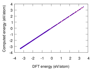
(b)

Figure 3: (a) Energies computed with the PINN potential versus DFT energies for the training database. The straight line represents perfect fit. (b) Error distribution of the PINN potential.

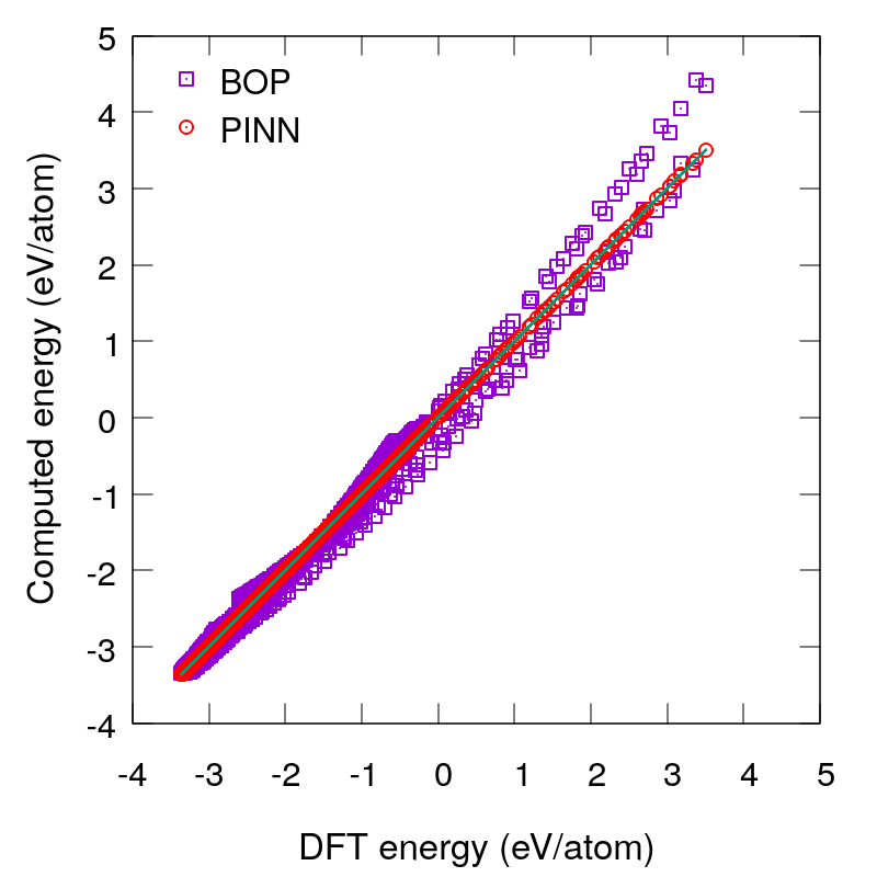
Figure 4: Energies computed with the global BOP potential versus DFT calculations for structures included in the training database. The PINN-DFT plot from Fig. 3 is added for comparison.

Figure 3 shows that the potential predictions are in excellent agreement with the DFT energies uniform across the 7 eV per atom wide energy range. The error distribution is centered at zero (no bias) and has an approximately Gaussian shape. For comparison, Fig. 4 shows the energies predicted by the global BOP potential plotted against the DFT energies. The BOP potential generally follows the DFT trend but is less accurate than the PINN potential and displays significant deviations for some of the high-energy structures. The plot demonstrates the drastic improvement in accuracy achieved by the local adjustments of the BOP parameters implemented in the PINN potential.

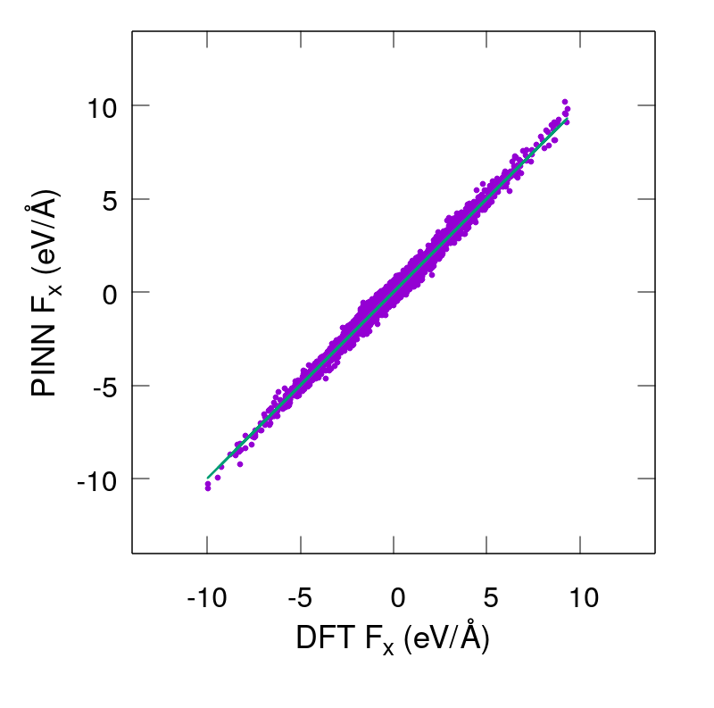
(b)

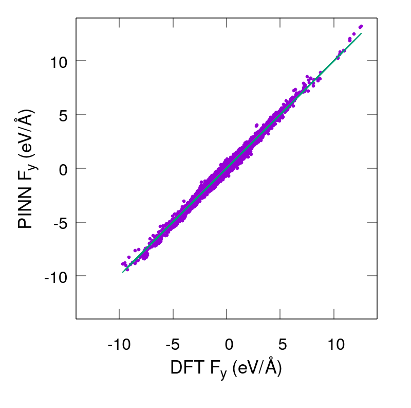
(c)

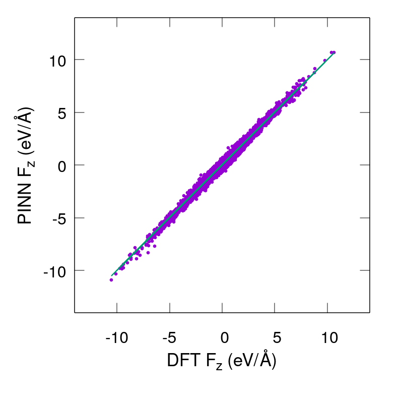
Figure 5: Components of the atomic forces predicted by the PINN potential in comparison with DFT calculations for the training database. The straight lines represent the perfect fit. The RMS deviation is 0.11 eV Å^-1. DFT forces were not used during the potential training and validation.

DFT forces were not used during the training and validation, but they were checked against the potential predictions once the final version was selected. The potential forces display an unbiased scatter relative to the DFT forces with the RMSE of about 0.1 eV Å^-1 (Fig. 5). Forces are sometimes included in the training of ML potentials. This option will be explored with other PINN potentials in the future. In the present case, we chose to examine the forces after the training to demonstrate that the potential was not overfitted (overfitting would manifest itself in a small error in energies and a large error in forces).

III.2 Tests of basic properties

Properties of Al predicted by the PINN potential were computed with the ParaGrandMC (PGMC) code developed at the National Aeronautics and Space Administration (NASA) (ParaGrandMC, ; Purja-Pun:2015aa, ; Yamakov:2015aa, ). The code implements massively parallel MD and MC simulations in a variety of statistical ensembles. It works with several types of interatomic potentials, including the modified PINN potential described in this work. The atomic forces and the stress tensor are computed from analytical expressions. Further details related to this code will be discussed in Section V. The atomic structures appearing in the paper were analyzed and visualized using the Open Visualization Tool (OVITO) visualization tool (Stukowski2010a, ).

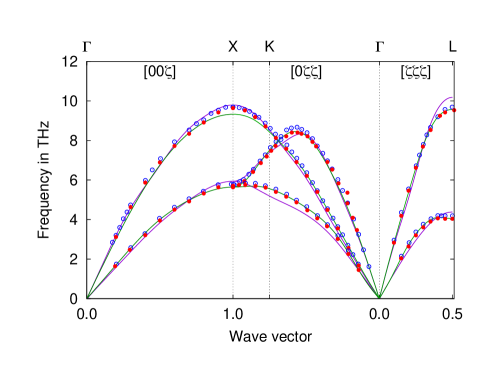
Figure 6: Phonon dispersion curves at 0 K computed with the PINN Al potential (magenta curves) in comparison with DFT calculations (green curves) and experimental data (Stedman:1996aa, ) measured at 80 K (open blue circles) and 300 K (filled red circles).

Table 1 shows that the potential predicts the equilibrium lattice constant $a_{0}$ and the elastic constants $c_{ij}$ of FCC Al in good agreement with DFT values. The potential also demonstrates reasonable agreement with experimental phonon dispersion curves (Fig. 6). The phonon calculationsutilized the phonopy package (phonopy, ) with input from snapshots of a $8\times 8\times 8$ periodic cell generated with the PGMC code. For comparison, the plot also shows the results of DFT calculations performed in this work. We used the Vienna Ab Initio Simulation Package (VASP) (Kresse1996, ; Kresse1999, ) with the Perdew, Burke, and Ernzerhof (PBE) density functional (PerdewCVJPSF92, ; PerdewBE96, ). The calculations used the kinetic energy cutoff of 500 eV, 6 irreducible $k$-points, a Methfessel-Paxton smearing of order 1, and the smearing width of 0.2 eV. The phonopy package (phonopy, ) was utilized with input from a $4\times 4\times 4$ conventional supercell containing 256 atoms with the equilibrium lattice constant of 4.04 Å obtained with the PBE functional. Figure 6 shows that the DFT dispersion curves compare well with the PINN calculations.

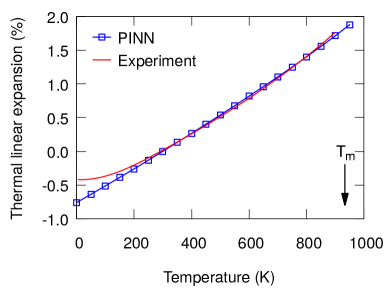
Figure 7: Linear thermal expansion coefficient relative to room temperature predicted by the PINN Al potential in comparison with experiment (the recommended equation approximating the experimental data (Expansion, )). The arrow indicates the experimental melting temperature.

Linear thermal expansion coefficients (relative to 295 K) were computed by MD simulations on a periodic cubic block containing 10,976 atoms. The results compare well with experimental data between 295 K and the melting point (Fig. 7). Deviations at low temperatures are due to quantum effects that cannot be captured by a classical potential.

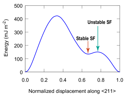
Figure 8: Cross-section of the gamma-surface of Al on the (111) plane computed with the PINN potential. The half-crystal above the (111) plane was incrementally displaced in the [211] direction and the energy was minimized with respect to [111] atomic displacements after each increment. The excess energy is plotted against the displacement normalized by the period of energy in the [211] direction. The displacements corresponding to the stable and unstable stacking faults are indicated. The respective fault energies $\gamma_{SF}$ and $\gamma_{us}$ are indicated in Table 1.

Lattice defect energies in Al are also predicted accurately (Table 1). The surface energies match the DFT values from the literature. Self-interstitial atoms in Al can be localized in octahedral or tetrahedral sites, or form split dumbbell configurations. The potential correctly predicts that the $\left\langle 100\right\rangle$ dumbbell is the most stable configuration. The vacancy migration energy was computed by the nudged elastic band method (Jonsson98, ; HenkelmanJ00, ) and is well within the bracket of the available DFT values. Given that the potential accurately reproduces the point defect energies, it should be suitable for simulations of diffusion, radiation defects, and similar phenomena mediated by point defect energetics and dynamics. The stable and unstable stacking fault energies are in good agreement with DFT data, which is important for simulations of dislocations and grain boundaries. Fig. 8 shows the relevant section of the gamma-surface on the (111) plane, indicating the stable and unstable stacking fault positions.

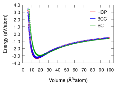
(b)

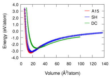
Figure 9: Energy-volume relations for alternate Al structures computed with the PINN potential (lines) in comparison with DFT calculations (points). (a) Hexagonal close-packed (HCP), body-centered cubic (BCC), and simple cubic (SC) structures. (b) A15 (Cr₃Si prototype), simple hexagonal (SH), and diamond cubic (DC) structures.

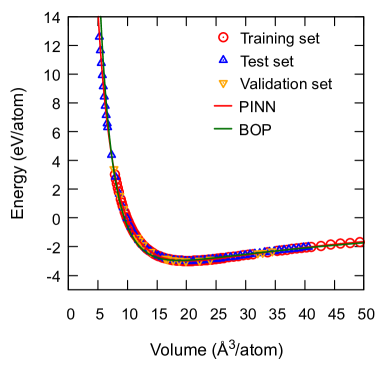
Figure 10: Energy-volume relation for simple cubic Al under strong compression predicted by the PINN and global BOP potentials in comparison with DFT calculations. The triangular symbols represent DFT energies that were not used during the training and validation of the potentials.

Crystal structures other than FCC are also reproduced with high accuracy. In the interval of atomic volumes sampled by the training database, the PINN and DFT energy-volume relations are practically indistinguishable from each other (Fig. 9). Importantly, the agreement continues to be accurate outside the trained volumes. As an example, Fig. 10 examines the energy-volume curves for the simple-cubic structure under strong compression. The PINN potential continues to predict energies that closely match the DFT points that were not included in the training and validation database. This behavior was observed for all crystal structures tested in this work. Note that the global BOP potential also extrapolates well to atomic volumes that were not used during the training and validation. As discussed in Section II, the transferability of the PINN potential owes its origin to the guidance provided by the BOP potential.

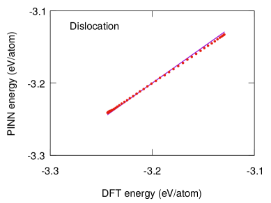
(b)

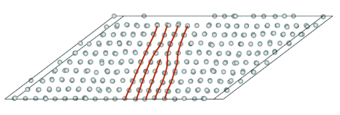
Figure 11: (a) Energy computed with the PINN potential compared with the DFT energy for an edge dislocation in Al at the temperature of 700 K. The straight line represents perfect fit. (b) Supercell containing the edge dislocation viewed along the [211] direction. Selected crystal plans are traced to show the termination of an extra plane.

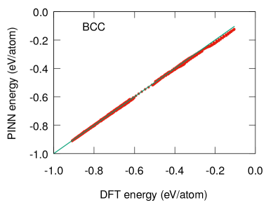
(b)

Figure 12: Energy computed with the PINN potential compared with DFT energy for snapshots of NVT (constant temperature and volume) MD simulations of (a) BCC Al at 1000 K, 2000 K and 4000 K, and (b) HCP Al at 1000 K and 4000 K. The straight line represents perfect fit.

Testing of a potential is an important step that demonstrates its scope of applications. The PINN potential was extensively tested for the ability to reproduce energies of various structures that were not exposed during the training and validation. As mentioned earlier, the testing DFT database $\mathcal{T}$ was in fact larger than the database $\mathcal{F}$$\cup(\cup_{i=1}^{10}\mathcal{V}_{i})$ used for the training and validation. The agreement between the potential predictions and the DFT energies was invariably very good. Examples are shown in Fig. 11 for a dislocation in Al and in Fig. 12 for DFT MD simulations of BCC and HCP structures at three temperatures exceeding the melting point. Due to the small supercell size and the periodic boundary conditions, these crystalline structures were strongly distorted but did not melt even at 4000 K. Note that the training/validation database only included these structures at 0 K. Thus the comparison in Fig. 12 demonstrates the ability of the potential to extrapolate the energy outside the training domain. More tests involving both energies and forces can be found in the Supplementary File.

IV Further tests and applications

IV.1 Calculation of the melting point

In this Section and the subsequent Sections IV.2 and IV.3, the PINN potential will be used to investigate the structure and properties of liquid Al and the solid-liquid coexistence. The motivation for studying systems containing liquid Al in such detail is twofold. Firstly, the knowledge of liquid properties is important for the modeling of technological processes such as alloy casting and additive manufacturing. Secondly, this offers us an opportunity to assess the transferability of the potential to unknown atomic environments. Indeed, the bulk liquid phase was not represented during the training and validation. Almost all structures used during the training and validation were atomically ordered. Some structures were perfectly ordered, others were strongly distorted, but they still maintained a significant degree of long-range order. The only exceptions were the 5 Å (42 atoms) and 6.5 Å (79 atoms) isolated clusters at 1200 K and the Wulff-shape (79 atoms) isolated cluster at 2000 K. These clusters had fully disordered, liquid-like structures. In addition, a trimer put on the (111) surface at 2000 K caused disordering of the surface layer in a 103-atom supercell. However, these disordered structures constituted a small fraction of the database.

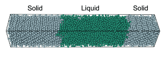
(b)

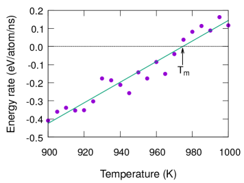
Figure 13: (a) Simulation block containing the solid and liquid phases used for computing the melting temperature. (b) The rate of energy change as a function of temperature in MD simulations of the solid-liquid system. The line is a linear fit to the data. The melting point is the temperature at which the energy rate is zero.

The melting temperature $T_{m}$ predicted by the potential was computed by the interface velocity method described in detail elsewhere (Morris94, ; Morris02, ; Pun09b, ; Purja-Pun:2015aa, ; Howells:2018aa, ). The simulation block had the dimensions of 29 Å$\times$30 Å$\times$185 Å and contained 9,000 atoms, which were partitioned between the solid and liquid phases separated by a (111) interface normal to the long direction. NPT MD simulations (constant temperature and zero pressure) were executed at a series of temperatures near the expected melting point. During the simulations, the solid phase was either melting or crystallizing, depending on whether the chosen temperature happened to be above or below $T_{m}$. Accordingly, the system energy was either increasing with time or decreasing. The rate of the energy change could be converted to the solid-liquid interface velocity to find the temperature at which the velocity vanished. Instead, it was sufficient to monitor the energy rate itself and identify the melting point with the temperature at which this rate was zero. In Fig. 13, the energy rate is plotted against temperature for several simulation runs. Interpolation using a linear regression gives $T_{m}=(975\pm 3)$ K (the uncertainty indicates one standard deviation). We consider the agreement with the experimental melting point of Al (933 K (Kittel, )) encouraging given that it was achieved without any direct fit.

IV.2 Interface tensions

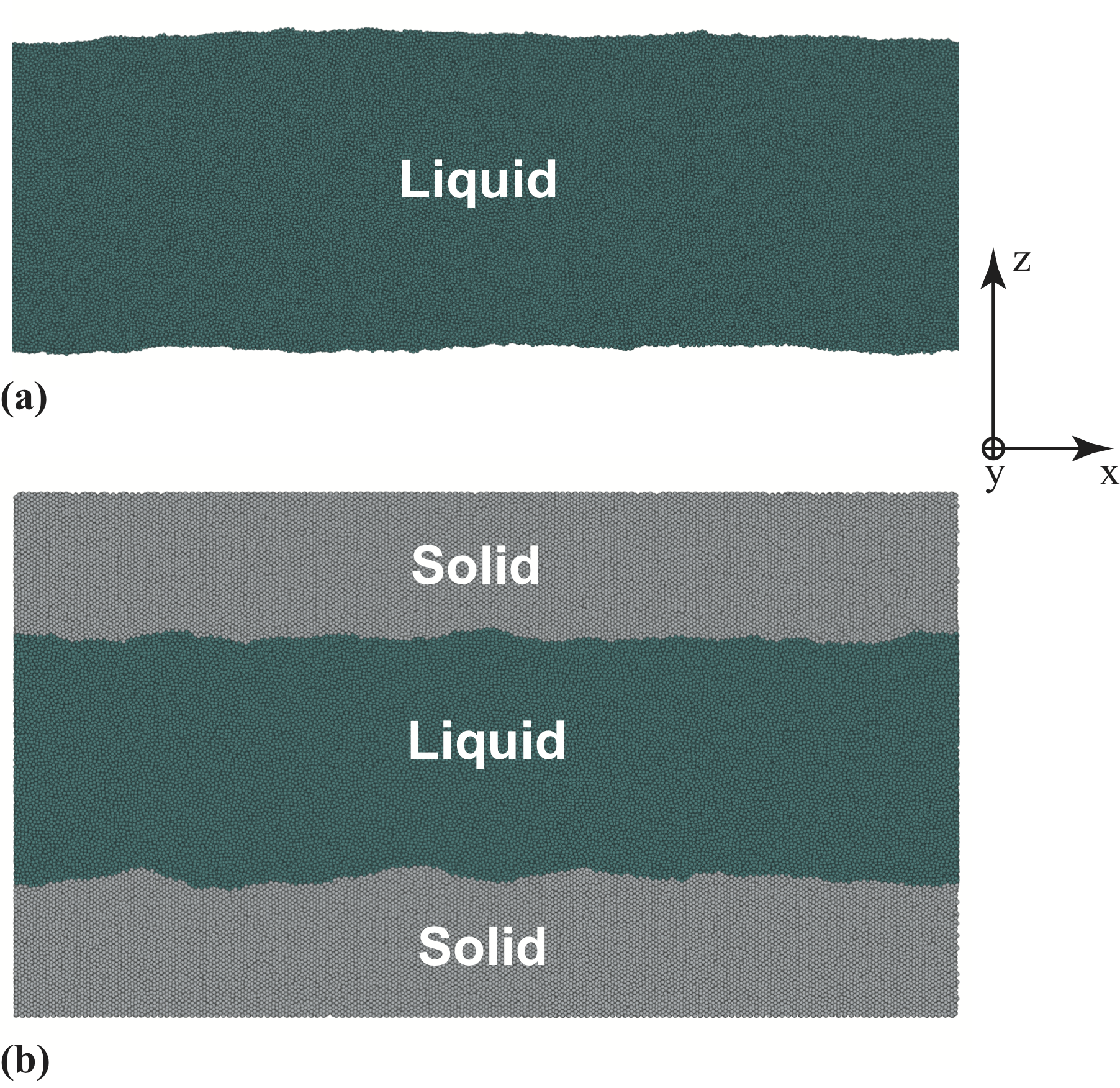
Figure 14: Simulation blocks used for computing the interface tensions in Al. (a) Liquid film with open surfaces. Periodic boundary conditions are applied in the $x$ and $y$ directions. (b) Solid-liquid coexistence system. The crystallographic directions $\langle 100\rangle$ and $\langle 110\rangle$ in the solid phase are parallel to the $x$ and $y$ axes, respectively. Periodic boundary conditions are applied in all three directions. The images are visualized using the potential energies of atoms.

The liquid and solid-liquid interface tensions in Al were computed by the capillary fluctuation method (Hoyt01, ; Morris02a, ; Rozas2011, ; Karma-2012a, ; Mishin2014, ; Asadi2015, ). In this method, the interface is aligned normal to the $z$-direction and has a ribbon-like shape with the $y$-dimension $w$ much smaller than the $x$-dimension $l$. Periodic boundary conditions are imposed in the $(x,y)$ plane. An example is shown in Fig. 14a for liquid surfaces of a free-standing film with $l=622$ Å and $w=29$ Å.

Capillary fluctuations manifest themselves in stochastic variations of the interface shape $z(x)$, which can be quantified by the function $h(x)=z(x)-\overline{z}$, where $\overline{z}$ is the average interface position. Fourier transformation of $h(x)$ gives the power spectrum $|A(k)|^{2}$ of the capillary waves, $A(k)$ being the Fourier amplitude and $k$ the wave number. The canonical expectation value $\left\langle|A(k)|^{2}\right\rangle$ is obtained by averaging the power spectrum over multiple snapshots and the two interfaces present in the system. By fitting $\left\langle|A(k)|^{2}\right\rangle$ with the function (Hoyt01, ; Morris02a, ; Rozas2011, ; Karma-2012a, ; Mishin2014, ; Asadi2015, )

$$\langle|A(k)|^{2}\rangle=\dfrac{k_{B}\,T}{lw\,(\gamma+\gamma^{\prime\prime})\,k^{2}},$$ (15)

the interface stiffness $(\gamma+\gamma^{\prime\prime})$ can be extracted. Here $\gamma$ is the interface tension, $\gamma^{\prime\prime}$ is the second derivative of $\gamma$ with respect to the inclination angle, and $k_{B}$ is Boltzmann’s constant. In practice, $(\gamma+\gamma^{\prime\prime})$ is obtained from the slope of the plot $\left\langle|A(k)|^{2}\right\rangle^{-1}$ versus $k^{2}$ in the long-wave (small $k$) limit.

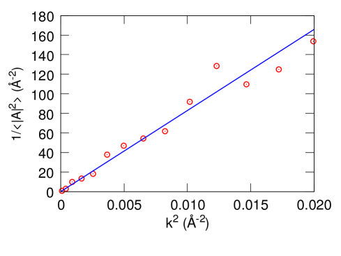
(b)

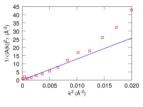
Figure 15: Inverse power of capillary waves versus the wave number squared for (a) liquid Al surface and (b) Al solid-liquid interface computed with the PINN potential. The lines represent linear fits in the long-wave limit.

For computing the liquid surface tension, the simulation block (Fig. 14a) was equilibrated at the melting temperature (975 K) followed by a 0.57 ns long NVE MD production run (constant volume and energy). Snapshots containing the atomic coordinates were saved every 10 ps. At the post-processing stage, each snapshot was divided into 200 thin bins normal to the $x$ axis. The upper and lower interface positions were found by averaging 10 largest (respectively, 10 smallest) $z$-coordinates of atoms in the bin. Because the interfaces are not atomically sharp, the averaging is more appropriate than simply taking the largest and smallest coordinates. The power spectrum of the capillary waves was obtained by a discrete Fourier transformation of the interface locations in the bins. For a liquid surface $\gamma^{\prime\prime}=0$. Linear fit to the $\left\langle|A(k)|^{2}\right\rangle^{-1}$ versus $k^{2}$ plot in the $k\rightarrow 0$ limit (Fig. 15a) gives the surface tension of $\gamma=0.610$ J m^-2.

To verify this result, another, independent method was applied. Namely, the thin film in Fig. 14a is subject to the Laplace pressure $p=2\gamma/d$, where $d=196$ Å is the film width in the $z$-direction. The pressure in the inner region of the film unaffected by the surfaces was computed by averaging over the entire set of snapshots. Knowing the pressure, we obtain $\gamma=pd/2=0.613$ J m^-2 (Table 2). This number is close to the previous result, which lends credence to the capillary wave methodology used in this work. It should be emphasized that the Laplace pressure is mechanical in nature and is caused by the interface stress, whereas the stiffness appearing in the capillary fluctuation method is related to the interface free energy $\gamma$ (which we refer to here as tension). While the interface stress and interface free energy are conceptually different properties, they are numerically equal for a liquid surface. It is this equality that enabled us to compute the same surface tension by the two different methods. This cannot be done for the solid-liquid interface discussed below, for which the interface stress and interface free energy (tension) are generally different (Willard_Gibbs, ; Cahn79a, ; Cammarata1994b, ; Cammarata08, ; Frolov09, ; Frolov2010b, ).

For comparison, the same calculations were performed with one of the widely used EAM Al potentials (Mishin99b, ). The melting temperature predicted by this potential is 1042 K (Ivanov08a, ). A larger simulation block could be afforded thanks to the computational efficiency of the EAM. The $\left\langle|A(k)|^{2}\right\rangle^{-1}$ versus $k^{2}$ plot can be found in the Supplementary File. Although the EAM potential is expected to be less accurate than the PINN potential, the surface tensions obtained are reasonably close to the respective PINN values (Table 2). For completeness, Table 2 also cites experimental data (Poirier:1987aa, ; Egry:2008aa, ). The experimental surface tension tends to be higher than the computed ones. However, comparison with experiment should be taken with caution. Experimental measurements are conducted on much larger droplets, typically several millimeters in radius (Schmitz:2009aa, ; Zhao:2017aa, ; Poirier:1987aa, ; Egry:2008aa, ). The tension is extracted from droplet shape oscillations during electromagnetic levitation. The accuracy of the results is limited by many factors, such as temperature control, surface contamination and evaporation.

Solid-liquid interfaces were created in a simulation block containing both phases in thermodynamic equilibrium with each other at the melting temperature of the respective potential (Fig. 14b). The interfaces were parallel to the (110) plane of the solid phase, with periodic boundary conditions imposed in all three directions. To ensure zero pressure, the lattice constant of the solid phase was adjusted according to the thermal expansion coefficient at the chosen temperature. The system size in the $z$-direction was also adjusted to remove the normal stress. Once thermodynamic equilibrium was reached, a production run was implemented in the NVE MD ensemble for 0.57 ns (PINN) or 10 ns (EAM). To compute the interface shape, the liquid phase in each snapshot was “removed” by discarding all atoms whose energy was greater than -3.142 eV. The surfaces of the remaining solid mimicked the solid-liquid interfaces, which were then binned to determine the $z$-coordinates of the interfaces positions as discussed above. The remaining steps were the same as for the liquid surfaces.

Figure 15b shows the $1/\langle|A(k)|^{2}\rangle$ versus $k^{2}$ plot computed with the PINN potential (see Supplementary File for the plot obtained with the EAM potential). The interface stiffness obtained is 95 mJ m^-2 (Table 3), which is almost an order of magnitude smaller than the liquid surface tension. Since the calculations were performed for a single interface orientation, the interfaces tension $\gamma$ cannot be separated from the torque term $\gamma^{\prime\prime}$. Thus only the stiffness values $(\gamma+\gamma^{\prime\prime})$ are reported. The stiffness predicted by the EAM potential (Mishin99b, ) is slightly higher but close to the PINN result (Table 3). Taken together with the liquid surface results, we observe that the EAM potential (Mishin99b, ) tends to overestimate the interface tensions but otherwise demonstrates reasonable accuracy. Other authors reported even larger stiffness values using different EAM (Morris02a, ) and MEAM (Asadi2015, ) potentials. Comparison with experiment is problematic. The solid-liquid interface stiffness has only been estimated by indirect methods, such as back-calculation from experimentally observed crystal nucleation rates, measurements of dihedral angles (this requires the knowledge of other tensions), or melting point depression (Jiang08, ). The anisotropy of stiffness is not taken into account. Nevertheless, some experimental data is included in Table 3 for completeness.

IV.3 Liquid structure and properties

We next discuss the structure and properties of liquid Al as a single phase. Two structural properties will be examined: the radial distribution function (RDF) and the bond angle distribution.

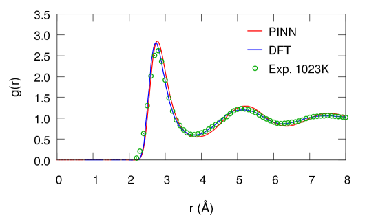
(b)

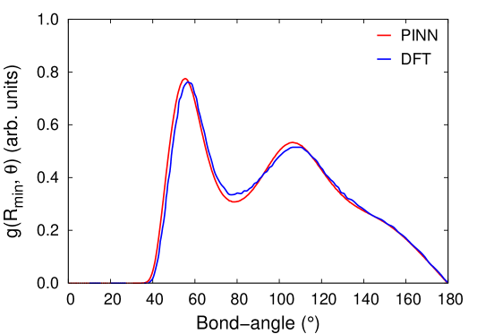
Figure 16: Structure of liquid Al at 1000 K predicted by the PINN potential in comparison with experimental data (Mauro:2011wc, ; Jakse:2013aa, ) and DFT calculations (Alemany:2004, ; Jakse:2013aa, ). (a) Radial distribution function; (b) bond-angle distribution function.

The RDF $g(r)$ was computed by averaging over 250 snapshots saved during a 30 ps NPT MD simulation at several temperatures. The simulation block contained 10,976 atoms with periodic boundaries. Figure 16a shows the RDFs at the temperatures of 1000 K (PINN and DFT) and 1013 K (experiment). Similar plots for the temperatures of 875 K, 1125 K and 1250 K are included in the Supplementary File. In all cases tested, the results predicted by the PINN potential were in very good agreement with both experimental data and DFT calculations (Mauro:2011wc, ; Jakse:2013aa, ).

The same MD snapshots were used to compute the distribution function $g(R_{\textrm{min}},\theta$) of bond angles $\theta$. The bonds were defined as vectors connecting a chosen atom with its neighbors lying within the radius $R_{\textrm{min}}$ of the first minimum of $g(r)$. The function $g(R_{\textrm{min}},\theta$) obtained (Fig. 16b) compares well with the results of DFT MD simulations (Alemany:2004, ).

Calculations of density, viscosity and diffusivity were performed at 10 temperatures ranging from 1050 K to 1500 K at 50 K intervals using a periodic cubic block containing 32,000 atoms. At each temperature, the system was equilibrated by an NPT MD simulation for at least 200 ps to ensure decorrelation from the previous temperature and reach the equilibrium density. The equilibration was followed by 20 to 30 production runs, 100 ps each, implemented in the NPT ensemble for density calculations and NVT ensemble for computing the viscosity and diffusivity. The MD integration step was 1 fs. The atomic stress, atomic positions, velocities, energies, and other relevant parameters were measured at every MD step. The viscosity and diffusion coefficients were computed by the Green-Kubo method following the methodology described in Ref. (Mondello:1997aa, ). As a cross-check, the diffusion coefficients were also computed from mean-squared atomic displacements using the Einstein equation.

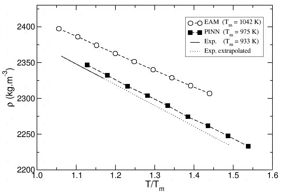
Figure 17: Density of liquid Al as a function of homologous temperature $T/T_{m}$ computed with the PINN and EAM (Mishin99b, ) potentials in comparison with experimental data (Assael:2006aa, ).

Figure 17 shows the temperature dependence of the liquid density computed with the PINN and EAM (Mishin99b, ) potentials and measured experimentally (Assael:2006aa, ). To facilitate comparison, the homologous temperature ($T/T_{m}$) is used as the melting points predicted by the potentials are shifted relative to the experiment. The PINN potential is clearly in better agreement with experiment than EAM.

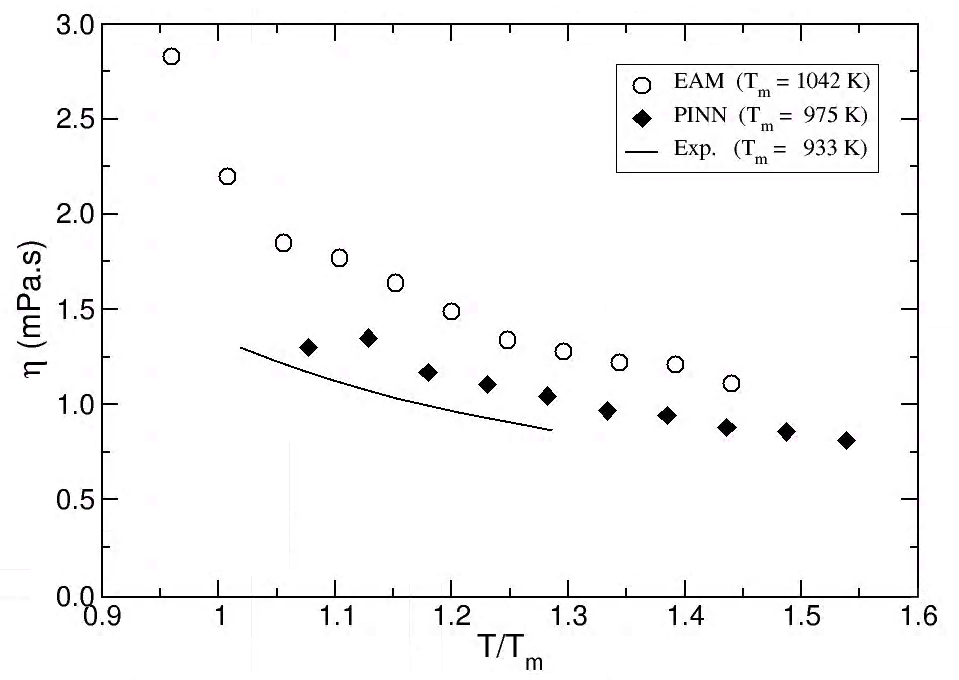
(b)

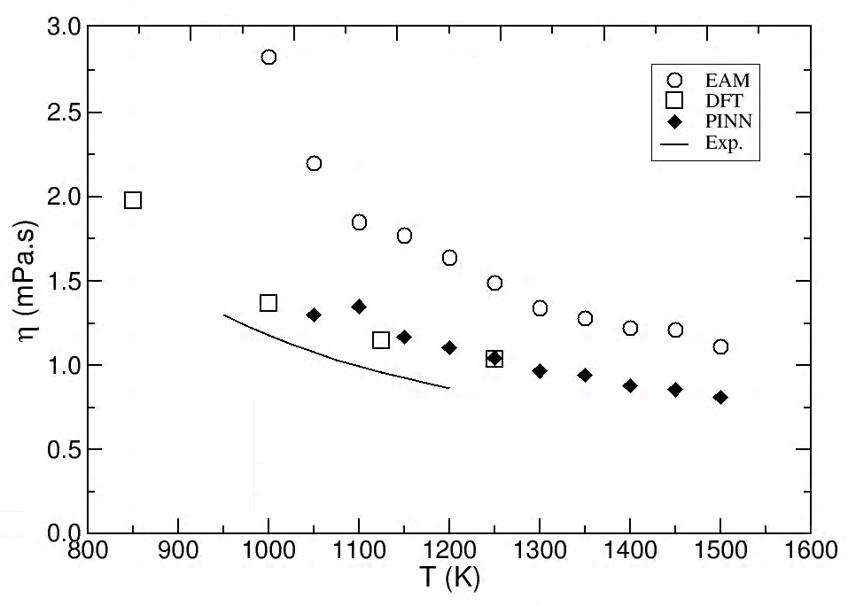
Figure 18: Viscosity of liquid Al as a function of temperature computed with the PINN and EAM (Mishin99b, ) potentials in comparison with (a) experimental data (Assael:2006aa, ) using the homologous temperature $T/T_{m}$, and (b) DFT calculations (Jakse:2013aa, ) using the actual temperature.

For viscosity, the agreement with experiment (Assael:2006aa, ) is similarly good as illustrated in Fig. 18a. Furthermore, our results can be compared with DFT data reported by Jakse et al. (Jakse:2013aa, ). Their calculations were performed in both the local density approximation (LDA) and the generalized gradient approximation (GGA). We choose the GGA data for comparison because the DFT database (Botu:2015aa, ; Botu:2015bb, ; PINN-1, ) utilized for training and validation of the PINN potential was generated in the GGA. We use the actual (not homologous) temperature because the DFT melting temperature is unknown. Figure 18b demonstrates that the PINN calculations are in excellent agreement with the DFT data.

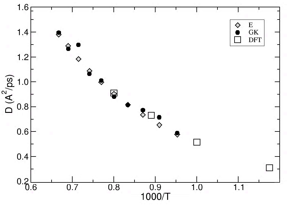
Figure 19: Arrhenius diagram of self-diffusion coefficients in liquid Al computed with the PINN potential using the Green-Kubo (GK) and Einstein (E) methods in comparison with DFT calculations (Jakse:2013aa, ).

Finally, the Arrhenius diagram of diffusion coefficients in liquid Al is shown in Fig. 19. Excellent agreement is observed between the diffusivities obtained by the Green-Kubo and Einstein methods. Equally good is the agreement between the PINN and DFT calculations (again, using the GGA data) across the temperatures covered by the simulations. Comparison with experiment has not been attempted because the existing experimental data is not reliable enough for a meaningful comparison. Accurate self-diffusion measurements are made with stable or radioactive isotopes. Aluminum does not have a suitable isotope for diffusion measurements. Hence the diffusivities reported in the literature were obtained by indirect methods that are less reliable.

IV.4 Grain boundary crack growth

To further demonstrate the possibility of conducting large-scale simulations with PINN potentials, we performed simulations of a bicrystal containing a crack growing on a grain boundary (GB) subject to an applied stress. The system setup closely follows the one reported in a previous paper (Yamakov06, ), where an EAM Al potential was used. Relying on an already studied system helped us in establishing the correct loading conditions ensuring a continuous crack growth after nucleation.

Crystallographic orientations of the two grains are $x:[\overline{7}\thinspace 7\thinspace 10]$, $y:[5\thinspace\overline{5}\thinspace 7]$, $z:[1\thinspace 1\thinspace 0]$ in the upper grain and $x:[\overline{7}\thinspace 7\thinspace 10]$, $y:[\overline{5}\thinspace 5\thinspace\overline{7}]$, $z:[1\thinspace 1\thinspace 0]$ in the lower grain. Thus, the two lattices are mirror images of each other with respect to the GB plane $\left\{5\thinspace 5\thinspace 7\right\}$. This GB is classified as $\Sigma 99$ $[1\thinspace 1\thinspace 0]$ symmetrical tilt boundary with the misorientation angle of $89.42^{\circ}$ ($\Sigma$ is the reciprocal density of coincident sites and $[1\thinspace 1\thinspace 0]$ is the tilt axis). The atomic structure of this boundary is known from previous simulations and observations by atomic-resolution electron microscopy (Dahmen:1990aa, ). The system thickness in the $z$-direction is 10 $\left\{2\thinspace 2\thinspace 0\right\}$ crystallographic planes ($\sim 29$ Å). This thickness is more than a factor of 4 larger than the cutoff radii of the PINN and EAM potentials tested here, preventing interactions of atoms with their periodic images and preserving the local three-dimensional physics. The system dimensions in the $x$ and $y$ directions are 530 Å and 497 Å, respectively, and the total number of atoms is 427,333.

Following thermal equilibration at the temperature of 100 K and zero pressure, the system was loaded hydrostatically in tension to 4 GPa and re-equilibrated at this stress. Once equilibrium was established between the strain in the system and the applied external stress, the system size in all three dimensions was fixed, creating a constant strain condition. To save computer time, the equilibration steps were first implemented with the EAM potential (Mishin99b, ). Transition to the PINN potential was accomplished by an additional simulation at constant temperature and strain for about 20 ps. After reaching equilibrium with the PINN potential, a crack was nucleated by cutting atomic interactions between atoms across the GB plane in 100 Å long region. This length is larger than the Griffith length, $L_{G}\approx 53$ Å, estimated for these loading conditions (Yamakov06, ). This condition ensures that the crack will nucleate and grow, rather than shrink and disappear.

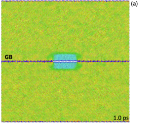
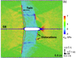
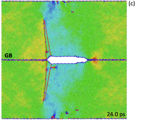
Figure 20: MD simulation of crack nucleation and growth on a $\Sigma 99$ $[1\thinspace 1\thinspace 0]$ symmetrical tilt boundary in Al performed with the PINN Al potential. (a) Early stage after crack nucleation; (b) Crack shape after 6.6 ps of growth; (c) End of the crack growth at 24 ps after nucleation. Visualization of dislocations and twins is based on common neighbor analysis superimposed on a tensile stress map using the opens source code OVITO (Stukowski2010a, ).

The snapshots in Figure 20 represent the crack configurations from the early stages of the simulation and during the growth for 24 ps of NVT MD time. The snapshots combine structural common neighbor analysis (CNA) to identify the dislocations and twins, with the tensile stress field given as a background. The simulation took approximately 14 h of CPU time on a CPU-GPU system described in the next Section. The crack growth follows different mechanisms of propagation at the two crack tips, depending on the inclination of (111) slip planes with respect to the crack growth direction, such as the deformation twinning on the left and dislocation emission on the right. The results are fully consistent with the theoretical analysis (Yamakov06, ) predicting the different crack propagation mechanisms (dislocation emission versus cleavage) based on the Rice criterion (Rice1992, ). While the present simulations did not show notable differences from the results in Ref. (Yamakov06, ), they illustrate the capability of the PINN potential to be used in simulations of the same scale as with the traditional potentials such as EAM.

V Computational efficiency

The greatest advantage of ML potentials is their ability to accelerate and upscale atomistic simulations relative to straight DFT calculations while keeping a near-DFT level of accuracy in predicting the energy and forces. A detailed comparison of computational performance of ML potentials has recently been published (Zuo:2020aa, ). Like other ML potentials, the PINN potentials scale linearly with the number of atoms and are much faster than DFT calculations, but of course slower than traditional potentials. Specific numbers depend not only on the particular potential but also on the simulation software and computer hardware. A few examples discussed below are only intended to give a general idea about the computational efficiency of PINN. These numbers may vary if a different simulation package and/or a different computer architecture are used.

The training of the PINN Al potential reported here was performed using an in-house code written in the C/C++ programming language and parallelized with the Message Passing Interface (MPI). A typical training run engaged 400 Central Processing Units (CPU) ((20 nodes)$\times$(20 cores each)) and took about an hour to complete 200 optimization iterations. A complete optimization down to (2 to 3) meV per atom typically required more than 4,000 iterations. As mentioned above, the optimization had to be repeated multiple times to find an optimal combination of physical properties and perform cross-validation.

The MD simulations were performed with a version of the PGMC code (ParaGrandMC, ; Purja-Pun:2015aa, ; Yamakov:2015aa, ). The code is parallelized by implementing a spatial decomposition that distributes the system over a number of compute nodes connected through MPI. On each node, an Open Multi-Processing (OpenMP) programming interface was used to distribute the calculations over the available CPU cores. When a Graphic Processing Unit (GPU) was available, the Open Accelerators (OpenACC) programming interface was used to upload part of the calculations on the GPU. In this case, the search for neighbors within the cutoff range was performed with OpenMP taking advantage of all CPU cores, while the energy and force calculations were uploaded to the GPU using OpenACC. Accordingly, two computing configurations were used with a similar performance: A CPU-only configuration, and a CPU-GPU configuration. The latter consisted of a single node equipped with two dual socket 20 core Intel Gold 6148 Skylake CPU cores running at 2.40 GHz with 4 Nvidia V100 GPU cards (total: CPUs = 40, GPUs = 4). To utilize the node architecture efficiently, MPI was used to spatially decompose the system into 4 subdomains and represent the compute node as 4 MPI nodes with 10 CPU cores and one GPU card each.

MD calculations of the melting point, interface tensions and the liquid structure were conducted in the CPU-only mode using a single node composed of 28 cores (1 MPI process with a total of 56 threads). A typical MD simulation of 10,976 atoms took about 24 hrs to complete 40,000 MD steps (40 ps). In the liquid density, viscosity and diffusion calculations, a 120 ps MD simulation took 47 to 72 CPU hrs (depending on the machine load) using either the CPU-only configuration (8 MPI nodes of 16 cores each) or the CPU-GPU configuration as already described. Both configurations showed a similar computational performance. In the GB crack simulation (427,333 atoms), the 24 ps MD simulation (12,000 MD steps) took about 14 hrs on the CPU-GPU system.

To evaluate the PINN efficiency relative to traditional potentials, the EAM Al potential (Mishin99b, ) was used as an example. With the same PGMC code and the same computer hardware, the EAM potential was found to be about a factor of 170 faster. Most of the overhead time of PINN (about 65 %) is spent on computing the local structural descriptors. This step is common to all ML potentials, including the purely mathematical NN potentials mentioned in Section I. The additional overhead due to the incorporation of the BOP potential in PINN constitutes about 25 % of the total time. The NN calculations are the fastest taking less than 10 % of the compute time. For comparison, the integration of the equations of motion using the velocity Verlet integrator take less than 0.1 % of the compute time. Given the benefits of the PINN approach discussed in the paper, we believe that this modest overhead (about 25 %) is worth its value.

VI Conclusions

The PINN model (PINN-1, ) has been modified to accelerate the potential training process and improve the transferability. Instead of predicting the BOP parameters directly, the NN now predicts local corrections to fixed parameters of a global BOP potential pre-trained on the same DFT database. Such corrections (perturbations) play a supporting role, whereas the physics-based global BOP potential takes the lead in guiding the energy and forces. The on-the-fly adaptivity through local corrections drastically improves the accuracy of the potential, as illustrated by the BOP-PINN comparison in Fig. 4. As long as the corrections remain relatively small, transferability to unknown atomic environments must be robust. Of course, as with any model, the PINN model eventually fails when the atomic configurations arising during the simulations drift too far away from the training domain and the predicted BOP parameters become unphysical. However, the incorporation of physics through the BOP potential significantly expands the range of validity of the potential in comparison with purely mathematical ML potentials.

As an application, a general-purpose Al potential has been constructed following the modified PINN formalism. The potential accurately reproduces the training DFT database (RMSE < 3 meV per atom) over a 7 eV per atom wide energy range as shown in Fig. 3. By contrast to most of the existing ML potentials, the PINN potential has been tested for a wide spectrum of physical properties. In fact, it has been tested at least as thoroughly as traditional potentials are normally tested prior to release to users. However, by contrast to traditional potentials, the PINN Al potential demonstrates much higher accuracy comparable to that of DFT calculations. The tests have shown that the potential faithfully reproduces many properties of Al obtained by DFT calculations (mostly collected from the literature). When appropriate, comparison with experiment has been made and the agreement was found to be reasonable. It should be noted that deviations from experiment are partially accounted for by the fact that the potential was trained on DFT data without any experimental input. DFT calculations would not necessarily reproduce the experiment accurately either. We include the comparison with experiment primarily to inform those users who will be mainly interested in the ability of the potential to reproduce or predict experimental data. This is often the case in simulations geared towards practical applications.

The capability of the potential to perform large-scale simulations has been demonstrated by computing the melting temperature of Al, the structure and dynamic properties of liquid Al, the interface tensions by the capillary fluctuation method, and the nucleation and growth of a grain boundary crack. Some of these simulations involved tens or hundreds of thousands of atoms and/or required MD runs for hundreds of picoseconds. It should also be emphasized that these simulations explored atomic environments that were significantly different from those represented in the training database. As such, they mainly occurred in the extrapolation regime.

Computational efficiency of ML potentials is an important factor that drives their development and applications. ML potentials are orders of magnitude faster than straight DFT calculations, but of course slower than traditional potentials. Specifically, the PINN Al potential developed here is estimated to be two order of magnitude slower than a typical EAM potential. To maintain access to the same size of simulations, more powerful computational resources and more efficient training and simulation codes must be developed. Using the PGMC simulation code as an example, it has been demonstrated that this goal can be achieved by a proper combination of parallel programming interfaces highly optimized for the available computer architectures.

The current work includes the incorporation of PINN potentials into other large-scale simulation packages, such as the Large-scale Atomic/Molecular Massively Parallel Simulator (LAMMPS) (Plimpton95, ), construction of PINN potentials for other metallic and nonmetallic materials, and the development of a multi-component version of PINN. In the latter case, the size $K$ of the feature vector $(G_{i}^{1},G_{i}^{2},...,G_{i}^{K})$ grows as the number of chemical components squared, which is a common property of all ML potentials. The number of BOP parameters also scales up in the same proportion, resulting in a drastic increase in the number of weights and biases in the network. The size of the training database must also be much larger to properly represent different chemical compositions of the system. Even the development of a binary PINN potential is a demanding task, but can still be accomplished given sufficient computational resources. Several ML potentials for binary and ternary systems have already been been reported in the literature (Artrith:2011ab, ; Artrith:2011aa, ; Sosso2012, ; Artrith:2016aa, ; Artrith:2017aa, ; Hajinazar:2017aa, ; Kobayashi:2017aa, ; Artrith:2018aa, ; Li:2018aa, ; Hajinazar:2019aa, ; Gubaev:2019aa, ; Zhang:2019ab, ).

Table 1: Aluminum properties predicted by the PINN potential in comparison with experimental data and DFT calculations. $E_{0}$ - equilibrium cohesive energy, $a_{0}$ - equilibrium lattice parameter, $B$ - bulk modulus, $c_{ij}$ - elastic constants, $\gamma_{s}$ - surface energy, $E_{v}^{f}$ - vacancy formation energy, $E_{v}^{m}$ - vacancy migration barrier, $E_{I}^{f}$ - interstitial formation energy for the tetrahedral ($T_{d}$) and octahedral ($O_{h}$) positions and split dumbbell configurations with different orientations, $\gamma_{\textrm{SF}}$ - intrinsic stacking fault energy, $\gamma_{\textrm{us}}$ - unstable stacking fault energy. All defect energies are statically relaxed unless otherwise indicated.

Property		DFT		PINN
$E_{0}$ (eV per atom)		3.7480a		3.3604
$a_{0}$ (Å)		4.039a,d; 3.9725–4.0676c		4.0399
$B$ (GPa)		83a; 81f		81
$c_{11}$ (GPa)		104a; 103–106d		112
$c_{12}$ (GPa)		73a; 57–66d		65
$c_{44}$ (GPa)		32a; 28–33d		28
$\gamma_{s}$(100) (J m-2)		0.92b		0.904
$\gamma_{s}$(110) (J m-2)		0.98b		0.954
$\gamma_{s}$(111) (J m-2)		0.80b		0.804
$E_{v}^{f}$ (eV)		0.6646–1.3458c; 0.7e		0.703
$E_{v}^{f}$ (eV) unrelaxed		0.78e		0.76
$E_{v}^{m}$ (eV)		0.3041–0.6251c;		0.628
$E_{I}^{f}$ ($T_{d}$) (eV)		2.2001–3.2941c		2.760
$E_{I}^{f}$ ($O_{h}$) (eV)		2.5313–2.9485c		2.739
$E_{I}^{f}$ $\langle$100$\rangle$ (eV)		2.2953–2.6073c		2.517
$E_{I}^{f}$ $\langle$110$\rangle$ (eV)		2.5432–2.9809c		2.843
$E_{I}^{f}$ $\langle$111$\rangle$ (eV)		2.6793–3.1821c		2.775
$\gamma_{\textrm{SF}}$ (mJ m-2)		134i; 145.67g; 158h		134
$\gamma_{\textrm{us}}$ (mJ m-2)		162j; 175h		150
a Ref. (Jong:2015fk, ); b Ref. (Tran:2016qq, ); c Ref. (Qiu:2017ve, ); d Ref. (Zhuang:2016, ) e Ref. (Iyer:2014, );
f Ref. (Sjostrom:2016, ); g Ref. (Devlin:1974qp, );h Ref. (OgataLY02, ); i Ref. (Jahnatek:2009aa, ); j Ref. (Kibey:2007aa, )

Table 2: Surface tension of liquid Al predicted by the PINN and EAM (Mishin99b, ) potentials at the respective melting temperatures. Experimental results measured on microscopic droplets are included for comparison.

Method	System size	Number of atoms	$\gamma$ (J m-2)
			Capillary waves	Laplace pressure
PINN	622 Å$\times$29 Å$\times$196 Å	186,000	0.610	0.613
EAM	619 Å$\times$29 Å$\times$359 Å	360,000	0.717	0.738
Experiment	$\approx$mm		0.828a; 0.87b
a Ref. (Poirier:1987aa, )
b Ref. (Egry:2008aa, )

Table 3: The stiffness $(\gamma+\gamma^{\prime\prime})$ of the solid-liquid interface in Al computed with the PINN and EAM potentials at the respective melting temperatures. Experimental data is included for comparison.

Method	System size	Number of atoms	$(\gamma+\gamma^{\prime\prime})$ (mJ m-2)
PINN	622 Å$\times$29 Å$\times$364 Å	360,000	95
EAM (Mishin99b, )	619 Å$\times$29 Å$\times$359 Å	360,000	99
Other calculations			110a; 135.2b
Experiment			$158\pm 30$c; 131-153d
a Ref. (Morris02a, ) (EAM)
b Ref. (Asadi2015, ) (MEAM)
c Ref. (Jiang08, ) (Dihedral angle)
d Ref. (Jiang08, ) (Melting point depression)

(a)

(a)

(a)

(a)

(a)

(a)

(a)

(a)

(a)

(a)