Causal cosmology with braneworld gravity including Gauss Bonnet coupling

Abstract

Causal cosmological evolutions in Randall Sundrum type II (RS) braneworld gravity with Gauss Bonnet coupling and dissipative effects are discussed here. Causal theory of dissipative effects are illustrated by Full Israel Stewart theory are implemented. We consider the numerical solutions of evolutions and analytic solutions as a special case for extremely non-linear field equation in Randall Sundrum type II braneworld gravity with Gauss Bonnet coupling. Cosmological models admitting Power law expansion, Exponential expansion and evolution in the vicinity of the stationary solution of the universe are investigated for Full Israel Stewart theory. Stability of equilibrium or fixed points related to the dynamics of evolution in Full Israel Stewart theory in Randall Sundrum type II braneworld gravity together with Gauss Bonnet coupling are disclosed here.

Received (Day Month Year)Revised (Day Month Year)

PACS Nos.: 98.80.Jk;98.80.Es.

1 Introduction

Recent observational data suggest an accelerated expanding universe at the present epoch [1, 2]. These cosmological observations also recommend a specially flat universe with high accuracy. To cosmologist, it is a challenging theoretical problem to recognize the precise motivation for the present accelerated expansion. It is proposed that in the early universe there might be a phase of inflationary evolution. Theoretically inflation is understood considering scalar field of standard model. Inflaton are addressed by Starobinsky [3, 4] long ahead of beginning of inflation [5] is recognized. However, in standard model the essential fields for present acceleration are inaccessible. To address the present epoch the motivation of dark energy including dark matter is established. According to PLANCK Collaboration[6] the contribution of dark energy is $\sim$ 69.4$\%$ and that of matter parts (mainly dark matter) are $\sim$ 30.6 $\%$ of total energy. At present, it is one of the most challenging problem to address the dark universe in which dominating parts are dark matter and dark enrgry. The appraisal of extensions of general theory of relativity (GTR) are considered to tackle the challenging issues of the dark universe. Some proposals[7, 8] are introduced by literature to realize the accurate basics of the dark universe. Modified gravity such as Gauss Bonnet [9, 10] gravity, $f(T)$[11, 12] gravity , $f(R)$ [13, 14] gravity, $f(R,T)$ [15, 16, 17] gravity and Horava-Lifshitz [18, 19] gravity are considered to realize the problem. Literature [20] also consider another interesting and important modified theory of gravity known as braneworld gravity.

In braneworld scenario [21, 22], particles of standard model are restricted on brane surrounded by extra dimension bulk. In bulk matter and gravity can only transmit. Randall Sundrum type II braneworld [23, 24] gravity of five dimension can simply illustrate such circumstances. The Superstring/ M-theory motivated such Randall Sundrum model of braneworld gravity. The early stage of universe described by Randall Sundrum typre II braneworld gravity can afford innovative type of evolution. In the brane theory, the five dimensional anti de Sitter space known as bulk surrounded practical universe is considered as four dimensional brane. In a Randall-Sundrum type II scenario (RS II), spatially homogeneous and isotropic brane can be present in the extra dimensional anti de Sitter (AdS₅) bulk spacetime [25]. At low energy the extra dimension support to detain graviton close to brane, so the general theory of relativity are recovered. However, at high energy extra dimension dominate as a result the graviton localization falls short that support a modification of Friedmann equations. The conformal field [26, 27] theory also support this characteristics. A conformal field theory [28, 29] coupled with normal gravity is counterpart of the Randall-Sundrum braneworld theory.

Einstein Hilbert (EH) action of five dimension support the Randall Sundrum braneworld gravity. The EH action can attain quantum improvement at high energies. To extend the braneworld theory further in string theoretical background, it is essential to take account of curvature invariant term ($R,\;R_{ab}R^{ab},R_{abcd}R^{abcd},..$) in the bulk action [30, 31]. Within these modifications, the so called Gauss-Bonnet term can be included. The Gauss-Bonnet (GB $=R_{abcd}R^{abcd}-4R_{ab}R^{ab}+R^{2}$, symbols usual significance) term has merely second derivatives of the metric of equation of motion which is ghosts [32, 33] free and therefore important [34, 35] to consider. The most important quantum improvement in the heterotic string efficient action [36, 37] shows Gauss Bonnet term. In EH bulk action [38, 39] with the presence of Gauss Bonnet term zero mode of gravitation localization on the brane is permitted. It is also found that the Gauss-Bonnet term have a tendency to reduce the limitation of Randall Sundrum braneworld theory. Extensive studies of the Gauss-Bonnet brane world scenario [40, 41] are considered to explain both the early inflation and the late acceleration [42].

Cosmological models with perfect fluid as a source of matters are considered in modified gravity theories. Modified theories of gravity without de Sitter solution or matter admitting inflation is unstable. Although perfect fluid satisfactorily describe matter sharing of the observed universe, however, the evolution of the universe in many phases guide to viscosity [43]. Viscosity may arises in different phases of evolution namely, radiation epoch, recombination epoch, superstrings in quantum epoch, graviton involved collision epoch, galaxies formation epoch [44, 45, 46, 47]. Therefore, it is necessary to incorporate viscosity in the evolution of the universe. Eckart [48] theory is the first theory of viscosity, where concept of non equilibrium thermodynamics is used in relativistic framework. However, Eckart [48] theory suffers from causality and stability conditions. Israel and Stewart [49] extend a fully relativistic foundation of the viscous theory considering second order deviation term to overcome the shortcomings. In Israel and Stewart formalism phantom solution is also investigated in literature [50]. In this paper, we provide an development of the RS brane-world model incorporating viscosity and Gauss Bonnet (GB) term in EH bulk action. The paper is planned as: In section 2, relevant field equations in Randall Sundrum type II (RS) braneworld theory are set up with Gauss Bonnet (GB) term and viscosity. In section 3, we obtain cosmological evolution in RS brane gravity with Gauss Bonnet (GB) term and causal viscous theory. Stability analysis of the causal solution is also considered here. Finally, in sec. 4, we summarize the results.

2 Relevant field equation for braneworld gravity

The 5D Einstein Hilbert (EH) bulk action with GB term and 4D brane yields

$$S=\frac{1}{2k_{5}^{2}}\int d^{5}x\sqrt{-g_{5}}\left[-2\Lambda_{5}+R+\alpha(R^{2}-4R_{ab}R^{ab}+R_{abcd}R^{abcd})\right]-\int_{brane}d^{4}x\sqrt{-g}\;\sigma$$ (1)

where $x^{a}=(x^{\mu},z)$, $z$ is the co-ordinate for 5D, $g_{ab}=g_{(5)ab}-n_{a}n_{b}$ is metric of induced, $n^{\alpha}$ is unit normal on brane, $\sigma$ is positive tension on brane, $\alpha$ is the Gauss Bonnet coupling parameter with length² dimension and cosmological constant in bulk is $\Lambda_{5}(<0)$. The 5D fundamental scale of energy is $M_{5}$, with $k_{5}^{2}=\frac{8\pi}{M_{5}^{3}}$. The effective scale of energy which illustrate gravity on brane for low energy is Planck scale $M_{4}\sim 10^{16}$ TeV and usually $M_{4}>>M_{5}$. The Gauss Bonnet coupling possibly consideration of the lowest order stringy improvement in 5D EH bulk action and coupling parameter $\alpha>0$. Here we consider $\alpha|R^{2}|<<|R|$, with the intention that $\alpha<<l^{2},$ and bulk scale (curvature) is $l$ with $\mid R\mid\sim l^{-2}$. One can recover RS braneworld model for considering $\alpha=0$. The Friedmann brane in AdS₅ bulk with the presence of $Z_{2}$ symmetry indicating modified field equation for (flat) GB braneworld scenario is [51, 52, 53]

$$k_{5}^{2}(\rho+\sigma)=2\sqrt{H^{2}+\mu^{2}}[3-4\alpha\mu^{2}+8\alpha H^{2}],$$ (2)

where energy density for matter fields on brane is $\rho$, Hubble parameter is $H$ and energy scale (effective) related to $l$ is $\mu$ $(\equiv l^{-1})$. One can rewrite the above mentioned equation in effective form [54]

$$H^{2}=\frac{1}{4\alpha}\left[(1-4\alpha\mu^{2})\cosh\left(\frac{2\psi}{3}-1\right)\right],$$ (3)

$$k_{5}^{2}(\rho+\sigma)=\left[\frac{2(1-4\alpha\mu^{2})^{3}}{\alpha}\right]^{1/2}\sinh\psi,$$ (4)

here $\psi$ stands for dimensionless parameter of energy density. Using Eqs. (4)-(5), we can achieve feature of GB scale (energy), $m_{\alpha}=\left[\frac{2(1-4\alpha\mu^{2})^{3}}{\alpha k_{5}^{4}}\right]^{\frac{1}{8}},$ so at high energy (enough) GB regime illustrate to $\rho\gg m_{\alpha}^{4}$ for sinh$\psi\gg 1$. As GB coupling is an improvement of RS brane action, so a restriction is forced on $m_{\alpha}$ wherever $m_{\alpha}^{4}$ is larger than RS brane scale (energy) $\sigma$. We can obtain two important regimes to revise the dynamics of RS braneworld universe particularly at early evolution for enlarging values of $\psi$ in Eq.(4). The equivalent equations of field are :

$\bullet$ For GB dominated regime,

$$\rho>>m_{\alpha}^{4}\Rightarrow H^{2}\approx\left[\frac{k_{5}^{2}}{16\alpha}\rho\right]^{2/3}$$ (5)

which gives, $\rho=\rho_{0}H^{3}$, where $\rho_{0}=\frac{16\alpha}{k_{5}^{2}}$.

$\bullet$ For RS dominated regime,

$$m_{\alpha}^{4}>>\rho>>\sigma\equiv m_{\sigma}^{4}\Rightarrow H^{2}\approx\frac{k_{4}^{2}}{6\sigma}\rho^{2}$$ (6)

it shows $\rho=\rho_{0}H$, where $\rho_{0}=\left(\frac{6\sigma}{k_{4}^{2}}\right)^{1/2}$.

In early time, at GB dominated regime the universe shows evolution rate $H\sim\rho^{\frac{1}{3}}$, later in Randall-Sundrum regime the rate is $H\sim\rho$ and finally, at low enough energy in standard evolution law, the rate is $H\sim\rho^{\frac{1}{2}}$.
The equation of conservation for energy momentum tensor yields

$$\dot{\rho}=-3H(\rho+p+\Pi),$$ (7)

where energy density is denoted by $\rho$, isotropic nature of pressure is given by $p$ and bulk viscous type of pressure is represented by $\Pi\;(\leq 0)$. Hence total efficient pressure $(p_{eff})$ on braneworld gravity illustrates as $p_{eff}=p+\Pi$. We consider a causal equation to address $\Pi$. Here $\Pi$ obeys subsequent causal transport equation [49] of Full Israel Stewart theory

$$\tau\dot{\Pi}+\Pi=-3\zeta H-\frac{\Pi\tau}{2}\left(3H+\frac{\dot{\tau}}{\tau}-\frac{\dot{\zeta}}{\zeta}-\frac{\dot{T}}{T}\right),$$ (8)

where bulk viscous coefficient is $\zeta(>0)$, time of relaxation is $\tau(\geq 0)$ and $T(>0)$ indicates the universe’s temperature. The time of relaxation $(\tau)$ and bulk viscous coefficient $(\zeta)$ are defined [55, 56, 57] respectively as

$$\tau=\beta\rho^{r-1},\;\;\;\;\;\zeta=\beta_{1}\rho^{s},$$ (9)

where $s$, $r$, $\beta$ and $\beta_{1}$ are positive constants. With the choice of $\tau$ and $\zeta$ the viscous signal propagates with speed $v=\sqrt{\frac{\zeta}{\rho\tau}}=\sqrt{\frac{\beta_{1}}{\beta}\rho^{s-r}}$. Physically viable solutions are permitted $(v\leq 1)$ for (i) $\beta\geq\beta_{1}$ and $r\geq s$ at higher values of energy density $(\rho\geq 1)$, (ii) $\beta\geq\beta_{1}$ and $s\geq r$ at smaller values of energy density $(\rho\leq 1)$. An inflationary phase remain possible for $r=s$. The reasonable values of parameters such as $r=s=1$ describe radiative fluid and $r=s=\frac{3}{2}$ corresponds to a string dominated universe [57]. The affirmative values of entropy generation are established due to positive signed of $\zeta$. The relation between isotropic nature of pressure with energy density yields

$$p\;=\omega\;\rho.$$ (10)

Here $\omega$ is known as the equation of state parameter. In this article we consider that $\omega$ is a constant parameter. Where the values of $\omega\leq 1$ represent causal solution, the values of $\omega>-1$ represent quintessence fluid, the values of $\omega<-1$ represent phantom model and $\omega=-1$ represents a vacuum solution. Another vital cosmological parameter to study evolution of universe is the parameter of deceleration $(q)$. The parameter $q$ is defined as

$$q=-\frac{\ddot{a}a}{\dot{a}^{2}}=-\frac{\dot{H}}{H^{2}}-\;1,$$ (11)

where $a$ is the scale factor. The accelerated phases of the universe are characterized by $q<0$, the decelerated phases are characterized by $q>0$ and $q=0$ represent neither acceleration nor deceleration type evolution.

3 Causal solutions :

The following section illustrates cosmological solutions of Full Israel Stewart (FIS) theory in brane-world including Gauss-Bonnet term. In Full Israel Stewart theory, transport equation yields

$$\ddot{H}+\frac{\epsilon}{2}\left[r-s+\frac{1}{1+\omega}-\frac{4}{\epsilon}\right]\frac{\dot{H^{2}}}{H}+\frac{3(1+\omega)}{\epsilon\beta}\rho_{0}^{1-r}H^{2+\epsilon-\epsilon r}-\frac{9\eta}{\epsilon}\rho_{0}^{s-r}H^{\epsilon(s-r)+3}$$

$$+\left[3+\frac{1}{\beta}\rho_{0}^{1-r}H^{\epsilon-\epsilon r-1}+\frac{3}{2}(r-s)(1+\omega)\right]H\dot{H}+\frac{9(1+\omega)H^{3}}{2\epsilon}=0.$$ (12)

The universe’s temperature is defined as $T=T_{0}\rho^{\frac{\omega}{1+\omega}}$, where $T_{0}$ is constant and constant parameter $\eta=\frac{\beta_{1}}{\beta}$. Parameter $\epsilon$ has two values either 3 or 1. In GB dominated regime $\epsilon=3$ and for RS dominated regime $\epsilon=1$. Field Eq. (12) represents extremely nonlinearity, so very hard to get a wide-ranging analytical solution of known form. To get exact analytical solutions in GB dominated and RS dominated regime as special case we regard as $r=\frac{\epsilon-1}{\epsilon}$ for simplicity, Eq. (12) yields

$$H\ddot{H}+b_{1}\dot{H}^{2}+b_{2}H^{2}\dot{H}+b_{3}H^{4}-b_{4}H^{5+(s-1)\epsilon}=0,$$ (13)

where $b_{1}=\frac{\epsilon}{2}(1-s+\frac{1}{1+\omega}-\frac{5}{\epsilon})$, $b_{2}=3+\frac{1}{\beta}\rho_{0}^{\frac{1}{\epsilon}}+\frac{3}{2}(1+\omega)(1-s-\frac{1}{\epsilon})$, $b_{3}=\frac{9(1+\omega)}{2\epsilon}+\frac{3(1+\omega)}{\epsilon\beta}\rho_{0}^{\frac{1}{\epsilon}}$ and $b_{4}=\frac{9\eta}{\epsilon}\rho_{0}^{s+1-\frac{1}{\epsilon}}$. To obtain evolution of parameters $a$ and $H$ analytically from Eq. (13) for RS dominated regime and GB dominated regime, we regard as subsequent particular cases
$\bullet$ Case (i) $s=\frac{\epsilon-1}{\epsilon}$: Here we consider $y$ and $\theta$ as a new set of variables defined as $y^{n}=H$ and $\theta=3m\;t$ where $n=\frac{1}{b_{1}+1}$ and $m=\frac{b_{2}}{3}$. Equation (13) yields

$$\frac{d^{2}y}{d\theta^{2}}+y^{n}\frac{dy}{d\theta}+\frac{\beta_{2}}{n+1}y^{2n+1}=0,$$ (14)

where $\beta_{2}=\frac{(b_{3}-b_{4})(n+1)}{9m^{2}n}$. By means of local transformation of variables $z=\frac{1}{n+1}y^{n+1},\;d\phi=y^{n}d\theta$, Eq. (14) yields a second order linear differential equation

$$\frac{d^{2}z}{d\phi^{2}}+\frac{dz}{d\phi}+\beta_{2}z=0.$$ (15)

Using the Eq. (15) the parametric nature of Hubble parameter ($H$) yields

$$H=\left[c_{1}e^{p_{+}\phi}+c_{2}e^{p_{-}\phi}\right]^{\frac{n}{n+1}},\;\;\;t=\frac{1}{3m}\int\frac{d\phi}{H(\phi)}.$$ (16)

Here $p_{\pm}=\frac{1}{2}\left[-1\pm\sqrt{1-4\beta_{2}}\right]$ and $c_{1}$, $c_{2}$ are constants and we also make a note that $p_{+}>0$ for $\beta_{2}<0$. An exponential inflation in parametric nature of time is permitted with positive singed of $p_{\pm}$, $n,\;m$, $c_{1}$, $c_{2}$.
$\bullet$ Case (ii) $s=\frac{\epsilon-3}{\epsilon},\;\frac{\epsilon-2}{\epsilon},\;\frac{\epsilon-1}{\epsilon}$: In these particular cases from Eq. (13) one can obtain emergent universe [58, 59] solution and the scale factor yields

$$a(t)=a_{i}\left[a_{1}+e^{a_{2}t}\right]^{\delta},$$ (17)

where $a_{i}$, $a_{1}$, $a_{2}$ and $\delta$ are constants with positive values. In case of $s=\frac{\epsilon-3}{\epsilon}$, emergent universe solution is permitted for $b_{1}=b_{4}-1$, $b_{2}=\frac{2b_{4}}{\delta}+\frac{1}{\delta}$ and $b_{3}=\frac{b_{4}}{\delta^{2}}$. In case of $s=\frac{\epsilon-2}{\epsilon}$, emergent universe solution is permitted for $b_{1}=-1$, $b_{2}=b_{4}+\frac{1}{\delta}$ and $b_{3}=\frac{b_{4}}{\delta}$. In case of $s=\frac{\epsilon-1}{\epsilon}$, emergent universe solution is permitted for $b_{1}=-1$, $b_{2}=\frac{1}{\delta}$ and $b_{3}=b_{4}$. We note that emergent universe solution is permitted in GB regime for $r=\frac{3}{2}$ and $s=\frac{3}{2},\;\frac{1}{3},\;0$. However, in RS regime, emergent universe solution is permitted for $r=0$ and $s=0$.
It is worth to note that rearranging Eq. (12), the field equation for zero viscosity ($\beta=\beta_{1}=0$) in brane-world including Gauss-Bonnet term leads $\dot{H}+\frac{3}{\epsilon}(1+\omega)H^{2}=0$, where $\epsilon=3$ for GB dominated regime and $\epsilon=1$ for RS dominated regime.
In the following subsections we study cosmological solution in GB and RS regime separately.

3.1 GB dominated regime :

Field equation in GB dominated regime for the causal transport is obtained form Eq. (12) by putting $\epsilon=3$, which yields

$$\ddot{H}+\frac{3}{2}\left[r-s-\frac{1+4\omega}{3(1+\omega)}\right]\frac{\dot{H^{2}}}{H}+\left[\frac{3}{2}(1+\omega)(r-s)+3+\frac{\rho_{0}^{1-r}}{\beta}H^{2-3r}\right]H\dot{H}$$

$$+H^{3}\left[\frac{1+\omega}{\beta}\rho_{0}^{1-r}H^{2-3r}-3\eta\rho_{0}^{s-r}H^{3(s-r)}+\frac{3}{2}(1+\omega)\right]=0.$$ (18)

Although it be very complicated to get analytical solution of wide-ranging form in GB dominated regime from Eq.(18), however, we be able to get solutions of important cosmological parameters in numerical form, for example, Hubble parameter $(H)$, scale factor $(a)$. We study numerically the evolution of the universe as follows:
(i) The variation of $H$ with $t$ in GB dominated regime for different values of bulk viscous constant $(\beta)$ is plotted in the Fig. 1. It shows that the evolution of $H$ has declining nature characteristics with cosmic time. It is found that at a specified moment the smaller values of $H$ lead to smaller values of bulk viscous constant.

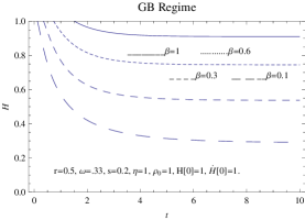
Figure 1: Illustrates $H$ vs. $t$ in GB dominated regime for various $\beta$ with other known parameters.

(ii) The variation of $a$ with $t$ in GB dominated regime for different values of bulk viscous constant $(\beta)$ is plotted in the Fig. 2. It is evident that $a$ has increasing nature characteristics with the cosmic time. It is also found that at a specified moment the higher values of scale factor lead to higher values of bulk viscous constant.

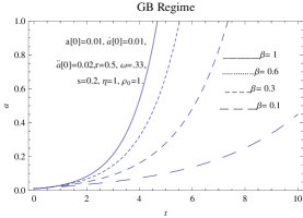
Figure 2: Illustrates $a$ vs. $t$ in GB dominated regime for various $\beta$ with other known parameters.

To study analytic solutions of known form for causal cosmology in GB regime we consider following special cases.

3.1.1 Power-law expansion:

In power-law model, scale factor of the universe evolves as $a(t)=a_{0}t^{D}$, where $a_{0}$ and exponent $D$ indicate constant parameters. In this model, deceleration parameter ($q$) yields $q=\frac{1-D}{D}$, it shows accelerated expansion for $D>1$. In GB regime, the energy density and the viscous stress can be represented as respectively

$$\rho=\rho_{0}D^{3}t^{-3},\;\;\;\;\;\;\Pi=-\rho_{0}D^{2}((1+\omega)D-1)t^{-3},$$ (19)

where exponent $D>\frac{1}{(1+\omega)}$ indicate physically relevant solutions ($\Pi<0$). In GB regime for power-law expansion with Full Israel Stewart (FIS) theory the field Eq. (18) yields

$$A_{1}+A_{2}t^{3r-2}+A_{3}t^{3(r-s)}=0,$$ (20)

where $A_{1}=\frac{3}{2}(r-s+\frac{1}{1+\omega})-\frac{3D}{2}((1+\omega)(r-s)+2)$, $A_{2}=\frac{1}{\beta}\rho_{0}^{1-r}D^{3-3r}(D(1+\omega)-1)$ and $A_{3}=-3\eta\rho_{0}^{s-r}D^{3s-3r+2}$. In GB regime power-law solution is permitted for the subsequent cases:
Case (i) $r\neq\frac{2}{3}$ and $s\neq r$: Power-law solution is permitted for $A_{1}=A_{2}=A_{3}=0$, which yields $\rho_{0}=0$. It shows a physically non realistic power-law solution.
Case (ii) $r\neq\frac{2}{3}$ and $s=r$: Power-law solution is permitted for $A_{1}+A_{3}=0$ and $A_{2}=0$. It gives the power-law exponent $D=\frac{1}{1+\omega}$. It indicates that bulk viscous stress $(\Pi)$ becomes zero, which is not physically acceptable solution.
Case (iii) $r\neq\frac{2}{3}$ and $s=\frac{2}{3}$: In this case, power-law solution is permitted for $A_{1}=0$ and $A_{2}+A_{3}=0$. It yields the bulk viscus constant $\beta_{1}=\frac{(D(1+\omega)-1)\rho_{0}^{\frac{1}{3}}}{3D}$ and the power-law exponent $D=r+\frac{1-2\omega}{3(1+\omega)}$ or $\frac{1}{1+\omega}$. We note that physically viable solution is permitted for $D=r+\frac{1-2\omega}{3(1+\omega)}$. In this type of dissipative process the values of power law exponent $(D)$ depend on both bulk viscous parameter $r$ and parameter of state $(\omega)$. However for $\omega=\frac{1}{2}$, exponent $D$ depends on $r$ particularly. If we choose $r=\frac{5}{3}+\frac{\omega}{1+\omega}$ as a special case, it gives $D=2$. In this special case, the deceleration parameter becomes $q=-0.5$ which leads to current observed values of $q$ [60].
Case (iv) $r=s=\frac{2}{3}$: In this case, power-law evolutions are permitted in GB dominated regime for $A_{1}+A_{2}+A_{3}=0$ which leads to

$$\left[1+\omega+\frac{2(1+\omega)\rho_{0}^{\frac{1}{3}}}{3\beta}-2\eta\right]D^{2}+\left[2+\frac{2\rho_{0}^{\frac{1}{3}}}{3\beta}\right]D+\frac{1}{1+\omega}=0.$$ (21)

Power law type inflation is permitted ($D>>1$) in Full Israel Stewart theory for known values of other parameters used in Eq. (21). Figure 3 illustrates the variation of $D$ vs. $\omega$ for various $\beta$. The shadow region of the Fig. 3 represents $\Pi>0$, which is unsuitable for power law expansion. The figure demonstrates that the power law inflation in GB dominated regime is motivated for higher $\omega$ and higher $\beta$.

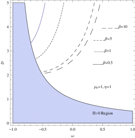
Figure 3: Illustrates $D$ vs $\omega$ in GB regime for various $\beta$ with other known parameters.

In the absence of bulk viscosity ($\beta=\beta_{1}=0$) the field equation ($\dot{H}+(1+\omega)H^{2}=0$) in GB regime yields power law type expansion ($a(t)=a_{0}t^{D}$) unless $\omega=-1$, where power law exponent $D=\frac{1}{(1+\omega)}$. In GB regime without bulk viscosity, power law type accelerated expansion ($D>1$) is permitted for $0>\omega>-1$.

3.1.2 Exponential model :

Exponential type cosmic evolution $(a(t)\sim e^{H_{1}t})$ is permitted in RS brane with GB term for $\ddot{H}=\dot{H}=0$ or $H=const.=H_{1}$ in Eq. (18). Exponential expansion leads de Sitter type expansion for $H_{1}>0$ even in the presence of matters. For exponential expansion type model the Hubble’s parameter in GB regime yields

$$\frac{(1+\omega)}{\beta}\rho_{0}^{1-r}H_{1}^{2-3r}-3\eta\rho_{0}^{s-r}H_{1}^{3(s-r)}+\frac{3(1+\omega)}{2}=0.$$ (22)

Several possibility arises to implement an exponential expansion in GB regime. Subsequent cases are considered for simplicity:
Case (i)$s\neq\frac{2}{3}$ and $r=s$ : In this particular case exponent $(H_{1})$ of exponential expansion reduces to $H_{1}=\left[\frac{3\beta(2\eta-1-\omega)}{2(1+\omega)\rho_{0}^{1-r}}\right]^{\frac{1}{2-3s}}$. The de Sitter type expansion is permitted for $2\eta-1>\omega>-1$. The causality condition ($\omega\leq 1$) of the solution implies following constraint on the upper range of parameter $\eta$, which is $\eta\leq 1$.
Case (ii) $r\neq\frac{2}{3}$ and $s=\frac{2}{3}$ : The exponent $(H_{1})$ of exponential expansion yields $H_{1}=\left[\frac{3(1+\omega)\rho_{0}^{r-\frac{2}{3}}}{2(3\eta-\frac{1+\omega}{\beta}\rho_{0}^{\frac{1}{3}})}\right]^{\frac{1}{2-3r}}$. Exponential expansion is permitted for (i) $\omega>-1$ and $\beta_{1}>\frac{(1+\omega)\rho_{0}^{\frac{1}{3}}}{3\eta}$, (ii) $\omega<-1$ and $\beta_{1}<\frac{(1+\omega)\rho_{0}^{\frac{1}{3}}}{3\eta}$. However, former one represents exponential solution for quintessence like fluid and the later one represents that for phantom like fluid.
Case (iii) $r=\frac{2}{3}$ and $s\neq\frac{2}{3}$ : In this particular case exponent $(H_{1})$ of exponential expansion reduces to $H_{1}=\left[\frac{(1+\omega)\rho_{0}^{\frac{2}{3}}}{3\eta\rho_{0}^{s}}\left(\frac{\rho_{0}^{\frac{1}{3}}}{\beta}+\frac{3}{2}\right)\right]^{\frac{1}{3s-2}}$. Here the de Sitter type expansion is permitted for $\omega>-1$, $\beta>0$ and $\eta>0$.
In the absence of bulk viscosity ($\beta=\beta_{1}=0$) the field equation ($\dot{H}+(1+\omega)H^{2}=0$) in GB regime yield exponential expansion ($a(t)=e^{H_{1}t}$) for $\omega=-1$, which permits accelerated expansion for $H_{1}>0$.
We now study stability of the cosmic evolution in the GB dominated regime with causal dissipation. The exponential evolution admits accelerating phase for $H_{1}>0$. In the causal cosmology the cosmological evolution is directed by differential equation which is second order in nature. To revise stability of cosmic evolution due to equilibrium points or fixed points in GB dominated regime, one can rewrite Eq. (18) in term of two autonomous first order differential equations which are

$$\dot{H}=y,$$

$$\dot{y}=P(y,H)=-\frac{3}{2}\left[r-s-\frac{1+4\omega}{3(1+\omega)}\right]\frac{y^{2}}{H}-\left[\frac{3}{2}(1+\omega)(r-s)+3+\frac{\rho_{0}^{1-r}}{\beta}H^{2-3r}\right]Hy$$

$$-\left[\frac{1+\omega}{\beta}\rho_{0}^{1-r}H^{5-3r}-3\eta\rho_{0}^{s-r}H^{3(s-r+1)}+\frac{3}{2}(1+\omega)H^{3}\right].$$ (23)

The phase point $P(0,H_{1})=0$ or the equilibrium point is described by $\dot{y}=y=0$ in Eq. (23). Considering the expansion of Taylor’s and linear approximation [61] about the fixed points, the Eq. (23) becomes

$$\dot{y}=e\;H+h\;y\;.$$ (24)

Where the constants are given by $e=-(1+\omega)H_{1}^{2}\left[\frac{2-3s}{\beta}\rho_{0}^{1-r}H_{1}^{2-3s}+\frac{9}{2}(r-s)\right]$ and $h=-H_{1}\left[\frac{3}{2}(1+\omega)(r-s)+3+\frac{1}{\beta}\rho_{0}^{1-r}H_{1}^{2-3r}\right]$. The equilibrium points associate to the de Sitter type evolution in GB dominated regime are characterized in Table 1. The exponential expansions corresponding stable acceleration are realized by (i) $r\geq s$, $s<\frac{2}{3}$, $2\eta-1\geq\omega>-1$ and $0<\eta\leq 1$ (ii) $r>s$, $s\leq\frac{2}{3}$, $2\eta-1\geq\omega>-1$ and $0<\eta\leq 1$.

Stability of fixed points associated to de Sitter type expansion in GB dominated regime for causal solution. $Constraints\;of\;parameters$ $Type\;of\;equilibrium\;points$ $r\geq s$, $s<\frac{2}{3}$, $2\eta-1\geq\omega>-1$, and $0<\eta\leq 1$ $stable\;attractor$ $r>s$, $s\leq\frac{2}{3}$, $2\eta-1\geq\omega>-1$ and $0<\eta\leq 1$ $stable\;attractor$ $r<s$, $s\geq\frac{2}{3}$, $\omega>-1$ and $H_{1}>0$ $unstable\;saddle$ $r=s$, $s=\frac{2}{3}$ and $H_{1}>0$ $centre$ $r<s$, $s<\frac{2}{3}$, $\omega>-1$, $H_{1}>\left[\frac{9(s-r)\beta}{2\rho_{0}^{1-r}}\right]^{\frac{1}{2-3s}}$ $stable\;attractor$

3.1.3 Evolution in the vicinity of the stationary solution :

In Eq. (22) $H=H_{1}$ implies exponential inflationary expansion in GB regime with a constant rate given by $H_{1}$. We want to examine analytically in detail the behaviour of both Hubble parameter ($H$) and scale factor $(a(t))$ when cosmological evolution is close to any stationary solution $(H_{1})$. The behaviour of the Hubble parameter in vicinity of stationary solutions are studied by setting $H=H_{1}+\chi$ and $\chi<<H_{1}$. Using the relation the behaviour of scale factor in the vicinity of stationary solution yields $a(t)=a_{0}^{\prime}e^{H_{1}t+\int\chi dt}$, where $a_{0}^{\prime}$ is a constant parameter. By Setting $H=H_{1}+\chi$, with $|\chi<<H_{1}|$ and after linearization Eq.(18) yields,

$$\ddot{\chi}+\lambda_{1}\dot{\chi}+\lambda_{2}\chi=0,$$ (25)

where we consider the constant parameters $\lambda_{1}=(\frac{7+4\omega}{2}+\frac{H_{1}^{2-3r}}{\beta\rho_{0}^{r-1}})H_{1}$, $\lambda_{2}=(\frac{(1+\omega)(2-3s)}{\beta\rho_{0}^{r-1}}H_{1}^{2-3r}+\frac{3(1+4\omega)}{2})H_{1}^{2}$ and $r-s-\frac{1+4\omega}{3(1+\omega)}=0$. The solution of above Eq. (25) yields

$$\chi(t)=\chi_{1}e^{\delta_{+}t}+\chi_{2}e^{\delta_{-}t},$$ (26)

where $\chi_{1}$ and $\chi_{2}$ are constants which depend on initial conditions. Here $\delta_{+}$ and $\delta_{-}$ are the roots satisfying following relation

$$\delta_{\pm}=\frac{\lambda_{1}}{2}\left[-1\pm\sqrt{1-\frac{4\lambda_{2}}{\lambda_{1}^{2}}}\right].$$ (27)

Several possibilities arise and following cases are consider for simplicity:
Case (i) weak damping $(\lambda_{1}^{2}<4\lambda_{2})$ : The quantity below square root in Eq. (27) turns into negative and the corresponding solution for $\chi$ yields $\chi(t)=\chi(0)e^{-\frac{\lambda_{1}t}{2}}cos(\frac{1}{2}\sqrt{\lambda_{1}^{2}-4\lambda_{2}}\;t)$, where $\chi(0)$ is an initial value constant. Hence Hubble parameter ($H$) exhibits an oscillatory damped behaviour of frequency $n=\frac{1}{2}\sqrt{\lambda_{1}^{2}-4\lambda_{2}}$ around the stationary solution $(H=H_{1})$. The damped oscillatory solution yields inflation with oscillation given by the term $\int\chi dt={e^{-\frac{\lambda_{1}t}{2}}[a_{1}cos(\frac{1}{2}\sqrt{\lambda_{1}^{2}-4\lambda_{2}}\;t+a_{2}sin(\frac{1}{2}\sqrt{\lambda_{1}^{2}-4\lambda_{2}}\;t]}$, where $a_{1},\;a_{2}$ are constants. This nearly stationary solution has the curious feature [62]. In GB regime for $r=\frac{2}{3}$, one can obtain a damped oscillatory behaviour around $H_{1}$ for the constraint $\frac{\rho_{0}^{\frac{1}{3}}}{\beta}<\frac{12\omega-3}{2}\pm 2\sqrt{8\omega^{2}-2\omega-1}$. To show stable evolution in the vicinity of the stationary solution, one can plot $H$ versus $t$ for $|\chi<<H_{1}|$. Here the solution will be a stable spiral for $s\leq\frac{2}{3}$ and $\omega>-\frac{1}{4}$. Figure 4 shows $H$ vs. $t$ for a specified other parameters in GB regime. The figure shows stable expansion of the universe with time around a equilibrium point $(H_{1})$ for different values of $\chi$ ( $<<H_{1}$), $\lambda_{1}^{2}<4\lambda_{2}$ and $\lambda_{1}>0$.

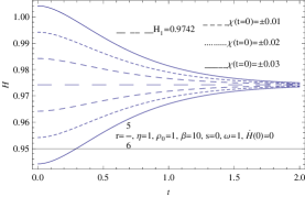
Figure 4: Illustrates $H$ vs $t$ in GB dominated regime for various $\chi(t=0)$ with a known set of parameters.

Case (ii) strong damping $(\lambda_{1}^{2}>4\lambda_{2})$ : The quantity below square root in Eq. (27) is real and both roots in Eq. (27) shall be real. Furthermore, the quantity within the square bracket in Eq. (27) is negative for $\lambda_{2}>0$. Hence both solutions shall be a stable node for $s\leq\frac{2}{3}$ and $\omega>-\frac{1}{4}$. The solution yields inflation with the term $\int\chi dt=a_{1}^{\prime}e^{\delta_{+}t}+a_{2}^{\prime}e^{\delta_{-}t}$, where $a_{1}^{\prime}$ and $a_{2}^{\prime}$ are constants.
Case (iii) critical damping $(\lambda_{1}^{2}=4\lambda_{2})$ : In this case $\delta_{+}=\delta_{-}=-\frac{\lambda_{1}}{2}$, the solutions are given by $\chi(t)=\left(a_{1}^{{}^{\prime\prime}}+a_{2}^{{}^{\prime\prime}}t\right)e^{-\frac{\lambda_{1}t}{2}}$, where $a_{1}^{{}^{\prime\prime}}$ and $a_{2}^{{}^{\prime\prime}}$ are constants. The solutions resemble those for strong damping and the solutions show a stable node for $s\leq\frac{2}{3}$ and $\omega>-\frac{1}{4}$.
Case (iv) $\lambda_{2}<0$: In this case $\delta_{+}$ and $\delta_{-}$ are real but opposite sign. The solutions show a unstable saddle for (i) $s\geq\frac{2}{3}$ and $-\frac{1}{4}>\omega>-1$, (ii) $s\leq\frac{2}{3}$ and $\omega<-1$.
In the absence of bulk viscosity ($\beta=\beta_{1}=0$) the field equation in GB regime yields $\dot{H}+(1+\omega)H^{2}=0$ which is a first order differential equation of $H$. In the absence of bulk viscosity damped oscillatory behaviour of Hubble parameter ($H$) in the vicinity of stationary solution ($H_{1}$) is not permitted due to the order of the field equation.

3.2 RS dominated regime:

Field equation in braneworld gravity (RS II) with FIS theory is obtained from Eq. (12) by setting $\epsilon=1$, which yields

$$\ddot{H}+\frac{1}{2}\left[r-s-\frac{3+4\omega}{(1+\omega)}\right]\frac{\dot{H^{2}}}{H}+\left[\frac{3}{2}(1+\omega)(r-s)+3+\frac{\rho_{0}^{1-r}}{\beta}H^{-r}\right]H\dot{H}$$

$$+3H^{3}\left[\frac{(1+\omega)}{\beta}\rho_{0}^{1-r}H^{-r}-3\eta\rho_{0}^{s-r}H^{(s-r)}+\frac{3}{2}(1+\omega)\right]=0.$$ (28)

The field Eq. (28) is very non linear to acquire a wide-ranging analytical solution in RS regime. Though, we can study relevant numerical solutions of cosmological parameters for instance Hubble parameter $(H)$, scale factor $(a)$. We study numerically the evolution of the universe as follows:
(i) The variation of $H$ with $t$ in RS dominated regime for different values of bulk viscous constant $(\beta)$ is plotted in the Fig. 5. It shows that the evolution of $H$ has declining nature characteristics with cosmic time. It is found that at a specified moment the smaller values of $H$ lead to smaller values of bulk viscous constant.

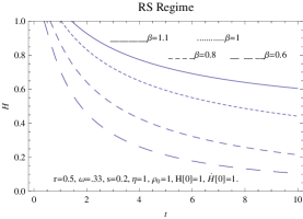
Figure 5: Illustrates $H$ vs. $t$ in RS dominated regime for various $\beta$ with other known parameters.

(ii) The variation of $a$ with $t$ in RS dominated regime for different values of bulk viscous constant $(\beta)$ is plotted in the Fig. 6. It is evident that $a$ has increasing nature characteristics with the cosmic time. It is also found that at a specified moment the higher values of scale factor lead to higher values of bulk viscous constant.

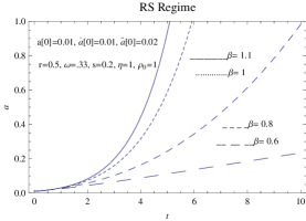
Figure 6: Illustrates $a$ vs. $t$ in RS dominated regime for various $\beta$ with other known parameters.

To study analytic solution of known form for causal cosmology in RS regime we consider following special cases.

3.2.1 Power-law expansion :

In power-law model the evolution of the scale factor of the universe yields $a(t)=a_{0}t^{D}$, where $a_{0}$ and $D$ are constant parameter. In RS regime with power-law expansion, the expression of density of energy and bulk viscous pressure yield, respectively

$$\rho=\rho_{0}Dt^{-1},\;\;\;\;\;\;\Pi=-\rho_{0}[(1+\omega)D-\frac{1}{3}]t^{-1},$$ (29)

where $D>\frac{1}{3(1+\omega)}$ for physically relevant solutions ($\Pi<0$). In RS regime for power-law expansion with Full Israel Stewart (FIS) theory, the field Eq. (28) yields

$$B_{1}+B_{2}t^{r}+B_{3}t^{(r-s)}=0,$$ (30)

where $B_{1}=\frac{9}{2}(1+\omega)D^{2}-\frac{3D}{2}((1+\omega)(r-s)+2)+\frac{1}{2}(r-s)+\frac{1}{2(1+\omega)}$, $B_{2}=\frac{1}{\beta}\rho_{0}^{1-r}D^{1-r}[3(1+\omega)D-1]$ and $B_{3}=-9\eta\rho_{0}^{s-r}D^{s-r+2}$. In RS regime power-law solutions are permitted in the following cases:
Case (i) $r\neq 0$ and $s\neq r$: Power-law solution is permitted for $B_{1}=B_{2}=B_{3}=0$. It shows $\rho_{0}=0$ which is not physically accepted solution.
Case (ii) $r\neq 0$ and $s=r$: In this case, power-law solution is permitted for $B_{1}+B_{3}=0$ and $B_{2}=0$. It shows the power-law exponent $D=\frac{1}{3(1+\omega)}$. It indicates that the value of bulk viscous stress $(\Pi)$ become zero, which is also not physically acceptable power-law solution.
Case (iii) $r\neq 0$ and $s=0$: In this case, power-law solutions are permitted for $B_{1}=0$ and $B_{2}+B_{3}=0$. It shows the bulk viscus constant $\beta_{1}=\frac{(3(1+\omega)D-1)\rho_{0}}{9D}$ and the power-law exponent $D=\frac{r}{3}+\frac{1}{3(1+\omega)}$ or $\frac{1}{3(1+\omega)}$. Here we note that physically viable solution are permitted for $D=\frac{r}{3}+\frac{1}{3(1+\omega)}$. At this particular situation the values power law exponent $(D)$ depends on bulk viscous parameter $r$ and equation of state parameter $(\omega)$. If we choose $r=5+\frac{\omega}{1+\omega}$ as a special case, it yields power-law exponent $D=2$. Hence, the deceleration parameter $(q)$ becomes $q=-0.5$. In this context, One could note that the present value of deceleration parameter $(q)$ is very closed to $q\sim-0.5$.
Case (iv) $r=s=0$: In this case, power-law evolutions are acquired in the RS dominated regime and FIS theory for $B_{1}+B_{2}+B_{3}=0$ which leads to

$$9\left[1+\omega-2\eta+\frac{2(1+\omega)\rho_{0}}{3\beta}\right]D^{2}-2\left[3+\frac{\rho_{0}}{\beta}\right]D+\frac{1}{1+\omega}=0.$$ (31)

The power-law dominated inflation is permitted in Full Israel Stewart theory with known values of other parameters in Eq. (31). Figure 7 shows the variation of $D$ vs. $\omega$ for various $\beta$. Shadow section of Fig. 7 represents physically unsuitable ($\Pi>0$) region in power law type evolution. The figure suggests that high values of $\omega$ and $\beta$ are appropriate for power law inflation in RS dominated regime.

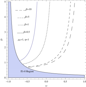
Figure 7: Illustrates $D$ vs $\omega$ in RS dominated regime for various $\beta$ with other known parameters.

In the absence of bulk viscosity ($\beta=\beta_{1}=0$) the field equation ($\dot{H}+3(1+\omega)H^{2}=0$) in RS regime yields power law type expansion ($a(t)=a_{0}t^{D}$) unless $\omega=-1$, where power law exponent $D=\frac{1}{3(1+\omega)}$. In RS regime without bulk viscosity, power law type accelerated expansion ($D>1$) is permitted for $-\frac{2}{3}>\omega>-1$.

3.2.2 Exponential expansion:

Exponential type cosmic model $(a(t)\sim e^{H_{1}t})$ is permitted in RS brane for $\ddot{H}=\dot{H}=0$ or $H=const.=H_{1}$ of Eq. (28). Exponential expansion leads to de Sitter type expansion for $H_{1}>0$ even in the presence of matters. In exponential expansion model the Hubble’s parameter in RS region yields

$$\frac{(1+\omega)}{3\beta}\rho_{0}^{1-r}H_{1}^{-r}-\eta\rho_{0}^{s-r}H_{1}^{s-r}+\frac{(1+\omega)}{2}=0.$$ (32)

In RS regime for exponential expansion, following cases for simplicity are studied:
Case (i) $r=s$ and $s\neq 0$ : The exponent $(H_{1})$ of exponential expansion yields $H_{1}=\left[\frac{3\beta(2\eta-1-\omega)}{2(1+\omega)\rho_{0}^{1-r}}\right]^{-\frac{1}{s}}$. The de Sitter type expansion is permitted for $2\eta-1>\omega>-1$. The causality ($\omega\leq 1$) of the solution implies following constraint on the parameter $\eta$, which is $0<\eta\leq 1$.
Case (ii) $r\neq 0$ and $s=0$ : In this case, exponential exponent $(H_{1})$ yields $H_{1}=\left[\frac{3(1+\omega)\rho_{0}^{r}}{2(3\eta-\frac{1+\omega}{\beta}\rho_{0})}\right]^{-\frac{1}{r}}$. Here exponential expansion is permitted for the following constraint among the parameters $1\geq\omega>-1$ and $\beta_{1}>\frac{(1+\omega)\rho_{0}}{3\eta}$.
Case (iii) $r=0$ and $s\neq 0$ : In this particular case exponent $(H_{1})$ of exponential expansion reduces to $H_{1}=\left[\frac{(1+\omega)}{3\eta\rho_{0}^{s}}\left(\frac{\rho_{0}}{\beta}+\frac{3}{2}\right)\right]^{\frac{1}{s}}$. In RS regime, de Sitter type expansion is permitted here for $1\geq\omega>-1$, $\eta>0$ and $\beta>0$.
In the absence of bulk viscosity ($\beta=\beta_{1}=0$) the field equation ($\dot{H}+3(1+\omega)H^{2}=0$) in RS regime yield exponential expansion ($a(t)=e^{H_{1}t}$) for $\omega=-1$, which permit exponential accelerated expansion for $H_{1}>0$.
Adopting the method for stability analysis of GB dominated regime, it is also possible to learn stability for the evolution in the RS dominated regime with dissipative effect. The exponential evolution admits accelerating phase for $H_{1}>0$. To revise stability of cosmic evolution due to equilibrium points or fixed points in RS dominated regime with causal theory, one can rewrite Eq. (28) in term of two autonomous first order differential equations which are

$$\dot{H}=y,$$

$$\dot{y}=P(y,H)=-\frac{1}{2}\left[r-s-\frac{3+4\omega}{1+\omega}\right]\frac{y^{2}}{H}-\left[\frac{3}{2}(1+\omega)(r-s)+3+\frac{\rho_{0}^{1-r}}{\beta}H^{-r}\right]Hy$$

$$-3\left[\frac{1+\omega}{\beta}\rho_{0}^{1-r}H^{3-3r}-3\eta\rho_{0}^{s-r}H^{s-r+3}+\frac{3}{2}(1+\omega)H^{3}\right].$$ (33)

The phase points $P(0,H_{1})=0$ in phase space are distinguished by $\dot{y}=y=0$. Following expansion of Taylor’s series and linear approximation [61] of fixed points, Eq. (28) becomes

$$\dot{y}=e^{\prime}H+h^{\prime}y\;,$$ (34)

where the constants $e^{\prime}=-3(1+\omega)H_{1}^{2}\left[\frac{(-s)}{\beta}\rho_{0}^{1-r}H_{1}^{-s}+\frac{3}{2}(r-s)\right]$ and $h^{\prime}=-H_{1}\left[\frac{3}{2}(1+\omega)(r-s)+3+\frac{1}{\beta}\rho_{0}^{1-r}H_{1}^{-r}\right]$. The characteristics of fixed points associate to de Sitter type evolution in RS dominated regime are exposed within Table 2. Stable accelerated exponential evolution is permitted for (i) $r\geq s$, $s<0$, $2\eta-1\geq\omega>-1$ and $0<\eta\leq 1$ (ii) $r>s$, $s\leq 0$, $2\eta-1\geq\omega>-1$ and $0<\eta\leq 1$.

Stability of fixed points associated to de Sitter type expansion in RS dominated regime for causal solution. $Constraints\;of\;parameters$ $Type\;of\;equilibrium\;points$ $r\geq s$, $s<0$, $2\eta-1\geq\omega>-1$, and $0<\eta\leq 1$ $stable\;attractor$ $r>s$, $s\leq 0$, $2\eta-1\geq\omega>-1$ and $0<\eta\leq 1$ $stable\;attractor$ $r<s$, $s\geq 0$, $\omega>-1$ and $H_{1}>0$ $unstable\;saddle$ $r=s$, $s=0$ and $H_{1}>0$ $centre$ $r<s$, $s<0$, $\omega>-1$, $H_{1}>\left[\frac{3(s-r)\beta}{2\rho_{0}^{1-r}}\right]^{\frac{-1}{r}}$ $stable\;attractor$

3.2.3 Evolution in the vicinity of the stationary solution :

In Eq. (32) $H=H_{1}$ implies inflationary expansion with a constant rate given by $H_{1}$. To examine the behaviour of the scale factor and the Hubble parameter in the vicinity of the stationary solution analytically, one can consider the perturbation as $H=H_{1}+\chi$ and $\chi<<H_{1}$. Using the relation the analytic behaviour of scale factor in the vicinity of stationary solution yields $a(t)=a_{0}e^{H_{1}t+\int\chi dt}$. By Setting $H=H_{1}+\chi$, with $|\chi<<H_{1}|$ and after linearization Eq.(28) yields,

$$\ddot{\chi}+\lambda_{3}\dot{\chi}+\lambda_{4}\chi=0,$$ (35)

where we consider the constants $\lambda_{3}=(\frac{15+12\omega}{2}+\frac{H_{1}^{-r}}{\beta\rho_{0}^{r-1}})H_{1}$, $\lambda_{4}=3(\frac{(1+\omega)(-s)}{\beta\rho_{0}^{r-1}}H_{1}^{-r}+\frac{3(3+4\omega)}{2})H_{1}^{2}$ and $r-s-\frac{3+4\omega}{(1+\omega)}=0$. The solution of above Eq. (35) yields

$$\chi(t)=\chi_{3}e^{\delta^{\prime}_{+}t}+\chi_{4}e^{\delta^{\prime}_{-}t},$$ (36)

where $\chi_{3}$ and $\chi_{4}$ are constants which depend on initial conditions. Here $\delta^{\prime}_{+}$ and $\delta^{\prime}_{-}$ are the roots satisfying following relation

$$\delta^{\prime}_{\pm}=\frac{\lambda_{3}}{2}\left[-1\pm\sqrt{1-\frac{4\lambda_{4}}{\lambda_{3}^{2}}}\right].$$ (37)

Several possibilities arise and following cases are consider for simplicity:
Case (i) weak damping $(\lambda_{3}^{2}<4\lambda_{4})$ : The quantity within the square root in Eq. (37) will be negative and the corresponding solution for $\chi$ yields $\chi(t)=\chi^{\prime}(0)e^{-\frac{\lambda_{3}t}{2}}cos(\frac{1}{2}\sqrt{\lambda_{3}^{2}-4\lambda_{4}}\;t)$ , where $\chi^{\prime}(0)$ is a constant. Hence Hubble parameter ($H$) exhibits an oscillatory damped behaviour of frequency $n=\frac{1}{2}\sqrt{\lambda_{3}^{2}-4\lambda_{4}}$ around the stationary solution $(H=H_{1})$. The damped oscillatory solution yields inflation with oscillation given by the term $\int\chi dt={e^{-\frac{\lambda_{3}t}{2}}[b_{1}cos(\frac{1}{2}\sqrt{\lambda_{3}^{2}-4\lambda_{4}}\;t+b_{2}sin(\frac{1}{2}\sqrt{\lambda_{3}^{2}-4\lambda_{4}}\;t]}$, where $b_{1}$ and $b_{2}$ are constants. This nearly stationary solution has the curious feature [62]. Stable expansion of the universe with time around a equilibrium points $(H_{1})$ are permitted for $\lambda_{3}^{2}<4\lambda_{4}$ and $\lambda_{3}>0$. Hence the solution will be stable spiral for $s\leq 0$ and $\omega>-\frac{3}{4}$. In RS regime for $r=0$, one can obtain a damped oscillatory behaviour around $H_{1}$ for the constraint among the parameters $\frac{\rho_{0}}{\beta}<\frac{21+36\omega}{2}\pm 6\sqrt{8\omega^{2}+10\omega+3}$.
Case (ii) strong damping $(\lambda_{3}^{2}>4\lambda_{4})$ : The quantity within the square root in Eq. (37) is real and both roots in Eq. (36) will be real. Furthermore, the quantity within the square bracket in Eq. (37) is negative for $\lambda_{4}>0$. Hence both solutions shall be stable node for $s\leq 0$ and $\omega>-\frac{3}{4}$. The solution yields inflation with the term $\int\chi dt=b_{1}^{\prime}e^{\delta^{\prime}_{+}t}+b_{2}^{\prime}e^{\delta^{\prime}_{-}t}$.

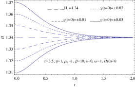
Figure 8: Illustrates $H$ vs. $t$ in RS dominated regime for various $\chi(t=0)$ for a known set of parameters.

To examine stable expansion in the vicinity of the stationary solution, one can plot $H$ vs. $t$ for various $\chi$ ($<<H_{1}$). Figure 8 shows $H$ vs. $t$ for a given value of other parameters in RS regime. The figure shows stable expansion in the vicinity of stationary solution $(H_{1})$ for $\lambda_{3}^{2}>4\lambda_{4}$ and $\lambda_{4}>0$.
Case (iii) critical damping $(\lambda_{3}^{2}=4\lambda_{4})$ : In this case $\delta^{\prime}_{+}=\delta^{\prime}_{-}=-\frac{\lambda_{3}}{2}$, the solutions yield $\chi(t)=\left(b_{1}^{{}^{\prime\prime}}+b_{2}^{{}^{\prime\prime}}t\right)e^{-\frac{\lambda_{3}t}{2}}$, here $b_{1}^{{}^{\prime\prime}}$, $b_{2}^{{}^{\prime\prime}}$ stand for arbitrary constants. The solutions resemble those for strong damping and the solutions show a stable node for $s\leq 0$ and $\omega>-\frac{3}{4}$.
Case (iv) $\lambda_{4}<0$: In this case $\delta^{\prime}_{+}$ and $\delta^{\prime}_{-}$ are real but opposite sign. The solutions show a unstable saddle for (i) $s\geq 0$ and $-\frac{3}{4}>\omega>-1$, (ii) $s\leq 0$ and $\omega<-1$.
In the absence of bulk viscosity ($\beta=\beta_{1}=0$) the field equation in RS regime yields $\dot{H}+3(1+\omega)H^{2}=0$ which is a first order differential equation of $H$. In the absence of bulk viscosity damped oscillatory behaviour of Hubble parameter ($H$) in the vicinity of stationary solution ($H_{1}$) is not permitted for the order of the field equation.

4 Discussion

In the article, we investigate causal cosmological solutions for RS braneworld theory with Gauss-Bonnet (GB) coupling. Here we consider the total effective cosmic pressure $(p_{eff})$ contains two part, namely, isotropic pressure ($p$) part along with bulk viscous pressure ($\Pi$) part. The isotropic part of fluid ($p$) is explained by a EoS which yields $p=\omega\rho$, where $\rho$ is the energy density and $\omega$ is EoS parameter. The bulk viscous stress ($\Pi$) is explained by a causal theory, namely, Full Israel Stewart (FIS). In the causal cosmology the relaxation time and bulk viscous coefficient are expressed by respectively $\tau=\beta\rho^{r-1}$ and $\zeta=\beta_{1}\rho^{s}$, where $\beta(\geq 0),\;\beta_{1}(\geq 0),\;s(\geq 0)$ and $r(\geq 0)$ are constant parameters. The field equations that govern causal cosmological solutions in GB and RS regime are very nonlinear for find an universal analytical solution. For acquiring analytic solutions of causal cosmology in GB and RS regime we consider following cases. Case (1) $r=s=\frac{\epsilon-1}{\epsilon}$: The corresponding analytical solutions support cosmic exponential inflation in parametric form of time for GB dominated and RS dominated regime, where $\epsilon=3$ and $\epsilon=1$ are in GB and RS regime respectively. Case (ii) $r=\frac{\epsilon-1}{\epsilon}$ and $s=\frac{\epsilon-3}{\epsilon},\;\frac{\epsilon-2}{\epsilon},\;\frac{\epsilon-1}{\epsilon}$: The corresponding analytic solution permits emergent universe model both in GB and RS regime for some constraints among the parameters $(b_{1},\;b_{2},\;b_{3},\;b_{4})$. We have also studied numerical solutions of cosmological parameters, namely, scale factor $a(t)$ and Hubble redshift parameter $H$ both for GB and RS regime. Numerical solutions in GB and RS regime are discussed respectively in Figs. 1-2 and Figs. 5-6 for a given set of parameters. The Figs. 1 and 5 propose a declining nature of Hubble parametric ($H$) function with evolution ($t$). Figures 2 and 6 suggest that scale factor $a(t)$ is growing function among time $(t)$. The figures show that in GB regime the universe evolve more rapidly than RS regime and for a particular time, the values of scale factor are bigger with higher magnitudes of bulk viscous constant ($\beta$). Analytic solutions of known from such as Power-law expansion, Exponential model and evolution in the vicinity of stationary solution are also discussed for GB dominated and RS dominated regime. Power-law solution $(a\sim t^{D})$ is permitted with $s=\frac{2}{3}$ and $s=0$ in GB and RS regime respectively. Figures (3) and (7) show plot of power law exponent ($D$) versus EoS parameter ($\omega$) with different bulk viscous parameter ($\beta$). The figures suggest that the opportunity for Power-law acceleration increases with larger $\omega$ and $\beta$ both for GB and RS regime. Exponential evolution is permitted for GB dominated era and RS dominated era. The results of stability of fixed points with causal viscosity are summarized within Table 1 and Table 2 for GB and RS regime respectively. Exponential type stable expansion is acquired for (i) $r\geq s$ , $s<\frac{2}{3}$ and $1\geq\omega>-1$ (ii) $r>s$ , $s\leq\frac{2}{3}$ and $1\geq\omega>-1$ in GB regime. For RS dominated era, stable exponential expansion is permitted for $r<s$ , $s\leq 0$ and $1\geq\omega>-1$. We also analytically discuss cosmic evolution in the vicinity of the stationary solution. It is found that damped oscillatory behaviour of the Hubble parameter is permitted for causal theory (FIS) both in GB and RS regime. Figures 4 and 8 show respectively $H$ versus $t$ for given other parameters with GB dominated and RS dominated regime. The figures shows stable expansion of the universe with time around a stationary solution $(H_{1})$ for different values of $\chi$ where $|\chi<<H_{1}|$. Stable evolution in the vicinity of the stationary solution is permitted for $s\leq\frac{2}{3},\;\omega>-\frac{1}{4}$,$\;r=s+\frac{1+4\omega}{3(1+\omega)}$ and $s\leq 0,\;\omega>-\frac{3}{4}$, $\;r=s+\frac{3+4\omega}{(1+\omega)}$ respectively in GB and RS regime.
However, in the absence of bulk viscosity ($\Pi=0$), power law type accelerated expansion $(D>1)$ is permitted for $0>\omega>-1$ and $-\frac{2}{3}>\omega>-1$ in GB regime and RS regime respectively. The presence of bulk viscosity ($\Pi\neq 0$) may have several permitted range of $\omega$ for which power law type accelerated expansion is allowed for different values of $\tau$ and $\zeta$ in GB regime and RS regime. Again, in the absence of bulk viscosity exponential expansion is permitted only for $\omega=-1$ in GB regime and RS regime. While the presence of bulk viscosity may have several permitted values of $\omega$ for which exponential expansion is permitted for different values of $\tau$ and $\zeta$ in GB regime and RS regime.
In conclusion, it is shown that damped oscillatory behaviour of the Hubble parameter is permitted in the vicinity of the stationary solution for Full Israel Stewart (FIS) theory both in GB and RS regime. It is also observed that stable stationary solutions are permitted in GB regime for (i) $r\geq s$ , $s<\frac{2}{3}$ and $1\geq\omega>-\frac{1}{4}$ (ii) $r>s$ , $s\leq\frac{2}{3}$ and $1\geq\omega>-\frac{1}{4}$ and that in RS regime for $r<s$ , $s\leq 0$ and $1\geq\omega>-\frac{3}{4}$. Causal cosmology in RS brane including GB term allows Power-law type acceleration with higher equation of state parameter ($\omega$) as well as bulk viscous constant $(\beta)$. We also note down, the incorporation of Gauss Bonnet coupling in the Randall-Sundrum brane-world tends to enhance the cosmic evolution. In this context, we would like to mention that Power-law and Exponential models are permitted in GB and RS regime both in the presence and absence of viscosity. However, due to incorporation of causal viscosity in GB and RS regime, one can also obtain damped oscillatory behaviours of Hubble parameter in the vicinity of stationary solution.

References

- [1] A. G. Riess et. al., Astrophys. J. , 665 (2004).
- [2] T. Padmanabhan, Phys. Rept. , 235 (2003).
- [3] A. A. Starobinsky, JETP Lett. , 682 (1979).
- [4] A. A. Starobinsky, Phys. Letts. B , 99 (1980).
- [5] A. Guth, Phys. Rev. D , 347 (1981).
- [6] P. A. R. Ade, et al., Astron. & Astrophys. 594, A 20 (2016). [ arXiv: 1502.02114].
- [7] S. Capozziello and M. De Laurentis, Phys. Rep. 509, 167 (2011).
- [8] S. Nojiri, & S. D. Odintsov, Int. J. Geom. Meth. Mod. Phys. , 115 (2007).
- [9] S. Nojiri, & S. D. Odintsov, Physics Letters B , 1 (2005).
- [10] E. Elizalde, S. D. Odintsov, E. O. Pozdeeva, S. Yu. Vernov, Int. J. Geom. Meth. Mod. Phys. , 1850188 (2018).
- [11] Y.-F. Cai, S.-H. Chen, J. B. Dent, S. Dutta, & E. N. Saridakis, Class. Quantum Grav. , 215011 (2011).
- [12] K. Bamba, C.-Q. Geng, C.-C. Lee, & L.-W. Luo, J. Cosmol. Astropart. Phys. , 021 (2011).
- [13] S. Capozziello, C. A. Mantica, L. G. Molinari, Int. J. Geom. Meth. Mod. Phys. 16, 1950008 (2019).
- [14] S. Nojiri, S. D. Odintsov, D. Saez-Gomez, Phys. Lett. B , 74 (2009).
- [15] T. Harko, F. S. N. Lobo, S. Nojiri, S. D. Odintsov, Phys. Rev. D , 024020 (2011).
- [16] R. K. Tiwari and A. Beesham, Astrophys. Space Sci. 363, 234 (2018).
- [17] P. S. Debnath, Int. J. Geom. Meth. Mod. Phys. 16, 1950085 (2019).
- [18] T. Nishioka, Class. Quantum Grav. , 242001 (2009).
- [19] C. Ranjit, P. Rudra, Int. J. Theor. Phys. , 636 (2015).
- [20] E. Witten, Nucl. Phys. B 443, 85 (1995).
- [21] P. Horava and E. Witten, Nucl. Phys. B 460, 506 (1996).
- [22] P. Horava and E. Witten, Nucl. Phys. B 475, 94 (1996).
- [23] L. Randall and R. Sundrum, Phys. Rev. Lett. 83, 3370 (1999).
- [24] C-M. Chen, T. Harko, M. K. Mark, Phys. Rev. D 64, 124017 (2001).
- [25] L. Randall and R Sundrum, Phys. Rev. Lett. 83, 4690 (1999).
- [26] J. Maldacena, Adv. Theor. Math. Phys. , 231(1998).
- [27] E. Witten, Adv. Theor. Math. Phys. , 505 (1998).
- [28] S. W. Hawking , T Hertog and H Reall,Phys. Rev. D 62, 043501 (2000).
- [29] S. Nojiri, S. D. Odintsov and S. Zerbini, Phys. Rev. D 62, 064006 (2000).
- [30] M. T. Meehan and I. B. Whittingham JCAP 12 034 (2014).
- [31] S. Nojiri, S. D. Odintsov and S. Ogushi, Int. J. Mod. Phys. A 16, 5085 (2001).
- [32] N. H. Barth and S. M. Christensen, Phys. Rev. D 28, 1876 (1983).
- [33] G. Calcagni , B. de carlos and A. De Felice, Nucl. Phys. B 752, 404 (2006).
- [34] S. S. da Costa, F. V. Roig, J. S. Alcaniz, S. Capozziello, M. De Laurentis and M. Benetti, Class. Quant. Grav. , 075013 (2018).
- [35] S. Chakraborty and T. Bandyopadhyay, Mod. Phys. Lett. A 24, 1915 (2009).
- [36] B. Zweibach, Phys. Lett. B 156, 315 (1985).
- [37] D. Lovelock, J. Math. Phys. 12, 498 (1971).
- [38] N. E. Mavromatos and J. Rizos, Phys. Rev. D 62, 124004 (2000).
- [39] I. P. Neupane, J. High Energy Phys. 09, 040 (2000). [arXiv: hep-th/0008190].
- [40] R.-G. Cai, Z.-K. Guo, S.-J. Wang, Phys. Rev. D , 063514 (2015).
- [41] P. S. Debnath, A. Beesham, B. C. Paul, Class. Quantum Grav. 115010 (2018).
- [42] M. De Laurentis, M. Paolella, and S. Capozziello, Phys. Rev. D , 083531 (2015).
- [43] I. Brevik, E. Elizalde, S. D. Odintsov and A. V. Timoshkin, Int. J. Geom. Meth. Mod. Phys. 14, 1750185 (2017).
- [44] C. W. Misner, The isotropy of the universe, Astrophys. J. 151, 431 (1968).
- [45] J. D. Barrow and R. A. Matzner, Mon. Not. Roy. astron. Soc. 181 , 719 (1977).
- [46] D. Pavon and W. Zimdhal, Phys. Lett. A 179, 261 (1993).
- [47] W. Zimdahl, D. J. Schwarz, A. B. Balakin, D. Pavon, Phys. Rev. D 64, 063501 (2001).
- [48] C. Eckart, Phys. Rev. D , 269 (1940).
- [49] W. Israel, J. M. Stewart, Ann. Phys. 118, 341 (1979).
- [50] M. Cruz, N. Cruz, S. Lepe, Phys. Rev. D 96, 124020 (2017).
- [51] C. Charmousis and J. F. Dufaux, Class. Quant. Grav. 19 , 4671 (2002).
- [52] T. Tsujikawa, M. Sami and R. Maartens, Phys. Rev. D 70, 063525 (2004).
- [53] K. Maeda and T. Torii, Phys. Rev. D 69, 024002 (2004).
- [54] J. E. Lidsey and N. Nunes, Phys. Rev. D 67, 103510 (2003).
- [55] I. Brevik, O. Gorbunova, Eur. Phys. J. C. , 425 (2008).
- [56] P. S. Debnath, B. C. Paul, Mod. Phys. Lett. A 32, 1750216 (2017).
- [57] D. Jou, J. C. Vazquez, G.Lebon, Extended Irreversible Thermodynamics, New York: Spinger (2010).
- [58] S. Mukherjee, B.C. Paul, N. K. Ddhich, S. D. Maharaj and A. Beesham, Classical and Quantum Gravity , 6927 (2006).
- [59] P. S. Debnath, Int. J. Geom. Meth. Mod. Phys. 16, 1950169 (2019).
- [60] P. K. Sahoo, S. K. Tripathy, P. Sahoo, Mod. Phys. Lett. A , 1850193 (2018).
- [61] D. W. Jordan, P. Smith, Nonlinear Ordinary Differential Equations (New York: Oxford 2009).
- [62] D. Pavon, J. B. Bafaluy and D. Jou, Causal Friedmann-Robertson-Walker cosmology, Class. Quant. Grav. (1991) 347.