Lattice Boltzmann Method for wave propagation in elastic solids with a regular lattice: Theoretical analysis and validation

Abstract

The von Neumann stability analysis along with a Chapman-Enskog analysis is proposed for a single-relaxation-time lattice Boltzmann Method (LBM) for wave propagation in isotropic linear elastic solids, using a regular D2Q9 lattice. Different boundary conditions are considered: periodic, free surface, rigid interface. An original absorbing layer model is proposed to prevent spurious wave reflection at domain boundaries. The present method is assessed considering several test cases. First, a spatial Gaussian force modulated in time by a Ricker wavelet is used as a source. Comparisons are made with results obtained using a classical Fourier spectral method. Both P and S waves are shown to be very accurately predicted. The case of Rayleigh surface waves is then addressed to check the accuracy of the method.

1 Introduction

Lattice Boltzman Methods (LBM) are now a popular approach in Computational Fluid Dynamics (e.g. see [1, 2]), with a wide range of applications, ranging from nearly-incompressible flows to multiphase flows, flows in porous media, combustion and recently to supersonic flows, e.g. [3, 4, 5]. They exhibit a very high efficiency when compared to many classical Naviers-Stokes-based solvers, leading to a rapidly growing use for both academic and industrial purposes. Their main advantage comes from their explicit and compact character, along with the use of Cartesian grids. The common feature of Lattice-Boltzmann-like methods is that they rely on the following set of $m$ advection-collision equations:

$$\frac{\partial f_{i}}{\partial t}+\mathbf{c}_{i}\cdot\nabla f_{i}=-\frac{1}{\tau}(M[\mathbf{f}]-f_{i}),\quad i=0,m-1$$ (1)

where the model used for the collision term in the right-hand side is the single relaxation time Bhatnagar-Gross-Krook(BGK) model. Here, $\mathbf{c}_{i}$ is a set of arbitrary solution-independent velocities, $M[\mathbf{f}]$ is a function of $f$ designed to recover the targeted macroscopic equations (the Maxwellian in classical hydrodynamics) and $\tau$ a relaxation time. The computational efficiency of LBM-like approaches comes from the Strang splitting used to decouple the advection and the collision step [6]: the advection step simplifies as a swap in memory without additional floating point operations, while the collision step is strictly local in each cell. The macroscopic quantities such as density, velocity and pressure in fluid mechanics are recovered by post-processing the functions $f_{i}$. A key element in LBM is the choice of the lattice, i.e. the set of $m$ nodes (one per couple $(f_{i},\mathbf{c}_{i})$) needed to solve Eq. (1) at a given node. The dimension $N$ comes from a trade-off between the accuracy, stability and computational efficiency of the method. A lattice is generally denoted $DnQm$, where $n$ and $m$ are the space dimension and the number of nodes in the lattice, respectively.

While LBM originally appeared as a way to solve numerically the Boltzmann equation that statistically describes fluid flow physics, it can also be interpreted and extended as a smart way to solve sets of PDEs, especially for wave propagation [7]. In that case, they must be seen as a purely numerical way to solve an equation, starting from an ad hoc change of variables to recover a set of coupled advection-reaction equations. In order to preserve the efficiency of the method, the advection operator must be linear and the reaction term should be written as a relaxation term. Using this approach, LBM-like methods have been proposed for many physical models, e.g. the heat conduction equation (e.g. [8]), the Schrödinger equation (e.g. [9]) and Maxwell’s equations (e.g. [10, 11]).

The present paper addresses the issue of developing a LBM-like method for the propagation of waves in elastic solids. Up to now, extension of LBM for solid mechanics has been addressed by a very few authors only, and a general fully satisfactory method is still to be developed.

As a matter of fact, a LBM approach has been proposed to solve the Lamé equation, which governs the static deformation for linear elastic solids [12]. An unsteady model, that was able to simulate wave propagation in Poisson solids has been proposed in [13], using a finite difference propagation operator with a limiter to enhance the stability of the method. This approach is restricted to the case of Poisson solids, and necessitates the use of very small time steps to prevent numerical instability. A more general method was recently proposed by [14], which is not restricted to Poisson solids and it is based on the collide-stream implementation that characterizes the fluid LBM approaches. This method is based on the use of complex crystallographic lattices. The case of propagation of shock waves in solids was addressed in the 1D case in [15], in which a finite element method is used for the propagation step.

Previous unsteady methods use what is referred to as ”multi-speed” lattices, since the lattices involve a large number of nodes resulting in wide computational stencils. In some of them, lattice have either half-speeds: velocities in between the neighbour lattice site (so a double staggered grid is needed), or double-speeds (or more), i.e. velocities above the neighbour lattice site. O’Brien et al. [13] uses a D2Q13 (D2Q9 + $(\pm 2,0)$ form vectors) in 2D or a D3Q25 (D3Q19 + $(\pm 2,0,0)$) in 3D. Murthy et al. [14] uses crystallographic lattices [16]: RD3Q27 (a D3Q27 including half-speeds) and RD3Q41 [17]: (D3Q27 + 8 half-speeds + 6 double-speeds). Such sets have a higher-order truncation, so they are sometimes necessary to recover the good macroscopic behaviour. However, for complex geometries dealing with many interfaces with corners or non-planar boundaries, multi-speed lattices may be cumbersome to implement.

The case of viscoelastic fluid flows has been addressed by several authors, e.g. [18, 19, 20, 21, 22, 6, 23], leading to the definition of several Lattice Boltzmann models for this type of rheology. A common difference between all these models and those sought for the case of elastic solids is that the former all work on the fluid velocity due to the presence of a flow, while the displacement is the natural physical quantity in the solid case. Even though a viscoelastic solid behavior for wave propagation can be recovered as an asymptotic case of a general viscoelastic fluid, the two families of numerical methods will exhibit different properties. The possibility to capture P and S waves in a viscoelastic fluid by adding the adequate stresses as a body force to a classical fluid LBM was demonstrated in [22] via 2D numerical experiments.

It is worth noting that Lattice Boltzmann Methods share some features of the Elastic Lattice Models (ELM) used to study wave propagation in solids, e.g. see [24, 25, 26, 27, 28, 29]. It is reminded that in ELM, nodes in the lattice are coupled via linear and angular springs. The main common point is the use of a discrete lattice of neighbouring nodes to advance the solution in time at a given node. The second one is that the collision model in LBM and the spring model in ELM are tuned to recover the targeted macroscopic continuous elastic wave equations via ad hoc multiscale expansion. In most cases, elastic energy conservation and Taylor expansion are used in ELM (e.g. [30]), while collisional invariant preservation and Chapman-Enskog expansion are used in LBM. But some important differences must be noticed. First, ELM works directly on macroscopic quantities (acceleration, velocity) while LBM works on mesoscopic quantities $f_{i}$. Second, ELM is based on Newton’s second law, each nodes in the lattice being tied to the node under consideration by a spring, the characteristic of the later being tuned to recover the desired effect. In LBM, one solves coupled advection-relaxation equations, leading to different numerical features.

Therefore, defining a LBM method based on a regular lattice is a first step towards simulation of complex solid media. It is proposed here to adapt Murthy’s method to regular lattices (see Section 2), and to analyze its features by carrying a Linear Stability Analysis (see Section 4) and deriving rigorously the associated macroscopic equations via a multiscale analysis that mimics the Chapman-Enskog expansion used in the fluid case (see Section 3). The method is then validated considering propagation of S and P waves in an infinite medium (see Section 5).

Another extension of the model proposed in [14] is then performed by addressing finite computational domains and boundary conditions (see Section 6) , along with the definition of an original sponge layer technique to avoid spurious wave reflection. These developments are validated considering the propagation of Rayleigh surface waves.

2 Lattice Boltzmann Method for wave propagation in elastic solids

The LB method presented here is based on the one proposed by Murthy et al. [14] which employs higher-order Crystallographic Lattices [16, 17]. These lattices were shown to result in a gain in terms of compactness of the computational stencil and number of unknowns per node. The proposed LB model for elastic solids shares some features with the well-known basic LBM for fluids, more precisely with weakly compressible isothermal LBM with BGK collision operator. In this work, we extend this LB model for regular lattices, particularly to the widely used D2Q9 lattice instead of a crystallographic lattice.

The goal here is to recover the Navier equation for homogeneous linear isotropic elastic solids, which yields the following wave propagation equation:

$$\rho_{0}\partial_{t}^{2}u_{\alpha}=(\lambda+\mu)\partial_{\alpha}\partial_{\beta}u_{\beta}+\mu\partial_{\beta}^{2}u_{\alpha}+F_{\alpha}$$ (2)

where $\rho_{0}$ is the density (assumed to be homogeneous), $u_{\alpha}$ is the displacement, $\lambda$ and $\mu$ are the Lamé coefficients and $F_{\alpha}$ is a bulk external force. Introducing the mass flux $j_{\alpha}=\rho\partial_{t}u_{\alpha}$, we have

$$\partial_{t}^{2}j_{\alpha}=\frac{\lambda+\mu}{\rho_{0}}\partial_{\alpha}\partial_{\beta}j_{\beta}+\frac{\mu}{\rho_{0}}\partial_{\beta}^{2}j_{\alpha}+\frac{1}{\rho_{0}}\partial_{t}F_{\alpha}$$ (3)

By separating a longitudinal and transverse parts in this equation, one can recover both P waves (compressive) and S waves (shear) with their respective wave speeds being

$$\begin{split}v_{P}=\sqrt{\frac{\lambda+2\mu}{\rho_{0}}},\quad v_{S}=\sqrt{\frac{\mu}{\rho_{0}}}.\end{split}$$ (4)

The velocity ratio of the primary and secondary waves is

$$\frac{v_{P}}{v_{S}}=\sqrt{\frac{2-2\nu}{1-2\nu}},$$ (5)

with Poisson ratio $\nu$ defined as

$$\nu=\frac{\lambda}{2(\lambda+\mu)}.$$ (6)

Equation (3) can be recast with a moment chain with a source term as follows [31]

$$\begin{split}&\partial_{t}\rho+\partial_{\alpha}j_{\alpha}=0\\ &\partial_{t}j_{\alpha}+\partial_{\beta}P_{\alpha\beta}=\frac{\mu-\lambda}{\rho_{0}}\partial_{\alpha}\rho+F_{\alpha}\\ &\partial_{t}P_{\alpha\beta}+\partial_{\gamma}Q_{\alpha\beta\gamma}^{eq}=0\end{split}$$ (7)

with

$$Q_{\alpha\beta\gamma}^{eq}=\frac{\mu}{\rho_{0}}\left(j_{\alpha}\delta_{\beta\gamma}+j_{\beta}\delta_{\alpha\gamma}+j_{\gamma}\delta_{\alpha\beta}\right)$$ (8)

and $P_{\alpha\beta}$ behaving as the stress tensor but with the opposite sign, i.e. $P_{\alpha\beta}=-\sigma_{\alpha\beta}$, leading to a set of conservation equations whose mathematical structure is close to the one used for non-Newtonian fluids, with the important difference that the mass flux appears in place of the momentum.

The force term in the mass flux equation is necessary for non-Poisson solids (Poisson solids are solids with $\lambda=\mu$, i.e. $\nu=0.25$), as noticed by [14] when extending the model for Poisson solids proposed by O’Brien [13]. We see through the conservation of mass that the density is not taken constant and homogeneous but is considered as an independent variable, while $\rho_{0}$ is still used as a constant. From now on, we merge the elastic force $\frac{\mu-\lambda}{\rho_{0}}\partial_{\alpha}\rho$ and external force $F_{\alpha}$ in a generic source term

$$S_{\alpha}=\frac{\mu-\lambda}{\rho_{0}}\partial_{\alpha}\rho+F_{\alpha}$$ (9)

In practice, the spatial derivative $\partial_{\alpha}\rho$ is computed via a second-order centered finite difference scheme

$$\partial_{\alpha}\rho(\boldsymbol{x})=\frac{\rho(\boldsymbol{x}+\boldsymbol{\Delta x_{\alpha}})-\rho(\boldsymbol{x}-\boldsymbol{\Delta x_{\alpha}})}{2\Delta x_{\alpha}}.$$ (10)

We define the forcing term $S_{i}$ as

$$S_{i}=w_{i}\frac{c_{i\alpha}S_{\alpha}}{b^{2}}$$ (11)

The macroscopic quantities are recovered computing the moments of $f_{i}^{eq}$ according to the following relations

$$\begin{split}&\sum_{i}f_{i}^{eq}=\rho\\ &\sum_{i}f_{i}^{eq}c_{i\alpha}=j_{\alpha}-\frac{\Delta t}{2}S_{\alpha}\\ &\sum_{i}f_{i}^{eq}c_{i\alpha}c_{i\beta}=P_{\alpha\beta}\\ &\sum_{i}f_{i}^{eq}c_{i\alpha}c_{i\beta}c_{i\gamma}=Q_{\alpha\beta\gamma}^{eq}=b^{2}\left(j_{\alpha}\delta_{\beta\gamma}+j_{\beta}\delta_{\alpha\gamma}+j_{\gamma}\delta_{\alpha\beta}\right)\\ \end{split}$$ (12)

with $b$ being the “sound speed” of the set, matching the S wave speed $v_{S}^{2}=\mu/\rho_{0}$ in Eq. (8). So one can see that the classical concept of sound speed in LBM for fluids $c_{s}$ matches with the S wave speed here. So for regular lattices, one obtains $v_{S}=b=1/\sqrt{3}$.

So far, zeroth-, first- and third-order moments in (12) are consistent with those defined in fluid LBM:

$$\begin{split}&\sum_{i}f_{i}^{eq,fluids}=\rho\\ &\sum_{i}f_{i}^{eq,fluids}c_{i\alpha}=\rho v_{\alpha}\\ &\sum_{i}f_{i}^{eq,fluids}c_{i\alpha}c_{i\beta}c_{i\gamma}=\rho c_{s}^{2}\left(v_{\alpha}\delta_{\beta\gamma}+v_{\beta}\delta_{\alpha\gamma}+v_{\gamma}\delta_{\alpha\beta}\right)\\ \end{split}$$ (13)

where $v_{\alpha}=\partial_{t}u_{\alpha}=j_{\alpha}/\rho$ is the fluid velocity.

The equilibrium distribution functions for the elastic solid LBM are given by

$$f_{i}^{eq}=w_{i}\left(\rho+\frac{j_{\alpha}c_{i\alpha}}{b^{2}}+\frac{P_{\alpha\beta}^{n}\left(c_{i\alpha}c_{i\beta}-b^{2}\delta_{\alpha\beta}\right)}{2b^{4}}\right)$$ (14)

with

$$P_{\alpha\beta}^{n}=P_{\alpha\beta}-\rho b^{2}\delta_{\alpha\beta}$$ (15)

This is the same form as the equilibrium distribution for fluids, replacing $u_{\alpha}u_{\beta}$ by $P_{\alpha\beta}^{n}$:

$$f_{i}^{eq,fluids}=w_{i}\rho\left(1+\frac{u_{\alpha}c_{i\alpha}}{b^{2}}+\frac{u_{\alpha}u_{\beta}\left(c_{i\alpha}c_{i\beta}-b^{2}\delta_{\alpha\beta}\right)}{2b^{4}}\right)$$ (16)

This is consistent with the second order moment in equation (12) since for fluids

$$\sum_{i}f_{i}^{eq,fluids}c_{i\alpha}c_{i\beta}=\rho u_{\alpha}u_{\beta}+\rho b^{2}\delta_{\alpha\beta}\equiv P_{\alpha\beta}$$ (17)

The resulting discrete Lattice Boltzmann equation with the source terms is:

$$f_{i}\left(\boldsymbol{x}+\boldsymbol{c_{i}}\Delta t,t+\Delta t\right)-f_{i}\left(\boldsymbol{x},t\right)=-\frac{\Delta t}{\tau}\left(f_{i}\left(\boldsymbol{x},t\right)-f_{i}^{eq}\left(\boldsymbol{x},t\right)\right)+\Delta t\left(1-\frac{\Delta t}{2\tau}\right)S_{i}$$ (18)

A second order accurate explicit time integration can be obtained using the same change of variables as in fluid LBM. In the rest of the article we consider a non-dimensionalized system, with the simplest lattice units $\Delta t=1$, $\Delta x_{\alpha}=1$.

In the next section, we present a Chapman-Enskog analysis for this model.

3 Associated macroscopic conservation equation: multiscale Chapman-Enskog-type analysis

As in the fluid LBM case, it is assumed that the solution $f_{i}$ corresponds to a small perturbation about the equilibrium state $f_{i}^{eq}$. To recover the macroscopic evolution equations associated to Eqs. (18), (14) and (9), it is proposed to mimic the Chapman-Enskog multiscale expansion classically used in fluid LBM to this end. Here, this procedure is purely mathematical, since there is no link with the physical Boltzmann equation for statistical fluid physics in the case of solid LBM. Introducing the small parameter $\epsilon$ (which is the Knudsen number in the dilute gas case), one considers the following expansion

$$f_{i}=f_{i}^{eq}+\epsilon f_{i}^{(1)}+\epsilon^{2}f_{i}^{(2)}+...$$ (19)

As in the classical Chapman-Enskog expansion, it is assumed that both $S_{i}$ and $S_{\alpha}$ are of order $O(\epsilon)$

$$S_{\alpha}=\epsilon S_{\alpha}^{(1)}$$ (20)

and time and spatial derivatives are expanded as

$$\begin{split}&\partial_{t}=\epsilon\partial_{t}^{(1)}+\epsilon^{2}\partial_{t}^{(2)}+...\\ &\partial_{\alpha}=\epsilon\partial_{\alpha}^{(1)}.\end{split}$$ (21)

From the mass, momentum and stress conservation equations Eq. (7) we obtain the following solvability conditions. It should be noted that the forcing is responsible for the non-zero terms:

$$\begin{split}&\sum_{i}f_{i}^{neq}=-\frac{\Delta t}{2}\sum_{i}S_{i}^{(1)}=0,\\ &\sum_{i}f_{i}^{neq}c_{i\alpha}=-\frac{\Delta t}{2}\sum_{i}S_{i}^{(1)}c_{i\alpha}=-\frac{\Delta t}{2}S_{\alpha}^{(1)},\\ &\sum_{i}f_{i}^{neq}c_{i\alpha}c_{i\beta}=-\frac{\Delta t}{2}\sum_{i}S_{i}^{(1)}c_{i\alpha}c_{i\beta}=0\end{split}$$ (22)

Since $S_{\alpha}^{(1)}\sim O(\epsilon)$ it only affects $f_{i}^{(1)}$, hence, the order-by-order solvability conditions are

$$\begin{split}&\sum_{i}f_{i}^{(n\geq 1)}=0,\\ &\sum_{i}f_{i}^{(1)}c_{i\alpha}=-\frac{\Delta t}{2}S_{\alpha}^{(1)},\text{ and }\sum_{i}f_{i}^{(n\geq 2)}c_{i\alpha}=0,\\ &\sum_{i}f_{i}^{(n\geq 1)}c_{i\alpha}c_{i\beta}=0\end{split}$$ (23)

Incompressible hydrodynamic equations (for Newtonian fluids) lack the last condition as only mass and momentum are conserved quantities.

By using Eq. (19) in a Taylor expansion of the Lattice Boltzmann equation Eq. (18), and by identifying the terms of order $O(\epsilon)$ and $O(\epsilon^{2})$, we have:

$$\begin{split}\left(\partial_{t}^{(1)}+c_{i\alpha}\partial_{\alpha}^{(1)}\right)f_{i}^{eq}-\left(1-\frac{\Delta t}{2\tau}\right)w_{i}\frac{c_{i\beta}S_{\beta}^{(1)}}{b^{2}}&=-\frac{1}{\tau}f_{i}^{(1)}\\ \partial_{t}^{(2)}f_{i}^{eq}+\left(1-\frac{\Delta t}{2\tau}\right)\left(\partial_{t}^{(1)}+c_{i\alpha}\partial_{\alpha}^{(1)}\right)\left(f_{i}^{(1)}+\frac{\Delta t}{2}w_{i}\frac{c_{i\beta}S_{\beta}^{(1)}}{b^{2}}\right)&=-\frac{1}{\tau}f_{i}^{(2)}\\ \end{split}$$ (24)

Taking the zeroth through third moment at $O(\epsilon)$ from Eq. (24), one obtains

$$\begin{split}&\partial_{t}^{(1)}\rho+\partial_{\alpha}^{(1)}j_{\alpha}=0\\ &\partial_{t}^{(1)}j_{\alpha}+\partial_{\beta}^{(1)}P_{\alpha\beta}=S_{\alpha}^{(1)}\\ &\partial_{t}^{(1)}P_{\alpha\beta}+\partial_{\gamma}^{(1)}Q_{\alpha\beta\gamma}^{eq}=0\\ &\partial_{t}^{(1)}Q_{\alpha\beta\gamma}^{eq}+\partial_{\kappa}^{(1)}R_{\alpha\beta\gamma\kappa}^{eq}=-\frac{1}{\tau}Q_{\alpha\beta\gamma}^{(1)}+b^{2}\left(1-\frac{\Delta t}{2\tau}\right)\left(S^{(1)}_{\alpha}\delta_{\beta\gamma}+S^{(1)}_{\beta}\delta_{\alpha\gamma}+S^{(1)}_{\gamma}\delta_{\alpha\beta}\right),\end{split}$$ (25)

at $O(\epsilon^{2})$ we have

$$\begin{split}&\partial_{t}^{(2)}\rho=0\\ &\partial_{t}^{(2)}j_{\alpha}=0\\ &\partial_{t}^{(2)}P_{\alpha\beta}+\left(1-\frac{\Delta t}{2\tau}\right)\partial_{\gamma}^{(1)}Q_{\alpha\beta\gamma}^{(1)}=-b^{2}\frac{\Delta t}{2}\left(1-\frac{\Delta t}{2\tau}\right)\left(\partial_{\gamma}^{(1)}S_{\gamma}^{(1)}\delta_{\alpha\beta}+\partial_{\alpha}^{(1)}S_{\beta}^{(1)}+\partial_{\beta}^{(1)}S_{\alpha}^{(1)}\right).\end{split}$$ (26)

As can be seen from the above set of equations the additional term $Q_{\alpha\beta\gamma}^{(1)}$ appearing in Eq. (26) depends on $R_{\alpha\beta\gamma\kappa}^{eq}$ via Eq. (25) which in turn depends on the choice of the discrete velocity model. For regular lattices, D2Q9, D3Q15, D3Q19 and D3Q27, satisfying the following isotropy conditions

$$\begin{split}&\sum_{i}w_{i}=1,\quad\sum_{i}w_{i}c_{i\alpha}c_{i\beta}=b^{2}\delta_{\alpha\beta},\\ &\sum_{i}w_{i}c_{i\alpha}c_{i\beta}c_{i\gamma}c_{i\kappa}=b^{4}\Delta^{(4)}_{\alpha\beta\gamma\kappa}=b^{4}\left(\delta_{\alpha\beta}\delta_{\gamma\kappa}+\delta_{\alpha\gamma}\delta_{\beta\kappa}+\delta_{\alpha\kappa}\delta_{\beta\gamma}\right),\\ &\sum_{i}w_{i}c_{i\alpha}c_{i\beta}c_{i\gamma}c_{i\kappa}c_{i\theta}c_{i\psi}=b^{6}\left(\Delta^{(6)}_{\alpha\beta\gamma\kappa\theta\psi}-6\delta_{\alpha\beta\gamma\kappa\theta\psi}\right)\\ &=b^{6}\left(\delta_{\alpha\beta}\Delta^{(4)}_{\gamma\kappa\theta\psi}+\delta_{\alpha\gamma}\Delta^{(4)}_{\beta\kappa\theta\psi}+\delta_{\alpha\kappa}\Delta^{(4)}_{\beta\gamma\theta\psi}+\delta_{\alpha\theta}\Delta^{(4)}_{\beta\gamma\kappa\psi}+\delta_{\alpha\psi}\Delta^{(4)}_{\beta\gamma\kappa\theta}-6\delta_{\alpha\beta\gamma\kappa\theta\psi}\right),\\ \end{split}$$ (27)

the modified chain $\epsilon\eqref{CEmoments1}+\epsilon^{2}\eqref{CEmoments2}$ reduces to

$$\begin{split}&\partial_{t}\rho+\partial_{\alpha}j_{\alpha}=0\\ &\partial_{t}j_{\alpha}+\partial_{\beta}P_{\alpha\beta}=S_{\alpha}\\ &\partial_{t}P_{\alpha\beta}+\partial_{\gamma}Q_{\alpha\beta\gamma}^{eq}=\left(\tau-\frac{\Delta t}{2}\right)b^{2}\partial_{\gamma}\left(\partial_{\alpha}P^{n}_{\beta\gamma}+\partial_{\beta}P^{n}_{\alpha\gamma}+\partial_{\gamma}P^{n}_{\alpha\beta}-3\partial_{\gamma}P_{\kappa\kappa}^{n}\delta_{\alpha\beta\gamma}\right)\end{split}$$ (28)

The details of the calculations are given in Appendix A for the sake of brevity.

It should be noted that the last relation in Eq. (27) is specific to regular lattices and takes into account the lack of isotropy of such sets. Ideally, the correct 6th order moment should be $\Delta^{(6)}_{\alpha\beta\gamma\kappa\theta\psi}$, but is known to be satisfied only by very high-order on-lattice models [32].

The multiscale analysis reveals the existence of the source term in the associated macroscopic evolution equation for the stresses. This source term is of diffusive/dissipative nature, and therefore will tend to damp and smooth the stresses $P^{n}_{\alpha\beta}$. It is proportional to $b^{2}\left(\tau-\Delta t/2\right)$, and therefore it can be tuned by adjusting the time step $\Delta t$.

4 Linear Stability Analysis

To study the stability of the scheme, the modified moment chain (28) could be used to find the modified Navier equation and study its modes with plane analysis. However, finding the modified Navier equation doesn’t carry all the useful information on the LBM method.

In order to supplement the modified equation analysis, the von Neumann analysis of the distribution functions $f_{i}$ is now carried out (see [33] for a discussion of the correct spectral analysis and [34] for the interpretation within the LBM framework). We consider disturbances of the plane wave form:

$$f_{i}(\boldsymbol{x},t)=f_{i}^{0}\exp(-i(\omega t+\boldsymbol{k\cdot x}))$$ (29)

For the vector $F=\left(f_{0},f_{1},...,f_{q-1}\right)^{T}$, a matrix equation is obtained by using the moments (12) of Eq. (18)

$$F(t+\Delta t)=M\cdot F(t)$$ (30)

where the coefficients $m_{ij}$ of $M$ are the following

$$\begin{split}m_{lj}=\exp(-ik_{\gamma}c_{l\gamma}\Delta t)\left[\left(1-\frac{\Delta t}{\tau}\right)\delta_{lj}+w_{l}\frac{\Delta t}{\tau}\left(1+\frac{c_{l\alpha}c_{j\alpha}}{b^{2}}+i\Delta t\Lambda\frac{c_{l\alpha}\sin(k_{\alpha}\Delta x_{\alpha})}{2\Delta x_{\alpha}}\right.\right.\\ \left.\left.+\frac{1}{2b^{4}}\left(c_{l\alpha}c_{l\beta}-b^{2}\delta_{\alpha\beta}\right)\left(c_{j\alpha}c_{j\beta}-b^{2}\delta_{\alpha\beta}\right)\right)+\left(1-\frac{\Delta t}{2\tau}\right)\Delta t\Lambda b^{2}\frac{c_{l\alpha}\sin(k_{\alpha}\Delta x_{\alpha})}{\Delta x_{\alpha}}\right]\end{split}$$ (31)

with

$$\Lambda=\frac{\mu-\lambda}{\rho_{0}b^{2}}=\frac{1-4\nu}{1-2\nu}$$ (32)

using $\mu/\rho_{0}=b^{2}$ and Eq. (6). In Eq. (31), the matrix index $i$ is replaced by $l$ to avoid any confusion with the imaginary unit $i^{2}=-1$.

The matrix $M$ is then diagonalized to obtain the complex eigenvalues. These eigenvalues are plotted in Fig. 1 for different Poisson ratio, with wave vectors of norm in $[0,\pi]$, directed by the unit vector $(1,1)^{T}1/\sqrt{2}$. The eigenvalues must to be located inside the stability disk (disk of complex number whose modulus is less than or equal to one) for the numerical method to be stable for monochromatic disturbances.

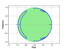
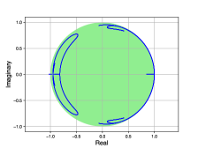
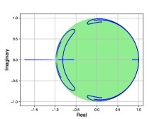
Figure 1: Eigenvalues and stability disks for different Poisson ratio. Top-left: 0; Top-right: 0.25; Bottom-left:0.3; Bottom-right: 0.4. The stability disk is plotted in green, and the eigenvalues in blue (refer to the web version of the article for the colors).

We observe that for a 45° directed wave vector, for a Poisson ratio different than $0.25$, there are some eigenvalues outside the stability disk, and particularly when the $\nu$ gets closer to the incompressible limit $0.5$. To investigate the other direction causing instability, we plotted on the $(k_{x},k_{y})$ plane, the points where some eigenvalues were outside the stability disk (i.e. with a modulus more than one). The results are shown in Figure 2.

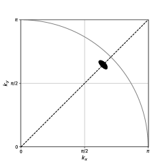
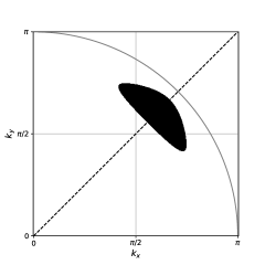
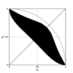
Figure 2: Unstable wave vectors for different Poisson ratio. Top-left: $\nu=0$; Top- right: $\nu=0.3$; Bottom-left: $\nu=0.35$; Bottom-right: $\nu=0.4$. The case $\nu=0.25$ is not shown since all wave vectors are stable. Only one quadrant is displayed due to the elementary symmetries of the set.

We see that for low Poisson ratio, the instability occurs only near the 45° direction and for high wave vectors only (near the $\pi$-radius circle). This results in 45°-direction instability pattern (see figure 3), after a long time (since only high wave-numbers are amplified, and since a Gaussian shape has very few high wave-numbers).

For high Poisson ratio, the domain of instability increases until all directions are unstable at high enough wave-numbers. This happens at $\nu=0.4$. Since we observe that instability occurs at lower wave-numbers for $\nu>0.25$ than for $\nu<0.25$, the high Poisson ratio simulations diverge more quickly. But is is useful noticing that only very high wave vectors are unstable, typically $|\mathbf{k}\Delta x|>\pi/3$ even at $\nu=0.4$. Therefore stable simulations can be recovered by refining the grid, or by filtering high frequencies at the end of a time step.

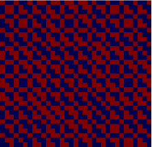
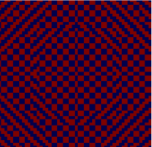
Figure 3: Example of instability patterns. Left: 45°; Right: all- directions. The color-map is saturated to blue-red colors due to great positive-negative values displayed: a sign of instability. In the 45° instability pattern, the diagonal stripes are spaces by $2.1$ spatial units. 45° patterns can be observed in low $\nu$ simulation after a long time, all-directions patterns can be observed in high $\nu$ simulation (here $\nu=0.4$).

For a Poisson ratio $\nu>0.25$ the velocity of P waves is greater than the lattice speed:

$$v_{P}(\nu>0.25)>\sqrt{3}v_{S}=1=\frac{\Delta x}{\Delta t}$$ (33)

It is a classic source of instability to have an information supposed to propagate faster than the lattice speed. This is another way of understanding the instability of Poisson ratio greater than $0.25$.

In fact, due to the second-order centered finite difference in the calculation of $\partial_{\alpha}\rho$ in (10), the information can in reality propagate at speed 2 instead of 1. So, the absolute limitation of $\nu$ beyond which $v_{P}$ would faster than 2 is $\nu_{lim}=5/11\approx 0.45$.

information is useful to understand that even with a stabilizing correction, the incompressible case $\nu=0.5$ is unreachable for regular sets with a definition of the ”sound speed” with S waves velocity $b=v_{S}$.

Nevertheless, the present method can be used for practical simulations. It is unconditionnaly stable for Poisson solids, i.e. $\nu=0.25$, and can be used for finite-time simulations for $\nu\neq 0.25$ at classical LBM CFL number. Since the instability arises only at high wave numbers.

5 Validation: Bulk wave propagation

As a first validation, one addresses the propagation of both P and S waves in the bulk of a 2D linear isotropic elastic medium. To this end, a $x$-force Gaussian source is placed in the middle of a domain periodic in $x$ and $y$ directions. The source is spatially Gaussian (instead of point source for example) to avoid high spatial frequencies (high wave numbers) which behave less precisely and can lead to instability. The typical radius of the source is 4 $\Delta x$. This source is modulated through time with a classic Ricker wavelet with a period of 20 $\Delta t$.

The D2Q9 simulation is compared with reference results obtained using a Fourier spectral method (with Crank-Nicolson time integration to allow for CFL=1, i.e. $\Delta x=\Delta t$ to correspond with the LBM iterations) for several reasons:

• 2D analytical solutions of the wave equation are not trivial (they make use of Bessel’s functions),

• The source is not point source (which would involve convolutions for an analytical solution),

• The simulation is periodic in both $x$ and $y$ directions.

The detail of this spectral method is explained in Appendix B.

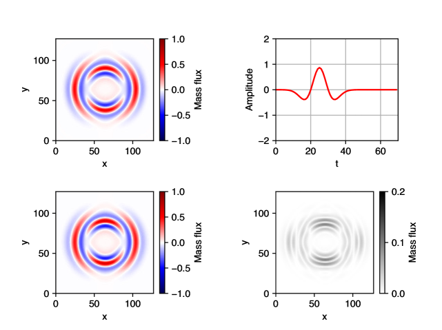
Figure 4: Comparison of $j_{x}$ for LBM D2Q9 with the Fourier spectral method, for Poisson ratio $\nu=0.1$. Top-left: LBM D2Q9; Bottom-left: Fourier spectral; Top-right: Ricker wavelet modulation of the source; Bottom-right: absolute difference of $j_{x}$ between the two models.

The simulations are performed on 64x64, 128x128, 256x256 and 512x512 grids using $\tau=0.55\Delta t$ along with $\nu=0.0,\ 0.1,\ 0.2,\ 0.25$ and $0.3$. Instantaneous results obtained at time $70\Delta t$ on the 128x128 grid for $\nu=0.1$ are displayed in Fig. 4. One can see that both LBM and spectral method capture the behaviour of P waves and S waves very accurately. The P waves are the ones on the left-right sides (the fastest travelling waves) and the S waves are the one on the top-bottom sides.

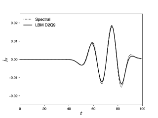
Figure 5: Comparison of the seismogram of the longitudinal mass flux $j_{x}$ for LBM D2Q9 with the spectral method, for a Poisson ratio $\nu=0$.

In order to quantify the difference between the LBM and the spectral method, a seismogram of a particular station (here $x=2N_{x}/3$,$y=2N_{y}/3$ ) is plotted in Fig. 5. It is observed that a very satisfactory agreement is recovered, even on a coarse grid for the LBM computation.

The accuracy of the LBM method is further investigated by measuring its effective order of convergence. The relative $L_{2}$ norm of the error committed on the longitudinal mass flux $j_{x}$ is defined as

$$p=\sqrt{\frac{\sum_{i,j=1,1}^{N_{x},N_{y}}\left(j_{x}^{\rm{LBM}}(i,j)-j_{x}^{\rm{spectral}}(i,j)\right)^{2}}{\sum_{i,j=1,1}^{N_{x},N_{y}}\left(j_{x}^{\rm{spectral}}(i,j)\right)^{2}}}$$ (34)

Values computed are given in Table 1 and plotted in Fig. 6. It is observed that the error exhibits a weak sensitivity to the Poisson ratio, which is a good property, and that a first order of convergence is obtained on the mass flux.

Table 1: $L_{2}$ norm of the error computed on the longitudinal mass flux $j_{x}$ for several combinations of the grid resolution $Nx\times N_{y}$ and the Poisson ratio $\nu$.

	$\nu=0$	$\nu=0.1$	$\nu=0.2$	$\nu=0.25$	$\nu=0.3$
$N_{x}=N_{y}=$ 64	0.2508	0.2351	0.2227	0.2185	0.2141
$N_{x}=N_{y}=$ 128	0.1112	0.1111	0.1137	0.1155	0.1164
$N_{x}=N_{y}=$ 256	0.0633	0.0644	0.0667	0.0678	0.0681
$N_{x}=N_{y}=$ 512	0.0349	0.0355	0.0366	0.0371	0.0371

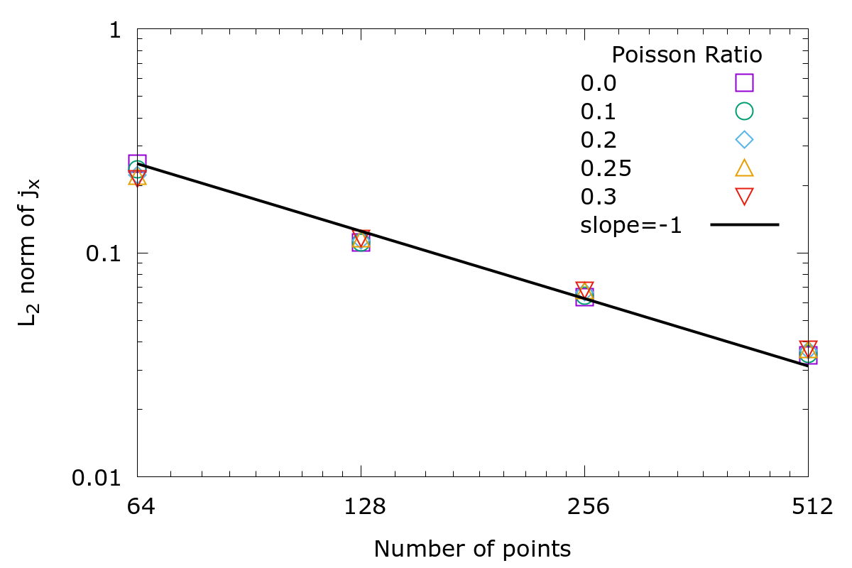
Figure 6: Grid convergence of the $L_{2}$ norm of the error on the longitudinal mass flux $j_{x}$.

To check the velocity of the bulk waves, some measurement of the travel time of P waves (time to reach the left-right borders from the center) and S waves (time to reach the top-bottom borders from the center) have been performed for several values of the Poisson ratio(see figure 7). The maximum relative error is 1.1% on the 128x128 grid, corresponding to a very accurate capture of the wave physics.

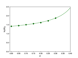
Figure 7: Comparison of the theoretical (dashed line) and LBM D2Q9 results (diamond markers) relation between $\nu$ and $v_{P}/v_{S}$

The present results show that the D2Q9 Lattice Boltzmann method yields very accurate prediction of bulk P and S waves, with an accuracy similar to those reported with other methods, e.g. [27, 25, 13, 35].

6 Boundary conditions

The developments given in [14] and in the above section were focused on the bulk wave propagation in infinite media, and only periodic boundary conditions were used. We now extend the method by deriving boundary conditions for more realistic cases: rigid interfaces with null displacement, free surface and non-reflecting outlet boundary condition.

6.1 Rigid wall boundary conditions

The simplest BC is probably the ”Bounce-Back” boundary condition (BB). For fluids it represents the no-slip condition, typically used to implement a steady solid wall in a viscous fluid, leading to (for instance for a bottom wall): $v_{x,wall}=0$ with $v$ the velocity. For solids, a rigid interface interface would mean $j_{x,wall}=0$, i.e. the displacement and the mass flux are null on the boundary. This would exist with the interface of our solid of interest with a rigid wall (for instance another solid with a much greater density or stiffness). The usual BB condition imposes the wall location to lie between two nodes :

$$y_{wall}=y_{b}+\frac{\Delta y}{2}\vec{n}$$ (35)

with $y_{b}$ the last layer near the interface and $\vec{n}$ the normal interface unit vector pointing outwards the solids. Therefore, the present Bounce Back condition is implemented as

$$f_{\bar{i}}(x_{b},t+\Delta t)=f_{i}(x_{b},t)$$ (36)

with $c_{\bar{i}}$ being the opposite of $c_{i}$: $c_{\bar{i}}=-c_{i}$

6.2 Free surface boundary condition

We consider now an interface with a medium with a much lower density and stiffness than the solid, e.g. gas or void. In the following, the case of the interface between the solid and air is used for the sake of clarity.

The solid/air interface location is $\Delta x/2$ far the last LBM node $x_{b}$ located in the solid medium:

$$x_{air}=x_{b}+\frac{\Delta x}{2}\vec{n}$$ (37)

with $\vec{n}$ the normal interface unit vector pointing outwards the solids. The bouncing condition is now :

$$f_{\bar{i}}(x_{b},t+\Delta x)=-f_{i}(x_{b},t)+2w_{i}\left(\rho_{air}+\frac{1}{2b^{4}}P^{n}_{\alpha\beta,air}\left(c_{i\alpha}c_{i\beta}-b^{2}\delta_{\alpha\beta}\right)\right)$$ (38)

where $\rho_{air}$ is the density estimated at the border with a linear interpolation

$$\rho_{air}=\frac{3}{2}\rho_{b}-\frac{1}{2}\rho_{in}$$ (39)

where $\rho_{in}$ is the density one node further inside the solid

$$x_{in}=x_{b}-\Delta x\vec{n}$$ (40)

The $P_{\alpha\beta,air}^{n}$ tensor at the interface is :

$$P_{\alpha\beta,air}^{n}=P_{\alpha\beta,air}-b^{2}\rho_{air}\delta_{\alpha\beta}$$ (41)

To explain how to find $P_{\alpha\beta,air}$, we consider the case of a vertical interface:

$$P_{\alpha\beta,air}=\begin{pmatrix}P_{xx,air}&0\\ 0&0\end{pmatrix}$$ (42)

because $P_{\alpha\beta,air}n_{\beta}=F_{\alpha}=0$, $F_{\alpha}$ is the force applied by air on the solid at the interface, which is assumed to be negligible in usual pressure and temperature conditions. $P_{xx,air}$ is obtained with linear interpolation similar to $\rho_{air}$.

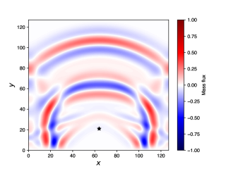
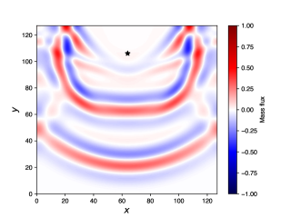
Figure 8: Test of the BCs: reflection of a vertical P wave on different interfaces. Left: bottom rigid wall (BB); Right: top free surface (ABB). The star marker indicates the position of the source

6.3 Validation of Rigid Wall and Free Surface boundary conditions

We now validate the two boundary conditions discussed above by considering wave reflection on these two kinds of boundaries.

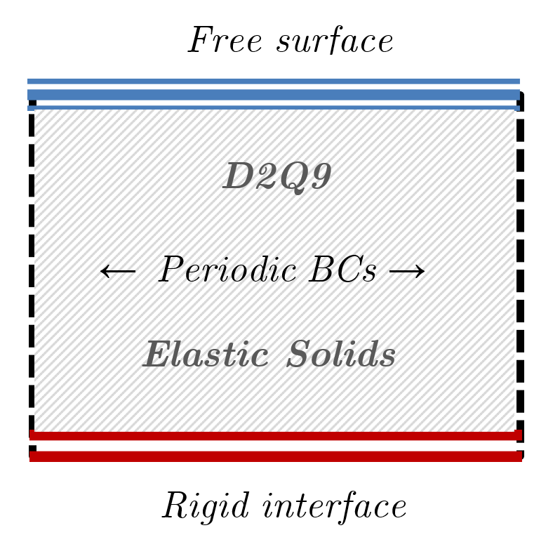
Figure 9: Configuration of the first BC test

To this end, a domain with periodic lateral conditions is defined, the BCs of interest being implemented on the top (free surface case) or bottom boundary (rigid wall case), as illustrated in Fig. 9. A directional source pointing vertically is added near the interface of interest. We observe that the waves are bouncing off these interfaces. The larger circle arc is the first P-wave with a direct path and the second concentric circle is the P-wave reflected.

Two criteria indicate that the boundary conditions are accurately implemented.

The first one deals with the sign of the velocity. For a free surface, there is no change in the sign of the speed (i.e. phase change) after the reflection, since the condition is a Neumann condition for velocity. For the rigid interface, there is a change in the sign of the speed (i.e. phase inversion) because it is a Dirichlet condition on velocity. This can be understood considering the following simplified mass flux equation:

$$\partial_{t}j_{\alpha}+\partial_{\beta}P_{\alpha\beta}=0$$ (43)

Considering an horizontal boundary at $y=0$, it leads to $\partial_{t}j=-\partial_{y}P$, yielding $P(c_{s}t\mp y)=\pm c_{s}j(c_{s}t\mp y)$, so that $P=0$ at the border is equivalent to $P(0,t)=P_{i}(c_{s}t-0)+P_{r}(c_{s}t+0)=0$, where the i and r subscripts are related to incident and reflected waves, respectively. For rigid walls with $j=0$, the Dirichlet condition gives the result in a straightforward way.

The second criterion is the speed magnitude at the border. For a free surface the incident and reflected wave interfere constructively while for the rigid interface, the interference is destructive. This is visible with a darker (respectively lighter) area near the border.

6.4 Absorbing layers for non-reflecting boundary conditions

To simulate a semi-infinite medium, we need to introduce non-reflecting boundary conditions in order to define outlet boundary conditions. Different approaches have been tested for fluids, based either on the use of improved BCs on the outlet plane or the implementation of sponge layers in which fluctuations are damped, or a combination of these two approaches. Numerical experiments performed in fluid LBM framework have shown that the use of a sponge layer is mandatory to get very accurate results for internal flows or on small computational domain.

Contrary to fluids where the viscosity can be changed with $\tau$ to introduce a progressive damping effect, the Chapman-Enskog-like analysis given above shows that $\tau$ doesn’t induce a viscous behaviour in the present case. Therefore, in the present solid LBM case, it is chosen to design absorbing layers. The principle is to smoothly increase a damping factor near the borders to completely remove the reflected waves. This is done by adding a linear penalty term in the mass flux equation:

$$\begin{split}&\partial_{t}\rho+\partial_{\alpha}j_{\alpha}=0\\ &\partial_{t}j_{\alpha}+\partial_{\beta}P_{\alpha\beta}=\frac{\mu-\lambda}{\rho_{0}}\partial_{\alpha}\rho-Aj_{\alpha}\\ &\partial_{t}P_{\alpha\beta}+\partial_{\gamma}Q_{\alpha\beta\gamma}^{eq}=0\end{split}$$ (44)

where $A$ is the damping factor and the term $-Aj_{\alpha}$ is treated as a forcing (exactly like an external forcing or the elastic artificial forcing).

The associated modified Navier equation is :

$$\partial_{t}^{2}j_{\alpha}+A\partial_{t}j_{\alpha}=\frac{\lambda+\mu}{\rho_{0}}\partial_{\alpha}\partial_{\beta}j_{\beta}+\frac{\mu}{\rho_{0}}\partial_{\beta}^{2}j_{\alpha}+\frac{1}{\rho_{0}}\partial_{t}F_{\alpha}$$ (45)

A plane-wave analysis shows that all modes are damped in the absorbing layer.

7 Validation: Rayleigh surface waves

The last validation case is related to the simulation of surface waves, that are very important in seismology. The motion being restricted in the plane in the present paper (2D simulations), the only surface waves possible are the Rayleigh waves (R waves). They stem from the combination of both P and S waves and their reflections at the surface. Their relative speed with P and S waves are also varying with the Poisson ratio but they are slightly slower than S waves. In the particular case of Poisson solids ($\nu=0.25$), $v_{R}=v_{S}\sqrt{0.8453}\approx 0.92v_{S}$ [36]. Rayleigh waves have an amplitude that decays exponentially with depth. The motion of the particle is ellipsoidal, like the the motion of particle of fluids in the swell. Rayleigh waves have been reported to be accurately captured using ELM (see [28, 26] and references given herein) but, to the knowledge of the authors, they have not been computed via LBM up to now.

To isolate and observe surface waves, the following numerical experiment has be conducted on a 100x300 computational grid. A free surface condition is implemented on the top boundary and the three remaining borders are treated with absorbing layers with a thickness of 30 nodes each.

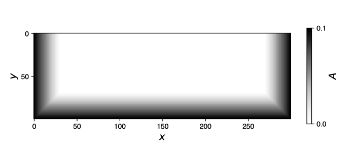
Figure 10: Absorbing layers

As a first step, absorbing layers are used to damp bulk S and P waves in order to isolate Rayleigh surface waves. In the second step, absorbing layers are removed and periodic conditions are imposed on lateral boundaries in order to let the Rayleigh waves propagate freely. The source is located on the upper left corner so that all waves going to the left are quickly removed (absorbed by the left sponge layer). The fastest wave (P waves) going to the right are also removed by the right absorbing layer, then (after 400 time steps) the left-right absorbing layers are replaced by a simple left-right periodic condition.

A 2D circular bulk wave with constant energy has a typical amplitude decaying as $1/\sqrt{r}$ while a surface wave in the present case will be a 1D wave, whose amplitude will be constant in the energy-preserving case. Thanks to that difference, surface waves should last longer than the S waves that are travelling to the right just slightly faster).

The results are displayed in Fig. 11. The simulation qualitatively captures the behaviour of Rayleigh waves. At time steps 600 and 1200 there remains some S waves also going to the right because they are only slightly faster than Rayleigh waves (at $\nu=0.25$, $v_{R}\approx 92\%v_{S}$). The speed of R waves have been measured with a 0.14% relative error, by measuring the number of time steps needed to achieve for two complete turns around the periodic surface:

$$\begin{split}v_{R}^{\rm{measured}}=0.5315,\quad v_{R}^{\rm{theo}}=\sqrt{\frac{0.8453}{3}}=0.5308\end{split}$$ (46)

However, the amplitude of these Rayleigh waves is slowly decreasing. This is consequence of the error term found in Eq. (28) and underlined in the Von Neumann analysis.

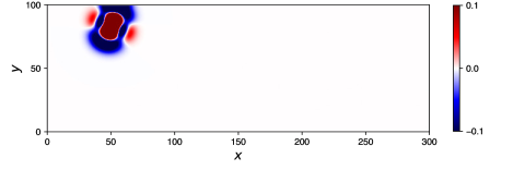
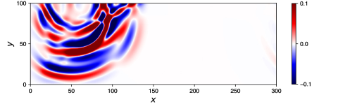
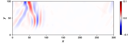
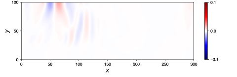
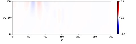
Figure 11: Vertical mass flux profile at different time, for $\nu=0.25$. The star marker indicates the position of the source. From top to bottom: iteration 30, 100, 600, 1200, 1800

The exponential decreasing amplitude with depth has been plotted for a vertical slice at the time step 1800, at position $x=83$. In fact this time was chosen, despite the weak amplitude, because the remaining S waves and other artefacts are clearly separated. The results are displayed in the Figure 12.

The exponential model is simply

$$j_{y}=A\exp(-y/d)$$ (47)

With the exponential regression (fitting with the amplitude $A$ and the typical depth $d$), we see that the damping is approximately of the exponential form, yet, the amplitude near the surface has a bump. In fact, a rigorous study of the analytical solution for the Rayleigh equation gives a more complex solution [37]:

$$j_{y}=-\alpha_{S}\left[\exp(-k\alpha_{S}y)-\frac{2}{1+\alpha_{P}^{2}}\exp(-k\alpha_{P}y)\right]$$ (48)

with $\alpha_{S}\equiv\sqrt{1-v_{R}^{2}/v_{S}^{2}}$ and $\alpha_{P}\equiv\sqrt{1-v_{R}^{2}/v_{P}^{2}}$.

This analytical model was integrated and fitted with the amplitude and the wavelength $\lambda_{R}$ of the wave (giving $k=2\pi/\lambda_{R}$). It can be observed that the simulation results show a better match with these analytical results and the regression even recovers the correct wavelength $\lambda_{R}$ (within 1.3% error) that can be also measured between two maxima of the mass flux.

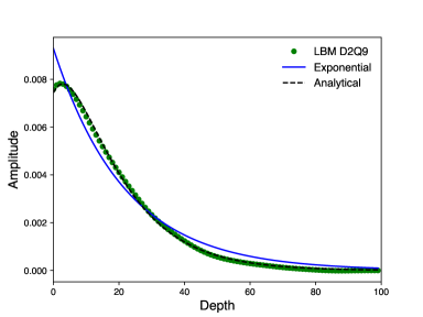
Figure 12: Profile of the amplitude of the mass flux in a vertical section $x=83$ at the iteration 1800. The regression were done with the least square method. For the exponential model the amplitude was $A=0.0093$, the typical depth $d=21.9$ and the residue is of order $10^{-5}$. For the analytical model, the amplitude is 0.012, the wavelength is$\lambda_{R}=37.1$ and the residue is of order $10^{-7}$

These results clearly show that the present solid LBM is able to accurately capture surface waves, and that the proposed boundary conditions for rigid surfaces, free surfaces and sponge layers are efficient.

8 Conclusions

The Lattice Boltzmann method proposed in [14] has been extended in several ways, by i) using a regular lattice in place of the more complex Crystallographic Lattice used in the original version, ii) defining boundary conditions for free surface and rigid surfaces and iii) introducing efficient sponge layer technique to prevent spurious wave reflection. These new elements have been supplemented by two theoretical analyses, i.e. the Chapman-Enskog expansion to recover the associated macroscopic equations and the von-Neumann-type linearized stability analysis.

It is shown that the method the first-order accurate considering the $L_{2}$ norm of the error on the mass flux, and that the method is unconditionnally stable for Poisson solids and stable for low-wave-number solution for other values of the Poisson ratio $\nu$.

Numerical experiments have demonstrated the accuracy of the present method for both bulk and surface waves and, to the knowledge of the authors, it is the first time that surface waves are successfully computed using a Lattice Boltzmann method for elastic solids.

Appendix A. Chapman-Enskog Analysis

The moment $R^{eq}_{\alpha\beta\gamma\kappa}$ for regular lattices is

$$\begin{split}R_{\alpha\beta\gamma\kappa}^{eq}&=\rho b^{4}\Delta^{(4)}_{\alpha\beta\gamma\kappa}+\frac{1}{2b^{4}}P^{n}_{\theta\psi}\left(\sum_{i}w_{i}c_{i\alpha}c_{i\beta}c_{i\gamma}c_{i\kappa}c_{i\theta}c_{i\psi}-b^{2}\delta_{\theta\psi}\sum_{i}w_{i}c_{i\alpha}c_{i\beta}c_{i\gamma}c_{i\kappa}\right)\\ &=\rho b^{4}\Delta^{(4)}_{\alpha\beta\gamma\kappa}+\frac{b^{2}}{2}P^{n}_{\theta\psi}\left(\Delta^{(6)}_{\alpha\beta\gamma\kappa\theta\psi}-6\delta_{\alpha\beta\gamma\kappa\theta\psi}-\delta_{\theta\psi}\Delta^{(4)}_{\alpha\beta\gamma\kappa}\right)\\ &=\rho b^{4}\Delta^{(4)}_{\alpha\beta\gamma\kappa}+\frac{b^{2}}{2}\left(P^{n}_{\alpha\psi}\Delta^{(4)}_{\beta\gamma\kappa\psi}+P^{n}_{\beta\psi}\Delta^{(4)}_{\alpha\gamma\kappa\psi}+P^{n}_{\gamma\psi}\Delta^{(4)}_{\alpha\beta\kappa\psi}+P^{n}_{\kappa\psi}\Delta^{(4)}_{\alpha\beta\gamma\psi}-6P^{n}_{\psi\psi}\delta_{\alpha\beta\gamma\kappa\psi}\right)\\ &=\rho b^{4}\Delta^{(4)}_{\alpha\beta\gamma\kappa}+b^{2}\left(P^{n}_{\alpha\beta}\delta_{\gamma\kappa}+P^{n}_{\alpha\gamma}\delta_{\beta\kappa}+P^{n}_{\alpha\kappa}\delta_{\beta\gamma}+P^{n}_{\beta\gamma}\delta_{\alpha\kappa}+P^{n}_{\beta\kappa}\delta_{\alpha\gamma}+P^{n}_{\lambda\kappa}\delta_{\alpha\beta}-3P^{n}_{\psi\psi}\delta_{\alpha\beta\gamma\kappa\psi}\right)\end{split}$$ (49)

Taking a spatial derivative $\partial^{(1)}_{\kappa}$ of the above moment gives

$$\begin{split}\partial^{(1)}_{\kappa}R_{\alpha\beta\gamma\kappa}^{eq}=&\rho b^{4}\left(\delta_{\beta\gamma}\partial_{\alpha}^{(1)}\rho+\delta_{\alpha\gamma}\partial_{\beta}^{(1)}\rho+\delta_{\alpha\beta}\partial_{\gamma}^{(1)}\rho\right)+b^{2}\left(\partial_{\alpha}^{(1)}P^{n}_{\beta\gamma}+\partial_{\beta}^{(1)}P^{n}_{\alpha\gamma}+\partial_{\gamma}^{(1)}P^{n}_{\alpha\beta}\right)\\ &+b^{2}\partial_{\kappa}^{(1)}\left(P^{n}_{\alpha\kappa}\delta_{\beta\gamma}+P^{n}_{\beta\kappa}\delta_{\alpha\gamma}+P^{n}_{\gamma\kappa}\delta_{\alpha\beta}-3P^{n}_{\psi\psi}\delta_{\alpha\beta\gamma\kappa\psi}\right)\\ =&b^{2}\left(\partial_{\alpha}^{(1)}P_{\beta\gamma}+\partial_{\beta}^{(1)}P_{\alpha\gamma}+\partial_{\gamma}^{(1)}P_{\alpha\beta}+\partial_{\kappa}^{(1)}\left(P^{n}_{\alpha\kappa}\delta_{\beta\gamma}+P^{n}_{\beta\kappa}\delta_{\alpha\gamma}+P^{n}_{\gamma\kappa}\delta_{\alpha\beta}-3P^{n}_{\kappa\kappa}\delta_{\alpha\beta\gamma\kappa}\right)\right).\end{split}$$ (50)

The time derivative of $Q_{\alpha\beta\gamma}^{eq}$ can be computed using Eq. (12) and replacing the $\partial_{t}^{(1)}j_{\alpha}$ terms with $-\partial_{\kappa}^{(1)}P_{\alpha\kappa}+S_{\alpha}^{(1)}$ via Eq. (25) to be

$$\begin{split}\partial_{t}^{(1)}Q_{\alpha\beta\gamma}^{eq}=&b^{2}\partial_{t}^{(1)}\left(j_{\alpha}\delta_{\beta\gamma}+j_{\beta}\delta_{\alpha\gamma}+j_{\gamma}\delta_{\alpha\beta}\right)\\ =&-b^{2}\partial_{\kappa}^{(1)}\left(P_{\alpha\kappa}\delta_{\beta\gamma}+P_{\beta\kappa}\delta_{\alpha\gamma}+P_{\alpha\kappa}\delta_{\alpha\beta}\right)\\ &+b^{2}\left(S^{(1)}_{\alpha}\delta_{\beta\gamma}+S^{(1)}_{\beta}\delta_{\alpha\gamma}+S^{(1)}_{\gamma}\delta_{\alpha\beta}\right)\end{split}$$ (51)

Using the above relations $Q_{\alpha\beta\gamma}^{(1)}$ can be calculated from the final equation of Eq. (25) to be

$$\begin{split}Q_{\alpha\beta\gamma}^{(1)}=&-\tau\left[\partial_{t}^{(1)}Q_{\alpha\beta\gamma}^{eq}+\partial^{(1)}_{\kappa}R_{\alpha\beta\gamma\kappa}^{eq}-b^{2}\left(1-\frac{\Delta t}{2\tau}\right)\left(S^{(1)}_{\alpha}\delta_{\beta\gamma}+S^{(1)}_{\beta}\delta_{\alpha\gamma}+S^{(1)}_{\gamma}\delta_{\alpha\beta}\right)\right]\\ =&-\tau b^{2}\left[\partial_{\alpha}^{(1)}P^{n}_{\beta\gamma}+\partial_{\beta}^{(1)}P^{n}_{\alpha\gamma}+\partial_{\gamma}^{(1)}P^{n}_{\alpha\beta}-3\partial_{\kappa}^{(1)}P_{\kappa\kappa}^{n}\delta_{\alpha\beta\gamma\kappa}\right]\\ &-b^{2}\left[\frac{\Delta t}{2}\left(S^{(1)}_{\alpha}\delta_{\beta\gamma}+S^{(1)}_{\beta}\delta_{\alpha\gamma}+S^{(1)}_{\gamma}\delta_{\alpha\beta}\right)\right]\end{split}$$ (52)

Appendix B. Custom Fourier spectral method

A Fourier spectral method with Crank-Nicholson time integration is used to compare bulk waves. We define $(\hat{j_{x}},\hat{j_{y}})^{T}$ as the spatial Fourier transform of the mass flux vector $(j_{x},j_{y})^{T}$. Let the $\hat{J}$ vector be

$$\hat{J}=\begin{pmatrix}\hat{j_{x}}\\ \hat{j_{y}}\\ \partial_{t}\hat{j_{x}}\\ \partial_{t}\hat{j_{y}}\end{pmatrix}.$$ (53)

To simplify the notation, we denote $a^{2}=(\lambda+2\mu)/\rho_{0}$, $b^{2}=\mu/\rho_{0}$ and $d^{2}=(\lambda+\mu)/\rho_{0}$, such that the Navier equation for $j_{x}$ and $j_{y}$ in the Fourier domain can be written as

$$\begin{split}&\partial_{tt}\hat{j_{x}}=-a^{2}k_{x}^{2}\hat{j_{x}}-d^{2}k_{x}k_{y}\hat{j_{y}}-b^{2}k_{y}^{2}\hat{j_{x}}+\frac{1}{\rho_{0}}\partial_{t}\hat{F_{x}}\\ &\partial_{tt}\hat{j_{y}}=-b^{2}k_{x}^{2}\hat{j_{y}}-d^{2}k_{x}k_{y}\hat{j_{x}}-a^{2}k_{y}^{2}\hat{j_{y}}+\frac{1}{\rho_{0}}\partial_{t}\hat{F_{y}}\end{split}$$ (54)

Hence,

$$\partial_{t}\hat{J}=\begin{pmatrix}\partial_{t}\hat{j_{x}}\\ \partial_{t}\hat{j_{y}}\\ -a^{2}k_{x}^{2}\hat{j_{x}}-d^{2}k_{x}k_{y}\hat{j_{y}}-b^{2}k_{y}^{2}\hat{j_{x}}+\frac{1}{\rho_{0}}\partial_{t}\hat{F_{x}}\\ -b^{2}k_{x}^{2}\hat{j_{y}}-d^{2}k_{x}k_{y}\hat{j_{x}}-a^{2}k_{y}^{2}\hat{j_{y}}+\frac{1}{\rho_{0}}\partial_{t}\hat{F_{y}}\end{pmatrix}$$ (55)

This equation is of the form $\partial_{t}\hat{J}=f\left(\hat{J},\hat{F}\right)$. The Crank-Nicholson scheme is A-Stable, which allows us to take $\Delta t=\Delta x$, furthermore, it is a symplectic integrator, which is beneficial for equations of the form $\ddot{X}+\omega^{2}X=0$ like (55).

The Crank-Nicholson scheme is

$$\hat{J}_{n+1}=\hat{J}_{n}+\frac{\Delta t}{2}\left[f\left(\hat{J}_{n}\right)+f\left(\hat{J}_{n+1}\right)\right]$$ (56)

On simplification, the above equations can be evaluated in matrix form to be

$$M\hat{J}_{n+1}=N\begin{pmatrix}\hat{J}_{n}\\ \hat{G}_{x}\\ \hat{G}_{y}\end{pmatrix},$$ (57)

hence,

$$\hat{J}_{n+1}=M^{-1}N\begin{pmatrix}\hat{J}_{n}\\ \hat{G}_{x}\\ \hat{G}_{y}\end{pmatrix}$$ (58)

with

$$\begin{split}&\hat{G}_{x}=\frac{1}{\rho_{0}}\left(\partial_{t}\hat{F}_{x,n}+\partial_{t}\hat{F}_{x,n+1}\right)\\ &\hat{G}_{y}=\frac{1}{\rho_{0}}\left(\partial_{t}\hat{F}_{y,n}+\partial_{t}\hat{F}_{y,n+1}\right),\end{split}$$ (59)

$$M=\begin{pmatrix}1&0&-\frac{\Delta t}{2}&0\\ 0&1&0&-\frac{\Delta t}{2}\\ \frac{A\Delta t}{2}&\frac{B\Delta t}{2}&1&0\\ \frac{B\Delta t}{2}&\frac{C\Delta t}{2}&0&1\end{pmatrix}$$ (60)

$$N=\begin{pmatrix}1&0&\frac{\Delta t}{2}&0&0&0\\ 0&1&0&\frac{\Delta t}{2}&0&0\\ \frac{-A\Delta t}{2}&\frac{-B\Delta t}{2}&1&0&\frac{\Delta t}{2}&0\\ \frac{-B\Delta t}{2}&\frac{-C\Delta t}{2}&0&1&0&\frac{\Delta t}{2}\end{pmatrix}$$ (61)

and,

$$\begin{split}&A=a^{2}k_{x}^{2}+b^{2}k_{y}^{2}\\ &B=d^{2}k_{x}k_{y}\\ &C=a^{2}k_{y}^{2}+b^{2}k_{x}^{2}\end{split}$$ (62)

Then the equation (58) is just a simple matrix relation that can be iterated along with the LBM. When needed, the mass flux can be obtained by an inverse Fourier transform.

References

- [1] T. Kruüger, H. Kusumaatmaja, A. Kuzmin, O. Shardt, G. Silva, E. Viggen, The Lattice Boltzmann Method. Principles and Practice, Springer, 2017.
- [2] Z. Guo, C. Shu, The Lattice Boltzmann Method and its applications in engineering, World Scientific, 2013.
- [3] J. Jacob, O. Malaspinas, P. Sagaut, A new hybrid recursive regularised bhatnagar–gross–krook collision model for lattice boltzmann method-based large eddy simulation, Journal of Turbulence 19 (11-12) (2018) 1051–1076.
- [4] Y. Feng, P. Boivin, J. Jacob, P. Sagaut, Hybrid recursive regularized thermal lattice boltzmann model for high subsonic compressible flows, Journal of Computational Physics 394 (2019) 82–99.
- [5] S. Guo, Y. Feng, J. Jacob, P. Sagaut, An efficient lattice Boltzmann method for industrial aerodynamics flows, I: basic model on D3Q19 lattice, Journal of Computational Physics 418 (2020) 109570.
- [6] P. Dellar, Lattice boltzmann formulation for linear viscoelastic fluids using an abstract second stress, SIAM Journal of Scientific Computing 36 (2014).
- [7] Y. Guangwu, A lattice boltzmann equation for waves, Journal of Computational Physics 161 (2000) 61–69.
- [8] W. Jiaung, J. Ho, C. Kuo, Lattice boltzmann method for the heat conduction problem with phase change, Numerical Heat Transfer, Part B 39 (2001).
- [9] L. Zhiong, S. Feng, P. Dong, S. Gao, Lattice boltzmann schemes for the nonlinear schrödinger equation, Physical Review E 74 (2006).
- [10] S. Hasanoge, S. Succi, S. Orszag, Lattice boltzmann method for electromagnetic wave propagation, EuroPhysics Letters 96 (2011).
- [11] Y. Liu, G. Yan, A lattice Boltzmann Model for maxwell’s equations, Applied Mathematical Modelling 38 (2014).
- [12] X. Yin, G. Yan, T. Li, Direct simulations of the linear elastic displacements field based on a lattice Boltzmann model: Direct simulations of the linear elastic displacements field based on a lattice Boltzmann model, Int. J. Numer. Meth. Engng 107 (3) (2016) 234–251. doi:10.1002/nme.5167.
- [13] G. S. O’Brien, T. Nissen-Meyer, C. J. Bean, A Lattice Boltzmann Method for Elastic Wave Propagation in a Poisson Solid, Bulletin of the Seismological Society of America 102 (3) (2012) 1224–1234. doi:10.1785/0120110191.
- [14] J. S. N. J.Murthy, P. K. Kolluru, V. Kumaran, S. Ansumali, Lattice Boltzmann Method for Wave Propagation in Elastic Solids, CiCP 23 (4) (2018). doi:10.4208/cicp.OA-2016-0259.
- [15] S. Xiao, A lattice Boltzmann method for shock wave propagation in solids, Communications in Numerical Methods in Engineering 23 (2007).
- [16] M. Namburi, S. Krithivasan, S. Ansumali, Crystallographic Lattice Boltzmann Method, Sci Rep 6 (1) (2016) 27172. doi:10.1038/srep27172.
- [17] P. K. Kolluru, M. Atif, M. Namburi, S. Ansumali, Lattice boltzmann model for weakly compressible flows, Physical Review E 101 (1) (2020) 013309.
- [18] I. Ispolatov, M. Grant, Lattice boltzmann method for viscoelastic fluids, Physical Review E 65 (2002).
- [19] P. Lallemand, D. d’Humieres, L. Luo, R. Rubinstein, Theory of the lattice boltzmann method: Three-dimensional model for the linear viscoelastic fluids, Physical Review E 67 (2003).
- [20] O. Malaspinas, N. Fétier, M. Deville, Lattice boltzmann method for the simulation of viscoelastic fluid flows, Journal of Non-Newtonian Fluid Mechanics 165 (2010).
- [21] T. Phillips, G. Roberts, Lattice boltzmann models for non-newtonian flows, Journal of Applied Mathematics 76 (2011).
- [22] G. N. Frantziskonis, Lattice Boltzmann method for multimode wave propagation in viscoelastic media and in elastic solids, Phys. Rev. E 83 (6) (2011) 066703. doi:10.1103/PhysRevE.83.066703.
- [23] A. Gupta, M. Sbragaglia, A. Scagliarini, Hybrid lattice boltzmann/finite difference simulations of viscoelastic multicomponent flows in confined gepmetries, Journal of Computational Physics 291 (2015).
- [24] G. O’Brien, C. Bean, A 3d discrete numerical elastic lattice method for seismic wave propagation in heterogeneous media with topography, Geophysical Research Letters 31 (2004).
- [25] G. O’Brien, C. Bean, An irregular lattice method for elastic wave propagation, Geophysical Journal International 187 (2011).
- [26] G. O’Brien, Elastic lattice modelling of seismic waves including a free surface, Computers and Geosciences 67 (2014).
- [27] G. O’Brien, Dispersion analysis and computational efficiency of elastic lattice methods for seismic wave propagation, Computers and Geosciences 35 (2009).
- [28] R. del Valle-Garcia, F. Sanchez-Sesma, Rayleigh waves modeling using an elastic lattice model, Geophysical Research Letters 30 (2003).
- [29] M. Xia, H. Zhou, Q. Li, H. Chen, Y. Wang, S. Wang, A general 3d lattice spring model for modeling elastic waves, Bulletin of the Seismological Society of America 107 (2017).
- [30] D. Polyzos, D. Fotiadis, Derivation of mindlin’s first and second strain gradient elastic theory via simple lattice and continuum models, International Journal of Solids and Structures 49 (2012).
- [31] S. Godunov, E. Romenskii, Elements of continuum mechanics and conservation laws, Springer, 2003.
- [32] H. Chen, X. Shan, Fundamental conditions for N-th-order accurate lattice Boltzmann models, Physica D: Nonlinear Phenomena 237 (14-17) (2008) 2003–2008. doi:10.1016/j.physd.2007.11.010.
- [33] T. Sengupta, A. Dipankar, P. Sagaut, Error dynamics: Beyond von Neumann analysis, Journal of Computational Physics 226 (2007).
- [34] G. Wissocq, P. Sagaut, J.-F. Boussuge, An extended spectral analysis of the lattice Boltzmann method: modal interactions and stability issues, Journal of Computational Physics 380 (2019) 311–333. doi:10.1016/j.jcp.2018.12.015.
- [35] M. Xia, S. Wang, H. Zhou, X. Shan, H. Chen, Q. Li, Q. Zhang, Modelling viscoacoustic wave propagation with the lattice Boltzmann method, Sci Rep 7 (1) (2017) 10169. doi:10.1038/s41598-017-10833-w.
- [36] K. Aki, P. G. Richards, Quantitative seismology, 2nd Edition, Univ. Science Books, Sausalito, Calif, 2009, oCLC: 845610339.
- [37] M. Destrade, G. Saccomandi, Linear Elastodynamics and Waves 36.