Searching for a Search Method: Benchmarking Search Algorithms for Generating NLP Adversarial Examples

Abstract

We study the behavior of several black-box search algorithms used for generating adversarial examples for natural language processing (NLP) tasks. We perform a fine-grained analysis of three elements relevant to search: search algorithm, search space, and search budget. When new search algorithms are proposed in past work, the attack search space is often modified alongside the search algorithm. Without ablation studies benchmarking the search algorithm change with the search space held constant, one cannot tell if an increase in attack success rate is a result of an improved search algorithm or a less restrictive search space. Additionally, many previous studies fail to properly consider the search algorithms’ run-time cost, which is essential for downstream tasks like adversarial training. Our experiments provide a reproducible benchmark of search algorithms across a variety of search spaces and query budgets to guide future research in adversarial NLP. Based on our experiments, we recommend greedy attacks with word importance ranking when under a time constraint or attacking long inputs, and either beam search or particle swarm optimization otherwise.

1 Introduction

Research has shown that current deep neural network models lack the ability to make correct predictions on adversarial examples Szegedy et al. (2013). The field of investigating the adversarial robustness of NLP models has seen growing interest, both in contributing new attack methods for generating adversarial examples Ebrahimi et al. (2017); Gao et al. (2018); Alzantot et al. (2018); Jin et al. (2019); Ren et al. (2019); Zang et al. (2020) and better training strategies to make models resistant to adversaries Jia et al. (2019); Goodfellow et al. (2014).

Recent studies formulate NLP adversarial attacks as a combinatorial search task and feature the specific search algorithm they use as the key contribution Zhang et al. (2019b). The search algorithm aims to perturb a text input with language transformations such as misspellings or synonym substitutions in order to fool a target NLP model when the perturbation adheres to some linguistic constraints (e.g., edit distance, grammar constraint, semantic similarity constraint) Morris et al. (2020a). Many search algorithms have been proposed for this process, including varieties of greedy search, beam search, and population-based search.

The literature includes a mixture of incomparable and unclear results when comparing search strategies since studies often fail to consider the other two necessary primitives in the search process: the search space (choice of transformation and constraints) and the search budget (in queries to the victim model). The lack of a consistent benchmark on search algorithms has hindered the use of adversarial examples to understand and to improve NLP models. In this work, we attempt to clear the air by answering the following question: Which search algorithm should NLP researchers pick for generating NLP adversarial examples?

We focus on black-box search algorithms due to their practicality and prevalence in the NLP attack literature. Our goal is to understand to what extent the choice of search algorithms matter in generating text adversarial examples and how different search algorithms compare when we hold the search space constant or when we standardize the search cost. We select three families of search algorithms proposed from literature and benchmark their performance on generating adversarial examples for sentiment classification and textual entailment tasks. Our main findings can be summarized as the following:

• Across three datasets and three search spaces, we found that beam search and particle swarm optimization are the best algorithms in terms of attack success rate.

• When under a time constraint or when the input text is long, greedy with word importance ranking is preferred and offers sufficient performance.

• Complex algorithms such as PWWS Ren et al. (2019) and genetic algorithm Alzantot et al. (2018) are often less performant than simple greedy methods both in terms of attack success rate and speed.

2 Background

2.1 Components of an NLP Attack

Morris et al. (2020b) formulated the process of generating natural language adversarial examples as a system of four components: a goal function, a set of constraints, a transformation, and a search algorithm.

Such a system searches for a perturbation from ${\mathbf{x}}$ to ${\mathbf{x}}^{\prime}$ that fools a predictive NLP model by both achieving some goal (like fooling the model into predicting the wrong classification label) and fulfilling certain constraints. The search algorithm attempts to find a sequence of transformations that results in a successful perturbation.

2.2 Elements of a Search Process

Search Algorithm:

Recent methods proposed for generating adversarial examples in NLP frame their approach as a combinatorial search problem. This is necessary because of the exponential nature of the search space. Consider the search space for an adversarial attack that replaces words with synonyms: If a given sequence of text consists of $W$ words, and each word has $T$ potential substitutions, the total number of perturbed inputs to consider is $(T+1)^{W}-1$. Thus, the graph of all potential adversarial examples for a given input is far too large for an exhaustive search.

While heuristic search algorithms cannot guarantee an optimal solution, they can be employed to efficiently search this space for a valid adversarial example. Studies on NLP attacks have explored various heuristic search algorithms, including beam search Ebrahimi et al. (2017), genetic algorithm Alzantot et al. (2018), and greedy method with word importance ranking Gao et al. (2018); Jin et al. (2019); Ren et al. (2019).

Search Space:

In addition to its search method, an NLP attack is defined by how it chooses its search space. The search space is mainly determined by two things: a transformation, which defines how the original text is perturbed (e.g. word substitution, word deletion) and the set of linguistic constraints (e.g minimum semantic similarity, correct grammar) enforced to ensure that the perturbed text is a valid adversarial example. A larger search space corresponds to a looser definition of a valid adversarial example. With a looser definition, the search space includes more candidate adversarial examples. The more candidates there are, the more likely the search is to find an example that fools the victim model – thereby achieving a higher attack success rate Morris et al. (2020b).

Search Cost/Budget:

Furthermore, most works do not consider the runtime of the search algorithms. This has created a large, previously unspoken disparity in runtimes of proposed works. Population-based algorithms like Alzantot et al. (2018) and Zang et al. (2020) are significantly more expensive than greedy algorithms like Jin et al. (2019) and Ren et al. (2019). Additionally, greedy algorithms with word importance ranking are linear with respect to input length, while beam search algorithms are quadratic. In tasks such as adversarial training, adversarial examples must be generated quickly, and a more efficient algorithm may preferable– even at the expense of a lower attack success rate.

2.3 Evaluating Novel Search Algorithms

Past studies on NLP attacks that propose new search algorithms often also propose a slightly altered search space, by proposing either new transformations or new constraints. When new search algorithms are benchmarked in a new search space, they cannot be easily compared with search algorithms from other attacks.

To show improvements over a search method from previous work, a new search method must be benchmarked in the search space of the original method. However, many works fail to set the search space to be consistent when comparing their method to baseline methods. For example, Jin et al. (2019) compares its TextFooler method against Alzantot et al. (2018)’s method without accounting for the fact that TextFooler uses the Universal Sentence Encoder Cer et al. (2018) to filter perturbed text while Alzantot et al. (2018) uses Google 1 billion words language model Chelba et al. (2013). A more severe case is Zhang et al. (2019a), which claims that its Metropolis-Hastings sampling method is superior to Alzantot et al. (2018) without setting any constraints – like Alzantot et al. (2018) does – that ensure that the perturbed text preserves the original semantics of the text.

We do note that Ren et al. (2019) and Zang et al. (2020) do provide comparisons where the search spaces are consistent. However, these works consider a small number of search algorithms as baseline methods, and fail to provide a comprehensive comparison of methods proposed in the literature.

3 Benchmarking Setup

3.1 Defining Search Spaces

As defined in Section 2.1, each NLP adversarial attack includes four components: a goal function, constraints, a transformation, and a search algorithm. We define the attack search space as the set of perturbed text ${\mathbf{x}}^{\prime}$ that are generated for an original input ${\mathbf{x}}$ via valid transformations and satisfy a set of linguistic constraints. The goal of a search algorithm is to find those ${\mathbf{x}}^{\prime}$ that achieves the attack goal function (i.e. fooling a victim model) as fast as it can.

Word-swap transformations:

Assuming ${\mathbf{x}}=(x_{1},\dots,x_{i},\dots,x_{n})$, a perturbed text ${\mathbf{x}}^{\prime}$ can be generated by swapping ${\mathbf{x}}_{i}$ with altered ${\mathbf{x}}^{\prime}_{i}$. The swap can occur at word, character, or sentence level, depending on the granularity of ${\mathbf{x}}_{i}$. Most works in literature choose to swap out words; therefore, we choose to focus on word-swap transformations for our experiments.

Constraints:

Morris et al. (2020b) proposed a set of linguistic constraints to enforce that ${\mathbf{x}}$ and perturbed ${\mathbf{x}}^{\prime}$ should be similar in both meaning and fluency to make ${\mathbf{x}}^{\prime}$ a valid potential adversarial example. This indicates that the search space should ensure ${\mathbf{x}}$ and ${\mathbf{x}}^{\prime}$ are close in semantic embedding space. Multiple automatic constraint ensuring strategies have been proposed in the literature. For example, when swapping word ${\mathbf{x}}_{i}$ with ${\mathbf{x}}^{\prime}_{i}$, we can require that the cosine similarity between word embedding vectors $e_{{\mathbf{x}}_{i}}$ and $e_{{\mathbf{x}}^{\prime}_{i}}$ meet certain minimum threshold. More details on the specific constraints we use are in Section A.1.

Now we use notation $T({\mathbf{x}})={\mathbf{x}}^{\prime}$ to denote transformations perturbing ${\mathbf{x}}$ to ${\mathbf{x}}^{\prime}$, and assume the $j-th$ constraints as Boolean functions $C_{j}({\mathbf{x}},{\mathbf{x}}^{\prime})$ indicating whether ${\mathbf{x}}^{\prime}$ satisfies the constraint $C_{j}$. Then, we can define the search space $S$ mathematically as:

$$S({\mathbf{x}})=\{T({\mathbf{x}})|C_{j}({\mathbf{x}},T({\mathbf{x}}))\;\forall j\in[m]\}$$ (1)

The goal of a search algorithm is to find ${\mathbf{x}}^{\prime}\in S(x)$ such that ${\mathbf{x}}^{\prime}$ succeeds in fooling the victim model. Table 1 describes three search spaces we use to benchmark the search algorithms. Details of transformations and constraints used in defining these search spaces are in Appendix Section A.1.

	Transformation	Constraints
1	Counter-fitted GLOVE Word Embedding	Word embedding similarity, BERTScore, POS consistency
2	HowNet	BERTScore, POS consistency
3	WordNet	USE similarity, POS consistency

Table 1: The three search spaces in our benchmarking.

Search Algorithm	Deterministic?	Hyperparameters	Num. Queries
Beam Search Ebrahimi et al. (2017)	✓	$b$ (beam width)	$\mathcal{O}(b*W^{2}*T)$
Greedy [Beam Search with b=1]	✓	–	$\mathcal{O}(W^{2}*T)$
Greedy w. Word Importance Ranking Gao et al. (2018); Jin et al. (2019); Ren et al. (2019)	✓	–	$\mathcal{O}(W*T)$
Genetic Algorithm Alzantot et al. (2018)	✗	$p$ (population size), $g$ (number of iterations)	$\mathcal{O}(g*p*T)$
Particle Swarm Optimization Zang et al. (2020)	✗	$p$ (population size), $g$ (number of iterations)	$\mathcal{O}(g*p*W*T)$

Table 2: Different search algorithms proposed for NLP attacks. $W$ indicates the number of words in the input. $T$ is the maximum number of transformation options for a given input.

3.2 Heuristic Scoring Function

Search algorithms evaluate potential perturbations before branching out to other solutions. In the case of an untargeted attack against a classifer, the adversary aims to find examples that make the classifier predict the wrong class (label) for ${\mathbf{x}}^{\prime}$. Here the assumption is that the ground truth label of ${\mathbf{x}}^{\prime}$ is the same as that of the original ${\mathbf{x}}$.

Naturally, we use a heuristic scoring function $score$ defined as:

$$score({\mathbf{x}}^{\prime})=1-F_{y}({\mathbf{x}}^{\prime})$$ (2)

where $F_{y}({\mathbf{x}})$ is the probability of class $y$ predicted by the model and $y$ is the ground truth output of original text ${\mathbf{x}}$.

3.3 Search Algorithms

We select the following five search algorithms proposed for generating adversarial examples, summarized in Table 2. All search algorithms are limited to modifying each word at most once.

Beam Search

For given text ${\mathbf{x}}$, all the possible perturbed texts ${\mathbf{x}}^{\prime}$ generated by substituting each word ${\mathbf{x}}_{i}$ are scored using the heuristic scoring function, and the top $b$ texts are kept ($b$ is called the ”beam width”). Then, the process repeats by further perturbing each of the top $b$ perturbed texts to generate the next set of candidates.

Greedy Search

Like beam search, each ${\mathbf{x}}_{i}$ are considered for subsitution. We take the best perturbation across all possible perturbations, and repeat until we succeed or run out of possible perturbations. It equals to a beam search with $b$ set to $1$.

Greedy with Word Importance Ranking (WIR)

Words of the given input ${\mathbf{x}}$ are ranked according to some importance function. Then, in order of descending importance, word ${\mathbf{x}}_{i}$ is substituted with ${\mathbf{x}}^{\prime}_{i}$ that maximizes the scoring function until the goal is achieved, or all words have been perturbed. We experiment with four different ways to determine word importance:

• UNK: Each word’s importance is determined by how much the heuristic score changes when the word is substituted with an UNK token Gao et al. (2018).

• DEL: Each word’s importance is determined by how much the heuristic score changes when the word is deleted from the original input Jin et al. (2019).

• PWWS: Each word’s importance is determined by multiplying the change in score when the word is substituted with an UNK token with the maximum score gained by perturbing the word Ren et al. (2019).

• Gradient: Similar to how Wallace et al. (2019) visualize saliency of words, each word’s importance is determined by calculating the gradient of the loss with respect to the word and taking its norm.

We test an additional scheme, which we call RAND, as an ablation study. Instead of perturbing words in order of their importance, RAND perturbs words in a random order.

Genetic Algorithm. We implement the genetic algorithm of Alzantot et al. (2018). At each iteration, each member of the population is perturbed by randomly choosing one word and picking the best ${\mathbf{x}}^{\prime}$ gained by perturbing it. Then, crossover occurs between members of the population, with preference given to the more successful members. The algorithm is run for a fixed number of iterations unless it succeeds in the middle. Following Alzantot et al. (2018), the population size was 60 and the algorithm was run for at maximum 20 iterations.

Particle Swarm Optimization We implement the particle swarm optimization (PSO) algorithm of Zang et al. (2020). At each iteration, each member of the population is perturbed by first generating all potential ${\mathbf{x}}^{\prime}$ obtained by substituting each ${\mathbf{x}}_{i}$ and then sampling one ${\mathbf{x}}^{\prime}$. Each member is also crossovered with the best perturb text previously found for the member (i.e. local optimum) and the best perturb text found among all members (i.e. global optimum). Following Zang et al. (2020), the population size is set to 60 and the algorithm was run for a maximum of 20 iterations.

Our genetic algorithm and PSO implementations have one small difference from the original implementations. The original implementations contain crossover operations that further perturb the text without considering whether the resulting text meets the defined constraints. In our implementation, we check if the text produced by these subroutines meets our constraints to ensure a consistent search space.

3.4 Victim Models

We attack BERT-base Devlin et al. (2018) and an LSTM fine-tuned on three different datasets:

• Yelp polarity reviews Zhang et al. (2015) (sentiment classification)

• Movie Reviews (MR) Pang and Lee (2005) (sentiment classification)

• Stanford Natural Language Inference (SNLI) Bowman et al. (2015) (textual entailment).

For Yelp and SNLI dataset, we attack $1,000$ samples from the test set, and for MR dataset, we attack $500$ samples. Language of all three datasets is English.

3.5 Implementation

We implement all of our attacks using the NLP attack package TextAttack Morris et al. (2020a). TextAttack provides separate modules for search algorithms, transformations, and constraints, so we can easily compare search algorithms without changing any other part of the attack.

3.6 Evaluation Metrics

We use attack success rate ($\frac{\text{\# of successful attacks}}{\text{\# of total attacks}}$) to measure how successful each search algorithm is for attacking a victim model.

To measure the runtime of each algorithm, we use the average number of queries to the victim model as a proxy.

To measure the quality of adversarial examples generated by each algorithm, we use three metrics:

1. Average percentage of words perturbed

2. Universal Sentence Encoder Cer et al. (2018) similarity between ${\mathbf{x}}$ and ${\mathbf{x}}^{\prime}$

3. Percent change in perplexities of ${\mathbf{x}}$ and ${\mathbf{x}}^{\prime}$ (using GPT-2 Radford et al. (2019))

4 Results and Analysis

Model	Dataset	Search Method	GLOVE Word Embedding		HowNet		WordNet
			A.S. %	Avg # Queries	A.S. %	Avg # Queries	A.S. %	Avg # Queries
BERT	Yelp	Greedy (b=1)	$39.5$	$810$	$93.2$	$3668$	$63.2$	$1480$
		Beam Search (b=4)	$42.0$	$2857$	$95.0$	$10,766$	$65.9$	$5033$
		Beam Search (b=8)	$42.7$	$5546$	$95.6$	$19,810$	$67.3$	$9674$
		WIR (UNK)	$33.2$	$187$	$92.3$	$344$	$55.3$	$232$
		WIR (DEL)	$33.7$	$189$	$91.9$	$364$	$54.3$	$238$
		WIR (PWWS)	$35.3$	$259$	$95.1$	$1300$	$58.2$	$395$
		WIR (Gradient)	$33.2$	$55$	$77.6$	$189$	$53.7$	$94$
		WIR (RAND)	$29.9$	$61$	$72.3$	$279$	$53.9$	$118$
		Genetic Algorithm	$37.6$	$5098$	$89.3$	$11,015$	$62.1$	$8257$
		PSO	47.2	$20,279$	96.6	$62,346$	74.9	$28,971$
	MR	Greedy (b=1)	$20.6$	$35$	$78.6$	$214$	$59.4$	$69$
		Beam Search (b=4)	$21.4$	$95$	$80.6$	$392$	$64.6$	$170$
		Beam Search (b=8)	21.8	$175$	$81.2$	$632$	65.8	$303$
		WIR (UNK)	$17.8$	$28$	$53.6$	$58$	$55.6$	$40$
		WIR (DEL)	$17.0$	$29$	$53.6$	$59$	$54.0$	$40$
		WIR (PWWS)	$21.0$	$41$	$73.6$	$205$	$58.2$	$71$
		WIR (Gradient)	$19.8$	$14$	$56.6$	$46$	$53.4$	$24$
		WIR (RAND)	$17.6$	$12$	$48.8$	$49$	$53.4$	$24$
		Genetic Algorithm	21.8	$516$	$80.0$	$1670$	$65.6$	$1063$
		PSO	21.8	$2413$	82.4	$2039$	$65.4$	$2078$
	SNLI	Greedy (b=1)	$19.8$	$7$	$87.3$	$77$	$49.6$	$19$
		Beam Search (b=4)	20.1	$12$	$89.2$	$97$	$52.0$	$33$
		Beam Search (b=8)	20.1	18	89.4	$125$	52.6	$49$
		WIR (UNK)	$19.3$	$22$	$85.1$	$47$	$47.3$	$30$
		WIR (DEL)	$18.5$	$22$	$84.8$	$47$	$46.7$	$30$
		WIR (PWWS)	$19.8$	$26$	$86.9$	$116$	$49.1$	$42$
		WIR (Gradient)	$18.8$	$5$	$68.4$	$25$	$46.9$	$10$
		WIR (RAND)	$18.3$	$5$	$82.6$	$30$	$46.2$	$11$
		Genetic Algorithm	$20.0$	$78$	$89.0$	$477$	$52.2$	$250$
		PSO	20.1	$1248$	$89.1$	$398$	$51.9$	$975$
LSTM	Yelp	Greedy (b=1)	$53.0$	$682$	$98.2$	$2611$	$80.0$	$982$
		Beam Search (b=4)	$53.2$	$2313$	$98.5$	$7347$	$81.7$	$3277$
		Beam Search (b=8)	$53.5$	$4516$	$98.6$	$13,643$	$82.3$	$6240$
		WIR (UNK)	$49.3$	$133$	$95.2$	$222$	$75.8$	$204$
		WIR (DEL)	$49.1$	$181$	$95.2$	$230$	$75.3$	$205$
		WIR (PWWS)	$51.2$	$247$	$97.3$	$1212$	$77.8$	$361$
		WIR (Gradient)	$49.3$	$56$	$90.0$	$215$	$75.3$	$97$
		WIR (RAND)	$47.4$	$57$	$88.3$	$217$	$74.6$	$98$
		Genetic Algorithm	$51.3$	$5212$	$98.3$	$7408$	$78.5$	$7245$
		PSO	54.9	$17,647$	98.8	$34,659$	84.4	$17,145$
	MR	Greedy (b=1)	$38.4$	$29$	$87.6$	$187$	$74.2$	$59$
		Beam Search (b=4)	$38.6$	$71$	$88.6$	$290$	$75.6$	$131$
		Beam Search (b=8)	$38.6$	$127$	$88.8$	$427$	$76.0$	$222$
		WIR (UNK)	$35.8$	$27$	$81.0$	$51$	$72.0$	$36$
		WIR (DEL)	$36.2$	$27$	$80.2$	$50$	$72.2$	$35$
		WIR (PWWS)	$37.6$	$40$	$86.2$	$203$	$73.4$	$68$
		WIR (Gradient)	$35.4$	$10$	$76.6$	$36$	$72.8$	$18$
		WIR (RAND)	$34.4$	$11$	$68.0$	$40$	$71.8$	$22$
		Genetic Algorithm	39.0	$375$	$88.6$	$949$	$76.0$	$730$
		PSO	39.0	$1592$	89.0	$795$	76.6	$1179$

Table 3: Comparison of search methods across three datasets. Models are BERT-base and LSTM fine-tuned for the respective task. “A.S.%” represents attack success rate and “Avg # Queries” represents the average number of queries made to the model per successful attacked sample.

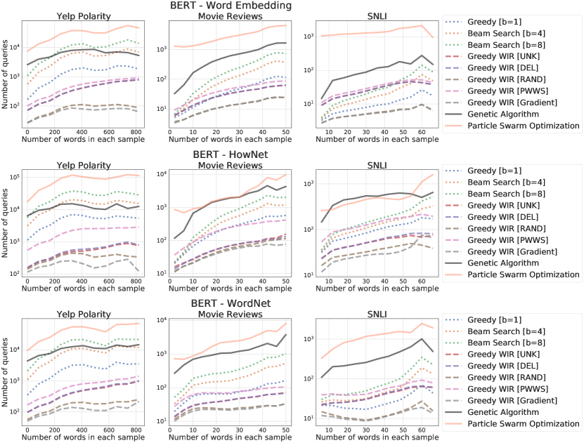
Figure 1: Number of queries vs. length of input text. Similar figure for LSTM models are available in the appendix.

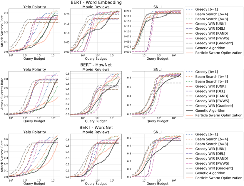
Figure 2: Attack success rate by query budget for each search algorithm and dataset. Similar figure for LSTM models are available in the appendix.

4.1 Attack Success Rate Comparison

Table 6 shows the results of each attack when each search algorithm is allowed to query the victim model an unlimited number of times. Word importance ranking methods makes far fewer queries than beam or population-based search, while retaining over 60% of their attack success rate in each case. Beam search (b=8) and PSO are the two most successful search algorithms in every model-dataset combination. However, PSO is more query-intensive. On average, PSO requires 6.3 times more queries than beam search (b=8), but its attack success rate is only on average $1.2\%$ higher than that of beam search (b=8).

4.2 Runtime Analysis

Using number of queries to the victim model as proxy for total runtime, Figure 1 illustrates how the number of words in the input affects runtime for each algorithm. We can empirically confirm that beam and greedy search algorithms scale quadratically with input length, while word importance ranking scales linearly. For shorter datasets, this did not make a significant difference. However, for the longer Yelp dataset, the linear word importance ranking strategies are significantly more query-efficient. These observations match the expected runtimes of the algorithms described in Table 2.

For shorter datasets, genetic and PSO algorithms are significantly more expensive than the other algorithms as the size of population and number of iterations are the dominating factors. Furthermore, PSO is observed to be more expensive than genetic algorithm.

4.3 Performance under Query Budget

In a realistic attack scenario, the attacker must conserve the number of queries made to the model. To see which search method was most query-efficient, we calculated the search methods’ attack success rates under a range of query budgets. Figure 2 shows the attack success rate of each search algorithm as the maximum number of queries permitted to perturb a single sample varies from $0$ to $20,000$ for Yelp dataset and $0$ to $3000$ for MR and SNLI.

For both Yelp and MR datasets, the linear (word importance ranking) methods show relatively high success rates within just a few queries, but are eventually surpassed by the slower, quadratic methods (greedy and beam search). The genetic algorithm and PSO lag behind. For SNLI, we see exceptions as the initial queries that linear methods make to determine word importance ranking does not pay off as other algorithms appear more efficient with their queries. This shows that the most effective search method depends on both on the attacker’s query budget and the victim model. An attacker with a small query budget may prefer a linear method, but an attacker with a larger query budget may aim to choose a quadratic method to make more queries in exchange for a higher success rate.

Lastly, we can see that both Gradient and RAND ranking methods are initially more successful than UNK and DEL methods, which is due to the overhead involved in calculating word importance ranking for UNK and DEL – for both methods, each attack makes $W$ queries to determine the importance of each word. Still, UNK and DEL outperform RAND at all but the smallest query budgets, indicating that the order in which words are swapped do matter. Furthermore, in 12 out 15 scenarios, UNK and DEL methods perform as well as or even better than Gradient method, which shows that they are excellent substitutes to the Gradient method for black-box attacks.

4.4 Quality of Adversarial Examples

We selected adversarial examples whose original text ${\mathbf{x}}$ was successfully attacked by all search algorithms for quality evaluation. Full results of quality evaluation are shown in Table 4 in the appendix. We can see that beam search algorithms consistently perturb the lowest percentage of words. Furthermore, we see that a fewer number of words perturbed generally corresponds with higher average USE similarity between ${\mathbf{x}}$ and ${\mathbf{x}}_{adv}$ and a smaller increase in perplexity. This indicates that the beam search algorithms generate higher-quality adversarial examples than other search algorithms.

5 Discussion

5.1 How to Choose A Search Algorithm

Across all nine scenarios, we can see that choice of search algorithm can have a modest impact on the attack success rate. Query-hungry algorithms such as beam search, genetic algorithm, and PSO perform better than fast WIR methods. Out of the WIR methods, PWWS performs significantly better than UNK and DEL methods. In every case, we see a clear trade-off of performance versus speed.

With this in mind, one might wonder about what the best way is to choose a suitable search algorithm. The main factor to consider is the length of the input text. If the input texts are short (e.g. sentence or two), beam search is certainly the appropriate choice: it can achieve a high success rate without sacrificing too much speed. However, when the input text is longer than a few sentences, WIR methods are the most practical choice. If one wishes for the best performance on longer inputs regardless of efficiency, beam search and PSO are the top choices.

5.2 Effectiveness of PWWS Word Importance Ranking

Across all tasks, the UNK and DEL methods perform about equivalently, while PWWS performs significantly better than UNK and DEL. In fact, PWWS performs better than greedy search in two cases. However, this gain in performance does come at a cost: PWWS makes far larger number of queries to the victim model to determine the word importance ranking. Out of the 15 experiments, PWWS makes more queries than greedy search in 8 of them. Yet, on average, greedy search outperforms PWWS by $2.5\%$.

Our results question the utility of the PWWS search method. PWWS neither offers the performance that is competitive when compared to greedy search nor the query efficiency that is competitive when compared to UNK or DEL.

5.3 Effectiveness of Genetic Algorithm

The genetic algorithm proposed by Alzantot et al. (2018) uses more queries than the greedy-based beam search (b=8) in 11 of the 15 scenarios, but only achieves a higher attack success rate in 1 scenario. Thus it is generally strictly worse than the simpler beam search (b=8), achieving a lower success rate at a higher cost.

6 Conclusion

The goal of this paper is not to introduce a new method, but to make empirical analysis towards understanding how search algorithms from recent studies contribute in generating natural language adversarial examples. We evaluated six search algorithms on BERT-base and LSTM models fine-tuned on three datasets. Our results show that when runtime is not a concern, the best-performing methods are beam search and particle swarm optimization. If runtime is of concern, greedy with word importance ranking is the preferable method. We hope that our findings will set a new standard for the reproducibility and evaluation of search algorithms for NLP adversarial examples.

Acknowledgements on Funding:

This work was partly supported by the National Science Foundation CCF-1900676. Any Opinions, findings and conclusions or recommendations expressed in this material are those of the author(s) and do not necessarily reflect those of the National Science Foundation.

Appendix A Appendix on Results

A.1 Search Space Choices

Here, we provide more detail about our search space choices.

A.1.1 Transformations

We consider three different ways of generating substitute words:

1. Counter-fitted GLOVE word embedding Mrksic et al. (2016): For a given word, we take its top $N$ nearest neighbors in the embedding space as its synonyms.

2. HowNet Dong et al. (2010): HowNet is a knowledge base of sememes in both Chinese and English.

3. WordNet Miller (1995): WordNet is a lexical database that contains knowledge about and relationships between English words, including synonyms.

A.1.2 Constraints

To preserve grammaticality, we require that the two words being swapped have the same part-of-speech (POS). This is determined by a part-of-speech tagger provided by Flair Akbik et al. (2018), an open-source NLP library.

To preserve semantics, we consider three different constraints:

1. Minimum cosine similarity of word embeddings: For the word embedding transformation, we require the cosine similarity of the embeddings of the two words meet a minimum threshold.

2. Minimum BERTScore Zhang* et al. (2020): We require that the F1 BERTScore between $x$ and $x^{\prime}$ meet some minimum threshold value.

3. Universal Sentence Encoder Cer et al. (2018): We require that the angular similarity between the sentence embeddings of $x$ and $x^{\prime}$ meet some minimum threshold.

For word embedding similarity, BERTScore, and USE similarity, we need to set the minimum threshold value. We set all three values to be $0.9$ based on the observation reported by Morris et al. (2020b) that high threshold values encourages strong semantic similarity. We do not apply word embedding similarity constraint for HowNet and WordNet transformations because it is not guaranteed that we can map the substitute words generated from the two sources to a word embedding space. We can also assume that the substitute words are semantically similar to the original words since they originate from a curated knowledge base.

Lastly, for all attacks carried out, we do not allow perturbing a word that has already been perturbed and we do not perturbed pre-defined stop words.

A.1.3 Datasets

We compare search algorithms on three datasets: the Movie Review and Yelp Polarity sentiment classification datasets and the SNLI entailment dataset. Figure 3 shows a histogram of the number of words in inputs from each dataset. We can see that inputs from Yelp are generally much longer than inputs from MR or SNLI.

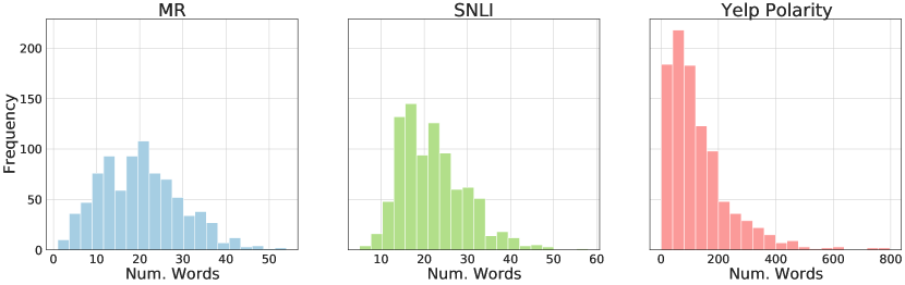
Figure 3: Histogram of words per dataset. Yelp inputs are generally much longer than inputs from MR or SNLI.

A.2 Pseudocode for Search Algorithms

Before presenting the pseudocode of each search algorithm, we define a subroutine called $perturb$ that takes text $x$ and index $i$ to produce set of perturbation $x^{\prime}$ that satisfies the constraints. More specifically, $perturb$ is defined as following:

$$perturb(x,i)=\\ \{T(x,i)\;|\;C_{j}(T(x,i))\;\forall j\in\{1,...,m\}\}$$

where $T({\mathbf{x}},i)$ represents the transformation method that swaps the $i^{th}$ word $x_{i}$ with its synonym to produce perturbed text${\mathbf{x}}^{\prime}$. $C_{1},\dots,C_{m}$ are constraints represented as Boolean functions. $C_{i}(x)=True$ means that text $x$ satisfies constraint $C_{i}$.

Also, $score(x)$ is the heuristic scoring function that was defined in the section 3.2.

Algorithm 1 Beam Search with beam width $b$

Original text $x=(x_{1},x_{2},...x_{n})$

Adversarial text $x_{adv}$ if found

$best$ $\leftarrow$ $\{x\}$

while $best==\emptyset$ do

5:     $X_{cand}$ $\leftarrow$ $\emptyset$

     for all $x_{b}\in best$ do

         for all $i\in\{1,\dots,n\}$ do

              $X_{cand}$ $\leftarrow$ $X_{cand}\cup perturb(x_{b},i)$

         end for

10:     end for

     if $X_{cand}\neq\emptyset$ then

         $x^{*}$ $\leftarrow$ $\operatorname*{arg\,max}_{x^{\prime}\in X_{cand}}{score(x^{\prime})}$

         if $x^{*}$ fools the model then

              return $x^{*}$ as $x_{adv}$

15:         else

              $best$ $\leftarrow$ $\{\text{top }b$ elements of $X_{cand}\}$

$\triangleright$ elements are ranked by their $score$

         end if

     else

20:         End search

     end if

end while

Algorithm 2 Greedy Search

Original text $x=(x_{1},x_{2},...x_{n})$

Adversarial text $x_{adv}$ if found

$x^{*}$ $\leftarrow$ $x$

while $x_{adv}$ not found do

5:     $X_{cand}$ $\leftarrow$ $\emptyset$

     for all $i\in\{1,\dots,n\}$ do

         $X_{cand}$ $\leftarrow$ $X_{cand}\cup perturb(x^{*},i)$

     end for

     if $X_{cand}\neq\emptyset$ then

10:         $x^{*}$ $\leftarrow$ $\operatorname*{arg\,max}_{x^{\prime}\in X_{cand}}{score(x^{\prime})}$

         if $x^{*}$ fools the model then

              return $x^{*}$ as $x_{adv}$

         end if

     else

15:         End search

     end if

end while

Greedy search with word importance ranking requires subroutine for determining the importance of each word in text $x$. We leave the details of the importance functions to be found in individual papers that have proposed them, including Gao et al. (2018), Jin et al. (2019), Ren et al. (2019).

Algorithm 3 Greedy Search with Word Importance Ranking

Original text $x=(x_{1},x_{2},...x_{n})$

Adversarial text $x_{adv}$ if found

$R$ $\leftarrow$ ranking $r_{1},\dots,r_{n}$ of words $x_{1},\dots,x_{n}$ by their importance

$x^{*}$ $\leftarrow$ $x$

5:for $i=r_{1},r_{2},\dots,r_{n}$ in $R$  do

     $X_{cand}$ $\leftarrow$ $perturb(x^{*},i)$

     if $X_{cand}\neq\emptyset$ then

         $x^{*}$ $\leftarrow$ $\operatorname*{arg\,max}_{x^{\prime}\in X_{cand}}{score(x^{\prime})}$

         if $x^{*}$ fools the model then

10:              return $x^{*}$ as $x_{adv}$

         end if

     else

         End search

     end if

15:end for

In genetic algorithm, each population member represents a distinct text produced via $perturb$ and $crossover$ operations. Genetic algorithm has a subroutine called $sample$ that takes in population member $p$ and randomly samples a word to transform with probabilities proportional to the number of synonyms a word has. Also, we modified the $crossover$ subroutine proposed by Alzantot et al. (2018) to check if child produced by $crossover$ operation passes constraints. If the child fails any of the constraints, we retry the crossover for at max 20 times. If that also fails to produce a child that passes constraints, we randomly choose one its parents to be the child with equal probability.

Algorithm 4 Genetic Algorithm (with population size $K$ and generation $G$)

Original text $x=(x_{1},x_{2},...x_{n})$

Adversarial text $x_{adv}$ if found

for $k=1,\dots,K$ do

     $i$ $\leftarrow$ $sample(x)$

5:     $X_{cand}$ $\leftarrow$ $perturb(x,i)$

     $P^{0}_{k}$ $\leftarrow$ $\operatorname*{arg\,max}_{x^{\prime}\in X_{cand}}{score(x^{\prime})}$

end for

for $g=1,\dots,G$ generations do

     for $k=1,\dots,K$ do

10:         $S^{g-1}_{k}$ $\leftarrow$ $score(P^{g-1}_{k})$

     end for

     $x^{*}$ $\leftarrow$ $P^{g-1}_{\operatorname*{arg\,max}_{j}{S^{g-1}_{j}}}$

     if $x^{*}$ fools the model then

         return $x^{*}$ as $x_{adv}$

15:     else

         $P^{g}_{1}$ $\leftarrow$ $x^{*}$

         $p=Normalize(S^{g-1})$

         for $k=2,\dots,K$ do

              $par_{1}\sim P^{g-1}$ with prob $p$

20:              $par_{2}\sim P^{g-1}$ with prob $p$

              $child$ $\leftarrow$ $crossover(par_{1},par_{2})$

              $i$ $\leftarrow$ $sample(child)$

              $X_{cand}$ $\leftarrow$ $perturb(child,i)$

              $P^{g}_{k}$ $\leftarrow$ $\operatorname*{arg\,max}_{x^{\prime}\in X_{cand}}{score(x^{\prime})}$

25:         end for

     end if

end for

Lastly, we leave out the pseudocode for PSO due to its complexity. More detail can be found in Zang et al. (2020).

A.3 Analysis of Attacks against LSTM Models

Figures 4 shows how the number of words in the input affects runtime for each algorithm against LSTM models. Figure 5 shows the attack success rate of each search algorithm as the maximum number of queries permitted to perturb a single sample varies from $0$ to $20,000$ for Yelp dataset and $0$ to $3000$ for MR and SNLI.

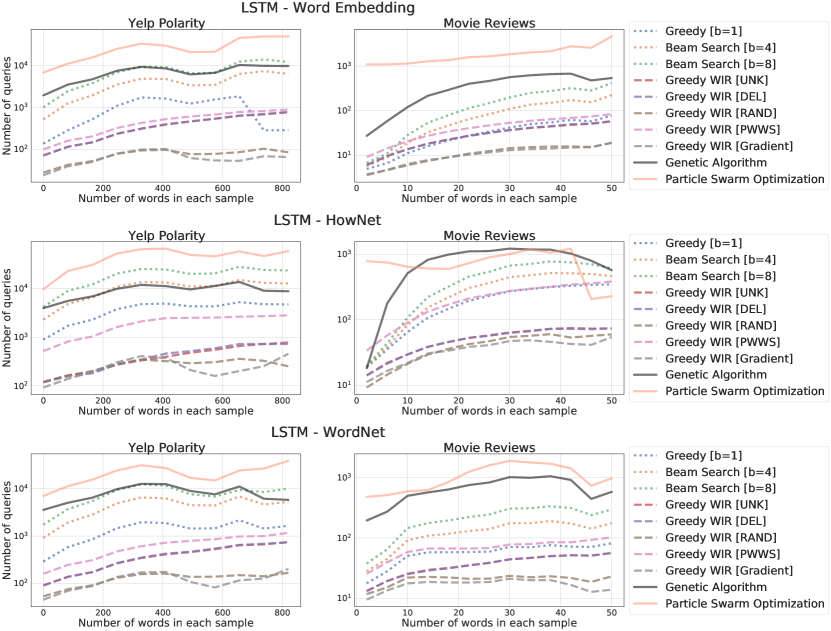
Figure 4: Number of queries vs. length of input text.

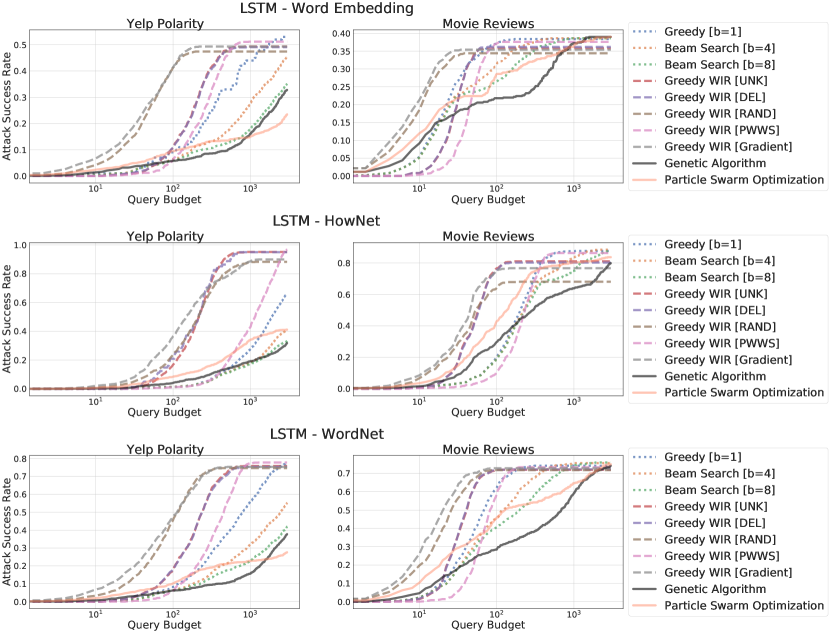
Figure 5: Attack success rate by query budget for each search algorithm and dataset.

A.4 Evaluation of Adversarial Examples

Table 4 shows the average percentage of words perturbed, average Universal Sentence Encoder similarity score, and average percent change in perplexity for all experiments.

Model	Dataset	Search Method	GLOVE Word Embedding			HowNet			WordNet
			Avg P.W. %	Avg USE Sim	$\Delta\%$ Perplexity	Avg P.W. %	Avg USE Sim	$\Delta\%$ Perplexity	Avg P.W. %	Avg USE Sim	$\Delta\%$ Perplexity
BERT	Yelp	Greedy (b=1)	3.41	0.948	21.5	2.52	0.945	22.8	4.76	0.943	49.9
		Beam Search (b=4)	3.26	0.949	20.7	2.45	0.946	22.0	4.49	0.944	46.7
		Beam Search (b=8)	3.20	0.950	20.1	2.42	0.947	21.4	4.46	0.945	46.4
		WIR (UNK)	6.48	0.930	43.5	4.73	0.922	42.3	9.02	0.924	92.1
		WIR (DEL)	6.85	0.928	47.2	5.10	0.919	46.4	9.38	0.923	98.8
		WIR (PWWS)	4.36	0.942	27.3	3.11	0.94	28.1	6.10	0.937	66.1
		WIR (Gradient)	6.16	0.933	37.8	5.58	0.913	44.5	9.10	0.925	86.4
		WIR (RAND)	8.18	0.920	59.1	7.46	0.898	74.6	11.16	0.914	124.8
		Genetic Algorithm	5.06	0.936	33.9	4.21	0.928	42.7	6.70	0.932	77.3
		PSO	6.61	0.929	47.3	6.08	0.913	62.3	9.67	0.922	111.0
	MR	Greedy (b=1)	7.25	0.900	31.8	6.14	0.887	36.5	10.26	0.864	102.8
		Beam Search (b=4)	7.22	0.901	31.4	6.10	0.887	36.1	10.10	0.866	97.9
		Beam Search (b=8)	7.22	0.901	31.4	6.10	0.887	36.1	10.05	0.866	101.6
		WIR (UNK)	9.42	0.884	42.3	7.77	0.866	48.0	14.14	0.845	141.2
		WIR (DEL)	9.62	0.882	46.4	7.69	0.865	46.1	14.60	0.840	146.4
		WIR (PWWS)	7.36	0.898	33.8	6.22	0.884	37.6	10.80	0.865	111.1
		WIR (Gradient)	8.61	0.892	38.1	8.25	0.862	40.8	14.58	0.844	123.2
		WIR (RAND)	10.1	0.881	51.4	9.93	0.846	69.5	17.28	0.827	149.4
		Genetic Algorithm	8.18	0.895	35.8	6.41	0.885	37.8	12.30	0.854	124.5
		PSO	8.71	0.894	39.0	6.46	0.884	38.7	16.08	0.839	187.8
	SNLI	Greedy (b=1)	5.59	0.915	37.8	5.02	0.889	31.7	6.53	0.903	55.9
		Beam Search (b=4)	5.59	0.916	37.8	5.02	0.889	31.6	6.50	0.903	55.7
		Beam Search (b=8)	5.59	0.916	37.8	5.02	0.889	31.6	6.50	0.903	55.9
		WIR (UNK)	6.56	0.911	42.8	5.65	0.887	33.4	8.03	0.899	65.5
		WIR (DEL)	6.77	0.91	44.0	5.81	0.887	34.2	8.22	0.898	67.6
		WIR (PWWS)	5.63	0.915	37.8	5.05	0.89	30.5	6.59	0.906	54.5
		WIR (Gradient)	6.57	0.911	41.6	5.9	0.881	37.7	8.06	0.899	65.1
		WIR (RAND)	7.06	0.909	47.7	6.19	0.884	42.9	8.65	0.895	74.6
		Genetic Algorithm	5.71	0.915	38.5	5.14	0.888	32.7	6.73	0.902	58.3
		PSO	5.76	0.915	38.6	5.14	0.888	32.5	6.94	0.902	58.5
LSTM	Yelp	Greedy (b=1)	4.04	0.943	28.9	2.47	0.948	23.9	4.58	0.946	52.1
		Beam Search (b=4)	4.01	0.942	28.9	2.47	0.949	23.7	4.53	0.946	51.9
		Beam Search (b=8)	4.01	0.943	28.7	2.44	0.949	23.0	4.51	0.946	51.3
		WIR (UNK)	5.83	0.933	42.4	3.51	0.935	34.4	7.22	0.935	75.6
		WIR (DEL)	5.86	0.932	41.1	3.61	0.936	33.3	7.22	0.935	75.4
		WIR (PWWS)	4.57	0.940	32.6	2.58	0.947	23.9	5.14	0.944	57.0
		WIR (Gradient)	7.05	0.926	52.2	5.25	0.916	50.7	8.42	0.929	87.9
		WIR (RAND)	7.28	0.925	53.6	6.33	0.906	69.5	9.40	0.925	102.4
		Genetic Algorithm	5.94	0.933	42.8	3.73	0.930	41.9	6.37	0.936	80.9
		PSO	6.70	0.929	47.3	5.03	0.924	58.7	7.98	0.93	95.2
	MR	Greedy (b=1)	7.19	0.899	33.5	5.96	0.884	37.2	10.21	0.871	100.6
		Beam Search (b=4)	7.19	0.899	33.7	5.96	0.884	37.6	10.03	0.871	98.7
		Beam Search (b=8)	7.19	0.899	34.0	5.96	0.884	37.6	10.00	0.871	97.4
		WIR (UNK)	8.99	0.889	41.7	7.22	0.874	42.9	12.99	0.856	104.5
		WIR (DEL)	9.17	0.889	44.5	7.21	0.874	42.2	13.03	0.856	107.5
		WIR (PWWS)	7.45	0.898	33.7	6.01	0.884	37.1	10.50	0.871	87.9
		WIR (Gradient)	8.73	0.892	41.4	7.33	0.870	40.8	13.12	0.859	104.1
		WIR (RAND)	10.60	0.880	54.0	9.31	0.853	57.7	16.05	0.842	148.2
		Genetic Algorithm	8.02	0.896	36.4	6.36	0.881	39.5	11.98	0.860	120.2
		PSO	8.41	0.893	40.2	6.32	0.882	40.8	13.90	0.854	130.0

Table 4: Quality evaluation of the adversarial examples produced by each search algorithm. ”Avg P.W. %” means average percentage of words perturbed, ”Avg USE Sim” means average USE angular similarity, and ”$\Delta\%$ Perplexity” means percent change in perplexities.

Appendix B Future Work

Submodularity of transformer models.

As mentioned in Section 5, our findings indicate that the NLP attack problem may be approximately submodular when dealing with transformer models. In the image space, attacks designed to take advantage of submodularity have achieved high query efficiency Moon et al. (2019). With the exception of Lei et al. (2019), attacks in NLP are yet to take advantage of this submodular property.

Transformations beyond word-level.

Most proposed adversarial attacks in NLP focus on making substitutions at the word level or the character level. A few works have considered replacing phrases Ribeiro et al. (2018) as well as paraphrasing full sentences Lei et al. (2019); Iyyer et al. (2018). However, neither of these scenarios has been studied extensively. Future work in NLP adversarial examples would benefit from further exploration of phrase and sentence-level transformations.

Motivations for generating NLP adversarial examples.

One purpose of generating adversarial examples for NLP systems is to improve the systems. Much work has focused on improvements in intrinsic evaluation metrics like achieving higher attack success rate via an improved search method. To advance the field, future researchers might focus more on using adversarial examples in NLP to build better NLP systems.

References

- Akbik et al. (2018) Alan Akbik, Duncan Blythe, and Roland Vollgraf. 2018. Contextual string embeddings for sequence labeling. In COLING 2018, 27th International Conference on Computational Linguistics, pages 1638–1649.
- Alzantot et al. (2018) Moustafa Alzantot, Yash Sharma, Ahmed Elgohary, Bo-Jhang Ho, Mani Srivastava, and Kai-Wei Chang. 2018. Generating natural language adversarial examples. arXiv preprint arXiv:1804.07998.
- Bowman et al. (2015) Samuel R. Bowman, Gabor Angeli, Christopher Potts, and Christopher D Manning. 2015. A large annotated corpus for learning natural language inference. In Proceedings of the 2015 Conference on Empirical Methods in Natural Language Processing (EMNLP). Association for Computational Linguistics.
- Cer et al. (2018) Daniel Cer, Yinfei Yang, Sheng-yi Kong, Nan Hua, Nicole Limtiaco, Rhomni St. John, Noah Constant, Mario Guajardo-Cespedes, Steve Yuan, Chris Tar, Yun-Hsuan Sung, Brian Strope, and Ray Kurzweil. 2018. Universal sentence encoder. CoRR, abs/1803.11175.
- Chelba et al. (2013) Ciprian Chelba, Tomas Mikolov, Mike Schuster, Qi Ge, Thorsten Brants, and Phillipp Koehn. 2013. One billion word benchmark for measuring progress in statistical language modeling. CoRR, abs/1312.3005.
- Devlin et al. (2018) Jacob Devlin, Ming-Wei Chang, Kenton Lee, and Kristina Toutanova. 2018. BERT: pre-training of deep bidirectional transformers for language understanding. CoRR, abs/1810.04805.
- Dong et al. (2010) Zhendong Dong, Qiang Dong, and Changling Hao. 2010. Hownet and its computation of meaning. In Proceedings of the 23rd International Conference on Computational Linguistics: Demonstrations, COLING ’10, page 53–56, USA. Association for Computational Linguistics.
- Ebrahimi et al. (2017) Javid Ebrahimi, Anyi Rao, Daniel Lowd, and Dejing Dou. 2017. Hotflip: White-box adversarial examples for text classification. In ACL.
- Gao et al. (2018) Ji Gao, Jack Lanchantin, Mary Lou Soffa, and Yanjun Qi. 2018. Black-box generation of adversarial text sequences to evade deep learning classifiers. 2018 IEEE Security and Privacy Workshops (SPW), pages 50–56.
- Goodfellow et al. (2014) Ian J Goodfellow, Jonathon Shlens, and Christian Szegedy. 2014. Explaining and harnessing adversarial examples. arXiv preprint arXiv:1412.6572.
- Iyyer et al. (2018) Mohit Iyyer, John Wieting, Kevin Gimpel, and Luke Zettlemoyer. 2018. Adversarial example generation with syntactically controlled paraphrase networks.
- Jia et al. (2019) Robin Jia, Aditi Raghunathan, Kerem Göksel, and Percy Liang. 2019. Certified robustness to adversarial word substitutions. arXiv preprint arXiv:1909.00986.
- Jin et al. (2019) Di Jin, Zhijing Jin, Joey Tianyi Zhou, and Peter Szolovits. 2019. Is bert really robust? natural language attack on text classification and entailment. ArXiv, abs/1907.11932.
- Lei et al. (2019) Qi Lei, Lingfei Wu, Pin-Yu Chen, Alex Dimakis, Inderjit S. Dhillon, and Michael J Witbrock. 2019. Discrete adversarial attacks and submodular optimization with applications to text classification. In Proceedings of Machine Learning and Systems 2019, pages 146–165.
- Miller (1995) George A. Miller. 1995. Wordnet: A lexical database for english. Commun. ACM, 38(11):39–41.
- Moon et al. (2019) Seungyong Moon, Gaon An, and Hyun Oh Song. 2019. Parsimonious Black-Box adversarial attacks via efficient combinatorial optimization.
- Morris et al. (2020a) John Morris, Eli Lifland, Jin Yong Yoo, and Yanjun Qi. 2020a. TextAttack: A framework for adversarial attacks in natural language processing. ArXiv, abs/2005.05909.
- Morris et al. (2020b) John X. Morris, Eli Lifland, Jack Lanchantin, Yangfeng Ji, and Yanjun Qi. 2020b. Reevaluating adversarial examples in natural language.
- Mrksic et al. (2016) Nikola Mrksic, Diarmuid Ó Séaghdha, Blaise Thomson, Milica Gasic, Lina Maria Rojas-Barahona, Pei hao Su, David Vandyke, Tsung-Hsien Wen, and Steve J. Young. 2016. Counter-fitting word vectors to linguistic constraints. In HLT-NAACL.
- Pang and Lee (2005) Bo Pang and Lillian Lee. 2005. Seeing stars: Exploiting class relationships for sentiment categorization with respect to rating scales. In Proceedings of the 43rd Annual Meeting of the Association for Computational Linguistics (ACL’05), pages 115–124, Ann Arbor, Michigan. Association for Computational Linguistics.
- Radford et al. (2019) Alec Radford, Jeff Wu, Rewon Child, David Luan, Dario Amodei, and Ilya Sutskever. 2019. Language models are unsupervised multitask learners.
- Ren et al. (2019) Shuhuai Ren, Yihe Deng, Kun He, and Wanxiang Che. 2019. Generating natural language adversarial examples through probability weighted word saliency. In Proceedings of the 57th Annual Meeting of the Association for Computational Linguistics, pages 1085–1097, Florence, Italy. Association for Computational Linguistics.
- Ribeiro et al. (2018) Marco Tulio Ribeiro, Sameer Singh, and Carlos Guestrin. 2018. Semantically equivalent adversarial rules for debugging NLP models. pages 856–865.
- Szegedy et al. (2013) Christian Szegedy, Wojciech Zaremba, Ilya Sutskever, Joan Bruna, Dumitru Erhan, Ian Goodfellow, and Rob Fergus. 2013. Intriguing properties of neural networks. arXiv preprint arXiv:1312.6199.
- Wallace et al. (2019) Eric Wallace, Jens Tuyls, Junlin Wang, Sanjay Subramanian, Matt Gardner, and Sameer Singh. 2019. AllenNLP Interpret: A framework for explaining predictions of NLP models. In Empirical Methods in Natural Language Processing.
- Zang et al. (2020) Yuan Zang, Fanchao Qi, Chenghao Yang, Zhiyuan Liu, Meng Zhang, Qun Liu, and Maosong Sun. 2020. Word-level textual adversarial attacking as combinatorial optimization. In Proceedings of the 58th Annual Meeting of the Association for Computational Linguistics, pages 6066–6080, Online. Association for Computational Linguistics.
- Zhang et al. (2019a) Huangzhao Zhang, Hao Zhou, Ning Miao, and Lei Li. 2019a. Generating fluent adversarial examples for natural languages. In Proceedings of the 57th Annual Meeting of the Association for Computational Linguistics, pages 5564–5569, Florence, Italy. Association for Computational Linguistics.
- Zhang* et al. (2020) Tianyi Zhang*, Varsha Kishore*, Felix Wu*, Kilian Q. Weinberger, and Yoav Artzi. 2020. Bertscore: Evaluating text generation with bert. In International Conference on Learning Representations.
- Zhang et al. (2019b) Wei Emma Zhang, Quan Z. Sheng, and Ahoud Abdulrahmn F. Alhazmi. 2019b. Generating textual adversarial examples for deep learning models: A survey. CoRR, abs/1901.06796.
- Zhang et al. (2015) Xiang Zhang, Junbo Zhao, and Yann LeCun. 2015. Character-level convolutional networks for text classification. In C. Cortes, N. D. Lawrence, D. D. Lee, M. Sugiyama, and R. Garnett, editors, Advances in Neural Information Processing Systems 28, pages 649–657. Curran Associates, Inc.