Inferring the gravitational wave memory for binary coalescence events

Abstract

Full, non-linear general relativity predicts a memory effect for gravitational waves. For compact binary coalescence, the total gravitational memory serves as an inferred observable, conceptually on the same footing as the mass and the spin of the final black hole. Given candidate waveforms for any LIGO event, then, one can calculate the posterior probability distribution functions for the total gravitational memory, and use them to compare and contrast the waveforms. In this paper we present these posterior distributions for the binary black hole merger events reported in the first Gravitational Wave Transient Catalog (GWTC-1), using the Phenomenological and Effective-One-Body waveforms. On the whole, the two sets of posterior distributions agree with each other quite well though we find larger discrepancies for the $\ell=2,m=1$ mode of the memory. This signals a possible source of systematic errors that was not captured by the posterior distributions of other inferred observables. Thus, the posterior distributions of various angular modes of total memory can serve as diagnostic tools to further improve the waveforms. Analyses such as this would be valuable especially for future events as the sensitivity of ground based detectors improves, and for LISA which could measure the total gravitational memory directly.

I Introduction

The detection of gravitational waves enables tests of general relativity that were not possible using the electromagnetic window. For example, through observations of compact binary mergers one can verify higher order post-Newtonian effects in the inspiral regime, and probe the nature of the final remnant black hole in the post-merger regime Abbott (2016, 2019a, 2019b). Similarly, in the search for potential deviations from general relativity, one can use the parameterized post-Newtonian formalism as a general framework in the inspiral regime, and black hole perturbation theory in the post-merger regime. The merger itself cannot be addressed by these approximation schemes because non-linear effects of general relativity are especially important there. On the other hand, precisely for the same reason, the merger provides a promising place to look for potential deviations from general relativity.

So far, there is no generally accepted framework for describing the merger itself analogous to the parameterized post-Newtonian framework. Several tests have been proposed in the literature which attempt to probe different aspects of the merger. However, to reliably test whether predictions of general relativity are borne out in observations, one needs to be confident that the theoretical waveforms used in these tests capture predictions of the theory to a sufficiently high degree of accuracy. Although so far, there is no generally accepted framework to test the accuracy of theoretical predictions describing the merger itself, several tests have been proposed in the literature to probe different aspects of these predictions. These include, for example, various consistency checks between the inspiral and the merger Ghosh et al. (2018); Cabero et al. (2018), and also tests of phenomenological waveform models for the merger Abbott (2016). In this paper we suggest that the total gravitational memory can be used as a new tool in the same direction.

General relativity predicts that memory associated with gravitational waves emitted in compact binary coalescences would be generically non-zero. For the interferometric gravitational wave detectors, this corresponds to a permanent displacement of the test masses due to the flux of gravitational waves across the plane of the detector Christodoulou (1991); Frauendiener (1992); Thorne (1992); Blanchet and Damour (1992); Wiseman and Will (1991). See also Johnson et al. (2019); Kennefick (1994); Favata (2008, 2009a, 2009b, 2010, 2011) for later work discussing prospects for detecting memory and further calculations of the memory within the post-Newtonian framework. Advances in numerical relativity towards calculating memory in numerical simulations of black hole mergers are given in Pollney and Reisswig (2011); Mitman et al. (2020). A direct measurement of the memory would be a probe of non-linear aspects of general relativity, and also of the merger, since the effect is the largest during this phase. However, thus far, we do not have a direct measurement either for single events, or collectively for a population of events Hübner et al. (2020); Divakarla et al. (2020); Talbot et al. (2018); McNeill et al. (2017); Lasky et al. (2016). But the total gravitational memory is a bonafide observable in full general relativity, expressible as a functional of the gravitational wave strain in a detector. Therefore, assuming general relativity, it is possible to infer its value.

As we now explain, this inference relies on the waveform model used. For a binary system, a gravitational waveform received at a detector is parameterized by at least 10 intrinsic parameters (without restricting oneself to general relativity): the two component masses $m_{1}$ and $m_{2}$, the individual spins of the two components $\mathbf{S}_{1}$ and $\mathbf{S}_{2}$, and two additional parameters in case the system is in an eccentric orbit (namely, the eccentricity and the orientation of the elliptical orbit). The total mass is denoted $M=m_{1}+m_{2}$. It is conventional to use the dimensionless spin parameter $\chi_{i}=\mathbf{S}_{i}\cdot\mathbf{\widehat{L}}/m_{i}^{2}$ ($i=1,2$) instead of the spin itself, where $\mathbf{\widehat{L}}$ is the unit-vector in the direction of the orbital angular momentum vector $\mathbf{L}$. Similarly, the effective spin $\chi_{eff}$ which appears in several waveform models is a weighted sum of the individual spins: $\chi_{eff}=(m_{1}\chi_{1}+m_{2}\chi_{2})/M$. The dimensionless spin components perpendicular to $\mathbf{\widehat{L}}$ are denoted $\chi_{1,2}^{\perp}$. In addition to the masses and spins, we will have 4 extrinsic parameters. This includes the luminosity distance to the source $D_{L}$, and three additional extrinsic parameters which determine the orientation of the source. Let us denote the intrinsic parameters collectively by $\vec{\lambda}$, and the 4 extrinsic parameters by $\vec{\mathcal{A}}$. If one or both of the compact objects is a neutron star, we will have further parameters depending on the structure of the star. Given these parameters, we can determine the gravitational waveforms $h_{+,\times}(t;\vec{\lambda},\vec{\mathcal{A}})$ for the two polarizations. Given, in addition, the orientation of the detector which requires three additional angles collectively denoted $\vec{\Theta}$, the received strain $h(t;\vec{\lambda},\vec{\mathcal{A}},\vec{\Theta})$ in a detector can be calculated by a suitable projection of $h_{+,\times}$. One can show that one of the angles in $\vec{A}$ is degenerate with an angle in $\vec{\Theta}$, namely, the polarization angle (see e.g. Harry and Fairhurst (2011)). Consequently, there are only three independent parameters in $\vec{\mathcal{A}}$: the luminosity distance $D_{L}$, the inclination angle $\iota$ which is the angle between the source axis and the line of sight to the detector, and a phase $\varphi_{0}$. The three parameters in $\vec{\Theta}$ are the sky-location of the source in the detector frame $(\theta,\phi)$, and the polarization angle $\psi$.

Given the measurement of the strain in a detector, one can match the most accurate available model and determine the values or, more precisely, the posterior probability distributions, of the intrinsic parameters $\vec{\lambda}$. These distributions are in fact among the most important results of the observation, providing us with the measured values of these parameters that describe the binary. Note that the above discussion assumes that the wavelength of the signal is much longer than the length of the detector arms, and that the signal duration in much shorter than a sidereal day. Thus the distinction between intrinsic and extrinsic parameters is more complicated for e.g. the LISA detector, but we shall not consider this detail here.

Once we have the probability distribution for $\vec{\lambda}$, assuming general relativity, we can use it to calculate values of other important observables associated with the binary. Following a general convention, we will refer to the values (or rather, the probability distributions) of $\vec{\lambda}$ as measured quantities, and those of additional observables that can then be deduced as inferred values. The most widely used inferred observables for a binary are the mass $M_{f}$, the spin $\mathbf{S}_{f}$ and the recoil (or kick) velocity $\mathbf{v}$ of the remnant. The total gravitational wave memory is on a similar footing as these: given the waveform parameters and a particular waveform model, values of various modes in the angular decomposition of the memory can be uniquely inferred assuming general relativity.

The first goal of this paper is to carry out this procedure in detail and to obtain the posterior distributions of the memory modes for the binary black hole merger events reported in the first Gravitational Wave Transient Catalog (GWTC-1) Abbott et al. (2019a). Now, the properties of the commonly used inferred observables – the final black hole parameters such as $M_{f},\mathbf{S}_{f},\mathbf{v}$– have important astrophysical and theoretical applications. Gravitational memory is likely not of direct astrophysical interest. Nonetheless, since it is a genuine observable in general relativity, it has interesting theoretical implications. In particular, differences in the memory for different waveform models are significant. If for example, for a given event, the memory turns out to be statistically different for different waveform models, they cannot both be accurate approximations to exact general relativity. Therefore the statistical difference would point to a difference between the underlying physical assumptions of the models, indicating that these models can be further improved. As detectors become increasingly sensitive, these differences might become more significant and can play a useful role in improving waveform models. The second goal of this paper, then, is to advocate the use of the memory as a diagnostic tool for investigating physical differences between different waveform models.

The plan for the rest of the paper is the following. In Sec. II we shall explain the basic formalism for calculating the linear and non-linear parts of the memory. Sec. III applies this to the events published by the LIGO and Virgo collaborations and finally Sec. IV concludes with a discussion of the results and possible future applications of the memory.

II Constraints on gravitational waveforms and the memory

We begin with a description of the gravitational wave signal emitted by a compact binary source. The starting point for understanding the behavior of gravitational radiation in numerical relativity and gravitational waveform modeling is the Weyl tensor component $\Psi_{4}=C_{abcd}n^{a}\bar{m}^{b}n^{c}\bar{m}^{d}$. Here $C_{abcd}$ is the Weyl tensor, and $(l^{a},n^{a},m^{a},\bar{m}^{2})$ is a suitably chosen null-tetrad adapted to spheres centered on the source. Thus, $l^{a}$ and $n^{a}$ are respectively the outgoing and ingoing null normals to these spheres, while the complex vector field $m^{a}$ is tangential to the spheres and adapted to the source axis, and $\bar{m}^{a}$ is the complex conjugate of $m^{a}$. The only non-vanishing inner-products are $m\cdot\bar{m}=1$ and $l\cdot n=-1$. The notion of spin-weight plays an important role. This refers to the behavior of quantities under ‘spin rotations’ $m\rightarrow e^{i\psi}m$. A quantity $F$ is said to have spin-weight $s$ if $F\rightarrow e^{is\psi}F$ under this transformation. Thus, $m^{a}$ itself has spin weight $+1$ while $\bar{m}^{a}$ has $s=-1$. The Weyl tensor component $\Psi_{4}$ has $s=-2$.

The two polarizations of the gravitational wave strain $h_{+,\times}$ are related to $\Psi_{4}$ according to

$$\Psi_{4}=-\ddot{\mathfrak{h}}\quad\textrm{where}\quad\mathfrak{h}:=h_{+}-ih_{\times}\,.$$ (1)

The emitted gravitational wave signal at large distances from the source can be expanded in terms of spin-weighted spherical harmonics:

$$\mathfrak{h}=\frac{1}{D_{L}}\,\,\sum_{\ell=2}^{\infty}\sum_{m=-\ell}^{\ell}\mathfrak{h}_{\ell m}(t;\vec{\lambda})\,\,{}_{-2}Y_{\ell m}(\iota,\varphi_{0})\,.$$ (2)

Here ${}_{-2}Y_{\ell m}$ is a spin-weighted spherical harmonic of spin weight $-2$, and $D_{L}$ is the luminosity distance from the source. See e.g. Reisswig and Pollney (2011); Berti et al. (2007) for a discussion of the integrations in time required to go from $\Psi_{4}$ to $\dot{\mathfrak{h}}$ and eventually to $h_{+,\times}$.

As explained in Section I , $h_{+,\times}$ are functions of time, and they are parameterized by $(\vec{\lambda},\iota,\varphi_{0},D_{L})$. The signal $h(t)$ seen at a detector is

$$h(t;\vec{\lambda},\vec{A},\Theta) = F_{+}(\theta,\phi,\psi)h_{+}(t;\vec{\lambda},\vec{A})$$ (3)

$$+ F_{\times}(\theta,\phi,\psi)h_{\times}(t;\vec{\lambda},\vec{A})\,.$$

Here $F_{+,\times}$ are the detector beam pattern functions.

Numerical simulations provide us with the mode amplitudes $h_{\ell m}$ for a selected set of points in parameter space and for a few chosen modes for which $\Psi_{4}$ can be extracted reliably. For analyzing gravitational wave signals, it is much more practical to construct analytical models that interpolate between these chosen points in parameter space, and then use these models for gravitational wave mode amplitudes. Significant advances have been made in addressing this interpolation problem (see e.g. Setyawati et al. (2020) for recent work in this direction). Two particular waveform models have been used extensively for interpreting gravitational wave data. The first is the Effective-One-Body (EOB) framework originally suggested in Buonanno and Damour (1999); see Damour and Nagar (2016) for a review and e.g. Ossokine et al. (2020); Bohé et al. (2017); Taracchini et al. (2014a); Pan et al. (2014a, 2011); Nagar et al. (2018); Damour and Nagar (2014) for further developments. The second commonly used models are the so-called Phenomenological models originally proposed in Ajith et al. (2008); see e.g. Khan et al. (2020, 2019); London et al. (2018); Khan et al. (2016); Husa et al. (2016); Santamaria et al. (2010) for further developments. It is beyond the scope of this article to review the basic ideas underlying these models, comparisons between them, and their relative strengths and weaknesses. Rather, we will use them to perform ‘null tests’ by first assuming that they both correctly capture general relativity, with sufficient accuracy for detection and parameter estimation in binary mergers, and then comparing their predictions for other observables as a diagnostic tool for potential systematic errors.

Our analysis is based on an infinite tower of constraints on gravitational waveforms, imposed by certain ‘balance laws’ in full, non-linear general relativity. Let us begin with the easier cases, namely the balance laws for energy $E$ and linear momentum $P_{i}$. Let us first note that the total fluxes, $\Delta E$ and $\Delta P_{i}$, carried away by the gravitational waves are given by

$$\Delta E = \frac{D_{L}^{2}c^{3}}{16\pi G}\int_{-\infty}^{\infty}\!\!\!dt\,\oint d\Omega\,\,|\dot{\mathfrak{h}}|^{2}\,,$$ (4)

$$\Delta{P}_{i} = \frac{D_{L}^{2}c^{2}}{16\pi G}\int_{-\infty}^{\infty}\!\!\!dt\,\oint d\Omega\,\,\hat{x}_{i}(\iota,\varphi_{0})|\,\dot{\mathfrak{h}}|^{2}\,\,.$$ (5)

Here $\hat{x}_{1}=\sin\iota\cos\varphi_{0}$, $\hat{x}_{2}=\sin\iota\sin\varphi_{0}$, $\hat{x}_{3}=\cos\iota$ and $d\Omega=\sin\iota\,d\iota\,d\varphi_{0}$. Note that the fluxes $\Delta E$ and $\Delta P_{i}$ are completely determined by the waveform $\mathfrak{h}$. Therefore, given the initial (i.e., ADM) mass and the waveform, the balance laws determine the energy-momentum of the final black hole from which one can extract its mass $M_{f}$ and its recoil velocity $\mathbf{v}$.

Now, since the radiated energy, the recoil velocity, and the final mass are all parameters of direct astrophysical interest, there is an extensive literature on calculating these quantities as functions of the initial parameters Healy and Lousto (2017); Varma et al. (2019); Zappa et al. (2018). These functions are typically obtained as fits to the results of numerical simulations. But as indicated above, we can also calculate these quantities using the model waveforms and the initial parameters that label them. If these waveforms are to accurately represent general relativity, the answers must agree with the fits from numerical relativity. Note that it is not obvious that the two calculations must necessarily agree. As an example of the gap between the two calculations, consider the mass $M_{f}$ and the spin $\mathbf{S}_{f}$ of the final black hole. In numerical relativity, these are typically calculated using geometrical fields on black hole horizons rather than waveforms in the asymptotic regions (see e.g. Dreyer et al. (2003); Owen (2009)). While one expects the two sets of values to agree at late times, their equality has not yet been established mathematically (because of technical issues concerning the structure at future timelike infinity $i^{+}$). Therefore, a comparison between the two would serve as a useful check on overall consistency. In addition, as we discuss in Section III.1, one can view such comparisons as accuracy tests for the waveforms. Any disagreements, even if not significant for current gravitational wave data analysis purposes, might point directions leading to improved waveform models. Eventually, as detectors improve in sensitivity, accuracy requirements on the waveforms become more stringent. Thus, such improvements might be part of the various ingredients in waveform modeling necessary in the coming era of high precision gravitational wave astronomy.

The main focus of this paper is on the non-trivial constraints on the waveforms obtained from the fluxes of supermomenta which, as we shall now see, are closely connected with the total gravitational memory, which is given by

$$\Delta\mathfrak{h}(\iota,\varphi_{0})=\left.\mathfrak{h}\right|_{u=\infty}-\left.\mathfrak{h}\right|_{u=-\infty}\,.$$ (6)

In practice, $\mathfrak{h}$ can be calculated by performing two time-integrals of $\Psi_{4}$. This procedure involves two integration constants Reisswig and Pollney (2011); Berti et al. (2007). The first vanishes in binary coalescences, since the Bondi news $\dot{\mathfrak{h}}$ goes to zero in the distant past as well as distant future (just as $\Psi_{4}$ does). The second is generally used to set $\mathfrak{h}|_{u=-\infty}\,=0$. However, since the total memory $\Delta\mathfrak{h}$ is a difference, its value is independent of the choice of this integration constant; it is a well-defined observable in general relativity, without any further inputs.

The value of $\Delta\mathfrak{h}$ is governed by the supermomentum balance laws, associated with supertranslations. More precisely, presence of gravitational waves in the asymptotic region forces one to enlarge the 4 dimensional group of translations of flat space-time to an infinite dimensional group of “angle dependent translations”, called supertranslations Bondi et al. (1962); Sachs (1962). Just as there are energy momentum balance laws associated with asymptotic translations, Einstein’s equations imply that there are supermomentum balance laws associated with supertranslations Ashtekar and Streubel (1981). As shown in Ashtekar et al. (2019), under assumptions that are normally made in the analysis of compact binary coalescence, they imply:

$$\eth^{2}\Delta\mathfrak{h} = -\frac{2G}{D_{L}c^{2}}\Big{(}M-\frac{M_{f}}{\gamma^{3}(1-\mathbf{v}\cdot\hat{x}/c)^{3}}\Big{)}$$ (7)

$$+ \frac{D_{L}}{2c}\int_{-\infty}^{\infty}\!\!\!dt|\dot{\mathfrak{h}}|^{2}\!\,.$$

Here, $M$ is the total initial mass of the system; $M_{f}$, the mass of the final black hole; $\mathbf{v}$, the recoil velocity; and, $\eth$, the angular derivative, whose action on a scalar $F$ with spin weight $s$ is a spin weight $s+1$ scalar, given by Gelfand et al. (1963); Goldberg et al. (1967)

$$\eth F:=-\frac{1}{\sqrt{2}}(\sin\iota)^{s}\left(\frac{\partial}{\partial\iota}+\frac{i}{\sin\iota}\frac{\partial}{\partial\varphi_{0}}\right)\left(\frac{F}{(\sin\iota)^{s}}\right)\,.$$ (8)

Since $\Delta\mathfrak{h}$ is the strain, it has spin weight $-2$. Thus, the left-hand-side of Eq. (7) has spin-weight 0, consistent with the right-hand-side.

Note that both sides of Eq. (7) have a $(\iota,\varphi_{0})$ dependence. Therefore, we can carry our a mode decomposition of this equation using spherical harmonics

$$C_{\ell}(\Delta\mathfrak{h})_{\ell,m} = -\frac{2G}{D_{L}c^{2}}\Big{(}M\,-\frac{M_{f}}{\gamma^{3}(1-\frac{\mathbf{v}}{c}\cdot\hat{x})^{3}}\Big{)}_{\ell,m}$$ (9)

$$+ \,\frac{D_{L}}{2c}\,\Big{(}\int_{-\infty}^{\infty}\!\!\!dt|\dot{\mathfrak{h}}|^{2}\Big{)}_{\ell,m}$$

where

$$C_{\ell}=\frac{1}{2}\,(\ell-1)\ell(\ell+1)(\ell+2)\,.$$ (10)

The $\ell=0$ and $\ell=1$ components of (9) provide us the balance laws for energy and momentum. (Note that $C_{\ell}=0$ in these cases.) Now, as we remarked above, if we know the initial mass $M$, expressions (4) and (5) of the energy and momentum flux, together with the balance laws (9) for $\ell=0,1$ can be used to determine the mass $M_{f}$ and the recoil velocity of the final black hole. Once $M,M_{f}$ and $\mathbf{v}$ are known, the only other field in Eq. (9) is the waveform $\mathfrak{h}$. Therefore, the $\ell\geq 2$ modes of Eq. 9 provides an infinite tower of constraints to be tested on the $\mathfrak{h}$ provided by waveform models.

However, currently the models do not incorporate the total memory $\Delta\mathfrak{h}$ that appears on the left side of (9), whence the constraints are violated for $\ell\geq 2$. But the right hand side is dominated by aspects of the waveform that, one expects, are well modeled. For example the leading contribution to the right hand side comes from the $(2,\pm 2)$ mode of the waveform, which all waveform models incorporate. Hence we can turn around the constraint, and use it to calculate the memory using the well modeled aspects of the waveform. Thus, Eq. (9) serves as the primary equation which determines the total memory and its mode decomposition. (The first term on the right side is often called the “linear” memory and the second term the “non-linear” memory.)

III Inferred memory for the observed events

For the observed events, parameter estimation using EOB and Phenom models provides us with two posterior distributions for the initial parameters. Given either of them and the corresponding waveform, we can calculate the probability distribution of different modes of the memory. We can do this by taking sample points from the posterior, and then using Eq. (9) to calculate the memory for each sample. This would then give us two posterior distributions of the inferred memory for any given event. We can then check if the the differences in the inferred memory between the two models is less than the statistical errors. In all of the following we use the IMRPhenomPv2 and SEOBNRv3 for events published in the GWTC-1 catalog.

The first step in this procedure is to use the energy-momentum flux to calculate the remnant parameters. This procedure provides us with a posterior probability distribution for the mass and the recoil velocity of the final black hole. We carry out this step in Section III.1. In Section III.2, we use these values in conjunction with Eq. (9) to arrive at a streamlined procedure to calculate the inferred values of various angular modes of the memory. In Section III.3 this procedure is used to obtain the probability distributions for the leading memory modes in the GWTC-1 events. Differences between these distributions can be used as diagnostic tools to detect potential discrepancies and further improve the waveforms.

III.1 The remnant mass $M_{f}$ and recoil velocity $\mathbf{v}$

As we discussed in Section II, given a waveform model we can use Eq. (4) and (5) to calculate the remnant mass $M_{f}$ and recoil velocity $\mathbf{v}$. One can then compare these values with the fits to masses and recoil velocities provided by numerical relativity using fields at the horizon Varma et al. (2019) and the posterior probability for the input parameters provided by the model. This comparison provides a first check on the model waveforms. Assuming that each waveform agrees with the corresponding numerical relativity prediction, one can compare the predictions of the two waveform models. As we will see, this comparison can bring out the differences between the models, thereby providing guidance for further improvements. Determination of $M_{f}$ and $\mathbf{v}$ will also serve a second purpose: Knowing their values, we will be able to calculate the $\ell\geq 2$ components of the memory in Section III.2.

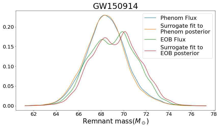
Figure 1: GW150914: distribution of the final mass using the IMRPhenomPv2 and SEOBNRv3 models, compared with the numerical relativity fits applied to each of the posterior distributions. Unlike the kick-velocity results shown in Fig. 3, the results for the final mass using the two models is mostly consistent with the numerical relativity results. The reason is that the energy flux is dominated by the $\ell=2$ modes which are accurately modeled.

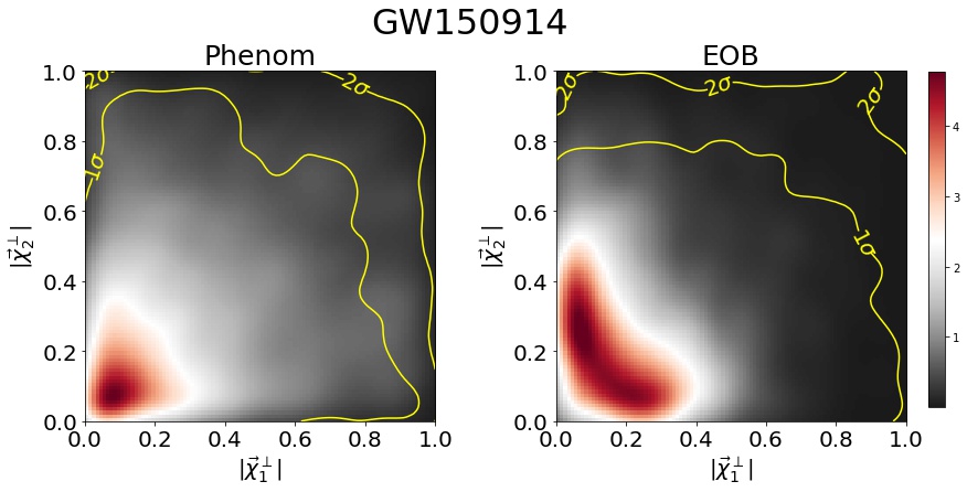
Figure 2: GW150914: Posterior distributions for the perpendicular dimensionless spin components $\chi^{\perp}_{1,2}$. The Phenom model uses a single effective spin while the EOB is parameterized by the individual spins. This gives rise to the bimodal distribution for $\chi_{1,2}^{\perp}$ in the EOB model, which in turn leads to the double hump in the posterior distribution of the final mass in Fig. 1.

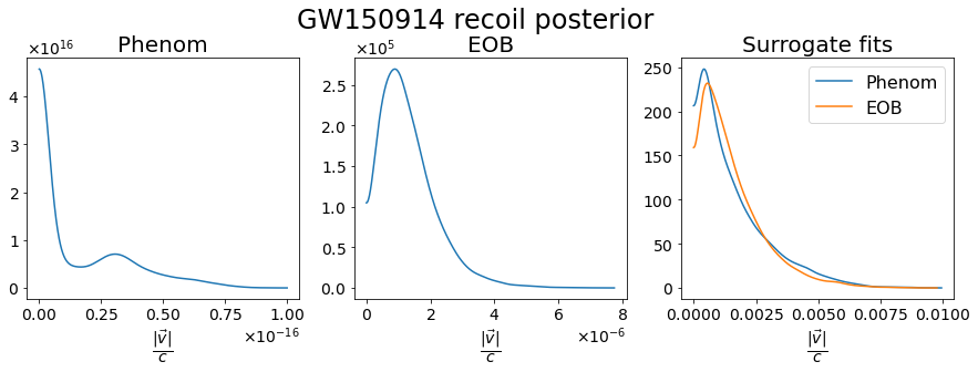
Figure 3: GW150914: Posterior distribution for the recoil velocity (in units with $c=1$) using the IMRPhenomPv2 (left panel) and SEOBNRv3 (middle panel) models, and also accurate fits to numerical relativity calculations (right panel). We note large discrepancies between both the models and the accurate numerical relativity results; the distribution in the left panel has the bulk of its support for $v/c\sim\mathcal{O}(10^{-16})$ (making it consistent with being purely numerical noise), the middle panel for $\mathcal{O}(10^{-6})$, while the correct answer in the right panel has $\mathcal{O}(10^{-3})$. As discussed in the text, this is not surprising because neither of the models attempt to model the higher modes necessary for the kick velocity. However, the discrepancy between the Phenom and EOB models is also interesting to note.

To determine $M_{f}$ and $\mathbf{v}$, we need to use the flux expressions Eq. (4) and (5). However, there is a subtlety: Since waveforms are readily available only for finite time intervals, in practice we have to truncate the time integrals in flux expressions to finite intervals. In the distant future, truncation can be carried out readily without incurring excessive errors because the waveform decays exponentially. However, in the past the flux falls-off slowly. For the Phenom model the waveform is available for sufficiently early times and hence the error due to truncation can be made negligible. However for the EOB model, we are unable to generate the waveform at sufficiently early times; the implementation in the LAL Simulation software library Veitch et al. (2015); LIGO Scientific Collaboration (2018) currently requires the reference frequency and the starting frequency to be identical. The reference frequency –the frequency at which time dependent parameters are quoted– used in the GWTC-1 catalog is 20Hz. It is somewhat more complicated to go to lower frequencies, and we will leave this to future work. While the lower frequencies are unimportant for detection and parameter estimation, their contribution to total radiated energy (4) is not negligible. Therefore, to reduce this truncation error we will add the energy radiated away from 0Hz to 20Hz to 0PN order. This can be calculated analytically using the formula

$$\Delta E_{{\rm 0PN}}=M\,\frac{\nu}{2}\,(\pi GMf_{\rm start})^{2/3}$$ (11)

which describes the 0PN radiated energy $\Delta E_{{\rm 0PN}}$ from retarded time $-\infty$ to when the system reaches a frequency of $f_{\rm start}$. Here $\nu=m_{1}m_{2}/M^{2}$ is the symmetric mass ratio. Using this procedure, for each of the two models we can calculate the remnant parameters in two different ways: (i) using the energy and momentum fluxes for each waveform model, and, (ii) using the numerical relativity fits on the posterior distribution of the input parameters, as determined from the respective model. Adding (11) significantly improves the agreement between final mass calculated from EOB flux and the fits.

This procedure was carried out for all events considered in this paper. Fig. 1 illustrates the results with the posterior distribution of $M_{f}$ in the case of GW150914. This is based on the posterior samples available in the GWTC-1 catalog Abbott et al. (2019a), for both the IMRPhenomPv2 and SEOBNRV3 waveform models; these are all described in further detail in Sec. III.3.

For each model, there is an excellent match between (i) the final mass as calculated from the flux and (ii) the NR fits from same posteriors. However there is a slight disagreement between the two models. Although it is not statistically significant, there is an interesting qualitative difference: While the Phenom plots are a near-Gaussian, the EOB plots show a ‘double hump’. The origin of this difference lies in the differences in parameter estimation of the 2 models, particularly in the way precession is treated. This can be seen in Fig. 2 which shows the posterior distributions of the two components of the dimensionless spins, perpendicular to the orbital angular momentum. The source of the bimodality of the EOB final mass can be traced back to that in this posterior distribution which also shows two modes. Taking samples from each mode in Fig. 2 and comparing with the corresponding points for the EOB distribution in Fig. 1 reveals that the peaks in each of these distributions are correlated. The bottom right peak in Fig. 2 corresponds to the higher peak in Fig. 1, while the top left peak in Fig. 2 correspnds to the lower peak in Fig. 1. In the Phenom model on the other hand, the double hump is absent both in the posterior of spin distributions and the posterior distribution of the inferred $M_{f}$. These differences are all within $1\sigma$ of the distributions, and therefore they are not statistically significant. However this points to differences that might become significant with even louder events that we are likely to see as the sensitivity of the detectors increases.

The recoil velocity $\mathbf{v}$, on the other hand, shows completely different behavior in each model depending on whether it is calculated using (i) the momentum flux, or (ii) using numerical fits. In addition, the values predicted in the two models using momentum flux are also quite different as seen in Fig. 3. While the kicks from the flux of Phenom are below numerical precision, in EOB the norm of the kick is: $v/c\,\sim 10^{-6}$. The NR fits, by contrast, yield a much larger kick, $v/c\,~{}10^{-3}$. However, the disagreement between the models and NR is not surprising because neither model contains the ‘higher modes’ that are important for calculating the kick. Fortunately, for calculation of memory $(\Delta\mathfrak{h})_{\ell m}$ in Section III.2, this discrepancy does not play a role because even with a recoil velocity $v/c\,\sim 10^{-3}$, the first term on the right hand side of (9) that contains the recoil velocity is negligible compared to the second term. For definiteness, we will present all results using the recoil velocity as calculated by the fluxes of the waveform model being used.

III.2 Memory

For an elliptically polarized gravitational wave one can choose a frame (aligned with the principal polarization axes) in the plane transverse to the direction of propagation such that $h_{+,\times}$ are given by

$$h_{+} = \eta(t)\left(\frac{1+\cos^{2}\iota}{2}\right)\cos(2\varphi_{0}+2\varphi(t))\,,$$ (12)

$$h_{+} = \eta(t)\cos\iota\sin(2\varphi_{0}+2\varphi(t))\,.$$ (13)

Here $\eta(t)$ is a slowly varying amplitude, $\varphi(t)$ is the orbital phase, and $\varphi_{0}$ is an initial phase. Before we apply the described procedure to get the distribution of memory generally, consider the simple case of an absence of precession and higher modes. The waveform is dominated by the $\ell=2,m=\pm 2$ modes. In this case, the complex combination $\mathfrak{h}=h_{+}-ih_{\times}$ is given by a combination of the $(2,\pm 2)$ spin-weighted spherical harmonics:

$$\mathfrak{h} = e^{2i\varphi_{0}}\frac{(1+\chi)^{2}}{4}\mathfrak{h}_{0}(t)+e^{-2i\varphi_{0}}\frac{(1-\chi)^{2}}{4}\mathfrak{h}^{\star}_{0}(t)$$ (14)

$$\propto {}_{-2}Y_{2,2}(\iota,\varphi_{0})\mathfrak{h}_{0}(t)+{}_{-2}Y_{2,-2}(\iota,\varphi_{0})\mathfrak{h}^{\star}_{0}(t)\,.$$

where $\mathfrak{h}_{0}=\eta(t)e^{-2i\varphi(t)}$ and $\chi:=\cos\iota$. When we calculate $|\dot{\mathfrak{h}}|^{2}$ in the right hand side of Eq. (9), we will obtain products of ${}_{2}Y_{2,\pm 2}$ which can be expanded in terms of the standard spherical harmonics including in particular $Y_{20}(\iota,\varphi_{0})$ and $Y_{40}(\iota,\varphi_{0})$. Since the original waveform model does not include these modes, the model waveform does not satisfy Eq. (9) and therefore it is not consistent with general relativity. To address this situation, an obvious approach is to modify the waveform model by adding these specific memory modes. This process can be continued iteratively and will converge. In practice, as we shall shortly discuss, the first iteration will suffice and we shall not consider higher iterations in this paper.

The same procedure works for a more general model consisting of higher modes. In general, given that $|\dot{\mathfrak{h}}|^{2}$ has spin weight 0, it can be expanded as

$$|\dot{\mathfrak{h}}|^{2}=\sum_{\ell=0}^{\infty}\sum_{m=-\ell}^{\ell}\alpha_{\ell m}Y_{\ell m}(\iota,\varphi_{0})\,.$$ (15)

The coefficients $\alpha_{\ell m}$ appearing in this expansion can be written in terms of the $3j$-symbols as

$$\alpha_{\ell m} = \sum_{\ell_{1},\ell_{2}=2}^{\infty}\sum_{m_{1}=-\ell_{1}}^{\ell_{1}}\sum_{m_{2}=-\ell_{2}}^{\ell_{2}}\mathfrak{h}_{\ell_{1},m_{1}}\mathfrak{h}_{\ell_{2},m_{2}}^{\star}\oint{}_{-2}Y_{\ell_{1}m_{1}}(\iota,\varphi_{0}){}_{-2}Y_{\ell_{2}m_{2}}^{\star}(\iota,\varphi_{0})Y_{\ell m}^{\star}(\iota,\varphi_{0})\,d\Omega$$ (16)

$$= \sum_{\ell_{1},\ell_{2}=2}^{\infty}\sum_{m_{1}=-\ell_{1}}^{\ell_{1}}\sum_{m_{2}=-\ell_{2}}^{\ell_{2}}\mathfrak{h}_{\ell_{1},m_{1}}\mathfrak{h}_{\ell_{2},m_{2}}^{\star}(-1)^{m+m_{2}}\sqrt{\frac{(2\ell_{1}+1)(2\ell_{2}+1)(2\ell+1)}{4\pi}}\begin{pmatrix}\ell_{1}&\ell_{2}&\ell\\ m_{1}&-m_{2}&m\end{pmatrix}\begin{pmatrix}\ell_{1}&\ell_{2}&\ell\\ -2&2&0\end{pmatrix}\,.$$

With the right hand side of Eq. (9) now understood, it is straightforward to finally obtain the memory $\Delta\mathfrak{h}$. This can be projected onto a particular detector response function, though we shall not do so here.

Given any waveform model, we have thus a straightforward procedure to calculate the final mass and recoil velocity, as well as the memory. An important point is that all known waveform models are incomplete in two respects: (i) the waveform is truncated in practice to fi- nite time/frequency intervals; and, (ii) not all modes are included in the model.

The truncation to finite time/frequency intervals throws out the early inspiral region of the waveform. We saw in Sec. III.1 that this can lead to significant errors because radiated energy converges rather slowly in the past. Similarly, certain modes of the memory converge slowly and are thus prone to significant truncation errors. To reduce these errors, we employ the same strategy as in Sec. III.1: we add the leading order post-Newtonian contribution to the low frequency portion of the integral, analytically. More precisely, in the expression of the dominant contributions to memory given in Garfinkle (2016), we substitute the right hand side of Eq. (11) for the radiated energy to obtain the contribution from 0Hz to the starting frequency $f_{\rm start}$. Finally, by comparing the memory calculated with varying points of truncation, we estimate the corresponding error. All results reported have a starting frequency of 20Hz for EOB and 1Hz for Phenom, and errors much smaller than the standard de- viation. The reason for the truncating EOB is at 20Hz is technical, and already discussed in Sec. III.1. The second truncation arises because the available waveforms include only a finite number of modes. Therefore, instead of the full summation in Eq. (2), we have a partial expression

$$\mathfrak{h}=\frac{1}{D_{L}}\,\,{\sum}^{\prime}_{(\ell,m)}\mathfrak{h}_{\ell m}(t;\vec{\lambda})\,\,{}_{-2}Y_{\ell m}(\iota,\varphi)\,.$$ (17)

Here the summation symbol $\Sigma^{\prime}$ refers to a sum only over the available modes for the waveform model. Thus, if $\{(\ell_{1},m_{1}),(\ell_{2},m_{2})\ldots\}$ is the list of available modes, then

$${\sum}^{\prime}_{(\ell,m)}:=\sum_{\{(\ell,m)\in\{(\ell_{1},m_{1}),(\ell_{2},m_{2})\ldots\}}\,.$$ (18)

The expression for $|\dot{\mathfrak{h}}|^{2}$ is then similarly modified to be a sum only over a subset of the modes obtained by combinations of the available modes. The expressions for the mode coefficients $\alpha_{\ell m}$ of course remain unchanged.

In practice, the list of available modes differs for different models. For the physically correct waveform implied in Eq. (2) the constraint equation is, by definition, always satisfied. This is however not the case for the model waveform of Eq. (17). Here, the constraint will generally not be exactly satisfied and generally additional modes need to be included in order to do so. Moreover, the memory predicted by this procedure will differ for different waveform approximants. If the predicted memory for any two appxoximants turns out be significantly different, then it is clear that either one or both approximants can be improved.

Once the additional modes have been included, it is of course possible to perform a further iteration and obtain further modifications to the waveform model. In principle, we should continue this iteration till we converge to a waveform which exactly satisfies the constraint. In practice, going beyond the first iteration is unnecessary for gravitational wave observations (see e.g. Talbot et al. (2018) where the second iteration is referred to as “the memory of the memory”). We shall restrict ourselves to the first iteration in this paper.

This has two immediate applications as discussed previously. First, for any gravitational wave observation, one can treat the memory as just another inferred observable on the same footing as the final mass, spin or the recoil velocity. Thus, just as one obtains posterior distributions for the masses and spins, we can calculate the posterior distributions for the memory modes. The second application, independent in principle of any detections, is to use this as a diagnostic and compare different waveform models.

In comparing two waveform approximants following the above procedure, there are two possible approaches. The first is to simply compute the various memory modes $\Delta\mathfrak{h}_{\ell m}$, in a discretely sampled parameter space. In this case, we can calculate the differences between the memory for two approximants as a function over parameter space. This comparison would then be a property only of the waveform independent of any features of gravitational wave detectors or detections (though of course, one could evaluate whether the resulting differences could be directly measurable by any detectors). This procedure, while straightforward and necessary, will be left to future work. Below we shall present the results of a different procedure which relies on the observed merger events. Associated to each merger event and for each waveform approximant, it is possible to calculate the posterior probability distributions of the model waveform parameters. From these posterior distributions, we can straightforwardly calculate the posterior distribution of the different memory modes $\Delta\mathfrak{h}_{\ell m}$. Any differences between these posterior distributions would indicate differences between the underlying waveform models. Furthermore, these differences are in a region of parameter space that is, by construction, astrophysically relevant. In this procedure, the original posterior distributions of the waveform parameters depends on the gravitational wave detectors. The more sensitive a network (either in terms of the detector noise properties or the network configuration) would generally imply narrower posterior distributions.

III.3 Results for the GWTC-1 events

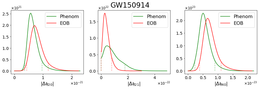
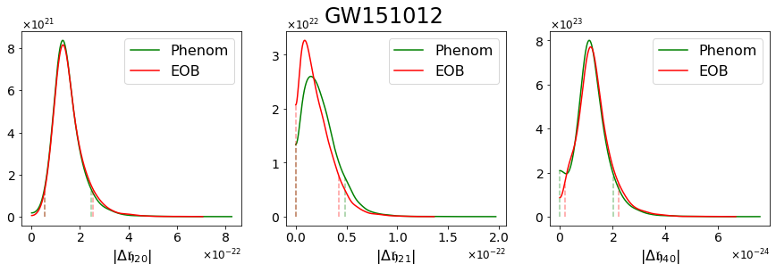
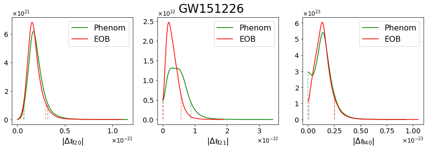
Figure 4: The posterior distributions for the total memory in the $(2,0),\,(2,1)$ and $(4,0)$ modes for the three O1 events. The best fit values of the individual black hole masses for GW150914, GW151012 and GW151226 are respectively $(35.6M_{\odot},30.6M_{\odot})$ $(13.6M_{\odot},15.2M_{\odot})$ and $(7.7M_{\odot},8.9M_{\odot})$. As in the main text, we emphasize again that this not a direct measurement of the memory, but these are instead histograms of the inferred values of the memory relying on waveform models and standard general relativity. The first two events are consistent with non-spinning initial black holes while there is some evidence for moderate spins for GW151226. The red and green vertical dashed lines show the $90\%$ credible intervals (centered around the median) for the corresponding distribution .

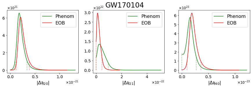
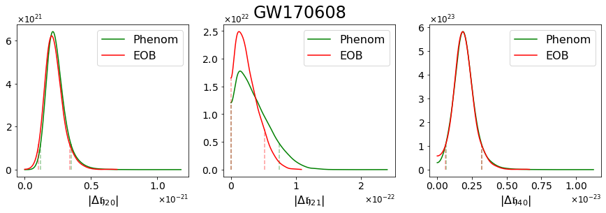
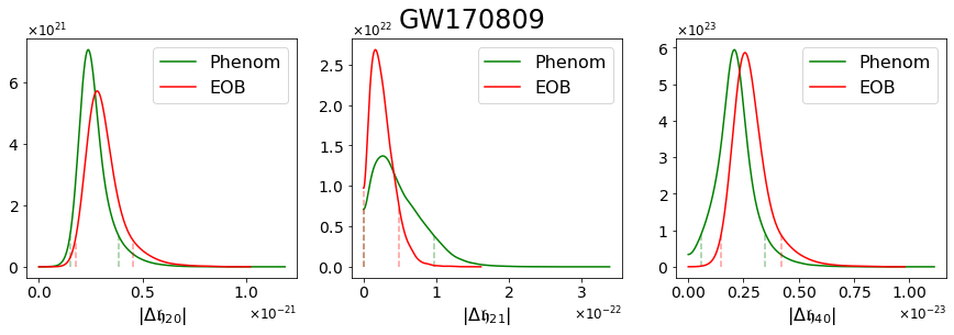
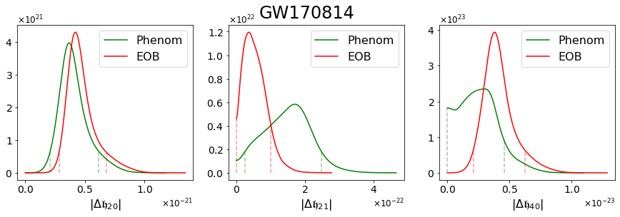
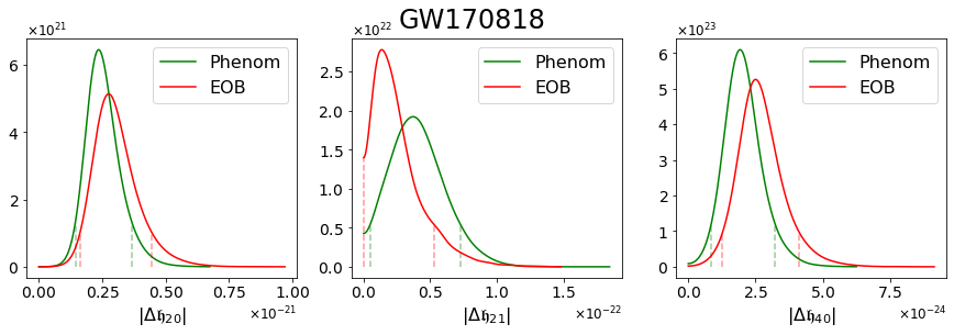
Figure 5: Posterior distributions of the inferred values of the memory for some selected modes. This figure presents results for five of the O2 events, namely GW170104, GW170608, GW170809, GW170814 and GW170818, in each case for both the EOB and Phenom models. Each row of figures corresponds to a particular event, while the first, second and third columns refer to the $(2,0),(2,1)$ and $(4,0)$ modes respectively. These are all systems with moderate mass ratios, with the best fit individual masses being respectively $(20.0M_{\odot},21.4M_{\odot})$, $(11.0M_{\odot},7.6M_{\odot})$, $(35.0M_{\odot},23.8M_{\odot})$, $(30.6M_{\odot},25.2M_{\odot})$ and $(35.4M_{\odot},26.7M_{\odot})$. All of these are consistent with small individual spins. Note that while the posteriors of EOB and Phenom generally agree, there is a large difference for the $(2,1)$ mode for GW170814.

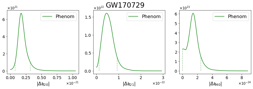
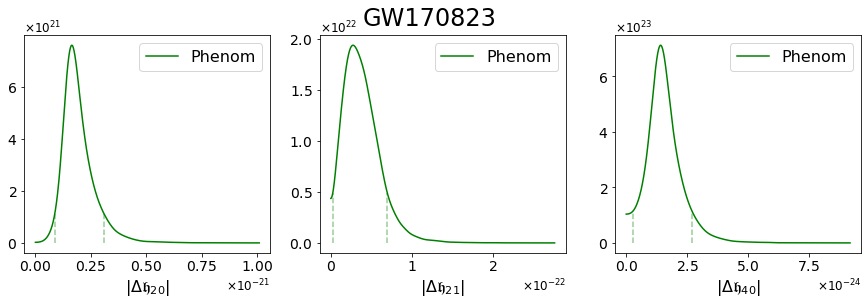
Figure 6: Posterior distributions of the inferred memory for the $(2,0),\,(2,1)$ and $(4,0)$ modes. The respective modes are shown in the first, second and third columns for two of the O2 events GW170729 and GW170823, and for the IMRPhenomPv2 model. The individual masses for these events are respectively $(50.2M_{\odot},34.0M_{\odot})$ and $(39.5M_{\odot},29.0M_{\odot})$. GW170729 has moderately strong evidence of non-negligible spins.

We now implement this procedure for the binary mergers listed in the first Gravitational-Wave Transient Catalog (GWTC-1) Abbott et al. (2019a, b). The catalog lists binary merger events from the first and second observational science runs of the LIGO and Virgo observatories as reported by the LIGO and Virgo Collaborations. The first observational run (01) covers the duration from September 12, 2015 – January 19, 2016 and three binary black hole mergers are reported in GWTC-1 for this period. The second observational run (O2) covers the duration from November 30, 2016 – August 25, 2017. This period has seven binary black hole mergers and a binary neutron star merger as reported in GWTC-1. For each of the events, the LIGO-Virgo Collaboration has released the results of the parameter inference studies with different waveform models, in particular with different variants of the Phenom and EOB models. Several other credible events apart from these have been reported in the literature. We note here in particular the events reported in Venumadhav et al. (2019); Zackay et al. (2019a, b) and in the two Open Gravitational Wave Catalogs (denoted 1-OGC and 2-OGC) Nitz et al. (2019a, b). The analysis of this paper could, of course, be carried out for any of these additional events as well. Since our goal is to compare different waveform models, here we use the results from GWTC-1 only because it reports posterior distributions for both the Phenom and EOB waveform models. Specifically, the posterior distributions use the IMRPhenomPv2 Husa et al. (2016); Khan et al. (2016); Hannam et al. (2014) and SEOBNRv3 Pan et al. (2014b); Taracchini et al. (2014b); Babak et al. (2017). Both of these are complete inspiral-merger-ringdown models including precession. IMRPhenomPv2 uses a single effective spin parameter while SEOBNRv3 uses individual spins for the two black holes. Both of these models use only the $\ell=2$ modes, and are in fact based on applying suitable time dependent rotations to the $\ell=2,m=\pm 2$ modes of an underlying non-precessing model. These rotations can lead, in principle, to all values of $m$, i.e. $-2\leq m\leq 2$ (though the $(2,0)$ mode is generally not well modeled by a single effective spin parameter Schmidt et al. (2012)). Thus, following the rules of addition of angular momentum, it is easy to verify that $|\dot{\mathfrak{h}}|^{2}$ (which leads to the dominant memory contributions) contains modes with $0\leq\ell\leq 4$ and potentially all values of $m$.

We begin with the three O1 events labeled GW150914, GW151012, and GW151226. For each of these events, the distributions of $\Delta\mathfrak{h}_{20}$, $\Delta\mathfrak{h}_{21}$ and $\Delta\mathfrak{h}_{40}$ are shown in Figs. 4. For GW150914 and GW151226 there is moderate disagreement between the Phenom and EOB results, especially for the $(2,1)$ mode. On the other hand, GW151012 shows excellent agreement between the different models. The results for five of the O2 events are shown in Fig. 5. While there are some minor discrepancies for the $(2,0)$ and $(4,0)$ modes, it is evident that again, as for GW150914 and GW151226, the $(2,1)$ mode shows the largest discrepancies for several of the O2 events. All of these five events have moderate mass ratios and are consistent with the initial black holes being non-spinning, and thus the sub-dominant modes due to precession are not likely to have large amplitudes.

It is straightforward to trace back which modes of the waveform $\mathfrak{h}_{\ell m}$ have non-vanishing contributions to a given memory mode $\Delta\mathfrak{h}_{\ell m}$. From Eq. (16), we see that $\mathfrak{h}_{\ell_{1}m_{1}}$ and $\mathfrak{h}_{\ell_{2}m_{2}}$ can contribute to $\Delta\mathfrak{h}_{\ell m}$ only if

$$\begin{pmatrix}\ell_{1}&\ell_{2}&\ell\\ m_{1}&-m_{2}&m\end{pmatrix}\neq 0\,.$$ (19)

From the properties of the 3j-symbols we must then have $m=m_{2}-m_{1}$. The $(2,1)$ memory mode must arise from mode combinations where $m_{1}$ and $m_{2}$ differ by unity. An example of an allowed mode pair would then be products of the $(2,2)$ and $(2,1)$ modes. On the other hand, for the $(2,0)$ or $(4,0)$ mode, we would have $m_{2}=-m_{1}$. This includes for example products of the $(2,2)$ and $(2,-2)$ modes which are better modeled, unlike the $(2,1)$ mode which is generated by the time dependent rotations mentioned above. It is then not surprising that $\Delta\mathfrak{h}_{2,1}$ shows the most discrepancy (However, this argument is not entirely foolproof because the $(2,\pm 1)$ modes contribute to $\Delta\mathfrak{h}_{20}$ as well, though these are presumably generally sub-dominant). This line of reasoning points towards at least a general direction to resolve these differences.

Shown in Fig. 6 are the remaining binary black hole merger events from O2, namely GW170729 and GW170832. For both of these we show only the IMRPhenomPv2 result because of the technical difficulty related to the spin definitions at a reference frequency of $20\,$Hz mentioned earlier. We shall address this elsewhere and here only present the Phenom results.

IV Discussion

Given the required input parameters (see Section I), EOB and Phenom models provide us with a waveform that the detector would receive. Therefore, in any LIGO-Virgo event, the measurement of strain provides us with posterior probability distributions for these parameters. Using the commonly used terminology, we referred to them as measured values. Once we have these posteriors, within any one theory, we can calculate the predicted probability distributions for other observables in that theory. In particular, using general relativity, one can calculate values of the masses, spins and the recoil velocities of the remnants. We referred to these as inferred values. Future measurements with more sensitive detectors will be able to directly measure the memory. Once this happens, comparison of these direct measurements with the inferred values will yield tests of non-linear aspects of general relativity. As shown in previous studies, this could require us to combine $\mathcal{O}(2000)$ events Hübner et al. (2020), or wait for the space based LISA detector Favata (2009b).

Before these direct measurements become reality, apart from improvements in detector sensitivity, it will also be necessary to improve the accuracy of waveform models. We have shown that differences between predictions for inferred observables made by different waveform models can serve as indicators of differences in the underlying physics. In Sec. III.1 we presented an example to illustrate this tool: GW150914. Although the expectation value of the inferred observable $M_{f}$ – the remnant mass – in each model is within 68% confidence level of that in the other, the posterior distribution in Phenom resembles a Gaussian, while that in EOB has a double peak. We found that this difference is most likely because of the difference in the way precession is handled in the two models. For the recoil velocity, both models give inferred values that are orders of magnitude lower than those provided by surrogate fits to numerical relativity. This difference can be traced back directly to the fact that, in the co-precessing frame, neither model includes the modes that contribute to the kick. While this result is not surprising, it provides a proof of principle that the balance laws can be used to test accuracy of candidate waveforms.

More importantly, the infinite tower of constraints pro- vided by the balance laws Eq. (7) can be used to compare and contrast model waveforms. In Sections III.2 and III.3 we used these constraints to infer the posterior distributions for several leading modes in the spherical harmonic decomposition of total gravitational memory. Memory is not an observable of direct astrophysical interest. However, from a fundamental general relativistic point of view, it as a gauge invariant observable associated with the waveform. Therefore, each spherical harmonic component of memory provides us with a new tool to test the accuracy of waveform models. As tools, they are on the same footing as other inferred observables such as the remnant mass and spin. Furthermore, these new tools can reveal discrepancies between waveform models that were not detected by the more commonly used observables that refer only to the properties of the remnant. Finally, note that this analysis is rather different from discussions of gravitational memory in the literature Hübner et al. (2020); Boersma et al. (2020) where the emphasis is on a definitive or direct measurement of gravitational memory from combining several detections. We do not address this interesting issue. By contrast, as we have emphasized, our goal is to regard memory as an inferred observable and use it to probe systematic errors between different waveform models. In particular, our analysis makes a strong use of general relativity because our focus is on testing the accuracy of the candidate waveforms vis-a-vis predictions of exact general relativity.

There are, however, some limitations of this procedure. Once we obtain an event for which the posterior distributions between the models show clear systematic difference, we know that both models cannot be good approximations to exact general relativity in a certain region of the parameter space. As the detector sensitivity increases such pointers could serve as powerful guidelines, calling for further examination of the physics captured by the models. However, it is not straightforward to identify what aspects of the waveforms are causing this difference. Thus, the evaluative role is ‘passive’ in the sense that the pointers by themselves do not provide clear-cut directions to improve the models.

Nevertheless, some preliminary conjectures can be made. The first is, as noted in Sec. III.3, the flux contains products of two modes. Therefore, given pairs $\mathfrak{h}_{\ell_{1}m_{1}}$ and $\mathfrak{h}_{\ell_{2}m_{2}}$, we can identify which mode pair contributes to each $\Delta\mathfrak{h}_{\ell m}$. The second comment is that even if the dominant modes (typically $(2,\pm 2)$) are well modeled, there is still a non-trivial issue, namely, that of correlations between various modes. These are necessary to calculate $|\dot{\mathfrak{h}}|^{2}$ accurately according to Eq. (15) and thus greatly impact the memory. Clearly, larger the precession or more asymmetric the system, larger larger will the impact of the other modes be. It is likely that these configurations will also generally have larger disagreements in the inferred values of the memory in different models. Note that both the EOB and Phenom models do not directly model precession. They both start with an underlying non-precessing model to which the precession effects are applied as suitable time dependent rotations Schmidt et al. (2011); Boyle et al. (2011); Schmidt et al. (2012) (see also Hannam (2014)). It is generally only the underlying non-precessing models which are directly calibrated with numerical relativity waveforms, and the other modes are generated by the time dependent rotations. Thus, it is possible that if precession effects and the higher modes were to be directly calibrated with numerical relativity results, the disagreements with the memory reported here would reduced. It is worth noting that more recent precessing Phenom models for the higher modes labeled IMRPhenomPv3HM London et al. (2018); Khan et al. (2020) already represents an improvement in this direction. In this model, the $(2,1)$ mode for instance is non-vanishing even in the co-precessing frame and is thus not determined entirely by the time dependent rotations. Also noteworthy are the developments on the EOB side regarding higher models, e.g. higher modes for non-precessing systems have been modeled in Cotesta et al. (2018) which could form the basis for including precession effects. Some of the more recent events reported by the LIGO-Virgo collaboration employs these models, and it will be interesting to repeat the analysis of this paper for those events.

Finally, there are also systematic errors involved in our analysis of the ten LIGO-Virgo events. The evaluation of the inferred memory for a waveform model involves calculating the mode decomposition of the integral $\int_{-\infty}^{\infty}|\dot{\mathfrak{h}}|^{2}\,dt$. However, for events considered in this paper, the waveform models used in the publicly available analyses, SEOBNRv3 and IMRPhenomPv2, only include the $(2,2)$ mode in the coprecessing frame. While the physics that is ignored may be unimportant for parameter estimation, it may be very important for the inference of certain modes of the memory. Therefore the inferred memory we calculate may suffer from significant systematic errors. For example the $(2,0)$ mode of the memory is typically  10% larger if higher modes are included in the waveform, and a proper estimation of the recoil velocity requires at least the $(2,1)$ mode. However for the comparison of two models that are attempting to include the same physics, these errors should be identical and a comparison of the posterior distributions is still meaningful. With these limitations in mind, we find that the $(2,0)$ mode and $(2,1)$ mode are most significant sources of memory. A comparison of these modes for the GWTC-1 events we analyzed show that they largely agree across models - indicating that the systematics are mostly under control. However for GW170814 we see that the inferred $(2,1)$ mode of the memory differs significantly between EOB and Phenom models.

There are several interesting avenues to take this work forward. First, there are also angular momentum balance laws Ashtekar et al. (2020) analogous to those for supermomentum, used in this paper. Following a procedure analogous to that of Section III.1, they can be used to construct posterior probability distributions for the spin of the final remnant for any given waveform. For any one waveform, a comparison of this distribution with that provided by numerical relativity provides another measure of the accuracy of that waveform. Similarly, comparisons between the posterior distributions from two different waveform models can serve as additional and distinct tests of the differences between the physical underpinning. Returning to gravitational memory, an obvious avenue is to extend our analysis to the more recently reported merger events from the third LIGO-Virgo observational run which includes events with higher masses and more asymmetric mass ratios Abbott et al. (2020a, b). These events could allow for more stringent comparisons between the most up-to-date waveform models. As mentioned above, apart from looking at particular events, it would be useful to compare waveform models using the memory across large parameter space regions. Injections of gravitational waves spanning the parameter space can be performed to learn where the systematic differences are prominent. Alternatively one could avoid parameter estimation results altogether and directly compare deviations in the inferred memory across parameter space. Additionally once we identify the regions of parameter space where these differences arise, such as what we see for GW170814, one can take sample points from the region and directly compare the waveforms and all the components that go into the inference. This should allow one to pinpoint more accurately the source of the deviations between the models, giving more direct input to improve future modeling.

Finally, in this paper, we focused just on total memory that involves integrals from $t=-\infty$ to $t=\infty$ (see Eq. (9)). As pointed out in Ashtekar et al. (2019), there are also finite time versions of balance laws that enable one to calculate the memory as a function of time, not just the difference between very late and very early times. This involves an accurate calculation of, say, the $(2,0)$ and $(4,0)$ modes and a better understanding of $\Psi_{2}$ Mitman et al. (2020). These calculations will lead to much more detailed accuracy tests on waveforms. Longer term, over the next decade, as more sensitive detectors are commissioned and more accurate waveform models are developed and the memory is observed directly, the most important payoff will be to compare the inferred values of the memory modes with the observed values, thereby providing a test of non-linear general relativity.