Finding Acceptable Parameter Regions of Stochastic Hill functions for Multisite Phosphorylation Mechanism

Abstract

Multisite phosphorylation plays an important role in regulating switchlike protein activity and has been used widely in mathematical models. With the development of new experimental techniques and more molecular data, molecular phosphorylation processes emerge in many systems with increasing complexity and sizes. These developments call for simple yet valid stochastic models to describe various multisite phosphorylation processes, especially in large and complex biochemical networks. To reduce model complexity, this work aims to simplify the multisite phosphorylation mechanism by a stochastic Hill function model. Further, this work optimizes regions of parameter space to match simulation results from the stochastic Hill function with the distributive multisite phosphorylation process. While traditional parameter optimization methods have been focusing on finding the best parameter vector, in most circumstances modelers would like to find a set of parameter vectors that generate similar system dynamics and results. This paper proposes a general $\alpha$-$\beta$-$\gamma$ rule to return an acceptable parameter region of the stochastic Hill function based on a quasi-Newton stochastic optimization (QNSTOP) algorithm. Different objective functions are investigated characterizing different features of the simulation-based empirical data, among which the approximate maximum log-likelihood method is recommended for general applications. Numerical results demonstrate that with an appropriate parameter vector value, the stochastic Hill function model depicts the multisite phosphorylation process well except the initial (transient) period.

1 Introduction

Protein phosphorylation is a fundamental molecular mechanism that regulates protein function through the addition of a phosphate group. Many proteins have multiple phosphorylation sites and the phosphorylation process often targets multiple distinct sites, referred to as multisite phosphorylation. Multisite phosphorylation facilitates the complexity and scope of protein activity and is ubiquitous in biological processes such as cell cycle regulation [2]. Over the years, researchers have revealed that multisite phosphorylation forms the basis of switchlike response [14] and can exhibit bistability and periodic oscillations [21, 34, 5].

Based on the enzyme (kinase) processivity, there are two categories of multisite phosphorylation mechanisms [36]. The processive mechanism occurs when the enzyme phosphorylates all sites without dissociation from the substrate, while in the distributive mechanism, the enzyme dissociates from its substrate after one site becomes phosphorylated. This paper considers the multisite phosphorylation process with an ordered distributive mechanism, shown by

$${\rm B}_{0}\xrightleftharpoons[b_{1}]{f_{1}[{\rm A}]}{\rm B}_{1}\xrightleftharpoons[b_{2}]{f_{2}[{\rm A}]}{\rm B}_{2}\ldots\xrightleftharpoons[b_{n-1}]{f_{n-1}[{\rm A}]}{\rm B}_{n-1}\xrightleftharpoons[b_{n}]{f_{n}[{\rm A}]}{\rm B}_{n}.$$ (1)

B is a protein (substrate) with $n$ phosphorylation sites. A is the enzyme (kinase) that can bind to substrate B. ${\rm B}_{0}$ represents the unphosphorylated form (unbound to any phosphoryl group), and ${\rm B}_{n}$ is the fully phosphorylated form. ${\rm B}_{n}$ is formed in sequential steps, with intermediate stages increasing by one site phosphorylated until all $n$ sites are phosphorylated. Assume that there are enough phosphate groups for the phosphorylation process in system (1) and all binding sites are the same (no preference over the selection of binding sites). Enzyme A controls the phosphorylation of ${\rm B}_{i}$ with the phosphorylation activity $f_{i}[\rm A]$, where $f_{i}$ is the phosphorylation rate and $[\rm A]$ denotes the quantity (population or concentration) of the enzyme A. In the stochastic regime, [A] represents the enzyme population. $b_{i}$ $(i=1$, $2$, $\ldots$, $n)$ denotes the dephosphorylation activity of ${\rm B}_{i}$, where $b_{i}={k_{i}}[{\rm phosphotase}]$. Assuming that the phosphotase level is constant in the enzyme-substrate system (1), one can simply use $b_{i}$ to represent the product of dephosphorylation rate $k_{i}$ and phosphotase level.

The kinetic behavior of multisite phosphorylation can be mathematically modeled by a set of differential equations based on a series of elementary reactions describing the enzyme-substrate binding and catalysis process. Thus, the concentrations of all possible phosphorylated forms ${\rm[B}_{i}]$ is controlled by

$$\left\{\begin{aligned} &\frac{d[{\rm B}_{0}]}{dt}=b_{1}[{\rm B}_{1}]-f_{1}[{\rm A}][{\rm B}_{0}],\\ &\frac{d[{\rm B}_{i}]}{dt}=f_{i}[{\rm A}][{\rm B}_{i-1}]+b_{i+1}[{\rm B}_{i+1}]-(f_{i+1}[{\rm A}]+b_{i})[{\rm B}_{i}],\text{ for }0<i<n,\\ &\frac{d[{\rm B}_{n}]}{dt}=f_{n}[{\rm A}][{\rm B}_{n-1}]-b_{n}[{\rm B}_{n}].\\ \end{aligned}\right.$$ (2)

The above differential equations are a traditional deterministic method for modeling and simulating the multisite phosphorylation. While in the stochastic regime, the enzyme-substrate system is governed by a list of reaction propensities, which describe the probabilities of reaction events. Below are the reactions and corresponding propensities for the multisite phosphorylation system (1), where $0<i\leq n$.

Table 1: Chemical reaction and propensity calculation

Reaction	Propensity
${\rm B}_{i-1}\xrightarrow{f_{i}[{\rm A}]}{\rm B}_{i}$	$a=f_{i}[{\rm A}][{\rm B}_{i-1}]$
${\rm B}_{i}\xrightarrow{~{}~{}b_{i}~{}~{}}{\rm B}_{i-1}$	$a=b_{i}[{\rm B}_{i}]$

In the above chemical reactions, if we treat [A] as a constant (parameter), the system (1) becomes a linear reaction network. There are many studies on the stochastic kinetics and efficient modeling and simulation of such chemical reaction networks [6, 26, 12, 16, 23]. For example, Gadgila et al. [16] formulated the governing master equations of first order reactions and results showed that the distribution of all the system components in an open system follows Poisson distribution at steady state. Lente [23] developed a stochastic mapping for first order reaction networks to help evaluate the appropriate method between stochastic and deterministic approaches. Our recent work [26] also presented a numerical analysis for the accuracy of the hybrid ODE/SSA method on linearly reacting systems.

However, for complex biochemical networks involving multisite protein phosphorylation, the above kinetic system in both deterministic and stochastic regimes increases the model size and complexity especially when $n$ is large (a protein with $n$ phosphorylation sites has potentially $n$ to $2^{n}$ distinct phosphorylation forms.) On the other hand, when trying to formulate a realistic multisite phosphorylation system, little is known beyond specific enzyme-substrate systems. Usually, most reaction rates are tuned to match with empirical observations and assumptions are made with limited biological justification. Considering the complexity and lack of knowledge, this paper proposes to model the multisite phosphorylation with a Hill function system and study the dynamic behavior of the fully phosphorylated form ${\rm B}_{n}$.

The Hill equation is widely used in biochemical networks to model fast signal response and complex binding processes. It was first introduced to model the observed curves of ligand binding to the receptor [20]. The equation is a nonlinear function of the ligand concentration, and the Hill exponent defines the degree of cooperativity of ligand binding. Other complex models have been proposed to describe different cooperativity of ligand binding [1, 30, 22, 28]. The sigmoidal curves generated from the Hill function system is similar to the switchlike protein activity. Furthermore, the Hill equation requires little prior knowledge of the binding mechanism and is much simpler than the kinetic model (2). Therefore, this work investigates the simple Hill function system for the ordered distributive enzyme-substrate system (1):

$${\rm B}_{0}\xrightleftharpoons[\displaystyle k_{d}]{\displaystyle k_{a}\frac{[{\rm A}]^{\sigma}}{k_{m}^{\sigma}+[{\rm A}]^{\sigma}}}{\rm B}_{n},$$ (3)

where $k_{a}$ and $k_{d}$ are the forward and reverse reaction constant, respectively, $k_{m}$ is the dissociation constant, and $\sigma$ is the Hill exponent, a real number with range $\sigma\leq n$.

Since the Hill equation has been thoroughly studied and extensively used in traditional deterministic models (differential equations), the unexplored discrete stochastic representation gets more attention from researchers with the presence of low population levels and molecular noise. Previous studies have discovered that the sigmoidal behavior of the Hill function dynamics may reduce to a linear function in the stochastic regime, especially under the reaction-diffusion master equation framework [11]. This paper models the Hill function system in the stochastic regime and restricts attention to a homogeneous domain. Using the stochastic simulation algorithm (SSA) [18], the above Hill function system (3) is then governed by the forward and reverse reactions with propensities:

$$a_{f}=k_{a}\frac{[{\rm A}]^{\sigma}}{k_{m}^{\sigma}+[{\rm A}]^{\sigma}}[{\rm B}_{0}];\quad a_{r}=k_{d}[{\rm B}_{n}].$$ (4)

Biologists are able to quantify species population at molecular levels with improved experimental techniques [32], which provides good resources (observed empirical data) for validating stochastic models and optimizing “stochastic parameters”. Assuming the ordered distributive mechanism (1) is the ground truth for the multisite phosphorylation process, the trajectories of $[{\rm B}_{n}]$ generated from the stochastic enzyme-substrate system (1) can be considered empirical data, while the trajectories of $[{\rm B}_{n}]$ generated from the stochastic Hill function system (3) are considered as simulated data. This paper, instead of validating the stochastic results against the deterministic results, will focus on optimizing the stochastic Hill function model for the multisite phosphorylation process, meaning optimizing the parameter vector $\theta=[k_{a}$, $k_{d}$, $\sigma$, $k_{m}]$ defining the stochastic Hill function model.

The challenges of solving the inverse problem of parameter estimation for modeling biological systems are manifold. One major challenge is large biological networks with many unknown parameters that are hard or impossible to measure in experiments. The nonlinear nature of the models involves a nonconvex problem with multiple locally optimum points, and local optimization methods may be trapped at local optimum points. Global optimization methods can be very expensive in high dimensions, and global optimality is often not guaranteed [4]. Moreover, most of the efforts in solving such problems thus far have been focused on deterministic models, particularly estimating the parameters of models formulated by nonlinear differential equations [27]. Parameter estimation in stochastic models is even more challenging as the amount of empirical data must be large enough to obtain statistically valid parameter estimates. Two well-known approaches for stochastic optimization problems are stochastic approximation (SA) and response surface methodology (RSM). The class of quasi-Newton methods for stochastic optimization extends state-of-the-art numerical optimization methods (e.g., secant updates, trust regions) [8], can also be used for deterministic global optimization with minor variations [13, 3], and has been successfully applied to various stochastic optimization problems, such as cell cycle models [9], bistable models [10], and biomechanics problems [31]. Other approaches such as Bayesian inference [25, 33], Kalman filter, and its variants [24] have been applied to solve this problem as well. Recently, machine learning techniques have been tailored by sparsity-promoting methods to identify not only the parameters but also the structure of both ordinary differential equations [7] and partial differential equations [35].

Most parameter optimization methods only return a single best parameter vector, regardless of the fact that there are many parameter vectors that could generate similar system dynamics and characteristics. Take the bistable switch in the cell cycle as an example [17]. Bistable phenomena occur when model parameters are inside the bistability region. The entire bistability region or at least most parameter values sampled in the region may be considered acceptable if the goal is to simply model the bistable switch process, rather than to minimize the objective function. This work focuses on finding an “acceptable" parameter region, where parameter vectors in the acceptable region are good alternatives to the best parameter vector minimizing the objective function. In other words, the system parameters are given by a region in parameter space rather than a single point.

This work studies acceptable parameter regions of the stochastic Hill function (3) for the multisite phosphorylation system (1). Section 2 introduces the chemical master equation for deriving the transition probability matrix and the quasi-Newton algorithm used for stochastic optimization. In Section 3, three objective functions measuring different features of the simulation-based empirical data are investigated. Section 4 then presents the proposed $\alpha$-$\beta$-$\gamma$ rule for defining the acceptable parameter regions found by the quasi-Newton stochastic optimization (QNSTOP) algorithm. Numerical results and detailed analyses are given in Section 5.

2 Background

This section first reviews the chemical master equation and the analytical solution of a general biochemical system. Then, the essential steps of the quasi-Newton stochastic optimization algorithm (QNSTOP) are summarized.

2.1 Chemical Master Equation

Consider a well-mixed system of $N$ distinct species and $M$ reaction channels with $\hat{N}$ possible states. The chemical master equation [19] that describes the probabilistic time evolution of the system dynamics is

$$\frac{d}{dt}{{P}}({X};t)={P}({X};t){C},$$ (5)

where ${X}=[{x_{1}},{x_{2}},\ldots,{x_{\hat{N}}}]$ is all possible state vectors $x_{i}$ at any time $t$, $P({X};t)$ represents the probabilities of those state vectors at time $t$, and ${C}$ is the state reaction matrix [29], given by

$${C}_{ij}=\left\{\begin{array}[]{c c}-\sum_{\mu=1}^{M}a_{\mu}({x}_{j}),&\text{for }i=j,\\ a_{\mu}({x}_{i}),&\text{for }i\text{ such that }{x}_{j}={x}_{i}+v_{\mu},\\ 0,&\text{otherwise},\end{array}\right.$$ (6)

where $v_{\mu}$ is the stoichiometric transition vector for reaction channel $\mu$.

From equation (5), the solution is

$${P}=P_{0}e^{Ct},$$ (7)

where $P_{0}$ is the initial probability of all the possible states, and the transition probability matrix can be calculated by

$${\mathcal{T}}=e^{{C}\tau},$$ (8)

where $\tau$ is the period of time the system has evolved from a previous time [29].

2.2 Quasi-Newton Stochastic Optimization Algorithm

QNSTOP is a class of quasi-Newton methods developed for stochastic optimization [8], where the objective function $f(X)$ is a random variable, and $X$ is contained in a box $L\leq X\leq U$. The essential steps of QNSTOP are summarized here. Further details on the algorithm and implementation can be found in Ref. [3].

• In each iteration $k$, construct a quadratic model

  $$\widehat{m}_{k}(X-X_{k})={\hat{f}}_{k}+{\hat{g}}_{k}^{T}\left(X-X_{k}\right)+\frac{1}{2}\left(X-X_{k}\right)^{T}{\hat{H}}_{k}\left(X-X_{k}\right)$$

  centered at $X_{k}$, where ${\hat{g}}_{k}$ is the gradient vector and ${\hat{H}}_{k}$ is the Hessian matrix. Note that ${\hat{f}}_{k}$ is generally not ${f}{(X_{k})}$, which is stochastic.

• QNSTOP uses an ellipsoidal region centered at the current iterate $X_{k}\in\mathop{\rm I\!R}\nolimits^{n}$ with radius $\tau_{k}$,

  $$E_{k}(\tau_{k})=\left\{X\in\mathop{\rm I\!R}\nolimits^{n}:\left(X-X_{k}\right)^{T}W_{k}\left(X-X_{k}\right)\leq\tau_{k}^{2}\right\},$$

  where $W_{k}$ is a symmetric, positive definite scaling matrix, satisfying $W_{k}\in W_{\gamma}$,

  $${W_{\gamma}=\bigl{\{}W\in\mathop{\rm I\!R}\nolimits^{n\times n}:W=W^{T},\det(W)=1,\gamma^{-1}I_{n}\preceq W\preceq\gamma I_{n}\bigr{\}}}$$

  for some $\gamma\geq 1$, where $I_{n}$ is the $n\times n$ identity matrix, and $A\preceq B$ means $B-A$ is positive semidefinite. The elements of the set ${\bf{\rm W}}_{\gamma}$ are valid scaling matrices that control the shape of the ellipsoidal design regions with eccentricity constrained by $\gamma$.

• Then QNSTOP estimates the gradient based on a set of $N$ uniformly sampled design sites $\{X_{k1}$, $\ldots$, $X_{kN}\}\subset E_{k}(\tau_{k})\cap\Theta$ ($\Theta=[L,U]$, which is the feasible set of parameters defined initially.) For the Hessian matrix, QNSTOP uses either a variation of the SR1 (symmetric, rank one) quasi-Newton update (stochastic $f$) or the unconstrained BFGS quasi-Newton update (global optimization of deterministic $f$).

• For the next iteration, by utilizing an ellipsoidal trust region concentric with the design region for controlling step length, $X_{k+1}$ is updated as

  $$X_{k+1}=\left(X_{k}-\left[{\hat{H}}_{k}+\mu_{k}W_{k}\right]^{-1}\hat{g}_{k}\right)_{\Theta},$$

  where $\mu_{k}$ is the Lagrange multiplier of a trust region subproblem, and $\left(\cdot\right)_{\Theta}$ denotes projection onto the feasible set $\Theta=[L,U]$.

• Finally, the experimental design region $E_{k}(\tau_{k})$ is updated to approximate a confidence set by updating the scaling matrix $W_{k}$. The updated scaling matrix is given by

  $$W_{k+1}=\left(\hat{H}_{k}+\mu_{k}W_{k}\right)^{T}V_{k}^{-1}\left(\hat{H}_{k}+\mu_{k}W_{k}\right),$$

  where $V_{k}$ is the covariance matrix of $\nabla\widehat{m}_{k}(X_{k+1}-X_{k})$. For numerical stability, $W_{k+1}$ is constrained (by modifying its eigenvalues) to satisfy the constraints $\gamma^{-1}I_{n}\preceq W_{k+1}\preceq\gamma I_{n}$ and $\det(W_{k+1})=1$, so $W_{\gamma}\ni W_{k+1}$.

3 Objective Functions

This section presents three different objective functions characterizing different aspects of the population trajectory of ${\rm B}_{n}$. In particular, we propose a general simulation-based objective function that can be applied to large biochemical networks.

3.1 Minimum distance area

In the enzyme-substrate system (1), suppose $D=[\hat{x}_{1}$, $\hat{x}_{2}$, $\ldots$, $\hat{x}_{m}]$ is a sequence of the molecular population of ${\rm B}_{n}$ collected from stochastic simulation results after every time $\tau$ (denoted as $[t_{1}$, $t_{2}$, $\ldots$, $t_{m}]$), where $m$ is the data size. This subsection will consider the population difference of ${\rm B}_{n}$ between the empirical data (from multisite phosphorylation) and simulation results (from stochastic Hill function) over time, called the distance area. Given the empirical data and the simulated data as two vectors, the $p$-norm is one traditional way to measure the vectors’ difference. The problem is stochastic and the time series data can be quite noisy, and outliers have more influence for $p>1$, hence the 1-norm is used to measure the distance. Define the distance area as the objective function,

$$f_{d}(\theta)=\int|p(t)-q(t)|dt\approx\sum_{i=1}^{m}|\hat{x}_{i}-\hat{y}_{i}|\tau,$$ (9)

where $\theta$ is the vector of model parameter values, $p(t)$ and $q(t)$ are the trajectory functions of empirical and simulated populations in continuous domains. For discrete time series data, $\hat{x}_{i}$ and $\hat{y}_{i}$ represent the population of ${\rm B}_{n}$ from empirical and simulated data, respectively. The stochastic optimization problem to be solved is

$$\min_{\theta\in\Theta}f_{d}(\theta),$$ (10)

where $\Theta\subset{\rm I\!R}^{n}$ defines the feasible set (allowable values for the model parameter vector $\theta$).

3.2 Maximum log-Likelihood

The minimum distance area, similar to other traditional optimization methods, builds objective functions based on ‘mean’ measurements from stochastic simulations, hence cannot reflect the intrinsic noise in stochastic models. To capture the stochastic fluctuations, measure the transition probability that a system jumps from one state to the next state after a certain time step. The likelihood function of time series data can then be factorized into the product of transition probabilities. For convenience, the logarithm of the likelihood, which changes a product to a sum, is used. The logarithm of the likelihood of the observed data $D$ is

$$\log\mathcal{L}({\theta}|{D})=\log\bigg{(}\prod_{i=2}^{m}{{\mathcal{T}}}_{x_{i-1},x_{i}}\bigg{)}=\sum_{i=2}^{m}\log{{\mathcal{T}}}_{x_{i-1},x_{i}}$$ (11)

where $\theta\in{\rm I\!R^{n}}$ is the vector of model parameter values and ${\mathcal{T}}$ is the transition probability matrix. Specifically, ${\mathcal{T}}_{x_{i-1},x_{i}}$ is the transition probability that the system changes from state $x_{i-1}$ to state $x_{i}$. Note that we take the logarithm of the likelihood because the transition probability matrix is usually very close to zero. The log-Likelihood function expresses the probabilities of the observed empirical data for different values of parameter vector $\theta$. A larger value of log-likelihood indicates a better fit to the empirical data.

Using the maximum log-likelihood, the objective function is

$$f_{l}(\theta)=-\log\mathcal{L}({\theta}|{D}),$$ (12)

and the stochastic optimization problem to be solved is

$$\min_{\theta\in\Theta}f_{l}(\theta),$$ (13)

where $\Theta$ is a set in ${\rm I\!R^{n}}$ defining the feasible set (allowable values for the model parameter vector $\theta$).

When a system has a finite number of states, then we can calculate $\mathcal{T}$ directly from Eq. (8). When a system is small and has an infinite number of states, the finite state projection (FSP) method [29] projects the infinite state vector ${X}$ to a finite state vector, approximating the CME solution with an error $\epsilon$. Accordingly, ${C}$ and ${\mathcal{T}}$ are approximated by ${\hat{C}}$ and ${\hat{\mathcal{T}}}$, respectively. Fox et al. [15] proved that the FSP-derived likelihood converges monotonically to the exact likelihood value.

3.3 Approximate maximum log-likelihood

In the above maximum log-likelihood method, the approximation of the transition matrix ${\mathcal{T}}$ is only tractable for small systems. It is difficult or nearly impossible to solve the CME for large systems. To overcome this limitation, this subsection proposes an approximate maximum log-likelihood method, a general use objective function that is applicable to large complex biochemical networks.

The transition probability of system state going from $x_{i-1}$ to $x_{i}$ is

$${\mathcal{T}}_{x_{i-1},x_{i}}={\rm Pr}(x_{i}|x_{i-1}).$$ (14)

Thus, the logarithm of the likelihood of the empirical data $D$ is

$$\log\mathcal{L}({\theta}|{D})=\log\bigg{(}\prod_{i=2}^{m}{{\rm Pr}(x_{i}|x_{i-1})}\bigg{)}=\sum_{i=2}^{m}\log{\rm Pr}(x_{i}|x_{i-1}),$$ (15)

where ${\rm Pr}(x_{i}|x_{i-1})$ can be approximated using simulation data (An example will be shown later in (19)). The objective function of approximate maximum log-likelihood is

$$f_{p}(\theta)=-\log\mathcal{L}({\theta}|{D}).$$ (16)

The stochastic optimization problem to be solved is

$$\min_{\theta\in\Theta}f_{p}(\theta),$$ (17)

where $\Theta$ is a set in ${\rm I\!R^{n}}$ defining the feasible set.

Algorithm 1 summarizes the essential steps of the approximate maximum log-likelihood method. In Line 6, by simulating the system $q$ times from time $t_{i-1}$ to $t_{i}$ with initial system state $[{\rm B}_{n}]=x_{i-1}$, we get a list of simulation results for $[{\rm B}_{n}]$ at time $t_{i}$, represented as $S_{i}=[s_{1}$, $s_{2}$, $\ldots$, $s_{q}]$. ${\rm Pr}(x_{i}|x_{i-1})$ can be approximated from the distribution of $S_{i}$. For example, assuming $x_{i}$ (sampled in $S_{i}$) follows a normal distribution

$$x_{i}\sim N(\mu,\sigma^{2}),$$ (18)

where $\mu$ and $\sigma^{2}$ are the mean and variance of $x_{i}$, we can approximate the probability as

$${\rm Pr}(x_{i}|x_{i-1})\approx{\rm Pr}(x_{i}-0.5<\mu+\sigma z_{i}<x_{i}+0.5),\quad z_{i}=\frac{x_{i}-\mu}{\sigma}\sim N(0,1).$$ (19)

Note that the empirical data could be multiple species’ population trajectories, then $x_{i}$ in ${\rm Pr}(x_{i}|x_{i-1})$ becomes a vector referring to multiple species’ population. In Line 4, if the simulation results do not include $[{\rm B}_{n}]=\hat{x}_{i}$, then choose one that is the closest to $\hat{x}_{i}$.

Algorithm 1 Approximate maximum log-likelihood

1:Empirical data $D=[\hat{x}_{1}$, $\hat{x}_{2}$, $\ldots$, $\hat{x}_{m}]$ represents the population trajectory of species $[{\rm B}_{n}]$

2:$-\sum_{i=2}^{m}\log{\rm Pr}(\hat{x}_{i}|\hat{x}_{i-1})$

3:Initialization $i=2$, system state $\hat{x}_{1}$.

4:while $i\leq m$ do

5:   if $i=2$ then go to line 6

6:   else initialize the system with the simulation result where $[{\rm B}_{n}]=\hat{x}_{i-1}$ at time $t_{i-1}$

7:   end if

8:   Simulate the system $q$ times from time $t_{i-1}$ to $t_{i}$ generating a list of simulation results for ${\rm B}_{n}$ at time $t_{i}$, denoted as $S_{i}=[s_{1}$, $s_{2}$, $\ldots$, $s_{q}]$.

9:   Construct ${\rm Pr}(\hat{x}_{i}|\hat{x}_{i-1})$ based on the distribution of $S_{i}$

10:   $i=i+1$

11:end while

4 Acceptable Parameter Region

As mentioned before, for most systems, especially those with multidimensional parameters, there are possibly many combinations of parameter values producing similar system dynamics and behaviours. This section introduces the $\alpha$-$\beta$-$\gamma$ rule to find the acceptable parameter regions of the stochastic Hill function. Parameter values sampled in an acceptable region should have similar system results compared to the best parameter values. In particular, we applied the $\alpha$-$\beta$-$\gamma$ rule to QNSTOP, which has been used to find the best parameter values of several stochastic problems.

4.1 $\alpha$-$\beta$-$\gamma$ Rule

Based on the fact that QNSTOP creates an ellipsoidal design region at each iteration, we can utilize this ellipsoid to define the acceptable parameter region. For an ellipsoid $E$, define the objective function values as $f(E)=\{f(x)\mid x\in E\}$. To accept a parameter region, intuitively, most parameters sampled from the region should have relatively small objective values, and close to the minimum objective function value of the ellipsoidal region, written as $\min f(E)$. Based on scrutinizing all possible distributions of $f(E)$, define a stable ellipsoidal region $E$ as follows:

Definition 4.1.

Assume $f(\theta)\geq 1$ always. $E$ is a min-stable region if

$${\rm Pr}\big{[}f(\theta)\leq(1+\alpha)\min f(E)\big{]}\geq\beta,\quad\theta\in E,\ \alpha\in(0,\infty),\ \beta\in(0,1].$$

In the above definition, $\alpha$ measures how close the objective function values are to the minimum value $\min f(E)$, $\beta$ controls the percentage of parameter values that generate close minimum objective function values. $\alpha$ and $\beta$ can be assigned with different values depending on the problem. For any parameter region $E$, if $\alpha$ is fixed, define the percentage of points with objective function values no larger than $(1+\alpha)\min f(E)$ as the region stability, which is the value of ${\rm Pr}\big{[}f(\theta)\leq(1+\alpha)\min f(E)\big{]}$.

As QNSTOP designs a specific ellipsoidal region at each iteration, the minimum objective function values found may vary dramatically between iterations. We don’t want to accept the ellipsoidal region $E_{1}$ of the first iteration even if $E_{1}$ is min-stable, because $\min f(E_{1})$ is usually much larger than the minimum objective value $f_{min}$ found over all iterations and all starting points (if QNSTOP is run with multiple starting points). Thus, to ensure that the parameter region is globally min-stable, we need to choose those min-stable regions whose local minimum objective function values are close to the lowest minimum found so far. The acceptable parameter region is defined as a union of min-stable ellipsoids with local minimum objective function values close to $f_{min}$:

Definition 4.2.

An acceptable region is $\displaystyle R=\bigcup_{k\in{\mathcal{B}}}E_{k}$ where

$${\mathcal{B}}=\{k\ |\ E_{k}\ \text{is min-stable and}\ \min f(E_{k})\leq(1+\gamma)f_{min}\big{\}},\quad\gamma\in[0,\infty).$$

In the above definition, $k$ is the iteration number, $\gamma$ controls how close $\min f(E_{k})$ is to the lowest minimum found over all iterations, and $\gamma$ may vary according to the problem. Choosing values for $\alpha$, $\beta$, $\gamma$ is referred to as the $\alpha\hbox{-}\beta\hbox{-}\gamma$ rule. Note that if optimization algorithms use multiple starting points, then $k$ indexes iterations over all starting points, and $f_{min}$ is the minimum found over all starting points.

4.2 Analysis

Values for $\alpha$, $\beta$, and $\gamma$ are derived from analyzing the objective function values in parameter regions. Fig. 1 shows the distributions of the three objective function values over several iterations. For iteration 10, $f(X)$ of maximum log-likelihood method is almost a uniform distribution, with values spread out over the domain. As the iteration continues, more objective function values are getting closer to $f_{min}$, the minimum value found so far. The distribution of $f(X)$ gradually forms a peak around $f_{min}$. While these features hold for all three methods, the maximum log-likelihood has the highest percentage of the small objective values. Based on the distributions, the values of $\alpha$ for the three methods are chosen as 0.5 (minimum distance area), 0.2 (maximum log-likelihood), 0.3 (approximate maximum log-likelihood), respectively. Fig. 2 illustrates how the ellipsoidal regions of parameters $k_{a}$, $k_{d}$ shrink over iterations.

(a) Minimum distance area

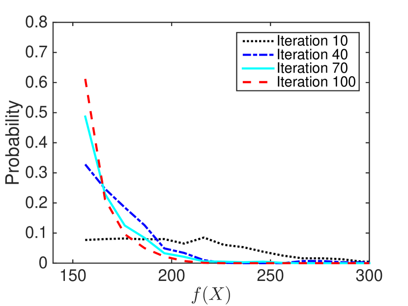
(b) Maximum log-likelihood

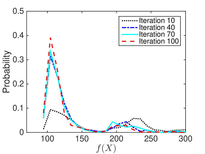
(c) Approximate maximum log-likelihood

Figure 1: Distributions of objective function values from three methods (minimum distance area, maximum log-likelihood, and approximate maximum log-likelihood) based on 1000 sampled points inside the ellipsoidal regions for iterations 10, 40, 70, and 100.

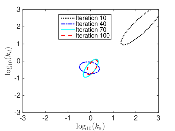
Figure 2: QNSTOP ellipsoids at iterations 10, 40, 70, and 100 from the maximum log-likelihood method.

Figure 3 shows that for all three methods, the average region stability (defined before) over 100 starting points increases with iteration number. The maximum log-likelihood has the highest region stability compared to the other two objective functions. For the maximum log-likelihood method, $\alpha=\gamma=0.2$ and $\beta=0.8$ based on the region stability. In this way, at least 80% of the sampled points from the acceptable region have objective function values within 20% relative error of the minimum value, called the 80%-20% rule. For the other two methods, $\alpha=\gamma=0.3$, $\beta=0.7$ for approximate maximum log-likelihood, and $\alpha=\beta=\gamma=0.5$ for minimum distance area.

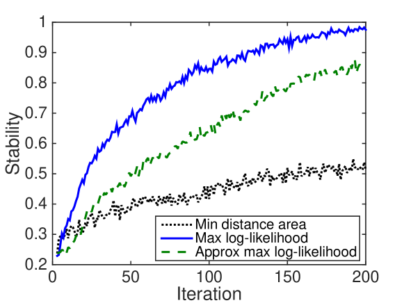
Figure 3: Average region stability from iteration 1 to 200 based on 100 starting points from minimum distance area ($\alpha=0.5$), maximum log-likelihood ($\alpha=0.2$), and approximate maximum log-likelihood ($\alpha=0.3$).

5 Results

This section first discusses the experimental setup including the empirical data and input parameters. Then the optimization results are divided into two parts. The first part demonstrates the result of optimizing two parameters, $k_{a}$ and $k_{d}$; the second part compares the three objective functions and studies the full parameter vector $\theta$.

5.1 Experimental setup

Empirical data. This work assumes the ordered distributive multisite phosphorylation system (1) as the ground truth. In particular, consider the system size $n=4$, the population level of enzyme $[{\rm A}]=1000$, and the reaction constants $f_{i}=0.0025$, $b_{i}=1$ for $i=1$, $2$, $3$, $4$. The initial condition is $[{\rm B}_{0}]=100$, $[{\rm B}_{i}]=0$ for $0<i\leq n$. Use the stochastic simulation algorithm to simulate the system and sample one population trajectory of ${\rm B}_{n}$ with a time step $\tau$ $(t_{1}=\tau$, $t_{2}=2\tau$, $\ldots$, $t_{m}=m\tau)$ as a single set $D$ of empirical data. Since both systems (1) and (3) stabilize at a steady state after a certain time (transition period), if the empirical data $D$ contains more steady state information than transition period, then the system parameters will be optimized in a way that minimizes the difference of steady states but overlooks the transition dynamics before the system stabilizes, and vice versa. Therefore, the empirical data points are sampled equally covering both the transition and stable periods.

The stochastic Hill function system (3) has an initial condition $[{\rm B}_{0}]=100$ and $[{\rm B}_{n}]=0$, thus there are at most 101 system states. Table 2 lists the bounds for each parameter in the system.

Table 2: Parameter boundary in the stochastic Hill function system.

Parameter	$k_{a}$	$k_{d}$	$k_{m}$	$\sigma$
$[L,U]$	$[0.001,1000]$	$[0.001,1000]$	$[0.001,10^{6}]$	$[0.001,10]$
$\log_{10}([L,U])$	$[-3,3]$	$[-3,3]$	$[-3,6]$	$[-3,1]$

Note that parameters $k_{a}$ and $k_{d}$ (rate constants of association and dissociation) control the system’s time scale. For fixed parameters $k_{m}$ and $\sigma$, while parameter region $[0.001,1]$ for $k_{a}$ and $k_{d}$ occupies 0.0001% of the entire search box, the system time scale varies by three orders of magnitude. In Fig. 4, the final population of ${\rm B}_{n}$ initially grows linearly (in logarithm) with $k_{a}/k_{d}$ and then levels off around 100. When $k_{a}>1$, $k_{d}=1$, the objective function value does not change much because all ${\rm B}_{0}$ molecules are phosphorylated at the stable state. Thus, the decimal region $[L,1]$ ($L<1$ is the lower bound), while sensitive, is minimized or overlooked when the upper bound $U$ is much larger than one ($U\gg 1$). This decimal parameter sensitivity lost phenomenon can affect the optimization performance, especially for systems that are sensitive to the $[0,1]$ domain. To solve this problem, simply use the logarithm of the parameters. Thus the bound for $\log_{10}(k_{a})$ and $\log_{10}(k_{d})$ is $[-3,3]$, shown in Table 2. For numerical stability, QNSTOP scales the search box $[L,U]$ to the unit cube.

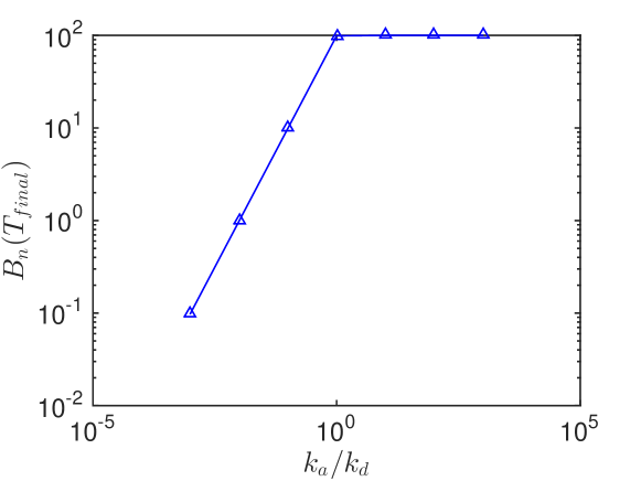
Figure 4: The population of ${\rm B}_{n}$ at stable state under the stochastic Hill function system with respect to different $k_{a}/k_{d}$ values, where $k_{d}=1$.

5.2 Two parameter case

This subsection studies the two parameter case, in which $k_{a}$ and $k_{d}$ are unknown while $\sigma=2$ and $k_{m}=100$ in the stochastic Hill function system. The QNSTOP settings are: total iterations = 100, sample point number $N=10$, initial ellipsoid radius $\hbox{TAU}=0.85$ (one-tenth of the $[L,U]$ box diameter), ellipsoid radius $\tau_{k}$ decay factor $\hbox{GAIN}=35$, $\hbox{MODE}=\hbox{`G'}$ (global optimization mode). There are $m=50$ empirical data points collected at time step $\tau=0.2$ from one SSA simulated trajectory of the ${\rm B}_{n}$ population. The $\alpha$-$\beta$-$\gamma$ acceptable region is defined by $\alpha=0.2$, $\beta=0.8$, $\gamma=0.2$, which indicates that 80% of the sampled values should have objective function values within 20% relative error of the local minimum, and the local minimum is within 20% relative error of the lowest minimum found over all starting points and iterations.

Fig. 5 shows the objective function values of maximum log-likelihood ($f_{l}$) over the entire $k_{a}$, $k_{d}$ domain. In the center of the graph, the dark blue region ($\log_{10}(k_{a})\in[-1,0]$, $\log_{10}(k_{d})\in[-2,0]$) has the minimum objective function value, $f_{l}\approx 500$. Any ($\log_{10}(k_{a})$, $\log_{10}(k_{d})$) pairs sampled in the dark blue region are acceptable values for the stochastic Hill function system (3).

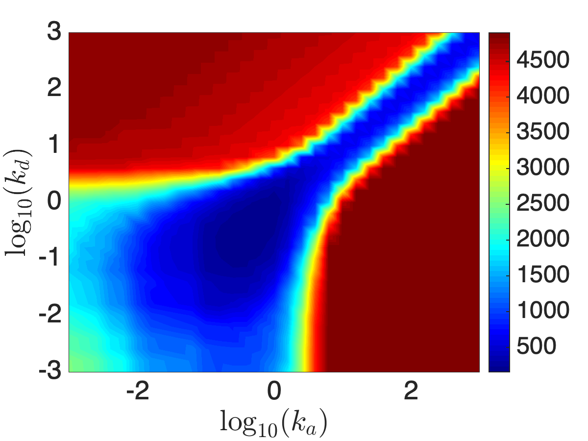
Figure 5: Exhaustive search of objective function values from the maximum log-likelihood method over domain $(\log_{10}(k_{a}),\log_{10}(k_{d}))\in[-3,3]^{2}$.

Influence of starting points. Fig. 6 shows the execution traces of QNSTOP and the corresponding acceptable parameter regions from different starting points: lower boundary point $L$, upper boundary point $U$, and center point $(L+U)/2$. There are three types of execution traces in Fig. 6(a, c, e): the solid red line is the objective function values of the ellipsoid center at each iteration; the dashed blue line is the minimum objective function values sampled in the ellipsoidal region of each iteration; the dotted black line is the maximum objective function values sampled in the ellipsoidal region of each iteration. From the execution traces of all three starting points, the best sampled objective function value $f_{l}(X)$ decreases fast in the first 20 iterations and then oscillates around 200. The worst sampled objective function value also oscillates around 200 after 60 iterations. In Fig. 6(b, d, f), all ellipsoids satisfying the $\alpha$-$\beta$-$\gamma$ rule, which form the acceptable region of parameter space, are plotted in the domain. The acceptable parameter regions are similar for all three methods and are located in the range of $[-1,0.5]$ for both $\log_{10}(k_{a})$ and $\log_{10}(k_{d})$, regardless of the subtle differences in region size and number of acceptable ellipsoids. Since QNSTOP can choose multiple random starting points from a Latin Hypercube experimental design, the rest of the paper shows the acceptable parameter regions collected from 20 such starting points.

Influence of empirical data. To study the robustness of the algorithm, vary the empirical data and the data size. Fig. 7 illustrates the acceptable regions from the same population trajectory of ${\rm B}_{n}$ but with different numbers of data points. Fig. 7(a) samples ten data points of ${\rm B}_{n}$ population with a time step $\tau=1$, while Fig. 7(b),(c) sample 50 and 200 data points with time steps $\tau=0.2$ and $\tau=0.05$, respectively. The acceptable region of parameter space increases with the data size $m$.

Fig. 8 shows the optimization results from three different empirical datasets of ${\rm B}_{n}$ population trajectories sampled from the stochastic multisite phosphorylation system. With different population trajectories, the acceptable parameter regions are consistent in size and shape. Thus, the parameter optimization of the stochastic Hill function system is more sensitive to the size of dataset than the data content variation.

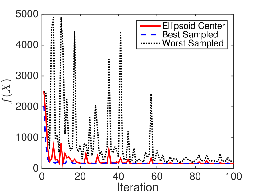
(a) Execution trace of QNSTOP

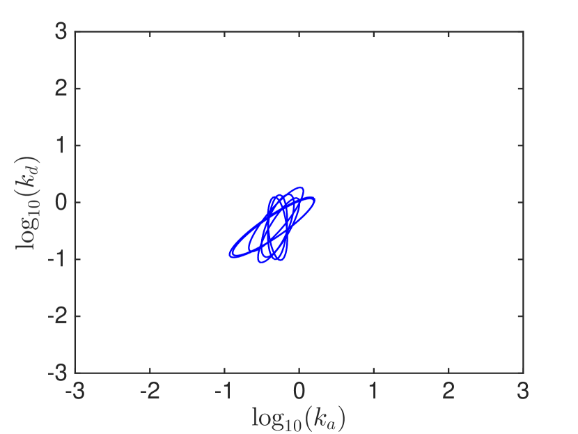
(b) Acceptable region

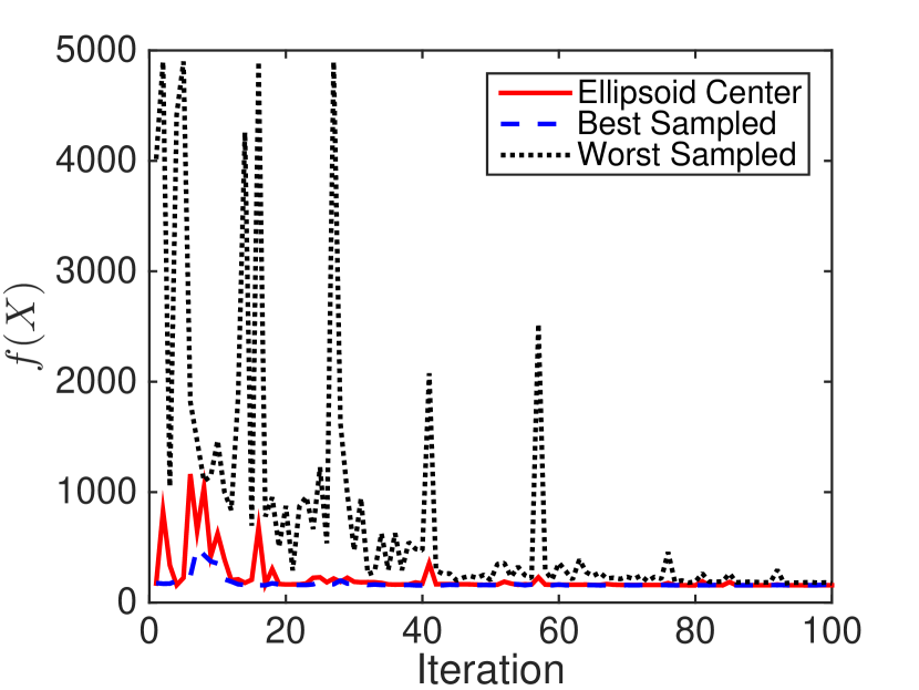
(c) Execution trace of QNSTOP

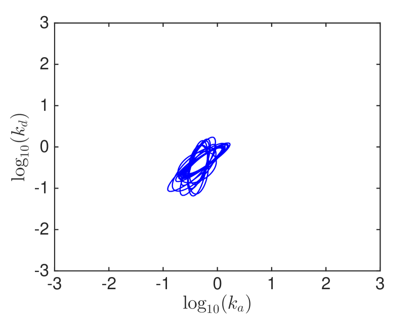
(d) Acceptable region

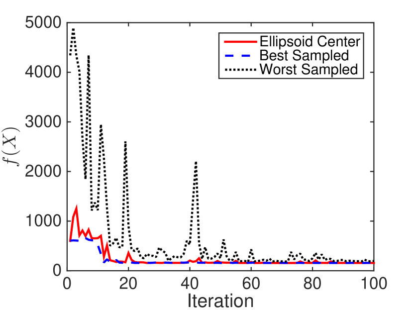
(e) Execution trace of QNSTOP

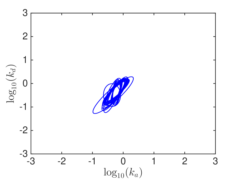
(f) Acceptable region

Figure 6: Execution traces of QNSTOP (left column) and acceptable regions of parameter space (right column) from maximum log-likelihood method with different starting points: (a, b) the lower box corner $(\log_{10}(k_{a}),\log_{10}(k_{d}))=(-3,-3)$; (c, d) box center $(\log_{10}(k_{a}),\log_{10}(k_{d}))=(0,0)$; (e, f) the upper box corner $(\log_{10}(k_{a}),\log_{10}(k_{d}))=(3,3)$. The three types of execution traces are: objective function values of the ellipsoid center at each iteration (red line); minimum objective function values sampled in the ellipsoidal region of each iteration (dashed blue line); maximum objective function values sampled in the ellipsoidal region of each iteration (dotted black line).

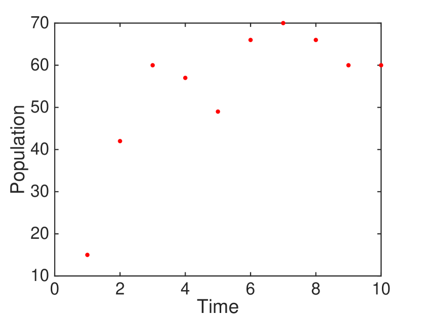
(a) Empirical data of ${\rm B}_{n}$ population

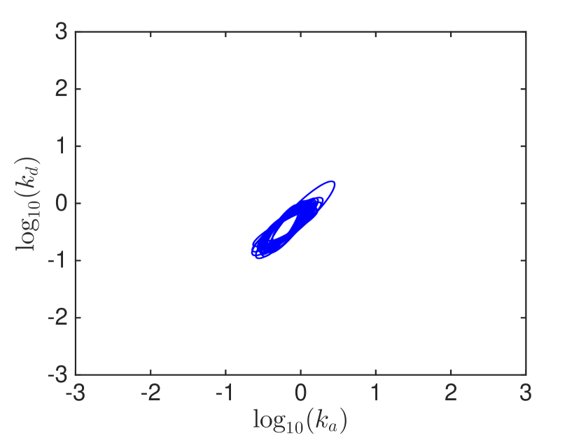
(b) Acceptable region

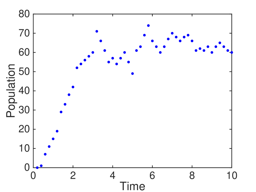
(c) Empirical data of ${\rm B}_{n}$ population

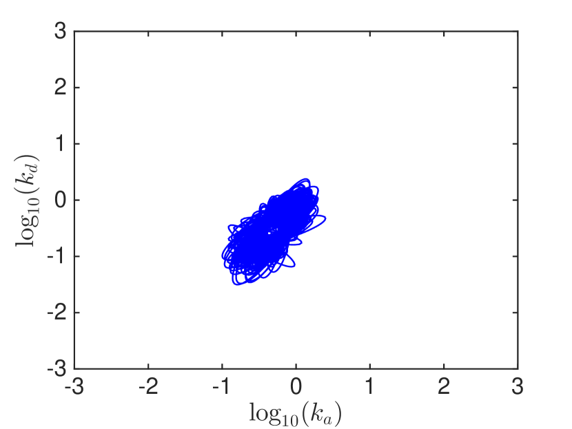
(d) Acceptable region

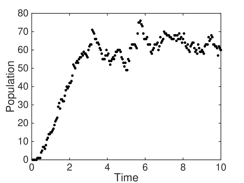
(e) Empirical data of ${\rm B}_{n}$ population

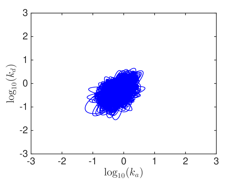
(f) Acceptable region

Figure 7: Different empirical data of ${\rm B}_{n}$ population (left column) and the corresponding acceptable parameter region (right column) from maximum log-likelihood method. The empirical data are sampled using different time steps $\tau$ and sample sizes $m$: (a, b) $\tau=1$, $m=10$; (c, d) $\tau=0.2$, $m=50$; (e, f) $\tau=0.05$, $m=200$. The acceptable parameter region is the union of results from 20 starting points.

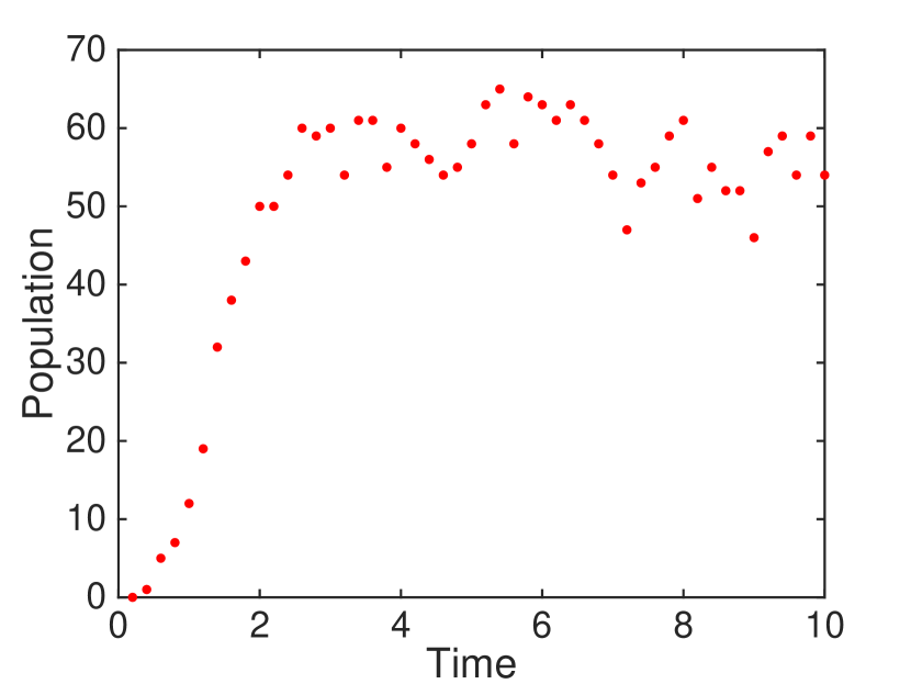
(a) Empirical data of ${\rm B}_{n}$ population

(b) Acceptable region

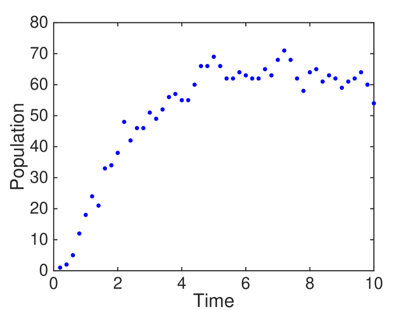
(c) Empirical data of ${\rm B}_{n}$ population

(d) Acceptable region

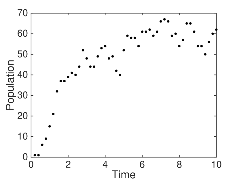
(e) Empirical data of ${\rm B}_{n}$ population

(f) Acceptable region

Figure 8: Optimization results of maximum log-likelihood with three different empirical data sets containing 50 data points, collected every 0.2 time unit. The acceptable region is the union of results from 20 starting points.

5.3 Full parameter case

This subsection studies the full parameter vector, in which all four parameters $k_{a}$, $k_{d}$, $\sigma$, and $k_{m}$ are unknown in the stochastic Hill function system. The QNSTOP settings are the same except the initial ellipsoid radius $\hbox{TAU}=1.3$ and the sample point number $N=20$. The empirical data is one simulated trajectory of the ${\rm B}_{n}$ population where $m=50$, $\tau=0.2$. The values of $\alpha\hbox{-}\beta\hbox{-}\gamma$ defining the acceptable regions are set differently according to the objective functions.

Influence of objective functions. Fig. 9 presents the results of the three objective functions: minimum distance area, maximum log-likelihood, and approximate maximum log-likelihood. For all three methods, the acceptable regions for the ($\log_{10}(k_{a})$, $\log_{10}(k_{d})$) pair are an ellipsoid shape centered at the middle of the domain, though the size has subtle differences. While for the ($\log_{10}(k_{m})$, $\log_{10}(\sigma)$) pair, the acceptable regions are all over the domain, shown in Fig. 10a. This results happens to all three methods, indicating that the system is not sensitive to parameters $k_{m}$, $\sigma$. Note that here the population level of enzyme A is fixed in this stochastic Hill function. The acceptable regions of the pair ($\log_{10}(k_{m})$, $\log_{10}(\sigma)$) will be significantly different if considering multiple population levels of enzyme A. Fig. 10b shows the results for an objective function that sums over 11 population levels of enzyme A, where $[{\rm A}]=150$, 300, 400, 520, 620, 800, 1050, 1400, 2100, 5000, 20000. This summed objective function will be explored in future work.

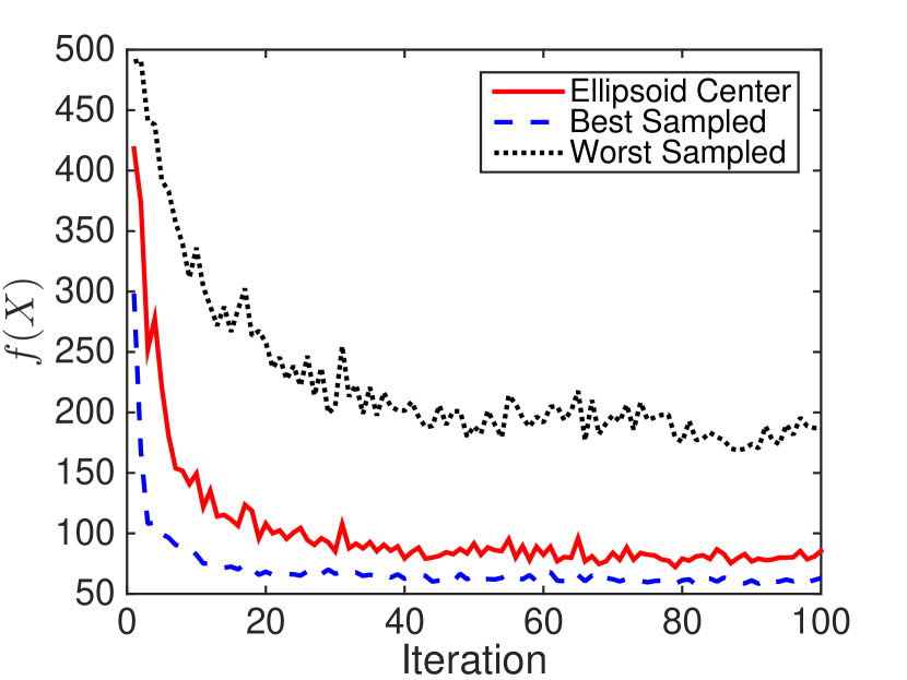
(a) Average execution trace of QNSTOP

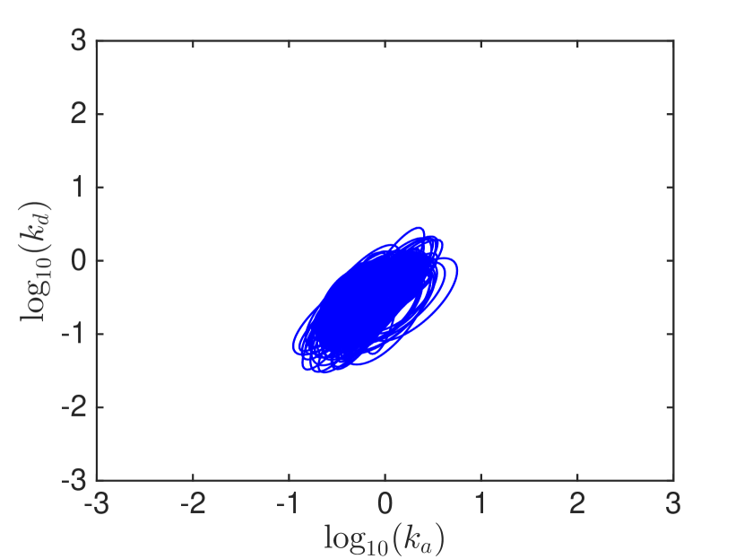
(b) Acceptable region

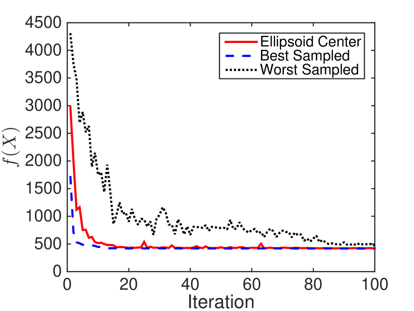
(c) Average execution trace of QNSTOP

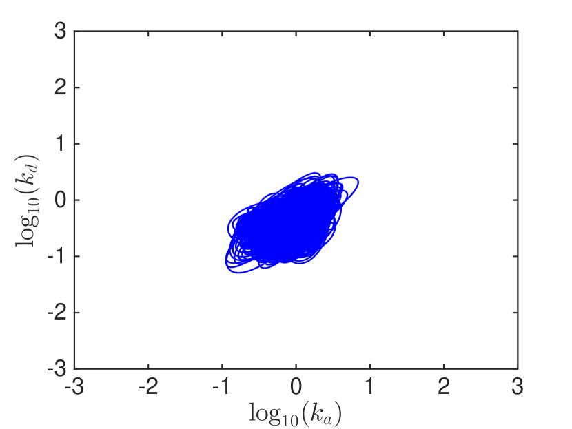
(d) Acceptable region

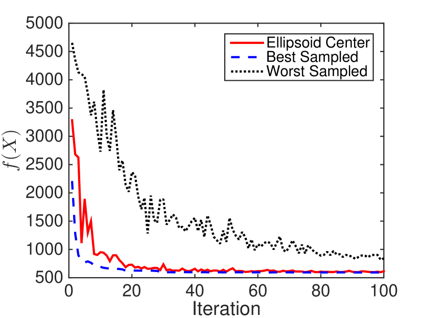
(e) Average execution trace of QNSTOP

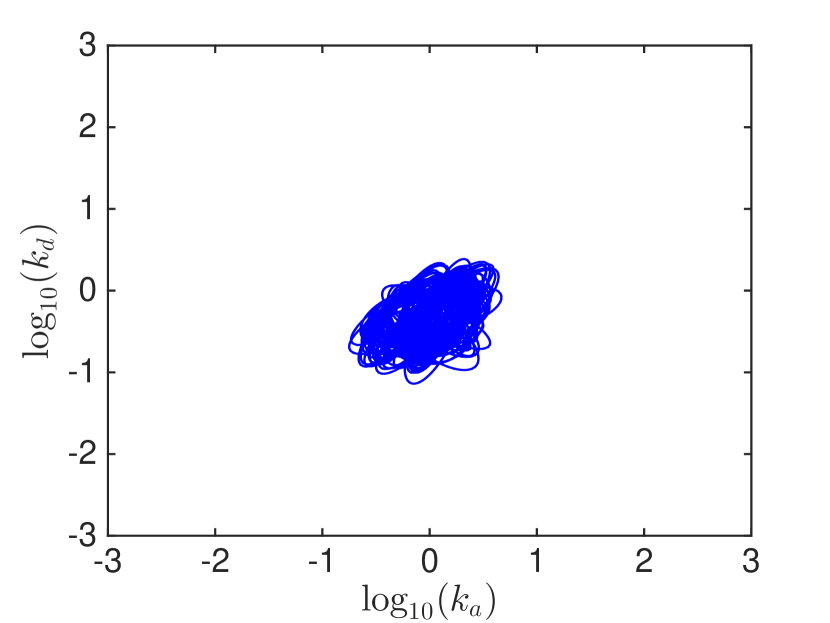
(f) Acceptable region

Figure 9: Average execution traces of QNSTOP (left column) based on 20 starting points and the corresponding acceptable parameter regions (right column) projected to two-dimensional domains of $k_{a}$ and $k_{d}$. (a, b) minimum distance area, (c, d) maximum log-likelihood, (e, f) approximate maximum log-likelihood.

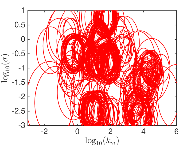
(a) Acceptable region for $k_{m},\sigma$

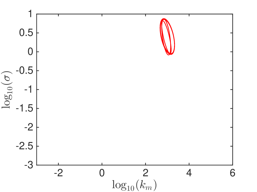
(b) Acceptable region for $k_{m},\sigma$

Figure 10: Acceptable parameter regions projected to two-dimensional domains of $k_{m}$ and $\sigma$ from maximum log-likelihood method. (a) The population of enzyme A is fixed at a single value. (b) 11 population levels of enzyme A are considered in the stochastic Hill function system.

To compare the stochastic Hill function system with the ordered distributive enzyme-substrate phosphoryaltion process, sample 100 points from the returned acceptable parameter region. Fig. 11 shows the average population trajectory of ${\rm B}_{n}$ in the stochastic Hill function using the sampled parameter values. The average population dynamics from all three methods match well with the empirical data. Fig. 12 further demonstrates the population distributions of the stochastic Hill function system based on the 100 parameter vector values sampled from the acceptable regions. Except for the significant difference at the initial stage of the ${\rm B}_{n}$ transition (time $t<1$), the empirical data falls in the 25th-75th percentile range for other stages (time $t=2$, $t=3$, $t=6$, $t=8$, $t=10$) from maximum log-likelihood and approximate maximum log-likelihood methods. The 25th-75th percentile range of ${\rm B}_{n}$ population from minimum distance area is narrower than that from the other two methods.

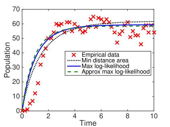
Figure 11: Average population dynamics of ${\rm B}_{n}$ in the stochastic Hill function system based on 100 parameter vector values sampled from the acceptable regions returned by minimum distance area, maximum log-likelihood, and approximate maximum log-likelihood. The simulated empirical data (50 data points) are marked by red crosses.

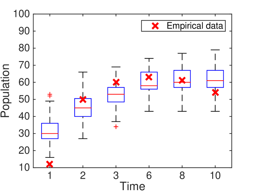
(a) Minimum distance area

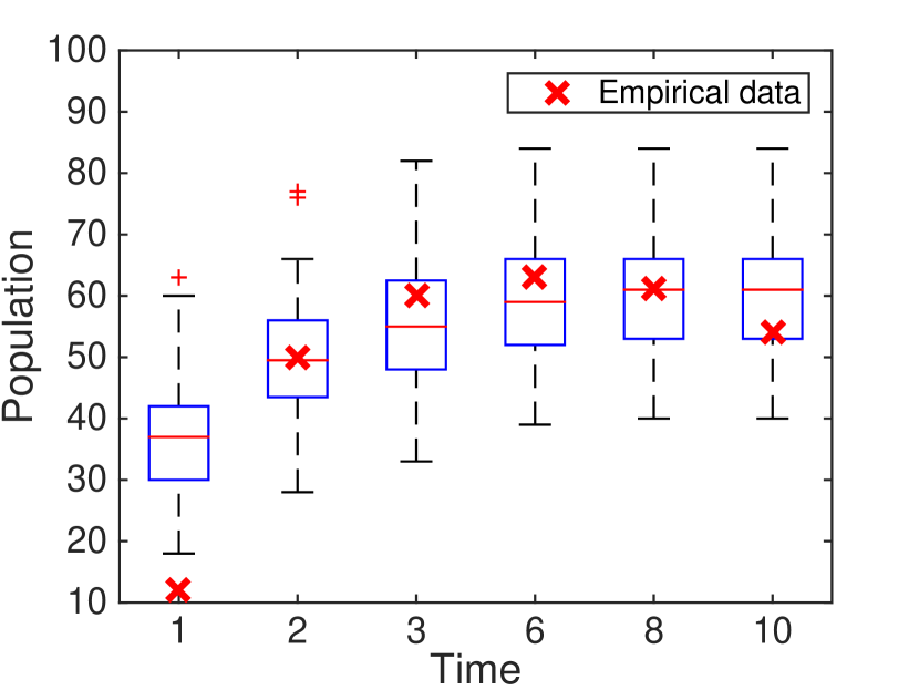
(b) Maximum log-likelihood

(c) Approximate maximum log-likelihood

Figure 12: Population distributions of ${\rm B}_{n}$ in the stochastic Hill function system (3) at time $t=1$, 2, 3, 6, 8, 10, corresponding to 10%, 20%, 30%, 60%, 80%, 100% of the total simulation time, based on 100 points sampled in each acceptable parameter region from minimum distance area, maximum log-likelihood, and approximate maximum log-likelihood.

6 Conclusion

This paper formulated a stochastic Hill function model for the multisite phosphorylation mechanism, and matched SSA simulation-based empirical population trajectory data for the ordered distributive enzyme-substrate phosphorylation process, using three different objective functions — minimum distance area, maximum log-likelihood, and approximate maximum log-likelihood. The approximate maximum log-likelihood method works well and is applicable to large complex biochemical networks. The main contributions are (1) an $\alpha$-$\beta$-$\gamma$ rule to find acceptable parameter regions instead of a single best parameter vector, (2) the Hill function system model must be matched to data with varying enzyme levels [A], and (3) demonstrating again that QNSTOP is well-suited to stochastic biological system model parameter estimation. Results showed that the optimized stochastic Hill function can be used to model the switch behavior and the steady state of the multisite phosphorylation process, while it cannot capture the initial transition period. QNSTOP and the $\alpha\hbox{-}\beta\hbox{-}\gamma$ rule are generally applicable to other stochastic models. Meanwhile, for aforementioned first order reaction networks where theoretical solution or efficient modeling and simulation methods of the stochastic kinetics are available, one may take advantage of these theoretical solutions or reduced models and develop more efficient parameter estimation strategies.

References

- [1] G. S. Adair. The hemoglobin system VI. The oxygen dissociation curve of hemoglobin. Journal of Biological Chemistry, 63(2):529–545, 1925.
- [2] F. Ali, C. Hindley, G. McDowell, R. Deibler, A. Jones, M. Kirschner, F. Guillemot, and A. Philpott. Cell cycle-regulated multi-site phosphorylation of neurogenin 2 coordinates cell cycling with differentiation during neurogenesis. Development, 138(19):4267–4277, 2011.
- [3] B. D. Amos, D. R. Easterling, L. T. Watson, W. I. Thacker, B. S. Castle, and M. W. Trosset. Algorithm XXX: QNSTOP—quasi-Newton algorithm for stochastic optimization. Technical report, TR-14-02, Department of Computer Science, Virginia Polytechnic Institute & State University, Blacksburg, VA, 2014.
- [4] M. Ashyraliyev, Y. Fomekong-Nanfack, J. A. Kaandorp, and J. G. Blom. Systems biology: parameter estimation for biochemical models. The FEBS journal, 276(4):886–902, 2009.
- [5] D. Barik, W. T. Baumann, M. R. Paul, B. Novak, and J. J. Tyson. A model of yeast cell-cycle regulation based on multisite phosphorylation. Molecular systems biology, 6(1), 2010.
- [6] F. L. Brown. Single-molecule kinetics with time-dependent rates: a generating function approach. Physical review letters, 90(2):028302, 2003.
- [7] S. L. Brunton, J. L. Proctor, and J. N. Kutz. Discovering governing equations from data by sparse identification of nonlinear dynamical systems. Proceedings of the National Academy of Sciences, 113(15):3932–3937, 2016.
- [8] B. Castle. Quasi-Newton methods for stochastic optimization and proximity-based methods for disparate information fusion. PhD thesis, Indiana University, 2012.
- [9] M. Chen, B. D. Amos, L. T. Watson, J. J. Tyson, Y. Cao, C. A. Shaffer, M. W. Trosset, C. Oguz, and G. Kakoti. Quasi-Newton stochastic optimization algorithm for parameter estimation of a stochastic model of the budding yeast cell cycle. IEEE/ACM transactions on computational biology and bioinformatics, 16(1):301–311, 2017.
- [10] M. Chen, Y. Cao, and L. T. Watson. Parameter estimation of stochastic models based on limited data. ACM SIGBioinformatics Record, 7(3):3, 2018.
- [11] M. Chen, F. Li, S. Wang, and Y. Cao. Stochastic modeling and simulation of reaction-diffusion system with hill function dynamics. BMC systems biology, 11(3):21, 2017.
- [12] I. Darvey and P. Staff. Stochastic approach to first-order chemical reaction kinetics. The Journal of Chemical Physics, 44(3):990–997, 1966.
- [13] D. R. Easterling, L. T. Watson, M. L. Madigan, B. S. Castle, and M. W. Trosset. Parallel deterministic and stochastic global minimization of functions with very many minima. Computational Optimization and Applications, 57(2):469–492, 2014.
- [14] J. E. Ferrell, S. H. Ha, et al. Ultrasensitivity part ii: multisite phosphorylation, stoichiometric inhibitors, and positive feedback. Trends in biochemical sciences, 39(11):556–569, 2014.
- [15] Z. Fox, G. Neuert, and B. Munsky. Finite state projection based bounds to compare chemical master equation models using single-cell data. The Journal of chemical physics, 145(7):074101, 2016.
- [16] C. Gadgil, C. H. Lee, and H. G. Othmer. A stochastic analysis of first-order reaction networks. Bulletin of mathematical biology, 67(5):901–946, 2005.
- [17] C. Gérard, J. J. Tyson, and B. Novák. Minimal models for cell-cycle control based on competitive inhibition and multisite phosphorylations of cdk substrates. Biophysical journal, 104(6):1367–1379, 2013.
- [18] D. T. Gillespie. A general method for numerically simulating the stochastic time evolution of coupled chemical reactions. Journal of computational physics, 22(4):403–434, 1976.
- [19] D. T. Gillespie. A rigorous derivation of the chemical master equation. Physica A: Statistical Mechanics and its Applications, 188(1-3):404–425, 1992.
- [20] A. V. Hill. The possible effects of the aggregation of the molecules of haemoglobin on its dissociation curves. j. physiol., 40:4–7, 1910.
- [21] O. Kapuy, D. Barik, M. R. D. Sananes, J. J. Tyson, and B. Novák. Bistability by multiple phosphorylation of regulatory proteins. Progress in biophysics and molecular biology, 100(1-3):47–56, 2009.
- [22] D. Koshland Jr, G. Nemethy, and D. Filmer. Comparison of experimental binding data and theoretical models in proteins containing subunits. Biochemistry, 5(1):365–385, 1966.
- [23] G. Lente. Stochastic mapping of first order reaction networks: A systematic comparison of the stochastic and deterministic kinetic approaches. The Journal of chemical physics, 137(16):164101, 2012.
- [24] X. Liu and M. Niranjan. State and parameter estimation of the heat shock response system using kalman and particle filters. Bioinformatics, 28(11):1501–1507, 2012.
- [25] X. Liu and M. Niranjan. Parameter estimation in computational biology by approximate bayesian computation coupled with sensitivity analysis. arXiv preprint arXiv:1704.09021, 2017.
- [26] M Chen, S Wang, and Y Cao. Accuracy analysis of hybrid stochastic simulation algorithm on linear chain reaction systems. Bulletin of Mathematical Biology, 81(8):3024–3052, 2019.
- [27] P. Mendes and D. Kell. Non-linear optimization of biochemical pathways: Applications to metabolic engineering and parameter estimation. Bioinformatics (Oxford, England), 14(10):869–883, 1998.
- [28] J. Monod, J. Wyman, and J.-P. Changeux. On the nature of allosteric transitions: a plausible model. J Mol Biol, 12(1):88–118, 1965.
- [29] B. Munsky and M. Khammash. The finite state projection algorithm for the solution of the chemical master equation. The Journal of chemical physics, 124(4):044104, 2006.
- [30] L. Pauling. The oxygen equilibrium of hemoglobin and its structural interpretation. Proceedings of the National Academy of Sciences of the United States of America, 21(4):186, 1935.
- [31] N. R. Radcliffe, D. R. Easterling, L. T. Watson, M. L. Madigan, and K. A. Bieryla. Results of two global optimization algorithms applied to a problem in biomechanics. In Proceedings of the 2010 Spring Simulation Multiconference, page 86. Society for Computer Simulation International, 2010.
- [32] A. Raj and A. van Oudenaarden. Single-molecule approaches to stochastic gene expression. Annual review of biophysics, 38:255–270, 2009.
- [33] C. Robert and G. Casella. Monte Carlo statistical methods. Springer Science & Business Media, 2013.
- [34] B. Y. Rubinstein, H. H. Mattingly, A. M. Berezhkovskii, and S. Y. Shvartsman. Long-term dynamics of multisite phosphorylation. Molecular biology of the cell, 27(14):2331–2340, 2016.
- [35] S. H. Rudy, S. L. Brunton, J. L. Proctor, and J. N. Kutz. Data-driven discovery of partial differential equations. Science Advances, 3(4):e1602614, 2017.
- [36] C. Salazar and T. Höfer. Multisite protein phosphorylation–from molecular mechanisms to kinetic models. The FEBS journal, 276(12):3177–3198, 2009.