Simulation Models for Aggregated Data Meta-Analysis: Evaluation of Pooling Effect Sizes and Publication Biases.

Abstract

Simulation studies are commonly used to evaluate the performance of newly developed meta-analysis methods. For methodology that is developed for an aggregated data meta-analysis, researchers often resort to simulation of the aggregated data directly, instead of simulating individual participant data from which the aggregated data would be calculated in reality. Clearly, distributional characteristics of the aggregated data statistics may be derived from distributional assumptions of the underlying individual data, but they are often not made explicit in publications. This paper provides the distribution of the aggregated data statistics that were derived from a heteroscedastic mixed effects model for continuous individual data. As a result, we provide a procedure for directly simulating the aggregated data statistics. We also compare our distributional findings with other simulation approaches of aggregated data used in literature by describing their theoretical differences and by conducting a simulation study for three meta-analysis methods: DerSimonian and Laird’s pooled estimate and the Trim & Fill and PET-PEESE method for adjustment of publication bias. We demonstrate that the choices of simulation model for aggregated data may have a relevant impact on (the conclusions of) the performance of the meta-analysis method. We recommend the use of multiple aggregated data simulation models for investigation of new methodology to determine sensitivity or otherwise make the individual participant data model explicit that would lead to the distributional choices of the aggregated data statistics used in the simulation.

1 Introduction

An aggregated data meta-analysis would collect the information $(D_{i},S_{i},df_{i})$ for study $i,$ with $D_{i}$ the estimated study effect size of interest (e.g., mean difference, Cohen’s $d$, log odds ratio), $S_{i}$ the estimated standard error of the study effect size, and $df_{i}$ the corresponding degrees of freedom for the standard error Cochran1954 . The aggregated data is typically constructed from individual data (although a researcher may not have access to this individual data). The aggregated data is then used to determine a pooled estimate of the main effect size and to calculate other aspects related to the quality of the meta-analysis (e.g., measure of heterogeneity, publication bias, sensitivity analyses).

To investigate the performance of meta-analysis methods, researchers often resort to simulation of the aggregated data $(D_{i},S_{i},df_{i})$ directly, making certain distributional assumptions Brockwell2001 ; Chung2013 ; Rukhin2013 ; Ning2017 . The distribution of $D_{i}$ is typically assumed normal and the standard error $S_{i}$ is often related to a chi-square distribution. jackson_when_2018 While these distributional assumptions may be plausible, the choices are not properly supported or defended by an underlying statistical model on the individual data that would generate the aggregated data, making it difficult to understand if the simulation model for the aggregated statistics represents the practice appropriately. On the other hand, when individual data is being simulated Stanley2008 ; Stanley2014 ; Alinaghi2018 there is limited discussion on the distributional characteristics of the aggregated data $(D_{i},S_{i},df_{i})$. This makes it difficult to compare simulations on an individual level with simulations conducted at the aggregated level and it is hard to verify the compliance of the distribution of the aggregated statistics in practice with the induced distributional assumptions of the individual data. Furthermore, research papers often choose but one simulation approach and it is typically unknown how well the conclusions of this single simulation model would hold for other choices of simulation.

This paper discusses a (fixed and random effects) heteroscedastic mixed effects model for a continuous outcome at an individual level where two groups (e.g., treatments) are being compared. The model assumes three forms of heterogeneity. The first form is a bivariate random effect on the two mean outcomes across studies, indicating heterogeneity in outcome level between individuals across studies. The second form is a fixed heteroscedastic residual error for the two groups within a study, implying that inter-individual variability within studies can depend on other variables (like treatment). The third form is a random heteroscedastic residual error across studies, which would represent that inter-individual variability can also change with studies due to the selection of more homogeneous or heterogeneous participants. We believe that this model has not been discussed for meta-analysis purposes so far. Based on this model we will discuss distributional properties of the aggregated data $(D_{i},S_{i},df_{i})$, which is useful to be able to simulate study data at an aggregated level directly.

These distributional properties will be compared with similar distributional properties of certain other aggregated data simulation models from literature to investigate the plausibility of these choices. Secondly, we will conduct a simulation study to investigate the impact of different distributional choices on some well-known meta-analysis approaches. We selected the very popular pooled estimation method of DerSimonian and Laird for the random effects meta-analysis model DerSimonian1986 , the popular Trim & Fill method Duval2000 ; Duval2000a for adjustments of publication bias in meta-analysis practice Dadi2020 ; Liu2020 ; Torous2020 , and the PET-PEESE approach Stanley2008 ; Stanley2014 also for adjustment of publication bias. The PET-PEESE method has been popular in at least the economics field Alinaghi2018 .

In section 2 we describe a selection of aggregated data simulation models we have encountered in literature. In section 3, we propose a statistical model for individual participant data and determine distributional properties of the corresponding aggregated statistics. We also provide a simulation procedure to simulate aggregated data according to this model. We discuss the differences between our approach with the selected models from the literature as well. The fourth section presents a simulation study where the aggregated data simulation models are being compared. We also provide the simulation settings and a selection model for publication bias used in literature as well. Then finally we provide a discussion of the results in Section 6.

2 Simulation of Aggregated Data in Literature

In this section we will provide an overview of a few simulation models that we have encountered in literature to support investigations of the performance of meta-analysis approaches. The simulation models used in literature all uses the well-known random effects model DerSimonian1986 ; Hardy1996 for the study effect size $D_{i}$ at the aggregated level that is given by

$$D_{i}=\theta+U_{i}+\varepsilon_{i},$$ (1)

with $\theta$ the mean study effect of interest, $U_{i}\sim\mathcal{N}(0,\tau^{2})$ a random effect for study $i$ to accommodate study heterogeneity on the treatment effect (i.e., $\theta+U_{i}$ is the effect size for study $i$), $\varepsilon_{i}\sim\mathcal{N}(0,\sigma_{i}^{2})$ the residual for study $i$, and $U_{i}$ and $\varepsilon_{i}$ independent. Thus, $D_{i}$ is created by drawing $U_{i}$ and $\varepsilon_{i}$ for study $i$.

Simulations at the aggregated level also have to generate estimators $S_{i}^{2}$ for the variance component $\sigma_{i}^{2}$ of the residual. Differences between the aggregated data simulation models in literature are typically determined by the choice of distribution function for the standard deviation $S_{i}$. The choice of distributions have been the central chi-square for $S_{i}^{2}$ in Sidik and Jonkman Sidik2002 and Brockwell and Gordon Brockwell2001 , the non-central chi-square for $S_{i}^{2}$ in Ning et al. Ning2017 , and the gamma distribution for $S_{i}$ in Duval and Tweedie Duval2000a . All these aggregated data simulation models assume that $\sigma_{i}^{2}=\mathsf{VAR}(\varepsilon_{i}|S_{i}^{2})=S_{i}^{2}$, indicating that $S_{i}^{2}$ is drawn first before the study effect $D_{i}$ is simulated. Furthermore, the size of a study, which may be represented by the degrees of freedom $df_{i}$ of $S_{i}^{2}$, is not considered as a separate measure by these simulation models.

2.1 Central Chi-Square Distributed $S_{i}^{2}$

For the simulation of log odds ratios in an aggregated data meta-analysis, Brockwell and Gordon Brockwell2001 and Sidik and Jonkman Sidik2002 simulated the log odds ratio $D_{i}$ according to model (1). Here $S_{i}^{2}$ is selected to be equal to $S_{i}^{2}=0.25\chi_{i}^{2}$, with $\chi_{i}^{2}$ a chi-square distributed random variable having only one degrees of freedom (thus effectively choosing $df_{i}=1$). They also restricted the value of $S_{i}^{2}$ to be within $(0.009,0.6)$ to conform with a typical distribution of the variances of log odds-ratios in practice Brockwell2001 ; Sidik2002 . For mean differences we do not think that we should implement these variance restrictions. In their comparisons of several meta-analysis methods of pooling log odd ratios they did not make use of the $df_{i}$ in any way. They selected a mean study effect of $\theta=0.5$ and evaluated eleven different values for the heterogeneity $\tau^{2}$ in the range of $0$ to $0.1$.

2.2 Non-Central Chi-Square Distributed $S_{i}^{2}$

For an investigation of a publication bias method, Ning et al., Ning2017 simulated the study effect size $D_{i}$ according to model (1) with condition $\mathsf{VAR}(\varepsilon_{i}|S_{i}^{2})=S_{i}^{2}$. And to create the variance $S_{i}^{2}$, they draw a normally distributed random variable $Z_{i}\sim N(0.25,0.5)$ and calculated the variance by $S_{i}^{2}=Z_{i}^{2}$. The distribution of this variance is equal to a non-central chi-square distribution with non-centrality parameter equal to $1/8$ ($=(0.25)^{2}/0.5$). They did not implement the degrees of freedom $df_{i}$.The mean effect size was taken equal to $\theta=0.4$ and the heterogeneity was selected equal to $\tau=0.5$ and $\tau=1$.

2.3 Gamma Distributed $S_{i}$

For an investigation of the Trim & Fill method for publication bias, Duval and Tweedie Duval2000 ; Duval2000a simulated the study effect size $D_{i}$ according to model (1) with a standard error $S_{i}$ drawn from a Gamma distribution with parameters $3$ and $1/9$ (i.e., $S_{i}\sim\Gamma(3,1/9)$). Their argument for this choice is that it provides a more typical funnel plot than a uniform distribution for $S_{i}$, which was applied by Light and Pillemer Light1986 . They did not specify which parametrization of the gamma distribution they selected, but we guess that the mean of $S_{i}$ would be equal to $1/3$ ($=3\times 1/9$) and with a variance equal to $1/27$ ($=3\times(1/9)^{2}$), considering the values for precision $S_{i}^{-1}$ they used in their funnel plots. They assumed that both the mean study effect $\theta$ and heterogeneity $\tau^{2}$ were equal to zero.

3 Heteroscedastic Mixed Effects Model

Different data-generating mechanisms in simulation studies for meta-analysis may potentially affect the results when comparing the performances of different meta-analysis methods. In this section, we will describe an individual participant data (IPD) simulation model which allows treatment heterogeneity and heteroscedasticity across treatment arms and across trials. Furthermore, we will show that the distributional properties of the aggregated data $D_{i}$, $S_{i}^{2}$, and $df_{i}$ for a meta-analysis that we obtained from our heterogeneous and heteroscedastic IPD model deviates from what is normally used in literature.

Let $Y_{ijk}$ be a continuous outcome variable for individual $k=1,2,...,n_{ij}$ in treatment group $j=0,1$ for study $i=1,2,...,m$. Treatment $j=0$ represents the control group and treatment $j=1$ is the treatment under investigation. Note that we use treatment here, but it could be in principle any binary variable that splits the data in two groups (e.g., sex, symptom, disease). The statistical model is described as follows:

$$Y_{ijk}=\mu+\beta_{j}+U_{ij}+\varepsilon_{ijk}$$ (2)

with $\mu$ the mean response at the control group, $\beta_{0}=0$ for identifiability purposes, $\beta_{1}$ the mean treatment effect and typically the (association) parameter of interest, $U_{ij}$ the (latent) study heterogeneity for treatment group $j$, and $\varepsilon_{ijk}$ a potentially heteroscedastic residual. We will assume that the random elements are normally distributed, such that

$$\begin{array}[]{rcl}\varepsilon_{ijk}|V_{i}&\sim&\mathcal{N}(0,\sigma_{j}^{2}\exp\left\{V_{i}\right\}),\\ \left(U_{i0},U_{i1},V_{i}\right)^{T}&\sim&\mathcal{N}(\boldsymbol{0},\boldsymbol{\Sigma}),\end{array}$$ (3)

with $V_{i}$ a (latent) random heteroscedastic study effect on the residuals in (2), with $\boldsymbol{\Sigma}$ given by

$$\boldsymbol{\Sigma}=\left(\begin{array}[]{ccc}\tau_{0}^{2}&\rho_{01}\tau_{0}\tau_{1}&\rho_{02}\tau_{0}\tau_{2}\\ \rho_{01}\tau_{0}\tau_{1}&\tau_{1}^{2}&\rho_{12}\tau_{1}\tau_{2}\\ \rho_{02}\tau_{0}\tau_{2}&\rho_{12}\tau_{1}\tau_{2}&\tau_{2}^{2}\end{array}\right),$$

and $\varepsilon_{ijk}$ and $(U_{i0},U_{i1})$ being independent conditionally on $V_{i}$. It should be noted that our assumptions of normality are not uncommon for the analysis of clinical trials and observational studies Molenberghs2007 ; Rosenbaum2002 . Furthermore, heteroscedastic hierarchical models defined by (2) and (3) have been discussed in literature as well Davidian1987 ; Quintero2017 , but not in the context of meta-analysis.

Our model describes study heterogeneity ($U_{ij}$) on the mean response, indicating that the outcome level may vary with studies, but that this form of heterogeneity is not the same for both treatment groups. This may not be unrealistic when the treatment group would fully cure a disease but the control group does not, assuming that variability within a population is larger when it is composed of healthy and diseased individuals. It is this form of heterogeneity that leads to the (well-known) random effects meta-analysis model (1) at the aggregated level. When the heterogeneity would be identical for both treatment groups ($\rho_{01}=1$ and $\tau_{1}=\tau_{2}$), we may only observe heterogeneity at the individual level data for each treatment group, but not necessarily at the aggregated study effect (see Section 3.1).

Furthermore, we also assume that the residual variability, which represents inter-individual variability, is treatment dependent (i.e., $\sigma_{0}$ and $\sigma_{1}$ may be different). This is not uncommon in several areas of medicine (e.g., hypertension treatment) where treatment is not just affecting the level of the outcome in a population, but also its variability. Our model also describes a residual heteroscedasticity that is study dependent ($V_{i}$). This could be related to the selection of participants in a study, leading to a study with either more homogeneous or less homogeneous participants. For instance, a clinical trial with mostly men at a specific age group would show less inter-individual variability than a trial with both sexes and a larger variety in age groups. Combining these different trials in a meta-analysis results in a random residual heteroscedasticity. Here we assume that we do not have any complementary data to investigate or eliminate such heteroscedasticity, implying the necessity of $V_{i}$ in model (2).

Model (2) can be rewritten into $Y_{ijk}=\mu+\beta_{j}+U_{ij}+\sigma_{j}Z_{ijk}\exp\left\{0.5V_{i}\right\}$, with $Z_{ijk}$ i.i.d. standard normally distributed residuals (i.e., $Z_{ijk}\sim\mathcal{N}(0,1)$), which are independent of the random effects $U_{i0}$, $U_{i1}$, and $V_{i}$. This formulation demonstrates immediately that the selected model (2) with assumptions (3) has introduced a correlation between the residuals $\sigma_{j}Z_{ijk}\exp\left\{0.5V_{i}\right\}$ and the random location effects $(U_{i0},U_{i1})$. In case we choose $\rho_{02}=\rho_{12}=0$, the error structure in (2) and the study treatment heterogeneity $U_{ij}$ will be independent. It also shows that the marginal distribution of $Y_{ijk}$ is not normal anymore, due to the product of a normal and log normal random variable in the residual, unless $\tau_{2}=0$ of course.

Finally, the distribution of $U_{i1}-U_{i0}$ and $V_{i}$ is bivariate normally distributed with mean $\boldsymbol{0}$ and a variance-covariance matrix given by

$$\left(\begin{array}[]{cc}\tau_{0}^{2}-2\rho_{01}\tau_{0}\tau_{1}+\tau_{1}^{2}&\tau_{2}[\rho_{12}\tau_{1}-\rho_{02}\tau_{0}]\\ \tau_{2}[\rho_{12}\tau_{1}-\rho_{02}\tau_{0}]&\tau_{2}^{2}\end{array}\right).$$

The difference $U_{i1}-U_{i0}$ is important in Section 3.1 when we determine and discuss the study effect size $D_{i}$. The correlation coefficient $\rho$ between $U_{i1}-U_{i0}$ and $V_{i}$ is equal to $\rho=[\rho_{12}\tau_{1}-\rho_{02}\tau_{0}]/\sqrt{\tau_{0}^{2}-2\rho_{01}\tau_{0}\tau_{1}+\tau_{1}^{2}}$. We will demonstrate that the study effect size $D_{i}$ and its corresponding standard error $S_{i}$ will always be dependent even in the absence of correlation ($\rho=0$) between $U_{i1}-U_{i0}$ and $V_{i}$ (i.e., $\rho_{02}\tau_{0}=\rho_{12}\tau_{1}$), unless $\tau_{2}=0$ of course.

3.1 Aggregated Effects Sizes and Standard Errors

A popular effect size used in meta-analysis calculated for each study is the (raw) mean difference between the two treatment groups, i.e.,

$$D_{i}=\bar{Y}_{i1}-\bar{Y}_{i0},$$ (4)

with $\bar{Y}_{ij}=\sum_{k=1}^{n_{ij}}Y_{ijk}/n_{ij}$ the average response for study $i$ at treatment $j$. Using model (2), we can rewrite the effect size into

$$D_{i}=\beta_{1}+U_{i1}-U_{i0}+\exp\left\{0.5V_{i}\right\}\left[\sigma_{1}\bar{Z}_{i1}-\sigma_{0}\bar{Z}_{i0}\right],$$ (5)

with $\bar{Z}_{ij}=\sum_{k=1}^{n_{ij}}Z_{ijk}/n_{ij}$ the average standardized residuals for treatment $j$ in study $i$. Clearly, model (5) is identical to model (1), with $\theta=\beta_{1}$, $U_{i}=U_{i1}-U_{i0}$ and $\varepsilon_{i}=\exp\left\{0.5V_{i}\right\}\left[\tau_{1}\bar{Z}_{i1}-\tau_{0}\bar{Z}_{i0}\right]$, but the distributional assumptions on normality and independence only agree with our setting when the random heteroscedasticity vanishes (i.e., $\tau_{2}=0$). Under our model (5), the variances $\tau^{2}$ and $\sigma_{i}^{2}$ in model (1) would become equal to $\tau^{2}=\tau_{0}^{2}-2\rho_{01}\tau_{0}\tau_{1}+\tau_{1}^{2}$ and $\sigma_{i}^{2}=\exp\{\tau_{2}^{2}/2\}[\sigma_{0}^{2}/n_{i0}+\sigma_{1}^{2}/n_{i1}]$, respectively. The difference $U_{i1}-U_{i0}\sim N(0,\tau_{0}^{2}-2\rho_{01}\tau_{0}\tau_{1}+\tau_{1}^{2})$ represents the study heterogeneity of effect sizes, but it disappears when $\rho_{01}=1$ and $\tau_{0}=\tau_{1}$.

The conditional distribution of the effect size $D_{i}$, given the three random effects $U_{i0}$, $U_{i1}$, and $V_{i}$, is given by a normal distribution with mean $\beta_{1}+U_{i1}-U_{i0}$ and variance $\exp\left\{V_{i}\right\}\left[\sigma_{0}^{2}/n_{i0}+\sigma_{1}^{2}/n_{i1}\right]$. A larger study will demonstrate a smaller residual variance, since the sample sizes $n_{i0}$ and $n_{i1}$, which will then be smaller in other studies, will reduce the residual variance, but it could potentially be compensated by a larger inter-individual variability ($V_{i}>0$). However, we do not assume a direct relation between a positive value for $V_{i}$ and the sample size $n_{i0}$ and $n_{i1}$ (i.e., $P(V_{i}>0|n_{i0},n_{i1})=P(V_{i}>0)$). The conditional distribution of $D_{i}$ given only $V_{i}$ is also given by a normal distribution, but now with mean and variance given by

$$\begin{array}[]{rcl}\mathbb{E}(D_{i}|V_{i})&=&\beta_{1}+\tau_{2}^{-1}[\rho_{12}\tau_{1}-\rho_{02}\tau_{0}]V_{i},\\ \mathbb{\mathsf{VAR}}(D_{i}|V_{i})&=&(1-\rho_{02}^{2})\tau_{0}^{2}+2(\rho_{02}\rho_{12}-\rho_{01})\tau_{0}\tau_{1}+(1-\rho_{12}^{2})\tau_{1}^{2}\\ &&\qquad+\exp\left\{V_{i}\right\}\left[\sigma_{0}^{2}/n_{i0}+\sigma_{1}^{2}/n_{i1}\right].\end{array}$$ (6)

Finally, the marginal distribution function for $D_{i}$ is less tractable when $V_{i}$ is non-degenerative, since the distribution of the product of a log normal and a normal distributed random variable (i.e., $\exp\left\{0.5V_{i}\right\}\left[\sigma_{0}\bar{Z}_{i1}-\sigma_{1}\bar{Z}_{i0}\right]$) is unknown whether they are dependently or independently distributed (as we already mentioned for $Y_{ijk}$). However, we can determine the mean and variance of $D_{i}$ and they are given by

$$\begin{array}[]{rcl}\mathbb{E}(D_{i})&=&\beta_{1},\\ \mathbb{\mathsf{VAR}}(D_{i})&=&\tau_{0}^{2}-2\rho_{01}\tau_{0}\tau_{1}+\tau_{1}^{2}+\exp\left\{\tau_{2}^{2}/2\right\}[\sigma_{0}^{2}/n_{i0}+\sigma_{1}^{2}/n_{i1}].\end{array}$$ (7)

Note that correlation coefficient $\rho=[\rho_{12}\tau_{1}-\rho_{02}\tau_{0}]/\sqrt{\tau_{0}^{2}-2\rho_{01}\tau_{0}\tau_{1}+\tau_{1}^{2}}$ does not play a role in the variance of $D_{i}$, due to the independence of $U_{i1}-U_{i0}$ and $\sigma_{1}\bar{Z}_{i1}-\sigma_{0}\bar{Z}_{i0}$. Thus the variance is just the sum of the variance of the heterogeneity $U_{i1}-U_{i0}$ and the variance of the residual $\exp\left\{0.5V_{i}\right\}\left[\sigma_{1}\bar{Z}_{i1}-\sigma_{0}\bar{Z}_{i0}\right]$.

The estimated standard error $S_{i}$ for the effect size $D_{i}$ within one study (thus being unaware of any possible random effect $U_{i0}-U_{i1}$ across studies) can be estimated in different ways Borenstein2009 . If we do not want to make any assumptions on the equality of residual variances for the two treatment groups in model (2), it is most reasonable to estimate the standard error $S_{i}$ by $S_{i}^{2}=S_{i0}^{2}/n_{i0}+S_{i1}^{2}/n_{i1}$, with $S_{ij}^{2}=\sum_{k=1}^{n_{ij}}(Y_{ijk}-\bar{Y}_{ij})^{2}/(n_{ij}-1)$ the sample variance for treatment $j$ in study $i$. Using model (2), we can rewrite this sample variance $S_{ij}^{2}$ into $\sigma_{j}^{2}\exp\left\{V_{i}\right\}\chi_{ij}^{2}/(n_{ij}-1)$, with $\chi_{ij}^{2}=\sum_{k=1}^{n_{ij}}(Z_{ijk}-\bar{Z}_{ij})^{2}$ a chi-square distributed random variable with $n_{ij}-1$ degrees of freedom. Thus the variance $S_{i}^{2}$ is now distributed as

$$S_{i}^{2}=\exp\left\{V_{i}\right\}[\sigma_{0}^{2}\chi_{i0}^{2}/(n_{i0}(n_{i0}-1))+\sigma_{1}^{2}\chi_{i1}^{2}/(n_{i1}(n_{i1}-1))],$$ (8)

with an expectation equal to $\mathbb{E}(S_{i}^{2})=\exp\left\{\tau_{2}^{2}/2\right\}[\sigma_{0}^{2}/n_{i0}+\sigma_{1}^{2}/n_{i1}]$ and a variance equal to

$$\begin{array}[]{l}\mathsf{VAR}(S_{i}^{2})=2\exp\left\{2\tau_{2}^{2}\right\}\left[\sigma_{0}^{4}/(n_{i0}^{2}(n_{i0}-1))+\sigma_{1}^{4}/(n_{i1}^{2}(n_{i1}-1))\right]\\ \qquad\qquad\qquad\qquad\qquad+\exp\left\{\tau_{2}^{2}\right\}\left(\exp\left\{\tau_{2}^{2}\right\}-1\right)\left[\sigma_{0}^{2}/n_{i0}+\sigma_{1}^{2}/n_{i1}\right]^{2}.\end{array}$$ (9)

The random variable $\sigma_{0}^{2}\chi_{i0}^{2}/(n_{i0}(n_{i0}-1))+\sigma_{1}^{2}\chi_{i1}^{2}/(n_{i1}(n_{i1}-1))$ is approximately distributed as $[\sigma_{0}^{2}/n_{i0}+\sigma_{1}^{2}/n_{i1}]\chi_{df_{i}}^{2}/df_{i}$, with $\chi_{df_{i}}^{2}$ a chi-square distributed random variable with $df_{i}$ degrees of freedom. The number of degrees of freedom is given by Satterthwaite1946 ; Heuvel2010

$$df_{i}=\dfrac{\left[\sigma_{0}^{2}\chi_{i0}^{2}/(n_{i0}(n_{i0}-1))+\sigma_{1}^{2}\chi_{i1}^{2}/(n_{i1}(n_{i1}-1))\right]^{2}}{\sigma_{0}^{4}\chi_{i0}^{4}/\left[n_{i0}^{2}(n_{i0}-1)^{3}\right]+\sigma_{1}^{4}\chi_{i1}^{4}/\left[n_{i1}^{2}(n_{i1}-1)^{3}\right]}.$$ (10)

This number of degrees of freedom is bounded from above by $n_{i0}+n_{i1}-2$ and from below by $\min\left\{n_{i0}-1,n_{i1}-1\right\}$ Heuvel2010 . In case the sample sizes are equal ($n_{i0}=n_{i1}$) and the residual variances are equal ($\sigma_{0}^{2}=\sigma_{1}^{2}$), the random variable $\chi_{df_{i}}^{2}$ becomes chi-square with $df_{i}=n_{i0}+n_{i1}-2$ degrees of freedom. The distribution of $S_{i}^{2}$ in the general setting (8) using model (2) with assumptions (3) is clearly intractable, but becomes approximately equal to a chi-square distribution when $V_{i}$ becomes degenerate in zero.

The distribution of $S_{i}^{2}$ in (8) seems clearly different from those used in literature, since it is the distribution of a random variable that is a product of a lognormally distributed random variable and a weighted average of two chi-square distributed variables, where the weights depend on the sample sizes. Even if there is no residual heteroscedasticity ($\sigma_{0}=\sigma_{1}$ and $\tau_{2}=0$) and the sample sizes $n_{i0}$ and $n_{i1}$ are equal, $S_{i}^{2}$ has a central chi-square distribution with $df_{i}=n_{i0}+n_{i1}-2$ degrees of freedom and still deviates from the distributions for $S_{i}^{2}$ in Section 2. However, we have only studied the distribution function of $S_{i}^{2}$ conditionally on the sample sizes $n_{i0}$ and $n_{i1}$. In meta-analysis these sample sizes are typically known and could therefore be used in the analysis of a meta-analysis (e.g., by calculating appropriate degrees of freedom $df_{i}$), but for the central chi-square, the non-central chi-square, and gamma distributions in Section 2, these sample sizes are not being mentioned and, in a way, they can be viewed as distribution functions where the sample sizes have been integrated out (i.e., they essentially describe marginal distribution functions of $S_{i}^{2}$). Indeed, we do not know if there exist distribution functions for $n_{i0}$ and $n_{i1}$ that would make the marginal distribution of $S_{i}^{2}$ in (5) equal to any of the distribution functions in Section 2.

Note that $D_{i}$ and $S_{i}^{2}$ are independent conditionally on $V_{i}$, due to independence of the random variables $\chi_{i0}^{2}$, $\chi_{i1}^{2}$, $\bar{Z}_{i1}$, $\bar{Z}_{i1}$, and $U_{i0}-U_{i1}$. Here we have used the assumption of normality to obtain independence between the mean $\bar{Z}_{ij}$ and variance $S_{ij}^{2}$ (conditionally on $V_{i}$). Using this independence, (5), and (8), the joint distribution of $D_{i}$ and $S_{i}^{2}$ is now a mixture of the product of the two conditional distribution functions for $D_{i}|V_{i}$ and $S_{i}^{2}|V_{i}$. This implies that $D_{i}$ and $S_{i}^{2}$ are never independent, irrespective of the value of $\rho$, unless $V_{i}$ is degenerated. The covariance between $D_{i}$ and $S_{i}^{2}$ is equal to

$$\begin{array}[]{rcl}\mathtt{\mathsf{COV}}(D_{i},S_{i}^{2})&=&\mathbb{E}\left[(D_{i}-\beta_{1})S_{i}^{2}\right],\\ &=&\tau_{2}^{-1}[\rho_{12}\tau_{1}-\rho_{02}\tau_{0}]\mathbb{E}\left[V_{i}\exp\left\{V_{i}\right\}\right][\sigma_{0}^{2}/n_{i0}+\sigma_{1}^{2}/n_{i1}],\\ &=&\tau_{2}[\rho_{12}\tau_{1}-\rho_{02}\tau_{0}]\exp\left\{\tau_{2}^{2}/2\right\}[\sigma_{0}^{2}/n_{i0}+\sigma_{1}^{2}/n_{i1}],\end{array}$$ (11)

and depends on the covariance of $U_{i0}-U_{i1}$ and $V_{i}$ (see Section 3). The covariance in (11) vanishes when $\rho_{12}\tau_{1}-\rho_{02}\tau_{0}=0$ even though they remain dependent. This occurs when the heterogeneity and heteroscedasticity are unrelated. Using the variance of $D_{i}$ in (7) and the variance of $S_{i}^{2}$ in (9) the correlation between $D_{i}$ and $S_{i}^{2}$ can be obtained as well. Without heteroscedasticity, we would also obtain a variance $S_{i}^{2}$ that is related to a central chi-square distribution when we would change our estimator $S_{i}^{2}$ into $S_{i}^{2}=S_{p}^{2}[n_{i0}^{-1}+n_{i1}^{-1}]$, with $S_{p}^{2}=\left[(n_{i0}-1)S_{i0}^{2}+(n_{i1}-1)S_{i1}^{2}\right]/\left[n_{i0}+n_{i1}-2\right]$ the pooled variance within study $i$.

3.2 Procedure for Simulating Aggregated Data

One approach is to simulate individual data via model (2) for all $m$ studies and then calculate all the necessary aggregated data statistics $D_{i}$, $S_{i}^{2}$, and $df_{i}$ per study. This requires input values for the sample sizes $m,$ $n_{i0}$, and $n_{i1}$ and all parameters in model (2) and (3). Alternatively, we could simulate the aggregated data statistics directly. Then we only need to set values for the following parameters: sample sizes $m$, $n_{i0}$, and $n_{i1}$, treatment effect $\beta_{1}$, variance component $\tau^{2}=\tau_{0}^{2}-2\rho_{01}\tau_{0}\tau_{1}+\tau_{1}^{2}$ for a heterogeneous treatment effect, variance component $\tau_{2}^{2}$ for a random heteroscedasticity, correlation coefficient $\rho=\tau^{-1}[\rho_{12}\tau_{1}-\rho_{02}\tau_{0}]$ between heterogeneity and heteroscedasticity, and residual variances $\sigma_{0}^{2}$ and $\sigma_{1}^{2}$. Here we describe the aggregated approach.

Since studies often have different sample sizes we first need to choose a distribution for the sample sizes $n_{i0}$ and $n_{i1}$. Although alternative approaches could be used, we first draw one sample size $n_{i}$ for study $i$ using a mixture of a Poisson-Gamma distribution (i.e., an overdispersed Poisson). We draw a random variable $\gamma_{i}$ from a gamma distribution $\Gamma\left(a,b\right)$ with shape and scale parameters $a$ and $b$, respectively, (having mean $a/b$ and variance $a/b^{2}$) and then conditionally on this result we draw a sample size $n_{i}$ from a Poisson distribution with mean parameter $\lambda_{i}=\lambda_{0}\exp\left\{\gamma_{i}\right\}$. Then we split the sample size $n_{i}$ into $n_{i0}$ and $n_{i1}$ using a Binomial distribution. We assumed that the distribution of $n_{i0}|n_{i}\sim\mathrm{Bin}(n_{i},p)$, with $p$ a proportion which can take different values to create potential imbalances in sample sizes for the two groups.

Since $D_{i}$ and $S_{i}^{2}$ are independently distributed given $V_{i}$ and $\chi_{i0}^{2}$, $\chi_{i1}^{2}$, and $V_{i}$ are also mutually independent, we could now independently draw $\chi_{i0}^{2}$, $\chi_{i1}^{2}$, and $V_{i}$ for study $i$ using the chi-square distributions with $n_{i0}-1$ and $n_{i1}-1$ degrees of freedom and the normal distribution $\mathcal{N}(0,\tau_{2}^{2})$, respectively. Then $S_{i}^{2}$ can be calculated directly using equation (8) and $D_{i}$ can be directly drawn from a normal distribution using the mean and variance in (6). Note that the mean can be rewritten into $\beta_{1}+\tau_{2}^{-1}\tau\rho V_{i}$ and the variance into $\tau^{2}(1-\rho^{2})+\exp\{V_{i}\}\sigma_{i}^{2}$, with $\sigma_{i}^{2}=\sigma_{0}^{2}/n_{i0}+\sigma_{1}^{2}/n_{i1}$, using only parameters at the aggregated level. The degrees of freedom can be calculated from (10) if this would be needed.

It should be noted that we need two chi-square distributed random variables $\chi_{i0}^{2}$ and $\chi_{i1}^{2}$ to be able to obtain the exact distribution of $S_{i}^{2}$ given $V_{i}$ and to calculate the degrees of freedom $df_{i}$ properly. Although we could argue that one chi-square distributed random variable $\chi_{df_{i}}$ would be appropriate based on Satterthwaite approximation theory, it is not that easy to simulate since we need to know the degrees of freedom $df_{i}$ in (10). Indeed, this degrees of freedom is based on the data and we do not know its distribution, making a simulation of one chi-square distributed random variable more complicated.

There is another important difference between our aggregated data simulation and the simulations performed in literature. Our simulation would draw $D_{i}$ independently from $S_{i}^{2}$ when conditioned on the random heteroscedastic effect $V_{i}$. Thus dependency between $D_{i}$ and $S_{i}^{2}$ is indirectly created through the random variable $V_{i}$ and with a covariance given in (11). In literature, the dependency between $D_{i}$ and $S_{i}^{2}$ is derived directly through $S_{i}^{2}$, since the residuals in (1) are typically being drawn from a normal distribution with mean zero and variance $\sigma_{i}^{2}=S_{i}^{2}$. Although $D_{i}$ and $S_{i}^{2}$ are dependent in this way, the covariance between $D_{i}$ and $S_{i}^{2}$ is still equal to zero and therefore differs from our setting. We would also obtain a covariance of zero when either $V_{i}$ is degenerated (but then $D_{i}$ and $S_{i}^{2}$ are independent) or otherwise when $U_{i1}-U_{i0}$ and $V_{i}$ are independent. We believe that the assumption $\mathsf{VAR}(\varepsilon_{i}|S_{i}^{2})=S_{i}^{2}$ in model (1) is highly unlikely in reality, as our IPD model shows, although we are aware that both estimation approaches of DerSimonian and Laird DerSimonian1986 and Hardy and Thompson Hardy1996 assumed that the standard error $S_{i}$ was the true standard deviation of the residual $\varepsilon_{i}$ in model (1). However, this does not imply that we should also simulate according to this assumption.

4 Simulation Study

We will first discuss the simulation settings for our own aggregated data meta-analysis. Then from these settings we will determine appropriate settings for the simulation models from literature to make the comparison of these simulations with our simulations as fair as possible (see Figure 1). Then after defining the settings, we will discuss the publication bias approach and its settings that were used in the simulation study for the publication bias methods. Our aim is to investigate the influence of different simulation models on the performance of various meta-analysis methods. We will study the pooled estimator of DerSimonian and Laird DerSimonian1986 and the publication bias approaches PET-PEESE Stanley2008 ; Stanley2014 , and Trim & Fill Duval2000 ; Duval2000a . Details on these approaches can also be found in the Appendix.

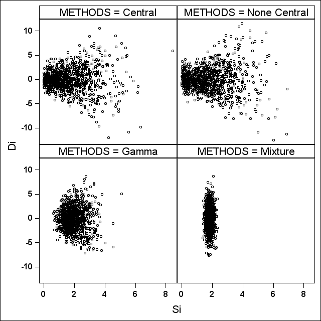
(a) $\tau_{2}^{2}=0$ and $\rho=0$

(b) $\tau_{2}^{2}=\log(2)$ and $\rho=0$

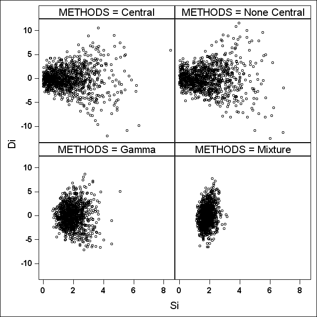
(c) $\tau_{2}^{2}=\log(2)$ and $\rho=0.7$

(d) $\tau_{2}^{2}=\log(2)$ and $\rho=-0.7$

Figure 1: A scatter plot of $S_{i}$ against $D_{i}$ for four different simulation settings (i.e., Central chi-square, Gamma, None-central chi-square, and Mixture of chi-square) based on 100000 simulated studies.

4.1 Simulation Settings

We selected two levels for the number of studies in the simulated meta-analysis ($m\in\{10,50\}$), but we chose to fix the parameters for simulating the sample sizes within studies ($\lambda=100$, $a=b=1$, $p=0.5$). This results in an expected number of sample sizes within each study that is equal to $n_{i0}=n_{i1}=50$, but they could vary strongly from study to study due to the overdispersed Poisson distribution and vary within study due to a binomial division of the total sample size $n_{i0}+n_{i1}$. We considered no treatment effect and two positive levels of treatment effect ($\beta_{1}\in\{0,2,5\}$). The residual variances for the two treatment groups were kept fixed at the levels $\sigma_{0}^{2}=100$ and $\sigma_{1}^{2}=64$, respectively. For the variance of treatment heterogeneity we selected three levels $\tau^{2}\in\{0,2,5\}$. The variance for the random heteroscedasticity was selected at two levels, $\tau_{2}^{2}\in\{0,\log(2)\}$, to simulate effect sizes with and without a random heteroscedasticity. Finally, we selected three levels for the correlation coefficient between the heteroscedasticity and heterogeneity $\rho\in\{-0.7,0,0.7\}$. Clearly, when $\tau_{2}^{2}=0$, the correlation coefficient $\rho$ would not play any role in the simulation. Thus we will study $66=18+48$ different simulation settings (see Table 1 for an overview of the simulation settings for one of the choices of $\beta_{1}$). Each setting will simulate 1000 meta-analysis studies.

Table 1: An overview of the simulation settings and their corresponding mean $I^{2}$ estimated from the simulated data for $\beta_{1}=0$.

$m$ $\tau^{2}$ $\tau_{2}^{2}$ $I^{2}$ (5th percentile - 95th percentile) Central Gamma Non-central Mixture $\rho=-0.7$ $\rho=0$ $\rho=0.7$ 10 0 0 11.6 (0-47.6) 11.5 (0-47.4) 11.8 (0-46.8) - 11.0 (0-46.3) - $\log(2)$ 11.6 (0-47.6) 11.5 (0-47.4) 11.8 (0-46.8) - 11.3 (0-48.1) - 2 0 70.4 (10.0-98.2) 36.0 (0-72.6) 71.4 (12.8-98.5) - 31.6 (0-68.4) - $\log(2)$ 64.3 (0-97.5) 32.7 (0-70.6) 65.3 (0-97.9) 41.8 (0-74.9) 31.5 (0-68.4) 25.2 (0-63.5) 5 0 83.8 (51.4-99.3) 57.2 (3.6-84.3) 84.6 (52.2-84.6) - 51.2 (0-78.6) - $\log(2)$ 79.4 (38.0-99.0) 53.0 (0-82.0) 80.2 (39.2-99.1) 64.2 (21.4-85.7) 52.2 (0-80.0) 41.9 (0-74.8) 50 0 0 6.7 (0-26.5) 6.7 (0-26.7) 6.7 (0-26.2) - 7.0 (0-27.4) - $\log(2)$ 6.7 (0-26.5) 6.7 (0-26.7) 6.7 (0-26.2) - 7.3 (0-27.2) - 2 0 93.1 (78.2-99.7) 44.1 (21.4-61.8) 92.7 (77.9-99.7) - 36.0 (11.1-54.6) - $\log(2)$ 90.7 (71.3-99.5) 39.8 (15.5-58.5) 90.4 (71.3-99.6) 49.4 (29.3-64.7) 37.1 (13.5-56.0) 28.1 (0-49.8) 5 0 97.0 (90.2-99.9) 62.8 (47.0-75.6) 96.9 (89.8-99.9) - 59.0 (43.2-70.9) - $\log(2)$ 95.9 (86.6-99.8) 66.8 (52.4-78.5) 95.7 (86.0-99.8) 71.2 (59.7-80.1) 60.0 (45.3-72.6) 49.7 (30.5-65.8)

Relating our simulation settings to the parameters of model (1), we obviously obtain that $\theta\in\{0,2,5\}$ and $\tau^{2}\in\{0,2,5\}$, since they are direct translations of $\beta_{1}$ and $\tau^{2}$ given above. Thus we could draw a normally distributed random variable $U_{i}$ having a mean equal to $\theta$ and a variance equal to $\tau^{2}$ for all the simulation models from literature. Without random heteroscedasticity ($\tau_{2}^{2}=0$), the residual variance in (1) would become equal to $\sigma_{i}^{2}=\sigma_{0}^{2}/n_{i0}+\sigma_{1}^{2}/n_{i1}$. Using the settings $\sigma_{0}^{2}=100$, $\sigma_{1}^{2}=64$, and $n_{i0}=n_{i1}\approx 50$, the variance $\sigma_{i}^{2}$ would become on average equal to approximately $3.28$, but it will vary across studies due to randomness in $n_{i0}$ and $n_{i1}$. Thus when instead we will draw $\sigma_{i}^{2}$ directly from the central chi-square, the non-central chi-square, or the gamma distribution, we need to choose the distributional parameters such that the expected value is close to $3.28$. For the central chi-square distribution we use $\sigma_{i}^{2}=3.28\chi_{1}^{2}$, having a mean of $3.28$ and a standard deviation of $3.28\sqrt{2}$. For the non-central chi-square distribution we use $\sigma_{i}^{2}=3(0.3+Z_{i})^{2}$, with $Z_{i}\sim N(0,1)$. The expected value is then equal to $3(1+0.09)=3.27$ and the standard deviation is $3\sqrt{2(1+0.18)}$. For the gamma distribution we choose the parameter settings $\Gamma(9,5)$ for standard error $S_{i}$, leading to a mean of $9/5\approx\sqrt{3.28}$ and a standard deviation of $3/5$.

In case of random heteroscedasticity ($\tau_{2}^{2}=\log(2)>0$), the residual variance in (6) for the simulation models from literature would just increase on average with a factor $\sqrt{2}=\exp\{0.5\log(2)\}$ compared to the non-random heteroscedasticity setting $(\tau_{2}^{2}=0$). These simulation models do not alter the relation between $D_{i}$ and $S_{i}$ when a random heteroscedasticity is introduced. Thus for a setting with random heteroscedasticity, we should just multiply the random variables from the setting without random heteroscedasticity with the factor $\sqrt{2}$ when we use the simulation models with the chi-square distributions and $\sqrt[4]{2}$ when we use simulation model with the gamma distribution. Thus correlation coefficient $\rho$, which affects the correlation between $D_{i}$ and $S_{i}$ in our simulation model, does not affect any of the simulation models from literature.

4.2 Publication Bias

The performance of the Trim & Fill and PET-PEESE method in literature was investigated with the same data-driven publication bias selection approach. All studies with a significant effect size are never being excluded from the meta-analysis. For the remaining (non-significant) studies, a standard uniform distributed random variable is generated $U(0,1)$ for each study and the study is included in the meta-analysis when the value of the uniform distributed random variable is less than $\pi_{\mathrm{pub}}$.

The level of significance and the parameter $\pi_{\mathrm{pub}}$ are chosen such that the desired publication rate over all studies is approximately 70%. A study is considered significant when the standardized effect size $D_{i}/S_{i}$ satisfies $D_{i}/S_{i}>z_{\alpha}$, with $z_{q}$ the upper $q$^th quantile of the standard normal distribution function. We used this $z$-test because the aggregated data simulation models from literature did not implement degrees of freedom $df_{i}$, ruling out the use of a $t$-test. In this way a comparison of all aggregated data simulation models would be fair. For $\theta=0$ and $\theta=2$ we used as significance level of $\alpha=0.05$, but for $\theta=5$ we used the smaller significance levels of $\alpha=0.0013$ (three sigma), since some settings had more than 70% significant studies. Thus publication bias depends on the relative performance of other studies. We then pragmatically tuned the parameter $\pi_{\mathrm{pub}}$ for the different settings to obtain the target of 70%. Note that $\pi_{\mathrm{pub}}$ would also be different for the different simulation models, due to the differences in generating the variance $S_{i}^{2}$.

5 Results

5.1 DerSimonian and Laird

The results of the four aggregated data simulation models for $m=10$ are provided in Table 2. Here we did not include publication bias, since it is well-known that DerSimonian and Laird’s estimate would be biased Duval2000a ; Stanley2014 . The correlation coefficient $\rho$ for the random heteroscedastic model was set to $\rho=0$ when we studied heteroscedasticity.

Table 2: Comparison of aggregated data simulation models on bias ($\times 10^{-3}$) and coverage probability (in %) for the DerSimonian and Laird random effects estimator of the overall treatment effect ($m=10$; $\theta=2$; $\rho=0$)

$\tau_{2}^{2}$ $\tau^{2}$ Central Non-central Gamma Mixture Bias (MCSE) 95% CI Bias (MCSE) 95% CI Bias (MCSE) 95% CI Bias (MCSE) 95% CI 0 0 8.5 (06.6) 94.1 11.1 (06.9) 94.6 26.3 (16.5) 94.6 4.5 (18.3) 94.6 2 -7.0 (19.5) 89.6 22.8 (19.7) 90.7 12.7 (22.8) 92.4 6.4 (23.1) 94.7 5 -14.9 (27.3) 92.9 15.2 (27.4) 93.1 9.2 (29.1) 94.0 8.7 (28.8) 95.1 $\log(2)$ 0 10.2 (07.9) 94.1 13.3 (08.2) 94.6 28.7 (18.0) 94.6 -6.1 (17.5) 94.4 2 -6.2 (20.7) 89.1 28.7 (20.9) 89.9 14.6 (24.0) 92.2 -7.9 (22.4) 94.6 5 -15.1 (28.4) 91.9 22.2 (28.6) 92.4 10.6 (30.1) 93.7 -11.1 (27.9) 95.0

All simulation models show hardly any bias, but there is a small difference in the coverage probability for the 95% confidence intervals of the pooled effect size. The simulation model with the mixture of chi-square distributed variances shows a nominal coverage probability, while the other simulation models underestimate the coverage probability when there is heterogeneity. In case the number of studies increases, the difference gets smaller, but remains present (data not shown). The heteroscedasticity ($\rho=0$), which just increases the residual variances for the simulation models (since there is no linear correlation between $D_{i}$ and $S_{i}^{2}$), does not seem to affect any of the results a lot.

5.2 Trim & Fill

For the evaluation of the Trim & Fill method, we implemented the publication bias mechanism. For all aggregated data simulation models, the average number of studies that were included was around 70% (and it ranged from 67% to 73%). Table 3 shows the results on estimation bias and coverage probability for the treatment effect of the Trim & Fill approach under homoscedasticity ($\tau_{2}^{2}=0$) for $m=50$ studies. Results for $m=10$ are slightly worse (data not shown).

Table 3: Comparison of aggregated data simulation models on bias ($\times 10^{-3})$ and coverage probability (in %) for the Trim & Fill estimator ($m=50$; $\tau_{2}^{2}=0$).

$\theta$ $\tau^{2}$ Central Non-central Gamma Mixture Bias (MCSE) 95% CI Bias (MCSE) 95% CI Bias (MCSE) 95% CI Bias (MCSE) 95% CI 0 0 6.9 (02.0) 97.6 8.9 (02.2) 96.9 28.7 (10.4) 90.2 89.4 (15.6) 80.2 2 232.8 (13.0) 74.8 178.9 (12.9) 77.6 130.1 (17.6) 83.3 173.8 (18.3) 81.7 5 398.1 (19.6) 70.3 314.9 (19.6) 73.5 258.7 (22.7) 80.3 288.5 (20.8) 83.9 2 0 10.0 (01.4) 99.1 11.2 (01.5) 97.7 192.8 (09.3) 87.5 261.1 (14.2) 79.0 2 261.2 (11.3) 73.4 248.8 (11.2) 76.4 308.3 (16.6) 78.1 355.3 (16.6) 78.5 5 495.3 (17.3) 64.5 473.1 (17.6) 64.0 434.5 (21.7) 75.2 484.5 (19.9) 78.2 5 0 0.8 (01.3) 98.8 1.2 (01.5) 97.7 114.3 (08.8) 90.8 391.9 (13.7) 71.9 2 -3.1 (11.9) 79.7 -20.3 (12.0) 81.5 272.2 (15.4) 77.6 509.9 (17.1) 68.9 5 221.8 (17.8) 76.7 198.1 (17.6) 77.7 524.4 (20.6) 69.3 675.8 (20.7) 65.8

The simulation models show some different results with respect to bias and coverage probability. The simulation models with the central and non-central distribution do not show any real bias when heterogeneity is absent, while the simulation model with the mixture of chi-square distributions shows a small positive bias at treatment effects $\theta=2$ and $\theta=5$ (Trim & Fill does not correct enough). The coverage probability of the central and non-central chi-square are conservative, but they are underestimated with the gamma and the mixture of chi-square distributions. In the presence of heterogeneity, all simulation models show real biases that increases with the size of heterogeneity. For the central and non-central chi-square distribution, the absolute bias is highest for treatment effect $\theta=2$, but for the mixture of chi-square distributions the bias is highest at treatment effect $\theta=5$. For the gamma distribution, the absolute bias is higher at $\theta=2$ than at $\theta=5$ when heterogeneity is limited, but smaller when heterogeneity is at the level of $\tau^{2}=5$. The mixture of chi-square distributions generally provides the highest bias with respect to the other simulation models.

Random heteroscedasticity with $\rho=0$ does not alter the results observed in Table 3, since it merely increases the residual variance for the simulation models. However, when we select $\rho=-0.7$ or $\rho=0.7$, the correlation between heterogeneity and heteroscedasticity seems to change the results for our aggregated data simulation model (see Table 4). A negative correlation increases the bias and lowers the coverage, while a positive correlation eliminates the bias or changes it to a negative bias, but always with highly liberal coverage probabilities. A negative correlation $\rho=-0.7$ introduces a negative correlation between $D_{i}$ and $S_{i}$ and diminishes the positive correlation between $D_{i}$ and $S_{i}$ that was induced by the publication bias mechanism, masking an asymmetry in the funnel plot that was introduced by the publication bias. A positive correlation $\rho=0.7$ enhances the publication bias, making the Trim & Fill approach correct stronger. For $\theta=0$ the positive bias in Table 3 under homoscedasticity (or under $\rho=0$) is turned into a negative bias, while the observed positive bias for $\theta\in\{2,5\}$ in Table 3 is almost eliminated (Table 4).

Table 4: Bias ($\times 10^{-3})$ and coverage probability (in %) for the Trim & Fill estimator under the mixture of chi-square distributions with heteroscedasticity ($m=50$).

$\theta$	$\tau^{2}$	$\rho=-0.7$		$\rho=0$		$\rho=0.7$
		Bias (MCSE)	95% CI	Bias (MCSE)	95% CI	Bias (MCSE)	95% CI
0	2	609.7 (19.9)	69.0	172.4 (18.6)	81.5	-319.3 (17.7)	74.7
	5	796.6 (24.4)	70.9	285.9 (21.3)	82.5	-344.9 (20.9)	77.9
2	2	755.0 (18.4)	57.5	334.4 (17.0)	78.7	-121.3 (16.2)	85.8
	5	942.0 (22.7)	60.0	457.9 (20.2)	77.9	-123.7 (19.0)	87.3
5	2	873.9 (17.9)	46.3	437.7 (16.5)	70.1	5.7 (14.9)	87.3
	5	1126.6 (22.8)	48.0	587.1 (20.2)	67.6	18.3 (18.0)	86.9

5.3 PET-PEESE

For the evaluation of the PET-PEESE estimator, we also implemented the publication bias mechanism. Since we used the same data as for the Trim & Fill approach, the average number of studies that were included was around 70% (and it ranged from 67% to 73%). Table 5 shows the results on estimation bias and coverage probability for the treatment effect of the PET-PEESE under homoscedasticity ($\tau_{2}^{2}=0$) for $m=50$ studies. Results for $m=10$ are less severe for the simulation models with the central and non-central chi-square distribution when the treatment effect is restricted ($\theta\in\{0,2\}$), but in all other cases the results are more extreme for $m=10$ than for $m=50$.

Table 5: Comparison of aggregated data simulation models on bias ($\times 10^{-3})$ and coverage probability (in %) for the PET-PEESE estimator ($m=50$; $\tau_{2}^{2}=0$).

$\theta$ $\tau^{2}$ Central Non-central Gamma Mixture Bias (MCSE) 95% CI Bias (MCSE) 95% CI Bias (MCSE) 95% CI Bias (MCSE) 95% CI 0 0 1.2 (02.0) 98.1 1.9 (02.2) 97.1 -20.9 (23.4) 97.2 106.3 (102.7) 95.7 2 212.3 (33.0) 26.8 241.2 (31.4) 26.7 78.7 (35.8) 91.0 192.2 (129.6) 95.6 5 352.6 (51.6) 25.7 400.4 (49.6) 25.9 208.6 (48.9) 88.3 337.5 (162.0) 95.6 2 0 2.2 (01.1) 97.7 2.5 (01.3) 95.4 14.0 (19.2) 93.7 129.4 (097.9) 94.9 2 130.7 (31.2) 26.3 157.6 (29.6) 26.4 39.5 (32.1) 86.1 199.6 (124.9) 94.5 5 382.1 (48.5) 24.6 423.4 (46.5) 23.5 127.2 (44.8) 81.1 273.8 (156.1) 94.5 5 0 -5.0 (01.1) 96.2 -5.4 (01.4) 94.3 -41.5 (12.5) 94.6 -281.5 (088.1) 94.7 2 -25.4 (33.2) 26.8 16.1 (30.4) 28.1 62.1 (24.4) 87.7 -228.2 (111.5) 95.5 5 37.0 (50.9) 27.1 114.1 (46.3) 27.1 177.8 (40.5) 82.4 -113.2 (141.7) 95.0

For the PET-PEESE we see biases for the simulation models with the central and non-central chi-square distributions similar to their biases of the Trim & Fill approach, but the coverage probabilities are much smaller when heterogeneity is present. The central and non-central chi-square simulation models simulate studies with very small standard errors (i.e., mimicking extremely large studies in a meta-analysis). These extreme studies, in combination with an independent heterogeneous study effect, have a strong influence on the estimation of the effect size and its standard error in a single meta-analysis. Since the heterogeneity is independent of the standard error, the bias is less affected when averaged out over many meta-analyses, but the confidence interval of the pooled study effect size from a single meta-analysis will not capture the true parameter. The PET-PEESE does not incorporate the heterogeneity in the weights and therefore underestimate the standard error, but the Trim & Fill does account somewhat for the heterogeneity.

The simulation model with the gamma distribution and the mixture of chi-square distributions seem to show less bias with the PET-PEESE than with the Trim & Fill. The bias with PET-PEESE is limited and acceptable for the simulation model with the gamma distribution, although the coverage probability is liberal when heterogeneity is present. The coverage probability for the simulation model with a mixture of chi-square distributions are very close to nominal, even though a small bias is frequently present. The change from a positive bias for treatment effects $\theta\in\{0,2\}$ to a negative bias when $\theta=5$, is difficult to explain, but could be related to the high number of significant effect sizes. For $\theta=5$, Egger’s part hardly plays a role in estimation of the pooled treatment effect, which is not the case for smaller treatment effects. Also the other simulation models show a decline in the bias when the treatment $\theta$ changes from $\{0,2\}$ to $5$, suggesting it is related to the PET-PEESE approach.

Table 6: Bias ($\times 10^{-3})$ and coverage probability (in %) for the PET-PEESE estimator under the mixture of chi-square distributions with heteroscedasticity ($m=50$).

$\theta$	$\tau^{2}$	$\rho=-0.7$		$\rho=0$		$\rho=0.7$
		Bias (MCSE)	95% CI	Bias (MCSE)	95% CI	Bias (MCSE)	95% CI
0	2	2560.5 (55.4)	76.6	238.3 (66.5)	95.5	-2112.5 (49.3)	78.5
	5	3909.2 (66.4)	66.4	364.0 (83.5)	94.9	-3057.6 (48.8)	64.2
2	2	2140.9 (45.2)	66.9	153.9 (59.7)	93.7	-2487.0 (60.5)	78.0
	5	3292.8 (56.9)	56.2	279.6 (77.9)	93.5	-3674.5 (65.9)	63.4
5	2	1680.8 (46.4)	69.0	-118.8 (56.3)	93.8	-2530.4 (66.0)	76.2
	5	2729.8 (58.7)	58.1	-102.4 (71.0)	93.0	-3905.5 (76.9)	64.1

Similar to the Trim & Fill method, a random heteroscedasticity with $\rho=0$ does not alter the results observed in Table 5 a lot, since it does not change the correlation between $D_{i}$ and $S_{i}^{2}$ compared to the setting with homoscedasticity. However, when $\rho=-0.7$ or $\rho=0.7$, we see a similar pattern as for the Trim & Fill approach, but now the heteroscedasticity has a stronger effect (see Table 6). A negative correlation $\rho=-0.7$ reduces the positive correlation between $D_{i}$ and $S_{i}$ induced by the publication bias mechanism, failing the PET-PEESE to correct for publication bias. A positive correlation $\rho=0.7$ enhances the publication bias and making the PET-PEESE over correct.

6 Summary and Discussion

We discussed four simulation models for generating aggregated data in a meta-analysis study. All four models use the well-known random effects model DerSimonian1986 to generate study effect sizes, but each model used their own distribution function for generating the standard error of the study effect size (a central chi-square, a non-central chi-square, a gamma, and a mixture of chi-square distributions). We showed that the mixture of chi-square distributions would follow naturally from a mixed model for individual participant data (IPD), but the other three distributions could not be formulated directly from such an IPD model. The simulation models with a central chi-square, non-central chi-square, and gamma distribution indirectly created a dependency between the study effect size and its standard error, but without introducing a linear dependency. For the mixture of chi-square distributions, a dependency between the study effect size and its standard error was created through a random heteroscedasticity, in line with research on hierarchical heteroscedastic multi-level models, which gave a zero correlation only when the heteroscedasticity is unrelated to the study heterogeneity. The simulation models with a central and non-central chi-square distribution, simulated studies with very small and relatively large standard errors, mimicking meta-analyses with a large variety of study sizes, while the gamma distribution and the mixture of chi-square distributions typically showed standard errors that belong to a smaller variety in study sizes.

Our simulation study showed that the choice of simulation model affects the conclusion of the applied meta-analysis method. The well-known liberal coverage probabilities of the DerSimonian and Laird method of pooled effect size Veroniki2015 ; Brockwell2001 ; Hardy1996 was observed with the simulation models using the central and non-central chi-square distribution, and to a lesser extent with the gamma distribution and the mixture of chi-square distributions. The simulation model using either the gamma distribution or the mixture of chi-square distributions would then lead to the conclusion that the DerSimonian and Laird method had close-to-nominal coverage probabilities.

All simulation models showed some biases for the PET-PEESE approach when heterogeneity is present and the treatment effects are moderate to none. This influence of heterogeneity on the performance of PET-PEESE is in line with literature Stanley2014 ; Alinaghi2018 . However, they applied a different simulation model, where the regression equations (12) and (13) are directly simulated using uniform and normal distributions. Their biases are therefore somewhat different from ours, but this strengthen our point that performances of meta-analysis methods are sensitive to simulation models. Indeed, in our own simulation study for the PET-PEESE we demonstrated that the simulation model with the gamma distribution showed the smallest bias and provided acceptable biases across all settings. Contrary, the simulation model with the mixture of chi-square distributions gave biases of the pooled effect size even when heterogeneity was not present, which was not seen with the other three simulation models. Finally, PET-PEESE was sensitive to standard errors that belong to a larger variety of study sizes, since it gave very small coverage probabilities for the pooled effect size when the central and non-central chi-square distributions were used with study heterogeneity. The simulated meta-analyses typically contained extremely small standard errors that caused an underestimation of the variance of the pooled effect size. To our knowledge, this sensitivity to study sizes has not been presented in literature before.

For the Trim & Fill approach, the simulation model with the gamma distribution showed larger biases in the pooled treatment effect than for the PET-PEESE approach. This is in line with findings that PET-PEESE seems to outperform the Trim & Fill approach Stanley2014 . However, the simulation models with the central and non-central chi-square distributions did not show any large discrepancies between Trim & Fill and PET-PEESE, arguing that Trim & Fill may not necessarily be worse than PET-PEESE. On the other hand, the simulation models with the mixture of chi-square distributions showed substantial positive biases with the Trim & Fill approach and moderate negative biases with the PET-PEESE approach when the treatment effect is strong, an observation not mentioned earlier. Interestingly though, this simulation model with a mixture of chi-square distributions always showed coverage probabilities very close to nominal for all settings for both the Trim & Fill and the PET-PEESE approach, despite the observed biases, contrary to the other simulation models which showed (very) liberal coverage probabilities when heterogeneity is present. Indirectly, the variability in coverage probabilities also showed that the simulation model affects the mean squared error, since the coverage probability for the PET-PEESE is much smaller than for the Trim & Fill approach when the simulation models with central and non-central chi-square distributions are used with heterogeneous effect sizes. Thus mean squared errors are not just affected by publication bias methods Stanley2014 , but also by the choice of simulation model.

When we introduce random heteroscedasticity, an element not studied in literature before, the Trim & Fill and PET-PEESE approach may fail completely in their estimation of the pooled treatment effect. This effect could only be observed with our simulation model, since the simulation models with the central chi-square, non-central chi-square, and the gamma distribution do not have a mechanism to change the joint distribution of the study effect and its standard error. The failure of the publication bias method is not unexpected, since the linear correlation between the study effect and its standard error is influenced by the heteroscedasticity, which is unrelated to publication biases, and confuses the methods for publication bias.

One of the limitations of our study is that we have only considered one study effect (mean difference) for aggregated data meta-analysis that is calculated from one specific heteroscedastic IPD model. Our selected IPD model can also be used to generate binary outcomes by either using a threshold on the continuous response or by using a link function that would change the continuous response into a binary response, leading to several 2x2 contingency tables almalik2018testing . The cell counts can then be used to create an alternative study effect $D_{i}$ (e.g., odds ratio) with its appropriate standard error $S_{i}$, but their (joint) distribution would be currently unknown and may be work for future research. Alternatively, cell counts in 2x2 contingency tables can also be generated differently sidik_comparison_2007 ; berkey_random-effects_1995 ; platt_generalized_1999 ; knapp_improved_2003 using a study-specific effect size at the aggregated level according to the random effects model (5): and with an event probability of the treatment arm based on a logit model. This alternative IPD simulation approach showed that DerSimonian and Laird approach could lead to a biased estimate of the between study variability. Thus the choice of study effect and the different IPD models lead to different ways of simulating aggregated data for studying meta-analysis approaches and consequently could results in a variety of distributions for $(D_{i},S_{i}^{2},df_{i})$ that may deviate from the choices we studied in this paper (see also the discussion of Jackson and White jackson_when_2018 on the hidden distributional assumptions for the aggregated statistics used in meta-analyses). It emphasizes the importance of the choice of simulation model for generating aggregated measures of effect.

Our restricted investigation of simulation models already demonstrated that the choice of simulation model for aggregated data meta-analyses can have an influence on the conclusion of how well a particular meta-analysis approach performs. Most publications in literature do not give any or strong arguments for their choice of simulation models and could therefore implicitly bias their results or conclusions. We recommend the use of multiple simulation models when meta-analysis approaches are being studied to provide a more fair view of the performance of the meta-analysis approach. Otherwise we recommend that researchers provide a strong argument for their choice of simulation model for the aggregated data and show that it would make sense in reality, since not all simulation models we studied had a clear interpretation to statistical models at IPD.

Appendix: Meta-Analysis Methods

In this section we briefly describe the three meta-analysis approaches that we study in our simulation: the DerSimonian and Laird pooled analysis approach and two publication bias adjustment methods: Trim & Fill and PET-PEESE.

DerSimonian and Laird Method

DerSimonian and Laird DerSimonian1986 assumed that the study effect size $D_{i}$ follows model (1) in combination with the normality assumptions on the random effects and with a known variance $\sigma_{i}^{2}$ equal to the observed $S_{i}^{2}$. The pooled estimate for $\theta$ is given by the weighted average $\hat{\theta}_{DSL}=\sum_{i=1}^{m}w_{i}D_{i}/\sum_{i=1}^{m}w_{i}$, with weight $w_{i}$ equal to $w_{i}=[\hat{\tau}^{2}+S_{i}^{2}]^{-1}$ and $\hat{\tau}^{2}$ and estimator of the variance component for the study effect heterogeneity. They proposed the estimator given by

$$\hat{\tau}_{DSL}^{2}=\max\left\{0,\frac{Q-\left(m-1\right)}{\sum_{i=1}^{m}S_{i}^{-2}-\sum_{i=1}^{m}S_{i}^{-4}/\sum_{i=1}^{m}S_{i}^{-2}}\right\},$$

with Cochran’s $Q$-statistic given by $Q=\sum_{i=1}^{m}[S_{i}^{-2}(D_{i}-\bar{D})^{2}]$ and with $\bar{D}$ the weighted average given by $\bar{D}=\sum_{i=1}^{m}[S_{i}^{-2}D_{i}]/\sum_{i=1}^{m}S_{i}^{-2}$. The accompanied standard error $S$ of the pooled estimate $\hat{\theta}_{DSL}$ is given by $S^{2}=1/\sum_{i=1}^{m}w_{i}$. DerSimonian and Laird DerSimonian1986 are not very clear on how to calculate confidence intervals, but based on the work of Cochran Cochran1954 , we assume that the degrees of freedom of $S$ is equal to $m-1$ and use

$$\hat{\theta}_{DSL}\pm t_{\alpha/2,m-1}^{-1}S$$

for the $(1-\alpha)100\%$ confidence interval, with $t_{q,d}^{-1}$ the $(1-q)$ upper quantile of the $t$-distribution with $d$ degrees of freedom. To obtain DerSimonian and Laird’s pooled estimates $\hat{\theta}_{DSL}$ with its 95% confidence limits we applied the R package “meta” Schwarzer2007 .

Trim & Fill Method

The Trim & fill method has been described in detail in Duval and Tweedie Duval2000 ; Duval2000a . In short, studies are first ranked based on their distance from the pooled treatment effect estimated by the random effects model (1), i.e., ranking distances $|D_{i}-\hat{\theta}|$. Next, the number of unobserved studies is estimated using for instance estimator $L_{0}=[4T_{m}-m(m+1)]/[2m-1]$, where $T_{m}$ is the Wilcoxon rank sum test statistic estimated from the ranks of studies with $D_{i}>\hat{\theta}$ (here we assume that $\hat{\theta}$ is positive and it is more likely that studies with effect sizes below $\hat{\theta}$ are potentially missing). We then trim off the $L_{0}$ most extreme studies (i.e., studies with positive effect sizes furthest away from zero) and re-estimate the pooled treatment effect $\hat{\theta}$ without these studies. Then all studies are ranked again, based on their distance to the new pooled estimate, and $L_{0}$ is recomputed. This procedure is repeated until it stabilizes ($L_{0}$ does not change anymore) and we obtain a final estimate $\hat{\theta}$ and a final estimate $L_{0}$ of the number of studies missing. Then we impute $L_{0}$ studies by mirroring the $L_{0}$ studies with the highest effect sizes around the final estimate $\hat{\theta}$ and provide it with the standard error $S_{i}$ from the mirrored study. After imputation, a final pooled estimate with standard error is provided using the random effects model on all $m+L_{0}$ studies. We used the function “trimfill” in the R package “metafor”, with the average treatment effect estimated using the random effects model Viechtbauer2010 .

PET-PEESE Method

The PET-PEESE method is based on the understanding of the bias function in case publication bias is present. Under certain conditions, this bias function can be determined explicitly Stanley2014 , but it is a complicated function of the true effect size and approximations are needed. One approximation is based on Egger test Egger1997 , which investigates the linear relation between the $t$-value $T_{i}=D_{i}/S_{i}$ and the precision $S_{i}^{-1}$, i.e.,

$$T_{i}=\alpha_{0}+\alpha_{1}S_{i}^{-1}+e_{i},$$ (12)

with $\alpha_{0}$ and $\alpha_{1}$ the intercept and slope parameter, respectively, and with residual $e_{i}\sim N\left(0,\nu^{2}\right)$. An intercept deviating from zero ($\alpha_{0}\neq 0$) would indicate publication bias, while the slope in (12) represents the effect size (i.e., $\alpha_{1}=\theta$). However, Stanley and Doucouliagos Stanley2014 demonstrated that the OLS estimator $\hat{\alpha}_{1}$ from (12) would be a biased estimator when it deviates from zero. Thus when null hypothesis $H_{0}:\alpha_{1}=0$ is rejected, they proposed to use the weighted linear regression between study effect $D_{i}$ and variance $S_{i}^{2}$, i.e.,

$$D_{i}=\gamma_{0}+\gamma_{1}S_{i}^{2}+e_{i},$$ (13)

with weights $S_{i}^{-2}$ and report the estimate $\hat{\gamma}_{0}$ as the overall treatment effect $\theta$. This part is called the Precision Effect Estimate with SE (PEESE). In case null hypothesis $H_{0}:\alpha_{1}=0$ is not rejected, the reported estimate is $\hat{\alpha}_{1}$, which is referred to as the Precision Effect Test (PET). Note that model (13) was suggested earlier by Moreno et al. Moreno2011 We used Procedure GLM in SAS to carry out the PET-PEESE method.

We thank the two anonymous reviewers whose comments/suggestions helped improve and clarify this manuscript.

The Authors declare that there is no conflict of interest

The authors ERvdH and OA disclosed receipt of the following financial support for the research, authorship and/or publication of this article: This work was supported by the Netherlands Organization for Scientific Research [grant number 023.005.087]. The author ZZ received no financial support for the research, authorship, and/or publication of this article.

References

- (1) Cochran WG. The combination of estimates from different experiments. Biometrics 1954; 10(1): 101. 10.2307/3001666.
- (2) Bliss C. The statistics of bioassay: With special reference to the vitamins, 1952.
- (3) Borenstein M. Effect sizes for continuous data. In Cooper H, Hedges L and Valentine J (eds.) The handbook of research synthesis and meta-analysis, chapter 12. 2009. pp. 221–235.
- (4) Brockwell SE and Gordon IR. A comparison of statistical methods for meta-analysis. Statistics in Medicine 2001; 20(6): 825–840. 10.1002/sim.650.
- (5) Chung Y, Rabe-Hesketh S and Choi IH. Avoiding zero between-study variance estimates in random-effects meta-analysis. Statistics in Medicine 2013; 32(23): 4071–4089. 10.1002/sim.5821.
- (6) Rukhin AL. Estimating heterogeneity variance in meta-analysis. Journal of the Royal Statistical Society: Series B (Statistical Methodology) 2013; 75(3): 451–469. 10.1111/j.1467-9868.2012.01047.x.
- (7) Ning J, Chen Y and Piao J. Maximum likelihood estimation and EM algorithm of copas-like selection model for publication bias correction. Biostatistics 2017; 18(3): 495–504. 10.1093/biostatistics/kxx004.
- (8) Jackson D and White IR. When should meta-analysis avoid making hidden normality assumptions? Biometrical Journal 2018; 60(6):1040–1058.
- (9) Stanley TD. Meta-regression methods for detecting and estimating empirical effects in the presence of publication selection*. Oxford Bulletin of Economics and Statistics 2008; 70(1): 103–127. 10.1111/j.1468-0084.2007.00487.x.
- (10) Stanley TD and Doucouliagos H. Meta-regression approximations to reduce publication selection bias. Research Synthesis Methods 2014; 5(1): 60–78. 10.1002/jrsm.1095.
- (11) Alinaghi N and Reed WR. Meta-analysis and publication bias: How well does the FAT-PET-PEESE procedure work? Research Synthesis Methods 2018; 9(2): 285–311. 10.1002/jrsm.1298.
- (12) DerSimonian R and Laird N. Meta-analysis in clinical trials. Controlled Clinical Trials 1986; 7(3): 177–188. 10.1016/0197-2456(86)90046-2.
- (13) Duval S and Tweedie R. Trim and fill: A simple funnel-plot-based method of testing and adjusting for publication bias in meta-analysis. Biometrics 2000; 56(2): 455–463. 10.1111/j.0006-341x.2000.00455.x.
- (14) Duval S and Tweedie R. A nonparametric “trim and fill” method of accounting for publication bias in meta-analysis. Journal of the American Statistical Association 2000; 95(449): 89–98. 10.1080/01621459.2000.10473905.
- (15) Dadi AF, Wolde HF, Baraki AG et al. Epidemiology of antenatal depression in africa: a systematic review and meta-analysis. BMC Pregnancy and Childbirth 2020; 20(1). 10.1186/s12884-020-02929-5.
- (16) Liu S and Niu W. Anxiety and depression prevalence in children, adolescents, and young adults with life-limiting conditions. JAMA Pediatrics 2020; 174(2): 208. 10.1001/jamapediatrics.2019.4803.
- (17) Torous J, Lipschitz J, Ng M et al. Dropout rates in clinical trials of smartphone apps for depressive symptoms: A systematic review and meta-analysis. Journal of Affective Disorders 2020; 263: 413–419. 10.1016/j.jad.2019.11.167.
- (18) Molenberghs G and Kenward M. Missing data in clinical studies, volume 61. John Wiley & Sons, 2007.
- (19) Rosenbaum PR. Observational Studies. Springer New York, 2002. 10.1007/978-1-4757-3692-2.
- (20) Davidian M and Carroll RJ. Variance function estimation. Journal of the American Statistical Association 1987; 82(400): 1079–1091. 10.1080/01621459.1987.10478543.
- (21) Quintero A and Lesaffre E. Multilevel covariance regression with correlated random effects in the mean and variance structure. Biometrical Journal 2017; 59(5): 1047–1066. 10.1002/bimj.201600193.
- (22) McGaw B and Glass GV. Choice of the metric for effect size in meta-analysis. American Educational Research Journal 1980; 17(3): 325–337. 10.3102/00028312017003325.
- (23) Satterthwaite FE. An approximate distribution of estimates of variance components. Biometrics Bulletin 1946; 2(6): 110. 10.2307/3002019.
- (24) van den Heuvel ER. A comparison of estimation methods on the coverage probability of satterthwaite confidence intervals for assay precision with unbalanced data. Communications in Statistics - Simulation and Computation 2010; 39(4): 777–794. 10.1080/03610911003646373.
- (25) Hardy RJ and Thompson SG. A likelihood approach to meta-analysis with random effects. Statistics in Medicine 1996; 15(6): 619–629. 10.1002/(SICI)1097-0258(19960330)15:6¡619::AID-SIM188¿3.0.CO;2-A.
- (26) Sidik K and Jonkman JN. A simple confidence interval for meta-analysis. Statistics in Medicine 2002; 21(21): 3153–3159. 10.1002/sim.1262.
- (27) Light RJ and Pillemer DB. Summing up: The Science of Reviewing Research, volume 15. Harvard University Press, 1986. 10.2307/1175260.
- (28) Schwarzer G et al. meta: An r package for meta-analysis. R news 2007; 7(3): 40–45.
- (29) Viechtbauer W. Conducting meta-analyses in R with the metafor Package. Journal of Statistical Software 2010; 36(3). 10.18637/jss.v036.i03.
- (30) Egger M, Smith GD, Schneider M et al. Bias in meta-analysis detected by a simple, graphical test. BMJ 1997; 315(7109): 629–634. 10.1136/bmj.315.7109.629.
- (31) Moreno SG, Sutton AJ, Ades AE et al. Adjusting for publication biases across similar interventions performed well when compared with gold standard data. Journal of Clinical Epidemiology 2011; 64(11): 1230–1241. 10.1016/j.jclinepi.2011.01.009.
- (32) Veroniki AA, Jackson D, Viechtbauer W et al. Methods to estimate the between-study variance and its uncertainty in meta-analysis. Research Synthesis Methods 2015; 7(1): 55–79. 10.1002/jrsm.1164.
- (33) Sidik K and Jonkman JN. A comparison of heterogeneity variance estimators in combining results of studies. Statistics in Medicine 2007; 26(9): 1964–1981.
- (34) Berkey CS, Hoaglin DC, Mosteller F et al. A random-effects regression model for meta-analysis. Statistics in Medicine 1995; 14(4): 395–411.
- (35) Platt RW, Leroux BG, and Breslow N. Generalized linear mixed models for meta-analysis. Statistics in Medicine 1999; 18(6): 643–654.
- (36) Knapp G and Hartung J. Improved tests for a random effects meta-regression with a single covariate. Statistics in Medicine 2003; 22(17): 2693–2710.
- (37) Almalik O and van den Heuvel ER. Testing homogeneity of effect sizes in pooling 2x2 contingency tables from multiple studies: a comparison of methods. Cogent Mathematics & Statistics 2018; 5(1): 1478698.