Higher-rank discrete symmetries in the IBM.
III Tetrahedral shapes

Abstract

In the context of the $sf$-IBM, the interacting boson model with $s$ and $f$ bosons, the conditions are derived for a rotationally invariant and parity-conserving Hamiltonian with up to two-body interactions to have a minimum with tetrahedral shape in its classical limit. A degenerate minimum that includes a shape with tetrahedral symmetry can be obtained in the classical limit of a Hamiltonian that is transitional between the two limits of the model, ${\rm U}_{f}(7)$ and ${\rm SO}_{sf}(8)$. The conditions for the existence of such a minimum are derived. The system can be driven towards an isolated minimum with tetrahedral shape through a modification of two-body interactions between the $f$ bosons. General comments are made on the observational consequences of the occurrence of shapes with a higher-rank discrete symmetry in the context of algebraic models.

, and

1 Introduction

This paper is a continuation of Refs. [1, 2], henceforth referred to as I and II, as part of a series concerning nuclear shapes with a higher-rank discrete symmetry in the framework of the interacting boson model (IBM) and its possible extensions [3]. In I and II we considered the case of hexadecapole deformation giving rise to shapes with octahedral symmetry and their manifestation in the $sdg$-IBM. In the present paper we turn our attention to tetrahedral symmetry.

Shapes with tetrahedral discrete symmetry occur in lowest order through a particular kind of octupole deformation, namely $Y_{3\mu}(\theta,\phi)$ with $\mu=\pm 2$, and all other deformations equal to zero [4, 5, 6]. Whereas evidence for hexadecapole deformation in nuclei is circumstantial at best, such is not the case for the octupole degree of freedom. Octupole excitations in spherical nuclei are well documented (see, e.g., the review [7]) and there is even experimental evidence for nuclei with a permanent octupole deformation [8]. This makes the search for nuclear shapes with tetrahedral symmetry all the more compelling.

The algebraic description of the octupole degree of freedom requires the introduction of an $f$ boson with angular momentum $\ell=3$ and negative parity, as was already suggested in the early papers on the IBM [9, 10, 11]. In principle, the $f$ boson should be considered in addition to the bosons of the elementary version of the model since for a realistic description of nuclear collective behavior the quadrupole degree of freedom, and therefore the $d$ boson, cannot be neglected. Furthermore, an octupole deformation causes a shift in the center of mass that must be balanced by a dipole deformation, which necessitates the introduction of a $p$ boson [12]. One concludes therefore that the search for tetrahedral deformation should be carried out in the framework of the $spdf$-IBM, the properties of which have been studied in detail in Refs. [13, 14, 15]. Unfortunately, a catastrophe analysis of this model is a rather complicated problem and the following simplification suggests itself based on our experience with the search for octahedral deformation in the context of the $sdg$-IBM. Because quadrupole deformations must vanish for the nucleus to acquire a shape with a higher-rank discrete symmetry, it transpires that the $d$ boson is not an essential ingredient in our search, the reason being that it should not or only weakly couple to the other bosons. In fact, the most important conditions for the realization of a shape with octahedral symmetry, as obtained in the $sdg$-IBM in I and II, could just as well have been derived in the context of the $sg$-IBM. By analogy, we suggest therefore that a search for tetrahedral deformation in an algebraic context can be carried out in the simpler $sf$-IBM, which is the subject matter of the present paper. It should be recognized however that the absence of a rotational SU(3) limit in the $sf$-IBM constitutes a limitation of the present approach.

The paper is structured as follows. In Section 2 we recall the parameterization of octupole shapes and how, within this parameterization, a shape with tetrahedral symmetry can be realized. Section 3 introduces the rotationally invariant, parity-conserving Hamiltonian of the $sf$-IBM with up to two-body interactions, of which the dynamical symmetries are discussed in Section 4 and the classical limit in Section 5. The main results of this paper are presented in Section 6, where a catastrophe analysis of the classical energy surface is carried out to unveil the existence of minima at shapes with tetrahedral symmetry. Finally, in Section 7 the conclusions of this work are summarized.

2 Octupole and tetrahedral shapes

In case of a pure octupole deformation seven variables $\alpha_{3\mu}$ are needed to define the intrinsic shape as well as the orientation of that shape in the laboratory frame. One is therefore confronted with the problem of the separation of intrinsic from orientation variables. While this problem has a natural solution in the case of quadrupole deformation [16, 17, 18], namely intrinsic axes that are defined by the mutually perpendicular symmetry planes of the quadrupole shape, no such solution presents itself in the case of octupole deformation [19]. The parameterization of Hamamoto et al. [20] is used in the following and the surface is written as

$$R_{\rm o}(\theta,\phi) = R_{0}\Biggl{[}1+a_{30}Y_{30}(\theta,\phi)$$ (1)

$$\qquad\;+\sum_{\mu=1}^{3}a_{3\mu}Y_{3\mu}^{\pi_{\mu}}(\theta,\phi)-\imath\sum_{\mu=1}^{3}b_{3\mu}Y_{3\mu}^{-\pi_{\mu}}(\theta,\phi)\Biggr{]},$$

with $\pi_{\mu}\equiv(-)^{\mu}$ and where the combinations

$$Y_{\lambda\mu}^{\pm}(\theta,\phi)=\frac{1}{\sqrt{2}}\left[Y_{\lambda\mu}(\theta,\phi)\pm Y_{\lambda-\mu}(\theta,\phi)\right],$$ (2)

are introduced in terms of the usual spherical harmonics $Y_{\lambda\mu}(\theta,\phi)$. The surface $R_{\rm o}(\theta,\phi)$ is determined by the seven (real) variables $\{a_{30},a_{3\mu},b_{3\mu},\mu=1,2,3\}$. Hamamoto et al. [20] define the intrinsic shape through the four variables $\{\beta_{3},\delta_{3},\vartheta_{3},\varphi_{3}\}$

$$b_{32} = \beta_{3}\sin\delta_{3},$$

$$a_{30} = \beta_{3}\cos\delta_{3}\sin\vartheta_{3}\cos\varphi_{3},$$

$$\sqrt{\textstyle{\frac{3}{8}}}a_{31}-\sqrt{\textstyle{\frac{5}{8}}}a_{33} = \beta_{3}\cos\delta_{3}\sin\vartheta_{3}\sin\varphi_{3},$$

$$\sqrt{\textstyle{\frac{3}{8}}}b_{31}+\sqrt{\textstyle{\frac{5}{8}}}b_{33} = \beta_{3}\cos\delta_{3}\cos\vartheta_{3},$$ (3)

while three combinations are set to zero,

$$a_{32}=\sqrt{\textstyle{\frac{5}{8}}}a_{31}+\sqrt{\textstyle{\frac{3}{8}}}a_{33}=-\sqrt{\textstyle{\frac{5}{8}}}b_{31}+\sqrt{\textstyle{\frac{3}{8}}}b_{33}=0.$$ (4)

All possible intrinsic octupole-deformed shapes are covered by the following three ranges of parameters:

$${\rm(a)} \beta_{3}>0,\quad-\textstyle{\frac{1}{2}}\pi<\delta_{3}<\textstyle{\frac{1}{2}}\pi,\quad\tan^{-1}\sqrt{2}\leq\vartheta_{3}<\textstyle{\frac{1}{2}}\pi,\quad 0<\varphi_{3}\leq\textstyle{\frac{1}{4}}\pi,$$

$${\rm(b)} \beta_{3}>0,\quad{\rm if}\quad\delta_{3}=\textstyle{\frac{1}{2}}\pi,$$

$${\rm(c)} \beta_{3}>0,\quad 0\leq\delta_{3}<\textstyle{\frac{1}{2}}\pi,\quad 0\leq\varphi_{3}\leq\textstyle{\frac{1}{4}}\pi,\quad{\rm if}\quad\vartheta_{3}=\textstyle{\frac{1}{2}}\pi,$$ (5)

where for range (a) the additional constraint $(\tan\vartheta_{3})(\sin\varphi_{3})\geq 1$ should be satisfied. The parameterization (5) has the important property that a given intrinsic shape occurs only once over the entire range.

A shape with tetrahedral symmetry implies a vanishing quadrupole deformation, $\beta_{2}=0$, and can be realized in lowest order with an octupole deformation with $\mu=\pm 2$ [21, 22]. For the octupole parameterization (3) this implies $\beta_{3}>0$ and $\delta_{3}={\frac{1}{2}}\pi$, in which case the nuclear surface (1) reduces to

$$\frac{R_{\rm o}(\theta,\phi)}{R_{0}}=1+\imath\beta_{3}Y_{32}^{-}(\theta,\phi)=1-\sqrt{\frac{105}{16\pi}}\beta_{3}(\sin\theta)^{2}\cos\theta\sin 2\phi.$$ (6)

A single parameter, $\beta_{3}$, defines the surface with tetrahedral symmetry.

3 The $sf$ interacting boson model

In this section the most general rotationally invariant and parity-conserving $sf$-IBM Hamiltonian with up to two-body interactions is presented. It has the same formal expression as given in I with the additional constraint that parity is conserved.

A Hamiltonian of the $sf$-IBM conserves the total number of bosons and can therefore be written in terms of the $(1+7)^{2}=64$ operators $b_{\ell m}^{\dagger}b_{\ell^{\prime}m^{\prime}}$, where $b_{\ell m}^{\dagger}$ ($b_{\ell m}$) creates (annihilates) a boson with angular momentum $\ell$ and $z$ projection $m$. A boson-number-conserving Hamiltonian with up to two-body interactions is of the form

$$\hat{H}=\hat{H}_{1}+\hat{H}_{2},$$ (7)

with a one-body term

$$\hat{H}_{1} = \epsilon_{s}[s^{\dagger}\times\tilde{s}]^{(0)}-\epsilon_{f}\sqrt{7}[f^{\dagger}\times\tilde{f}]^{(0)}$$ (8)

$$= \epsilon_{s}\,s^{\dagger}\cdot\tilde{s}+\epsilon_{f}\,f^{\dagger}\cdot\tilde{f}=\epsilon_{s}\hat{n}_{s}+\epsilon_{f}\hat{n}_{f},$$

and a two-body interaction

$$\hat{H}_{2}=\sum_{\ell_{1}\leq\ell_{2},\ell^{\prime}_{1}\leq\ell^{\prime}_{2},L}\frac{(-)^{L}v^{L}_{\ell_{1}\ell_{2}\ell^{\prime}_{1}\ell^{\prime}_{2}}}{\sqrt{(1+\delta_{\ell_{1}\ell_{2}})(1+\delta_{\ell^{\prime}_{1}\ell^{\prime}_{2}})}}[b^{\dagger}_{\ell_{1}}\times b^{\dagger}_{\ell_{2}}]^{(L)}\cdot[\tilde{b}_{\ell^{\prime}_{2}}\times\tilde{b}_{\ell^{\prime}_{1}}]^{(L)},$$ (9)

with $\tilde{b}_{\ell m}\equiv(-)^{\ell-m}b_{\ell,-m}$. The multiplication $\times$ refers to coupling in angular momentum (shown as an upper-index in round brackets), the dot $\cdot$ indicates a scalar product, $b^{\dagger}_{\ell}\cdot\tilde{b}_{\ell}\equiv\sum_{m}b^{\dagger}_{\ell m}b_{\ell m}$, $\hat{n}_{\ell}$ is the number operator for the $\ell$ boson and the coefficient $\epsilon_{\ell}$ is its energy. The coefficients $v^{L}_{\ell_{1}\ell_{2}\ell^{\prime}_{1}\ell^{\prime}_{2}}$ are the interaction matrix elements between normalized two-boson states, $v^{L}_{\ell_{1}\ell_{2}\ell^{\prime}_{1}\ell^{\prime}_{2}}\equiv\langle\ell_{1}\ell_{2};LM_{L}|\hat{H}_{2}|\ell^{\prime}_{1}\ell^{\prime}_{2};LM_{L}\rangle$. Conservation of parity implies that this interaction matrix element vanishes unless $(-)^{\ell_{1}+\ell_{2}}=(-)^{\ell^{\prime}_{1}+\ell^{\prime}_{2}}$. Also, it will be assumed in the following that all Hamiltonians are Hermitian so that $v^{L}_{\ell_{1}\ell_{2}\ell^{\prime}_{1}\ell^{\prime}_{2}}=v^{L}_{\ell^{\prime}_{1}\ell^{\prime}_{2}\ell_{1}\ell_{2}}$.

4 Dynamical symmetries of the $sf$-IBM

Although the $sf$-IBM is a schematic model, it of some interest to study its dynamical symmetries since these correspond to two possible, basic manifestations of octupole collectivity in nuclei.

The 64 operators $b_{\ell m}^{\dagger}b_{\ell^{\prime}m^{\prime}}$ with $\ell,\ell^{\prime}=0,3$ generate the Lie algebra U(8) whose substructure therefore determines the dynamical symmetries of the $sf$-IBM. The first limit is obtained by eliminating from the generators of U(8) those that involve the $s$ boson; it is specified by the following chain of nested algebras:

$$({\rm I})\qquad\begin{array}[]{ccccccc}{\rm U}_{sf}(8)&\supset&{\rm U}_{f}(7)&\supset&{\rm SO}_{f}(7)&\supset&{\rm SO}_{f}(3)\\ \downarrow&&\downarrow&&\downarrow&&\downarrow\\[0.0pt] [N]&&n_{f}&&\upsilon_{f}&\nu_{f}&L\end{array},$$ (10)

where the subscripts ‘$s$’ and/or ‘$f$’ are a reminder of the bosons that make up the generators of the algebra (see below). Below each algebra the associated quantum number is given: $N$ is the total number of bosons, $n_{f}$ is the number of $f$ bosons, $\upsilon_{f}$ is the $f$-boson seniority (i.e., the number of $f$ bosons not in pairs coupled to angular momentum zero) and $L$ is the angular momentum generated by the $f$ bosons. (Since $L$ coincides with the total angular momentum, its subscript ‘$f$’ is suppressed.) Additional multiplicity labels, collectively denoted as $\nu_{f}$ and not associated to an algebra, are needed between ${\rm SO}_{f}(7)$ and ${\rm SO}_{f}(3)$. In this limit, which shall be referred to as ${\rm U}_{f}(7)$ or limit I, the separate numbers of $s$ and $f$ bosons are conserved, giving rise to a vibrational-like spectrum with a spherical shape of the ground state and oscillations in the octupole degree of freedom.

The second dynamical symmetry corresponds to the following chain of nested algebras:

$$({\rm II})\qquad\begin{array}[]{ccccccc}{\rm U}_{sf}(8)&\supset&{\rm SO}_{sf}(8)&\supset&{\rm SO}_{f}(7)&\supset&{\rm SO}_{f}(3)\\ \downarrow&&\downarrow&&\downarrow&&\downarrow\\[0.0pt] [N]&&\upsilon_{sf}&&\upsilon_{f}&\nu_{f}&L\end{array}.$$ (11)

The algebras and quantum numbers are identical to those in the vibrational limit (10) but for the appearance of ${\rm SO}_{sf}(8)$ and its associated label $\upsilon_{sf}$, resulting from the pairing of $s$ and $f$ bosons. As shown in Section 5, the ground state acquires a permanent octupole deformation in this limit, which shall be referred to as ${\rm SO}_{sf}(8)$ or limit II.

The dynamical symmetries of ${\rm U}_{sf}(8)$ describe the two basic manifestations of octupole collectivity in nuclei: octupole vibrations around a spherical shape (limit I) or a permanent octupole deformation (limit II). The latter limit is of relevance in the search for tetrahedral deformation but it has the unrealistic feature that the energies of the $s$ and $f$ boson are taken to be degenerate. In Sections 5 and 6 we investigate to what extent non-degenerate single-boson energies can be accommodated while still preserving an octupole-deformed minimum, and whether that minimum can have tetrahedral symmetry.

For further reference, we list some of the properties of limits I and II. The classification of limits I and II can be summarized with the algebraic lattice

$$\begin{array}[]{c}{\rm U}_{sf}(8)\\ \swarrow\quad\searrow\\ \quad{\rm U}_{f}(7)\quad{\rm SO}_{sf}(8)\\ \searrow\quad\swarrow\\ {\rm SO}_{f}(7)\\ \downarrow\\ {\rm SO}_{f}(3)\end{array}.$$ (12)

The generators of the different subalgebras in the lattice (12) are

$${\rm U}_{f}(7) :\quad \{[f^{\dagger}\times\tilde{f}]^{(\lambda)}_{\mu},\lambda=0,\dots,6\},$$

$${\rm SO}_{sf}(8) :\quad \{[s^{\dagger}\times\tilde{f}-f^{\dagger}\times\tilde{s}]^{(3)}_{\mu},[f^{\dagger}\times\tilde{f}]^{(\lambda)}_{\mu},\lambda=1,3,5\},$$

$${\rm SO}_{f}(7) :\quad \{[f^{\dagger}\times\tilde{f}]^{(\lambda)}_{\mu},\lambda=1,3,5\},$$

$${\rm G}_{2} :\quad \{[f^{\dagger}\times\tilde{f}]^{(\lambda)}_{\mu},\lambda=1,5\},$$

$${\rm SO}_{f}(3) :\quad \{\hat{L}_{\mu}\equiv\sqrt{28}[f^{\dagger}\times\tilde{f}]^{(1)}_{\mu}\}.$$ (13)

Note the presence of the additional (exceptional) algebra ${\rm G}_{2}$, which occurs in between ${\rm SO}_{f}(7)$ and ${\rm SO}_{f}(3)$ [23]. It does not appear in Eqs. (10) and (11) because in symmetric irreducible representations the quadratic Casimir operators of ${\rm SO}_{f}(7)$ and ${\rm G}_{2}$ have identical expectation values. The exceptional algebra ${\rm G}_{2}$ is therefore discarded from the classifications (10), (11) and (12) without loss of generality.

The explicit expressions of linear and quadratic Casimir operators of the algebras appearing in the lattice (12) are

$$\hat{C}_{1}[{\rm U}_{sf}(8)] = \hat{N}=\hat{n}_{s}+\hat{n}_{f},$$

$$\hat{C}_{2}[{\rm U}_{sf}(8)] = \hat{N}(\hat{N}+7),$$

$$\hat{C}_{1}[{\rm U}_{f}(7)] = \hat{n}_{f},$$

$$\hat{C}_{2}[{\rm U}_{f}(7)] = \hat{n}_{f}(\hat{n}_{f}+6),$$

$$\hat{C}_{2}[{\rm SO}_{sf}(8)] = [s^{\dagger}\times\tilde{f}-f^{\dagger}\times\tilde{s}]^{(3)}\cdot[s^{\dagger}\times\tilde{f}-f^{\dagger}\times\tilde{s}]^{(3)}+\hat{C}_{2}[{\rm SO}_{f}(7)],$$

$$\hat{C}_{2}[{\rm SO}_{f}(7)] = 2\sum_{\lambda\;{\rm odd}}[f^{\dagger}\times\tilde{f}]^{(\lambda)}\cdot[f^{\dagger}\times\tilde{f}]^{(\lambda)},$$

$$\hat{C}_{2}[{\rm SO}_{f}(3)] = \hat{L}\cdot\hat{L}.$$ (14)

The expressions for the quadratic Casimir operators $\hat{C}_{2}[{\rm U}_{sf}(8)]$ and $\hat{C}_{2}[{\rm U}_{f}(7)]$ are not general but are valid in symmetric irreducible representations of ${\rm U}_{sf}(8)$ and ${\rm U}_{f}(7)$. A rotationally invariant and parity-conserving Hamiltonian with up to two-body interactions can be written in terms of the Casimir operators (14),

$$\hat{H}_{\rm sym} = \epsilon_{s}\,\hat{n}_{s}+\epsilon_{f}\,\hat{n}_{f}+a_{f}\,\hat{C}_{2}[{\rm U}_{f}(7)]+b_{sf}\,\hat{P}_{sf}^{\dagger}\hat{P}_{sf}+b_{f}\,\hat{C}_{2}[{\rm SO}_{f}(7)]$$ (15)

$$+c_{f}\,\hat{C}_{2}[{\rm SO}_{f}(3)],$$

where $\epsilon_{\ell}$, $a_{\ell}$, $b_{\ell}$, $b_{\ell\ell^{\prime}}$ and $c_{\ell}$ are parameters. The quadratic Casimir operator of ${\rm U}_{sf}(8)$ is omitted for simplicity since it gives a constant contribution for a fixed boson number $N=n_{s}+n_{f}$. The pairing interaction for $s$ and $f$ bosons can be expressed in terms of Casimir operators,

$$\hat{P}^{\dagger}_{sf}\hat{P}_{sf}=\hat{C}_{2}[{\rm U}_{sf}(8)]-\hat{C}_{1}[{\rm U}_{sf}(8)]-\hat{C}_{2}[{\rm SO}_{sf}(8)],$$ (16)

where $\hat{P}^{\dagger}_{sf}\equiv s^{\dagger}s^{\dagger}-f^{\dagger}\cdot f^{\dagger}$. Equation (15) is the most general Hamiltonian with up to two-body interactions that can be written in terms of invariant operators of the lattice (12). It is intermediate between the limits I and II but has less parameters than the general Hamiltonian (7). The latter contains seven boson–boson interaction matrix elements whereas the symmetry Hamiltonian (15) has only four two-body parameters.

The ${\rm U}_{f}(7)$ limit is attained for $b_{sf}=0$ leading to the eigenvalues

$$E_{\rm I}=\epsilon_{s}\,n_{s}+\epsilon_{f}\,n_{f}+a_{f}\,n_{f}(n_{f}+6)+b_{f}\,\upsilon_{f}(\upsilon_{f}+5)+c_{f}\,L(L+1).$$ (17)

The ${\rm SO}_{sf}(8)$ limit occurs for $\epsilon_{s}=\epsilon_{f}\equiv\epsilon_{sf}$ and $a_{f}=0$, in which case the Hamiltonian’s eigenstates have the eigenvalues

$$E_{\rm II} = \epsilon_{sf}\,N+b_{sf}[N(N+6)-\upsilon_{sf}(\upsilon_{sf}+6)]+b_{f}\,\upsilon_{f}(\upsilon_{f}+5)$$ (18)

$$+c_{f}\,L(L+1).$$

The eigenspectra in two limits are then determined with the help of the branching rules

$${\rm U}_{sf}(8)\supset{\rm U}_{f}(7) \quad:\quad [N]\mapsto n_{f}=0,1,\dots,N,$$

$${\rm U}_{f}(7)\supset{\rm SO}_{f}(7) \quad:\quad n_{f}\mapsto\upsilon_{f}=n_{f},n_{f}-2,\dots,1\;{\rm or}\;0,$$

$${\rm U}_{sf}(8)\supset{\rm SO}_{sf}(8) \quad:\quad [N]\mapsto\upsilon_{sf}=N,N-2,\dots,1\;{\rm or}\;0,$$

$${\rm SO}_{sf}(8)\supset{\rm SO}_{f}(7) \quad:\quad \upsilon_{sf}\mapsto\upsilon_{f}=0,1,\dots,\upsilon_{sf}.$$

The ${\rm SO}_{f}(7)\supset{\rm SO}_{f}(3)$ reduction from seniority to angular momentum is more complicated due to the multiplicity problem. A closed formula is available for the number of times the angular momentum $L$ occurs for a given seniority $\upsilon_{f}$ in terms of an integral over characters of the orthogonal algebras SO(7) and SO(3) [24]. This number $d(\upsilon_{f},L)$ is given by complex integral [25]

$$d(\upsilon_{f},L)=\frac{i}{2\pi}\oint_{|z|=1}\frac{(z^{2L+1}-1)(z^{2\upsilon_{f}+5}-1)\prod_{k=1}^{4}(z^{\upsilon_{f}+k}-1)}{z^{3\upsilon_{f}+L+2}\prod_{k=1}^{4}(z^{k+1}-1)}dz,$$ (20)

which, due to Cauchy’s theorem, can be evaluated by taking the negative of the residue of its integrand. An alternative recursive method to determine the ${\rm SO}_{f}(7)\supset{\rm SO}_{f}(3)$ reduction was proposed by Rohoziński [26]. Tables of multiplicities $d(\upsilon_{f},L)$ can be found in Refs. [26, 27].

Figure 1: Energy spectra in the ${\rm U}_{f}(7)$ and ${\rm SO}_{sf}(8)$ limits of the $sf$-IBM for $N=6$ bosons. For the ${\rm U}_{f}(7)$ spectrum the non-zero parameters in the Hamiltonian (15) are $\epsilon_{f}-\epsilon_{s}=1000$, $b_{f}=25$ and $c_{f}=10$ keV. For the ${\rm SO}_{sf}(8)$ spectrum the non-zero parameters are $\epsilon_{f}-\epsilon_{s}=0$, $b_{sf}=100$, $b_{f}=75$ and $c_{f}=10$ keV.

Typical energy spectra in the ${\rm U}_{f}(7)$ and ${\rm SO}_{sf}(8)$ limits are shown in Fig. 1. The ${\rm U}_{f}(7)$ spectrum displays octupole-phonon multiplets characterized by a fixed number of $f$ bosons, $n_{f}=0,1,\dots$ The multiplets are further structured by the seniority quantum number: the $n_{f}=2$ multiplet has $\upsilon_{f}=2$ except for the $0^{+}$ level, which has $\upsilon_{f}=0$, the $n_{f}=3$ multiplet has $\upsilon_{f}=3$ except for the $3^{-}$ level, which has $\upsilon_{f}=1$, etc. The ${\rm SO}_{sf}(8)$ spectrum contains sets of levels with $\upsilon_{sf}=N,N-2,\dots$ and, due the repulsive $sf$-pairing, $\upsilon_{sf}=N$ levels are lowest in energy. Multiplets characterized by a seniority quantum number $\upsilon_{f}=0,1,\dots$ occur within each ${\rm SO}_{sf}(8)$ multiplet.

5 Classical limit of the $sf$-IBM

The classical limit of an arbitrary interacting boson Hamiltonian is its expectation value in a coherent state [28], which is a function of the deformation variables and is to be interpreted as a total-energy surface. The method was first proposed for the $sd$-IBM [29, 30]. The coherent state for the $sf$-IBM is inspired by the surface (1),

$$|N;a_{3\mu},b_{3\mu}\rangle\propto\Gamma(a_{3\mu},b_{3\mu})^{N}|{\rm o}\rangle,$$ (21)

with [31]

$$\Gamma(a_{3\mu},b_{3\mu})=s^{\dagger}+a_{30}f^{\dagger}_{0}+\sum_{\mu=1}^{3}a_{3\mu}(f^{\pi_{\mu}}_{\mu})^{\dagger}+\imath\sum_{\mu=1}^{3}b_{3\mu}(f^{-\pi_{\mu}}_{\mu})^{\dagger},$$ (22)

where $|{\rm o}\rangle$ is the boson vacuum and the creation operators are defined as

$$(f^{\pm}_{\mu})^{\dagger}=\frac{1}{\sqrt{2}}\left(f_{\mu}^{\dagger}\pm f_{-\mu}^{\dagger}\right).$$ (23)

The coefficients $a_{3\mu}$ and $b_{3\mu}$ have the interpretation of the shape variables appearing in the expansion (1). In contrast to the geometric model of Bohr and Mottelson [18] where deformation is associated with the entire nucleus, in the IBM it is generated by the valence nucleons only. As a result, the shape variables in both models are proportional but not identical [32]. In the parameterization (3) the radial parameter $\beta_{3}$ in the geometric model and in the IBM are proportional while the angles parameters have an identical interpretation.

The coherent state based on the parameterization (3) reads

$$|N;\beta_{3},\delta_{3},\vartheta_{3},\varphi_{3}\rangle=\sqrt{\frac{1}{N!(1+\beta_{3}^{2})^{N}}}\Gamma(\beta_{3},\delta_{3},\vartheta_{3},\varphi_{3})^{N}|{\rm o}\rangle,$$ (24)

with

$$\Gamma(\beta_{3},\delta_{3},\vartheta_{3},\varphi_{3})$$

$$=s^{\dagger}+\beta_{3}\Bigl{[}\cos\delta_{3}\sin\vartheta_{3}\cos\varphi_{3}f^{\dagger}_{0}+\imath\sqrt{\textstyle{\frac{1}{2}}}\sin\delta_{3}(f^{\dagger}_{-2}-f^{\dagger}_{+2})$$

$$\qquad\quad-\sqrt{\textstyle{\frac{3}{16}}}\cos\delta_{3}\Bigl{(}\sin\vartheta_{3}\sin\varphi_{3}(f^{\dagger}_{-1}-f^{\dagger}_{+1})+\imath\cos\vartheta_{3}(f^{\dagger}_{-1}+f^{\dagger}_{+1})\Bigr{)}$$

$$\qquad\quad+\sqrt{\textstyle{\frac{5}{16}}}\cos\delta_{3}\Bigl{(}\sin\vartheta_{3}\sin\varphi_{3}(f^{\dagger}_{-3}-f^{\dagger}_{+3})-\imath\cos\vartheta_{3}(f^{\dagger}_{-3}+f^{\dagger}_{+3})\Bigr{)}\Bigr{]}.$$ (25)

The classical limit of a Hamiltonian of the $sf$-IBM is its expectation value in the coherent state,

$$\langle\hat{H}\rangle\equiv\langle N;\beta_{3},\delta_{3},\vartheta_{3},\varphi_{3}|\hat{H}|N;\beta_{3},\delta_{3},\vartheta_{3},\varphi_{3}\rangle,$$ (26)

which can be obtained by differentiation [33]. The classical limit of the one-body part (8) is

$$\langle\hat{H}_{1}\rangle=N\frac{\epsilon_{s}+\epsilon_{f}\beta_{3}^{2}}{1+\beta_{3}^{2}},$$ (27)

and that of the two-body part (9) can be written in the generic form

$$\langle\hat{H}_{2}\rangle=\frac{N(N-1)}{(1+\beta_{3}^{2})^{2}}\left[\sum_{l=0,2,4}c_{l}(\beta_{3})^{l}+\Phi(\delta_{3},\vartheta_{3},\varphi_{3})(\beta_{3})^{4}\right],$$ (28)

where

$$\Phi(\delta_{3},\vartheta_{3},\varphi_{3})=\sum_{ijk}(c_{ijk}+b_{ijk}\sin\delta_{3}\sin\varphi_{3})(\cos\delta_{3})^{i}(\cos\vartheta_{3})^{j}(\cos\varphi_{3})^{k},$$ (29)

with coefficients $c_{l}$, $c_{ijk}$ and $b_{ijk}$ that can be expressed in terms of the interactions $v^{L}_{\ell_{1}\ell_{2}\ell^{\prime}_{1}\ell^{\prime}_{2}}$. The expressions for the coefficients $c_{l}$ are

$$\textstyle c_{0}={\frac{1}{2}}v_{ssss}^{0},\quad c_{2}=v_{sfsf}^{3}-\sqrt{\frac{1}{7}}v_{ssff}^{0},$$

$$\textstyle c_{4}=\frac{1}{14}v_{ffff}^{0}+\frac{3}{11}v_{ffff}^{4}+\frac{12}{77}v_{ffff}^{6},$$ (30)

and those for the non-zero coefficients $c_{ijk}$ and $b_{ijk}$ are

$$\textstyle c_{200}=\frac{10}{231}\bar{v},\quad c_{400}=-\frac{8}{231}\bar{v},\quad c_{422}=-c_{424}=\frac{15}{308}\bar{v},$$

$$\textstyle c_{420}=c_{402}=-c_{440}=-c_{404}=c_{442}=-c_{444}=-\frac{15}{616}\bar{v},$$

$$\textstyle b_{311}=-b_{331}=\frac{\sqrt{15}}{77}\bar{v},$$ (31)

in terms of the linear combination

$$\bar{v}\equiv 11v_{ffff}^{2}-18v_{ffff}^{4}+7v_{ffff}^{6}.$$ (32)

The classical limit of the total Hamiltonian (7) can therefore be written as

$$\langle\hat{H}\rangle \equiv E(\beta_{3},\delta_{3},\vartheta_{3},\varphi_{3})$$ (33)

$$= \frac{N(N-1)}{(1+\beta_{3}^{2})^{2}}\left[\sum_{l=0,2,4}c^{\prime}_{l}(\beta_{3})^{l}+\Phi(\delta_{3},\vartheta_{3},\varphi_{3})(\beta_{3})^{4}\right],$$

where $c^{\prime}_{l}$ are the modified coefficients

$$c^{\prime}_{0}=c_{0}+\epsilon^{\prime}_{s},\quad c^{\prime}_{2}=c_{2}+\epsilon^{\prime}_{s}+\epsilon^{\prime}_{f},\quad c^{\prime}_{4}=c_{4}+\epsilon^{\prime}_{f},$$ (34)

in terms of the scaled boson energies $\epsilon^{\prime}_{\ell}\equiv\epsilon_{\ell}/(N-1)$.

The quantum-mechanical Hamiltonian (7), if it is Hermitian, depends on two single-boson energies $\epsilon_{\ell}$ and seven two-body interactions $v^{L}_{\ell_{1}\ell_{2}\ell^{\prime}_{1}\ell^{\prime}_{2}}$. In the classical limit with the coherent state (21), the number of independent parameters in the energy surface $E(\beta_{3},\delta_{3},\vartheta_{3},\varphi_{3})$ is reduced to four [three coefficients $c^{\prime}_{l}$ and the single combination $\bar{v}$, which determines completely the function $\Phi(\delta_{3},\vartheta_{3},\varphi_{3})$].

6 Tetrahedral shapes in the $sf$-IBM

The question treated in this section is: What are the conditions on the interactions in the $sf$-IBM for the energy surface $E(\beta_{3},\delta_{3},\vartheta_{3},\varphi_{3})$ in Eq. (33) to have a minimum with tetrahedral symmetry? Fortunately, a complete catastrophe analysis of the surface is not needed to answer this question.

The conditions for $E(\beta_{3},\delta_{3},\vartheta_{3},\varphi_{3})$ to have an extremum at a point $p^{*}$ in the four-dimensional space of variables $\{\beta_{3},\delta_{3},\vartheta_{3},\varphi_{3}\}$ are

$$\left.\frac{\partial E}{\partial\beta_{3}}\right|_{p^{*}}=\left.\frac{\partial E}{\partial\delta_{3}}\right|_{p^{*}}=\left.\frac{\partial E}{\partial\vartheta_{3}}\right|_{p^{*}}=\left.\frac{\partial E}{\partial\varphi_{3}}\right|_{p^{*}}=0,$$ (35)

where $p^{*}\equiv(\beta^{*}_{3},\delta^{*}_{3},\vartheta^{*}_{3},\varphi^{*}_{3})$ is a short-hand notation for a critical point. A critical point with tetrahedral symmetry will be denoted as $t^{*}$, which implies that $t^{*}$ satisfies $\beta^{*}_{3}>0$ and $\delta^{*}_{3}={\frac{1}{2}}\pi$. The conditions (35) are necessary for $E(\beta_{3},\delta_{3},\vartheta_{3},\varphi_{3})$ to have an extremum at $p^{*}$; the conditions for a minimum require in addition that the eigenvalues of the stability matrix [i.e., the partial derivatives of $E(\beta_{3},\delta_{3},\vartheta_{3},\varphi_{3})$ of second order at $p^{*}$] are all non-negative.

Three out of the four conditions (35) are always satisfied for $p^{*}=t^{*}$. The fourth, namely the one related to the partial derivative in $\beta_{3}$, leads to a cubic equation in $\beta_{3}$ with the solutions

$$\beta_{3}^{*}=0,\qquad\beta_{3}^{*}=\pm\sqrt{\frac{2c^{\prime}_{0}-c^{\prime}_{2}}{2c^{\prime}_{4}-c^{\prime}_{2}}}.$$ (36)

Only the last solution with a plus sign corresponds to a tetrahedral extremum and therefore the following condition on the ratio of coefficients is obtained:

$$\frac{2c^{\prime}_{0}-c^{\prime}_{2}}{2c^{\prime}_{4}-c^{\prime}_{2}}>0.$$ (37)

The partial derivatives of $E(\beta_{3},\delta_{3},\vartheta_{3},\varphi_{3})$ of second order are identically zero at $p^{*}=t^{*}$, except the double derivatives in $\beta_{3}$ and $\delta_{3}$. For the eigenvalues of the stability matrix to be positive the following two conditions must be satisfied:

$$\frac{(2c^{\prime}_{0}-c^{\prime}_{2})(2c^{\prime}_{4}-c^{\prime}_{2})^{3}}{(c^{\prime}_{0}-c^{\prime}_{2}+c^{\prime}_{4})^{3}}>0,\qquad\frac{(2c^{\prime}_{0}-c^{\prime}_{2})^{2}c_{200}}{(c^{\prime}_{0}-c^{\prime}_{2}+c^{\prime}_{4})^{2}}>0.$$ (38)

The condition (37) for an extremum with tetrahedral symmetry, combined with the conditions (38) that the extremum is a minimum, therefore lead to

$$2c^{\prime}_{0}-c^{\prime}_{2}>0,\qquad 2c^{\prime}_{4}-c^{\prime}_{2}>0,\qquad c_{200}>0,$$ (39)

which translate into the following conditions on the single-boson energies and interaction matrix elements:

$$\textstyle(N-1)\left(v_{ssss}^{0}-v_{sfsf}^{3}+\sqrt{\frac{1}{7}}v_{ssff}^{0}\right)>\epsilon_{f}-\epsilon_{s},$$

$$\textstyle(N-1)\left(\frac{1}{7}v_{ffff}^{0}+\frac{6}{11}v_{ffff}^{4}+\frac{24}{77}v_{ffff}^{6}-v_{sfsf}^{3}+\sqrt{\frac{1}{7}}v_{ssff}^{0}\right)>\epsilon_{s}-\epsilon_{f},$$

$$\textstyle 11v_{ffff}^{2}-18v_{ffff}^{4}+7v_{ffff}^{6}>0.$$ (40)

These are the necessary and sufficient conditions for the general Hamiltonian of the $sf$-IBM, Eqs. (7), (8) and (9), to have a minimum with tetrahedral shape in its classical limit.

Can these conditions be fulfilled for “realistic” values of single-boson energies and boson–boson interaction matrix elements? To answer this question, let us first consider the most general Hamiltonian of the $sf$-IBM except for one matrix element, namely $v^{0}_{ssff}$, which is assumed to be zero. This Hamiltonian is not analytically solvable but the energies of its $0^{+}$ ground state and its yrast $3^{-}$ state are known in closed form:

$$E(0^{+}_{1}) = \textstyle N\epsilon_{s}+{\frac{1}{2}}N(N-1)v^{0}_{ssss},$$

$$E(3^{-}_{1}) = \textstyle(N-1)\epsilon_{s}+\epsilon_{f}+(N-1)v^{3}_{sfsf}+{\frac{1}{2}}(N-1)(N-2)v^{0}_{ssss},$$ (41)

resulting in

$$E(3^{-}_{1})-E(0^{+}_{1})=\epsilon_{f}-\epsilon_{s}-(N-1)(v^{0}_{ssss}-v^{3}_{sfsf}).$$ (42)

Therefore, unless $v^{0}_{ssff}>0$, the first of the conditions (40) implies that $E(3^{-}_{1})<E(0^{+}_{1})$, which is clearly unphysical.

One concludes therefore that the minimum in the energy surface $E(\beta_{3},\delta_{3},\vartheta_{3},\varphi_{3})$ in Eq. (33) can be of tetrahedral shape only if the mixing matrix element $v^{0}_{ssff}$ is non-zero. This brings us to the study of the symmetry Hamiltonian (15), which has the classical limit

$$\langle\hat{H}_{\rm sym}\rangle=N\frac{\epsilon_{s}+\Gamma_{f}\beta_{3}^{2}}{1+\beta_{3}^{2}}+N(N-1)\left[\frac{a_{f}\beta_{3}^{4}}{(1+\beta_{3}^{2})^{2}}+b_{sf}\left(\frac{1-\beta_{3}^{2}}{1+\beta_{3}^{2}}\right)^{2}\right].$$ (43)

where the combination of parameters $\Gamma_{f}=\epsilon_{f}+7a_{f}+6b_{f}+12c_{f}$ is introduced. The parameter $b_{sf}$ is the pairing strength for $s$ and $f$ bosons and is positive, such that the ground-state configuration has $\upsilon_{sf}=N$, akin to the situation in the SO(6) limit of the $sd$-IBM [34]. Provided $b_{sf}$ is large enough, the energy surface (43) has an octupole-deformed minimum ($\beta_{3}^{*}\approx 1$ for $b_{sf}\rightarrow\infty$) but the shape at minimum is pear-like and not tetrahedral. It can be concluded therefore that no isolated minimum with tetrahedral symmetry occurs in the classical limit of the symmetry Hamiltonian (15). What still can happen, however, is that a degenerate minimum occurs with non-zero octupole deformation, which, given the instability in $\delta_{3}$, includes a tetrahedral shape.

The fact that no isolated tetrahedral minimum occurs in the classical limit of the symmetry Hamiltonian (15) can be understood from the conditions (40), the first and second of which reduce to

$$4b_{sf}(N-1)-7a_{f}-6b_{f}-12c_{f} > \epsilon_{f}-\epsilon_{s},$$

$$4b_{sf}(N-1)+a_{f}(2N+5)+6b_{f}+12c_{f} > \epsilon_{s}-\epsilon_{f}.$$ (44)

Both inequalities can be satisfied provided $b_{sf}$ is positive and large enough. On the other hand, the last of the conditions (40) is not satisfied because the combination of $f$-boson two-body matrix elements vanishes identically for the symmetry Hamiltonian (15),

$$22(a_{f}+b_{f}-9c_{f})-36(a_{f}+b_{f}-2c_{f})+14(a_{f}+b_{f}+9c_{f})=0.$$ (45)

The absence of a tetrahedral minimum for the symmetry Hamiltonian (15) is therefore entirely due to the specific combination of $f$-boson two-body matrix elements, of which nothing is known, either empirically or microscopically. If $v_{ffff}^{2}$ is taken more repulsive, the energy surface in the classical limit of the $sf$-IBM Hamiltonian acquires a minimum with tetrahedral symmetry. Indeed, this modification does not alter the conditions (44) since the matrix element $v_{ffff}^{2}$ does not appear in them, whereas the third of the conditions (40) is now satisfied. A possible procedure to construct a Hamiltonian in the $sf$-IBM with a minimum with tetrahedral shape in its classical limit is therefore to add to an octupole-deformed symmetry Hamiltonian (15) a repulsive $v_{ffff}^{2}$ interaction.

Figure 2: Energy spectrum of a ${\rm U}_{f}(7)$–${\rm SO}_{sf}(8)$ transitional Hamiltonian of the $sf$-IBM for $N=6$ bosons. The non-zero parameters of the Hamiltonian (15) are $\epsilon_{f}-\epsilon_{s}=1200$, $b_{sf}=100$, $b_{f}=50$ and $c_{f}=10$ keV.

We illustrate this procedure with an example, starting from a ${\rm U}_{f}(7)$–${\rm SO}_{sf}(8)$ transitional Hamiltonian associated with the lattice (12), giving rise to the spectrum shown in Fig. 2. A reasonable energy difference between the $s$ and $f$ bosons is taken and the strength of the $sf$ pairing is chosen so as to obtain an octupole-deformed minimum. Other parameters in the Hamiltonian (15) are of lesser importance.

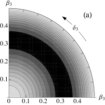
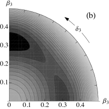
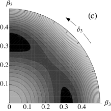
Figure 3: Three energy surfaces $E(\beta_{3},\delta_{3},\vartheta_{3}^{*},\varphi_{3}^{*})$ obtained in the classical limit of two different Hamiltonians of the $sf$-IBM for $N=6$ bosons. The values of $\vartheta_{3}$ and $\varphi_{3}$ are fixed and the dependence on $\beta_{3}>0$ and $0\leq\delta_{3}\leq{\frac{1}{2}}\pi$ is shown. Black corresponds to low energies and the lines indicate changes by 10 keV. (a) The ${\rm U}_{f}(7)$–${\rm SO}_{sf}(8)$ transitional Hamiltonian is taken with the parameters given in the caption of Fig. 2. (b) and (c) The Hamiltonian of (a) is modified by taking a repulsive interaction $v_{ffff}^{2}=500$ keV. The energy surface is shown for (b) $\vartheta_{3}^{*}={\frac{1}{2}}\pi$ and $\varphi_{3}^{*}=0$, and for (c) $\vartheta_{3}^{*}={\frac{1}{2}}\pi$ and $\varphi_{3}^{*}={\frac{1}{4}}\pi$.

The parameters quoted in the caption of Fig. 3 satisfy the conditions (44) and, as a result, the energy surface in the classical limit of the corresponding Hamiltonian displays an octupole-deformed minimum. According to the preceding discussion, the energy surface is independent of $\delta_{3}$ unless the matrix element $v_{ffff}^{2}$ is made repulsive, in which case an isolated tetrahedral minimum develops. This is indeed confirmed by the surfaces shown in Fig. 3, obtained by taking the classical limit of two different Hamiltonians of the $sf$-IBM. For display purposes the values of $\vartheta_{3}$ and $\varphi_{3}$ are fixed and the dependence on $\beta_{3}>0$ and $0\leq\delta_{3}\leq{\frac{1}{2}}\pi$ is shown. The classical limit of the symmetry Hamiltonian (15), for which $v_{ffff}^{2}=2a_{f}+2b_{f}-18c_{f}$, displays an octupole-deformed minimum at $\beta_{3}^{*}\approx 0.32$ and no dependence of $\delta_{3}$, as shown in Fig. 3(a). The change to $v_{ffff}^{2}=500$ keV introduces a minimum with tetrahedral symmetry ($\delta_{3}^{*}={\frac{1}{2}}\pi$) as shown in Fig. 3(b) for $\vartheta_{3}^{*}={\frac{1}{2}}\pi$ and $\varphi_{3}^{*}=0$, and in Fig. 3(c) for $\vartheta_{3}^{*}={\frac{1}{2}}\pi$ and $\varphi_{3}^{*}={\frac{1}{4}}\pi$. The latter energy surfaces display a second minimum with axially symmetric octupole deformation ($\delta_{3}^{*}=0$).

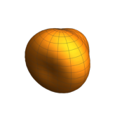
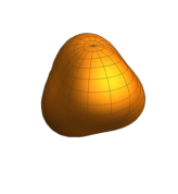
Figure 4: Energy spectrum of a general Hamiltonian of the $sf$-IBM for $N=6$ bosons. The same Hamiltonian is taken as in Fig. 2 but one $f$-boson two-body matrix element is modified to $v_{ffff}^{2}=500$ keV. On the left- and right-hand sides are shown the shapes at the minima in the energy surface obtained in the classical limit of this Hamiltonian. The shape on the left is axially symmetric, octupole deformed while the shape on the right has tetrahedral symmetry.

Although this proves that shapes with tetrahedral symmetry may occur with a reasonable parameterization in the $sf$-IBM, it is to be expected that the minimum is rather shallow as it occurs as a result of fine-tuning of little-known $f$-boson interactions. Even with a value as large as $v_{ffff}^{2}=500$ keV, the tetrahedral ($\delta_{3}^{*}={\frac{1}{2}}\pi$) and the axially symmetric ($\delta_{3}^{*}=0$) minima are separated by a barrier of only $\sim 20$ keV. As a result, only minute observable effects can be expected. This is illustrated in Fig. 4, which shows the spectrum of the ${\rm U}_{f}(8)$–${\rm SO}_{sf}(8)$ transitional Hamiltonian with the modified $v_{ffff}^{2}$ matrix element. Not much difference from the spectrum shown in Fig. 2 can be seen.

7 Conclusions

Two dynamical symmetries of the $sf$-IBM have been established: the ${\rm U}_{f}(7)$ limit with octupole vibrational characteristics and the ${\rm SO}_{sf}(8)$ limit where $s$- and $f$-boson states are mixed through an $sf$-pairing interaction, which, if strong enough, drives the system towards a permanent octupole deformation. This picture is confirmed by a catastrophe analysis of the energy surface obtained in the classical limit of a Hamiltonian transitional between the two limits, indicating that an octupole-deformed minimum can be obtained with reasonable single-boson energies. However, this minimum is always $\delta_{3}$ independent and shapes ranging from pear-like to tetrahedral are degenerate in energy. An isolated minimum with tetrahedral symmetry can be obtained by modifying two-body interactions between the $f$ bosons to the transitional symmetry Hamiltonian. It is separated from another minimum with axial symmetry by a low-energy barrier, even for fairly strong interactions between the $f$ bosons.

There are striking similarities between the search for tetrahedral shapes presented in this paper and the corresponding search for octahedral shapes reported in I and II. In both cases it is found that no isolated minimum with a higher-rank discrete symmetry is possible for a symmetry Hamiltonian of U(8) or U(15) but that a degenerate minimum occurs in the ${\rm SO}_{sf}(8)$ or ${\rm SO}_{sg}(10)$ limits of $sf$- or $sg$-pairing, respectively. An isolated minimum with tetrahedral or octahedral symmetry can be obtained through a modification of the two-body interaction between the relevant bosons. However, the minima thus constructed are rather shallow, even for large repulsive matrix elements between the $f$ or $g$ bosons, and their effects on spectroscopic properties are expected to be minute.

With this series of papers the role of higher-rank discrete symmetries in the context of algebraic nuclear models is clarified and a well-defined procedure is established to find out whether a given Hamiltonian of a particular version of the interacting boson model displays in its classical limit a minimum with a tetrahedral or octahedral shape. This enables the study of observable consequences of higher-rank discrete symmetries in the framework of algebraic models.

The limitations of this series of papers should nevertheless be recognized because the present analysis is restricted to Hamiltonians with up to two-body terms. It is possible that, just as triaxial shapes require higher-order interactions in the $sd$-IBM, shapes with a higher-rank discrete symmetry can be isolated with a high barrier by introducing higher-order interactions in $sdg$-IBM and $sf$-IBM. Also, as mentioned in the introduction of this paper, the analysis of the tetrahedral case so far has been limited to $sf$-IBM and should be carried out in the more general $spdf$-IBM. What can be concluded from the examples reported in this series of papers is that, unless such more complicated Hamiltonians are adopted, it will be difficult to identify clear effects of higher-rank discrete symmetries in nuclei.

References

• [1] P. Van Isacker, A. Bouldjedri, S. Zerguine, Nucl. Phys. A 938 (2015) 45.
• [2] A. Bouldjedri, S. Zerguine, P. Van Isacker, previous paper.
• [3] F. Iachello, A. Arima, The Interacting Boson Model, Cambridge University Press, Cambridge, 1987.
• [4] X. Li, J. Dudek, Phys. Rev. C 49 (1994) 1250(R).
• [5] J. Dudek, A. Góźdź, N. Schunck, M. Miśkiewicz, Phys. Rev. Lett. 88 (2002) 252502.
• [6] J. Dudek, D. Curien, N. Dubray, J. Dobaczewski, V. Pangon, P. Olbratowski, N. Schunck, Phys. Rev. Lett. 97 (2006) 072501.
• [7] P.A. Butler and W. Nazarewicz, Rev. Mod. Phys. 68 (1996) 349.
• [8] L.P. Gaffney et al., Nature 497 (2013) 199.
• [9] A. Arima, F. Iachello, Ann. Phys. (NY) 99 (1976) 253.
• [10] A. Arima, F. Iachello, Ann. Phys. (NY) 111 (1978) 201.
• [11] O. Scholten, F. Iachello, A. Arima, Ann. Phys. (NY) 115 (1978) 325.
• [12] J. Engel, F. Iachello, Phys. Rev. Lett. 54 (1985) 1126.
• [13] J. Engel, F. Iachello, Nucl. Phys. A 472 (1987) 61.
• [14] D. Kusnezov, J. Phys. A: Math. Gen.  22 (1989) 4271.
• [15] D. Kusnezov, J. Phys. A: Math. Gen. 23 (1990) 5673.
• [16] A. Bohr, Mat. Fys. Medd. Dan. Vid. Selsk. 26 (1952) no 14.
• [17] A. Bohr, B.R. Mottelson, Mat. Fys. Medd. Dan. Vid. Selsk. 27 (1953) no 16.
• [18] A. Bohr, B.R. Mottelson, Nuclear Structure. II Nuclear Deformations, Benjamin, New York, 1975.
• [19] S.G. Rohoziński, Rep. Prog. Phys. 51 (1988) 541.
• [20] I. Hamamoto, X.-Z. Zhang, H.-X. Xie, Phys. Lett. B 257 (1991) 1.
• [21] J. Dudek, A. Góźdź, N. Schunck, Acta Phys. Pol. B 34 (2003) 2491.
• [22] J. Dudek, A. Góźdź, K. Mazurek, H. Molique, J. Phys. G 37 (2010) 064032.
• [23] G. Racah, Phys. Rev. 76 (1949) 1352.
• [24] H. Weyl, The Classical Groups, Princeton University Press, Princeton, 1939.
• [25] A. Gheorghe, A.A. Raduta, J. Phys. A: Math. Gen. 37 (2004) 10951.
• [26] S.G. Rohoziński, J. Phys. G: Nucl. Phys. 4 (1988) 1075.
• [27] P. Van Isacker, S.  Heinze, Ann. Phys. (NY) 349 (2014) 73.
• [28] R. Gilmore, J. Math. Phys. 20 (1979) 891.
• [29] J.N. Ginocchio, M.W. Kirson, Phys. Rev. Lett.  44 (1980) 1744.
• [30] A.E.L. Dieperink, O. Scholten, F. Iachello, Phys. Rev. Lett.  44 (1980) 1747.
• [31] The $\mu=0$ term is treated here separately to avoid the double counting in Eq. (12) of I.
• [32] J.N. Ginocchio, M.W. Kirson, Nucl. Phys. A 350 (1980) 31.
• [33] P. Van Isacker, J.-Q. Chen, Phys. Rev. C 24 (1981) 684.
• [34] A. Arima, F. Iachello, Ann. Phys. (NY) 123 (1979) 468.