Ancient solutions of the homogeneous Ricci flow on flag manifolds

Abstract.

For any flag manifold $M=G/K$ of a compact simple Lie group $G$ we describe non-collapsing ancient invariant solutions of the homogeneous unnormalized Ricci flow. Such solutions emerge from an invariant Einstein metric on $M$, and by [BöLS17] they must develop a Type I singularity in their extinction finite time, and also to the past. To illustrate the situation we engage ourselves with the global study of the dynamical system induced by the unnormalized Ricci flow on any flag manifold $M=G/K$ with second Betti number $b_{2}(M)=1$, for a generic initial invariant metric. We describe the corresponding dynamical systems and present non-collapsed ancient solutions, whose $\alpha$-limit set consists of fixed points at infinity of $\operatorname{\mathscr{M}}^{G}$. Based on the Poincaré compactification method, we show that these fixed points correspond to invariant Einstein metrics and we study their stability properties, illuminating thus the structure of the system’s phase space.

Introduction

Given a Riemannian manifold $(M^{n},g)$, recall that the unnormalized Ricci flow is the geometric flow defined by

$$\frac{\partial g(t)}{\partial t}=-2\operatorname{\mathsf{Ric}}_{g(t)}\,,\quad g(0)=g\,,$$ (0.1)

where $\operatorname{\mathsf{Ric}}_{g(t)}$ denotes the Ricci tensor of the one-parameter family $g(t)$. The above system consists of non-linear second order partial differential equations on the open convex cone $\operatorname{\mathscr{M}}$ of Riemannian metrics on $M$. A smooth family $\{g(t):t\in[0,T)\subset\mathbb{R}\}\in\operatorname{\mathscr{M}}$ defined for some $0<T\leq\infty$, is said to be a solution of the Ricci flow with initial metric $g$, if it satisfies the system (0.1) for any $x\in M$ and $t\in[0,T)$. The Ricci flow was introduced in the celebrated work of Hamilton [H82] and nowadays is the essential tool in the proof of the famous Poincaré conjecture and Thurston’s geometrization conjecture, due to the seminal works [P02, P03] of G. Perelman.

In general, and since a system of partial differential equations is involved, it is hard to produce explicit examples of Ricci flow solutions. However, the Ricci flow for an initial invariant metric reduces to a system of ODEs. More precisely, homogeneity implies bounded curvature (see [ChZ06]), and thus the isometries of the initial metric will be in fact the isometries of any involved metric. Hence, when $g$ is an invariant metric, any solution $g(t)$ of (0.1) is also invariant. As a result, in some cases it is possible to solve the system explicitly and proceed to a study of their asymptotic properties, or even specify analytical properties related to different type of singularities and deduce curvature estimates, see [BöW07, GM09, AnC11, GM12, Buz14, Laf15, Bö15, BöLS17, AbN16, GMPSS20], and the articles quoted therein. Especially for the non-compact case, note that during the last decade the Ricci flow for homogeneous, or cohomogeneity-one metrics, together with the so-called bracket flow play a key role in the study of the Alekseevsky conjecture, see [Pn10, L11a, L11b, L13, LL14a, LL14b, BöL18a, BöL18b].

In this work we examine the Ricci flow, on compact homogeneous spaces with simple spectrum of isotropy representation, in terms of Graev [Gr06, Gr13], or of monotypic isotropy representation, in terms of Buzano [Buz14], or Pulemotov and Rubinstein [PR19]. Nowadays, such spaces are of special interest due to their rich applications in the theory of homogeneous Einstein metrics, prescribed Ricci curvature, Ricci iteration, Ricci flow and other (see [A$\ell$P86, S99, Bö04, BöWZ04, Gr06, AC10, AC11, Buz14, Gr13, CS14, Bö15, PP15, PR19, GMPSS20]). Here, we focus on flag manifolds $M=G/K$ of a compact simple Lie group $G$ and examine the dynamical system induced by the vector field corresponding to the homogeneous Ricci flow equation. On such cosets (even for $G$ semisimple), the homogeneous Ricci flow cannot possess fixed (stationary) points, since by the theorem of Alekseevsky and Kimel’fel’d [A$\ell$K75] invariant Ricci flat metrics must be flat and so they cannot exist. However, as follows from the maximum principle, the homogeneous Ricci flow on any flag manifold $M=G/K$ must admit ancient invariant solutions, which in fact by the work of Böhm [Bö15] must have finite extinction time (note that since any flag manifold is compact and simply connected and carries invariant Einstein metrics, e.g. invariant Kähler-Einstein metrics always exist, the first conclusion above occurs also by a result of Lafuente [Laf15, Cor. 4.3]).

To be more specific, recall that a solution $g(t)$ of the Ricci flow is called ancient if it has as interval of definition the open set $(-\infty,T)$, for some $T<\infty$. Such solutions are important, because they arise as limits of blow ups of singular solutions to the Ricci flow near finite time singularities, see [EMT11]. For our case it follows that for any flag manifold $M=G/K$ one must be always able to specify a $G$-invariant metric $g$, such that any (maximal) Ricci flow solution $g(t)$ with initial condition $g(0)=g$ has an interval of definition of the form $(t_{a},T)$, with $-\infty\leq t_{a}<0$ and $T<\infty$. Indeed, for any flag space below we will provide explicit solutions of this type, which are ancient; They arise by using an invariant Kähler-Einstein metric, which always exists, or any other possible existent invariant Einstein metric $g_{0}$, and they are defined on open intervals of the form $(-\infty,T)$, where

$$T=\frac{1}{2\lambda}=\frac{n}{2}\operatorname{\mathsf{Scal}}(g_{0})^{-1},$$

with $\lambda=\frac{\operatorname{\mathsf{Scal}}(g_{0})}{n}>0$ being the corresponding Einstein constant (see Proposition 2.4). All such solutions become extinct when $t\to T$, in the sense that $g(t)\to 0$, i.e. they tend to $0$. As ancient solutions, they have positive scalar curvature $\operatorname{\mathsf{Scal}}(g(t))$ ([Ch09]) and the asymptotic behaviour of $\operatorname{\mathsf{Scal}}(g(t))$, at least for the trivial one, can be easily treated, see Proposition 2.4 which forms a specification of [Laf15, Thm. 1.1] on flag manifolds (see also Examples 3.3, 3.4). Moreover, for any invariant Einstein metric on $M=G/K$ with $b_{2}(M)=1$, we show the existence of an unstable manifold and compute its dimension. For the invariant Einstein metrics which are not Kähler, we obtain a 2- or 3-dimensional unstable manifold, depending on the specific case, which implies the existence of non–trivial ancient solutions emerging from the corresponding Einstein metric. Actually, by [BöLS17], it also follows that these ancient solutions develop a Type I singularity. This means (see [EMT11, Buz14, Bö15, LW17])

$$\lim_{t\to-\infty}\Big{(}|t|\cdot{\rm sup}_{x\in M}\|\mathsf{Rm}(g(t))\|_{g(t)}(x,t)\Big{)}<\infty\,,$$

where $\mathsf{Rm}(g(t))$ denotes the curvature tensor of $(M=G/K,g(t))$, or equivalently that there is a constant $0<C_{g_{0}}<\infty$ such that $(T-t)\cdot{\rm sup}_{M}\|\mathsf{Rm}(g(t))\|_{g(t)}\leq C_{g_{0}}$, for any $t\in(-\infty,T=\frac{1}{2\lambda})$. Finally, by [BöLS17] we also deduce that the predicted non-trivial ancient solutions are non-collapsed (and the same the trivial one, see Corollary 2.8). In this point we should mention that not any compact homogeneous space $M=G/K$ of a compact (semi)simple Lie group $G$ admits (unstable) Einstein metrics (see for example [WZ86, PS97] for non-existence results). So, even assuming that the universal covering of $M^{n}=G/K$ is not diffeomorphic to $\operatorname{\mathbb{R}}^{n}$ (which for the compact case is equivalent to say that $M^{n}$ is not a $n$-torus), the predicted solutions of Lafuente can be in general hard to be specified.

Note now that for any flag manifold $M=G/K$ of a compact simple Lie group $G$, the symmetric space of invariant metrics $\operatorname{\mathscr{M}}^{G}$ is the phase space of the homogeneous Ricci flow and it is flat, i.e. $\operatorname{\mathscr{M}}^{G}\cong\operatorname{\mathbb{R}}^{r}_{+}$ for some $r\geq 1$. Therefore, the dynamical system of the homogeneous Ricci flow can be converted to a qualitative equivalent dynamical system of homogeneous polynomial equations and the well-known Poincaré compactification ([P1891]) strongly applies. The main idea back of this method is to identify $\operatorname{\mathbb{R}}^{n}$ with the northern and southern hemispheres through central projections, and then extend $X$ to a vector field $p(X)$ on $\operatorname{\mathsf{S}}^{n}$ (see Section 2.2). Here, for any (non-symmetric) flag manifold $M=G/K$ of a compact simple Lie group $G$ with $b_{2}(M)=1$, we present the global study of the dynamical system induced by the vector field corresponding to the unnormalized Ricci flow for an initial invariant metric, which is generic. In particular, the main contribution of this work is the description via the Poincaré compactification method, of the fixed points of the homogeneous Ricci flow at the so-called infinity of $\operatorname{\mathscr{M}}^{G}$ (see Definition 2.11 and Remark 2.13). Based on this method we can study the stability properties of such fixed points, which we prove that are in bijective correspondence with the existent invariant Einstein metrics on $M=G/K$, and moreover that coincide with the $\alpha$-limit set of an invariant line, i.e. a solution of the homogeneous Ricci flow which has as trace a line of $\operatorname{\mathscr{M}}^{G}$. It turns out that such solutions are ancient and non-collapsed, and develop Type I singularities. Note that through the compactification procedure of Poincaré, we are able to distinguish the unique invariant Kähler-Einstein metric from the other invariant Einstein metrics in terms of (un)stable manifolds, in particular for every invariant Einstein metric we compute the dimension of the corresponding (un)stable manifold. Moreover, for the case $r=2$ we discuss the $\omega$-limit of any solution of the homogeneous Ricci flow, for details see Theorem 3.1. Since we are interested in the unnormalized Ricci flow on flag manifolds with $b_{2}(M)=1$, we should finally mention that this dynamical system has been very recently examined by [GMPSS20], for flag spaces with three isotropy summands (however via a different method of the Poincaré compactification), while a related study of certain examples of flag manifolds with two isotropy is given in [GM12]. Note finally that for flag manifolds with $r=2$, this work is complementary to [Buz14], in the sense that there were studied homogeneous ancient solutions on compact homogeneous spaces with two isotropy summands; However, the specific class of flag manifolds with $r=2$ was excluded (see at the end of the article [Buz14]), and the filling of this small gap was a motivation of the present work.

The structure of the paper is given as follows: In Section 1 we refresh basics from the theory of homogeneous spaces, introduce the homogeneous Ricci flow and recall some details from the structure and geometry of flag manifolds. Next, in Section 2 we shortly present some basic results for ancient solutions emerging from an invariant Einstein metric, and also the Poincaré compactification adapted to our scopes. Finally, Section 3 is about the global study of the homogeneous Ricci flow for all non-symmetric flag manifolds $M=G/K$ of a compact simple Lie group $G$ with $b_{2}(M)=1$, where a proof of our main theorem, i.e. Theorem 3.1, is presented.

Acknowledgements: The authors are grateful to C. Böhm, R. Lafuente and Y. Sakane for insightful comments. They also thank J. Lauret and C. E. Will for their remarks and pointing out a mistake in the main Theorem 3.1 in a previous draft of this manuscript. I. C. acknowledges support by Czech Science Foundation, via the project GAČR no. 19-14466Y. S. A. thanks the University of Hradec Králové for hospitality along a research stay in September 2019.

1. Preliminaries

We begin by recalling preliminaries of the homogeneous Ricci flow. After that we will refresh useful notions of the structure and geometry of generalized flag manifolds.

1.1. Homogeneous Ricci flow

Recall that a homogeneous Riemannian manifold is a homogeneous space $M=G/K$ (see [KN69, CE75, A$\ell$VL91] for details on homogeneous spaces) endowed with a $G$-invariant metric $g$, that is $\tau_{a}^{*}g=g$ for any $a\in G$, where $\tau:G\times G/K\to G/K$ denotes the transitive $G$-action. Equivalently, is a Riemannian manifold $(M,g)$ endowed with a transitive action of its isometry group $\operatorname{\mathsf{Iso}}(M,g)$. If $M$ is connected, then each closed subgroup $G\subseteq\operatorname{\mathsf{Iso}}(M,g)$ which is transitive on $M$ induces a presentation of $(M,g)$ as a homogeneous space, i.e. $M=G/K$, where $K\subset G$ is the stabilizer of some point $o\in M$. In this case, the transitive Lie group $G$ can be also assumed to be connected (since the connected component of the identity of $G$ is also transitive on $M$). Usually, to emphasize on the transitive group $G$, we say that $(M,g)$ is a $G$-homogeneous Riemannian manifold. However, note that may exist many closed subgroups of $\operatorname{\mathsf{Iso}}(M,g)$ acting transitively on $(M,g)$. Next we shall work with connected homogeneous manifolds.

As it is well-known, the geometric properties of a homogeneous space can be examined by restricting our attention to a point. Set $o=eK$ for the identity coset of $(M^{n}=G/K,g)$ and let $T_{o}G/K$ be the corresponding tangent space. Since we assume the existence of a $G$-invariant metric $g$, $K\subset G$ can be identified with a closed subgroup of $\operatorname{\mathsf{O}}(n)\equiv\operatorname{\mathsf{O}}(T_{o}G/K)$ (or of $\operatorname{\mathsf{SO}}(n)$ if $G/K$ is oriented), so $K$ is compact and hence any homogeneous Riemannian manifold $(M^{n}=G/K,g)$ is a reductive homogeneous space. This means that there is a complement $\mathfrak{m}$ of the Lie algebra $\mathfrak{k}=\operatorname{\mathsf{Lie}}(K)$ of the stabilizer $K$ inside the Lie algebra $\mathfrak{g}=\operatorname{\mathsf{Lie}}(G)$ of $G$, which is $\operatorname{Ad}_{G}(K)$-invariant, i.e. $\mathfrak{g}=\mathfrak{k}\oplus\mathfrak{m}$ and $\operatorname{Ad}_{G}(K)\mathfrak{m}\subset\mathfrak{m}$, where $\operatorname{Ad}_{G}\equiv\operatorname{Ad}:G\to\operatorname{\mathsf{Aut}}(\mathfrak{g})$ denotes the adjoint representation of $G$. Note that in general the reductive complement $\mathfrak{m}$ may not be unique, and for a general homogeneous space $G/K$ a sufficient condition for its existence is the compactness of $K$. On the other hand, once such a decomposition has been fixed, there is always a natural identification of $\mathfrak{m}$ with the tangent space $T_{o}G/K=\mathfrak{g}/\mathfrak{k}$, given by

$$X\in\mathfrak{m}\longleftrightarrow X^{*}_{o}=\frac{d}{dt}\big{|}_{t=0}\tau_{\exp tX}(o)\in T_{o}G/K\,,$$

where $\exp tX$ is the one-parameter subgroup of $G$ generated by $X$. Under the linear isomorphism $\mathfrak{m}=T_{o}G/K$, the isotropy representation $\chi:K\to\operatorname{\mathsf{Aut}}(\mathfrak{m})$, defined by $\chi(k):=(d\tau_{k})_{o}$ for any $k\in K$, is equivalent with the representation $\operatorname{Ad}_{G}|_{K}:K\times\mathfrak{m}\to\mathfrak{m}$. Hence, $\chi(k)X=\operatorname{Ad}_{G}(k)X$ for any $k\in K$ and $X\in\mathfrak{m}$. In terms of Lie algebras we have $\chi_{*}(Y)X=[Y,X]_{\mathfrak{m}}$ for any $Y\in\mathfrak{k}$ and $X\in\mathfrak{m}$, or in other words $\chi_{*}(Y)=\operatorname{ad}(Y)|_{\mathfrak{m}}$.

The homogeneous spaces $M=G/K$ that we will examine below (with $K$ compact), are assumed to be almost effective, which means that the kernel $\operatorname{\mathsf{Ker}}(\tau)$ (which is a normal subgroup both of $G$ and $K$), is finite. Thus, the isotropy representation $\chi$ is assumed to have a finite kernel, and then we may identify $\mathfrak{k}$ with the Lie algebra $\chi_{*}(\mathfrak{k})=\operatorname{\mathsf{Lie}}(\chi(K))$ of the linear isotropy group $\chi(K)\subset\operatorname{\mathsf{Aut}}(\mathfrak{m})$. When only the identity element $e\in G$ acts as the identity transformation on $M=G/K$, then the $G$-action is called effective and the isotropy representation $\chi$ is injective. If we assume for example that $G\subseteq\operatorname{\mathsf{Iso}}(M,g)$ is a closed subgroup, then the action of $G$ to $G/K$ is effective. Note that an almost effective action of $G$ on $G/K$ gives rise to an effective action of the group $G^{\prime}=G/\operatorname{\mathsf{Ker}}(\tau)$ (of the same dimension with $G$), so we will not worry much for the effectiveness of $M=G/K$.

Recall that the space of $G$-invariant symmetric covariant 2-tensors on a (almost) effective homogeneous space $M=G/K$ with a reductive decomposition $\mathfrak{g}=\mathfrak{k}\oplus\mathfrak{m}$, is naturally isomorphic with the space of symmetric bilinear forms on $\mathfrak{m}$, which are invariant under the isotropy action of $K$ on $\mathfrak{m}$. As a consequence, the space $\operatorname{\mathscr{M}}^{G}$ of $G$-invariant Riemannian metrics on $M=G/K$ coincides with the space of inner products $\langle\ ,\ \rangle$ on $\mathfrak{m}$ satisfying

$$\langle X,Y\rangle=\langle\chi(k)X,\chi(k)Y\rangle=\langle\operatorname{Ad}_{G}(k)X,\operatorname{Ad}_{G}(k)Y\rangle\,,$$

for any $k\in K$ and $X,Y\in\mathfrak{m}$. The correspondence is given by $\langle X,Y\rangle=g(X,Y)_{o}$. Moreover, when $K$ is compact and $\mathfrak{m}=\mathfrak{h}^{\perp}$ with respect to $B=-B_{\mathfrak{g}}$, where $B_{\mathfrak{g}}$ is the Killing form of $\mathfrak{g}$, then one can extend the above correspondence between elements $g=\langle\ ,\ \rangle\in\operatorname{\mathscr{M}}^{G}$ and $\operatorname{Ad}_{G}(K)$-invariant $B$-selfadjoint positive-definite endomorphisms $L:\mathfrak{m}\to\mathfrak{m}$ of $\mathfrak{m}$, i.e. $\langle X,Y\rangle=B(LX,Y)$, for any $X,Y\in\mathfrak{m}$. To simplify the text, whenever is possible next we shall relax the notation $\operatorname{Ad}_{G}(K)$ to $\operatorname{Ad}(K)$ and scalar products on $\mathfrak{m}$ as above, will be just referred to as $\operatorname{Ad}(K)$-invariant scalar products. Note that the $\operatorname{Ad}(K)$-invariance of $\langle\ ,\ \rangle$ implies its $\operatorname{ad}(\mathfrak{k})$-invariance, which means that the endomorphism $\operatorname{ad}(Z)|_{\mathfrak{m}}:\mathfrak{m}\to\mathfrak{m}$ is skew-symmetric with respect to $\langle\ ,\ \rangle$, for any $Z\in\mathfrak{k}$. When $K$ is connected, the inclusions $\operatorname{Ad}(k)\mathfrak{m}\subset\mathfrak{m}$ and $[\mathfrak{k},\mathfrak{m}]\subset\mathfrak{m}$ are equivalent and hence one can pass from the $\operatorname{Ad}(K)$-invariance to $\operatorname{ad}(\mathfrak{k})$-invariance and conversely. From now on will denote by $P(\mathfrak{m})^{\operatorname{Ad}(K)}$ the space of all $\operatorname{Ad}(K)$-invariant inner products on $\mathfrak{m}$.

Given a Riemannian manifold $(M^{n},g)$, a solution of the Ricci flow is a family of Riemannian metrics $\{g_{t}\}\in\operatorname{\mathscr{M}}$ satisfying the system (0.1). If the initial metric $g=g(0)\in\operatorname{\mathscr{M}}$ is a $G$-invariant metric with respect to some closed subgroup $G\subseteq\operatorname{\mathsf{Iso}}(M,g)$, i.e. $(M=G/K,g)$ is a homogeneous Riemannian manifold and so $g\in\operatorname{\mathscr{M}}^{G}$, then the solution $\{g(t)\}$ is called homogeneous, i.e. $\{g(t)\}\in\operatorname{\mathscr{M}}^{G}$. Indeed, the isometries of $g$ are isometries for any other evolved metric, and by [Kot10] it is known that the isometry group is preserved under the Ricci flow. Thus, after considering a reductive decomposition $\mathfrak{g}=\mathfrak{k}\oplus\mathfrak{m}$ of $(M=G/K,g)$, the homogeneity of $g$ allows us to reduce the Ricci flow to a system of ODEs for a curve of $\operatorname{Ad}(K)$-invariant inner products on $P(\mathfrak{m})^{\operatorname{Ad}(K)}$, where $\mathfrak{m}\cong T_{o}G/K$ is a reductive complement. In particular, due to the identification $\operatorname{\mathscr{M}}^{G}\cong P^{\operatorname{Ad}(K)}(\mathfrak{m})$ we may write $g(t)=\langle\ ,\ \rangle_{t}$ and then (0.1) takes the form

$$\frac{d}{dt}\langle\ ,\ \rangle_{t}=-2\operatorname{\mathsf{Ric}}_{\langle\ ,\ \rangle_{t}}\,,\quad\langle\ ,\ \rangle_{0}\equiv\langle\ ,\ \rangle=g\,,$$

where $\operatorname{\mathsf{Ric}}_{\langle\ ,\ \rangle_{t}}$ denotes the $\operatorname{Ad}(K)$-invariant bilinear form on $\mathfrak{m}$, corresponding to the Ricci tensor of $g(t)$. Note that since $g_{0}=g(0)$ is an invariant metric, the solution $g(t)$ of (0.1) must be unique among complete, bounded curvature metrics (see [ChZ06]).

Remark 1.1.

When one is interested in more general homogeneous spaces $M=G/K$ and a reductive decomposition may not exist, the above setting can be appropriately transferred to $\mathfrak{g}/\mathfrak{k}\cong T_{o}G/K$. However, the “reductive setting” serves well the goals of this paper and it is sufficient for our subsequent computations and description.

1.2. Flag manifolds

Let $G$ be a compact semisimple Lie group with Lie algebra $\operatorname{\mathsf{Lie}}(G)=\mathfrak{g}$. A flag manifold is an adjoint orbit of $G$, i.e.

$$M=\operatorname{Ad}(G)w=\{\operatorname{Ad}(G)w:g\in G\}\subset\mathfrak{g}$$

for some left-invariant vector field $w\in\mathfrak{g}$. Let $K=\{g\in G:\operatorname{Ad}(g)w=w\}\subset G$ be the isotropy subgroup of $w$ and let $\mathfrak{k}=\operatorname{\mathsf{Lie}}(K)$ be the corresponding Lie algebra. Since $G$ acts on $M$ transitively, $M$ is diffeomorphic to the (compact) homogeneous space $G/K$, that is $\operatorname{Ad}(G)w=G/K$. In particular, $\mathfrak{k}=\{X\in\mathfrak{g}:[X,w]=0\}=\ker\operatorname{ad}(w)$, where $\operatorname{ad}:\mathfrak{g}\to\operatorname{End}(\mathfrak{g})$ is the adjoint representation of $\mathfrak{g}$. Moreover, the set $S_{w}=\overline{\{\exp(tw):t\in\mathbb{R}\}}$ is a torus in $G$ and the isotropy subgroup $K$ is identified with the centralizer in $G$ of $S_{w}$, i.e. $K=C(S_{w})$. Hence $\operatorname{\mathsf{rank}}G=\operatorname{\mathsf{rank}}K$ and $K$ is connected. Thus, equivalently a flag manifold is a homogeneous space of the form $G/K$, where $K=C(S)=\{g\in G:ghg^{-1}=h\ \mbox{for all}\ h\in S\}$ is the centralizer of a torus $S$ in $G$. When $K=C(T)=T$ is the centralizer of a maximal torus $T$ in $G$, the $G/T$ is called a full flag manifold. Flag manifolds admit a finite number of invariant complex structures, in particular flag spaces $G/K$ of a compact, simply connected, simple Lie group $G$ exhaust all compact, simply connected, de Rham irreducible homogeneous Kähler manifolds (see for example [A$\ell$P86, AC10, C12, A$\ell$C19] for further details).

So, for any flag manifold $M=G/K$ we may work with $G$ simply connected (if for instance a flag manifold of $\operatorname{\mathsf{SO}}(n)$ is given, one can always pass to its universal covering by using the double covering $\operatorname{\mathsf{Spin}}(n)$). For our scopes, it is also sufficient to focus on the de Rham irreducible case, which is equivalent to say that $G$ is simple, see [KN69]. Hence, in the following we can always assume that $M=G/K$ satisfies these conditions, and as before we shall denote by $B_{\mathfrak{g}}$ the Killing form of the Lie algebra $\mathfrak{g}$. The $\operatorname{Ad}(G)$-invariant inner product $B:=-B_{\mathfrak{g}}$ induces a bi-invariant metric on $G$ by left translations, and we may fix, once and for all, a $B$-orthogonal $\operatorname{Ad}(K)$-invariant decomposition $\mathfrak{g}=\mathfrak{k}\oplus\mathfrak{m}$. $G$-invariant Riemannian metrics on $G/K$ will be identified with $\operatorname{Ad}(K)$-invariant inner products $\langle\ ,\ \rangle$ on the reductive complement $\mathfrak{m}=T_{o}G/K$. Note that the restriction $B\big{|}_{\mathfrak{m}}$ induces the so-called Killing metric $g_{B}\in\operatorname{\mathscr{M}}^{G}$, which is the unique invariant metric for which the natural projection $\pi:(G,B)\longrightarrow(G/K,g_{B})$ is a Riemannian submersion.

The second Betti number of any flag manifold $M=G/K$ is encoded in the corresponding painted Dynkin diagram. To recall the procedure, let $\mathfrak{g}^{\mathbb{C}}=\mathfrak{h}^{\mathbb{C}}\oplus\sum_{\alpha\in R}\mathfrak{g}_{\alpha}^{\mathbb{C}}$ be the usual root space decomposition of the complexification $\mathfrak{g}^{\mathbb{C}}$ of $\mathfrak{g}$, with respect to a Cartan subalgebra $\mathfrak{h}^{\mathbb{C}}$ of $\mathfrak{g}^{\mathbb{C}}$, where $R\subset(\mathfrak{h}^{\mathbb{C}})^{*}$ is the root system of $\mathfrak{g}^{\mathbb{C}}$. Via the Killing form of $\mathfrak{g}^{\operatorname{\mathbb{C}}}$ we identify $(\mathfrak{h}^{\mathbb{C}})^{*}$ with $\mathfrak{h}^{\mathbb{C}}$. Let $\Pi=\{\alpha_{1},\ldots,\alpha_{\ell}\}$  $(\dim\mathfrak{h}^{\mathbb{C}}=\ell)$ be a fundamental system of $R$ and choose a subset $\Pi_{K}$ of $\Pi$. We denote by $R_{K}=\{\beta\in R:\beta=\sum_{\alpha_{i}\in\Pi_{K}}k_{i}\alpha_{i}\}$ the closed subsystem spanned by $\Pi_{K}$. Then, the Lie subalgebra $\mathfrak{k}^{\mathbb{C}}=\mathfrak{h}^{\mathbb{C}}\oplus\sum_{\beta\in R_{K}}\mathfrak{g}_{\beta}^{\mathbb{C}}$ is a reductive subalgebra of $\mathfrak{g}^{\mathbb{C}}$, i.e. it admits a decomposition of the form $\mathfrak{k}^{\mathbb{C}}=Z(\mathfrak{k}^{\mathbb{C}})\oplus\mathfrak{k}_{ss}^{\mathbb{C}}$, where $Z(\mathfrak{k}^{\mathbb{C}})$ is its center and $\mathfrak{k}_{ss}^{\mathbb{C}}=[\mathfrak{k}^{\mathbb{C}},\mathfrak{k}^{\mathbb{C}}]$ the semisimple part of $\mathfrak{k}^{\mathbb{C}}$. In particular, $R_{K}$ is the root system of $\mathfrak{k}^{\mathbb{C}}_{ss}$, and thus $\Pi_{K}$ can be considered as the associated fundamental system. Let $K$ be the connected Lie subgroup of $G$ generated by $\mathfrak{k}=\mathfrak{k}^{\mathbb{C}}\cap\mathfrak{g}$. Then the homogeneous manifold $M=G/K$ is a flag manifold, and any flag manifold is defined in this way, i.e., by the choise of a triple $(\mathfrak{g}^{\mathbb{C}},\Pi,\Pi_{K})$, see also [A$\ell$P86, AC10, C12, A$\ell$C19].

Set $\Pi_{M}=\Pi\backslash\Pi_{K}$ and $R_{M}=R\backslash R_{K}$, such that $\Pi=\Pi_{K}\sqcup\Pi_{M}$, and $R=R_{K}\sqcup R_{M}$, respectively. Roots in $R_{M}$ are called complementary roots. Let $\Gamma=\Gamma(\Pi)$ be the Dynkin diagram of the fundamental system $\Pi$.

Definition 1.2.

Let $M=G/K$ be a flag manifold. By painting black the nodes of $\Gamma$ corresponding to $\Pi_{M}$, we obtain the painted Dynkin diagram of $G/K$ (PDD in short). In this diagram the subsystem $\Pi_{K}$ is determined as the subdiagram of white roots.

Remark 1.3.

Conversely, given a PDD, one may determine the associated flag manifold $M=G/K$ as follows: The group $G$ is defined as the unique simply connected Lie group generated by the unique real form $\mathfrak{g}$ of the complex simple Lie algebra $\mathfrak{g}^{\mathbb{C}}$ (up to inner automorphisms of $\mathfrak{g}^{\mathbb{C}}$), which is reconstructed by the underlying Dynkin diagram. Moreover, the connected Lie subgroup $K\subset G$ is defined by using the encoded by the PDD splitting $\Pi=\Pi_{K}\sqcup\Pi_{M}$; The semisimple part of $K$ is obtained from the (not necessarily connected) subdiagram of white simple roots, while each black root, i.e. each root in $\Pi_{M}$, gives rise to a $\operatorname{\mathsf{U}}(1)$-summand. Thus, the PDD determines the isotropy group $K$ and the space $M=G/K$ completely. By using certain rules to determine whether different PDDs define isomorphic flag manifolds (see [A$\ell$P86]), one can obtain all flag manifolds $G/K$ of a compact simple Lie group $G$ (see for example the tables in [A$\ell$C19]).

Proposition 1.4.

([BH58, A$\ell$P86]) The second Betti number of a flag manifold $M=G/K$ equals to the totality of black nodes in the corresponding PDD, i.e. the cardinality of the set $\Pi_{M}$.

Note that for any flag manifold $M=G/K$, the $B$-orthogonal reductive complement $\mathfrak{m}$ decomposes into a direct sum of $\operatorname{Ad}(K)$-inequivalent and irreducible submodules, which we call isotropy summands, see [A$\ell$P86, AC10, A$\ell$C19] and the references therein. This means that when $\mathfrak{m}\cong T_{o}M$ is viewed as a $K$-module, then there is always a $B$-orthogonal $\operatorname{Ad}(K)$-invariant decomposition

$$\mathfrak{m}=\mathfrak{m}_{1}\oplus\cdots\oplus\mathfrak{m}_{r}\,,$$ (1.1)

for some $r\geq 1$, such that

• $K$ acts (via the isotropy representation) irreducibly on any $\mathfrak{m}_{1},\ldots,\mathfrak{m}_{r}$, and

• $\mathfrak{m}_{i}\ncong\mathfrak{m}_{j}$ are inequivalent as $\operatorname{Ad}(K)$-representations for any $i\neq j$.

In fact, a decomposition as in (1.1) satisfying the given conditions must be unique, up to a permutation of the isotropy summands, see for example [PR19]. When $r=1$, $M=G/K$ is an isotropy irreducible compact Hermitian symmetric space (HSS in short), and all these cosets can be viewed as flag manifolds with $b_{2}(M)=1$. Note that from the class of full flag manifolds only $\operatorname{\operatorname{\mathbb{C}}\mathsf{P}}^{1}\cong\operatorname{\mathsf{S}}^{2}=\operatorname{\mathsf{SU}}(2)/\operatorname{\mathsf{U}}(1)$ is an irreducible HSS, and hence a flag manifold with $b_{2}(M)=1$. In this text we are mainly interested in non-symmetric flag manifolds $M=G/K$ with $b_{2}(M)=1$, and in this case $r$ is bounded by the inequalities $2\leq r\leq 6$ (see below).

Lemma 1.5.

([A$\ell$P86, AC10]) Let $M=G/K$ be a flag manifold of a compact simple Lie group. Then, the isotropy representation of $M$ is monotypic and decomposes as in (1.1), for some $r\geq 1$. Moreover, any $G$-invariant metric on $M=G/K$ is given by

$$g=\langle\ ,\ \rangle=\sum_{i=1}^{r}x_{i}\cdot B|_{\mathfrak{m}_{i}}\,,$$ (1.2)

where $x_{i}\in\operatorname{\mathbb{R}}_{+}$ are positive real numbers for any $i=1,\ldots,r$. Thus, $\operatorname{\mathscr{M}}^{G}$ coincides with the open convex cone $\operatorname{\mathbb{R}}^{r}_{+}=\{(x_{1},\ldots,x_{r})\in\operatorname{\mathbb{R}}^{r}:x_{i}>0\ \text{for any}\ \ i=1\ldots r\}$.

Invariant metrics as in (1.2) are called diagonal (see [WZ86] for details). By Schur’s Lemma, the Ricci tensor $\operatorname{\mathsf{Ric}}_{g}$ of such a diagonal invariant metric $g$, needs to preserve the splitting (1.1) and consequently, $\operatorname{\mathsf{Ric}}_{g}$ is also diagonal, i.e. $\operatorname{\mathsf{Ric}}_{g}(\mathfrak{m}_{i},\mathfrak{m}_{j})=0$, whenever $i\neq j$. As before, $\operatorname{\mathsf{Ric}}_{g}$ is determined by a symmetric $\operatorname{Ad}(K)$-invariant bilinear form on $\mathfrak{m}$, although not necessarily positive definite, and hence it has the expression

$$\operatorname{\mathsf{Ric}}_{g}\equiv\operatorname{\mathsf{Ric}}_{\langle\ ,\ \rangle}=\sum_{i=1}^{r}y_{i}\cdot B\big{|}_{\mathfrak{m}_{i}}=\sum_{i=1}^{r}(x_{i}\cdot\operatorname{\mathsf{ric}}_{i})\cdot B\big{|}_{\mathfrak{m}_{i}}\,,$$

for some $y_{i}=x_{i}\cdot\operatorname{\mathsf{ric}}_{i}\in\mathbb{R}$, where $\langle\ ,\ \rangle\in P^{\operatorname{Ad}(K)}(\mathfrak{m})$ is the $\operatorname{Ad}(K)$-invariant inner product corresponding to $g\in\operatorname{\mathscr{M}}^{G}$ and $\operatorname{\mathsf{ric}}_{i}$ are the so-called Ricci components. There is a simple description of $\operatorname{\mathsf{ric}}_{i}$, and hence of $\operatorname{\mathsf{Ric}}_{g}$ (and also of the scalar curvature $\operatorname{\mathsf{Scal}}_{g}={\rm tr}\operatorname{\mathsf{Ric}}_{g})$, in terms of the metric parameters $x_{i}$, the dimensions $d_{i}=\dim_{\operatorname{\mathbb{R}}}\mathfrak{m}_{i}$ and the so-called structure constants of $G/K$ with respect to the decomposition (1.1),

$$c_{ij}^{k}\equiv{k\brack{i\ j}}=\sum_{\alpha,\beta,\gamma}B([X_{\alpha},Y_{\beta}],Z_{\gamma})^{2}\,,\quad i,j,k\in\{1,\ldots,r\},$$

where $\{X_{\alpha}\}$, $\{Y_{\beta}\}$, $\{Z_{\gamma}\}$ are $B$-orthonormal bases of $\mathfrak{m}_{i}$, $\mathfrak{m}_{j}$, $\mathfrak{m}_{k}$, respectively. These non-negative quantities were introduced in [WZ86] and they have a long tradition in the theory of (compact) homogeneous Einstein spaces, see for example [PS97, S99, Bö04, BöWZ04, CS14]. Following [Gr13], next we shall refer to rational polynomials depending on some real variables $x_{1},x_{1}^{-1},\ldots,x_{m},x_{m}^{-1}$ for some positive integer $m$, by the term Laurent polynomials. If such a rational polynomial is homogeneous, then it will be called a homogeneous Laurent polynomial. Now, as a conclusion of most general results presented by [WZ86, PS97], one obtains the following

Proposition 1.6.

([WZ86, PS97]) Let $M=G/K$ be a flag manifold of a compact simple Lie group $G$. Then,
1) The components $\operatorname{\mathsf{ric}}_{k}$ of the Ricci tensor $\operatorname{\mathsf{Ric}}_{g}$ corresponding to $g=\sum_{i=1}^{r}x_{i}\cdot B|_{\mathfrak{m}_{i}}\in\operatorname{\mathscr{M}}^{G}$ are homogeneous Laurent polynomials in $x_{1},x_{1}^{-1},\ldots,x_{r},x_{r}^{-1}$ of degree -1, given by

$$\operatorname{\mathsf{ric}}_{k}=\frac{1}{2x_{k}}+\frac{1}{4d_{k}}\sum_{i,j=1}^{r}\frac{x_{k}}{x_{i}x_{j}}{k\brack i\ j}-\frac{1}{2d_{k}}\sum_{i,j=1}^{r}\frac{x_{j}}{x_{k}x_{i}}{j\brack k\ i}\,,\qquad(k=1,\ldots,r)\,.$$

2) The scalar curvature $\operatorname{\mathsf{Scal}}_{g}=\sum_{i=1}^{r}d_{i}\cdot\operatorname{\mathsf{ric}}_{i}$ corresponding to $g=\sum_{i=1}^{r}x_{i}\cdot B|_{\mathfrak{m}_{i}}\in\operatorname{\mathscr{M}}^{G}$ is a homogeneous Laurent polynomial in $x_{1},x_{1}^{-1},\ldots,x_{r},x_{r}^{-1}$ of degree -1, given by

$$\operatorname{\mathsf{Scal}}_{g}=\frac{1}{2}\sum_{i=1}^{r}\frac{d_{i}}{x_{i}}-\frac{1}{4}\sum_{i,j,m=1}^{r}{m\brack i\ j}\frac{x_{m}}{x_{i}x_{j}}\,.$$

Note that $\operatorname{\mathsf{Scal}}_{g}:M\to\operatorname{\mathbb{R}}$ is a constant function.

2. The homogeneous Ricci flow on flag manifolds

In this section we fix a flag manifold $M=G/K$ of a compact, simply connected, simple Lie group $G$, whose isotropy representation $\mathfrak{m}$ decomposes as in (1.1). Since $\operatorname{\mathscr{M}}^{G}$ endowed with the $L^{2}$-metric coincides with the open convex cone $\operatorname{\mathbb{R}}_{+}^{r}$, for the study of the Ricci flow, as an initial invariant metric we fix the general invariant metric $g=\sum_{i=1}^{r}x_{i}\cdot B|_{\mathfrak{m}_{i}}$; This often will be simply denoted by $g=(x_{1},\ldots,x_{r})\in\operatorname{\mathbb{R}}^{r}_{+}\cong\operatorname{\mathscr{M}}^{G}$. Then, the Ricci flow equation (0.1) with initial condition $g(0)=g$ descents to the following system of ODEs (in component form):

$$\Big{\{}\dot{x}_{k}=-2x_{k}\cdot\operatorname{\mathsf{ric}}_{k}(x_{1},\ldots,x_{r})\,,\quad 1\leq k\leq r\Big{\}}.$$ (2.1)

Since $g\in\operatorname{\mathscr{M}}^{G}$, and any invariant metric evolves under the Ricci flow again to a $G$-invariant metric, every solution of the homogeneous Ricci flow needs to be of the form

$$g(t)=\sum_{i=1}^{r}x_{i}(t)\cdot B|_{\mathfrak{m}_{i}},\quad g(0)=g=\langle\ ,\ \rangle\,,$$

where the smooth functions $x_{i}(t)$ are positive on the same maximal interval $t\in(t_{a},t_{b})$ for which $g(t)$ is defined. Usually, solutions have a maximal interval of definition $(t_{a},t_{b})$, where $0\in(t_{a},t_{b})$, $-\infty\leq t_{a}<0$ and $t_{b}\geq+\infty$. Next we are mainly interested in ancient solutions.

2.1. Invariant ancient solutions

Recall that (see for example [Buz14, Laf15])

Definition 2.1.

A solution $g(t)$ of (2.1) which is defined on an interval of the form $(-\infty,t_{b})$ with $t_{b}<+\infty$, is called ancient.

Note that ancient solutions typically arise as singularity models of the Ricci flow and it is well-known that all ancient solutions have non-negative scalar curvature, see for instance [Ch09, Cor. 2.5]. We first proceed with the following

Lemma 2.2.

The homogeneous Ricci flow (2.1) on a flag manifold $M=G/K$, does not possess fixed points in $\operatorname{\mathscr{M}}^{G}\cong\operatorname{\mathbb{R}}_{+}^{r}$. In other words, considering the associated flow to (2.1), i.e. the map

$$\psi_{t}:\operatorname{\mathscr{M}}^{G}\to\operatorname{\mathscr{M}}^{G}\,,\quad g\longmapsto g(t)$$

where $t\in(-\epsilon,\epsilon)$ for some $\epsilon\in(0,\infty)$, there is no $g\in\operatorname{\mathscr{M}}^{G}\cong\operatorname{\mathbb{R}}^{r}_{+}$ such that $\psi_{t}(g)=g$ for all $t$.

Proof.

Obviously, fixed points of the homogeneous Ricci flow need to correspond to invariant Ricci-flat metrics, and conversely. Since $M=G/K$ is compact, according to Alekseevsky and Kimel’fel’d [A$\ell$K75] such a metric must be necessarily flat. But then $M$ must be a torus, a contradiction. ∎

However, the system (2.1) can admit more general solutions, different than stationary points. Indeed, any flag manifold $M^{n}=G/K$ is compact and simply connected, and hence its universal covering is not diffeomorphic with an Euclidean space. Hence, by maximum principle, or by [Laf15, Cor. 4.3] it follows that

Proposition 2.3.

([Laf15]) For any flag manifold $M=G/K$ of a compact, simply connected, simple Lie group $G$, there exists a $G$-invariant metric $g$ such that any Ricci flow solution $g(t)$ with initial condition $g(0)=g$, has an interval of definition of the form $(t_{a},t_{b})$, with $-\infty\leq t_{a}<0$ and $t_{b}<\infty$.

In the following section, for all flag manifolds $M=G/K$ with $b_{2}(M)=1$ we will construct solutions of (2.1), specify the maximal interval of their definition $(t_{a},t_{b})$ and study their asymptotic behaviour at the infinity of the corresponding phase space $\operatorname{\mathscr{M}}^{G}$ (in terms of the Poincaré compactification, see Definition 2.11). These solutions, both trivial and non-trivial, emerge from invariant Einstein metrics, in particular the trivial are shrinking type solutions of (2.1), in terms of [CLN06, p. 98] for instance. Moreover, they are ancient and hence the scalar curvature along such solutions is positive, while they extinct in finite time. In fact, for any flag manifold $M=G/K$ one can state the following basic result.

Proposition 2.4.

Let $M=G/K$ be a flag manifold of a compact, connected, simply connected, simple Lie group $G$, with $\operatorname{\mathscr{M}}^{G}\cong\operatorname{\mathbb{R}}^{r}_{+}$, for some $r\geq 1$. Let $g_{0}$ be any $G$-invariant Einstein metric on $M=G/K$ with Einstein constant $\lambda$ and consider the 1-parameter family $g(t)=(1-2\lambda t)g_{0}$. Then,
(1) $g(t)$ is an ancient solution of (2.1) defined on the open interval $(-\infty,\frac{1}{2\lambda})$ with $g(t)\to 0$ as $t\to\frac{1}{2\lambda}$ (from below). Hence, its scalar curvature $\operatorname{\mathsf{Scal}}(g(t))$ is a monotonically increasing function with the same interval of definition, and satisfies

$$\lim_{t\to-\infty}\operatorname{\mathsf{Scal}}(g(t))=0\,,\quad\lim_{t\to\frac{1}{2\lambda}}\operatorname{\mathsf{Scal}}(g(t))=+\infty.$$

In particular, $\operatorname{\mathsf{Scal}}(g(t))>0$ for any $t\in(-\infty,\frac{1}{2\lambda})$.
(2) Similarly, the Ricci components $\operatorname{\mathsf{ric}}_{i}^{t}\equiv\operatorname{\mathsf{ric}}_{i}(g(t))$ corresponding to the solution $g(t)=(1-2\lambda t)g_{0}$, satisfy the following asymptotic properties:

$$\lim_{t\to-\infty}\operatorname{\mathsf{ric}}_{i}^{t}=0\,,\quad\lim_{t\to\frac{1}{2\lambda}}\operatorname{\mathsf{ric}}_{i}^{t}=+\infty.$$

In particular, $\operatorname{\mathsf{ric}}_{i}^{t}>0$, for any $t\in(-\infty,\frac{1}{2\lambda})$.

Proof.

(1) Let $g_{0}$ be a $G$-invariant Einstein metric on $M=G/K$ (e.g. one can fix as $g_{0}$ an invariant Kähler-Einstein metric, which always exists). Set $c(t)=(1-2\lambda t)$ and note that $c(t)>0$ for any $t\in(-\infty,\frac{1}{2\lambda})$. Since $g(t)=c(t)g_{0}$ is a 1-parameter family of invariant metrics, we compute

$$g(t)=\sum_{i=1}^{r}(1-2\lambda t)x_{i}^{0}\cdot B|_{\mathfrak{m}_{i}}=\sum_{i=1}^{r}c(t)x_{i}^{0}\cdot B|_{\mathfrak{m}_{i}}=\sum_{i=1}^{r}x_{i}(t)\cdot B|_{\mathfrak{m}_{i}}\,,$$

where $x_{i}(t):=c(t)x_{i}^{0}$, for any $1\leq i\leq r$ with $x_{i}(0)=x_{i}^{0}$, where without loss of generality we assume that $g_{0}=(x_{1}^{0},\ldots,x_{r}^{0})$ for some $x_{i}^{0}\in\operatorname{\mathbb{R}}^{r}_{+}$ and some $\mathbb{N}\ni r\geq 1$. As it is well-known from the general theory of Ricci flow, and it is trivial to see, $g(t)$ is a solution of (2.1) which has as interval of definition the open set $(-\infty,\frac{1}{2\lambda})$. Hence it is an ancient solution, since $0<\frac{1}{2\lambda}<+\infty$ (recall that $\lambda>0$ is the Einstein constant of an invariant Einstein metric on a compact homogenous space), and moreover $\lim_{t\to-\infty}g(t)=+\infty$ and $\quad\lim_{t\to\frac{1}{2\lambda}}g(t)=0.$ On the other hand, by Proposition 1.6, the scalar curvature $\operatorname{\mathsf{Scal}}_{g_{0}}\equiv\operatorname{\mathsf{Scal}}(g_{0})$ is a homogeneous Laurent polynomial of degree $-1$. Hence,

$$\operatorname{\mathsf{Scal}}(c(t)g_{0})=c(t)^{-1}\operatorname{\mathsf{Scal}}(g_{0})=\frac{1}{(1-2\lambda t)}\operatorname{\mathsf{Scal}}(g_{0})\,.$$

Consequently $\operatorname{\mathsf{Scal}}(g(t))=\frac{1}{(1-2\lambda t)}\operatorname{\mathsf{Scal}}(g_{0})>0$, for any $t\in(-\infty,\frac{1}{2\lambda})$, since $\operatorname{\mathsf{Scal}}(g_{0})>0$. Obviously,

$$\operatorname{\mathsf{Scal}}^{\prime}(g(t))=\frac{2\lambda\operatorname{\mathsf{Scal}}(g_{0})}{(1-2\lambda t)^{2}}>0,$$

for any $(-\infty,\frac{1}{2\lambda})$ and when $t$ tends to $\frac{1}{2\lambda}$ from below, we see that $\operatorname{\mathsf{Scal}}(g(t))\to+\infty$. Since $\operatorname{\mathsf{Scal}}(g(t))$, as a smooth function of $t$, is defined only for $t\in(-\infty,\frac{1}{2\lambda})$, we conclude. Moreover, for $t\to-\infty$ we get $\operatorname{\mathsf{Scal}}(g(t))\to 0$.
(2) Similarly, by Proposition 1.6, the components $\operatorname{\mathsf{ric}}_{i}\equiv\operatorname{\mathsf{ric}}_{i}(g_{0})=\operatorname{\mathsf{ric}}_{i}^{0}$ $(1\leq i\leq r)$ of the Ricci tensor of $g_{0}$ are homogeneous Laurent polynomials of degree -1. Hence,

$$\operatorname{\mathsf{ric}}_{i}(c(t)g_{0})=\frac{1}{c(t)}\operatorname{\mathsf{ric}}_{i}(g_{0})=\frac{1}{c(t)}\operatorname{\mathsf{ric}}_{i}^{0}\,,$$

i.e. $\operatorname{\mathsf{ric}}_{i}(g(t))=c(t)^{-1}\operatorname{\mathsf{ric}}_{i}^{0}$. The conclusion now easily follows, since $g_{0}$ is Einstein and so $\operatorname{\mathsf{ric}}_{i}^{0}=\lambda$, which is independent of $t$, for any $1\leq i\leq r$. ∎

Remark 2.5.

$(i)$ The conclusions for the asymptotic behaviour of scalar curvature for the solutions $g(t)$ verify a more general statement for the limit behaviour of the scalar curvature of homogeneous ancient solutions, obtained by Lafuente [Laf15, Thm. 1.1, (i)] in terms of the so-called bracket flow. Later, for the convenience of the reader, in Section 3 we will illustrate Proposition 2.4 by certain examples (see Examples 3.3, 3.4).
$(ii)$ Recall by [CLN06, p. 545] that $\operatorname{\mathsf{Ric}}_{t}\equiv\operatorname{\mathsf{Ric}}(g(t))=\operatorname{\mathsf{Ric}}(g(0))=\lambda g_{0}=\frac{\lambda}{(1-2\lambda t)}g(t)$. Thus, the trivial solutions $g(t)$ given in Proposition 2.4, being homothetic to invariant Einstein metrics, they also satisfy the Einstein equation (and therefore the Ricci flow equation), and hence $\lim_{t\to-\infty}\operatorname{\mathsf{Ric}}_{t}=\lambda g_{0}=\lim_{t\to(\frac{1}{2\lambda})^{-}}\operatorname{\mathsf{Ric}}_{t}$. The $\operatorname{Ad}(K)$-invariant $g(t)$-self-adjoint operator $\mathsf{r}_{g(t)}\equiv\mathsf{r}_{t}:\mathfrak{m}\to\mathfrak{m}$ (Ricci endomorphism) corresponding to the Ricci tensor $\operatorname{\mathsf{Ric}}_{t}$ is defined by $\operatorname{\mathsf{Ric}}_{t}(X,Y)=g_{t}(\mathsf{r}_{t}(X),Y)$ for any $X,Y\in\mathfrak{m}$. It satisfies the relation $\mathsf{r}_{t}=\frac{\lambda}{c(t)}A_{t}=\lambda A_{0}=\mathsf{r}_{0}$, for any $t\in(-\infty,\frac{1}{2\lambda})$, where $A_{0}=\sum_{i=1}^{r}x_{i}^{0}\cdot\operatorname{\mathsf{Id}}_{\mathfrak{m}_{i}}$ is the positive definite $\operatorname{Ad}(K)$-invariant $g_{0}$-self-adjoint operator corresponding to the diagonal metric $g_{0}$. The endomorphism of the 1-parameter family $g(t)=c(t)g_{0}$, given by $A_{t}=c(t)A_{0}$, is also positive definite for any $t\in(-\infty,\frac{1}{2\lambda})$, and the same satisfies $\mathsf{r}_{t}$.
$(iii)$ Obviously, Proposition 2.4 and the above conclusions can be extended to any homogeneous space $G/K$ of a compact semisimple Lie group $G$ modulo a compact subgroup $K\subset G$, with a monotypic isotropy representation admitting an invariant Einstein metric $g_{0}$. A simple example is given below. On the other side, there are examples of effective compact homogeneous spaces, with non-monotypic isotropy representation, i.e. $\mathfrak{m}_{i}\cong\mathfrak{m}_{j}$ for some $1\leq i\neq j\leq r$, for which the invariant (Einstein) metrics are still diagonal. To take a taste, consider the Stiefel manifold $V_{2}(\operatorname{\mathbb{R}}^{\ell+1})=G/K=\operatorname{\mathsf{SO}}(\ell+1)/\operatorname{\mathsf{SO}}(\ell-1)$ and assume for simplicity that $\ell\neq 3$. This is a compact homogeneous space, admitting a $\operatorname{\mathsf{U}}(1)$-fibration over the Grassmannian ${\rm Gr}_{2}^{+}(\operatorname{\mathbb{R}}^{\ell+1})=\operatorname{\mathsf{SO}}(\ell+1)/\operatorname{\mathsf{SO}}(\ell-1)\times\operatorname{\mathsf{SO}}(2)$. Let $\mathfrak{so}(\ell+1)=\mathfrak{so}(\ell-1)\oplus\mathfrak{m}$ be a $B$-orthogonal reductive decomposition. Then, it is not hard to see that $\mathfrak{m}=\mathfrak{m}_{0}\oplus\mathfrak{m}_{1}\oplus\mathfrak{m}_{2}$, where $\mathfrak{m}_{0}$ is 1-dimensional and $\mathfrak{m}_{1}\cong\mathfrak{m}_{2}$ are two irreducible submodules of dimension $\ell-1$, both isomorphic to the standard representation of $\operatorname{\mathsf{SO}}(\ell-1)$. Hence, the isotropy representation of $V_{2}(\operatorname{\mathbb{R}}^{\ell+1})$ is not monotypic. However, the invariant metrics on $V_{2}(\operatorname{\mathbb{R}}^{\ell+1})$ can be shown that are still diagonal. This is based on the action of the generalized Weyl group (gauge group) $N_{G}(K)/K$ on the space $P(\mathfrak{m})^{\operatorname{Ad}(K)}$ of $\operatorname{Ad}(K)$-invariant inner products on $\mathfrak{m}$ (see for example [NRS07, AB15]). For the specific case of $V_{2}(\operatorname{\mathbb{R}}^{\ell+1})$, the group $N_{G}(K)/K$ is isomorphic to a circle and this action was used in [Ker98, p. 121] to eliminate the off-diagonal components of the invariant metrics (note that for $\ell\neq 3$, $V_{2}(\operatorname{\mathbb{R}}^{\ell+1})$ admits a unique $\operatorname{\mathsf{SO}}(2\ell+1)$-invariant Einstein metric). Hence, the results discussed above can also be extended in that more general case.

Example 2.6.

Let $M=G/K$ be an isotropy irreducible homogeneous space of a compact simple Lie group $G$. Consider a $B$-orthogonal reductive decomposition $\mathfrak{g}=\mathfrak{k}\oplus\mathfrak{m}$. Then, $\operatorname{\mathscr{M}}^{G}=\operatorname{\mathbb{R}}_{+}$ and the Killing form $g_{B}=B|_{\mathfrak{m}}$ is the unique invariant Einstein metric (up to a scalar). Hence, $g(t)=(1-2\lambda_{B}t)g_{B}$ is a (trivial) homogeneous ancient solution of the corresponding homogeneous Ricci flow, defined on the open interval $(-\infty,\frac{1}{2\lambda_{B}})$, where $\lambda_{B}>0$ is the Einstein constant of $g_{B}$. This applies in particular to any symmetric flag manifold $M=G/K$ of a compact simple Lie group $G$ (i.e. a compact isotropy irreducible HSS where $r=1$).

Definition 2.7.

A homogeneous ancient solution of (2.1) is called non-collapsed, if the corresponding curvature normalized metrics have a uniform lower injectivity radius bound.

Non-collapsed homogeneous ancient solutions of the Ricci flow on compact homogeneous space have been recently studied in [BöLS17]. In this work, among other results, the authors proved that:

• $(\upalpha)$ If $G,K$ are connected and does not exist some intermediate group $K\subset L\subset G$ such that $L/K$ is a torus, i.e. if $G/K$ is not a homogeneous torus bundle $G/K\to G/L$ over $G/L$, then any ancient solution on $G/K$ is non-collapsed ([BöLS17, Rem 5.3]).

• $(\upbeta)$ Non-trivial homogeneous ancient solutions of Ricci flow must develop a Type I singularity close to their extinction time and also to the past (see [BöLS17], Corollary 2, page 2, and pages 24-25).

Hence we deduce that

Corollary 2.8.

Let $M=G/K$ be a flag manifold as in Proposition 2.4. Then any non-trivial ancient solution of the homogeneous Ricci flow, if it exists, emanates from an invariant Einstein metric, is non-collapsed and develops a Type I singularity close to the extinction time (and also to the past). In particular, the trivial ancient solutions of the form $g(t)=(1-2\lambda t)g_{0}$, where $g_{0}\in\mathcal{M}^{G}$ is an invariant Einstein metric on $M$ with Einstein constant $\lambda$, are non-collapsed and as $t\rightarrow\frac{1}{2\lambda}$ the volume of $M=G/K$ with respect to $g(t)$ tends to $0$,

$$Vol_{g(t)}(G/K)\rightarrow 0,$$

i.e., $M=G/K$ shrinks to a point in finite time.

Proof.

For the record, let us assume that there exists some intermediate closed subgroup $K\subset L\subset G$ such that $L/K$ is torus $T^{s}$ for some $s\geq 1$. Then obviously, it must be $\operatorname{\mathsf{rank}}L>\operatorname{\mathsf{rank}}K$. But $\operatorname{\mathsf{rank}}K=\operatorname{\mathsf{rank}}G$ and then the inclusion $L\subset G$ gives a contradiction. Hence, $M=G/K$ cannot be homogeneous torus bundle. Thus, according to $(\upalpha)$ any possible homogeneous ancient solution of (2.1) on $M=G/K$ must be non-collapsed. The other claims and the assertions for Type I behaviour, follow now by $(\upbeta)$. ∎

Remark 2.9.

Recall that on a compact homogeneous space $M=G/K$ the total scalar curvature functional

$$\mathbb{S}(g)=\displaystyle\int_{M}\operatorname{\mathsf{Scal}}(g)dV_{g},$$

restricted on the set $\operatorname{\mathscr{M}}_{1}^{G}$ of $G$-invariant metrics of volume 1, coincides with the smooth function $\operatorname{\mathscr{M}}^{G}_{1}\ni g\longmapsto\operatorname{\mathsf{Scal}}(g)\equiv\operatorname{\mathsf{Scal}}_{g}$, since the scalar curvature $\operatorname{\mathsf{Scal}}_{g}$ of $g$ is a constant function on $M$. In this case, $G$-invariant Einstein metrics of volume 1 on $G/K$ are precisely the critical points of the restriction $\mathbb{S}|_{\operatorname{\mathscr{M}}^{G}_{1}}$. A $G$-invariant Einstein metric is called unstable if is not a local maximum of $\mathbb{S}|_{\operatorname{\mathscr{M}}^{G}_{1}}$. By [BöLS17, Lem. 5.4] it also known that for any unstable homogeneous Einstein metric on a compact homogeneous space $G/K$, there exists a non-collapsed invariant ancient solution emanating from it. For general flag manifolds, up to our knowledge, is an open question if all possible existent invariant Einstein metrics are unstable or not. However, by [AC11, Thm. 1.2] it is known that on a flag manifold with $r=2$, i.e. with two isotropy summands, there exist two non-isometric invariant Einstein metrics which are both local minima of $\mathbb{S}|_{\operatorname{\mathscr{M}}^{G}_{1}}$, and hence unstable in the above sense. Thus, for $r=2$ the existence of non-collapsed ancient solutions of system (2.1) can be also obtained by a direct combination of the results in [AC11, BöLS17].

2.2. The Poincaré compactification procedure

To study the asymptotic behaviour of homogeneous Ricci flow solutions, even of more general abstract solutions than these given in Proposition 2.4, one can successfully use the compactification method of Poincaré which we refresh below, adapted to our setting (see also [GM09, AnC11, GM12]). Indeed, the Poincaré compactification procedure is used to study the behaviour of a polynomial system of ordinary differential equations in a neighbourhood of infinity, see [G69, VG03] for an explicit description. We describe it here, in a form suitable for our purposes.

Let $(M=G/K,g)$ be a flag manifold with $\operatorname{\mathscr{M}}^{G}\cong\operatorname{\mathbb{R}}^{r}_{+}$ for some $r\geq 1$. By using the expressions of Proposition 1.6 and after multiplying the right-hand side of the equations in (2.1), with a suitable positive factor, we obtain a qualitative equivalent dynamical system consisting of homogeneous polynomial equations of positive degree. Let us denote this system obtained from the homogeneous Ricci flow via this procedure, by

$$\Big{\{}\dot{x}_{k}=\operatorname{\mathsf{RF}}_{k}(x_{1},\ldots,x_{r}):k=1,\ldots,r\Big{\}}.$$ (2.2)

So, for any $1\leq k\leq r$, $\operatorname{\mathsf{RF}}_{k}(x_{1},..,x_{r})$ are homogeneous polynomials, whose maximum degree is defined to be the degree $d$ of the system (2.2). Let us proceed with the following definition.

Definition 2.10.

The vector field associated to the system (2.2) will be denoted by $X(x_{1},..,x_{r}):=\big{(}\operatorname{\mathsf{RF}}_{1}(x_{1},\ldots,x_{r}),\ldots,\operatorname{\mathsf{RF}}_{r}(x_{1},\dots,x_{r})\big{)}$ and referred to as the homogeneous vector field associated to the homogeneous Ricci flow on $(M=G/K,g)$.

Consider the subset of the unit sphere $\operatorname{\mathsf{S}}^{r}\subset\operatorname{\mathbb{R}}^{r+1}$, containing all points having non-negative coordinates, i.e. $\operatorname{\mathsf{S}}^{r}_{\geq}=\Big{\{}y\in\operatorname{\mathbb{R}}^{r+1}:\|y\|=1,\ y_{i}\geq 0,\ i=1,\ldots,r+1\Big{\}}\subset\operatorname{\mathsf{S}}^{r}$. It is also convenient to identify $\operatorname{\mathbb{R}}^{r}_{\geq}$ with the subset of $\operatorname{\mathbb{R}}^{r+1}$ defined by

$$\mathsf{T}:=\Big{\{}(y_{1},\ldots,y_{r},y_{r+1})\in\operatorname{\mathbb{R}}^{r+1}:y_{r+1}=1,\ y_{i}\geq 0,\ \forall\ i=1,\ldots,r\Big{\}}\cong\operatorname{\mathbb{R}}^{r}_{\geq}\,.$$

Consider now the central projection $f:\operatorname{\mathbb{R}}^{r}_{\geq}\cong\mathsf{T}\rightarrow\operatorname{\mathsf{S}}^{r}_{\geq}$, assigning to every $p\in\mathsf{T}$ the point $\mathsf{T}(p)\in\operatorname{\mathsf{S}}^{r}_{\geq}$, defined as follows: $\mathsf{T}(p)$ is the intersection of the straight line joining the initial point $p$ with the origin of $\operatorname{\mathbb{R}}^{r+1}$. The explicit form of $f$ is given by

$$f(y_{1},\ldots,y_{r},1)=\frac{1}{\|(y_{1},\ldots,y_{r},1)\|}(y_{1},\ldots,y_{r},1).$$

Through this projection, $\operatorname{\mathbb{R}}^{r}_{\geq}$ can be identified with the subset of $\operatorname{\mathsf{S}}^{r}_{\geq}$ with $y_{i+1}>0$. Moreover, the equator of $\operatorname{\mathsf{S}}^{r}_{\geq}$, that is

$$\operatorname{\mathsf{S}}^{r-1}_{\geq}=\Big{\{}y\in\operatorname{\mathsf{S}}^{r}_{\geq}:y_{r+1}=0\Big{\}},$$

is identified as the infinity of $\operatorname{\mathbb{R}}^{r}_{\geq}$. To be more explicit, let us state this as a definition.

Definition 2.11.

A point at infinity of $\operatorname{\mathscr{M}}^{G}\cong\mathbb{R}^{r}_{\geq}$ is understood to be point of the equator $\operatorname{\mathsf{S}}^{r-1}_{\geq}$.

Note that $\operatorname{\mathsf{S}}^{r}_{\geq}$ is diffeomorphic with the standard $r$–dimensional simplex

$$\Delta^{r}=\Big{\{}(y_{1},\ldots,y_{r+1})\in\operatorname{\mathbb{R}}^{r+1}:\sum_{i}y_{i}=1,\ \forall\ y_{i}\geq 0,\ i=1,..,r+1\Big{\}}$$

and thus with the so-called non-negative part of the real projective space $\operatorname{\operatorname{\mathbb{R}}\mathsf{P}}^{r}_{\geq}=(\operatorname{\mathbb{R}}^{r+1}_{\geq}\backslash\{0\})/\operatorname{\mathbb{R}}_{+}$ (see [Fu$\ell$93, Ch. 4]). Via push-forward, the central projection carries the vector field $X$ onto $\operatorname{\mathsf{S}}^{r}_{\geq}$. The vector field obtained by this procedure, i.e. the vector field

$$p(X)(y):=y_{r+1}^{d-1}f_{*}X(y)$$

is called the Poincaré compactification of $X$, and this is an analytic vector field defined on all $\operatorname{\mathsf{S}}^{r}_{\geq}$. Actually, in order to perform computations with $p(X)$ one needs its expressions in a chart. Thus, consider the chart

$$U=\Big{\{}y\in\operatorname{\mathsf{S}}^{r}:y_{1}>0\Big{\}}$$

of $\operatorname{\mathsf{S}}^{r}$, and project it to the plane $\Big{\{}(y_{1},\ldots,y_{r+1})\in\mathbb{R}^{r+1}:y_{1}=1)\Big{\}}\cong\operatorname{\mathbb{R}}^{r}_{\geq}$. Then, via the corresponding central projection, assign to every point of $U$ the point of intersection of the straight line joining the origin with the original point. This second central projection denoted by $F:U\rightarrow\operatorname{\mathbb{R}}^{r}_{\geq}$, has obviously the form $F(y_{1},y_{2},\ldots,y_{r+1})=(1,\frac{y_{2}}{y_{1}},\ldots,\frac{y_{r+1}}{y_{1}})$. We can now compute the local expression of $p(X)$ in the chart $U$; As above, let us denote by $x_{i}$ the coordinates on $\mathbb{R}^{r}_{\geq}$. Then, we obtain

Proposition 2.12.

The local expression of the Poincaré compactification $p(X)$ of the homogeneous vector field $X$ associated to the Ricci flow on $(M=G/K,g)$, reads as

$$\dot{x}_{i}=x_{r}^{d}(-x_{i}\overline{\operatorname{\mathsf{RF}}}_{1}+\overline{\operatorname{\mathsf{RF}}}_{i+1})\ \ \text{for any}\ \ i=1,\ldots,r-1\,,\ \ \text{and}\ \ \dot{x}_{r}=x_{r}^{d}(-x_{r}\overline{\operatorname{\mathsf{RF}}}_{1})\,,$$ (2.3)

where $\overline{\operatorname{\mathsf{RF}}}_{i}(x_{1},\ldots,x_{r}):=\displaystyle\operatorname{\mathsf{RF}}_{i}(\frac{1}{x_{r}},\frac{x_{2}}{x_{r}},\ldots,\frac{x_{r-1}}{x_{r}})$.

Remark 2.13.

In the expressions given by (2.3), the factor $x_{r}^{d}$ is canceled by the dominators of the rational polynomials $\overline{\operatorname{\mathsf{RF}}}_{i}(x_{1},\ldots,x_{r})$. After doing so and by locating the fixed points of the resulting dynamical system, under the condition $x_{r}=0$, we obtain the so-called fixed points at the infinity of $\operatorname{\mathscr{M}}^{G}\cong\operatorname{\mathbb{R}}^{r}_{+}$ of the homogeneous Ricci flow on $(M=G/K,g)$.

Example 2.14.

For $r=2$ the expression of $p(X)$ in the local chart $U$ is given by

$$\dot{x}_{1}=x_{2}^{d}(-x_{1}\overline{\operatorname{\mathsf{RF}}}_{1}+\overline{\operatorname{\mathsf{RF}}}_{2})\,,\quad\dot{x}_{2}=x_{2}^{d}(-x_{2}\overline{\operatorname{\mathsf{RF}}}_{1})\,,$$

where $\overline{\operatorname{\mathsf{RF}}}_{i}(x_{1},x_{2})=\operatorname{\mathsf{RF}}_{i}(\frac{1}{x_{2}},\frac{x_{1}}{x_{2}})$ for any $i=1,2$. We may omit the term $\frac{1}{\|(x_{1},x_{2},1)\|}$, by using a time reparametrization. Fixed points of the homogeneous Ricci flow on $(M=G/K,g)$ at infinity of $\operatorname{\mathscr{M}}^{G}=\operatorname{\mathbb{R}}^{2}_{+}$, can be studied by setting $x_{2}=0$. For $r=3$ the expression of $p(X)$ in the local chart $U$ reads by

$$\dot{x}_{1}=x_{3}^{d}(-x_{1}\overline{\operatorname{\mathsf{RF}}}_{1}+\overline{\operatorname{\mathsf{RF}}}_{2})\,,\quad\dot{x}_{2}=x_{3}^{d}(-x_{2}\overline{\operatorname{\mathsf{RF}}}_{1}+\overline{\operatorname{\mathsf{RF}}}_{3})\,,\quad\dot{x}_{3}=x_{3}^{d}(-x_{3}\overline{\operatorname{\mathsf{RF}}}_{1})\,,$$

where $\overline{\operatorname{\mathsf{RF}}}_{i}=\operatorname{\mathsf{RF}}_{i}(\frac{1}{x_{3}},\frac{x_{1}}{x_{3}},\frac{x_{2}}{x_{3}})$, for any $i=1,2,3$. In an analogous way, fixed points at infinity can be studied by setting $x_{3}=0$, while similarly are treated cases with $r>3$.

3. Global study of HRF on flag spaces $M=G/K$ with $b_{2}(M)=1$

We turn now our attention to the global study of the classical Ricci flow equation for an initial invariant metric on (non symmetric) flag manifolds $M=G/K$ with $b_{2}(M)=1$. Again we can work with $G$ simple. Let us begin first with a few details about this specific class of flag spaces.

3.1. Flag manifolds $M=G/K$ with $b_{2}(M)=1$

According to Proposition 1.4, flag manifolds $M=G/K$ of a compact simple Lie group $G$ with $b_{2}(M)=1$ are defined by painting black in the Dynkin diagram of $G$ only a simple root, i.e. $\Pi_{M}=\{a_{i_{o}}\}$ for some $a_{i_{o}}\in\Pi$. The number of the isotropy summands of a flag space $M=G/K$ with $b_{2}(M)=1$ can be read from the PDD, at least when we encode with it the so-called Dynkin marks of the simple roots; These are the positive integers coefficients appearing in the expression of the highest root of $G$ as a linear combination of simple roots. For flag manifolds with $b_{2}(M)=1$, i.e. $\Pi_{M}=\Pi/\Pi_{K}=\{a_{i_{o}}:1\leq i_{o}\leq\ell=\operatorname{\mathsf{rank}}G\}$ we have the relation $r={\rm Dynk}(\alpha_{i_{o}})$ (see [C12, CS14]), where $r$ is the integer appearing in (1.1). In other words, a flag manifold $M=G/K$ with $b_{2}(M)=1$ and $r$ isotropy summands is obtained by painting black a simple root $\alpha_{i_{o}}$ with Dynkin mark $r$, and conversely. Since for a compact simple Lie group $G$ the maximal Dynkin mark equals to 6 (and occurs for $G=\operatorname{\mathsf{E}}_{8}$ only), we result with the bound $1\leq r\leq 6$.

So, from now on assume that $M=G/K$ is a flag manifold as above with $b_{2}(M)=1$ and $2\leq r\leq 6$. The classification of such flag manifolds can be found in [CS14]; There, in combination with earlier results of Kimura, Arvanitoyeorgos and the second author [Kim90, AC10, AC11] is proved that any such space admits a finite number of non-isometric (non-Kähler) invariant Einstein metrics, a result which supports the still open finiteness conjecture of Böhm-Wang-Ziller ([BöWZ04]). Note that $M=G/K$ admits a unique invariant complex structure, and thus a unique invariant Kähler-Einstein metric, with explicit form (see [BH58, CS14])

$$g_{KE}=\sum_{i}^{r}i\cdot B|_{\mathfrak{m}_{i}}=B|_{\mathfrak{m}_{1}}+2B|_{\mathfrak{m}_{2}}+\ldots+rB|_{\mathfrak{m}_{r}}\,.$$ (3.1)

The isotropy summands satisfy the relations

$$[\mathfrak{k},\mathfrak{m}_{i}]\subset\mathfrak{m}_{i},\quad[{\mathfrak{m}}_{i},{\mathfrak{m}}_{i}]\subset{\mathfrak{k}}+{\mathfrak{m}}_{2i},\quad[{\mathfrak{m}}_{i},{\mathfrak{m}}_{j}]\subset{\mathfrak{m}}_{i+j}+{\mathfrak{m}}_{|i-j|}\ \ (i\neq j).$$

Hence, the non-zero structure constants are listed as follows:

$$r$$ non-zero structure constants

2 ([AC11])

3 , ([Kim90, AnC11])

4 , , , ([AC10])

5 , , , , , ([CS14])

6 , , , , , , , , ([CS14])

For $r=2,3$, the use of the Kähler-Einstein metric is sufficient for an explicit computation of $c_{ij}^{k}$, and this yields a general expression of them in terms of $d_{i}=\dim\mathfrak{m}_{i}$ (see [Kim90, AC11, AnC11]). For $4\leq r\leq 6$ more advanced techniques are necessary for the computation of $c_{ij}^{k}$, which depend on the specific coset (see [AC10, CS14]).
Case $\mathbb{r=2}$: All flag manifolds $M=G/K$ with $G$ simple and $r=2$ have $b_{2}(M)=1$, see [AC11] for details. We recall that:

$$\operatorname{\mathsf{ric}}_{1} = \displaystyle\frac{1}{2x_{1}}-c_{11}^{2}\displaystyle\frac{x_{2}}{{2d_{1}}{x_{1}^{2}}}\,,\quad\operatorname{\mathsf{ric}}_{2}=\displaystyle\frac{1}{2x_{2}}+\frac{c_{11}^{2}}{4d_{2}}\Big{(}\displaystyle\frac{x_{2}}{{x_{1}^{2}}}-\displaystyle\frac{2}{x_{2}}\Big{)}\,,\quad c_{11}^{2}=\displaystyle\frac{d_{1}d_{2}}{d_{1}+4d_{2}}\,,$$

$$\operatorname{\mathsf{Scal}}_{g} = \sum_{i=1}^{2}d_{i}\cdot\operatorname{\mathsf{ric}}_{i}=\displaystyle\frac{1}{2}\Big{(}\frac{d_{1}}{x_{1}}+\frac{d_{2}}{x_{2}}\Big{)}-\frac{c_{11}^{2}}{4}\Big{(}\frac{x_{2}}{x_{1}^{2}}+\frac{2}{x_{2}}\Big{)}.$$ (3.2)

Case $\mathbb{r=3}$: Let $M=G/K$ be a flag manifold with $b_{2}(M)=1$ and $r=3$. Such flag spaces have been classified by [Kim90], see also [AnC11, GMPSS20]. They all correspond to exceptional compact simple Lie groups, but the correspondence is not a bijection. One should mention that not all flag manifolds with $r=3$ are exhausted by this type of homogeneous spaces; This means that still one can construct flag spaces with $r=3$ and $b_{2}(M)=2$. We recall that

$$c_{11}^{2} = \frac{d_{1}d_{2}+2d_{1}d_{3}-d_{2}d_{3}}{d_{1}+4d_{2}+9d_{3}}\,,\quad c_{12}^{3}=\frac{d_{3}(d_{1}+d_{2})}{d_{1}+4d_{2}+9d_{3}}\,,$$

$$\operatorname{\mathsf{ric}}_{1} = \displaystyle\frac{1}{2x_{1}}-\displaystyle\frac{c_{11}^{2}x_{2}}{2d_{1}x_{1}^{2}}+\displaystyle\frac{c_{12}^{3}}{2d_{1}}\Big{(}\frac{x_{1}}{x_{2}x_{3}}-\frac{x_{2}}{x_{1}x_{3}}-\frac{x_{3}}{x_{1}x_{2}}\Big{)},$$

$$\operatorname{\mathsf{ric}}_{2} = \displaystyle\frac{1}{2x_{2}}+\displaystyle\frac{c_{11}^{2}}{4d_{2}}\Big{(}\frac{x_{2}}{x_{1}^{2}}-\frac{2}{x_{2}}\Big{)}+\displaystyle\frac{c_{12}^{3}}{2d_{2}}\Big{(}\frac{x_{2}}{x_{1}x_{3}}-\frac{x_{1}}{x_{2}x_{3}}-\frac{x_{3}}{x_{1}x_{2}}\Big{)},$$

$$\operatorname{\mathsf{ric}}_{3} = \displaystyle\frac{1}{2x_{3}}+\displaystyle\frac{c_{12}^{3}}{2d_{3}}\Big{(}\frac{x_{3}}{x_{1}x_{2}}-\frac{x_{1}}{x_{2}x_{3}}-\frac{x_{2}}{x_{1}x_{3}}\Big{)},$$

$$\operatorname{\mathsf{Scal}}_{g} = \frac{1}{2}\Big{(}\frac{d_{1}}{x_{1}}+\frac{d_{2}}{x_{2}}+\frac{d_{3}}{x_{3}}\Big{)}-\displaystyle\frac{c_{11}^{2}}{4}\Big{(}\frac{x_{2}}{x_{1}^{2}}+\frac{2}{x_{2}}\Big{)}-\displaystyle\frac{c_{12}^{3}}{2}\Big{(}\frac{x_{1}}{x_{2}x_{3}}+\frac{x_{2}}{x_{1}x_{3}}+\frac{x_{3}}{x_{1}x_{2}}\Big{)}.$$ (3.3)

Case $\mathbb{r=4}$: Let $M=G/K$ be a flag manifold with $G$ simple, $r=4$ and $b_{2}(M)=1$. There exist four such homogeneous spaces and all of the them correspond to an exceptional Lie group. To give the reader a small taste of PDDs, we present these flag spaces below, together with the corresponding PDD and Dynkin marks. As for the case $r=3$, one should be aware that still exist flag manifold with $r=4$, but $b_{2}(M)=2$.

$$M=G/K$$ with and PDD

 

We also recall that

$$\operatorname{\mathsf{ric}}_{1} = \displaystyle\frac{1}{2x_{1}}-\frac{c_{11}^{2}}{2d_{1}}\frac{x_{2}}{x_{1}^{2}}+\frac{c_{12}^{3}}{2d_{1}}\Big{(}\frac{x_{1}}{x_{2}x_{3}}-\frac{x_{2}}{x_{1}x_{3}}-\frac{x_{3}}{x_{1}x_{2}}\Big{)}+\frac{c_{13}^{4}}{2d_{1}}\Big{(}\frac{x_{1}}{x_{3}x_{4}}-\frac{x_{3}}{x_{1}x_{4}}-\frac{x_{4}}{x_{1}x_{3}}\Big{)}\,,$$

$$\operatorname{\mathsf{ric}}_{2} = \displaystyle\frac{1}{2x_{2}}-\frac{c_{22}^{4}}{2d_{2}}\frac{x_{4}}{x_{2}^{2}}+\frac{c_{11}^{2}}{4d_{2}}\Big{(}\frac{x_{2}}{x_{1}^{2}}-\frac{2}{x_{2}}\Big{)}+\frac{c_{12}^{3}}{2d_{2}}\Big{(}\frac{x_{2}}{x_{1}x_{3}}-\frac{x_{1}}{x_{2}x_{3}}-\frac{x_{3}}{x_{1}x_{2}}\Big{)}\,,$$

$$\operatorname{\mathsf{ric}}_{3} = \displaystyle\frac{1}{2x_{3}}+\frac{c_{12}^{3}}{2d_{3}}\Big{(}\frac{x_{3}}{x_{1}x_{2}}-\frac{x_{2}}{x_{1}x_{3}}-\frac{x_{1}}{x_{2}x_{3}}\Big{)}+\frac{c_{13}^{4}}{2d_{3}}\Big{(}\frac{x_{3}}{x_{1}x_{4}}-\frac{x_{1}}{x_{3}x_{4}}-\frac{x_{4}}{x_{1}x_{3}}\Big{)}\,,$$

$$\operatorname{\mathsf{ric}}_{4} = \displaystyle\frac{1}{2x_{4}}+\frac{c_{22}^{4}}{4d_{4}}\Big{(}\frac{x_{4}}{x_{2}^{2}}-\frac{2}{x_{4}}\Big{)}+\frac{c_{13}^{4}}{2d_{4}}\Big{(}\frac{x_{4}}{x_{1}x_{3}}-\frac{x_{1}}{x_{3}x_{4}}-\frac{x_{3}}{x_{1}x_{4}}\Big{)}\,,$$

$$\operatorname{\mathsf{Scal}}_{g} = \frac{1}{2}\sum_{i=1}^{4}\frac{d_{i}}{x_{i}}-\frac{c_{12}^{3}}{2}(\frac{x_{1}}{x_{2}x_{3}}+\frac{x_{2}}{x_{1}x_{3}}+\frac{x_{3}}{x_{1}x_{2}})-\frac{c_{13}^{4}}{2}(\frac{x_{1}}{x_{3}x_{4}}+\frac{x_{3}}{x_{1}x_{4}}+\frac{x_{4}}{x_{1}x_{3}})$$

$$-\frac{c_{11}^{2}}{4}(\frac{x_{2}}{x_{1}^{2}}+\frac{2}{x_{2}})-\frac{c_{22}^{4}}{4}(\frac{x_{4}}{x_{2}^{2}}+\frac{2}{x_{4}})\,.$$

Let us finally present the values of $c_{ij}^{k}$ and the corresponding dimensions:

$$M=G/K$$

 

 

 

Case $\mathbb{r=5}$: According to [CS14], there is only one flag manifold $M=G/K$ with $G$ simple, $b_{2}(M)=1$ and $r=5$; This is the coset space

$$M=G/K=\operatorname{\mathsf{E}}_{8}/\operatorname{\mathsf{U}}(1)\times\operatorname{\mathsf{SU}}(4)\times\operatorname{\mathsf{SU}}(5)$$

and is determined by painting black the simple root $\alpha_{4}$ of $\operatorname{\mathsf{E}}_{8}$, i.e. $\Pi_{M}=\{\alpha_{4}\}$, with ${\rm Dynk}(\alpha_{4})=5$ (and hence $r=5$). The Ricci components $\operatorname{\mathsf{ric}}_{i}$ are given by

$$\begin{array}[]{ll}\operatorname{\mathsf{ric}}_{1}&=\displaystyle{\frac{1}{2x_{1}}-\frac{c_{11}^{2}}{2\,d_{1}}\frac{x_{2}}{{x_{1}}^{2}}}+\frac{c_{12}^{3}}{2\,d_{1}}\biggl{(}\frac{x_{1}}{x_{2}x_{3}}-\frac{x_{2}}{x_{1}x_{3}}-\frac{x_{3}}{x_{1}x_{2}}\biggr{)}\displaystyle{+\frac{c_{13}^{4}}{2\,d_{1}}\biggl{(}\frac{x_{1}}{x_{3}x_{4}}-\frac{x_{3}}{x_{1}x_{4}}-\frac{x_{4}}{x_{1}x_{3}}\biggr{)}}\\ &\displaystyle{+\frac{c_{14}^{5}}{2\,d_{1}}\biggl{(}\frac{x_{1}}{x_{4}x_{5}}-\frac{x_{4}}{x_{1}x_{5}}-\frac{x_{5}}{x_{1}x_{4}}\biggr{)}}\,,\\ &\\ \operatorname{\mathsf{ric}}_{2}&=\displaystyle{\frac{1}{2x_{2}}+\frac{c_{11}^{2}}{4\,d_{2}}}\biggl{(}\frac{x_{2}}{{x_{1}}^{2}}-\frac{2}{x_{2}}\biggr{)}-\frac{c_{22}^{4}}{2\,d_{2}}\frac{x_{4}}{{x_{2}}^{2}}+\displaystyle{\frac{c_{12}^{3}}{2\,d_{2}}\biggl{(}\frac{x_{2}}{x_{1}x_{3}}-\frac{x_{1}}{x_{2}x_{3}}-\frac{x_{3}}{x_{2}x_{1}}\biggr{)}}\displaystyle{+\frac{c_{23}^{5}}{2\,d_{2}}\biggl{(}\frac{x_{2}}{x_{3}x_{5}}-\frac{x_{3}}{x_{2}x_{5}}-\frac{x_{5}}{x_{2}x_{3}}\biggr{)}}\,,\\ &\\ \operatorname{\mathsf{ric}}_{3}&=\displaystyle{\frac{1}{2x_{3}}+}\frac{c_{12}^{3}}{2\,d_{3}}\biggl{(}\frac{x_{3}}{x_{1}x_{2}}-\frac{x_{2}}{x_{3}x_{1}}-\frac{x_{1}}{x_{3}x_{2}}\biggr{)}+\frac{c_{13}^{4}}{2\,d_{3}}\biggl{(}\frac{x_{3}}{x_{1}x_{4}}-\frac{x_{1}}{x_{3}x_{4}}-\frac{x_{4}}{x_{1}x_{3}}\biggr{)}\displaystyle{+\frac{c_{23}^{5}}{2\,d_{3}}\biggl{(}\frac{x_{3}}{x_{2}x_{5}}-\frac{x_{2}}{x_{3}x_{5}}-\frac{x_{5}}{x_{3}x_{2}}\biggr{)}}\,,\\ &\\ \operatorname{\mathsf{ric}}_{4}&=\displaystyle{\frac{1}{2x_{4}}+\frac{c_{22}^{4}}{4\,d_{4}}}\biggl{(}\frac{x_{4}}{{x_{2}}^{2}}-\frac{2}{x_{4}}\biggr{)}\displaystyle{+\frac{c_{13}^{4}}{2\,d_{4}}}\biggl{(}\frac{x_{4}}{x_{1}x_{3}}-\frac{x_{1}}{x_{3}x_{4}}-\frac{x_{3}}{x_{4}x_{1}}\biggr{)}\displaystyle{+\frac{c_{14}^{5}}{2\,d_{4}}\biggl{(}\frac{x_{4}}{x_{1}x_{5}}-\frac{x_{1}}{x_{4}x_{5}}-\frac{x_{5}}{x_{1}x_{4}}\biggr{)}}\,,\\ &\\ \operatorname{\mathsf{ric}}_{5}&=\displaystyle{\frac{1}{2x_{5}}+\frac{c_{23}^{5}}{2\,d_{5}}}\left(\frac{x_{5}}{x_{2}x_{3}}-\frac{x_{2}}{x_{3}x_{5}}-\frac{x_{3}}{x_{2}x_{5}}\right)+\displaystyle{\frac{c_{14}^{5}}{2\,d_{5}}\left(\frac{x_{5}}{x_{1}x_{4}}-\frac{x_{1}}{x_{4}x_{5}}-\frac{x_{4}}{x_{1}x_{5}}\right).}\end{array}$$

The non-zero structure constants have been computed in [CS14, Prop. 6] and it is useful to recall them:

$$c_{11}^{2}=12,\quad c_{12}^{3}=8,\quad c_{13}^{4}=4,\quad c_{14}^{5}=4/3,\quad c_{22}^{4}=4,\quad c_{23}^{5}=2.$$

Moreover, $d_{1}=80$, $d_{2}=60$, $d_{3}=40$, $d_{4}=20$ and $d_{5}=8$.
Case $\mathbb{r=6}$: By [CS14] it is known that there is also only one flag manifold $M=G/K$ with $G$ simple, $b_{2}(M)=1$ and $r=6$. This is isometric to the homogeneous space

$$M=G/K=\operatorname{\mathsf{E}}_{8}/\operatorname{\mathsf{U}}(1)\times\operatorname{\mathsf{SU}}(2)\times\operatorname{\mathsf{SU}}(3)\times\operatorname{\mathsf{SU}}(5),$$

which is determined by painting black the simple root $\alpha_{5}$ of $\operatorname{\mathsf{E}}_{8}$, i.e. $\Pi_{M}=\{\alpha_{5}\}$, with ${\rm Dynk}(\alpha_{5})=6$. We know that $d_{1}=60$, $d_{2}=60$, $d_{3}=40$, $d_{4}=30$, $d_{5}=12$ and $d_{6}=10$. Also, the values of the non-zero structure constants have the form (see [CS14, Prop. 12])

$$c_{11}^{2}=8,\quad c_{12}^{3}=6,\quad c_{13}^{4}=4,\quad c_{14}^{5}=2,\quad c_{15}^{6}=1,\quad c_{22}^{4}=6,\quad c_{23}^{5}=2,\quad c_{24}^{6}=2,\quad c_{33}^{6}=2,$$

and the components $\operatorname{\mathsf{ric}}_{i}$ of the Ricci tensor $\operatorname{\mathsf{Ric}}_{g}$ corresponding to $g$ are given by

$$\begin{array}[]{ll}\operatorname{\mathsf{ric}}_{1}&=\displaystyle{\frac{1}{2x_{1}}-\frac{c_{11}^{2}}{2\,d_{1}}\frac{x_{2}}{{x_{1}}^{2}}}+\frac{c_{12}^{3}}{2\,d_{1}}\biggl{(}\frac{x_{1}}{x_{2}x_{3}}-\frac{x_{2}}{x_{1}x_{3}}-\frac{x_{3}}{x_{1}x_{2}}\biggr{)}+\frac{c_{13}^{4}}{2\,d_{1}}\biggl{(}\frac{x_{1}}{x_{3}x_{4}}-\frac{x_{3}}{x_{1}x_{4}}-\frac{x_{4}}{x_{1}x_{3}}\biggr{)}\\ &\displaystyle{+\frac{c_{14}^{5}}{2\,d_{1}}\biggl{(}\frac{x_{1}}{x_{4}x_{5}}-\frac{x_{4}}{x_{1}x_{5}}-\frac{x_{5}}{x_{1}x_{4}}\biggr{)}+\frac{c_{15}^{6}}{2\,d_{1}}\biggl{(}\frac{x_{1}}{x_{5}x_{6}}-\frac{x_{5}}{x_{1}x_{6}}-\frac{x_{6}}{x_{1}x_{5}}\biggr{)}}\,,\\ &\\ \operatorname{\mathsf{ric}}_{2}&=\displaystyle{\frac{1}{2x_{2}}+\frac{c_{11}^{2}}{4\,d_{2}}\biggl{(}\frac{x_{2}}{{x_{1}}^{2}}-\frac{2}{x_{2}}\biggr{)}-\frac{c_{22}^{4}}{2\,d_{2}}\frac{x_{4}}{{x_{2}}^{2}}+\frac{c_{12}^{3}}{2\,d_{2}}\biggl{(}\frac{x_{2}}{x_{1}x_{3}}-\frac{x_{1}}{x_{2}x_{3}}-\frac{x_{3}}{x_{2}x_{1}}\biggr{)}}\\ &\displaystyle{+\frac{c_{23}^{5}}{2\,d_{2}}\biggl{(}\frac{x_{2}}{x_{3}x_{5}}-\frac{x_{3}}{x_{2}x_{5}}-\frac{x_{5}}{x_{2}x_{3}}\biggr{)}+\frac{c_{24}^{6}}{2\,d_{2}}\biggl{(}\frac{x_{2}}{x_{4}x_{6}}-\frac{x_{4}}{x_{2}x_{6}}-\frac{x_{6}}{x_{2}x_{4}}\biggr{)}}\,,\\ &\\ \operatorname{\mathsf{ric}}_{3}&=\displaystyle{\frac{1}{2x_{3}}}-\displaystyle{\frac{c_{33}^{6}}{2\,d_{3}}\frac{x_{6}}{{x_{3}}^{2}}+}\frac{c_{12}^{3}}{2\,d_{3}}\biggl{(}\frac{x_{3}}{x_{1}x_{2}}-\frac{x_{2}}{x_{3}x_{1}}-\frac{x_{1}}{x_{3}x_{2}}\biggr{)}+\frac{c_{13}^{4}}{2\,d_{3}}\biggl{(}\frac{x_{3}}{x_{1}x_{4}}-\frac{x_{1}}{x_{3}x_{4}}-\frac{x_{4}}{x_{1}x_{3}}\biggr{)}\\ &\displaystyle{+\frac{c_{23}^{5}}{2\,d_{3}}\biggl{(}\frac{x_{3}}{x_{2}x_{5}}-\frac{x_{2}}{x_{3}x_{5}}-\frac{x_{5}}{x_{3}x_{2}}\biggr{)}}\,,\\ &\\ \operatorname{\mathsf{ric}}_{4}&=\displaystyle{\frac{1}{2x_{4}}+\frac{c_{22}^{4}}{4\,d_{4}}}\biggl{(}\frac{x_{4}}{{x_{2}}^{2}}-\frac{2}{x_{4}}\biggr{)}\displaystyle{+\frac{c_{13}^{4}}{2\,d_{4}}}\biggl{(}\frac{x_{4}}{x_{1}x_{3}}-\frac{x_{1}}{x_{3}x_{4}}-\frac{x_{3}}{x_{4}x_{1}}\biggr{)}\\ &\displaystyle{+\frac{c_{14}^{5}}{2\,d_{4}}\biggl{(}\frac{x_{4}}{x_{1}x_{5}}-\frac{x_{1}}{x_{4}x_{5}}-\frac{x_{5}}{x_{1}x_{4}}\biggr{)}+\frac{c_{24}^{6}}{2\,d_{4}}\biggl{(}\frac{x_{4}}{x_{2}x_{6}}-\frac{x_{2}}{x_{4}x_{6}}-\frac{x_{6}}{x_{2}x_{4}}\biggr{)}}\,,\\ &\\ \operatorname{\mathsf{ric}}_{5}&=\displaystyle{\frac{1}{2x_{5}}+\frac{c_{14}^{5}}{2\,d_{5}}}\left(\frac{x_{5}}{x_{1}x_{4}}-\frac{x_{1}}{x_{4}x_{5}}-\frac{x_{4}}{x_{1}x_{5}}\right)+\displaystyle{\frac{c_{23}^{5}}{2\,d_{5}}}\left(\frac{x_{5}}{x_{2}x_{3}}-\frac{x_{2}}{x_{3}x_{5}}-\frac{x_{3}}{x_{2}x_{5}}\right)+\displaystyle{\frac{c_{15}^{6}}{2\,d_{5}}}\left(\frac{x_{5}}{x_{1}x_{6}}-\frac{x_{1}}{x_{5}x_{6}}-\frac{x_{6}}{x_{1}x_{5}}\right)\,,\\ &\\ \operatorname{\mathsf{ric}}_{6}&=\displaystyle{\frac{1}{2x_{6}}+\frac{c_{33}^{6}}{4\,d_{6}}}\biggl{(}\frac{x_{6}}{{x_{3}}^{2}}-\frac{2}{x_{6}}\biggr{)}\displaystyle{+\frac{c_{15}^{6}}{2\,d_{6}}}\biggl{(}\frac{x_{6}}{x_{1}x_{5}}-\frac{x_{1}}{x_{5}x_{6}}-\frac{x_{5}}{x_{1}x_{6}}\biggr{)}\displaystyle{+\frac{c_{24}^{6}}{2\,d_{6}}\biggl{(}\frac{x_{6}}{x_{2}x_{4}}-\frac{x_{2}}{x_{4}x_{6}}-\frac{x_{4}}{x_{2}x_{6}}\biggr{)}}.\end{array}$$

3.2. The main theorem

Let $M=G/K$ be a flag manifold with $b_{2}(M)=1$ and $2\leq r\leq 6$. The system of the homogeneous Ricci flow is given by

$$\Big{\{}\dot{x}_{i}=-2x_{i}\cdot\operatorname{\mathsf{ric}}_{i}\ :\ i=1,\ldots,r\Big{\}}.$$ (3.4)

For any case separately, a direct computation shows that system (3.4) does not possess fixed points in $\operatorname{\mathscr{M}}^{G}\cong\operatorname{\mathbb{R}}^{r}_{+}$, i.e. points $(x_{1},\ldots,x_{r})\in\operatorname{\mathbb{R}}^{r}_{r}$ satisfying the system $\{\dot{x}_{i}=\dot{x}_{2}=\cdots=\dot{x}_{r}=0\}$, which verifies Lemma 2.2.

Let us now agree on the following notation: We denote by $\mathfrak{e}_{j}$ a fixed point of the homogeneous Ricci flow (HRF) at infinity of $\operatorname{\mathscr{M}}^{G}$, as defined in Remark 2.13. We shall write $N$ for the number of all such fixed points. We will also denote by $d_{j}^{\rm unstb}$ (respectively $d_{j}^{\rm stb}$) the dimension of the unstable manifold (respectively stable manifold) in $\operatorname{\mathscr{M}}^{G}$ (respectively in the infinity of $\operatorname{\mathscr{M}}^{G}$), corresponding to $\mathfrak{e}_{j}$. In this terms we obtain the following

Theorem 3.1.

Let $M=G/K$ be a non-symmetric flag manifold with $b_{2}(M)=1$, and let $r$ ($2\leq r\leq 6$) be the number of the corresponding isotropy summands. Then, the following hold:
(1)The HRF admits exactly $N$ fixed points $\mathfrak{e}_{j}$ at the infinity of $\operatorname{\mathscr{M}}^{G}$, where for any coset $G/K$ the number $N$ is specified in Table 1. These fixed points are in bijective correspondence with non-isometric invariant Einstein metrics on $M=G/K$, and are specified explicitly in the proof.
(2)The dimensions of the stable/unstable manifolds corresponding to $\mathfrak{e}_{j}$ are given in Table 1, where $\mathfrak{e}_{1}$ represents the fixed point corresponding to the unique invariant Kähler-Einstein metric on $G/K$. We see that
i) For any $M=G/K$, the fixed point $\mathfrak{e}_{1}$ has always an 1-dimensional unstable manifold in $\operatorname{\mathscr{M}}^{G}$, and a $(r-1)$-dimensional stable manifold in the infinity of $\operatorname{\mathscr{M}}^{G}$.
ii) Any other fixed point $\mathfrak{e}_{k}$ with $2\leq k\leq N$ has always a 2-dimensional unstable manifold, while its stable manifold is $(r-2)$-dimensional and is contained in the infinity of $\operatorname{\mathscr{M}}^{G}$, with the following three exceptions:

• the fixed point $\mathfrak{e}_{5}$ for the space $M_{*}:=\operatorname{\mathsf{E}}_{8}/\operatorname{\mathsf{U}}(1)\times\operatorname{\mathsf{SU}}(3)\times\operatorname{\mathsf{SO}}(10)$ in the case with $r=4$;

• the fixed point $\mathfrak{e}_{5}$ in the case of $M=\operatorname{\mathsf{E}}_{8}/\operatorname{\mathsf{U}}(1)\times\operatorname{\mathsf{SU}}(4)\times\operatorname{\mathsf{SU}}(5)$ with $r=5$;

• the fixed point $\mathfrak{e}_{4}$ in the case of $M=\operatorname{\mathsf{E}}_{8}/\operatorname{\mathsf{U}}(1)\times\operatorname{\mathsf{SU}}(2)\times\operatorname{\mathsf{SU}}(3)\times\operatorname{\mathsf{SU}}(5)$ with $r=6$.

These three exceptions have a 3-dimensional unstable manifold and a $(r-3)$-dimensional stable manifold. Similarly, the stable manifold for these cases is contained entirely in the infinity of $\operatorname{\mathscr{M}}^{G}$.
(3) Each unstable manifold of any $\mathfrak{e}_{j}$, contains a non-collapsed ancient solution, given by

$$g_{j}:(-\infty,\frac{1}{2\lambda_{j}})\longrightarrow\operatorname{\mathscr{M}}^{G}\,,\quad t\longmapsto g_{j}(t)=(1-2\lambda_{j}t)\cdot\mathfrak{e}_{j}\,,\quad j=1,\ldots,N\,,$$

where $\lambda_{j}$ is the Einstein constant of the corresponding Einstein metric $g_{j}(0)$, $j=1,\ldots N$, on $M=G/K$ (these are also specified below). All such solutions $g_{j}(t)$ tend to $0$ when $t\to T=\frac{1}{2\lambda_{j}}>0$, and $M=G/K$ shrinks to a point in finite time.
(4) When $r=2$, any other possible solution of the Ricci flow with initial condition in $\operatorname{\mathscr{M}}^{G}$ has $\{0\}$ as its $\omega$–limit set.

$r$	conditions for $M=G/K$	$N$	$d_{1}^{\rm unstb}$	$d_{1}^{\rm stb}$	$d_{j}^{\rm unstb}$ $(2\leq j\leq N)$	$d_{j}^{\rm stb}$ $(2\leq j\leq N)$
2	-	2	1	1	2	0
3	-	3	1	2	2	1
4	$M\ncong M_{*}$	3	1	3	2	2
4	$M\cong M_{*}$	5	1	3	$(\text{for}\ j\neq 5)$   2	$(\text{for}\ j\neq 5)$  2
					$(\text{for}\ j=5)$  3	$(\text{for}\ j=5)$  1
5	-	6	1	4	$(\text{for}\ j\neq 5)$  2	$(\text{for}\ j\neq 5)$  3
					$(\text{for}\ j=5)$  3	$(\text{for}\ j=5)$  2
6	-	5	1	5	$(\text{for}\ j\neq 4)$ 2	$(\text{for}\ j\neq 4)$ 4
					$(\text{for}\ j=4)$ 3	$(\text{for}\ j=4)$ 3

Table 1. The exact number $N$ of the fixed points $\mathfrak{e}_{k}$ of HRF at infinity of $\operatorname{\mathscr{M}}^{G}$ for any non-symmetric flag space $M=G/K$ with $b_{2}(M)=1$, and the dimensions $d_{k}^{\rm stb},d_{k}^{\rm unstb}$, for any $1\leq k\leq N$.

Proof.

We split the proof in cases, depending on the possible values of $r$.
Case $\mathbb{r=2.}$ In this case the system (3.4) reduces to:

$$\Big{\{}\dot{x}_{1}=-\frac{(d_{1}+4d_{2})x_{1}-d_{2}x_{2}}{(d_{1}+4d_{2})x_{1}}\,,\quad\dot{x}_{2}=-\frac{8d_{2}x_{1}^{2}+d_{1}x_{2}^{2}}{2(d_{1}+4d_{2})x_{1}^{2}}\Big{\}}.$$ (3.5)

To search for fixed points of the HRF at infinity of $\operatorname{\mathscr{M}}^{G}$, we first multiply the right-hand side of these equations with the positive factor $2(d_{1}+4d_{2})x_{1}^{2}$. This multiplication does not qualitatively affect system’s behaviour, and we result with the following equivalent system:

$$\Big{\{}\dot{x}_{1}=\operatorname{\mathsf{RF}}_{1}(x_{1},x_{2})=-2(d_{1}+4d_{2})x_{1}^{2}+2d_{2}x_{1}x_{2}\,,\quad\dot{x}_{2}=\operatorname{\mathsf{RF}}_{2}(x_{1},x_{2})=-(8d_{2}x_{1}^{2}+d_{1}x_{2}^{2})\Big{\}},$$

where the right-hand side consists of two homogeneous polynomials of degree $2$. This is the maximal degree $d$ of the system, as discussed above. We can therefore apply the Poincaré compactification procedure to study its behaviour at infinity. For the formulas given in Example 2.14, i.e.

$$\Big{\{}\dot{x}_{1}=x_{2}^{2}\big{(}-x_{1}\overline{\operatorname{\mathsf{RF}}}_{1}(x_{1},x_{2})+\overline{\operatorname{\mathsf{RF}}}_{2}(x_{1},x_{2})\big{)}\,,\quad\dot{x}_{2}=x_{2}^{2}\big{(}-x_{2}\overline{\operatorname{\mathsf{RF}}}_{1}(x_{1},x_{2})\big{)}\Big{\}},$$

we compute

$$\overline{\operatorname{\mathsf{RF}}}_{1}(x_{1},x_{2})=\operatorname{\mathsf{RF}}_{1}(\frac{1}{x_{2}},\frac{x_{1}}{x_{2}})=-\frac{2(d_{1}+4d_{2}-d_{2}x_{1})}{x_{2}^{2}}\,,\quad\overline{\operatorname{\mathsf{RF}}}_{2}(x_{1},x_{2})=\operatorname{\mathsf{RF}}_{2}(\frac{1}{x_{2}},\frac{x_{1}}{x_{2}})=-\frac{(8d_{2}+d_{1}x_{1}^{2})}{x_{2}^{2}}\,.$$

Hence finally we result with the system

$$\Big{\{}\dot{x}_{1}=-(x_{1}-2)(-4d_{2}+d_{1}x_{1}+2d_{2}x_{1})\,,\quad\dot{x}_{2}=2(d_{1}+4d_{2}-d_{2}x_{1})x_{2}\Big{\}},$$

which is the desired expression in the $U$ chart. To study the behaviour of this system at infinity of $\operatorname{\mathbb{R}}^{2}_{+}$, we set $x_{2}=0$. Then, the second equation becomes $\dot{x}_{2}=0$, confirming that infinity remains invariant under the flow. To locate fixed points, we solve the equation

$$\dot{x}_{1}=h(x_{1})=-(x_{1}-2)(-4d_{2}+d_{1}x_{1}+2d_{2}x_{1})=0\,.$$

We obtain two exactly solutions, namely $x_{1}^{a}=2$ and $x_{1}^{b}=4d_{2}/(d_{1}+2d_{2})$, and since $h^{\prime}(x_{1}^{a})=-2d_{1}$, $h^{\prime}(x_{1}^{b})=2d_{1}$, both fixed points are hyperbolic. In particular, $h^{\prime}(x_{1}^{a})<0$ and so $x_{1}^{a}$ is always an attracting node with eigenvalue equal to $-2d_{1}$. On the other hand, $h^{\prime}(x_{1}^{b})>0$ and hence $x_{1}^{b}$ is a repelling node, with eigenvalue equal to $2d_{1}$.

Recall now that the central projection $F$ maps the sphere to the $y_{1}=1$ plane. Therefore, the fixed points $x_{1}^{a},\ x_{1}^{b}$ represent the points $\mathfrak{e}_{1}=(1,x_{1}^{a})$ and $\mathfrak{e}_{2}=(1,x_{1}^{b})$ in $\operatorname{\mathbb{R}}^{2}_{+}$, which correspond to the invariant Einstein metrics

$$g_{KE}=1\cdot B|_{\mathfrak{m}_{1}}+2\cdot B|_{\mathfrak{m}_{2}},\quad g_{E}=1\cdot B|_{\mathfrak{m}_{1}}+4d_{2}/(d_{1}+2d_{2})\cdot B|_{\mathfrak{m}_{2}},$$

respectively (see also [AC11]). To locate the ancient solutions, let $\hat{g}(t)=t(x_{1}(0),x_{2}(0))$ be a straight line in $\operatorname{\mathscr{M}}^{G}$. At the point $(a,b)$, belonging in the trace of $\hat{g}(t)$, the vector normal to the straight line is the vector $(-b,a)$. The straight line $\hat{g}(t)$ must be tangent to the vector field $X(x_{1},x_{2})$ defined by the homogeneous Ricci flow, hence the following equation should hold:

$$(-b,a)\cdot X(a,b)=0\,.$$

This gives us two solutions, namely $(a_{1},b_{1})=(1,2)$ and $(a_{2},b_{2})=(1,4d_{2}/(d_{1}+2d_{2}))$, which define the lines $\gamma_{i}(t)=t(a_{i},b_{i}),\ i=1,2$. The solutions $g_{1}(t)$, $g_{2}(t)$ of system (3.5) corresponding to the lines $\gamma_{1}(t)$ and $\gamma_{2}(t)$, are determined by the following equations

$$g_{1}(t) = (1-2\lambda_{1}t)\cdot(1,2)=(1-2\lambda_{1}t)\cdot\mathfrak{e}_{1}\,,$$

$$g_{2}(t) = (1-2\lambda_{2}t)\cdot(1,\frac{4d_{2}}{d_{1}+2d_{2}})=(1-2\lambda_{2}t)\cdot\mathfrak{e}_{2}\,,$$

where $\lambda_{1},\lambda_{2}$ are the Einstein constants of $g_{KE}=g_{1}(0)$ and $g_{E}=g_{2}(0)$, respectively, given by

$$\lambda_{1}=\frac{d_{1}+2d_{2}}{2(d_{1}+4d_{2})}\,,\quad\quad\lambda_{2}=\frac{d_{1}^{2}+6d_{1}d_{2}+4d_{2}^{2}}{2(d_{1}+2d_{2})(d_{1}+4d_{2})}.$$

Obviously, these are both ancient solutions since are defined on the open set $(-\infty,\frac{1}{2\lambda_{i}})$ (see also Proposition 2.4), in particular $g_{i}(t)\to 0$ when $t\to\frac{1}{2\lambda_{i}},\ i=1,2$. The assertion that $g_{i}(t)$ are non-collapsed follows by Corollary 2.8.

Based on the definitions of the central projections $f$ and $F$ given before, we verify that

$$F(f(\gamma_{1}(t)))=(1,2)\,,\quad\text{and}\quad F(f(\gamma_{2}(t)))=(1,\frac{4d_{2}}{d_{1}+2d_{2}}).$$

Thus, we have that

$$\lim_{t\rightarrow\frac{1}{2\lambda_{i}}}\gamma_{i}(t)=0\,,\quad\text{and}\quad\lim_{t\rightarrow-\infty}\gamma_{i}(t)=\mathfrak{e}_{i}\,,\quad\forall\ i=1,2,$$

which proves the claim that these ancient solitons belong to the unstable manifolds of the fixed points located at infinity.

To verify the claim in (4), we use the function $V_{2}(x_{1},x_{2})=x_{1}^{2}+x_{2}^{2}$ as a Lyapunov function for the system (3.5). We compute that

$$\frac{dV}{dt}(x_{1}(t),x_{2}(t))=-\frac{2d_{2}x_{1}^{2}(4x_{1}+3x_{2})+d_{1}(2x_{1}^{3}+x_{2}^{3})}{2(d_{1}+4d_{2})x_{1}^{2}},$$

which for $x_{1},x_{2}>0$ is always negative. Hence, if we denote as $(t_{a},t_{b}),\ t_{a},t_{b}\in\operatorname{\mathbb{R}}\cup\{\pm\infty\}$ the domain of definition of the solution curve $g(t)=(x_{1}(t),x_{2}(t))$, we conclude that $g(t)$ tends to the origin, as $t\rightarrow t_{b}$. This completes the proof for $r=2$.
Case $\mathbb{r=3.}$ In this case, to reduce system (3.4) in a polynomial dynamical system, we must multiply with the positive factor $2d_{1}d_{2}(d_{1}+4d_{2}+9d_{3})x^{2}yz$. This gives

$$\dot{x}_{1} = \operatorname{\mathsf{RF}}_{1}(x_{1},x_{2},x_{3})=-2d_{2}x_{1}(d_{1}d_{3}x_{1}^{3}+d_{2}d_{3}x_{1}^{3}-d_{1}d_{3}x_{1}x_{2}^{2}-d_{2}d_{3}x_{1}x_{2}^{2}+$$

$$+ d_{1}^{2}x_{1}x_{2}x_{3}+4d_{1}d_{2}x_{1}x_{2}x_{3}+9d_{1}d_{3}x_{1}x_{2}x_{3}-d_{1}d_{2}x_{2}^{2}x_{3}-2d_{1}d_{3}x_{2}^{2}x_{3}+$$

$$+ d_{2}d_{3}x_{2}^{2}x_{3}-d_{1}d_{3}x_{1}x_{3}^{2}-d_{2}d_{3}x_{1}x_{3}^{2})\,,$$

$$\dot{x}_{2} = \operatorname{\mathsf{RF}}_{2}(x_{1},x_{2},x_{3})=-d_{1}x_{2}(-2d_{1}d_{3}x_{1}^{3}-2d_{2}d_{3}x_{1}^{3}+2d_{1}d_{3}x_{1}x_{2}^{2}+2d_{2}d_{3}x_{1}x_{2}^{2}+$$

$$+ 8d_{2}^{2}x_{1}^{2}x_{3}-4d_{1}d_{3}x_{1}^{2}x_{3}+20d_{2}d_{3}x_{1}^{2}x_{3}+d_{1}d_{2}x_{2}^{2}x_{3}+2d_{1}d_{3}x_{2}^{2}x_{3}-d_{2}d_{3}x_{2}^{2}x_{3}-$$

$$- 2d_{1}d_{3}x_{1}x_{3}^{2}-2d_{2}d_{3}x_{1}x_{3}^{2})\,,$$

$$\dot{x}_{3} = \operatorname{\mathsf{RF}}_{3}(x_{1},x_{2},x_{3})=2d_{1}d_{2}x_{1}x_{3}(d_{1}x_{1}^{2}+d_{2}x_{1}^{2}-d_{1}x_{1}x_{2}-4d_{2}x_{1}x_{2}-$$

$$- 9d_{3}x_{1}x_{2}+d_{1}x_{2}^{2}+d_{2}x_{2}^{2}-d_{1}x_{3}^{2}-d_{2}x_{3}^{2})\,.$$

The right-hand side of the system above consists of homogeneous polynomials of degree $4$. Let us apply the Poincaré compactification procedure and set $x_{3}=0$, to obtain the equations governing the behaviour of the system at infinity of $\operatorname{\mathscr{M}}^{G}$. By Example 2.14 we deduce that in the $U$-chart, these must be given as follows:

$$\dot{x}_{1} = x_{1}(2d_{1}^{2}d_{3}+4d_{1}d_{2}d_{3}+2d_{2}^{2}d_{3}-2d_{1}^{2}d_{3}x_{1}^{2}-4d_{1}d_{2}d_{3}x_{1}^{2}-2d_{2}^{2}d_{3}x_{1}^{2}-8d_{1}d_{2}^{2}x_{2}+4d_{1}^{2}d_{3}x_{2}-$$

$$- 20d_{1}d_{2}d_{3}x_{2}+2d_{1}^{2}d_{2}x_{1}x_{2}+8d_{1}d_{2}^{2}x_{1}x_{2}+18d_{1}d_{2}d_{3}x_{1}x_{2}-d_{1}^{2}d_{2}x_{1}^{2}x_{2}-2d_{1}d_{2}^{2}x_{1}^{2}x_{2}-$$

$$- 2d_{1}^{2}d_{3}x_{1}^{2}x_{2}-3d_{1}d_{2}d_{3}x_{1}^{2}x_{2}+2d_{2}^{2}d_{3}x_{1}^{2}x_{2}+2d_{1}^{2}d_{3}x_{2}^{2}-2d_{2}^{2}d_{3}x_{2}^{2})\,,$$

$$\dot{x}_{2} = -2d_{2}x_{2}(-d_{1}^{2}-d_{1}d_{2}-d_{1}d_{3}-d_{2}d_{3}+d_{1}^{2}x_{1}+4d_{1}d_{2}x_{1}+9d_{1}d_{3}x_{1}-d_{1}^{2}x_{1}^{2}-d_{1}d_{2}x_{1}^{2}+$$

$$+ d_{1}d_{3}x_{1}^{2}+d_{2}d_{3}x_{1}^{2}-d_{1}^{2}x_{1}x_{2}-4d_{1}d_{2}x_{1}x_{2}-9d_{1}d_{3}x_{1}x_{2}+d_{1}d_{2}x_{1}^{2}x_{2}+2d_{1}d_{3}x_{1}^{2}x_{2}-$$

$$- d_{2}d_{3}x_{1}^{2}x_{2}+d_{1}^{2}x_{2}^{2}+d_{1}d_{2}x_{2}^{2}+d_{1}d_{3}x_{2}^{2}+d_{2}d_{3}x_{2}^{2})\,,$$

$$\dot{x}_{3} = 0\,.$$

As before, the last equation confirms that infinity remains invariant under the flow of the system. To locate fixed points, we have to solve the system of equations $\{\dot{x}_{1}=\dot{x}_{2}=0\}$. For this, it is sufficient to study each case separately and replace the dimensions $d_{i}$. For any case we get exactly three fixed points, which we list as follows:

• $\operatorname{\mathsf{E}}_{8}/\operatorname{\mathsf{E}}_{6}\times\operatorname{\mathsf{SU}}(2)\times\operatorname{\mathsf{U}}(1):$ In this case, we have $d_{1}=108,d_{2}=54,d_{3}=4$ and the fixed points at infinity are located at:

  $$(2,3),\ (0.914286,1.54198),\ (1.0049,0.129681).$$

• $\operatorname{\mathsf{E}}_{8}/\operatorname{\mathsf{SU}}(8)\times\operatorname{\mathsf{U}}(1):$ In this case, we have $d_{1}=112,d_{2}=56,d_{3}=16$ and the fixed points at infinity are located at:

  $$(2,3),\ (0.717586,1.25432),\ (1.06853,0.473177).$$

• $\operatorname{\mathsf{E}}_{7}/\operatorname{\mathsf{SU}}(5)\times\operatorname{\mathsf{SU}}(3)\times\operatorname{\mathsf{U}}(1):$ In this case, we have $d_{1}=60,d_{2}=30,d_{3}=8$ and the fixed points at infinity are located at:

  $$(2,3),\ (0.733552,1.27681),\ (1.06029,0.443559).$$

• $\operatorname{\mathsf{E}}_{7}/\operatorname{\mathsf{SU}}(6)\times\operatorname{\mathsf{SU}}(2)\times\operatorname{\mathsf{U}}(1):$ In this case, we have $d_{1}=60,d_{2}=30,d_{3}=4$ and the fixed points at infinity are located at:

  $$(2,3),\ (0.85368,1.45259),\ (1.01573,0.229231).$$

• $\operatorname{\mathsf{E}}_{6}/\operatorname{\mathsf{SU}}(3)\times\operatorname{\mathsf{SU}}(3)\times\operatorname{\mathsf{SU}}(2)\times\operatorname{\mathsf{U}}(1):$ In this case, we have $d_{1}=36,d_{2}=18,d_{3}=4$ and the fixed points at infinity are located at:

  $$(2,3),\ (0.771752,1.33186),\ (1.04268,0.373467).$$

• $\operatorname{F}_{4}/\operatorname{\mathsf{SU}}(3)\times\operatorname{\mathsf{SU}}(2)\times\operatorname{\mathsf{U}}(1):$ In this case, we have $d_{1}=24,d_{2}=12,d_{3}=4$ and the fixed points at infinity are located at:

  $$(2,3),\ (0.678535,1.20122),\ (1.09057,0.546045).$$

• $\operatorname{\mathsf{G}}_{2}/\operatorname{\mathsf{U}}(2):$ In this case, we have $d_{1}=4,d_{2}=2,d_{3}=4$ and the fixed points at infinity are located at:

  $$(2,3),\ (1.67467,2.05238),\ (0.186894,0.981478).$$

The projections of these solutions via $F:U\rightarrow\mathbb{R}^{3}_{\geq}$, give us the points $\mathfrak{e}_{i}$, $i=1,2,3$. These are the points obtained from the coordinates of the fixed points given above, with one extra coordinate equal to $1$, in the first entry.

According to (3.1), the indicated fixed point $\mathfrak{e}_{1}=(1,2,3)$ corresponds to the unique invariant Kähler-Einstein metric, and simple eigenvalue calculations show that it possesses a 2-dimensional stable manifold at the infinity of $\operatorname{\mathscr{M}}^{G}$, and a 1-dimensional unstable manifold, which is contained in $\operatorname{\mathscr{M}}^{G}$. All the other fixed points, correspond to non-Kähler non-isometric invariant Einstein metrics (see [Kim90, AnC11]), and have a 2-dimensional unstable manifold and a 1-dimensional stable manifold, contained at the infinity of $\operatorname{\mathscr{M}}^{G}$.
Let us now consider an invariant line of system (3.2), of the form $\hat{g}(t)=t(x_{1}(0),x_{2}(0),x_{3}(0))$. At a point $(a,b,c)$ belonging to this line, the normal vectors are: $(-b,a,0),(0,-c,b)$, thus $\hat{g}(t)$ is tangent to the vector field $X(x_{1},x_{2},x_{3})$ defined by the homogeneous Ricci flow if

$$(-b,a,0)\cdot X(a,b,c)=0\,,\quad(0,-c,b)\cdot X(a,b,c)=0\,.$$

These equations possess three solutions, with respect to $(a,b,c)$; One of them is always $(1,2,3)$, while the other two can be obtained after numerically solving equations above for every value of $d_{1},d_{2},d_{3}$. These solutions give us the three non-collapsed ancient solutions $g_{i}(t)=(1-2\lambda_{i}t)\cdot\mathfrak{e}_{i}$ with $t\in(-\infty,\frac{1}{2\lambda_{i}})$, for any $i=1,2,3$, where the Einstein constants $\lambda_{i}$ for the cases $i=2,3$ can be computed easily by replacing the corresponding Einstein metrics $g_{2}(0),g_{3}(0)$ in the Ricci components, while for $g_{1}(t)$, $\lambda_{1}$ is specified as follows:

$$\lambda_{1}=\frac{d_{1}+2d_{2}+3d_{3}}{2d_{1}+8d_{2}+18d_{3}}\,.$$

Moreover, it is easy to show, taking limits, that the $\alpha$-limit set of each of these solutions is one of the located fixed points at infinity of $\operatorname{\mathscr{M}}^{G}$, while the $\omega$-limit set, for all of them, is $\{0\}$. Finally, for any $i$ we have $g_{i}(t)\to 0$ as $t\to\frac{1}{2\lambda_{i}}$, where $T=\frac{1}{2\lambda_{i}}$ depends on the dimensions $d_{i}$, $i=1,2,3$ and so on the flag manifold $M=G/K$, while again the assertion that $g_{i}(t)$ are non-collapsed, for any $i=1,2,3,$ is a consequence of Corollary 2.8.
Case $\mathbb{r=4.}$ The proof follows the lines of the previous cases $r=2,3$. Thus, we avoid to present similar arguments. Consider for example the case of the flag manifold $M=G/K$ with $b_{2}(M)=1$ and $r=4$, corresponding to $M_{*}:=\operatorname{\mathsf{E}}_{8}/\operatorname{\mathsf{U}}(1)\times\operatorname{\mathsf{SU}}(3)\times\operatorname{\mathsf{SO}}(10)$. After multiplication with the positive term $60x_{1}^{2}x_{2}^{2}x_{3}x_{4}$, the system (3.4) of HRF equation turns into the following polynomial system:

$$\dot{x}_{1} = x_{1}x_{2}(-5x_{4}x_{1}^{3}+x_{4}^{2}x_{1}x_{2}-x_{1}^{3}x_{2}+5x_{4}x_{1}x_{2}^{2}-60x_{4}x_{1}x_{2}x_{3}+10x_{4}x_{2}^{2}x_{3}+5x_{4}x_{1}x_{3}^{2}+x_{1}x_{2}x_{3}^{2})\,,$$

$$\dot{x}_{2} = 2x_{2}x_{4}(4x_{1}^{3}x_{2}-4x_{1}x_{2}^{3}+x_{4}x_{1}^{2}x_{3}-22x_{1}^{2}x_{2}x_{3}-4x_{2}^{3}x_{3}+4x_{1}x_{2}x_{3}^{2})\,,$$

$$\dot{x}_{3} = 3x_{1}x_{2}x_{3}(5x_{4}x_{1}^{2}+x_{4}^{2}x_{2}-20x_{4}x_{1}x_{2}+x_{1}^{2}x_{2}+5x_{4}x_{2}^{2}-5x_{4}x_{3}^{2}-x_{2}x_{3}^{2})\,,$$

$$\dot{x}_{4} = -2x_{1}x_{4}(8x_{4}^{2}x_{2}^{2}-8x_{1}^{2}x_{2}^{2}+5x_{4}^{2}x_{1}x_{3}+20x_{1}x_{2}^{2}x_{3}-8x_{2}^{2}x_{3}^{2})\,.$$

Note that the right-hand side of the equations above are all homogeneous polynomials of degree $6$. Hence we can apply Proposition 2.12 to study the behaviour of this system at infinity of $\operatorname{\mathscr{M}}^{G}$. In the $U$ chart and by setting $x_{4}=0$, we obtain

$$\dot{x}_{1} = -x_{1}(-x_{1}^{2}+x_{1}^{2}x_{2}^{2}-13x_{1}x_{3}+13x_{1}^{3}x_{3}+44x_{1}x_{2}x_{3}-60x_{1}^{2}x_{2}x_{3}+18x_{1}^{3}x_{2}x_{3}-3x_{1}x_{2}^{2}x_{3}$$

$$+x_{1}^{2}x_{3}^{2}-2x_{2}x_{3}^{2})\,,$$

$$\dot{x}_{2} = -2x_{1}x_{2}(-2x_{1}+2x_{1}x_{2}^{2}-10x_{3}+30x_{1}x_{3}-5x_{1}^{2}x_{3}-30x_{1}x_{2}x_{3}+5x_{1}^{2}x_{2}x_{3}+10x_{2}^{2}x_{3}$$

$$-x_{1}x_{3}^{2})\,,$$

$$\dot{x}_{3} = -x_{3}(-17x_{1}^{2}+40x_{1}^{2}x_{2}-15x_{1}^{2}x_{2}^{2}-5x_{1}x_{3}+5x_{1}^{3}x_{3}-60x_{1}^{2}x_{2}x_{3}+10x_{1}^{3}x_{2}x_{3}+5x_{1}x_{2}^{2}x_{3}$$

$$+17x_{1}^{2}x_{3}^{2}+10x_{2}x_{3}^{2})\,,$$

$$\dot{x}_{4} = 0\,.$$

Again, last equation confirms that infinity remains invariant under the flow of the system. Solving the system $\{\dot{x}_{1}=\dot{x}_{2}=\dot{x}_{3}=0\}$, we get exactly five fixed points, given by

$$(2,3,4)\,,\ (1.09705,0.770347,1.29696)\,,\ (1.15607,1.01783,0.214618)\,,$$

$$(0.649612,1.10943,1.06103)\,,\ (0.763357,1.00902,0.191009)\,.$$

These solutions give us, through the central projection $F$ of the $U$ chart on $\mathbb{R}^{4}_{\geq}$, the five fixed points $\mathfrak{e}_{1},\mathfrak{e}_{2},\mathfrak{e}_{3},\ \mathfrak{e}_{4},\ \mathfrak{e}_{5}$. The fixed point $\mathfrak{e}_{1}=(1,2,3,4)$ corresponds to the unique invariant Kähler-Einstein metric. Consider the Jacobian matrix corresponding to the system in the $U$ chart, that is

$$\mathsf{Jac}:=\begin{pmatrix}\frac{\partial f_{1}}{\partial x_{1}}&\frac{\partial f_{1}}{\partial x_{2}}&\frac{\partial f_{1}}{\partial x_{3}}\\ \frac{\partial f_{2}}{\partial x_{1}}&\frac{\partial f_{2}}{\partial x_{2}}&\frac{\partial f_{2}}{\partial x_{3}}\\ \frac{\partial f_{3}}{\partial x_{1}}&\frac{\partial f_{3}}{\partial x_{2}}&\frac{\partial f_{3}}{\partial x_{3}}\end{pmatrix}$$

where

$$f_{1} := -x_{1}(-x_{1}^{2}+x_{1}^{2}x_{2}^{2}-13x_{1}x_{3}+13x_{1}^{3}x_{3}+44x_{1}x_{2}x_{3}-60x_{1}^{2}x_{2}x_{3}+18x_{1}^{3}x_{2}x_{3}-3x_{1}x_{2}^{2}x_{3}$$

$$+x_{1}^{2}x_{3}^{2}-2x_{2}x_{3}^{2})\,,$$

$$f_{2} := -2x_{1}x_{2}(-2x_{1}+2x_{1}x_{2}^{2}-10x_{3}+30x_{1}x_{3}-5x_{1}^{2}x_{3}-30x_{1}x_{2}x_{3}+5x_{1}^{2}x_{2}x_{3}+10x_{2}^{2}x_{3}$$

$$-x_{1}x_{3}^{2})\,,$$

$$f_{3} := -x_{3}(-17x_{1}^{2}+40x_{1}^{2}x_{2}-15x_{1}^{2}x_{2}^{2}-5x_{1}x_{3}+5x_{1}^{3}x_{3}-60x_{1}^{2}x_{2}x_{3}+10x_{1}^{3}x_{2}x_{3}+5x_{1}x_{2}^{2}x_{3}$$

$$+17x_{1}^{2}x_{3}^{2}+10x_{2}x_{3}^{2})\,.$$

Calculating the Jacobian matrix at the corresponding fixed point $(2,3,4)$, we find it to be equal to:

$$\mathsf{Jac}_{(2,3,4)}=\begin{pmatrix}-1600&368&32\\ 960&-1248&192\\ 320&1760&-1696\end{pmatrix}.$$

This has 3 negative eigenvalues, thus we conclude that the fixed point $\mathfrak{e}_{1}$ possesses a 3-dimensional stable manifold, contained in the infinity of $\operatorname{\mathscr{M}}^{G}$, while the straight line joining $\mathfrak{e}_{1}$ with the origin of $\operatorname{\mathscr{M}}^{G}$ corresponds to its 1-dimensional unstable manifold.

Computing the Jacobian matrix at the other fixed points and calculating their eigenvalues, we conclude that all the other fixed points, corresponding to non-Kähler, non-isometric invariant Einstein metrics (see [AC10]), have a 2-dimensional stable manifold, located in the infinity of $\operatorname{\mathscr{M}}^{G}$, and a 2-dimensional unstable manifold, one direction of which is the straight line in $\operatorname{\mathscr{M}}^{G}$ tending towards the origin, with the exception of fixed point $\mathfrak{e}_{5}$. The Jacobian matrix there becomes

$$\mathsf{Jac}_{(0.763357,1.00902,0.191009)}=\begin{pmatrix}1.33763&-1.13506&0.251494\\ 0.0597364&-4.80309&0.447799\\ -0.13328&-0.320307&3.98402\end{pmatrix}$$

which has one negative eigenvalue and two positive ones. Thus, $\mathfrak{e}_{5}$ possesses a 1-dimensional stable manifold, contained in the infinity of $\operatorname{\mathscr{M}}^{G}$, and a 3-dimensional unstable manifold, one direction of which is the straight line emanating from $\mathfrak{e}_{5}$ and tending to the origin of $\operatorname{\mathscr{M}}^{G}$. Invariant lines, corresponding to non-collapsed ancient solutions $g_{i}(t)=(1-2\lambda_{i}t)\cdot\mathfrak{e}_{i}$, $t\in(-\infty,\frac{1}{2\lambda_{i}})$, can be found as in the previous cases, confirming once again that their $\omega$–limit sets are equal to $\{0\}$, while the $\alpha$–limit set is the corresponding fixed point at infinity of $\operatorname{\mathscr{M}}^{G}$. This proves our claims. The Ricci flow equations on the rest three homogeneous spaces of that type can be treated similarly.
Case $\mathbb{r=5.}$ After multiplication with the positive term $60x_{1}^{2}x_{2}^{2}x_{3}x_{4}x_{5}$, system (3.4) turns into the following polynomial system:

$$\dot{x}_{1} = -x_{1}x_{2}(x_{1}^{3}x_{2}x_{3}-x_{1}x_{2}x_{3}x_{4}^{2}+3x_{1}^{3}x_{2}x_{5}-3x_{1}x_{2}x_{3}^{2}x_{5}+6x_{1}^{3}x_{4}x_{5}-6x_{1}x_{2}^{2}x_{4}x_{5}+$$

$$+60x_{1}x_{2}x_{3}x_{4}x_{5}-9x2^{2}x_{3}x_{4}x_{5}-6x_{1}x_{3}^{2}x_{4}x_{5}-3x_{1}x_{2}x_{4}^{2}x_{5}-x_{1}x_{2}x_{3}x_{5}^{2})\,,$$

$$\dot{x}_{2} = 2x_{2}x_{4}(-x_{1}^{2}x_{2}^{3}+x_{1}^{2}x_{2}x_{3}^{2}+4x_{1}^{3}x_{2}x_{5}-4x_{1}x_{2}^{3}x_{5}-24x_{1}^{2}x_{2}x_{3}x_{5}-3x_{2}^{3}x_{3}x_{5}+4x_{1}x_{2}x_{3}^{2}x_{5}+$$

$$+2x_{1}^{2}x_{3}x_{4}x_{5}+x_{1}^{2}x_{2}x_{5}^{2})\,,$$

$$\dot{x}_{3} = 3x_{1}x_{2}x_{3}(x_{1}x_{2}^{2}x_{4}-x_{1}x_{3}^{2}x_{4}+2x_{1}^{2}x_{2}x_{5}-2x_{2}x_{3}^{2}x_{5}+4x_{1}^{2}x_{4}x_{5}-20x_{1}x_{2}x_{4}x_{5}+4x_{2}^{2}x_{4}x_{5}-$$

$$-4x_{3}^{2}x_{4}x_{5}+2x_{2}x_{4}^{2}x_{5}+x_{1}x_{4}x_{5}^{2})\,,$$

$$\dot{x}_{4} = -2x_{1}x_{4}(-2x_{1}^{2}x_{2}^{2}x_{3}+2x_{2}^{2}x_{3}x_{4}^{2}-6x_{1}^{2}x_{2}^{2}x_{5}+24x_{1}x_{2}^{2}x_{3}x_{5}-6x_{2}^{2}x_{3}^{2}x_{5}+6x_{2}^{2}x_{4}^{2}x_{5}+$$

$$+3x_{1}x_{3}x_{4}^{2}x_{5}-2x_{2}^{2}x_{3}x_{5}^{2})\,,$$

$$\dot{x}_{5} = 5x_{1}x_{2}x_{5}(2x_{1}^{2}x_{2}x_{3}+3x_{1}x_{2}^{2}x_{4}-12x_{1}x_{2}x_{3}x_{4}+3x_{1}x_{3}^{2}x_{4}+2x_{2}x_{3}x_{4}^{2}-2x_{2}x_{3}x_{5}^{2}-3x_{1}x_{4}x_{5}^{2})\,.$$

Note that the right-hand side consists of homogeneous polynomials of degree $7$ and we can use Proposition 2.12 to study the behaviour of this system at infinity of $\operatorname{\mathscr{M}}^{G}$. Using the expressions given above, the system at infinity, written in the $U$ chart and setting $x_{5}=0$, reads as follows:

$$\dot{x}_{1} = -x_{1}(-x_{1}^{2}x_{2}+2x_{1}^{3}x_{3}-2x_{1}x_{2}^{2}x_{3}+x_{1}^{2}x_{2}x_{3}^{2}-3x_{1}^{2}x_{4}+3x_{1}^{2}x_{2}^{2}x_{4}-14x_{1}x_{3}x_{4}+14x_{1}^{3}x_{3}x_{4}+$$

$$+48x_{1}x_{2}x_{3}x_{4}-60x_{1}^{2}x_{2}x_{3}x_{4}+15x_{1}^{3}x_{2}x_{3}x_{4}-2x_{1}x_{2}^{2}x_{3}x_{4}+3x_{1}^{2}x_{3}^{2}x_{4}-4x_{2}x_{3}^{2}x_{4}+$$

$$+x_{1}^{2}x_{2}x_{4}^{2}-2x_{1}x_{3}x_{4}^{2})\,,$$

$$\dot{x}_{2} = -x_{1}x_{2}(-x_{1}x_{2}-3x_{1}^{2}x_{3}+3x_{2}^{2}x_{3}+x_{1}x_{2}x_{3}^{2}-9x_{1}x_{4}+9x_{1}x_{2}^{2}x_{4}-18x_{3}x_{4}+60x_{1}x_{3}x_{4}-$$

$$-6x_{1}^{2}x_{3}x_{4}-60x_{1}x_{2}x_{3}x_{4}+9x_{1}^{2}x_{2}x_{3}x_{4}+18x_{2}^{2}x_{3}x_{4}-3x_{1}x_{3}^{2}x_{4}+x_{1}x_{2}x_{4}^{2}-3x_{3}x_{4}^{2})\,,$$

$$\dot{x_{3}} = -x_{3}(-5x_{1}^{2}x_{2}+5x_{1}^{2}x_{2}x_{3}^{2}-15x_{1}^{2}x_{4}+48x_{1}^{2}x_{2}x_{4}-9x_{1}^{2}x_{2}^{2}x_{4}-6x_{1}x_{3}x_{4}+6x_{1}^{3}x_{3}x_{4}-$$

$$-60x_{1}^{2}x_{2}x_{3}x_{4}+9x_{1}^{3}x_{2}x_{3}x_{4}+6x_{1}x_{2}^{2}x_{3}x_{4}+15x_{1}^{2}x_{3}^{2}x_{4}+6x_{2}x_{3}^{2}x_{4}-3x_{1}^{2}x_{2}x_{4}^{2})\,,$$

$$\dot{x}_{4} = -x_{1}x_{4}(-11x_{1}x_{2}-15x_{1}^{2}x_{3}+60x_{1}x_{2}x_{3}-15x_{2}^{2}x_{3}-9x_{1}x_{2}x_{3}^{2}-3x_{1}x_{4}+$$

$$+3x_{1}x_{2}^{2}x_{4}-6x_{3}x_{4}+6x_{1}^{2}x_{3}x_{4}-60x_{1}x_{2}x_{3}x_{4}+9x_{1}^{2}x_{2}x_{3}x_{4}+6x_{2}^{2}x_{3}x_{4}+3x_{1}x_{3}^{2}x_{4}+$$

$$+11x_{1}x_{2}x_{4}^{2}+15x_{3}x_{4}^{2})\,,$$

$$\dot{x}_{5} = 0\,.$$

Similarly with before, last equation confirms that infinity remains invariant under the flow of the system. Now, by solving the system $\{\dot{x}_{1}=\dot{x}_{2}=\dot{x}_{3}=\dot{x}_{4}=0\}$, we get exactly six fixed points at the infinity of $\operatorname{\mathscr{M}}^{G}$, given by:

$$(2,3,4,5),\ (0.599785,1.08371,0.901823,1.22291),$$

$$(1.02137,0.546007,1.05352,1.10879),\ (1.08294,1.04088,0.532615,1.10351),$$

$$(0.720713,1.02546,0.475234,1.07095),\ (1.03732,1.04718,1.03082,0.29862).$$

As before, these fixed points induce via the central projection $F$ the explicit presentations $\mathfrak{e}_{i},\ i=1,\ldots,6$. The fixed point represented by $\mathfrak{e}_{1}=(1,2,3,4,5)$ corresponds to the unique invariant Kähler-Einstein metric on $M=\operatorname{\mathsf{E}}_{8}/\operatorname{\mathsf{U}}(1)\times\operatorname{\mathsf{SU}}(4)\times\operatorname{\mathsf{SU}}(5)$ and eigenvalues calculations show that it possesses a 4-dimensional stable manifold, contained in the infinity of $\operatorname{\mathscr{M}}^{G}$, and a 1-dimensional unstable manifold which coincide with a straight tending to the origin. The other three fixed points, corresponding to non-Kähler, non-isometric invariant Einstein metrics (see [CS14]), have a 3-dimensional stable manifold, located in the infinity of $\operatorname{\mathscr{M}}^{G}$, and a 2-dimensional unstable manifold, one direction of which is the straight line in $\operatorname{\mathscr{M}}^{G}$ tending to the origin, with the exception of the fixed point $\mathfrak{e}_{5}$, which possesses a 2-dimensional stable manifold, contained in the infinity of $\operatorname{\mathscr{M}}^{G}$, and a 3-dimensional unstable manifold. The ancient solutions $g_{i}(t)=(1-2\lambda_{i}t)\cdot\mathfrak{e}_{i}$, $i=1,\ldots,6$ are defined on the open interval $(-\infty,1/2\lambda_{i})$, where the corresponding Einstein constant $\lambda_{i}$ is given by

$$\lambda_{1}=11/60, \mathfrak{e}_{1}=(1,2,3,4,5),$$ for

$$\lambda_{2}=0.37877, \mathfrak{e}_{2}=(1,0.599785,1.08371,0.901823,1.22291),$$ for

$$\lambda_{3}=0.365507, \mathfrak{e}_{3}=(1,1.02137,0.546007,1.05352,1.10879),$$ for

$$\lambda_{4}=0.339394, \mathfrak{e}_{4}=(1,1.08294,1.04088,0.532615,1.10351),$$ for

$$\lambda_{5}=0.386982, \mathfrak{e}_{5}=(1,0.720713,1.02546,0.475234,1.07095),$$ for

$$\lambda_{6}=0.337271, \mathfrak{e}_{6}=(1,1.03732,1.04718,1.03082,0.29862).$$ for

Using these constants and by taking limits, as above, we obtain the rest claims for $r=5$.
Case $\mathbb{r=6.}$ To reduce the system (3.4) to a polynomial dynamical system, a short computation shows that we must multiply with the positive term $60x_{1}^{2}x_{2}^{2}x_{3}^{2}x_{4}x_{5}x_{6}$. This gives the following:

$$\dot{x}_{1} = -x_{1}x_{2}x_{3}(x_{1}^{3}x_{2}x_{3}x_{4}-x_{1}x_{2}x_{3}x_{4}x_{5}^{2}+2x_{1}^{3}x_{2}x_{3}x_{6}-2x_{1}x_{2}x_{3}x_{4}^{2}x_{6}+$$

$$+4x_{1}^{3}x_{2}x_{5}x_{6}-4x_{1}x_{2}x_{3}^{2}x_{5}x_{6}+6x_{1}^{3}x_{4}x_{5}x_{6}-6x_{1}x_{2}^{2}x_{4}x_{5}x_{6}+60x_{1}x_{2}x_{3}x_{4}x_{5}x_{6}-$$

$$-8x_{2}^{2}x_{3}x_{4}x_{5}x_{6}-6x_{1}x_{3}^{2}x_{4}x_{5}x_{6}-4x_{1}x_{2}x_{4}^{2}x_{5}x_{6}-2x_{1}x_{2}x_{3}x_{5}^{2}x_{6}-x_{1}x_{2}x_{3}x_{4}x_{6}^{2})\,,$$

$$\dot{x}_{2} = 2x_{2}x_{3}(-x_{1}^{2}x_{2}^{3}x_{3}x_{5}+x_{1}^{2}x_{2}x_{3}x_{4}^{2}x_{5}-x_{1}^{2}x_{2}^{3}x_{4}x_{6}+x_{1}^{2}x_{2}x_{3}^{2}x_{4}x_{6}+$$

$$+3x_{1}^{3}x_{2}x_{4}x_{5}x_{6}-3x_{1}x_{2}^{3}x_{4}x_{5}x_{6}-26x_{1}^{2}x_{2}x_{3}x_{4}x_{5}x_{6}-2x_{2}^{3}x_{3}x_{4}x_{5}x_{6}+$$

$$+3x_{1}x_{2}x_{3}^{2}x_{4}x_{5}x_{6}+3x_{1}^{2}x_{3}x_{4}^{2}x_{5}x_{6}+x_{1}^{2}x_{2}x_{4}x_{5}^{2}x_{6}+x_{1}^{2}x_{2}x_{3}x_{5}x_{6}^{2})\,,$$

$$\dot{x}_{3} = 3x_{1}x_{2}x_{3}x_{6}(x_{1}x_{2}^{2}x_{3}x_{4}-x_{1}x_{3}^{3}x_{4}+2x_{1}^{2}x_{2}x_{3}x_{5}-2x_{2}x_{3}^{3}x_{5}+3x_{1}^{2}x_{3}x_{4}x_{5}-$$

$$-20x_{1}x_{2}x_{3}x_{4}x_{5}+3x_{2}^{2}x_{3}x_{4}x_{5}-3x_{3}^{3}x_{4}x_{5}+2x_{2}x_{3}x_{4}^{2}x_{5}+x_{1}x_{3}x_{4}x_{5}^{2}+x_{1}x_{2}x_{4}x_{5}x_{6})\,,$$

$$\dot{x}_{4} = 2x_{1}x_{3}x_{4}(2x_{1}x_{2}^{3}x_{3}x_{5}-2x_{1}x_{2}x_{3}x_{4}^{2}x_{5}+2x_{1}^{2}x_{2}^{2}x_{3}x_{6}-2x_{2}^{2}x_{3}x_{4}^{2}x_{6}+$$

$$+4x_{1}^{2}x_{2}^{2}x_{5}x_{6}-24x_{1}x_{2}^{2}x_{3}x_{5}x_{6}+4x_{2}^{2}x_{3}^{2}x_{5}x_{6}-4x_{2}^{2}x_{4}^{2}x_{5}x_{6}-3x_{1}x_{3}x_{4}^{2}x_{5}x_{6}+$$

$$+2x_{2}^{2}x_{3}x_{5}^{2}x_{6}+2x_{1}x_{2}x_{3}x_{5}x_{6}^{2})\,,$$

$$\dot{x}_{5} = 5x_{1}x_{2}x_{3}x_{5}(x_{1}^{2}x_{2}x_{3}x_{4}-x_{2}x_{3}x_{4}x_{5}^{2}+2x_{1}^{2}x_{2}x_{3}x_{6}+2x_{1}x_{2}^{2}x_{4}x_{6}-$$

$$-12x_{1}x_{2}x_{3}x_{4}x_{6}+2x_{1}x_{3}^{2}x_{4}x_{6}+2x_{2}x_{3}x_{4}^{2}x_{6}-2x_{2}x_{3}x_{5}^{2}x_{6}-2x_{1}x_{4}x_{5}^{2}x_{6}+x_{2}x_{3}x_{4}x_{6}^{2})\,,$$

$$\dot{x}_{6} = 6x_{1}x_{2}x_{6}(x_{1}^{2}x_{2}x_{3}^{2}x_{4}+2x_{1}x_{2}^{2}x_{3}^{2}x_{5}-8x_{1}x_{2}x_{3}^{2}x_{4}x_{5}+2x_{1}x_{3}^{2}x_{4}^{2}x_{5}+$$

$$+x_{2}x_{3}^{2}x_{4}x_{5}^{2}-x_{2}x_{3}^{2}x_{4}x_{6}^{2}-2x_{1}x_{3}^{2}x_{5}x_{6}^{2}-x_{1}x_{2}x_{4}x_{5}x_{6}^{2})\,.$$

Note that the right-hand side consists of homogeneous polynomials of degree $9$. Hence again we can apply the Poincaré compactification procedure to study the behaviour of this system at infinity of $\operatorname{\mathscr{M}}^{G}$. Using the expressions given above, the system at infinity, written in the $U$ chart and setting $x_{6}=0$, reads as follows:

$$\dot{x}_{1} = -x_{1}x_{2}(-x_{1}^{2}x_{2}x_{3}+2x_{1}^{3}x_{2}x_{4}-2x_{1}x_{2}x_{3}^{2}x_{4}+x_{1}^{2}x_{2}x_{3}x_{4}^{2}-2x_{1}^{2}x_{2}x_{5}+2x_{1}^{3}x_{3}x_{5}-$$

$$-2x_{1}x_{2}^{2}x_{3}x_{5}+2x_{1}^{2}x_{2}x_{3}^{2}x_{5}-4x_{1}^{2}x_{4}x_{5}+4x_{1}^{2}x_{2}^{2}x_{4}x_{5}-12x_{1}x_{3}x_{4}x_{5}+$$

$$+12x_{1}^{3}x_{3}x_{4}x_{5}+52x_{1}x_{2}x_{3}x_{4}x_{5}-60x_{1}^{2}x_{2}x_{3}x_{4}x_{5}+12x_{1}^{3}x_{2}x_{3}x_{4}x_{5}+4x_{1}^{2}x_{3}^{2}x_{4}x_{5}-$$

$$-6x_{2}x_{3}^{2}x_{4}x_{5}+2x_{1}^{2}x_{2}x_{4}^{2}x_{5}-2x_{1}x_{3}x_{4}^{2}x_{5}+x_{1}^{2}x_{2}x_{3}x_{5}^{2}-2x_{1}x_{2}x_{4}x_{5}^{2})\,,$$

$$\dot{x}_{2} = -x_{1}x_{2}(-x_{1}x_{2}^{2}x_{3}+x_{1}x_{2}^{2}x_{3}x_{4}^{2}-2x_{1}x_{2}^{2}x_{5}-3x_{1}^{2}x_{2}x_{3}x_{5}+3x_{2}^{3}x_{3}x_{5}+$$

$$+2x_{1}x_{2}^{2}x_{3}^{2}x_{5}-10x_{1}x_{2}x_{4}x_{5}+10x_{1}x_{2}^{3}x_{4}x_{5}-15x_{2}x_{3}x_{4}x_{5}+60x_{1}x_{2}x_{3}x_{4}x_{5}-$$

$$-3x_{1}^{2}x_{2}x_{3}x_{4}x_{5}-60x_{1}x_{2}^{2}x_{3}x_{4}x_{5}+8x_{1}^{2}x_{2}^{2}x_{3}x_{4}x_{5}+15x_{2}^{3}x_{3}x_{4}x_{5}-$$

$$-2x_{1}x_{2}x_{3}^{2}x_{4}x_{5}+2x_{1}x_{2}^{2}x_{4}^{2}x_{5}-3x_{2}x_{3}x_{4}^{2}x_{5}+x_{1}x_{2}^{2}x_{3}x_{5}^{2}-3x_{1}x_{3}x_{4}x_{5}^{2})\,,$$

$$\dot{x}_{3} = -x_{2}x_{3}(-x_{1}^{2}x_{2}x_{3}-4x_{1}^{3}x_{2}x_{4}+4x_{1}x_{2}x_{3}^{2}x_{4}+x_{1}^{2}x_{2}x_{3}x_{4}^{2}-6x_{1}^{2}x_{2}x_{5}+$$

$$+6x_{1}^{2}x_{2}x_{3}^{2}x_{5}-12x_{1}^{2}x_{4}x_{5}+48x_{1}^{2}x_{2}x_{4}x_{5}-4x_{1}^{2}x_{2}^{2}x_{4}x_{5}-6x_{1}x_{3}x_{4}x_{5}+$$

$$+6x_{1}^{3}x_{3}x_{4}x_{5}-60x_{1}^{2}x_{2}x_{3}x_{4}x_{5}+8x_{1}^{3}x_{2}x_{3}x_{4}x_{5}+6x_{1}x_{2}^{2}x_{3}x_{4}x_{5}+$$

$$+12x_{1}^{2}x_{3}^{2}x_{4}x_{5}+6x_{2}x_{3}^{2}x_{4}x_{5}-2x_{1}^{2}x_{2}x_{4}^{2}x_{5}+x_{1}^{2}x_{2}x_{3}x_{5}^{2}-4x_{1}x_{2}x_{4}x_{5}^{2})\,,$$

$$\dot{x}_{4} = -2x_{1}x_{2}x_{4}(-3x_{1}x_{2}x_{3}+3x_{1}x_{2}x_{3}x_{4}^{2}-6x_{1}x_{2}x_{5}-5x_{1}^{2}x_{3}x_{5}+30x_{1}x_{2}x_{3}x_{5}-$$

$$-5x_{2}^{2}x_{3}x_{5}-4x_{1}x_{2}x_{3}^{2}x_{5}-2x_{1}x_{4}x_{5}+2x_{1}x_{2}^{2}x_{4}x_{5}-3x_{3}x_{4}x_{5}+3x_{1}^{2}x_{3}x_{4}x_{5}-$$

$$-30x_{1}x_{2}x_{3}x_{4}x_{5}+4x_{1}^{2}x_{2}x_{3}x_{4}x_{5}+3x_{2}^{2}x_{3}x_{4}x_{5}+2x_{1}x_{3}^{2}x_{4}x_{5}+6x_{1}x_{2}x_{4}^{2}x_{5}+$$

$$+5x_{3}x_{4}^{2}x_{5}-2x_{1}x_{2}x_{3}x_{5}^{2})\,,$$

$$\dot{x}_{5} = -x_{1}x_{5}(-7x_{1}x_{2}^{2}x_{3}-12x_{1}^{2}x_{2}^{2}x_{4}+48x_{1}x_{2}^{2}x_{3}x_{4}-12x_{2}^{2}x_{3}^{2}x_{4}-5x_{1}x_{2}^{2}x_{3}x_{4}^{2}-$$

$$-2x_{1}x_{2}^{2}x_{5}+2x_{1}x_{2}^{2}x_{3}^{2}x_{5}-4x_{1}x_{2}x_{4}x_{5}+4x_{1}x_{2}^{3}x_{4}x_{5}-$$

$$-6x_{2}x_{3}x_{4}x_{5}+6x_{1}^{2}x_{2}x_{3}x_{4}x_{5}-60x_{1}x_{2}^{2}x_{3}x_{4}x_{5}+8x_{1}^{2}x_{2}^{2}x_{3}x_{4}x_{5}+$$

$$+6x_{2}^{3}x_{3}x_{4}x_{5}+4x_{1}x_{2}x_{3}^{2}x_{4}x_{5}+2x_{1}x_{2}^{2}x_{4}^{2}x_{5}+7x_{1}x_{2}^{2}x_{3}x_{5}^{2}+$$

$$+12x_{2}^{2}x_{4}x_{5}^{2}+6x_{1}x_{3}x_{4}x_{5}^{2})\,,$$

$$\dot{x}_{6} = 0\,.$$

By the last equation one deduces that the infinity of $\operatorname{\mathscr{M}}^{G}$ remains invariant under the flow of the system. Solving now the system $\{\dot{x}_{1}=\dot{x}_{2}=\dot{x}_{3}=\dot{x}_{4}=\dot{x}_{5}=0\}$, we get exactly five fixed points given by:

$$(2,3,4,5,6),\ (0.823084,1.1467,1.17377,1.42664,1.46519),$$

$$(0.986536,0.636844,1.06853,1.13323,0.921127),$$

$$(0.90422,0.778283,0.927483,1.03408,0.359949),$$

$$(0.954875,0.965321,1.00534,0.290091,1.01965).$$

These solutions, projected through the central projection $F$, induce the fixed points $\mathfrak{e}_{i}$ at infinity of $\operatorname{\mathscr{M}}^{G}$, namely

$$\mathfrak{e}_{1}=(1,2,3,4,5,6),$$

$$\mathfrak{e}_{2}=(1,0.823084,1.1467,1.17377,1.42664,1.46519),$$

$$\mathfrak{e}_{3}=(1,0.986536,0.636844,1.06853,1.13323,0.921127),$$

$$\mathfrak{e}_{4}=(1,0.90422,0.778283,0.927483,1.03408,0.359949),$$

$$\mathfrak{e}_{5}=(1,0.954875,0.965321,1.00534,0.290091,1.01965).$$

These points are in bijective correspondence with non-isometric invariant Einstein metrics on $M=G/K=\operatorname{\mathsf{E}}_{8}/\operatorname{\mathsf{U}}(1)\times\operatorname{\mathsf{SU}}(2)\times\operatorname{\mathsf{SU}}(3)\times\operatorname{\mathsf{SU}}(5)$ (see [CS14]), and determine the non-collapsed ancient solutions $g_{i}(t)=(1-2\lambda_{i}t)\cdot\mathfrak{e}_{i}$, where the corresponding Einstein constant $\lambda_{i}$ has the form

$$\lambda_{1}=3/20,\quad\lambda_{2}=0.313933,\quad\lambda_{3}=0.348603,\quad\lambda_{4}=0.367518,\quad\lambda_{5}=0.349296.$$

All the other conclusions are obtained in an analogous way as before. This completes the proof. ∎

Remark 3.2.

For $r\geq 3$ a statement of $\omega$-limits of general solutions of (3.4), as in the assertion (4) of Theorem 3.1, is not presented, since for these cases a Lyapunov function is hard to be computed.

Let us now take a view of the limit behaviour of the scalar curvature for the solutions $g_{i}(t)$ given in Theorem 3.1, and verify the statements of Proposition 2.4. We do this by treating examples with $r=2,3$.

Example 3.3.

Let $M=G/K$ be a flag manifold with $r=2$. Then, an application of (3.2) shows that both $\operatorname{\mathsf{Scal}}(g_{i}(t))$ are positive hyperbolas, given by

$$\operatorname{\mathsf{Scal}}(g_{1}(t)) = \frac{(d_{1}+d_{2})(d_{1}+2d_{2})}{2(d_{1}+4d_{2})-2t(d_{1}+2d_{2})}\,,$$

$$\operatorname{\mathsf{Scal}}(g_{2}(t)) = \frac{(d_{1}+d_{2})(d_{1}^{2}+6d_{1}d_{2}+4d_{2}^{2})}{2\big{(}(d_{1}^{2}+6d_{1}d_{2}+8d_{2}^{2})-t(d_{1}^{2}+6d_{1}d_{2}+4d_{2}^{2})\big{)}}\,,$$

respectively. Therefore, they both are increasing in $(-\infty,\frac{1}{2\lambda_{i}})$, which is the open interval which are defined, i.e. $\operatorname{\mathsf{Scal}}^{\prime}(g_{1}(t))$ and $\operatorname{\mathsf{Scal}}^{\prime}(g_{2}(t))$ are strictly positive. The limit of $\operatorname{\mathsf{Scal}}(g_{i}(t))$ as $t\to\frac{1}{2\lambda_{i}}$ must be considered only from below, and it is direct to check that

$$\lim_{t\to\frac{1}{2\lambda_{i}}}\operatorname{\mathsf{Scal}}(g_{i}(t))=+\infty\,,\quad\lim_{t\to-\infty}\operatorname{\mathsf{Scal}}(g_{i}(t))=0\,,\quad\forall\ i=1,2.$$

Hence, $\operatorname{\mathsf{Scal}}(g_{i}(t))>0$, for any $t\in(-\infty,\frac{1}{2\lambda_{i}})$ and for any $i=1,2$, as it should be for ancient solutions in combination with the non-existence of Ricci flat metrics ([Kot10, Laf15]). Let us present the graphs of $\operatorname{\mathsf{Scal}}(g_{1}(t))$ and $\operatorname{\mathsf{Scal}}(g_{2}(t))$ for the flag spaces $\operatorname{\mathsf{G}}_{2}/\operatorname{\mathsf{U}}(2)$ and $\operatorname{F}_{4}/\operatorname{\mathsf{Sp}}(3)\times\operatorname{\mathsf{U}}(1)$, both with $r=2$. We list all the related details below, together with the graphs of $\operatorname{\mathsf{Scal}}(g_{i}(t))$ for the corresponding intervals of definition $(-\infty,\frac{1}{2\lambda_{i}})$ (see Figure 1 and 2, for $i=1,2$, respectively).

$M=G/K$	$d_{1}$	$d_{2}$	$1/2\lambda_{1}$	$1/2\lambda_{2}$	$\operatorname{\mathsf{Scal}}(g_{1}(t))$	$\operatorname{\mathsf{Scal}}(g_{2}(t))$
$\operatorname{\mathsf{G}}_{2}/\operatorname{\mathsf{U}}(2)$	8	2	4/3	12/11	$\displaystyle\frac{120}{32-24t}$	$\displaystyle\frac{1760}{384-362t}$
$\operatorname{F}_{4}/\operatorname{\mathsf{Sp}}(3)\times\operatorname{\mathsf{U}}(1)$	28	2	9/8	72/71	$\displaystyle\frac{960}{72-64t}$	$\displaystyle\frac{34080}{2304-2272t}$

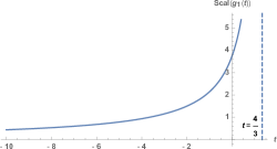
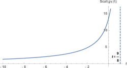
Figure 1. The graph of $\operatorname{\mathsf{Scal}}(g_{1}(t))$ for $\operatorname{\mathsf{G}}_{2}/\operatorname{\mathsf{U}}(2)$ (left) and $\operatorname{F}_{4}/\operatorname{\mathsf{Sp}}(3)\times\operatorname{\mathsf{U}}(1)$ (right).

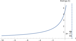
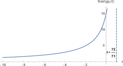
Figure 2. The graph of $\operatorname{\mathsf{Scal}}(g_{2}(t))$ for $\operatorname{\mathsf{G}}_{2}/\operatorname{\mathsf{U}}(2)$ (left) and $\operatorname{F}_{4}/\operatorname{\mathsf{Sp}}(3)\times\operatorname{\mathsf{U}}(1)$ (right).

The graphs now of the ricci components of the solutions $g_{j}(t)$,which we denote by

$$\operatorname{\mathsf{ric}}_{ij}(t):=\operatorname{\mathsf{ric}}_{i}(g_{j}(t))\,,\quad 1\leq i\leq r\,,\quad 1\leq j\leq N,$$

where again $N$ represents the number of fixed points of HRF at infinity of $\operatorname{\mathscr{M}}^{G}$, are very similar. For example, for any flag manifold $M=G/K$ with $r=2$ and for the first ancient solution $g_{1}(t)$ passing through the invariant Kähler-Einstein metric $g_{1}(0)=g_{KE}$, we compute

$$\operatorname{\mathsf{ric}}_{11}(t)=\operatorname{\mathsf{ric}}_{1}(g_{1}(t))=\operatorname{\mathsf{ric}}_{21}(t)=\operatorname{\mathsf{ric}}_{2}(g_{1}(t))=\frac{d_{1}+2d_{2}}{2(d_{1}+4d_{2})-2(d_{1}+2d_{2})t}\,.$$

For the solution $g_{2}(t)$ passing from the non-Kähler invariant Einstein metric $g_{2}(0)=g_{E}$ we obtain

$$\operatorname{\mathsf{ric}}_{12}(t)=\operatorname{\mathsf{ric}}_{1}(g_{2}(t))=\operatorname{\mathsf{ric}}_{22}(t)=\operatorname{\mathsf{ric}}_{2}(g_{2}(t))=\frac{d_{1}^{2}+6d_{1}d_{2}+4d_{2}^{2}}{2(d_{1}^{2}+6d_{1}d_{2}+8d_{2}^{2})-2(4d_{2}^{2}+d_{1}^{2}+6d_{1}d_{2})t}\,.$$

Note that the equalities $\operatorname{\mathsf{ric}}_{11}(t)=\operatorname{\mathsf{ric}}_{21}(t)$ and $\operatorname{\mathsf{ric}}_{12}(t)=\operatorname{\mathsf{ric}}_{22}(t)$ occur since $g_{i}(t)$ $(i=1,2)$ are both 1-parameter families of invariant Einstein metrics on $M=G/K$ (as we mentioned in Section 2). For instance, for $\operatorname{\mathsf{G}}_{2}/\operatorname{\mathsf{U}}_{2}$ with $r=2$, the above formulas reduce to

$$\operatorname{\mathsf{ric}}_{11}(t)=\operatorname{\mathsf{ric}}_{21}(t)=\frac{12}{32-24t}\,,\quad\operatorname{\mathsf{ric}}_{12}(t)=\operatorname{\mathsf{ric}}_{22}(t)=\frac{88}{192-176t}\,,$$

with $\operatorname{\mathsf{ric}}_{11}(0)=\operatorname{\mathsf{ric}}_{21}(0)=\lambda_{1}=3/8$ and $\operatorname{\mathsf{ric}}_{12}(0)=\operatorname{\mathsf{ric}}_{22}(0)=\lambda_{2}=11/24$, respectively. The corresponding graphs are given in Figure 3.

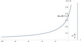
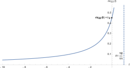
Figure 3. The graphs of $\operatorname{\mathsf{ric}}_{11}(t)=\operatorname{\mathsf{ric}}_{21}(t)$ and $\operatorname{\mathsf{ric}}_{12}(t)=\operatorname{\mathsf{ric}}_{22}(t)$ for $\operatorname{\mathsf{G}}_{2}/\operatorname{\mathsf{U}}(2)$ with $\mathfrak{m}=\mathfrak{m}_{1}\oplus\mathfrak{m}_{2}$.

Example 3.4.

Let $M=G/K$ be a flag manifold with $b_{2}(M)=1$ and $r=3$. Let us describe the asymptotic properties of the scalar curvature $\operatorname{\mathsf{Scal}}(g_{1}(t))$, related to the solution $g_{1}(t)=(1-2\lambda_{1}t)\cdot\mathfrak{e}_{1}$ only, where $\mathfrak{e}_{1}=(1,2,3)$ is the fixed point corresponding to the invariant Kähler-Einstein metric $g_{1}(0)\equiv g_{KE}$. By (3.3) we see that $\operatorname{\mathsf{Scal}}(g_{1}(t))$ is the positive hyperbola given by

$$\operatorname{\mathsf{Scal}}(g_{1}(t))=\frac{(d_{1}+d_{2}+d_{3})(d_{1}+2d_{2}+3d_{3})}{2(d_{1}+4d_{2}+9d_{3})+2t(d_{1}+4d_{2}+6d_{3})}\,.$$

Thus, $\operatorname{\mathsf{Scal}}(g_{1}(t))$ increases on the open interval $(-\infty,\frac{1}{2\lambda_{1}})$, where $g_{1}(t)$ is dedined. Note that the value $\operatorname{\mathsf{Scal}}(g(0))=\frac{(d_{1}+d_{2}+d_{3})(d_{1}+2d_{2}+3d_{3})}{2(d_{1}+4d_{2}+9d_{3})}$ equals to the scalar curvature of the Kähler-Einstein metric $g_{1}(0)$. The limit of $\operatorname{\mathsf{Scal}}(g_{1}(t))$ as $t\to\frac{1}{2\lambda_{1}}$ must be considered only from below, and it follows that

$$\lim_{t\to\frac{1}{2\lambda_{1}}}\operatorname{\mathsf{Scal}}(g_{1}(t))=+\infty\,,\quad\lim_{t\to-\infty}\operatorname{\mathsf{Scal}}(g_{1}(t))=0\,.$$

For example for $\operatorname{\mathsf{G}}_{2}/\operatorname{\mathsf{U}}_{2}$ and $r=3$, we compute $\lambda_{1}=5/24$, so

$$\operatorname{\mathsf{Scal}}(g_{1}(t))=\frac{25}{12-5t}\,,\quad t\in(-\infty,\frac{12}{5})\,,\quad\operatorname{\mathsf{Scal}}(g_{1}(0))=\frac{25}{12}$$

and the graph of $\operatorname{\mathsf{Scal}}(g_{1}(t))$ is given by

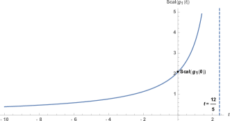
Figure 4. The graph of $\operatorname{\mathsf{Scal}}(g_{1}(t))$ for $\operatorname{\mathsf{G}}_{2}/\operatorname{\mathsf{U}}(2)$ with $\mathfrak{m}=\mathfrak{m}_{1}\oplus\mathfrak{m}_{2}\oplus\mathfrak{m}_{3}$.

References

• [AbN16] Abiev, N. A., and Yu.G. Nikonorov. “The evolution of positively curved invariant Riemannian metrics on the Wallach spaces under the Ricci flow.” Ann. Glob. Anal. Geom., 50 (1), (2016), 65–84.
• [A$\ell$C19] Alekseevksy, D.V., and I. Chrysikos. “Spin structures on compact homogeneous pseudo-Riemannian manifolds.” Transformation Groups, 24 (3), (2019), 659–689.
• [A$\ell$K75] Alekseevsky, D.V., and B. N. Kimel’fel’d. “Structure of homogeneous Riemannian spaces with zero Ricci curvature.” Functional Analysis and its Applications 9, (2) (1975), 5–11.
• [A$\ell$P86] Alekseevsky, D.V., and A. Perelomov. “Invariant Kähler-Einstein metrics on compact homogeneous spaces.” Functional Analysis Applications 20, no. 3 (1986): 171–182.
• [A$\ell$VL91] Alekseevsky, D.V., Vinogradov, A. M., and V. V. Lychagin. “Geometry I - Basic Ideas and Concepts of Differential Geometry.” Encyclopaedia of Mathematical Sciences,Vol. 28, Springer-Verlag, Berlin, 1991.
• [AB15] Alexandrino, M., and R. G. Bettiol. “Lie Groups and Geometric Aspects of Isometric Actions.” Springer International Publishing, Switzerland 2015.
• [AnC11] Anastassiou, S., and I. Chrysikos. “The Ricci flow approach to homogeneous Einstein metrics on flag manifolds.” Journal of Geometry and Physics 61, (2011): 1587–1600.
• [AC10] Arvanitoyeorgos, A., and I. Chrysikos. “Invariant Einstein metrics on generalized flag manifolds with four isotropy summands.” Ann. Glob. Anal. Geom., 37, no 2 (2010): 185–219.
• [AC11] Arvanitoyeorgos, A., and I. Chrysikos. “Invariant Einstein metrics on generalized flag manifolds with two isotropy summands.” J. Austral. Math. Soc., 90 (02), (2011), 237–251.
• [Bö04] Böhm, C. “Homogeneous Einstein metrics and simplicial complexes.” J. Differential Geom., 67 (1), (2004), 79–165.
• [Bö15] Böhm, C. “On the long time behavior of homogeneous Ricci flows.” Comment. Math. Helv., 90 (2015), 543–571.
• [BöL18a] Böhm, C., and R. A. Lafuente. “Immortal homogeneous Ricci flows.” Invent. math. 212, (2018), 461–529.
• [BöLS17] Böhm, C., Lafuente, R. A., and M. Simon. “Optimal curvature estimates for homogeneous Ricci flows.” Intern. Math. Res. Not., 00 (2017), 1–38.
• [BöL18b] Böhm, C., and R. A. Lafuente. “Homogeneous Einstein metrics on Euclidean spaces are Einstein solvmanifolds.” arXiv:1811.12594
• [BöWZ04] Böhm, C., Wang, M., and W. Ziller. “A variational approach for homogeneous Einstein metrics.” Geom. Funct. Anal., 14 (4) (2004), 681-733.
• [BöW07] Böhm, C., and B. Wilking. “Nonnegatively curved manifolds with finite fundamental groups admits metrics with positive Ricci curvature.” Geom. Funct. Anal., 17 (2007), 665–681.
• [BH58] Borel, A., and F. Hirzebruch. “Characteristics classes and homogeneous spaces I.” Amer. J. Math., 80 (1958), 458–538.
• [Buz14] M. Buzano, Ricci flow on homogeneous spaces with two isotropy summands, Ann. Glob. Anal. Geom. 45 (2014), 25–45.
• [CE75] Cheeger, J., and D. G. Ebin. “Comparison Theorems in Riemannian Geometry.” North-Holland Publishing Company, 1975.
• [Ch09] Chen, B-L. “Strong uniqueness of the Ricci flow.” J. Differential Geom., 82 (2), (2009), 363–382.
• [ChZ06] Chen, B.-L., and Zhu, X.-P. “Uniqueness of the Ricci flow on complete non-compact Riemannian manifolds.” J. Diff. Geom., 74, (2006), 119–154.
• [CLN06] Chow, B., Lu, P., and L. Ni: “Hamilton’s Ricci Flow.” Amer. Math. Soc. 2006.
• [C12] Chrysikos, I. “Flag manifolds, symmetric $\mathfrak{t}$-triples and Einstein metrics.” Differential Geometry and its Applications 30, (2012): 642–659.
• [CS14] Chrysikos, I., and Y. Sakane. “The classification of homogeneous Einstein metrics on flag manifolds with $b_{2}(M)=1$.” Bulletin Sciences Mathématiques, 138, (2014): 665–692.
• [EMT11] Enders, J., Müller, R., and P. Topping. “On type-I singularities in Ricci flow.” Comm. Anal. Geom., 19 (5), (2011), 905–922.
• [Fu$\ell$93] Fulton, W. “Introduction to Toric Varieties.” Princeton University Press, Princeton New Jersey 1993
• [G69] Gonzales. E. A. V. “Generic properties of polynomial vector fields at infinity.” Trans. Amer. Math. Soc., 143 (1969), 201–222.
• [GM09] Grama, L., and R. M. Martins. “The Ricci flow of left invariant metrics on full flag manifold $SU(3)/T$ from a dynamical systems point of view.” Bull. Sci. Math., 133 (2009): 463–469.
• [GM12] Grama, L., and R. M. Martins. “Global behavior of the Ricci flow on generalized flag manifolds with two isotropy summands.” Indagationes Mathematicae, 23 (1-2), (2012): 95–104.
• [GMPSS20] Grama, L., Martins, R. M., Patrão, M., Seco, L., and L. D. Sperança. “Global dynamics of the Ricci flow on flag manifolds with three isotropy summands.” arXiv:2004.01511
• [Gr06] Graev, M. “On the number of invariant Eistein metrics on a compact homogeneous space, Newton polytopes and contraction of Lie algebras.” International Journal of Geometric Methods in Modern Physics 3, no. 5-6 (2006): 1047–1075.
• [Gr13] Graev, M. “On the compactness of the set of invariant Einstein metrics” Ann. Glob. An. Geom., (44), (2013), 471–500.
• [H82] Hamilton, R. “Three-manifolds with positive Ricci curvature.” J.Diff. Geom., 17 (1982) 255-306.
• [Ker98] Kerr, M. “New examples of of homogeneous Einstein metrics.” Michigan J. Math., 45, (1998), 115–134.
• [Kim90] Kimura, M. “Homogeneous Einstein metrics on certain Kähler C-spaces.” Adv. Stud. Pure. Math., 18-I (1990), 303–320.
• [KN69] Kobayashi, S., and K. Nomizu. ’Foundations of Differential Geometry Vol II.” Wiley - Interscience, New York, 1969.
• [Kot10] Kotschwar, B. “Backwards uniqueness for the Ricci flow.” Int. Math. Res. Not., IMRN 21 (2010), 4064–97.
• [Laf15] Lafuente, R. A. “Scalar curvature behavior of homogeneous Ricci flows.” J. Geom. Anal., 25, (2015), 2313–2322.
• [LL14a] Lafuente, R., and J. Lauret. “On homogeneous Ricci solitons.” Quart. J. Math., 65 (2), (2014), 399–419
• [LL14b] Lafuente, R., and J. Lauret. “Structure of homogeneous Ricci solitons and the Alekseevskii conjecture.” J. Differential Geom., 98 (2), (2014), 315–347.
• [L11a] Lauret, J. “The Ricci flow for simply connected nilmanifolds.” Commun. Anal. Geom.,19 (5), (2011), 831–854.
• [L11b] Lauret, J. “Ricci soliton solvmanifolds.” J. reine angew. Math., 650 (2011), 1–21.
• [L13] Lauret, J. “Ricci flow of homogeneous manifolds.” Math. Zeitschrift, 274, (2013), 373–403.
• [LW17] Lu, P., and Y. K. Wang. “Ancient solutions of the Ricci flow on bundles.” Adv. Math., 318, (2017), 411–456.
• [NRS07] Nikonorov, Yu. G., Rodionov, E. D., and V. V. Slavskii. “Geometry of homogeneous Riemannian manifolds.” J. Math. Sci., 146, (6), (2007), 6313–6390.
• [PS97] Park, J-S., and Y. Sakane. “Invariant Einstein metrics on certain homogeneous spaces.” Tokyo J. Math., 20 (1) (1997), 51–61.
• [Pn10] Payne, T. L. “The Ricci flow for nilmanifolds.” J. Modern Dynamics, 4 (1), (2010), 65–90.
• [P02] Perelman, G. “The entropy formula for the Ricci flow and its geometric applications.” arXiv:math/0211159.
• [P03] Perelman, G. “Ricci flow with surgery on three-manifolds.” arXiv:math/0303109v1.
• [PP15] Panelli, F., and F. Podestà. “On the first eigenvalue of invariant Kähler metrics.” Math. Z., 281, (2015), 471–482.
• [P1891] Poincaré, H. “Sur l’ integration des équations différentielles du premier ordre et du premier degré I.” Rendiconti del circolo matematico di Palermo, 5, (1891), 161–191.
• [PR19] Pulemotov, A., and Y. A. Rubinstein. “Ricci iteration on homogeneous spaces.” Trans. Amer. Math. Soc., 371, (2019), 6257–6287.
• [S99] Sakane, Y. “Homogeneous Einstein metrics on flag manifolds.” Lobachevskii J. Math, 4, (1999), 71–87.
• [VG03] Vidal, C., and P. Gomez. “An extension of the Poincare compactification and a geometric interpretation.” Proyecciones J. Math., 22 (3), (2003), 161–180.
• [WZ86] Wang, M., and W. Ziller. “Existence and non-excistence of homogeneous Einstein metrics.” Invent. Math., 84 (1986), 177–194.