A variational asymmetric phase-field model of quasi-brittle fracture:
Energetic solutions and their computation.

Abstract

We derive the variational formulation of a gradient damage model by applying the energetic formulation of rate-independent processes and obtain a regularized formulation of fracture. The model exhibits different behaviour at traction and compression and has a state-dependent dissipation potential which induces a path-independent work. We will show how such formulation provides the natural framework for setting up a consistent numerical scheme with the underlying variational structure and for the derivation of additional necessary conditions of global optimality in the form of a two-sided energetic inequality. These conditions will form our criteria for making a better choice of the starting guess in the application of the alternating minimization scheme to describe crack propagation as quasistatic evolution of global minimizers of the underlying incremental functional. We will apply the procedure for two- and three-dimensional benchmark problems and we will compare the results with the solution of the weak form of the Euler-Lagrange equations. We will observe that by including the two-sided energetic inequality in our solution method, we describe, for some of the benchmark problems, an equilibrium path when damage starts to manifest, which is different from the one obtained by solving simply the stationariety conditions of the underlying functional.

Keywords:Phase field variable. Generalized standard material. Energetic formulation. Two sided energetic inequality. Alternating minimization. Backtracking algorithm.

^∗ Corresponding author.
Email: {mluege, aorlando}@herrera.unt.edu.ar

1 Introduction

In computational fracture mechanics, the variational phase-field models of fracture have received a considerable and increased attention as approximation models of fracture since the seminal works [34, 17] where the classical concept of Griffith’s critical energy release rate [44] is replaced by a least energy principle, making it possible to capture otherwise characteristic features of the fracture process. These models of fracture can appear as regularization formulations of free-discontinuity problems in the context of the variational approach to fracture [34, 23, 35, 27, 42], or they can result from the modelling of gradient damage as application of material constitutive theories in terms of two potentials, the free energy density and the dissipation potential [36, 38, 54, 55, 7, 61, 62, 63]. Excellent reviews on the application of these two approaches to approximate quasi-brittle fracture according to the above sense can be found in [5, 14, 72, 80, 30] whereas [31, 29, 83, 84] provide an extensive overview of also other phase-field models, not only the variational ones, that have been lately proposed for providing a more accurate description of the fracture process. In the variational formulations the cracks are represented by a continuum variable, namely a phase-field variable, that can be identified with the damage variable $\beta$ which describes the damaged and the undamaged phases, whereas their propagation is described by the quasistatic evolution of the critical points of an energetic functional which accounts for the stored elastic energy and the dissipation associated with the variation of $\beta$. The main advantages of these formulations, compared for instance to the discrete approaches to fracture [67], which relies on explicit modelling of the displacement field discontinuity jump produced by the crack, is that phase-field formulations can handle the evolution of complex crack patterns, can account for crack initiation and propagation without initial defects and prescribed crack path, and can be implemented without any particular consideration of what the crack pattern will be. This is because one deals with the search for critical points of functionals defined over Sobolev spaces which can be easily discretized by standard finite elements spaces [74] and crack initiation and propagation appear as a result of a competition between the different energetic terms [78].

The existence of a variational structure for the models which we consider in this paper is basically a consequence of the rate-independence and associativity of the evolution process, thus the need to work with standard damage models [59, 69, 12]. In this case, the variational formulation can be derived quite naturally by a general theoretical framework of clear mechanical interpretation given by the energetic formulation proposed by Mielke and coworkers [65, 66]. The use of the energetic formulation indirectly defines also the type of critical point which must be considered for the description of the evolution process. Since the existence of energetic solutions is proved by considering the evolution along global minimizers of discrete functionals, which are those that we use in the numerical simulation, the concept of global minimizer is therefore the appropriate critical point we will use in this paper. This modelling assumption, which represents a milestone of the variational approach of fracture advanced in [34], has been analysed and justified theoretically, for instance, in [27, 16, 33, 42, 61, 58], though the evolution via global minimzation is also subject of debate because it is not always able to produce physical solutions [20, 77, 1]. For instance, in [1] it is shown that by applying the energetic formulation, the evolution along global minimizers could produce early and unphysical discontinuity jumps, thus the relevance of an evolution along other type of critical points is also beeing investigated as in [28, 4, 1, 19] to the fraction of cost of adding further physical based conditions about the choice of the particular critical point or of a redefinition of the concept of evolution as in [4, 1].

From the numerical standpoint, the computation of global minimizers of the discrete energetic functional, which is separately convex in the displacement field $\bm{u}$ and in the phase-field damage variable $\beta$, poses the problem to ensure the global optimality of the critical points that one computes. The application of brute-force global optimization algorithms, such as clustering like or stocastic methods does not represent, at the moment, a viable option. In practice, one considers the Euler-Lagrange equations of this minimizing principle, and then apply the finite element method to their weak formulations [62, 63, 39, 40, 81, 84] or apply an alternating minimization method (referred to also as staggered scheme) to the finite element discrete energetic functional [21, 32, 80]. However, this methodology contrasts with the underlying modelling assumption of global minimization. Since the functional is non-convex, the Euler-Lagrange equations represent only stationariety conditions, thus their satisfaction cannot guarantee the global optimality of the computed solution. Same conclusion holds by applying the staggered procedure given that the sequence of iterates, eventually up to a subsequence, converges to a critical point of the discrete energetic functional [4, 50]. Notably exceptions to this approach are those methods where the search of a global minimizer is realized still by local optimization algorithms which are however augmented by conditions met by the global minimizers [66, 15, 25, 60]. On the basis of these additional necessary conditions of global optimality, one basically tries to make a better choice of the starting guess so that it falls within the attraction basin of a global minimizer. This procedure has been applied successfully to the simulation of isotropic damage in [15] and [66] by the variational and energetic formulation, respectively; to the simulation of the energetic formulation of a delamination and adhesive contact model in [76, 85] and to the simulation of hysteresis in magnetic shape memory composites by the energetic formulation in [25]. A similar idea, though applied in a different context, has been used in [22] to obtain fast and efficient numerical relaxation algorithms for the simulation of microstructures in single crystals with one active slip system. Here the authors exploit the structure of the modelling problem to obtain a better starting guess for the minimization of the nonconvex functional that models the problem at hand.

In this paper, starting from the mechanical model of [7, 63], we illustrate the complete procedure for the derivation of the corresponding energetic formulation, of the additional optimality conditions of the discrete energetic solutions in the form of a two-sided energy inequality, and the ensuing energy-balance-based backtracking strategy for the numerical simulation of the phase-field damage model, characterized by a different behaviour between traction and compression and with a state-dependent dissipation potential which induces a path-independent dissipated work. The discrete energetic functional we obtain is the same as the regularized functional considered in [23] which is usually known as AT2-model in the literature on the regularized formulations of fracture [7, 59, 30] and has been shown in [23] to $\Gamma-$converge (in the appropriate topology) to the free-discontinuity functional of [34] with the additional non-interpenetration constraint of the crack faces under compression. The term AT stands for Ambrosio-Torterelli who were the first to propose an elliptic regularization of the Mumford-Shah free-discontinuity functional [6]. To ensure that the discrete energetic solutions meet the additional conditions of globality, and to develop in this manner a computational strategy consistent with the modelling paradigma of evolution along global minimizers, we apply the strategy of backtracking in the context of an alternating minimization of the separately convex discrete energetic functional. By such algorithm adapted to rate-independent processes [10], we go back over the time steps, whenever the two-sided-energy inequality is violated at the current time, to restart the simulation with a different initial guess which is built on the basis of the computed states that violate the check test given by the energetic bounds. By comparing our simulations to those based on the solution of the weak form of the Euler-Lagrange equations, we observe that for some of our benchmark problems the energetic solutions describe an equilibrium path that deviates from the standard one when damages starts to manifest, though eventually the two paths coincide. The two-sided energy inequality does not only represent a quick test of whether the candidate solution can be completed to a valid solution, but it has also a relevant physical meaning. This condition in fact represents a discrete equivalent of the conservation of energy [66, 65]. Compared to [66], the present work enlarges the field of applications to state dependent dissipation potentials and to phase-field models that account for the non-interpenetration condition when they are considered as fracture approximation models. It also proposes a numerical procedure which is consistent with the underlying globality assumption of the model by exploiting properties of the global minimizers.

After this brief introduction, in the next Section we derive the phase-field model of fracture introduced in [7, 63] by applying the constitutive material theory based on the extended virtual power developed in [36]. We will introduce therefore the additive decomposition of the free elastic energy $\psi_{0}$ into a ‘compressive’ and ‘tensile’, with only the tensile contribution degraded by damage development. We use such decomposition to enforce in the limit the non–interpenetration condition in view of the $\Gamma-$convergence result of [23], though the assumption of the decomposition of the free energy for the formulation of regularized variational formulations of fracture that accounts for the non–interpenetration constraint has been debated, for instance, in [51, 35]. At this stage, we do not go into the specific of such decomposition which is not relevant for the subsequent theoretical developments, though, when we consider the actual implementation of the model, we will then refer to the decomposition of $\psi_{0}$ that results from the spectral splitting of the strain $\bm{\varepsilon}$ proposed in [63]. The objective of Section 2 is to relate the mechanical model as is given in the literature to the energetic formulation which is the subject of Section 3. In this Section, we give first the continuous formulation which describes the evolution in time of the rate-independent system, and then we present the discrete energetic functional as approximation of the continuous energetic formulation. We will also mention therein the relation between this approach and the ones in the literature [38, 54, 56, 70, 57], and derive the important energetic bounds of the discrete energetic solution by exploiting the property of global optimality. Section 4 describes then the alternating minimization algorithm. The corresponding finite element discrete equations and how the energetic based backtracking algorithm is used in the whole numerical strategy is explained in Section 5 whereas Section 6 gives applications of the full procedure to the numerical solution of $2d-$ and $3d-$benchmark problems. The results are compared to the numerical solutions obtained without the activation of the backtracking algorithm, that is, the solution of the weak form of the Euler-Langrange equations of the discrete energetic functional. Section 7 concludes the paper with some final remarks about the energetic formulation and the proposed procedure.

2 Mechanical derivation of the phase-field model of fracture

In this section we derive the phase-field model of fracture introduced in [7, 63] by applying the constitutive material theory developed in [36].

2.1 Notations, main assumptions and field equations

Let $\Omega\subset\mathbb{R}^{n}$, $n=1,2,3$, be a bounded open domain which we take as reference configuration of an homogeneous body made of brittle damaging material. We denote by $\partial\Omega$ the boundary of the domain $\Omega$, and assume that $\partial\Omega$ is split into two parts: a Dirichlet boundary $\partial\Omega_{D}$ and the remaining Neumann boundary $\partial\Omega_{N}:=\partial\Omega\setminus\partial\Omega_{D}$ where displacements $\bm{w}$ and surface tractions $\bm{t}$ are prescribed, respectively. The boundary $\partial\Omega$ is such that the outward normal $\bm{n}$ can be defined almost everywhere (a.e.) on $\partial\Omega$. We assume the displacement field $\bm{u}$ to be small and the system to undergo an isothermal quasi-static evolution over the time interval of interest $[0,\,T]$, $T>0$ and with uniform temperature in $\Omega$. The state of the system is then characterized by the linearized strain $\bm{\varepsilon}(\bm{u})=\nabla_{s}\bm{u}:=(\nabla\bm{u}+\nabla\bm{u}^{T})/2$, where $\nabla$ denotes the gradient operator, and additional variables which are introduced to capture the effects of microfractures at the material point on its macroscopic properties. As such additional variables we consider the damage variable field $\beta$ and its gradient $\nabla\beta$. The field variable $\beta$ can take values in $[0,\,1]$ with $\beta=0$ when the material is undamaged and $\beta=1$ for completed damaged material, i.e. when the material is not able to sustain any stress. Its gradient $\nabla\beta$ is introduced to account for the influence of the damage at a point on damage of its neighborhood. Following the method of virtual power, we assume as in Frémond [36, 37] that damage is produced by microscopic motions which break bonds among particles and such motion is described on the macroscopic level by the rate quantities $\dot{\beta}:=d\beta/\operatorname{\mathrm{d}\mathit{t}}$ and $\nabla\dot{\beta}:=\nabla(d\beta/\operatorname{\mathrm{d}\mathit{t}})$. The underlying assumption of the theory is that the power of these motions must be taken into account in the power of the internal forces. For background on continuum mechanics and corresponding notation, we refer to [45, 36].

To define the functional setting where to formulate our model, we introduce the standard Sobolev spaces $W^{1,\infty}(\Omega;\,\mathbb{R}^{n})$ and $H^{1}(\Omega;\,\mathbb{R}^{n})$ of functions defined a.e. in $\Omega$ and with values in $\mathbb{R}^{n}$, $n=1,2,3$. We denote then by $\mathcal{V}\subset H^{1}(\Omega;\,\mathbb{R}^{n})$ the space of all displacement fields that generate compatible strain fields, by $\mathcal{V}_{D}\subset\mathcal{V}$ the affine space of kinematically admissible fields, i.e. for any $t\in[0,\,T]$, $\bm{u}(\cdot,t)\in\mathcal{V}$ such that $\bm{u}=\bm{w}$ on $\partial\Omega_{D}$ in the sense of trace, and by $\mathcal{V}_{D,0}\subset\mathcal{V}$ the linear space of the kinematically admissible virtual displacement fields, that is, the space of the displacement fields $\bm{u}_{D,0}$ meeting the homogeneous kinematic boundary conditions on $\partial\Omega_{D}$, i.e. $\bm{u}_{D,0}=\bm{0}$ on $\partial\Omega_{D}$. We then introduce the linear space of the damage fields $\mathcal{B}=\{\gamma\in W^{1,\infty}(\Omega;\,\mathbb{R}):\,\nabla\gamma\cdot\bm{n}=0\text{ on }\partial\Omega\}$ and consider $\beta\in W^{1,1}([0,\,T];\,\mathcal{B})$ as function of $t$, [65, page 120].

For any $t\in[0,\,T]$, let $\bm{u}_{D,\bm{w}}(\cdot,t)\in\mathcal{V}_{D}$ be a lifting of the Dirichlet boundary data $\bm{w}(\cdot,t)$ [74], that is, $\bm{u}_{D,\bm{w}}(\cdot,t)$ is a given (fixed) extension of $\bm{w}(\cdot,t)$ onto $\overline{\Omega}$, the closure of $\Omega$ with $\overline{\Omega}=\Omega\cup\partial\Omega_{D}\cup\partial\Omega_{N}$. Such extension can be obtained, for instance, by taking an interpolation of $\bm{w}$ onto $\overline{\Omega}$ by finite element shape functions and must be considered as a known function once $\bm{w}(\bm{x},t)$ is given. We use also the notation $\bm{\varepsilon}_{D,0}=\nabla_{s}\bm{u}_{D,0}$ to refer to the linearized strain of virtual admissible displacement fields.

The internal virtual power is then defined by the linear form

$$\mathcal{P}_{i}(\dot{}\bm{u}_{D,0},\,\dot{\beta})=\int_{\Omega}\left(\bm{\sigma}\colon\dot{}\bm{\varepsilon}_{D,0}+V\dot{\beta}+\bm{H}\cdot\nabla\dot{\beta}\right)\,\operatorname{\mathrm{d}\bm{\mathit{x}}}$$

which defines the field variables $\bm{\sigma}$, $V$ and $\bm{H}$ dual of $\dot{}\bm{\varepsilon}$, $\dot{\beta}$ and $\nabla\dot{\beta}$, respectively. In this paper only volume forces $\bm{f}$, surface tractions $\bm{t}$ on $\partial\Omega_{N}$ and prescribed displacements $\bm{w}$ on $\partial\Omega_{D}$ are accounted for producing damage, thus the external virtual power is represented by the linear form

$$\mathcal{P}_{e}(\dot{}\bm{u}_{D,0})=\int_{\Omega}\bm{f}\cdot\dot{}\bm{u}_{D,0}\,\operatorname{\mathrm{d}\bm{\mathit{x}}}+\int_{\partial\Omega_{N}}\bm{t}\cdot\dot{}\bm{u}_{D,0}\,dx\,.$$

The principle of the virtual power then states

$$\mathcal{P}_{e}(\dot{}\bm{u}_{D,0})=\mathcal{P}_{i}(\dot{}\bm{u}_{D,0},\,\dot{\beta})$$

which must hold for any admissible $\dot{}\bm{u}_{D,0}\in\mathcal{V}_{D,0}$ and $\dot{\beta}\in\mathcal{B}$. By applying the Gauss-Green theorem and then the fundamental lemma of the calculus of variations, we obtain two field equations, one is the balance equations of linear momentum

$$\begin{array}[]{ll}\displaystyle\operatorname{\mathsf{div}}\bm{\sigma}+\bm{f}=\bm{0}&\text{ in }\Omega\\ \displaystyle\bm{\sigma}\bm{n}=\bm{t}&\text{ on }\partial\Omega_{N}\end{array}$$ (2.1)

with the corresponding Neumann boundary condition given by the Cauchy Theorem [45], whereas the other is the microforce balance equations

$$\begin{array}[]{ll}\displaystyle\operatorname{\mathsf{div}}\bm{H}-V=0&\text{ in }\Omega\\ \displaystyle\bm{H}\cdot\bm{n}=0&\text{ on }\partial\Omega\end{array}$$ (2.2)

with the corresponding boundary value.

2.2 The differential constitutive model

We consider the coupled elasto–damage model defined by the following potentials

$$\displaystyle\psi(\bm{\varepsilon},\,\beta,\,\nabla\beta)=\displaystyle R(\beta)\psi_{0}^{+}(\bm{\varepsilon})+\psi_{0}^{-}(\bm{\varepsilon})+\displaystyle\frac{g_{c}\ell}{2}|\nabla\beta|^{2}+I_{[0,\,1]}(\beta)\,,$$ (2.3a)

$$\displaystyle\phi(\dot{\beta};\,\beta)=\frac{g_{c}}{\ell}\beta\dot{\beta}+I_{\mathbb{R}^{+}}(\dot{\beta})\,,$$ (2.3b)

where $I_{\mathbb{A}}$ is the indicator function of the set $\mathbb{A}$ and is defined by $I_{\mathbb{A}}(x)=0$ if $x\in\mathbb{A}$ and $I_{\mathbb{A}}(x)=+\infty$ if $x\not\in\mathbb{A}$. We use the notation $\mathbb{R}^{+}=\{x\in\mathbb{R}:x\geq 0\}$ and denote by $R(\beta)=g(\beta)+k$ the degradation function where $g(\beta)$ is decreasing with $\beta$, convex and Lipschitz and such that $g(0)=1$ and $g(\beta)=1$ whereas $k$ is a small positive parameter that precludes complete damage by ensuring an artificial residual stiffness of a totally broken phase when $\beta=1$. The symbol $g_{c}$ is the fracture toughness whereas $\ell>0$ has the dimension of a length and controls the width of the transition zone of $\beta$. Such parameter identifies with the regularization parameter in the variational model of fracture. Finally $\psi_{0}^{+}$ and $\psi_{0}^{-}$ are the ‘tensile’ and ‘compressive’ parts of the elastic strain energy density $\psi_{0}$ which can be derived, for instance, from the so-called volumetric-deviatoric splitting of the strain tensor $\bm{\varepsilon}$ [7, 35, 51] or the spectral decomposition of $\bm{\varepsilon}$ [63, 62], though also other options for constructing $\psi_{0}^{+}$ and $\psi_{0}^{-}$ have been suggested in [53, 71]. By (2.3a), it is assumed that only the positive part of the energy is degraded by the occurrence of damage, whereas the negative part remains unaffected by it.

We next show that this model is the same as the one proposed by [63, Eq. (61)] and [62, Eq. (38)] and corresponds to the AT2 regularized formulation of fracture of [16] apart from the presence of the splitting of the free elastic energy term [7, 59, 30].

Proposition 2.1.

The differential constitutive model defined by the potentials (2.3) is given by the state laws

$$\bm{\sigma}=\frac{\partial\psi}{\partial\bm{\varepsilon}}$$ (2.4)

and the following evolution laws

$$\left|\begin{array}[]{l}\displaystyle\dot{\beta}\geq 0\\[6.45831pt] \displaystyle-\frac{\partial\psi}{\partial\beta}-\frac{g_{c}}{\ell}(\beta-\ell^{2}\Delta\beta)\leq 0\\[6.45831pt] \displaystyle\dot{\beta}\Big{(}-\frac{\partial\psi}{\partial\beta}-\frac{g_{c}}{\ell}(\beta-\ell^{2}\Delta\beta)\Big{)}=0\,.\end{array}\right.$$ (2.5)

Proof.

We start from the Clausius-Duhem inequality for isothermal processes

$$\bm{\sigma}\colon\dot{}\bm{\varepsilon}+\bm{H}\cdot\nabla\dot{\beta}+V\dot{\beta}-\rho\dot{\psi}\geq 0\,,$$ (2.6)

and make the following constitutive assumptions

$$\bm{\sigma}=\bm{\sigma}^{nd}+\bm{\sigma}^{d}\,,\quad V=V^{nd}+V^{d}\quad\text{and}\quad\bm{H}=\bm{H}^{nd}+\bm{H}^{d}$$ (2.7)

which distinguish the components that are responsable of the dissipative and reversible mechanisms. By replacing (2.7) into (2.6) and by defining

$$\bm{\sigma}^{nd}=\frac{\partial\psi}{\partial\bm{\varepsilon}}\,,\quad V^{nd}=\frac{\partial\psi}{\partial\beta}\quad\text{and}\quad\bm{H}^{nd}=\frac{\partial\psi}{\partial(\nabla\beta)}$$ (2.8)

the Clausius-Duhem inequality reduces to the following expression

$$\bm{\sigma}^{d}\colon\dot{}\bm{\varepsilon}+V^{d}\dot{\beta}+\bm{H}^{d}\cdot\nabla\dot{\beta}\geq 0\,.$$ (2.9)

For our model we assume

$$\bm{\sigma}^{d}=\bm{0}\quad\text{and}\quad\bm{H}^{d}=\bm{0}\,,$$ (2.10)

thus (2.9) becomes

$$V^{d}\dot{\beta}\geq 0\,.$$ (2.11)

We can meet (2.11) by taking

$$V^{d}\in\partial_{\dot{\beta}}\phi(\dot{\beta};\,\beta)$$ (2.12)

given that the function (2.3b) is a dissipation potential. Now, by the constitutive assumptions (2.7) and (2.10), and given the expression (2.3a) of $\psi$, we have that

$$\bm{H}=\bm{H}^{nd}=g_{c}\ell\nabla\beta\,,$$

which replaced in (2.2), yields

$$V=\operatorname{\mathsf{div}}\bm{H}=g_{c}\ell\Delta\beta\,.$$

By accounting for the expression (2.8) of $V^{nd}$, we have thus

$$V^{d}=V-V^{nd}=g_{c}\ell\Delta\beta-\frac{\partial\psi}{\partial\beta}\,.$$ (2.13)

By computing $\partial_{\dot{\beta}}\phi$ we obtain

$$\partial_{\dot{\beta}}\phi(\dot{\beta};\,\beta)=\frac{g_{c}}{\ell}\beta+\partial_{\dot{\beta}}I_{\mathbb{R}^{+}}(\dot{\beta})\,,$$ (2.14)

thus (2.12) reads as

$$g_{c}\ell\Delta\beta-\frac{\partial\psi}{\partial\beta}-\frac{g_{c}}{\ell}\beta\in\partial_{\dot{\beta}}I_{\mathbb{R}^{+}}(\dot{\beta})\,,$$ (2.15)

where we have accounted for (2.13) and (2.14). By the definition of subdifferential of the indicator function [36, Appendix A.1.3], we have that (2.15) means

$$\begin{array}[]{ll}\displaystyle-\frac{\partial\psi}{\partial\beta}-\frac{g_{c}}{\ell}(\beta-\ell^{2}\Delta\beta)=0&\text{ if }\dot{\beta}>0\,,\\[6.45831pt] \displaystyle-\frac{\partial\psi}{\partial\beta}-\frac{g_{c}}{\ell}(\beta-\ell^{2}\Delta\beta)<0&\text{ if }\dot{\beta}=0\,,\\[6.45831pt] \displaystyle\varnothing&\text{ if }\dot{\beta}<0\,,\end{array}$$ (2.16)

which can then be expressed in the form given by (2.5). ∎

Remark 2.1.

The model defined by (2.4) and (2.5) is a generalized standard material in the meaning of [69, page 37] and [12, page 69] given that it can be defined by the two potentials, the free energy potential $\psi(\bm{\varepsilon},\,\beta,\,\nabla\beta)$ and the dissipation potential $\phi(\dot{\beta},\,\beta)$ using (2.7), (2.8), (2.10) and (2.12). Since for $\dot{\beta}\geq 0$, the dissipation potential $\phi$ is a gauge [46], the model is associative. The free energy and the dissipation potential are the only ingredients we need to set up the energetic formulation, henceforth to derive the incremental variational formulation. This will be shown in Section 3.2.

If in place of the dissipation potential (2.3b) we take [64, 66, 18, 78]

$$\phi(\dot{\beta})=\frac{g_{c}}{\ell}\kappa\dot{\beta}+I_{\mathbb{R}^{+}}(\dot{\beta})\,,$$ (2.17)

with $\kappa>0$ a phenomenological constant such that $\kappa g_{c}/\ell$ is an activation threshold that represents the specific energy dissipated by fully damaging the bulk material, then by the arguments of the proof of Proposition 2.1 we obtain the following evolution laws

$$\left|\begin{array}[]{l}\displaystyle\dot{\beta}\geq 0\\[6.45831pt] \displaystyle-\frac{\partial\psi}{\partial\beta}-\frac{g_{c}}{\ell}(\kappa-\ell^{2}\Delta\beta)\leq 0\\[6.45831pt] \displaystyle\dot{\beta}\Big{(}-\frac{\partial\psi}{\partial\beta}-\frac{g_{c}}{\ell}(\kappa-\ell^{2}\Delta\beta)\Big{)}=0\,.\end{array}\right.$$ (2.18)

We will see later in Remark 3.3$(ii)$ that the dissipation potential (2.17) defines the so-called AT1 regularized formulation of fracture [78]. Also, it is not difficult to verify that (2.18) leads to the existence of an elastic stage before onset of damage, that is, as long as $-\text{d}R(\beta)/\text{d}\beta\,\psi^{+}_{0}(\bm{\varepsilon})\leq\kappa g_{c}/\ell$, $\beta=0$ is solution of (2.18) whereas with the AT2 regularized formulation, as soon as $\psi_{0}^{+}(\bm{\varepsilon})\not=0$, the damage variable $\beta$ starts to evolve.

2.3 The incremental boundary value problem

Let $\mathcal{P}=\{0=t_{0}<t_{1},\,\ldots,\,t_{N}=T\},\,N\in\mathbb{N}$ be a discrete set of time instants that realize a partition of the time interval of interest $[0,\,T]$ and $\Delta t=\max_{n=0,1,\ldots,N-1}\{t_{n+1}-t_{n}\}$. Denote by $\bm{z}$ a kinematically admissible displacement field, that is, a displacement field that meets the Dirichlet boundary conditions at the current time $t$. Given $(\bm{z}_{n},\,\beta_{n})$ an approximation of the fields $\bm{z}$ and $\beta$ at the time instant $t_{n}$, we consider the incremental boundary value problem associated with the time step $[t_{n},\,t_{n+1}]$ obtained by an Euler implicit time discretization of the constitutive equations (2.4) and (2.5), and of the momentum balance equations (2.1) and (2.2). This problem consists of finding $(\bm{z}_{n+1},\,\beta_{n+1})$ such that the following relations are met

$$-\operatorname{\mathsf{div}}\bm{\sigma}_{n+1}-\bm{f}_{n+1}=\bm{0}\quad\text{in }\Omega\,,$$ (2.19a)

$$\bm{\varepsilon}_{n+1}=\nabla_{s}\bm{z}_{n+1},\quad\bm{\sigma}_{n+1}=\frac{\partial\psi}{\partial\bm{\varepsilon}}(\bm{\varepsilon}_{n+1},\beta_{n+1})\quad\text{in }\Omega\,,$$ (2.19b)

$$\bm{z}_{n+1}=\bm{u}_{D,n+1}\text{ on }\partial\Omega_{D}\,,\quad\bm{\sigma}_{n+1}\bm{n}=\bm{t}_{n+1}\text{ on }\partial\Omega_{N}\,,$$ (2.19c)

$$0\leq\beta_{n+1}\leq 1\quad\text{in }\Omega\,,$$ (2.19d)

$$\beta_{n+1}\geq\beta_{n}\quad\text{in }\Omega\,,$$ (2.19e)

$$-\frac{\partial\psi}{\partial\beta}(\bm{\varepsilon}_{n+1},\beta_{n+1})-\frac{g_{c}}{\ell}(\beta_{n+1}-\ell^{2}\Delta\beta_{n+1})\leq 0\quad\text{in }\Omega\,,$$ (2.19f)

$$(\beta_{n+1}-\beta_{n})\Big{(}-\frac{\partial\psi}{\partial\beta}(\bm{\varepsilon}_{n+1},\beta_{n+1})-\frac{g_{c}}{\ell}(\beta_{n+1}-\ell^{2}\Delta\beta_{n+1})\Big{)}=0\quad\text{in }\Omega\,,$$ (2.19g)

$$\nabla\beta_{n+1}\cdot\bm{n}=0\text{ on }\partial\Omega\quad\text{in }\Omega\,,$$ (2.19h)

where $\psi$ is given by (2.3a) without the indicator function $I_{[0,\,1]}(\beta)$ given that the constraint enforced by this function has been accounted explicitly by (2.19d). The condition (2.19e) is referred to as irreversibility condition and prevents material healing.

Remark 2.2.

For any given $\bm{\varepsilon}_{n+1}$, the model defined by (2.19e), (2.19f) and (2.19g) is similar to the one that describes the deformation of a membrane over a linear elastic obstacle represented by $\beta_{n}$ and loaded by $\partial\psi/\partial\beta$. For instance, using the classical assumption for $g(\beta)$ in $R(\beta)$ due to Kachanov [47], with $g(\beta)=1-\beta$, we have $\partial\psi/\partial\beta=-\psi_{0}^{+}(\bm{\varepsilon})$. For more general expressions of $R(\beta)$, such as the ones in [56, 57], $\partial\psi/\partial\beta$ has always a term that depends only on $\bm{\varepsilon}$ and another one that depends also on $\beta$. The latter would then modify the bilinear form associated with $\beta g_{c}/\ell-g_{c}\ell\Delta\beta$.

If we denote by $\mathbb{C}$ the convex set of admissible solutions for $\beta$

$$\mathbb{C}=\bigg{\{}\beta\in\mathcal{B}:\beta(x)\in[0,\,1]\text{ a.e. in }\Omega\text{ and }\beta\geq\beta_{n}\text{ a.e. in }\Omega\bigg{\}}\,,$$ (2.20)

and take $\bm{z}$ and $\beta$ as primary variables, we can consider the following weak formulation of (2.19):

$$\text{Find }(\bm{z}_{n+1},\,\beta_{n+1})\in\mathcal{V}_{D}\times\mathbb{C}:$$

$$\phantom{xxxxx}\int_{\Omega}\frac{\partial\psi}{\partial\bm{\varepsilon}}(\bm{\varepsilon}_{n+1},\,\beta_{n+1})\colon\bm{\varepsilon}(\bm{v})\,\operatorname{\mathrm{d}\bm{\mathit{x}}}=\int_{\Omega}\bm{f}\cdot\bm{v}\,\operatorname{\mathrm{d}\bm{\mathit{x}}}+\int_{\partial\Omega_{N}}\bm{t}\cdot\bm{v}\,\operatorname{\mathrm{d}\mathit{s}}\quad\text{for all }\bm{v}\in\mathcal{V}_{D,0}\,,$$ (2.21a)

$$\phantom{xxxxx}\int_{\Omega}\frac{\partial\psi}{\partial\beta}(\bm{\varepsilon}_{n+1},\beta_{n+1})(\gamma-\beta_{n+1})\,\operatorname{\mathrm{d}\bm{\mathit{x}}}+\int_{\Omega}\frac{g_{c}}{\ell}\beta_{n+1}(\gamma-\beta_{n+1})\,\operatorname{\mathrm{d}\bm{\mathit{x}}}$$

$$\phantom{xxxxxxxxxxxxxxxxxxxxxxxxxxx}+\int_{\Omega}g_{c}\ell\nabla\beta_{n+1}\nabla(\gamma-\beta_{n+1})\,\operatorname{\mathrm{d}\bm{\mathit{x}}}\geq 0\quad\text{for all }\gamma\in\mathbb{C}\,,$$ (2.21b)

where $\bm{\varepsilon}_{n+1}=\nabla_{s}\bm{z}_{n+1}$.

Remark 2.3.

Since $\psi$ is not convex, problem (2.21) is not ensured to have a unique solution. We will discuss this below with reference to the minimization formulation associated with (2.21).

This observation justifies therefore the following notion.

Definition 1.

We refer to any solution of (2.21) as a local solution of the model (2.3).

Proposition 2.2.

If $(\bm{z}_{n+1},\,\beta_{n+1})\in\mathcal{V}_{D}\times\mathbb{C}$ solves (2.21), then the field equations of (2.19) are met a.e. in $\Omega$ and the boundary conditions are met a.e. on the corresponding part of $\partial\Omega$.

Proof.

Let $(\bm{z}_{n+1},\,\beta_{n+1})\in\mathcal{V}_{D}\times\mathbb{C}$ be a solution of (2.21) and denote by $\mathcal{D}(\Omega)$ the space of the infinitely differentiable functions compactly supported in $\Omega$ i.e., for $\varphi\in\mathcal{D}(\Omega)$, let $S=\{x\in\Omega:\varphi(x)\not=0\}$, then the closure of $S$ is bounded and contained in $\Omega$. By standard arguments based on the Gauss Green theorem and the properties of the space $\mathcal{D}(\Omega)$, from (2.21a) we derive that $(\bm{z}_{n+1},\,\beta_{n+1})$ meets (2.19a), (2.19b) and (2.19c). Conditions (2.19d), (2.19e) and (2.19h) are also met given that they are enforced by the definition of $\mathbb{C}$. Now for any $\varphi\in\mathcal{D}(\Omega)$ such that $\varphi\geq 0$ and $0\leq\beta_{n+1}+\varphi\leq 1$, $\gamma=\varphi+\beta_{n+1}\in\mathbb{C}$. Thus, from (2.21b) we obtain

$$\int_{\Omega}\left(\frac{\partial\psi}{\partial\beta}+\frac{g_{c}}{\ell}\beta-g_{c}\ell\Delta\beta\right)\varphi\,dx\geq 0\,.$$ (2.22)

Since (2.22) holds for any $\varphi\geq 0$ meeting the above conditions, then there must hold

$$\frac{\partial\psi}{\partial\beta}+\frac{g_{c}}{\ell}\beta-g_{c}\ell\Delta\beta\geq 0\quad\text{a.e. in }\Omega\,,$$

which is (2.19f). To prove (2.19g), for simplicity, we make the further assumption that $\beta_{n+1},\,\beta_{n}\in C^{0}(\Omega)$. In this case, then, if we let $\Omega^{\prime}=\{x\in\Omega:\beta_{n+1}(x)>\beta_{n}(x)\}$, $\Omega^{\prime}$ is Lebesgue measurable and has positive measure and, therefore, we can consider the space $\mathcal{D}(\Omega^{\prime})$. By the introduction of the set $\Omega^{\prime}$, condition (2.19g) can also be stated as

$$-\frac{\partial\psi}{\partial\beta}-\frac{g_{c}}{\ell}\beta_{n+1}+g_{c}\ell\Delta\beta_{n+1}=0\quad\text{in }\Omega^{\prime}$$

whose weak form is given by

$$\int_{\Omega}\left(\frac{\partial\psi}{\partial\beta}+\frac{g_{c}}{\ell}\beta_{n+1}\varphi+g_{c}\ell\nabla\beta_{n+1}\nabla\varphi\right)\,dx=0\quad\forall\varphi\in\mathcal{D}(\Omega^{\prime})\,,$$ (2.23)

where we have used the fact that for $\varphi\in\mathcal{D}(\Omega^{\prime})$, $\varphi(x)=0$ for $x\in\Omega\setminus\Omega^{\prime}$. Therefore, next we need to show that we can derive (2.23) starting from (2.21b). For any $\varphi\in\mathcal{D}(\Omega^{\prime})$, we can choose $\epsilon>0$ such that $\gamma=\beta_{n+1}+\epsilon\varphi\in\mathbb{C}$. For instance, take $\epsilon>0$ such that $\epsilon<m/M$ where $m=\min_{S}(\beta_{n+1}(x)-\beta_{n}(x))$ with $S$ the support of $\varphi$, and $M=\max|\varphi|$. In this case, then

$$-\epsilon\varphi(x)\leq\epsilon|\varphi(x)|\leq\epsilon M<m\leq(\beta_{n+1}(x)-\beta_{n}(x))\,,$$

thus

$$\gamma(x)=\beta_{n+1}(x)+\epsilon\varphi(x)>\beta_{n}(x)\,.$$

With such test function in (2.21b), we obtain

$$\int_{\Omega}\left(\frac{\partial\psi}{\partial\beta}+\frac{g_{c}}{\ell}\beta_{n+1}\varphi+g_{c}\ell\nabla\beta_{n+1}\nabla\varphi\right)\,dx\geq 0\,.$$ (2.24)

Since (2.24) holds for any $\varphi\in\mathcal{D}(\Omega^{\prime})$, then it must hold even if we take $-\varphi$, which gives the opposite inequality

$$\int_{\Omega}\left(\frac{\partial\psi}{\partial\beta}+\frac{g_{c}}{\ell}\beta_{n+1}\varphi+g_{c}\ell\nabla\beta_{n+1}\nabla\varphi\right)\,dx\leq 0\,.$$ (2.25)

By comparing (2.24) and (2.25), we finally conclude (2.23). ∎

3 Energetic formulation

In this section we present the continuos and incremental energetic formulation associated with the differential model (2.19).

3.1 Continuous formulation

The energetic theory developed by [65] applies to standard generalized models that are rate-independent. The state and evolution laws of such material models are defined in terms of only two potentials $\psi$ and $\phi$ [12, 52, 69] with $\phi$ non-negative, convex and positively homogeneous with respect to the rate variables. According to this theory, the governing equations can be concordingly described in terms of the stored energy functional $\mathcal{E}$ and the dissipation distance $\mathcal{D}$.

The stored energy functional $\mathcal{E}:[0,\,T]\times\mathcal{V}_{D}\times\mathcal{B}\rightarrow\mathbb{R}\cup\{\infty\}$ is defined by

$$\mathcal{E}(t,\bm{z},\beta)=\int_{\Omega}\psi(\bm{\varepsilon},\,\beta)\,\operatorname{\mathrm{d}\bm{\mathit{x}}}-\langle\ell(t),\,\bm{z}\rangle$$ (3.1)

where $\bm{\varepsilon}=\nabla_{s}\bm{z}$ and the pairing $\langle\cdot,\cdot\rangle$ is the linear form modelling the work of the external time-dependent loading given by

$$\langle\ell(t),\,\bm{z}\rangle=\int_{\Omega}\bm{f}(\bm{x},t)\cdot\bm{z}(\bm{x},t)\,\operatorname{\mathrm{d}\bm{\mathit{x}}}+\int_{\partial\Omega_{N}}\bm{t}(s,t)\cdot\bm{z}(s,t)\,\operatorname{\mathrm{d}\mathit{s}}\,.$$ (3.2)

The dissipation distance $\mathcal{D}:\mathcal{B}\times\mathcal{B}\rightarrow\mathbb{R}^{+}\cup\{\infty\}$ is given by

$$\mathcal{D}(\beta_{0},\,\beta_{1})=\inf_{\beta\in\mathcal{B}}\left\{\int_{0}^{1}\mathcal{R}(\beta(s),\,\dot{\beta}(s))\,\operatorname{\mathrm{d}\mathit{s}}:\,\beta(0)=\beta_{0},\,\beta(1)=\beta_{1}\right\}\,,$$ (3.3)

where $\mathcal{R}:\mathcal{B}\times\mathcal{B}\rightarrow\mathbb{R}\cup\{\infty\}$ is referred to as the dissipation functional and is related to the dissipation potential via

$$\mathcal{R}(\beta,\,\dot{\beta})=\int_{\Omega}\phi(\beta,\,\dot{\beta})\,\operatorname{\mathrm{d}\bm{\mathit{x}}}\,.$$ (3.4)

Remark 3.1.

The functional $\mathcal{R}$ is non negative because of the definition (2.3b) of $\phi(\dot{\beta},\,\beta)$.

We refer to the triple $(\mathcal{V}_{D}\times\mathcal{B},\,\mathcal{E},\,\mathcal{D})$ as Energetic Rate-Independent System [65] given that its specification defines completely the evolution of the model in terms of two global energetic conditions: an energetic balance condition $(E)$ and a stability condition $(S)$.

Definition 2.

We say that for any $t\in[0,\,T]$, $\big{(}\bm{z}(\cdot,t),\beta(\cdot,t)\big{)}\in\mathcal{V}_{D}\times\mathcal{B}$ is an energetic solution of the system $(\mathcal{V}_{D}\times\mathcal{B},\,\mathcal{E},\,\mathcal{D})$ if for all $t\in[0,\,T]$, the following two conditions are met

$$\mathcal{E}(t,\bm{z}(\cdot,t),\beta(\cdot,t))+\mathcal{D}(\beta(\cdot,0),\,\beta(\cdot,t))=\mathcal{E}(0,\bm{z}(\cdot,0),\beta(\cdot,0))+\int_{0}^{t}\frac{\partial\mathcal{E}}{\partial\tau}(\tau,\,\bm{z}(\cdot,\,\tau),\,\beta(\cdot,\,\tau))\,d\tau\,,$$ (E)

$$\forall(\tilde{}\bm{z},\tilde{\beta})\in\mathcal{V}_{D}\times\mathcal{B},\quad\mathcal{E}(t,\bm{z}(\cdot,t),\beta(\cdot,t))\leq\mathcal{E}(t,\tilde{}\bm{z},\tilde{\beta})+\mathcal{D}(\tilde{\beta},\,\beta(\cdot,t))\,.$$ (S)

For $\beta\in\mathcal{B}$ such that $\dot{\beta}\geq 0$ a.e. in $\Omega$ and for almost all $t\in[0,\,T]$, and $0\leq\beta\leq 1$ a.e. in $\Omega$, the energetic formulation defined by the constitutive potentials (2.3) is therefore obtained by taking the following functionals

$$\mathcal{E}(t,\,\bm{z},\,\beta)=\int_{\Omega}\left[R(\beta)\psi_{0}^{+}(\bm{\varepsilon})+\psi_{0}^{-}(\bm{\varepsilon})+\frac{g_{c}\ell}{2}|\nabla\beta|^{2}\right]\,\operatorname{\mathrm{d}\bm{\mathit{x}}}-\langle\ell(t),\,\bm{z}\rangle\,,$$ (3.5a)

$$\mathcal{R}(\beta,\,\dot{\beta})=\int_{\Omega}\frac{g_{c}}{\ell}\beta\dot{\beta}\,\operatorname{\mathrm{d}\bm{\mathit{x}}}\,.$$ (3.5b)

Given the expression (3.5b) of $\mathcal{R}(\beta,\,\dot{\beta})$, we have

$$\int_{0}^{1}\frac{g_{c}}{\ell}\beta(s)\dot{\beta}(s)\,\text{d}s=\frac{g_{c}}{2\ell}\left(\beta^{2}_{1}-\beta^{2}_{0}\right)$$

for any $\beta:s\in[0,1]\to\beta(s,\,\cdot)\in\mathcal{B}$ such that $\beta(0,\cdot)=\beta_{0}$ and $\beta(1,\cdot)=\beta_{1}$, thus the dissipation distance (3.3) becomes in our case a path-independent function that depends only on the initial and final state of the system, and for $\beta_{1}\geq\beta_{0}$ is given by

$$\mathcal{D}(\beta_{0},\,\beta_{1})=\int_{\Omega}\frac{g_{c}}{2\ell}\left(\beta_{1}^{2}-\beta_{0}^{2}\right)\,\operatorname{\mathrm{d}\bm{\mathit{x}}}\,.$$ (3.6)

Remark 3.2.

For the relation of the energetic theory with the continuum theories developed by [54, 36] for gradient damage models, we refer to [73, 70, 57].

In the following, for any given $t\in[0,\,T]$, we will express any admissible displacement field $\bm{z}(\bm{x},t)$ of $\mathcal{V}_{D}$ as the sum of a fixed element of $\mathcal{V}_{D}$, for instance the lifting $\bm{u}_{D}$ of $\bm{w}$, and elements $\bm{u}$ of $\mathcal{V}_{D,0}$, that is, we write

$$\bm{z}(\bm{x},t)=\bm{u}_{D}(\bm{x},t)+\bm{u}(\bm{x},t)\,.$$

As a result, when we describe the stored energy functional $\mathcal{E}$ we will also use the notation $\mathcal{E}(t,\bm{u},\beta)$ with $\bm{u}\in\mathcal{V}_{D,0}$ to mean that we are considering $\mathcal{E}(t,\bm{u}+\bm{u}_{D},\beta)$ where $\bm{u}_{D}$ is a fixed lifting of the Dirichlet boundary condition.

3.2 Incremental minimization problem

The time incremental minimization problems associated with the energetic rate independent system (3.1) and (3.3) are given by

Problem 3.1.

Let $\mathcal{P}=\{0=t_{0},\,\ldots,\,t_{N}=T\},\,N\in\mathbb{N}$
For $n=0,\ldots,N-1$
Given $\begin{array}[t]{ll}\displaystyle\text{External loading: }&\begin{array}[t]{ll}\ell(t_{n+1})&\text{Neumann b.c.}\\[6.45831pt] \bm{u}_{D,n+1}(\bm{x})=\bm{w}(x,t_{n+1})\text{ on }\partial\Omega_{D}&\text{Dirichlet b.c.}\end{array}\\[12.91663pt] \displaystyle\text{State of the system at $t_{n}$:}&\begin{array}[t]{l}\beta_{n}\in\mathcal{B}\end{array}\end{array}$
Find $(\bm{u}_{n+1},\beta_{n+1})\in\mathcal{V}_{D,0}\times\mathcal{B}$ such that minimize

$$\mathcal{F}(t_{n+1},\bm{u},\,\beta;\,\beta_{n}):=\mathcal{E}(t_{n+1},\bm{u},\,\beta)+\mathcal{D}(\beta_{n},\,\beta)$$ (3.7)

subject to

$$0\leq\beta_{n+1}\leq 1\,,$$ (3.8a)

$$\beta_{n+1}\geq\beta_{n}\,.$$ (3.8b)

with the functionals $\mathcal{E}$ and $\mathcal{D}$ given by (3.5a) and (3.6), respectively.

Remark 3.3.

• If the functional $\mathcal{F}(t_{n+1},\bm{u},\,\beta)$ of Problem 3.1 is augmented by the term $-\mathcal{E}(t_{n},\,\bm{u}_{n},\,\beta_{n})$, the functionals $\mathcal{F}(t_{n+1},\bm{u},\,\beta)$ and $\mathcal{F}(t_{n+1},\bm{u},\,\beta)-\mathcal{E}(t_{n},\,\bm{u}_{n},\,\beta_{n})$ have clearly the same minimizers. These minimizers have therefore the property to minimize the sum of the variation of the free elastic energy and of the dissipation. We obtain in this manner the AT2 regularized formulation of fracture considered by [7, 61, 62, 63]. In those works, one starts from (2.19) and looks for the existence of a functional such that its Euler-Lagrange equations coincide with (2.19).

• By taking the dissipation potential $\phi$ as (2.17), the dissipation distance $\mathcal{D}$ (3.3) also in this case is path-independent and is given by

  $$\mathcal{D}(\beta_{0},\,\beta_{1})=\int_{\Omega}\frac{\kappa g_{c}}{\ell}\left(\beta_{1}-\beta_{0}\right)\,\operatorname{\mathrm{d}\bm{\mathit{x}}}+I_{\mathbb{R}^{+}}(\beta_{1}-\beta_{0})\,,$$

  thus, the functional $\mathcal{F}(t_{n+1},\bm{u},\,\beta)$ that defines Problem 3.1 with $\beta$ meeting the constraints (3.8a) and (3.8b), is given by

  $$\begin{split}\mathcal{F}(t_{n+1},\bm{u},\,\beta)&=\int_{\Omega}[R(\beta)\psi^{+}_{0}(\bm{\varepsilon}(\bm{u}+\bm{u}_{D,t}))+\psi^{-}_{0}(\bm{\varepsilon}(\bm{u}+\bm{u}_{D,t}))]\,\operatorname{\mathrm{d}\bm{\mathit{x}}}\\[6.45831pt] &+\int_{\Omega}\frac{g_{c}\ell}{2}\nabla\beta\cdot\nabla\beta\,\operatorname{\mathrm{d}\bm{\mathit{x}}}-\langle\ell(t),\bm{u}+\bm{u}_{D,t}\rangle\\[6.45831pt] &+\int_{\Omega}\frac{\kappa g_{c}}{\ell}\left(\beta-\beta_{n}\right)\,\operatorname{\mathrm{d}\bm{\mathit{x}}}\,.\end{split}$$ (3.9)

  The functional (3.9) defines the AT1 regularized formulation considered by [64, 66, 18, 78] apart from the constant $\int_{\Omega}\frac{\kappa g_{c}}{\ell}\beta_{n}\,\operatorname{\mathrm{d}\bm{\mathit{x}}}$.

• The derivation of Problem 3.1 from the energetic formulation relies basically on two theoretical considerations: One regards the solutions of Problem 3.1 as approximation of the energetic solutions as $\Delta t\to 0$ for given $\ell>0$, and the other refers to the energetic formulation as approximation of the variational formulation of fracture as limit problem for $\ell\to 0$. The asymptotic behaviour of the functional (3.7) in the special case of the degradation function $g(\beta)=(1-\beta)^{2}$ has been analyzed in [23] where it has been shown that as $\ell\to 0$ the family of functionals $\mathcal{F}_{\ell}(t_{n+1},\bm{u},\,\beta;\,\beta_{n})$ $\Gamma-$converges to the functional given by the sum of the stored elastic energy in the bulk material and the Griffith surface energy. In this sense, therefore, we can state that this result justifies Problem 3.1 as a variational approximation of quasi-brittle fracture [34].

Remark 3.4.

• The explicit dependence of $\mathcal{E}$ on $t$ is through the loading term $\ell(t)$ and the free energy term that depends on $\bm{u}_{D,t}$.

• If we account for the irreversibility condition (3.8b) by redefining $\mathcal{D}$ over $\mathcal{B}\times\mathcal{B}$ as

  $$\mathcal{D}(\beta_{1},\beta_{2})=\int_{\Omega}\frac{g_{c}}{2\ell}(\beta_{2}^{2}-\beta_{1}^{2})\,\operatorname{\mathrm{d}\bm{\mathit{x}}}+\int_{\Omega}I_{\mathbb{R}^{+}}(\beta_{2}-\beta_{1})\,\operatorname{\mathrm{d}\bm{\mathit{x}}}\,,$$ (3.10)

  then it is not difficult to verify that $\mathcal{D}$ is an extended quasidistance [65], that is, it meets the following conditions

  $$\begin{array}[]{ll}\displaystyle\forall\beta_{1},\,\beta_{2},\,\beta_{3}\in\mathcal{B}:&\displaystyle\mathcal{D}(\beta_{1},\,\beta_{2})\geq 0\\[6.45831pt] &\displaystyle\mathcal{D}(\beta_{1},\,\beta_{2})=0\Longleftrightarrow\displaystyle\beta_{1}=\beta_{2}\quad\text{a.e. in }\Omega\,;\\[6.45831pt] &\displaystyle\mathcal{D}(\beta_{1},\,\beta_{2})\leq\mathcal{D}(\beta_{1},\,\beta_{3})+\mathcal{D}(\beta_{3},\,\beta_{2})\,.\end{array}$$

The existence of minimizers of Problem 3.1 can be established by standard compacteness arguments [26, 13, 49].

Proposition 3.1.

Problem 3.1 admits at least a solution $(\bm{u}_{n+1},\,\beta_{n+1})\in\mathcal{V}_{D,0}\times\mathbb{C}$.

Proof.

The set of solutions of Problem 3.1 coincides with the set of minimizers of $\mathcal{F}(t_{n+1},\bm{u},\,\beta)$ over the sublevel set of $\mathcal{E}(t_{n+1},\bm{u},\beta)$ with threshold $\mathcal{E}(t_{n+1},\bm{u}_{n},\beta_{n})$, that is,

$$\Sigma=\{(\bm{u},\beta)\in\mathcal{V}_{D,0}\times\mathbb{C}:\quad\mathcal{E}(t_{n+1},\bm{u},\beta)\leq\mathcal{E}(t_{n+1},\bm{u}_{n},\beta_{n})\}$$

which is not empty and sequentially compact [79, Proposition 3.4], that is, for any sequence $\{\left(\bm{u}_{\nu},\,\beta_{\nu}\right)\}_{\nu\in\mathbb{N}}$ of points of $\Sigma$, there exists a subsequence, which we keep on denoting by the same notation, which converges to $(\bar{}\bm{u},\,\bar{\beta})$ with respect to the weak topology of $\mathcal{V}_{D,0}\times\mathcal{B}$ and $(\bar{}\bm{u},\,\bar{\beta})\in\Sigma$. Furthermore, by [79, Proposition 3.4], we have that $\mathcal{E}(t_{n+1},\bm{u},\beta)$ is weakly sequentially lowersemicontinuous, and by [49, Lemma 4.3.1] so is also the functional $\beta\in\mathcal{B}\rightarrow\mathcal{D}(\beta_{n},\,\beta)$, that is, for any sequence $\{\left(\bm{u}_{\nu},\,\beta_{\nu}\right)\}$ of points of $\mathcal{V}_{D,0}\times\mathbb{C}$ such that, up to a subsequence, weakly converges to a certain $(\bar{}\bm{u},\,\bar{\beta})$ in $\mathcal{V}_{D,0}\times\mathbb{C}$, there holds

$$\underset{\nu\rightarrow\infty}{\lim\inf}\,\mathcal{E}(t_{n+1},\,\bm{u}_{\nu},\,\beta_{\nu})\geq\mathcal{E}(t_{n+1},\,\bar{}\bm{u},\,\bar{\beta})\quad\text{and}\quad\underset{\nu\rightarrow\infty}{\lim\inf}\,\mathcal{D}(\beta_{n},\,\beta_{\nu})\geq\mathcal{D}(\beta_{n},\,\bar{\beta})$$

where $\lim\inf$ denotes the lower limit. We have therefore that also $\mathcal{F}(t_{n+1},\bm{u},\beta)$ is weakly sequentially lowersemicontinuous. Thus, the application of the Weierstrass Theorem [13, Theorem 1.1.2] with the set $\Sigma$ and the functional $\mathcal{F}(t_{n+1},\bm{u},\beta)$ concludes the proof. ∎

Remark 3.5.

• Uniqueness of minimizers is not guaranteed given that the functional (3.7) is not convex. Neither we can rule out the absence of local solutions in the sense of Definition 1. The precise relation between Problem 3.1 and (2.21) is given by the content of Proposition 3.2 below.

• A similar argument to the proof of Proposition 3.1 can also be applied to establish the existence of minimizers for the minimization problems

  $$\forall\bar{\beta}\in\mathbb{C}\,,\quad\min_{u\in\mathcal{V}_{D,0}}\,\mathcal{E}(t_{n+1},\,u,\,\bar{\beta})\quad\text{and}\quad\forall\bar{u}\in\mathcal{V}_{D,0}\,,\quad\min_{\beta\in\mathbb{C}}\,\mathcal{E}(t_{n+1},\,\bar{u},\,\beta)+\mathcal{D}(\beta_{n},\,\beta)\,,$$ (3.11)

  which will be examined in Section 4.

If we consider the Euler-Lagrange equations of the functional (3.7), we obtain the weak form (2.21) of the incremental boundary value problem (2.19). This result justifies therefore Problem 3.1 as a minimization formulation of the equations (2.19). More precisely, we have the following result.

Proposition 3.2.

If $(\bm{u}_{n+1},\,\beta_{n+1})$ solves Problem 3.1, then $(\bm{u}_{n+1},\,\beta_{n+1})$ is a local solution of the model (2.3), that is, $(\bm{u}_{n+1},\,\beta_{n+1})$ solves (2.21).

Proof.

Let $(\bm{u}_{n+1},\,\beta_{n+1})$ be a solution of Problem 3.1. Then $(\bm{u}_{n+1},\,\beta_{n+1})$ is a solution of the following stationariety conditions

$$D\mathcal{E}(t_{n+1},\bm{u},\beta)[\bm{v}]+D\mathcal{D}(\beta_{n},\,\beta)[\bm{v}]=0\quad\text{for all }\bm{v}\in\mathcal{V}_{D,0}$$ (3.12a)

$$D\mathcal{E}(t_{n+1},\bm{u},\beta)[\gamma-\beta]+D\mathcal{D}(\beta_{n},\,\beta)[\gamma-\beta]\geq 0\quad\text{for all }\gamma\in\mathbb{C}\,,$$ (3.12b)

where $D\mathcal{F}(t_{n+1},\bm{u},\beta)[\bm{v}]$ and $D\mathcal{F}(t_{n+1},\bm{u},\beta)[\gamma]$ are the Gateaux derivatives of the functional $\mathcal{F}(t_{n+1},\bm{u},\beta)$ with respect to $\bm{u}$ and $\beta$. Condition (3.12b) is the variational inequality corresponding to the stationariety condition of the functional $\mathcal{F}(t_{n+1},\bm{u},\beta)$ in the variable $\beta$ defined over the convex set $\mathbb{C}$. The expressions of the Gauteaux derivatives of the functionals (3.5a) and (3.6) with respect to $\bm{u}$ and $\beta$ are given as follows

$$\begin{split}D\mathcal{E}(t_{n+1},\bm{u},\beta)[\bm{v}]&=\left.\frac{d}{dh}\right|_{h=0}\mathcal{E}(t_{n+1},\bm{u}+h\bm{v},\beta)\\ &=\int_{\Omega}\big{[}R(\beta)\bm{\sigma}_{0}^{+}(\bm{\varepsilon}(\bm{u}))+\bm{\sigma}_{0}^{-}(\bm{\varepsilon}(\bm{u}))\big{]}\colon\bm{\varepsilon}(\bm{v})\,\operatorname{\mathrm{d}\bm{\mathit{x}}}\\ &+\int_{\Omega}\big{[}R(\beta)\bm{\sigma}_{0}^{+}(\bm{\varepsilon}(\bm{u}_{D,t}))+\bm{\sigma}_{0}^{-}(\bm{\varepsilon}(\bm{u}_{D,t}))\big{]}\colon\bm{\varepsilon}(\bm{v})\,\operatorname{\mathrm{d}\bm{\mathit{x}}}-\langle\ell(t),\,\bm{v}\rangle\\[6.45831pt] D\mathcal{E}(t_{n+1},\bm{u},\beta)[\gamma]&=\left.\frac{d}{dh}\right|_{h=0}\mathcal{E}(t_{n+1},\bm{u},\beta+h\gamma)\\[6.45831pt] &=\int_{\Omega}\frac{dR}{d\beta}\psi_{0}^{+}(\bm{\varepsilon}(\bm{u}+\bm{u}_{D,t}))\,\gamma\,\operatorname{\mathrm{d}\bm{\mathit{x}}}+\int_{\Omega}g_{c}\ell\nabla\beta\cdot\nabla\gamma\,\operatorname{\mathrm{d}\bm{\mathit{x}}}\\[6.45831pt] D\mathcal{D}(\beta_{n},\,\beta)[\bm{v}]&=0\\[6.45831pt] D\mathcal{D}(\beta_{n},\,\beta)[\gamma]&=\left.\frac{d}{dh}\right|_{t=0}\mathcal{D}(\beta_{n},\,\beta+h\gamma)=\int_{\Omega}\frac{g_{c}}{\ell}\beta\gamma\,\operatorname{\mathrm{d}\bm{\mathit{x}}}\,,\end{split}$$ (3.13)

which, replaced into (3.12), give (2.21), that is the weak form of (2.19). ∎

In our succesive developments, we will consider only the case of applied Dirichlet boundary conditions, zero body force and zero traction forces.

3.3 Energetic bounds

The solutions of the incremental minimization problem enjoy additional properties which will be used to build the backtracking algorithm. In the proof of these additional properties, it is determinant to note the role played by $(\bm{u}_{n+1},\,\beta_{n+1})$ as global optimizers of Problem 3.1.

Proposition 3.3.

Let $(\bm{u}_{n+1},\,\beta_{n+1})\in\mathcal{V}_{D,0}\times\mathbb{C}$ be solution of Problem 3.1 for $n=0,\ldots,N-1$. Then the following estimates hold

• A stability condition met by $(\bm{u}_{n+1},\,\beta_{n+1})$ in the sense that

  $$\boxed{\mathcal{E}(t_{n+1},\bm{u}_{n+1},\,\beta_{n+1})\leq\mathcal{E}(t_{n+1},\tilde{}\bm{u},\,\tilde{\beta})+\mathcal{D}(\beta_{n},\tilde{\beta})\quad\text{for all }(\tilde{}\bm{u},\,\tilde{\beta})\in\mathcal{V}_{D,0}\times\mathcal{C}}\,.$$ (3.14)

• The upper bound to $\mathcal{E}(t_{n+1},\bm{u}_{n+1},\beta_{n+1})-\mathcal{E}(t_{n},,\bm{u}_{n},\beta_{n})+\mathcal{D}(\beta_{n},\,\beta_{n+1})$ given by

  $$\boxed{\begin{aligned} &\mathcal{E}(t_{n+1},\bm{u}_{n+1},\beta_{n+1})-\mathcal{E}(t_{n},\bm{u}_{n},\beta_{n})+\mathcal{D}(\beta_{n},\beta_{n+1})\\[6.45831pt] &\phantom{xxxxxxx}\leq\mathcal{E}(t_{n+1},\bm{u}_{n},\beta_{n})-\mathcal{E}(t_{n},\bm{u}_{n},\beta_{n}):=UB_{n,n+1}\,.\end{aligned}}$$ (3.15)

• The lower bound to $\mathcal{E}(t_{n+1},\bm{u}_{n+1},\beta_{n+1})-\mathcal{E}(t_{n},,\bm{u}_{n},\beta_{n})+\mathcal{D}(\beta_{n},\,\beta_{n+1})$ given by

  $$\boxed{\begin{aligned} &\mathcal{E}(t_{n+1},\bm{u}_{n+1},\beta_{n+1})-\mathcal{E}(t_{n},\bm{u}_{n},\beta_{n})+\mathcal{D}(\beta_{n},\beta_{n+1})\\[6.45831pt] &\phantom{xxxxxxx}\geq\mathcal{E}(t_{n+1},\bm{u}_{n+1},\beta_{n+1})-\mathcal{E}(t_{n},\bm{u}_{n+1},\beta_{n+1}):=LB_{n,n+1}\,.\end{aligned}}$$ (3.16)

Proof.

Part (i): Since $\mathcal{D}(\beta_{n},\,\beta_{n+1})\geq 0$ and from the definition of $(\bm{u}_{n+1},\beta_{n+1})\in\mathcal{V}_{D,0}\times\mathbb{C}$ we have that

$$\begin{split}\mathcal{E}(t_{n+1},\,\bm{u}_{n+1},\,\beta_{n+1})&\leq\mathcal{E}(t_{n+1},\,\bm{u}_{n+1},\,\beta_{n+1})+\mathcal{D}(\beta_{n},\,\beta_{n+1})\\[6.45831pt] &\leq\mathcal{E}(t_{n+1},\,\tilde{}\bm{u},\,\tilde{\beta})+\mathcal{D}(\beta_{n},\,\tilde{\beta})\quad\text{for any }\tilde{}\bm{u}\in\mathcal{V}_{D,0}\text{ and }\tilde{\beta}\in\mathbb{C}\,,\end{split}$$ (3.17)

which is (3.14).
Part (ii): Using the definition of $(\bm{u}_{n+1},\beta_{n+1})\in\mathcal{V}_{D,0}\times\mathbb{C}$ with $\tilde{}\bm{u}=\bm{u}_{n}$ and $\tilde{\beta}=\beta_{n}$, then it is

$$\mathcal{E}(t_{n+1},\,\bm{u}_{n+1},\,\beta_{n+1})+\mathcal{D}(\beta_{n},\,\beta_{n+1})\leq\mathcal{E}(t_{n+1},\,\bm{u}_{n},\,\beta_{n})\,.$$

given that $\mathcal{D}(\beta_{n},\,\beta_{n})=0$, thus by adding $-\mathcal{E}(t_{n},\,\bm{u}_{n},\,\beta_{n})$ to both sides, we get (3.15).
Part (iii): We start from the quantity that we want to bound to which we add and subtract $\mathcal{E}(t_{n},\,\bm{u}_{n+1},\,\beta_{n+1})$. This gives

$$\begin{split}&\mathcal{E}(t_{n+1},\,\bm{u}_{n+1},\,\beta_{n+1})-\mathcal{E}(t_{n},\,\bm{u}_{n},\,\beta_{n})+\mathcal{D}(\beta_{n},\,\beta_{n+1})=\mathcal{E}(t_{n+1},\,\bm{u}_{n+1},\,\beta_{n+1})-\mathcal{E}(t_{n},\,\bm{u}_{n+1},\,\beta_{n+1})\\[6.45831pt] &\phantom{xxxxxxxxxxxx}+\mathcal{E}(t_{n},\,\bm{u}_{n+1},\,\beta_{n+1})-\mathcal{E}(t_{n},\,\bm{u}_{n},\,\beta_{n})+\mathcal{D}(\beta_{n},\,\beta_{n+1})\,.\end{split}$$ (3.18)

By the definition of $(\bm{u}_{n},\beta_{n})\in\mathcal{V}_{D,0}\times\mathbb{C}$,

$$\mathcal{E}(t_{n},\,\bm{u}_{n},\,\beta_{n})+\mathcal{D}(\beta_{n-1},\,\beta_{n})\leq\mathcal{E}(t_{n},\,\tilde{}\bm{u},\,\tilde{\beta})+\mathcal{D}(\beta_{n-1},\,\tilde{\beta})\quad\text{for any }\tilde{}\bm{u}\in\mathcal{V}_{D,0}\text{ and }\tilde{\beta}\in\mathbb{C}\,,$$ (3.19)

specialized for $\tilde{}\bm{u}=\bm{u}_{n+1}$ and $\tilde{\beta}=\beta_{n+1}$, gives

$$\mathcal{E}(t_{n},\,\bm{u}_{n},\,\beta_{n})+\mathcal{D}(\beta_{n-1},\,\beta_{n})\leq\mathcal{E}(t_{n},\,\bm{u}_{n+1},\,\beta_{n+1})+\mathcal{D}(\beta_{n-1},\,\beta_{n+1})\,.$$ (3.20)

From the expression (3.6) of $\mathcal{D}(\beta_{1},\beta_{2})$, we find

$$\mathcal{D}(\beta_{n-1},\,\beta_{n+1})-\mathcal{D}(\beta_{n-1},\,\beta_{n})=\frac{g_{c}}{2\ell}\int_{\Omega}(\beta_{n+1}^{2}-\beta_{n}^{2})\,\operatorname{\mathrm{d}\bm{\mathit{x}}}=\mathcal{D}(\beta_{n},\,\beta_{n+1})\,,$$ (3.21)

which used in (3.20) gives

$$\mathcal{E}(t_{n},\,\bm{u}_{n+1},\,\beta_{n+1})-\mathcal{E}(t_{n},\,\bm{u}_{n},\,\beta_{n})+\mathcal{D}(\beta_{n},\,\beta_{n+1})\geq 0\,.$$ (3.22)

By comparing (3.22) with (3.18) we get (3.16). ∎

By taking into account for the expression (3.5a), the terms that appear in (3.15) and (3.16) have the following explicit expressions

$$\mathcal{E}(t_{n+1},\bm{u}_{n+1},\beta_{n+1}) =\int_{\Omega}\bigg{[}R(\beta_{n+1})\psi_{0}^{+}(\bm{\varepsilon}(\bm{u}_{n+1}+\bm{u}_{D,n+1}))+\psi_{0}^{-}(\bm{\varepsilon}(\bm{u}_{n+1}+\bm{u}_{D,n+1}))\bigg{]}\,\operatorname{\mathrm{d}\bm{\mathit{x}}}$$

$$+\frac{g_{c}\ell}{2}\int_{\Omega}|\nabla\beta_{n+1}|^{2}\,\operatorname{\mathrm{d}\bm{\mathit{x}}}\,,$$ (3.23a)

$$\mathcal{E}(t_{n},\bm{u}_{n},\beta_{n}) =\int_{\Omega}\bigg{[}R(\beta_{n})\psi_{0}^{+}(\bm{\varepsilon}(\bm{u}_{n}+\bm{u}_{D,n}))+\psi_{0}^{-}(\bm{\varepsilon}(\bm{u}_{n}+\bm{u}_{D,n}))\bigg{]}\,\operatorname{\mathrm{d}\bm{\mathit{x}}}$$

$$+\frac{g_{c}\ell}{2}\int_{\Omega}|\nabla\beta_{n}|^{2}\,\operatorname{\mathrm{d}\bm{\mathit{x}}}\,,$$ (3.23b)

$$\mathcal{D}(\beta_{n},\beta_{n+1}) =\frac{g_{c}}{2\ell}\int_{\Omega}\left(\beta^{2}_{n+1}-\beta^{2}_{n}\right)\,\operatorname{\mathrm{d}\bm{\mathit{x}}}\,,$$ (3.23c)

whereas

$$\begin{split}\mathcal{E}(t_{n+1},\bm{u},\beta)-\mathcal{E}(t_{n},\bm{u},\beta)&=\int_{\Omega}R(\beta)\big{[}\psi_{0}^{+}(\bm{\varepsilon}(\bm{u}+\bm{u}_{D,n+1}))-\psi_{0}^{+}(\bm{\varepsilon}(\bm{u}+\bm{u}_{D,n}))\big{]}\,\operatorname{\mathrm{d}\bm{\mathit{x}}}\\[6.45831pt] &+\int_{\Omega}\big{[}\psi_{0}^{-}(\bm{\varepsilon}(\bm{u}+\bm{u}_{D,n+1}))-\psi_{0}^{-}(\bm{\varepsilon}(\bm{u}+\bm{u}_{D,n}))\big{]}\,\operatorname{\mathrm{d}\bm{\mathit{x}}}\,,\end{split}$$ (3.24)

which does not contain the term with $\nabla\beta$ that cancels out.

Remark 3.6.

In the expression of $\mathcal{R}$ and $\mathcal{E}$, we have not taken into account for the indicator functions $I_{\mathbb{R}^{+}}(\dot{\beta})$ and $I_{[0,1]}(\beta)$, respectively, given that the corresponding conditions on $\beta$ have been explicitly enforced as side conditions on the variable $\beta$.

4 Alternate minimization

The alternating minimization method consists in solving separately and sequentially the minimization of the functional

$$\mathcal{F}(t_{n+1},\bm{u},\beta;\,\beta_{n})=\mathcal{E}(t_{n+1},\bm{u},\beta)+\mathcal{D}(\beta_{n},\beta)$$

with respect to the variables $\bm{u}$ and $\beta$ over the set $\mathcal{V}_{D,0}$ and $\mathbb{C}$, respectively, where $\mathbb{C}$ is the convex set defined by (2.20). For each time step $[t_{n},\,t_{n+1}]$, we produce, therefore, a sequence $(\bm{u}_{n+1}^{i}\,,\beta_{n+1}^{i})_{i\in\mathbb{N}}$ where each term of the sequence is obtained by solving the following minimization problems.

$$\text{Set }\beta^{0}_{n+1}\in\mathbb{C},\,i=0$$

$$\text{Find }\bm{u}_{n+1}^{i+1}\in\mathcal{V}_{D,0}\text{ such that }\text{minimize }\mathcal{F}(t_{n+1},\bm{u},\,\beta^{i}_{n+1};\,\beta_{n})$$ (4.1a)

$$\text{Find }\beta_{n+1}^{i+1}\in\mathbb{C}\text{ such that minimize }\mathcal{F}(t_{n+1},\bm{u}^{i+1}_{n+1},\,\beta;\,\beta_{n})$$ (4.1b)

$$i\leftarrow i+1$$

The alternating minimization method has, for instance, been used also in [16, 17, 65, 66, 76, 85].

Remark 4.1.

In (4.1), $\beta_{n+1}^{0}$ represents the initial guess for $\beta$ to start the alternating minimization of $\mathcal{F}(t_{n+1},\bm{u},\,\beta)$ over $\mathcal{V}_{D,0}\times\mathbb{C}$, whereas $\beta_{n}$ enters in the definition (2.20) of the convex set $\mathbb{C}$ of the admissible solutions. In the standard application of (4.1), we can take $\beta_{n+1}^{0}=\beta_{n}$ whereas in applying the backtracking method described below, we can also have $\beta_{n+1}^{0}\not=\beta_{n}$.

The realization of the scheme (4.1) for finding solutions of Problem 3.1 gives rise to the questions about the convergence of the scheme and the meaning of the corresponding limit in the case of convergence. In finite dimensional optimization, the scheme 4.1 is known as block–coordinate descent method [11], whose convergence cannot be given, in general, for granted, especially when dealing with nonsmooth optimization. A convergence analysis of (4.1) is reported in [4, 50] where it is shown that, up to a subsequence, as $i\to\infty$, we obtain a critical point of $\mathcal{F}(t_{n+1},\bm{u},\beta;\,\beta_{n})$. In this paper, and consistently with the numerical scheme which we will use to enforce the non-interpenetration condition, we will analyse the convergence of a regularized formulation of the scheme (4.1) where the convex constrained optimization (4.1b) is solved by a penalization method with the introduction of a penalty function $\varphi$ defined over $\mathcal{B}$ which is convex and smooth and such that $\varphi(\gamma)\geq 0$ for any $\gamma\in\mathcal{B}$ and with the property that $\varphi(\gamma)=0$ if and only if $\gamma\in\mathbb{C}$ [24, page 321]. More specifically, we will enforce through penalty only the irreversibility constraint whereas the simple bounds (3.8a) on the variable $\beta$ are taking into account in the scheme itself. We therefore replace (4.1b) with the following unconstrained minimization problem.

$$\text{Assume }\epsilon>0.\text{ Find }\beta_{n+1}^{i+1}\in\mathcal{B}\text{ such that minimize }\mathcal{F}(t_{n+1},\bm{u}^{i+1}_{n+1},\,\beta;\,\beta_{n})+\frac{1}{\epsilon}\varphi(\beta)\,.$$ (4.2)

As penalty function $\varphi$ we take

$$\varphi(\beta-\beta_{n})=\int_{\Omega}[\beta-\beta_{n}]^{2}_{-}\,\operatorname{\mathrm{d}\bm{\mathit{x}}}\,,$$

where for $x\in\mathbb{R}$, $[x]_{-}=(x-|x|)/2$. Indeed, we have

$$\varphi(\beta-\beta_{n})=\int_{\Omega}[\beta-\beta_{n}]^{2}_{-}\,\operatorname{\mathrm{d}\bm{\mathit{x}}}=0\Leftrightarrow[\beta-\beta_{n}]^{2}_{-}=0\Leftrightarrow[\beta-\beta_{n}]_{-}=0\Leftrightarrow\beta\geq\beta_{n}\,.$$

The alternate minimization (4.1) is thus replaced by the following scheme

$$\text{Set }\beta^{0}_{n+1}\in\mathbb{C},\,i=0$$

$$\text{Find }\bm{u}_{n+1}^{i+1}\in\mathcal{V}_{D,0}\text{ such that }\text{minimize }\mathcal{F}(t_{n+1},\bm{u},\,\beta^{i}_{n+1};\,\beta_{n})$$ (4.3a)

$$\text{Find }\beta_{n+1}^{i+1}\in\mathcal{B}\text{ such that minimize }\mathcal{F}(t_{n+1},\bm{u}^{i+1}_{n+1},\,\beta;\,\beta_{n})+\frac{1}{\epsilon}\varphi(\beta)$$ (4.3b)

$$i\leftarrow i+1$$

Since each of the minimizations (4.3) is an unconstrained convex smooth optimization problem, the corresponding optimality conditions, given by the Euler-Lagrange equations, are also minimality conditions and are given by the following variational formulation.

$$\text{Let }\varepsilon>0.\text{ Set }\beta^{0}_{n+1}\in\mathbb{C},\,i=0$$

$$\text{Find }\bm{u}_{n+1}^{i+1}\in\mathcal{V}_{D,0}\text{ such that}$$

$$\phantom{xxxx}\int_{\Omega}\bm{\sigma}(\bm{\varepsilon}(\bm{u}_{n+1}^{i+1}),\beta_{n+1}^{i})\colon\bm{\varepsilon}(\bm{v})\,\operatorname{\mathrm{d}\bm{\mathit{x}}}=-\int_{\Omega}\bm{\sigma}(\bm{\varepsilon}(\bm{u}_{D,n+1},\beta_{n+1}^{i})\colon\bm{\varepsilon}(\bm{v})\,\operatorname{\mathrm{d}\bm{\mathit{x}}}\quad\text{ for all }\bm{v}\in\mathcal{V}_{D,0}\,.$$ (4.4a)

$$\text{Find }\beta_{n+1}^{i+1}\in\mathcal{B}\text{ such that}$$

$$\phantom{xxxx}\int_{\Omega}\left.\frac{dR}{d\beta}\right|_{\beta_{n+1}^{i+1}}\psi_{0}^{+}(\bm{\varepsilon}(\bm{u}_{n+1}^{i+1}+\bm{u}_{D,n+1}))\,\gamma\,\operatorname{\mathrm{d}\bm{\mathit{x}}}+\int_{\Omega}\frac{g_{c}}{\ell}\beta_{n+1}^{i+1}\,\gamma\,\operatorname{\mathrm{d}\bm{\mathit{x}}}+\int_{\Omega}g_{c}\ell\nabla\beta_{n+1}^{i+1}\cdot\nabla\gamma\,\operatorname{\mathrm{d}\bm{\mathit{x}}}$$

$$\phantom{xxxxxxxxxxxxxxxxxxx}+\frac{1}{\epsilon}\int_{\Omega}[\beta_{n+1}^{i+1}-\beta_{n}]_{-}\,\gamma\,\operatorname{\mathrm{d}\bm{\mathit{x}}}=0\quad\text{for all }\gamma\in\mathcal{B}\,.$$ (4.4b)

$$i\leftarrow i+1\,,$$

where $\bm{\sigma}(\bm{\varepsilon},\beta)=R(\beta)\bm{\sigma}_{0}^{+}(\bm{\varepsilon})+\bm{\sigma}_{0}^{-}(\bm{\varepsilon})$ with

$$\bm{\sigma}_{0}^{+}=\frac{\partial\psi_{0}^{+}}{\partial\bm{\varepsilon}}\quad\text{ and }\bm{\sigma}_{0}^{-}=\frac{\partial\psi_{0}^{-}}{\partial\bm{\varepsilon}}\,.$$ (4.5)

In order to discuss the convergence of (4.4), we require an additional notion.

Definition 3.

We say that $(\bm{u},\,\beta)\in\mathcal{V}_{D,0}\times\mathcal{B}$ is a critical point of the functional

$$\mathcal{F}(t_{n+1},\,\bm{u},\,\beta;\,\beta_{n})+\frac{1}{\varepsilon}\varphi(\beta)$$ (4.6)

if $(\bm{u},\,\beta)$ meets the following equations

$$\int_{\Omega}\bm{\sigma}(\bm{\varepsilon}(\bm{u}),\beta)\colon\bm{\varepsilon}(\bm{v})\,\operatorname{\mathrm{d}\bm{\mathit{x}}}=-\int_{\Omega}\bm{\sigma}(\bm{\varepsilon}(\bm{u}_{D},\beta)\colon\bm{\varepsilon}(\bm{v})\,\operatorname{\mathrm{d}\bm{\mathit{x}}}\quad\text{ for all }\bm{v}\in\mathcal{V}_{D,0}\,.$$ (4.7a)

$$\int_{\Omega}\left.\frac{dR}{d\beta}\right|_{\beta}\psi_{0}^{+}(\bm{\varepsilon}(\bm{u}+\bm{u}_{D}))\,\gamma\,\operatorname{\mathrm{d}\bm{\mathit{x}}}+\int_{\Omega}\frac{g_{c}}{\ell}\beta\,\gamma\,\operatorname{\mathrm{d}\bm{\mathit{x}}}+\int_{\Omega}g_{c}\ell\nabla\beta\cdot\nabla\gamma\,\operatorname{\mathrm{d}\bm{\mathit{x}}}$$

$$\phantom{xxxxxxxxxxxx}+\frac{1}{\epsilon}\int_{\Omega}[\beta-\beta_{n}]_{-}\,\gamma\,\operatorname{\mathrm{d}\bm{\mathit{x}}}=0\quad\text{for all }\gamma\in\mathcal{B}\,.$$ (4.7b)

We can then state the following result.

Proposition 4.1.

Let $(\bm{u}_{n+1}^{i}\,,\beta_{n+1}^{i})_{i\in\mathbb{N}}$ be a sequence generated by the scheme (4.4). Then, up to a subsequence, $(\bm{u}_{n+1}^{i}\,,\beta_{n+1}^{i})_{i\in\mathbb{N}}$ is convergent in $\mathcal{V}_{D,0}\times\mathcal{B}$ and its limit $(\bm{u},\,\beta)$ is a critical point of the functional (4.6).

Proof.

The proof can be obtained by an adaptation of the arguments given in [15, Theorem 1] or [4, Section 5.1] which we refer to for the full details, and consists of obtaining first an a-priori estimate of the solution of (4.4) and then in applying compacteness arguments (see also [11, page 268] for an application of these arguments to the finite dimensional setting of (4.4)). ∎

Remark 4.2.

A stronger result than the one stated in Proposition 4.1 is reported in [21] where, by modifying the scheme (4.4) with the introduction of coercive terms of Uzawa’s like [43], it is proved the convergence of the sequence of the iterates itself to a critical point of the discrete energetic functional.

Remark 4.3.

Since the uniqueness of the solution of Problem 3.1 is not guaranteed, by changing the initial value $\beta_{n+1}^{0}$ in (4.4), we will build in general a different sequence which, up to a subsequence, will converge to a different critical point, which is an approximation of a local solution of the model (2.3).

5 Fully discrete scheme

In this section we present first the fully discrete equations obtained by a FE interpolation of the displacement and the damage phase-field. We then describe the numerical algorithm which we use to find an approximate solution to these equations.

5.1 Finite Element Discretization

The fully discrete equations are obtained by replacing the infinite dimensional affine spaces $\mathcal{V}_{D,0}\times\mathcal{B}$ of the trial functions $(\bm{u},\beta)$ and of the test functions $(\bm{v},\gamma)$ with finite dimensional affine subspaces which are taken here as finite element spaces. Let us denote by $\bm{N}_{\bm{u}}$, and $\bm{N}_{\beta}$ the shape interpolation functions of $\bm{u}$ and $\beta$, respectively, by $\bm{U},\,\bm{U}_{D}\in\mathbb{R}^{n_{\bm{u}}}$ the displacement degree of freedom of the test functions $\bm{u}\in\mathcal{V}_{D,0}$ and of the lifting function $\bm{u}_{D}\in\mathcal{V}_{D}$, respectively, and by $\bm{A}\in\mathbb{R}^{n_{\beta}}$ the degree of freedom of the field $\beta$. We have the following interpolations

$$\bm{u}^{h}(\bm{x})+\bm{u}^{h}_{D}(\bm{x})=\bm{N}_{\bm{u}}(\bm{x})(\bm{U}+\bm{U}_{D})\quad\text{and}\quad\beta^{h}(\bm{x})=\bm{N}_{\beta}(\bm{x})\bm{A}.$$ (5.1)

Consequently,

$$\bm{\varepsilon}^{h}(\bm{x})=\nabla_{s}\bm{u}^{h}+\nabla_{s}\bm{u}_{D}^{h}=\bm{B}_{\bm{u}}(\bm{x})(\bm{U}+\bm{U}_{D})\quad\text{and}\quad\nabla\beta^{h}(\bm{x})=\bm{B}_{\beta}(\bm{x})\bm{A}\,,$$ (5.2)

where we have introduced the matrices $\bm{B}_{\bm{u}}$ and $\bm{B}_{\beta}$ which are obtained by appropriately differentiating and combining rows of the matrices $\bm{N}_{\bm{u}}$ and $\bm{N}_{\beta}$, respectively [9]. By using (5.1) and (5.2) into (4.4a) and (4.4b), we obtain the following discrete variational formulation

$$\delta\bm{U}^{T}\int_{\Omega}\bm{B}_{\bm{u}}^{T}(\bm{x})\;{}^{h}\bm{\sigma}\big{(}\bm{B}_{\bm{u}}(\bm{x})\bm{U},\,\bm{N}_{\beta}(\bm{x})\bm{A}\big{)}\,\operatorname{\mathrm{d}\bm{\mathit{x}}}+\delta\bm{U}^{T}\int_{\Omega}\bm{B}_{\bm{u}}^{T}(\bm{x})\;{}^{h}\bm{\sigma}\big{(}\bm{B}_{\bm{u}}(\bm{x})\bm{U}_{D},\,\bm{N}_{\beta}(\bm{x})\bm{A}\big{)}\,\operatorname{\mathrm{d}\bm{\mathit{x}}}=0$$ (5.3a)

$$\delta\bm{A}^{T}\int_{\Omega}\bm{N}_{\beta}^{T}(\bm{x})\frac{\partial\psi}{\partial\beta}(\bm{\varepsilon}^{h}(\bm{x}),\,\beta^{h}(\bm{x}))\,\operatorname{\mathrm{d}\bm{\mathit{x}}}+\delta\bm{A}^{T}\int_{\Omega}\frac{g_{c}}{\ell}\bm{N}_{\beta}^{T}(\bm{x})\bm{N}_{\beta}(\bm{x})\bm{A}\,\operatorname{\mathrm{d}\bm{\mathit{x}}}$$

$$\phantom{xxx}+\delta\bm{A}^{T}\int_{\Omega}g_{c}\,\ell\bm{B}_{\beta}^{T}(\bm{x})\bm{B}_{\beta}(\bm{x})\bm{A}\,\operatorname{\mathrm{d}\bm{\mathit{x}}}+\frac{1}{\epsilon}\delta\bm{A}^{T}\int_{\Omega}\bm{N}_{\beta}^{T}(\bm{x})\big{[}\bm{N}_{\beta}(\bm{x})(\bm{A}-\bm{A}_{n})\big{]}_{-}\,\operatorname{\mathrm{d}\bm{\mathit{x}}}=0$$ (5.3b)

where

$$\frac{\partial\psi}{\partial\beta}(\bm{\varepsilon}^{h}(\bm{x}),\,\beta^{h}(\bm{x}))=\left.\frac{dg}{d\beta}\right|_{\bm{N}_{\beta}\bm{A}}\,\psi^{+}_{0}(\bm{B}_{\bm{u}}(\bm{U}+\bm{U}_{D}))\,,$$

whereas

$$\begin{split}&{}^{h}\bm{\sigma}(\bm{B}_{\bm{u}}\bm{U},\bm{N}_{\beta}\bm{A})=R(\bm{N}_{\beta}\bm{A})\bm{\sigma}_{0}^{+}(\bm{B}_{\bm{u}}\bm{U})+\bm{\sigma}_{0}^{-}(\bm{B}_{\bm{u}}\bm{U})\\[6.45831pt] &{}^{h}\bm{\sigma}(\bm{B}_{\bm{u}}\bm{U}_{D},\bm{N}_{\beta}\bm{A})=R(\bm{N}_{\beta}\bm{A})\bm{\sigma}_{0}^{+}(\bm{B}_{\bm{u}}\bm{U}_{D})+\bm{\sigma}_{0}^{-}(\bm{B}_{\bm{u}}\bm{U}_{D})\,,\end{split}$$

with $\bm{\sigma}_{0}^{\pm}$ given by (4.5).

Remark 5.1.

The symbol ${}^{h}(\cdot)$ is here used to mean that, in the present formulation, the field $(\cdot)$ is not interpolated but it is computed by solving an equation.

If we denote by $\Omega_{e}^{h}$ a generic element of the triangulation $\mathcal{T}^{h}$ and by $\bm{x}_{e,i}$ the $i^{th}$ Gauss point of the element $\Omega_{e}^{h}$ and $n_{gp}$ their number, the discrete variational formulations (5.3) are thus transformed into the following system of nonlinear algebraic equations

$$\bm{R}_{\bm{u}}(t_{n+1},\bm{U},\bm{A}):=\sum_{\Omega_{e}^{h}\in\mathcal{T}^{h}}\;\sum_{i=1}^{n_{gp}}w_{e,i}j_{e,i}\bm{B}_{\bm{u}}^{T}(\bm{x}_{e,i})\bigg{[}R(\bm{N}_{\beta}(\bm{x}_{e,i})\bm{A})\bm{\sigma}_{0}^{+}(\bm{B}_{\bm{u}}(\bm{x}_{e,i})\bm{U})$$

$$\phantom{xxxxxxx}+\bm{\sigma}_{0}^{-}(\bm{B}_{\bm{u}}(\bm{x}_{e,i})\bm{U})+R(\bm{N}_{\beta}(\bm{x}_{e,i})\bm{A})\bm{\sigma}_{0}^{+}(\bm{B}_{\bm{u}}(\bm{x}_{e,i})\bm{U}_{D})+\bm{\sigma}_{0}^{-}(\bm{B}_{\bm{u}}(\bm{x}_{e,i})\bm{U}_{D})\bigg{]}=\bm{0}\,,$$ (5.4a)

$$\bm{R}_{\beta}(\bm{U},\bm{A};\,\bm{A}_{n}):=\sum_{\Omega_{e}^{h}\in\mathcal{T}^{h}}\;\sum_{i=1}^{n_{gp}}w_{e,i}j_{e,i}\bigg{\{}\bm{N}_{\beta}^{T}(\bm{x}_{e,i})\bigg{[}\left.\frac{dR}{d\beta}\right|_{\bm{N}_{\beta}(\bm{x}_{e,i})\bm{A}}\psi_{0}^{+}(\bm{B}_{\bm{u}}(\bm{x}_{e,i})(\bm{U}+\bm{U}_{D}))$$

$$\phantom{xxxxxxx}+\frac{g_{c}}{\ell}\bm{N}_{\beta}(\bm{x}_{e,i})\bm{A}+\frac{1}{\epsilon}\big{[}\bm{N}_{\beta}(\bm{x}_{e,i})(\bm{A}-\bm{A}_{n})\big{]}_{-}\bigg{]}+g_{c}\,\ell\bm{B}_{\beta}^{T}(\bm{x}_{e,i})\bm{B}_{\beta}(\bm{x}_{e,i})\bm{A}\bigg{\}}=\bm{0}\,,$$ (5.4b)

with $w_{e,i}$ and $j_{e,i}$ the weight and the value of the Jacobian determinant at the Gauss point $\bm{x}_{e,i}$, respectively [9].

Consistently with (4.4), for each time step $[t_{n},\,t_{n+1}]$, we consider the solution of (5.4) separately with respect to $\bm{U}$ and $\bm{A}$ as follows

$$\text{Let }\epsilon>0.\text{ Set }\bm{A}^{0}\in\mathbb{R}^{n_{\beta}},\,i=0$$

$$\text{Find }\bm{U}^{i+1}\in\mathbb{R}^{n_{\bm{U}}}:\,\bm{R}_{\bm{u}}(t_{n+1},\bm{U}^{i+1},\,\bm{A}^{i};\,\bm{A}_{n})=\bm{0}\,,$$ (5.5a)

$$\text{Find }\bm{A}^{i+1}\in\mathbb{R}^{n_{\bm{A}}}:\,\bm{R}_{\beta}(\bm{U}^{i+1},\,\bm{A}^{i+1};\,\bm{A}_{n})=\bm{0}\,,$$ (5.5b)

$$i\leftarrow i+1\,,$$

which represent the finite element equations of the stationariety conditions of the alternating minimization problems (4.3). We solve each of the equations (5.5) by applying a fully consistent Newton’s method. The resulting scheme is given by the Algorithm 1.

Data: $(\bm{U}_{n},\,\bm{A}_{n})$, $\varepsilon$, $tol_{\bm{U}}$, $tol_{\bm{A}}$

Result: $(\bm{U}_{n+1},\,\bm{A}_{n+1})$

set

      1 $i=0$

      2 $\bm{A}^{0}=\bm{A}_{n}$, $\bm{U}^{0}=\bm{U}_{n}$

3repeat

      4 $\bm{U}^{i,0}=\bm{U}^{i},k=1$

      5 repeat

            6 $\displaystyle\Delta\bm{U}=-\left[\frac{d\bm{R}_{\bm{u}}}{d\bm{U}}(t_{n+1},\bm{U}^{i,k-1},\,\bm{A}^{i};\,\bm{A}_{n})\right]^{-1}\bm{R}_{\bm{u}}(t_{n+1},\bm{U}^{i,k-1},\,\bm{A}^{i};\,\bm{A}_{n})$

            7 $\displaystyle\bm{U}^{i,k}=\bm{U}^{i,k-1}+\Delta\bm{U}$

            8 $\displaystyle k\leftarrow k+1$

            

      until $\displaystyle\|\Delta\bm{U}\|_{\ell^{\infty}}\leq tol_{\bm{U}}$

      9$\displaystyle\bm{U}^{i+1}=\bm{U}^{i,k}$

      10 $\displaystyle\bm{A}^{i,0}=\bm{A}^{i},k=1$

      11 repeat

            12 $\displaystyle\Delta\bm{A}=-\left[\frac{d\bm{R}_{\beta}}{d\bm{A}}(\bm{U}^{i+1},\,\bm{A}^{i,k-1};\,\bm{A}_{n})\right]^{-1}\bm{R}_{\beta}(\bm{U}^{i+1},\,\bm{A}^{i,k-1};\,\bm{A}_{n})$

            13 $\displaystyle\bm{A}^{i,k}=\bm{A}^{i,k-1}+\Delta\bm{A}$

            14 $\displaystyle k\leftarrow k+1$

            

      until $\displaystyle\|\Delta\bm{A}\|_{\ell^{\infty}}\leq tol_{\bm{A}}$

      15$\displaystyle\bm{A}^{i+1}=\bm{A}^{i,k}$

      16 $i\leftarrow i+1$

      

until $\|\bm{U}^{i+1}-\bm{U}^{i}\|_{\infty}\leq\text{ tol}_{\bm{U}}$ and $\|\bm{A}^{i+1}-\bm{A}^{i}\|_{\infty}\leq\text{ tol}_{\bm{A}}$

Algorithm 1 Alternate Minimization Algorithm with Newton’s Method

Remark 5.2.

Correspondingly to what already noted in Remark 4.1 about the continuous formulation, we can make a similar observation for the discrete scheme (5.5). A more general initialization of Algorithm 1 defined on line 1 is given by taking $\bm{A}^{0}=\bm{A}^{\ast}$, $\bm{U}^{0}=\bm{U}_{n}$, with $\bm{A}^{\ast}\in\mathbb{R}^{n_{\bm{A}}}$. In this manner, we distinguish the role of $\bm{A}^{0}$, which is used to start the alternating minimization of the functional $\mathcal{F}(t_{n+1},\bm{U},\bm{A})$, from the role of $\bm{A}_{n}$ that enters in to the definition of the admissible set of $\mathcal{F}$. In the standard application (without backtracking) of the Algorithm 1 we take $\bm{A}^{\ast}=\bm{A}_{n}$, but we will see in the next section that when this scheme is combined with the backtracking, $\bm{A}^{\ast}$ might be different from $\bm{A}_{n}$.

5.2 A two-sided energy estimate based backtracking algorithm

In Section 4 we have observed that the solution of the alternate minimization (5.5) represents, in general, an approximation of a critical point of the functional $\mathcal{F}(t,\bm{\varepsilon},\beta)=\mathcal{E}(t,\bm{\varepsilon},\beta)+\mathcal{D}(\beta_{n},\,\beta)$, which might not be a global minimizer of $\mathcal{F}$. The global minimization model given by Problem 3.1 is, indeed, a crucial assumption of the theory of material behaviour we are applying.

Given the particular structure of the problem at hand, the optimization landscape can change from one step increment to the other depending on whether damage occurs and, if so, on its extension. If damage does not occur or does not change much, the function landscape maintains its shape without creation of other minima. To avoid to resort to global optimization methods applied to Problem (3.1), we propose here a numerical strategy where we still apply Newton’s method but we change starting point which falls in the attraction basin of a stationariety point with lower energy. To ensure that this happens, we will use the two-sided energy estimates (3.16) and (3.15) met by the solutions of Problem 3.1.

This will be realized by a backtracking strategy which is similar to the one used in [15, 17, 25, 66, 76] for related problems. The difference is that we now exploit our two-sided energy estimates (3.16) and (3.15) as necessary conditions of global optimality. Consider the finite element approximation of the estimates (3.16) and (3.15) which we write as follows

$$\begin{split}-\eta+LB(t_{n},\bm{U}_{n+1},\bm{A}_{n+1})\leq\mathcal{E}(t_{n+1},\,\bm{U}_{n+1},\,\bm{A}_{n+1})&-\mathcal{E}(t_{n},\,\bm{U}_{n},\,\bm{A}_{n})+\mathcal{D}(\bm{A}_{n},\,\bm{A}_{n+1})\\[6.45831pt] &\leq UB(t_{n+1},\bm{U}_{n},\bm{A}_{n})+\eta\,.\end{split}$$ (5.6)

In (5.6), $\eta>0$ is an energy tolerance introduced to account for the approximated globality of the discrete solution, which thus depends on the space and time discretization error, whereas the discrete expressions of the energetic terms and of the lower and upper bounds, $LB(t_{n},\bm{U}_{n+1},\bm{A}_{n+1})$ and $UB(t_{n+1},\bm{U}_{n},\bm{A}_{n})$ respectively, which appear in (5.6), are obtained from (3.16) and (3.15) by taking into account for (5.1) and (5.2). Box 5.2 contains the steps needed for the implementation of (5.6) as postprocessing step.

When the estimates (5.6) are violated by the computed solution, we go back over the time steps and restart the alternate minimization (5.5) with a different inital value for $\bm{A}$ by taking one with a lower energy state.

To illustrate how actually such strategy works, assume that $(\bm{U}_{n},\,\bm{A}_{n})$ is the computed solution corresponding to the time step $[t_{n-1},\,t_{n}]$ and it is such that the pairs $(\bm{U}_{n-1},\,\bm{A}_{n-1})$ and $(\bm{U}_{n},\,\bm{A}_{n})$ meet the two-sided inequality (5.6). By taking then the succesive time step $[t_{n},\,t_{n+1}]$, the solution $(\bm{U}_{n+1},\,\bm{A}_{n+1})$ of (5.5) obtained with the initial value $\bm{A}^{0}=\bm{A}_{n}$ is such that the pairs $(\bm{U}_{n},\,\bm{A}_{n})$ and $(\bm{U}_{n+1},\,\bm{A}_{n+1})$ do not meet (5.6), even though, by construction, it is $\mathcal{F}(t_{n+1},\bm{U}_{n+1},\,\bm{A}_{n+1})\leq\mathcal{F}(t_{n+1},\bm{U}_{n},\,\bm{A}_{n})$. In this case then $(\bm{U}_{n+1},\bm{A}_{n+1})$ must be discharged. This might occur because when we did solve (5.5), we have used a starting value which falls in the attraction basin of a stationary point with a higher energy level. The idea is therefore to provide a better estimate of a starting value which could likely fall in the attraction basin of a stationary point with lower energy. We therefore propose to go back one time step, that is, we solve again the time step $[t_{n-1},\,t_{n}]$, even though the pairs $(\bm{U}_{n-1},\,\bm{A}_{n-1})$ and $(\bm{U}_{n},\,\bm{A}_{n})$ were meeting (5.6), but this time we use the starting value $\bm{A}^{0}=\bm{A}_{n+1}$. The iteration over each previous step of the equilibrium path is repeated until the estimates (5.6) are met. The number of the backtracking steps will then clearly depend on the quality of the starting guess. Algorithm 2 presents a conceptual implementation of the proposed strategy, whereas Figure 1 visualizes such algorithm, with possible situations for backtracking. The input data to start the algorithm are the total number $N$ of the time steps and the energy tolerance $\eta>0$ that enters the bound limit (5.6). We also introduce the total number $K\geq 0$ of back steps by which we are willing to go back (by setting $K=0$ we do not activate the backtracking algorithm), and the initial state $(\bm{U}_{0},\,\bm{A}_{0})$ at $t=0$. The parameter $K>0$ is not essential for running the algorithm, but it is introduced only to allow the user to control the number of back steps. By setting a value of $K$ that is attained, we would accept discrete solutions that violate the estimates for some time steps.

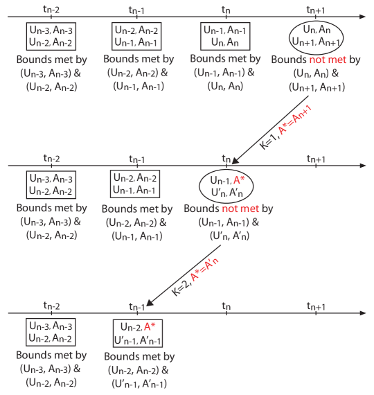
Figure 1: Visualization of the Backtracking Algorithm 2 using the alternating minimization (5.5) with $K=2$. In each square/circle we show the starting guess and the solution of the incremental problem.

Box $\bm{1}$. Implementation of (5.6)

function ERG
INPUT: $\bm{U}_{1},\,\bm{U}_{2},\,\bm{A}$
COMPUTE: $$E=\sum_{\Omega_{e}^{h}\in\mathcal{T}^{h}}\;\sum_{i=1}^{n_{gp}}w_{e,i}j_{e,i}\bigg{[}R\big{(}\bm{N}_{\beta}(\bm{x}_{e,i})\bm{A}\big{)}\psi_{0}^{+}\big{(}\bm{B}_{\bm{u}}(\bm{x}_{e,i})(\bm{U}_{1}+\bm{U}_{2})\big{)}+\psi_{0}^{-}\big{(}\bm{B}_{\bm{u}}(\bm{x}_{e,i})(\bm{U}_{1}+\bm{U}_{2})\big{)}\bigg{]}$$ function GRAD
INPUT: $\bm{A}$
COMPUTE: $$G=\frac{g_{c}\ell}{2}\sum_{\Omega_{e}^{h}\in\mathcal{T}^{h}}\;\sum_{i=1}^{n_{gp}}w_{e,i}j_{e,i}\bigg{[}\bm{B}_{\beta}^{T}(\bm{x}_{e,i})\bm{B}_{\beta}(\bm{x}_{e,i})\bm{A}\cdot\bm{A}\bigg{]}$$ function DIS
INPUT: $\bm{A}$
COMPUTE: $$D=\frac{g_{c}}{2\ell}\sum_{\Omega_{e}^{h}\in\mathcal{T}^{h}}\;\sum_{i=1}^{n_{gp}}w_{e,i}j_{e,i}\bigg{[}\bm{N}_{\beta}^{T}(\bm{x}_{e,i})\bm{N}_{\beta}(\bm{x}_{e,i})\bm{A}\cdot\bm{A}\bigg{]}$$ To compute $\mathcal{E}(t_{n+1},\bm{u}_{n+1},\beta_{n+1})-\mathcal{E}(t_{n},\bm{u}_{n},\beta_{n})+\mathcal{D}(\beta_{n},\beta_{n+1})$, use: 1. function ERG with INPUT: $\bm{U}_{1}=\bm{U}_{n+1}$, $\bm{U}_{2}=\bm{U}_{D,n+1}$, $\bm{A}=\bm{A}_{n+1}$
xxxxxxxOUTPUT: $E1$ 2. function GRAD with INPUT: $\bm{A}=\bm{A}_{n+1}$
xxxxxxxOUTPUT: $G1$ 3. function DIS with INPUT: $\bm{A}=\bm{A}_{n+1}$
xxxxxxxOUTPUT: $D1$ 4. function ERG with INPUT: $\bm{U}_{1}=\bm{U}_{n}$, $\bm{U}_{2}=\bm{U}_{D,n}$, $\bm{A}=\bm{A}_{n}$
xxxxxxxOUTPUT: $E2$ 5. function GRAD with INPUT: $\bm{A}=\bm{A}_{n}$
xxxxxxxOUTPUT: $G2$ 6. function DIS with INPUT: $\bm{A}=\bm{A}_{n}$
xxxxxxxOUTPUT: $D2$ 7. COMPUTE: $(E1+G1+D1)-(E2+G2+D2)$ To compute Upper Bound $UB$ (refer to Eq. (3.15) and Eq. (3.24)), use: 1. function ERG with INPUT: $\bm{U}_{1}=\bm{U}_{n}$, $\bm{U}_{2}=\bm{U}_{D,n+1}$, $\bm{A}=\bm{A}_{n}$
xxxxxxxOUTPUT: $E1$ 2. function ERG with INPUT: $\bm{U}_{1}=\bm{U}_{n}$, $\bm{U}_{2}=\bm{U}_{D,n}$, $\bm{A}=\bm{A}_{n}$
xxxxxxxOUTPUT: $E2$ 3. COMPUTE: $UB=E1-E2$ To compute Lower Bound $LB$ (refer to Eq. (3.16) and Eq. (3.24)), use: 1. function ERG with INPUT: $\bm{U}_{1}=\bm{U}_{n+1}$, $\bm{U}_{2}=\bm{U}_{D,n+1}$, $\bm{A}=\bm{A}_{n+1}$
xxxxxxxOUTPUT: $E1$ 2. function ERG with INPUT: $\bm{U}_{1}=\bm{U}_{D,n+1}$, $\bm{U}_{2}=\bm{U}_{D,n}$, $\bm{A}=\bm{A}_{n+1}$
xxxxxxxOUTPUT: $E2$ 3. COMPUTE: $LB=E1-E2$

Data: $N,\,K,\,\eta,\,(\bm{U}_{0},\,\bm{A}_{0})$

Result: $(\bm{U}_{n},\,\bm{A}_{n})$ $n=1,\ldots,N$

set

      1 $n=0$

      2 $\bm{A}^{0}=\bm{A}_{0}$, $\bm{U}^{0}=\bm{U}_{0}$

3repeat

      4 solve

            5 input : $\bm{A}^{0}$, $\bm{U}^{0}$, $\bm{A}_{n}$

            6 Algorithm 1: $(\bm{U}_{n+1},\,\bm{A}_{n+1})=\textsc{argmin }\mathcal{F}(t_{n+1},\bm{U},\bm{A};\,\bm{A}_{n})$

            7 output : $\bm{U}_{n+1}$, $\bm{A}_{n+1}$

            

      

      set

            8 $\bm{A}^{0}=\bm{A}_{n+1}$, $\bm{U}^{0}=\bm{U}_{n+1}$

      

      9if inequality (5.6) is met then

            10 $n\leftarrow n+1$ (proceed to the next step)

      else

            11 $b=0$ (back steps counter)

            12 repeat

                  13 $n\leftarrow n-1$ (go back by one step)

                  14 $b=b+1$

                  15 solve

                        16 input : $\bm{A}^{0}$, $\bm{U}^{0}$, $\bm{A}_{n}$

                        17 Algorithm 1: $(\bm{U}_{n+1},\,\bm{A}_{n+1})=\textsc{argmin }\mathcal{F}(t_{n+1},\bm{U},\bm{A};\,\bm{A}_{n})$

                        18 output : $\bm{U}_{n+1}$, $\bm{A}_{n+1}$

                        

                  

                  set

                        19 $\bm{A}^{0}=\bm{A}_{n+1}$, $\bm{U}^{0}=\bm{U}_{n+1}$

                  

            until inequality (5.6) is met or $b=K$

            20$n\leftarrow n+1$ (proceed to the next step)

      

until $n=N$

Algorithm 2 Backtracking Algorithm.

6 Numerical examples

In this section, we present representative numerical experiments to illustrate the perfomance of the energetic formulation and of the numerical procedure to obtain energetic solutions. We compare these solutions, which we will refer to as approximated energetic solutions, with those obtained by the standard procedure of simply solving the weak form of the Euler–Lagrange equations [63, 48, 80, 62, 5]. The problems that we consider are:

• Single edge notched tension test;

• Single edge notched shear test;

• $3d$ $L-$shaped panel test;

• $3d$ Symmetric bending test.

The first two are classical $2d$ benchmark problems where the specimens are assumed in plane strain conditions, whereas the last two are $3d$ bending tests of a concrete panel and a cement paste beam which we compare with experimental results. All the numerical simulations are carried out with $\psi_{0}^{+}$ and $\psi_{0}^{-}$ given by

$$\psi_{0}^{\pm}(\bm{\varepsilon})=\frac{\lambda}{2}(\operatorname{\mathsf{tr}}\bm{\varepsilon}^{\pm})^{2}+\mu\bm{\varepsilon}^{\pm}\colon\bm{\varepsilon}^{\pm}$$

with $\lambda$ and $\mu$ the Lamè constants, whereas $\bm{\varepsilon}^{+}$ and $\bm{\varepsilon}^{-}$ are obtained by the spectral decomposition of $\bm{\varepsilon}$ introduced in [62, 63] as

$$\bm{\varepsilon}^{+}=\sum_{a=1}^{3}\langle\varepsilon_{a}\rangle_{+}\bm{n}_{a}\otimes\bm{n}_{a}\quad\quad\quad\bm{\varepsilon}^{-}=\sum_{a=1}^{3}\langle\varepsilon_{a}\rangle_{-}\bm{n}_{a}\otimes\bm{n}_{a}\,,$$

where $\varepsilon_{a}$, $\bm{n}_{a}$, $a=1,2,3$, are the principal strains and the principal strain directions of $\bm{\varepsilon}$, respectively, and for $x\in\mathbb{R}$, $\langle x\rangle_{+}=(x+|x|)/2$ and $\langle x\rangle_{-}=(x-|x|)/2$. We also use $g(\beta)=(1-\beta)^{2}$ as degradation function according to what noted in Remark 3.3$(iii)$ and, for the residual stiffness, we set $k=10^{-4}$ (see [7, Sec. 5] and discussion therein). We apply monotonic displacement control by comparing the response for different displacement increments $\Delta w$. As for the value of the penalization factor $\epsilon$ to enforce crack irreversibility, this depends on the problem at hand. For its selection, we tested different values of $\epsilon$ and chose the one that was ensuring that the dissipation $\mathcal{D}(\beta_{n},\,\beta_{n+1})$, $n=0,\,\ldots,\,N-1$, was non-negative and the problem conditioning was not jeopardized. The values of the tolerances $tol_{\bm{U}}$ and $tol_{\bm{A}}$ that control the convergence of Algorithm 1 and the two-sided energy inequality tolerance $\eta$ have been all set equal, in the respective units, to $10^{-5}$. We run our examples with two different values of $K$: $K=0$ to obtain discrete solutions by the standard procedure such as in [62, 30] where one does not control the energy estimates (5.6) and $K>0$ to obtain discrete solutions with the backtracking algorithm. In this latter case, the value of $K$ is chosen so that we can always go back as many time steps as necessary to obtain discrete solutions meeting (5.6) along the whole evolution. For the present simulations, for instance, by taking $K=50$ we could observe that we were never going back more than $10\div 30$ steps. This will be easily verified for each of the numerical simulations by inspecting the plot of the terms that enter (5.6) and noting that the estimates are met by the discrete solutions when the backtracking is active.

6.1 Single edge notched tension test

The single edge notched tension (SENT) test is a classical benchmark problem which is used for a wide range of applications [8] and is well studied also in the numerical literature [63, 48, 80, 62, 5]. It consists of a square specimen with a single horizontal notch located at mid-height of the left edge with length equal to half the edge length, and is subject to constant tension on the top edge. In this paper, we consider the same mechanical model analysed in [63]. The geometric properties and boundary conditions of the specimen are shown in Figure 2$(a)$, with $\bm{u}=\bm{0}$ at the point of coordinates $(0,\,0)$ and $u_{z}=0$ on the bottom edge; $u_{y}=0$ and non–homogeneous Dirichlet condition $u_{z}=w$ on the top edge whereas all the other parts of the boundary including the slit are traction free. The elastic constants are chosen as $\lambda=121.1538\,\mathrm{kN/mm^{2}}$ and $\mu=80.7692\,\mathrm{kN/mm^{2}}$, the critical energy release rate as $g_{c}=2.7\,\,\mathrm{N/mm}$ and the internal length as $\ell=0.0175\,\mathrm{mm}$. Figure 2$(b)$ displays the unstructured finite element mesh used for the simulations. We use linear finite elements for the approximation of the displacement field and of the phase-field. The mesh is thus formed by $6062$ triangular elements with $3088$ nodes. In order to capture properly the crack pattern, since under constant tension the crack propagates straight, we refine the mesh in this zone with an effective element size $h\approx 0.005\,\mathrm{mm}<\ell/2$ and for a bandwidth of about $2\,\mathrm{mm}$.

$\begin{array}[]{cc}\includegraphics[width=140.84256pt]{SENTgeo-vr1.pdf}&\includegraphics[width=117.36761pt]{SENTmesh-vr1.pdf}\\ (a)&(b)\end{array}$

Figure 2: Example 6.1. Single edge notched tension test. $(a)$ Specimen geometry and boundary conditions. $(b)$ Unstructured finite element mesh.

We analyse the behaviour of the model for a monotone applied displacement $w$ resulting from the application of the following displacement increments: $\Delta~{}w~{}=~{}10^{-4}~{}\,~{}\mathrm{mm}$, $\Delta~{}w~{}=~{}10^{-5}~{}\,~{}\mathrm{mm}$ and $\Delta~{}w~{}=~{}10^{-6}~{}\,~{}\mathrm{mm}$. We take $\epsilon=10^{-6}$ and we evaluate then the reaction force $F_{z}$ on the top edge $\Gamma_{top}\subseteq\partial\Omega$ given by

$$F_{z}=\int_{\Gamma_{top}}\,\bm{\sigma}\bm{n}\cdot\bm{n}\,\operatorname{\mathrm{d}\mathit{s}}$$

where $\bm{n}$ is the outward normal to this part of the boundary, and the energetic terms $\mathcal{E}(t_{n+1},\bm{U}_{n+1},\bm{A}_{n+1})$ and $\mathcal{D}(\bm{A}_{n},\bm{A}_{n+1})$, $n=0,1,\ldots,N-1$ with $N$ the total number of increments $\Delta w$.

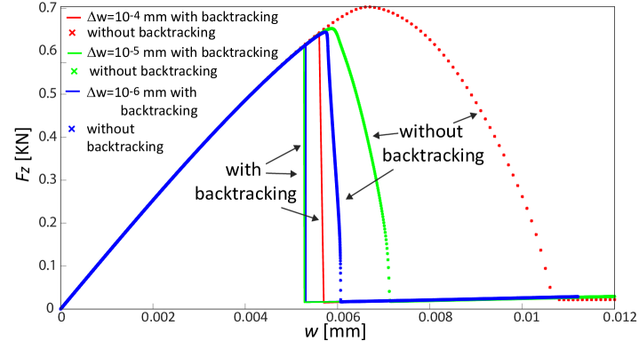
Figure 3: Example 6.1. Single edge notched tension test. Load–displacement curves for different displacement increments $\Delta w$ and different schemes, using the backtracking algorithms describing the evolution of the approximate energetic solutions and without applying the backtracking algorithm.

The variation of $F_{z}$ with $w$ for the different displacement increments and the different algorithms are displayed in Figure 3. By applying the backtracking algorithm (Algorithm 2 with $K>0$) the load-displacement curves display a similar response independent of the displacement increment $\Delta w$. This is in contrast with the behaviour associated with the solutions of Algorithm 2 with $K=0$, where the backtracking option is not active. In this case, for the range of values used for $\Delta w$, the behaviour is sensitive with respect to $\Delta w$, though for small values of $\Delta w$ the response converges towards a definite configuration. Both numerical strategies identify a strong decreasing structural response, but the one described by the backtracking strategy occurs prior to that corresponding to the standard solution. Furthermore, for both type of solutions, the load-displacement curve displays a residual force $F_{z}$ of the fully damaged specimen which is related to the value of $\delta$, that defines the ‘residual’ energy after complete damage.

$\begin{array}[]{c}\includegraphics[width=281.68513pt]{SENTEnergVarWithWithoutBT4.pdf}\\ (a)\\ \begin{array}[]{cc}\includegraphics[width=230.04309pt]{SENTEnrgEstWithoutBT4.pdf}&\includegraphics[width=230.04309pt]{SENTEnrgEstWithBT4.pdf}\\ (b)&(c)\end{array}\end{array}$

Figure 4: Example 6.1. Single edge notched tension test. Results for $\Delta w=10^{-4}\,\mathrm{mm}$. $(a)$ Evolution of the total energy $\mathcal{E}(t_{n+1},\bm{U}_{n+1},\bm{A}_{n+1})+\sum_{i=0}^{n}\mathcal{D}(\bm{A}_{i},\bm{A}_{i+1})$ for $n=0,1,\ldots,N-1$, , without backtracking $(K=0)$ and with backtracking. Evolution of the total incremental energy $\mathcal{E}_{n+1}-\mathcal{E}_{n}+\mathcal{D}_{n,n+1}$, the lower bound $LB_{n,n+1}$ and the upper bound $UB_{n,n+1}$ which enter the two-sided energy estimate (5.6), $n=0,1,\ldots,N-1$, for the scheme $(b)$ without backtracking and $(c)$ with backtracking.

$\begin{array}[]{c}\includegraphics[width=281.68513pt]{SENTEnergVarWithWithoutBT5.pdf}\\ (a)\\ \begin{array}[]{cc}\includegraphics[width=230.04309pt]{SENTEnrgEstWithoutBT5.pdf}&\includegraphics[width=230.04309pt]{SENTEnrgEstWithBT5.pdf}\\ (b)&(c)\end{array}\end{array}$

Figure 5: Example 6.1. Single edge notched tension test. Results for $\Delta w=10^{-5}\,\mathrm{mm}$. $(a)$ Evolution of the total energy $\mathcal{E}(t_{n+1},\bm{U}_{n+1},\bm{A}_{n+1})+\sum_{i=0}^{n}\mathcal{D}(\bm{A}_{i},\bm{A}_{i+1})$ for $n=0,1,\ldots,N-1$, without backtracking $(K=0)$ and with backtracking. Evolution of the total incremental energy $\mathcal{E}_{n+1}-\mathcal{E}_{n}+\mathcal{D}_{n,n+1}$, the lower bound $LB_{n,n+1}$ and the upper bound $UB_{n,n+1}$ which enter the two-sided energy estimate (5.6), $n=0,1,\ldots,N-1$, for the scheme $(b)$ without backtracking and $(c)$ with backtracking.

$\begin{array}[]{c}\includegraphics[width=281.68513pt]{SENTEnergVarWithWithoutBT6-vr2.pdf}\\ (a)\\ \begin{array}[]{cc}\includegraphics[width=230.04309pt]{SENTEnrgEstWithoutBT6.pdf}&\includegraphics[width=230.04309pt]{SENTEnrgEstWithBT6.pdf}\\ (b)&(c)\end{array}\end{array}$

Figure 6: Example 6.1. Single edge notched tension test. Results for $\Delta w=10^{-6}\,\mathrm{mm}$. $(a)$ Evolution of the total energy $\mathcal{E}(t_{n+1},\bm{U}_{n+1},\bm{A}_{n+1})+\sum_{i=0}^{n}\mathcal{D}(\bm{A}_{i},\bm{A}_{i+1})$ for $n=0,1,\ldots,N-1$, without backtracking $(K=0)$ and with backtracking. Evolution of the total incremental energy $\mathcal{E}_{n+1}-\mathcal{E}_{n}+\mathcal{D}_{n,n+1}$, the lower bound $LB_{n,n+1}$ and the upper bound $UB_{n,n+1}$ which enter the two-sided energy estimate (5.6), $n=0,1,\ldots,N-1$, for the scheme $(b)$ without backtracking and $(c)$ with backtracking.

The energy variation associated with the solutions computed without the backtracking $(K=0)$ and with the backtracking option active $(K>0)$ are depicted in Figure 4 to Figure 6 for the three displacement driven conditions, $\Delta w=10^{-4}\,\mathrm{mm}$, $\Delta w=10^{-5}\,\mathrm{mm}$ and $\Delta w=10^{-6}\,\mathrm{mm}$, respectively. Figure 4$(a)$, Figure 5$(a)$ and Figure 6$(a)$ show the evolution of the total energy $\mathcal{E}(t_{n+1},\bm{U}_{n+1},\bm{A}_{n+1})+\sum_{i=0}^{n}\mathcal{D}(\bm{A}_{i},\bm{A}_{i+1})$, the current free energy $\mathcal{E}_{n+1}$ and the total dissipation $\sum_{i=0}^{n}\mathcal{D}_{i,i+1}$, for $n=0,1,\ldots,N-1$. The energy paths obtained without backtracking display a bubble shape when damage starts to propagate due to the gradual substantial reduction of the free energy because of the reduction of the elastic energy and of the increase of the dissipation energy. Such bubble is not present using the backtracking given that in this case the damage evolution is faster. For both the schemes, when the crack completes its propagation along half specimen, the total energy increases very little, due to the regularization parameter $\delta$, and is almost equal to the accumulated dissipated energy.

Figure 4$(b)$, Figure 5$(b)$ and Figure 6$(b)$ display the total incremental energy $\mathcal{E}_{n+1}-\mathcal{E}_{n}+\mathcal{D}_{n,n+1}$, the upper bound $UB_{n,n+1}$ and the lower bound $LB_{n,n+1}$, for $n=0,\,\ldots,N-1$ associated with the solutions computed without activating the backtracking scheme $(K=0)$, whereas Figure 4$(c)$, Figure 5$(c)$ and Figure 6$(c)$ contain the same type of plots relative to the approximate energetic solutions. When damage starts to develop, the alternate minimization Algorithm 1 fails to provide an appropriate energetic solution to the problem. As a result, the sequence of discrete solutions evolves along a path of local minima, whose energy deviates substantially from the one associated with global minimization. The energetic bounds (5.6), and more specifically the lower bound, are then violated by the computed solutions. The two-sided energy inequality (5.6) is met only during the initial stage when the specimen remains elastic and in the last stage of the cracking process showing that the algorithm jumps back into a state of significantly lower energy. By contrast, with the backtracking option active, we avoid the wrong forward path obtained by the standard scheme, for we restart with ‘better’ local minima and we are able to obtain a final path of the energy difference which lies between the two bounds.

$\begin{array}[]{cccc}\text{$(a)$ Without backtracking}&&&\\ \includegraphics[width=117.36761pt]{SENTNoBT05d500.pdf}&\includegraphics[width=117.36761pt]{SENTNoBT05d550.pdf}&\includegraphics[width=117.36761pt]{SENTNoBT05d600.pdf}&\includegraphics[width=117.36761pt]{SENTNoBT05d700.pdf}\\ w=0.005\,\mathrm{mm}&w=0.0055\,\mathrm{mm}&w=0.006\,\mathrm{mm}&w=0.007\,\mathrm{mm}\\[6.45831pt] \text{$(b)$ With backtracking}&&&\\ \includegraphics[width=117.36761pt]{SENTBT5d500.pdf}&\includegraphics[width=117.36761pt]{SENTBT5d537.pdf}&\includegraphics[width=117.36761pt]{SENTBT5d550.pdf}&\includegraphics[width=117.36761pt]{SENTBT5d700.pdf}\\ w=0.005\,\mathrm{mm}&w=0.00537\,\mathrm{mm}&w=0.0055\,\mathrm{mm}&w=0.007\,\mathrm{mm}\end{array}$

Figure 7: Example 6.1. Single edge notched tension test. Phase field distribution at different stages of the total displacement $w$ applied on the specimen top edge. Results for $\Delta w=10^{-5}\,\mathrm{mm}$. In the damage maps, the yellow corresponds to $\beta=1-\delta$ with $\delta=10^{-4}$ given that we are considering a partially damage profile, whereas the blue corresponds to solid material for which $\beta=0$.

$\begin{array}[]{ccc}\includegraphics[width=154.9261pt]{SENTForceDisp4.pdf}&\includegraphics[width=154.9261pt]{SENTForceDisp5.pdf}&\includegraphics[width=154.9261pt]{SENTForceDisp6.pdf}\\ (a)&(b)&(c)\end{array}$

Figure 8: Example 6.1. Single edge notched tension test. Load–displacement curves associated with the intermediate energetic solutions obtained with the backtracking algorithm and for the different displacement increments. $(a)$ $\Delta w=10^{-4}\,\mathrm{mm}$; $(b)$ $\Delta w=10^{-5}\,\mathrm{mm}$ and $(c)$ $\Delta w=10^{-6}\,\mathrm{mm}$.

To get some further insight on the structure of the energetic solutions, we recall that each loading step is solved by the alternating minimization method with the last converged approximate energetic solution as starting guess. The solution that we thus compute is in fact a local minimizer, unless it verifies the energetic bounds (5.6). By the backtracking algorithm we are looking for a solution close to the starting guess which meets the energetic bounds, thus it is more likely to be a global minimizer. As a result, if the energetic bounds are not met, the algorithm move one step backward (as we have skteched in Figure 1) and solves again the previous step but with different starting, guess given by the last computed damage value, thus defining a lower energy state. If also such solution does not meet the energetic bounds, the algorithm moves a further step back and the process is repeated until the bounds are met or we reach the maximum number $K$ that we have set to go backward. Only then the algorithm proceeds one step forward. In our simulations we never reached such limit value for $K$ which was set equal to $50$. Figure 7 displays the distribution of the phase-field $\beta$ at the different stages of the evolutive process as computed by the two numerical schemes. Consistently with the procedure described above, the damage profile displays with the backtracking option active a faster evolution and higher dissipation when compared with the basic variant. This behaviour is also confirmed by the numerical experiments of [66] where the AT1 regularized formulation of fracture is considered without the splitting of the free elastic energy $\psi_{0}$.

Given that with the backtracking option active, we go backward and forward, obtaining energetic solutions for the same displacement but with increasing damage and therefore lower resultant load, we save these solutions, for which the total energy remains between the two energetic bounds. Figure 8 displays the load-displacement curve associated with such intermediate configurations. For instance, for the step increment $\Delta w=10^{-4}\,\mathrm{mm}$, the path zigzags down to the curve because with such size of the increment, the two sided energetic bounds are more distant from each other, leaving more room to move within the bounds. Such range between the bounds is reduced by reducing the displacement increment $\Delta w$ and so is the zigzaged path.

6.2 Single edge notched shear test

We now consider the same square plate with horizontal notch as in the previous example but this time subject to pure shear deformation. This problem has received a lot of attention in the literature on phase-field modelling of brittle fracture [16, 62, 63] for its simple setup and for displaying an asymmetric failure pattern. Due to a non–trivial combination of local tension-compression and loading–unloading processes, the crack propagates towards the lower right corner of the square plate. The geometric setup and boundary conditions are displayed in Figure 9$(a)$.

$\begin{array}[]{cc}\includegraphics[width=164.31752pt]{SENSTgeo-vr1.pdf}&\includegraphics[width=93.89265pt]{SENSTmesh-vr1.pdf}\\ (a)&(b)\end{array}$

Figure 9: Example 6.2. Single edge notched shear test. $(a)$ Geometry and boundary conditions. $(b)$ Unstructured finite element mesh.

The vertical displacement component is constrained on all four sides of the domain. The botton edge is also constrained along the horizontal direction whereas the top edge presents a prescribed nonhomogeneous Dirichlet boundary condition $u_{z}=w$. The same material properties are used as for the previous example. The characteristic length is now set equal to $\ell=0.001\,\mathrm{mm}$. Figure 9$(b)$ displays the unstructured finite element mesh with $7573$ triangular elements and $3878$ nodes which has been refined in the lower right part of the domain $\Omega$ where the crack is expected to propagate [16, 63]. The characteristic element size in this region is $h\approx 0.005\,\mathrm{mm}<\ell/2$. The finite element approximations for the displacement and phase-field is the same as in the previous example. We consider displacement-driven loading by the application of two constant displacement increments $\Delta w=10^{-4}\,\mathrm{mm}$ and $\Delta w=10^{-5}\,\mathrm{mm}$, and take, for this example, the penalization factor $\epsilon$ equal to $10^{-5}$. We have then evaluated, for each case, the energetic terms that enter (5.6) and the reaction force $F_{z}$ on the top edge $\Gamma_{top}\subseteq\partial\Omega$ given by

$$F_{z}=\int_{\Gamma_{top}}\,\bm{\sigma}\bm{n}\cdot\bm{t}\,\operatorname{\mathrm{d}\mathit{s}}$$

where $\bm{t}$ is the tangent to the top edge and $\bm{n}$ is the outward normal to this part of the boundary.

$\begin{array}[]{c}\includegraphics[width=234.73523pt]{SENSTForceDisplWithWithoutBT.pdf}\end{array}$

Figure 10: Example 6.2. Single edge notched shear test. Load–displacement curves for different displacement increments $\Delta w$ and different schemes, using the backtracking algorithms describing the evolution of the approximate energetic solutions and without applying the backtracking algorithm.

Figure 10 displays the load-displacement curves corresponding to the approximate energetic solutions and to the solutions obtained without using the backtracking algorithm, for the two different applications of $\Delta w$. Likewise the previous example, the structural response obtained by the approximate energetic solutions is almost the same for $\Delta w=10^{-4}\,\mathrm{mm}$ and $\Delta w=10^{-5}\,\mathrm{mm}$.

$\begin{array}[]{cc}\includegraphics[width=230.04309pt]{SENSTForceDispl4.pdf}&\includegraphics[width=230.04309pt]{SENSTForceDispl5.pdf}\\ (a)&(b)\end{array}$

Figure 11: Example 6.2. Single edge notched shear test. Load–displacement curves associated with the intermediate energetic solutions obtained with the backtracking algorithm for the displacement increment $(a)$ $\Delta w=10^{-4}\,\mathrm{mm}$ and $(b)$ $\Delta w=10^{-5}\,\mathrm{mm}$.

The load-displacement curves corresponding also to the intermediate solutions are, by contrast, displayed in Figure 11. For the step increment $\Delta w=10^{-4}\,mm$ the curve zigzags towards the softenning part of the curve, whereas for the smaller increment $\Delta~{}w=10^{-5}~{}\,~{}\mathrm{mm}$, the two bounds get closer and the curve results smoother with only two small jumps. The variations of the total energies of the solutions computed with the two numerical schemes and for $\Delta w=10^{-4}\,\mathrm{mm}$ and $\Delta w=10^{-5}\,\mathrm{mm}$ are plotted in Figure 12 and Figure 13, respectively. Figure 12$(a)$ and Figure 13$(a)$ show, for the respective $\Delta w$, the evolution of the total energetic of the system, the total free energy and the accumulated dissipation. Figure 12$(b)$ and Figure 13$(b)$, and Figure 12$(c)$ and Figure 13$(c)$ display the total incremental energy $\mathcal{E}_{n+1}-\mathcal{E}_{n}+\mathcal{D}_{n,n+1}$, the upper bound $UB_{n,n+1}$ and the lower bound $LB_{n,n+1}$, for $n=0,\,\ldots,N-1$. We thus verify that also for this problem, the activation of the backtracking algorithm is needed to select the ‘right’ forward path of the lowest energy content given by approximate energetic solutions. Figure 14 finally displays the phase-field distribution at different stages of the displacement $w$ for the two numerical scheme showing that with the backtracking algorithm we obtain a faster evolution when compared with the basic scheme.

$\begin{array}[]{c}\includegraphics[width=281.68513pt]{SENSTEnrgVarWithWithoutBT4.pdf}\\ (a)\\ \begin{array}[]{cc}\includegraphics[width=230.04309pt]{SENSTEnrgEstimatesWithoutBT4.pdf}&\includegraphics[width=230.04309pt]{SENSTEnrgEstimatesWithBT4.pdf}\\ (b)&(c)\end{array}\end{array}$

Figure 12: Example 6.2. Single edge notched shear test. Results for $\Delta w=10^{-4}\,\mathrm{mm}$. $(a)$ Evolution of the total energy $\mathcal{E}(t_{n+1},\bm{U}_{n+1},\bm{A}_{n+1})+\sum_{i=0}^{n}\mathcal{D}(\bm{A}_{i},\bm{A}_{i+1})$ for $n=0,1,\ldots,N-1$, without backtracking $(K=0)$ and with backtracking. Evolution of the total incremental energy $\mathcal{E}_{n+1}-\mathcal{E}_{n}+\mathcal{D}_{n,n+1}$, the lower bound $LB_{n,n+1}$ and the upper bound $UB_{n,n+1}$ which enter the two-sided energy estimate (5.6), $n=0,1,\ldots,N-1$, for the scheme $(b)$ without backtracking and $(c)$ with backtracking.

$\begin{array}[]{c}\includegraphics[width=281.68513pt]{SENSTEnrgVarWithWithoutBT5.pdf}\\ (a)\\ \begin{array}[]{cc}\includegraphics[width=230.04309pt]{SENSTEnrgEstimatesWithoutBT5.pdf}&\includegraphics[width=230.04309pt]{SENSTEnrgEstimatesWithBT5.pdf}\\ (b)&(c)\end{array}\end{array}$

Figure 13: Example 6.2. Single edge notched shear test. Results for $\Delta w=10^{-5}\,\mathrm{mm}$. $(a)$ Evolution of the total energy $\mathcal{E}(t_{n+1},\bm{U}_{n+1},\bm{A}_{n+1})+\sum_{i=0}^{n}\mathcal{D}(\bm{A}_{i},\bm{A}_{i+1})$ for $n=0,1,\ldots,N-1$, without backtracking $(K=0)$ and with backtracking. Evolution of the total incremental energy $\mathcal{E}_{n+1}-\mathcal{E}_{n}+\mathcal{D}_{n,n+1}$, the lower bound $LB_{n,n+1}$ and the upper bound $UB_{n,n+1}$ which enter the two-sided energy estimate (5.6), $n=0,1,\ldots,N-1$, for the scheme $(b)$ without backtracking and $(c)$ with backtracking.

$\begin{array}[]{cccc}\text{$(a)$ Without backtracking}&&&\\ \includegraphics[width=117.36761pt]{b04d125-vr1.pdf}&\includegraphics[width=117.36761pt]{b04d150-vr1.pdf}&\includegraphics[width=117.36761pt]{b04d175-vr1.pdf}&\includegraphics[width=117.36761pt]{b04d200-vr1.pdf}\\ w=0.0125\,\mathrm{mm}&w=0.0150\,\mathrm{mm}&w=0.0175\,\mathrm{mm}&w=0.0200\,\mathrm{mm}\\[6.45831pt] \text{$(b)$ With backtracking}&&&\\ \includegraphics[width=117.36761pt]{bT4d125-vr1.pdf}&\includegraphics[width=117.36761pt]{bT4d150-vr1.pdf}&\includegraphics[width=117.36761pt]{bT4d175-vr1.pdf}&\includegraphics[width=117.36761pt]{bT4d200-vr1.pdf}\\ w=0.0125\,\mathrm{mm}&w=0.0150\,\mathrm{mm}&w=0.0175\,\mathrm{mm}&w=0.0200\,\mathrm{mm}\\ \end{array}$

Figure 14: Example 6.2. Single edge notched shear test. Phase field distribution at different stages of the total displacement $w$ applied on the specimen top edge. Results for $\Delta w=10^{-5}\,\mathrm{mm}$. In the damage maps, the yellow corresponds to $\beta=1-\delta$ with $\delta=10^{-4}$ given that we are considering a partially damage profile, whereas the blue corresponds to solid material for which $\beta=0$.

6.3 Three dimensional $L-$shaped panel test

We analyze now the $3d$ crack propagation in an $L$–shaped concrete panel as benchmark for crack initiation [5, 21, 40, 60] and, likewise Example 6.2, to demonstrate the ability of the phase-field variational formulation to describe curved crack patterns. The geometry and boundary conditions are displayed in Figure 15$(a)$, and correspond to the experimental setup given in [82]. All the points of the face of equation $y=0$ are fully restrained whereas those belonging to the line of equation $x=470\,\mathrm{mm}$, $y=250\,\mathrm{mm}$ and $0\,\mathrm{mm}\leq z\leq 100\,\mathrm{mm}$ present prescribed values for $v$ and free the other degrees of freedom.

$\begin{array}[]{cc}\includegraphics[width=211.26027pt]{LshapeGeo.pdf}&\includegraphics[width=187.78531pt]{Lshape3DMesh-vr1.pdf}\\ (a)&(b)\end{array}$

Figure 15: Example 6.3. $3d$ $L-$shaped panel test. $(a)$ Geometric setup. $(b)$ Unstructured finite element mesh.

The concrete material properties chosen are the same as given in [82] with the Young modulus $E=25.85\,\mathrm{kN/mm^{2}}$, the Poisson ratio $\nu=0.18$, the critical energy release rate $g_{c}=0.095\,\,\mathrm{N/mm}$ and the internal length $\ell=20\,\mathrm{mm}$. The unstructured finite element mesh is shown in Figure 15$(b)$ and consists of $44880$ tetrahedral elements and $68470$ nodes. No initial crack is prescribed. However, since we expect that this starts at the interior corner of the $L-$shape, we have refined therein the mesh with a characteristic finite element length equal to $h=6.25\,\mathrm{mm}<\ell/2$ in order to resolve properly the crack pattern.

$\begin{array}[]{c}\includegraphics[width=305.15292pt]{LshapeForceVsDispWithWithoutBT3-vr1.pdf}\end{array}$

Figure 16: Example 6.3. $3d$ $L-$shaped panel test. Load–displacement curves in the case the backtracking algorithm is activated and for the case without applying the backtracking algorithm.

The numerical simulations have been carried out by applying a monotone loading history for the nonhomogeneous Dirichlet boundary condition $v$ by means of the application of constant displacement increments $\Delta v=10^{-3}\,\mathrm{mm}$. For this example, the penalization factor $\epsilon$ has been set equal to $10^{-4}$. Figure 16 displays the resulting load-displacement curves with $(K>0)$ and without $(K=0)$ the backtracking option active. We observe that the two curves are practically identical until the peak, but they then differentiate each other for a short range of the applied displacement $v$ in the post peak, where we verify only a minor occurrence of backtracking, for then to display again the same behaviour starting from around $v=0.3\,\mathrm{mm}$. Our numerical results compare quite well with those obtained by [60, 21], but they all differentiate in a relevant manner from the experimental findings of [82] in the detection of the peak value and of the residual load. This behaviour was also noted in [60]. We ascribe the difference of results to the quasi–brittle model we have used for the concrete which does not account for plastic deformations prior to the damage and for cohesive forces on the crack surfaces. By applying a mixed-mode cohesive crack model but with an energy–based crack criterion, on the other hand, [68] can obtain good agreement with the experiments of [82].

$\begin{array}[]{c}\includegraphics[width=230.04309pt]{LshapeEnergVarWithWithoutBT3-vr1.pdf}\\ (a)\\ \begin{array}[]{cc}\includegraphics[width=230.04309pt]{LshapeEnrgEstWithoutBT3-vr1.pdf}&\includegraphics[width=230.04309pt]{LshapeEnrgEstWithBT3-vr1.pdf}\\ (b)&(c)\end{array}\end{array}$

Figure 17: Example 6.3. $3d$ $L-$shaped panel test. Results for $\Delta v=10^{-3}\,\mathrm{mm}$. $(a)$ Evolution of the total energy $\mathcal{E}(t_{n+1},\bm{U}_{n+1},\bm{A}_{n+1})+\sum_{i=0}^{n}\mathcal{D}(\bm{A}_{i},\bm{A}_{i+1})$ for $n=0,1,\ldots,N-1$, without backtracking $(K=0)$ and with backtracking. Evolution of the total incremental energy given by $\mathcal{E}_{n+1}-\mathcal{E}_{n}+\mathcal{D}_{n,n+1}$ and of the lower $LB_{n,n+1}$ and upper bound $UB_{n,n+1}$ which enter the two-sided energy estimate (5.6), $n=0,1,\ldots,N-1$, for the scheme $(b)$ without backtracking and $(c)$ with backtracking.

The confirmation of the aforementioned behaviour is obtained by analysing the evolution of the total energetics of the computed solutions displayed in Figure 17. The discrete computed solutions obtained by the the alternate minimization method without backtracking fails to yield approximate energetic solutions. Figure 17$(b)$ shows that the two-sided energy inequality (5.6) is satisfied only in the initial stage when the specimen stays mainly elastic and in the last stage when the specimen experiences the same damage pattern, that is, when the algorithm fall back to lower energy states, whereas it is violated for other values of $v$. With the backtracking option active, by contrast, Figure 17$(c)$ shows that the alternate minimization is capable of detecting a lower energy path during the whole evolution which is defined by the approximate energetic solutions that meet the two–sided energy inequality. Finally, Figure 18 displays the phase-field distribution on the plane $z=50\,\mathrm{mm}$ at different stages of the displacement $v$ for the two numerical schemes verifying a faster evolution of the damage with the backtracking algorithm when compared with the basic scheme.

$\begin{array}[]{ccc}\text{$(a)$ Without backtracking}&&\\ \includegraphics[width=131.45114pt]{L3DL20BT025.pdf}\includegraphics[width=21.1253pt]{LegendDamageMap3d.pdf}&\includegraphics[width=131.45114pt]{L3DL20BT030.pdf}&\includegraphics[width=131.45114pt]{L3DL20BT050.pdf}\\ \includegraphics[width=131.45114pt]{Lnoback5.pdf}&\includegraphics[width=131.45114pt]{Lnoback6.pdf}&\includegraphics[width=131.45114pt]{Lnoback10.pdf}\\ v=0.25\,\mathrm{mm}&v=0.30\,\mathrm{mm}&v=0.5\,\mathrm{mm}\\ \\[6.45831pt] \text{$(b)$ With backtracking}&&\\ \includegraphics[width=131.45114pt]{L3DL20BT25.pdf}\includegraphics[width=21.1253pt]{LegendDamageMap3d.pdf}&\includegraphics[width=131.45114pt]{L3DL20BT30.pdf}&\includegraphics[width=131.45114pt]{L3DL20BT50.pdf}\\ \includegraphics[width=131.45114pt]{Lwithback5.pdf}&\includegraphics[width=131.45114pt]{Lwithback6.pdf}&\includegraphics[width=131.45114pt]{Lwithback10.pdf}\\ v=0.25\,\mathrm{mm}&v=0.3\,\mathrm{mm}&v=0.5\,\mathrm{mm}\\ \end{array}$

Figure 18: Example 6.3. $3d$ $L-$shaped panel test. Phase field distribution on the plane $z=50\,\mathrm{mm}$ with $3d$ views of the phase-field isolevel lines. In the damage maps, the darkest colour corresponds to $\beta=1-\delta$ with $\delta=10^{-4}$ given that we are considering a partially damage profile, whereas the blue corresponds to solid material for which $\beta=0$.

6.4 Three dimensional symmetric bending test

We conclude this section with the $3d$ numerical simulation of the three–point bending test of a mortar notched beam, normally used in applications to determine the fracture energy [75]. We compare our numerical results with the experimental findings of [41]. The geometric setup conforms with the specifications of [75] and is displayed in Figure 19$(a)$. The height notch is equal to half the beam height and its width is not greater than $10\,\mathrm{mm}$. The elastic constants are chosen as $E=39.0\,\mathrm{kN/mm^{2}}$ and $\nu=0.15$, the critical energy release rate as $g_{c}=0.04\,\,\mathrm{N/mm}$ and the internal length as $\ell=15\,\mathrm{mm}$.

$\begin{array}[]{cc}\includegraphics[width=211.26027pt]{B3Dtest0.pdf}&\includegraphics[width=211.26027pt]{3Dbeam1.pdf}\\ (a)&(b)\end{array}$

Figure 19: Example 6.4. $3d$-symmetric bending test. $(a)$ Geometric setup. $(b)$ Unstructured finite element mesh.

The finite element mesh is shown in Figure 19$(b)$ and is formed by $33824$ tetrahedral elements and $6601$ nodes. In order to capture properly the crack pattern, the mesh has been refined in the region where the crack is expected to propagate with a characteristic finite element length equal to $h=1\,\mathrm{mm}<\ell/2$. The tests are performed by applying a deformation controlled loading of the central line of equation $y=420\,\mathrm{mm},\,z=-100\,\mathrm{mm}$ by constant displacement increments $\Delta w=10^{-3}\,\mathrm{mm}$ and we set the penalization factor $\epsilon$ equal to $10^{-4}$. If we denote by $F$ the resultant reaction force of the non-homogeneous Dirichlet boundary condition $w$, which is prescribed on the top edge, the load-displacement curve without the backtracking option active is displayed in Figure 20 showing good agreement with the experimental findings of [41]. However, unlike the previous examples, the variation of the total energy of the computed solutions displayed in Figure 21 shows that, in this case, the standard scheme of the alternating minimization is capable of identifying the energetic solutions when damage starts to manifest without resorting to backtacking, given that the computed solutions meet the two-sided energetic inequality. This occurs because the bound limits are quite ample. Finally, Figure 22 shows the damage distribution on the cross section $y=420\,\mathrm{mm}$ at several stages of the deformation which is consistent with the description of the experimental results by [41].

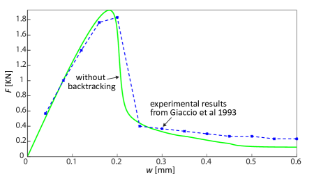
Figure 20: Example 6.4. $3d$-symmetric bending test. Load-displacement curve associated with the evolution of the approximate energetic solutions. For this case, standard application of the alternating minimization identifies the energetic solutions without resorting to the backtracking strategy.

$\begin{array}[]{cc}\includegraphics[width=211.26027pt]{Beam3dEnergVarWithWithoutBT3-vr1.pdf}&\includegraphics[width=211.26027pt]{Beam3dEnrgEstWithoutBT3-vr1.pdf}\\ (a)&(b)\end{array}$

Figure 21: Example 6.4. $3d$-symmetric bending test. Results for $\Delta w=10^{-3}\,\mathrm{mm}$. Evolution of: $(a)$ the total energy $\mathcal{E}(t_{n+1},\bm{U}_{n+1},\bm{A}_{n+1})+\sum_{i=0}^{n}\mathcal{D}(\bm{A}_{i},\bm{A}_{i+1})$ for $n=0,1,\ldots,N-1$ and $(b)$ of the total incremental energy $\mathcal{E}_{n+1}-\mathcal{E}_{n}+\mathcal{D}_{n,n+1}$, the lower bound $LB_{n,n+1}$ and the upper bound $UB_{n,n+1}$ which enter the two-sided energy estimate (5.6), $n=0,1,\ldots,N-1$. For this problem, standard application of the alternating minimization identifies the energetic solutions without resorting to the backtracking strategy.

$\begin{array}[]{ccc}\includegraphics[width=140.84256pt]{B3Dstp201.pdf}\includegraphics[width=14.08353pt]{LegendDamageMap3d.pdf}&\includegraphics[width=140.84256pt]{B3Dstp381.pdf}&\includegraphics[width=140.84256pt]{B3Dstp591.pdf}\\ \includegraphics[width=140.84256pt]{beamdamagemap3cropAI.pdf}&\includegraphics[width=140.84256pt]{beamdamagemap7cropAI.pdf}&\includegraphics[width=140.84256pt]{beamdamagemap17cropAI.pdf}\\ w=0.171\,\mathrm{mm}&w=0.291\,\mathrm{mm}&w=0.591\,\mathrm{mm}\end{array}$

Figure 22: Example 6.4. $3d$-symmetric bending test. Phase field distribution on the cross section $y=420\,\mathrm{mm}$ with correspondent $3d$ views of the phase-field isolevel lines. In the damage maps, the darkest colour corresponds to $\beta=1-\delta$ with $\delta=10^{-4}$ given that we are considering a partially damage profile, whereas the blue corresponds to solid material for which $\beta=0$.

7 Conclusions

In this paper we have proposed an algorithm that computes the solutions of the energetic formulation of an anisotropic phase-field model of quasi–brittle fracture characterized by a different behaviour at traction and compression and by a state dependent dissipation potential. Through the simulation of $2d$ and $3d$ benchmark problems, our results show that the standard procedure of simply solving the weak form of the Euler-Lagrange equations detects generally solutions that violate the modelling assumption of evolution via global minima of the discrete functionals which underpins the variational formulation of fracture and its corresponding energetic formulation. We have verified this assumption by checking an additional optimality condition of the global minimizers. Such condition has the form of a two–sided energy estimate and consists in checking that within each time step $[t_{n},\,t_{n+1}]$, $n=1,\ldots,N$, the sum of the variation of the stored energy and of the dissipation between the state of the system at the time instants $t_{n}$ and $t_{n+1}$ is bounded above and below. As an alternative and first approximation to the application of global optimization algorithms, which would not be viable in our case, given their high numerical complexity, we have designed a feasible numerical aproach that automatically enforces the meeting of the two-sided energetic estimates and allows the computation of improved energetic solutions consistent with the basic assumptions. The implementation of the energy estimates has been done within a backtracking strategy by which one goes back over past time steps when the estimates are violated, and restarts the simulation of the incremental problem with different initial condition for the phase-field variable. We noted, however, that there might be cases where the backtracking procedure is not activated, which occur especially in those situations where the lower energy bound is small and the two energy bounds are well apart from each other. This has occurred, for instance, in the $3d$ simulation of the symmetric bending beam whereas in the other cases, the check of the bounds has been determinant to find different energetic solutions which comply with the energetic bounds. In this case we cannot infer anything about the computed solution, though we believe, that, still within the field of application of methods of local optimization, a backtracking strategy based on sharper bounds would select more reliable energetic solutions. Finally, following the validation of the formulation to model crack in concrete, we believe that a better modelling of the cracking process upon different loading conditions can be obtained by including plasticity and cohesive effects, thus elaborating, for instance, the formulation advanced in [2, 3] where we account of what we have developed in our present work. This is part of an ongoing research.

References

- [1] Alessi R., Energetic formulation for rate-independent processes: Remarks on discontinuous evolutions with a simple example. Acta Mechanica 227 (2016) 2805-2829.
- [2] Alessi R., Marigo J.-J., Vidoli S., Gradient damage models coupled with plasticity: variational formulation and main properties. Mechanics of Materials 80 (2015) 351–367
- [3] Alessi R., Marigo J.-J., Maurini C., Vidoli S., Coupling damage and plasticity for a phase-field regularisation of brittle, cohesive and ductile fracture: one-dimensional examples. International Journal of Mechanical Sciences 149 (2018) 559–576
- [4] Almi S., Negri M., Analysis of staggered evolutions for nonlinear energies in phase-field fracture. Archive for Rational Mechanics and Analysis 236 (2020) 189–252.
- [5] Ambati M., Gerasimov T., De Lorenzis L., A review on phase-field models of brittle fracture and a new fast hybrid formulation. Computational Mechanics 55 (2015) 383–405.
- [6] Ambrosio L., Tortorelli V.M., Approximation of functionals depending on jumps by elliptic functionals via -convergence. Communications on Pure and Applied Mathematics 43 (1990) 999–1036.
- [7] Amor H., Marigo J.-J, Maurini C., Regularized formulation of the variational brittle fracture with unilateral contact: Numerical experiments. Journal of the Mechanics and Physics of Solids 57 (2009) 1209–1229.
- [8] ASTM E1820-20a, Standard Test Method for Measurement of Fracture Toughness, ASTM International, West Conshohocken, PA, 2020.
- [9] Bathe K., Finite Element Procedures. Prentice Hall, USA, 2nd Ed., 1996.
- [10] Benesova B., Global optimization numerical strategies for rate–independent processes. Journal of Global Optimization 50 (2011) 197–220.
- [11] Bertsekas D. P., Nonlinear Programming. Athena Scientific, USA, 3rd Ed., 2016.
- [12] Besson J., Cailletaud G., Chaboche J.-L., Forest S., Non-Linear Mechanics of Materials. Springer-Verlag, Berlin, 2010.
- [13] Blanchard P., Bruning E., Variational Methods in Mathematical Physics. Springer-Verlag, Berlin, 1992.
- [14] Bleyer J., Alessi R., Phase-field modeling of anisotropic brittle fracture including several damage mechanisms. Computer Methods in Applied Mechanics and Engineering 336 (2018) 213-23
- [15] Bourdin B., Numerical implementation of the variational formulation for quasi-static brittle fracture. Interfaces Free Boundaries 9 (2007) 411–430.
- [16] Bourdin B., Francfort G., Marigo J. J., Numerical experiments in revisited brittle fracture. Journal of the Mechanics and Physics of Solids 48 (2000) 797–826.
- [17] Bourdin B., Francfort G., Marigo J. J., The Variational Approach to Fracture. Springer, USA, 2008.
- [18] Bourdin B., Marigo J. J., Maurini C., Sicsic P., Morphogenesis and propagation of complex cracks induced by thermal shocks. Physical Review Letters 112 (2014) 014301.
- [19] Braides A., Local Minimization, Variational Evolution and Gamma-convergence. Lecture Notes in Mathematics 2094. Springer-Verlag, Switzerland, 2014.
- [20] Braides A., Dal Maso G., Garroni A., Variational formulation of softening phenomena in fracture mechanics: The one-dimensional case. Archive of Rational Mechanics and Analysis 146 (1999) 23–58.
- [21] Brun M. K., Wick T., Berre I., Nordbotten J. M., Radu F. A., An iterative staggered scheme for phase field brittle fracture propagation with stabilizing parameters. Computer Methods in Applied Mechanics and Engineering 361 (2020) 112752.
- [22] Carstensen C., Conti S., Orlando A., Mixed analytical-numerical relaxation in single-slip crystal plasticity. Continuum Mechanics & Thermodynamics 20 (2008) 275-301.
- [23] Chambolle A., Conti S., Francfort G., Approximation of a britlle fracture energy with a constraint of non-interpenetration, Archive of Rational Mechanics and Analysis 228 (2018) 867–889.
- [24] Ciarlet P. G., Introduction to Numerical Linear Algebra and Optimisation. Cambridge University Press, UK, 1989.
- [25] Conti S., Lenz M., Rumpf M., Hysteresis in magetic shape memory composites: Modeling and simulation. Journal of the Mechanics and Physics of Solids 89 (2016) 272–286.
- [26] Dacorogna B., Direct Methods in the Calculus of Variations Springer-Verlag, Berlin, 2nd Ed., 2008.
- [27] Dal Maso G., Toader R., A model for the quasistatic growth of brittle fractures: existence and approximation results. Archive of Rational Mechanics and Analysis 162 (2002) 101–135.
- [28] Dal Maso G., Toader R., A model for the quasistatic growth of brittle fractures based on local minimization. Mathematical Models and Methods in Applied Sciences 12 (2002) 1773–1799.
- [29] De Borst R., Verhoosel C.V., Gradient damage vs phase-field approaches for fracture: Similarities and differences. Computer Methods in Applied Mechanics and Engineering 312 (2016) 78–94.
- [30] DeLorenzis L., Gerasimov T., Numerical implementation of phase-field models of brittle fracture. In DeLorenzis L., Duster A. (eds), Modeling in Engineering Using Innovative Numerical Methods for Solids and Fluids, CISM 599, Springer, 2020.
- [31] Egger A., Pillai U., Agathos K., Kakouris E., et al., Discrete and phase field methods for linear elastic and fracture mechanics: A comparative study and state-of-art review. Applied Sciences 9 (2019) 2436.
- [32] Farrell P.E., Maurini C., Linear and nonlinear solvers for variational phase-field models of brittle fracture. International Journal for Numerical Methods in Engineering 109 (2017) 648–667.
- [33] Francfort G., Larsen C. J., Existence and convergence for quasistatic evolution in brittle fracture. Communications on Pure and Applied Mathematics 56 (2003) 1465–1500.
- [34] Francfort G., Marigo J.-J., Revisiting brittle fracture as an energy minimization problem. Journal of the Mechanics and Physics of Solids 46 (1998) 1319–1342.
- [35] Freddi F., Royer-Carfagni G., Regularized variational theories of fracture: A unified approach. Journal of the Mechanics and Physics of Solids 58 (2010) 1154–1174.
- [36] Frémond M., Non–Smooth Thermomechanics. Springer-Verlag, Berlin, 2002.
- [37] Frémond M., Virtual Work and Shape Change in Solid Mechanics. Springer-Verlag, Berlin, 2017.
- [38] Frémond M., Nedjar B., Damage, gradient of damage and principle of virtual power. International Journal of Solids & Structures 33 (1996) 1083–1103.
- [39] Gerasimov T., DeLorenzis L., A line search assisted monolithic approach for phase-field computing of brittle fracture. Computer Methods in Applied Mechanics and Engineering 312 (2016) 273–303.
- [40] Gerasimov T., DeLorenzis L., On penalization in variational phase-field models of brittle fracture. Computer Methods in Applied Mechanics and Engineering 354 (2019) 990–1026.
- [41] Giaccio G., Rocco C., Zerbino R., The fracture energy () of high-strength concretes. Materials and Structures 26 (1993) 381–386.
- [42] Giacomini A., Ambrosio-Tortorelli approximation of quasi-static evolution of brittle fractures. Calculus of Variations and Partial Differential Equations 22 (2005) 129–172.
- [43] Glowinski R., Lions J. L., Trèmoliéres R., Numerical Analysis of Variational Inequalities – Studies in Mathematics and Its Applications. North-Holland Publication, Netherlands, 1981.
- [44] Griffith A. A., The phenomena of rupture and flow in solids. Philosophical Transactions of the Royal Society A 221 (1921) 163–198.
- [45] Gurtin M.E., An Introduction to Continuum Mechanics. Academic Press, USA, 1970.
- [46] Han W., Reddy B. D., Plasticity: Mathematical Theory and Numerical Analysis. Springer-Verlag, USA, 2nd Ed., 2013.
- [47] Kachanov L. M., Time of the rupture process under creep conditions. Izvestiia Akademii Nauk SSSR, 8 (1958) 26-31.
- [48] Kirkesaether brun M., Wick T., Berre I., Nordbotten J. M., Radu F. A., An iterative staggered scheme for phase field brittle fracture propagation with stabilizing parameters. Computer Methods in Applied Mechanics and Engineering 361 (2020) 112752.
- [49] Jost J., Li-Jost X., Calculus of Variations. Cambridge University Press, New York, 1998.
- [50] Knees D., Negri M., Convergence of alternate minimization schemes for phase-field fracture and damage Mathematical Models and Methods in Applied Sciences 27 (2017) 1743–1794.
- [51] Lancioni G., Royer-Carfagni G., The variational approach to fracture mechanics: A practical application to the French Pantheon in Paris. Journal of Elasticity 95 (2009) 1–30.
- [52] Lemaitre J., Chaboche J.-L., Mechanics of Solid Materials. Cambridge University Press, UK, 1998.
- [53] Li T., Gradient-damage modeling of dynamic brittle fracture: Variational principles and numerical simulations. PhD thesis, Université Paris 13, Paris, France, 2016.
- [54] Lorentz E., Andrieux S., A variational formulation for nonlocal damage models. International Journal of Plasticity 15 (1999) 119–138.
- [55] Lorentz E., Andrieux S., Analysis of non-local models through energetic formulations. International Journal Solids & Structures 40 (2003) 2905–2936.
- [56] Lorentz E., Cuvilliez S., Kazymyrenko K., Convergence of a gradient damage model toward a cohesive zone model. Comptes Rendus Mécanique 339 (2011) 20–26.
- [57] Luege M., Orlando A., Almenar M., Pilotta E., An energetic formulation of a gradient damage model for concrete and its numerical implementation. International Journal of Solids & Structures 155 (2018) 160–184.
- [58] Marigo J.-J., Initiation of cracks in Griffith’s theory: An argument of continuity in favor of global minimization. Journal of Nonlinear Science 20 (2010) 831–868.
- [59] Marigo J.-J., Maurini C., Pham K., An overview of the modelling of fracture by gradient damage models. Meccanica 51 (2016) 3107–3128.
- [60] Mesgarnejad A., Bourdin B., Khonsari M. M., Validation simulations for the variational approach to fracture. Computer Methods in Applied Mechanics and Engineering 290 (2015) 420–437.
- [61] Miehe C., A multi–field incremental variational framework for gradient–extended standard dissipative solids. Journal of the Mechanics and Physics of Solids 59 (2011) 898–923.
- [62] Miehe C., Hofacker M., Welschinger F., A phase field model for rate-independent crack propagation: Robust algorithmic implementation based on operator splits. Computer Methods in Applied Mechanics and Engineering 199 (2010) 2765–2778.
- [63] Miehe C., Welschinger F., Hofacker M., Thermodynamically consistent phase-field models of fracture: Variational principles and multi-field FE implementations. International Journal for Numerical Methods in Engineering 83 (2010) 1273–1311.
- [64] Mielke A., Roubíček T., Rate-independent damage processes in nonlinear elasticity. Mathematical Models and Methods in Applied Sciences 16 (2006) 177–209.
- [65] Mielke A., Roubíček T., Rate-Independent Systems. Theory and Application. Springer-Verlag, Berlin, 2015.
- [66] Mielke A., Roubicek T., Zeman J., Complete damage in elastic and viscoelastic media and its energetics. Computer Methods in Applied Mechanics and Engineering 199 (2010) 1242–1253.
- [67] Moës N., Dolbow J., Belytschko T., A finite element method for crack growth without remeshing International Journal for Numerical Methods in Engineering 46 (1999) 131–150.
- [68] Most T., Bucher C., Energy–based simulation of concrete cracking using an improved mixed–mode cohesive crack model within a meshless discretization. International Journal for Numerical and Analytical Methods in Geomechanics 31 (2007) 285–305.
- [69] Nguyen Q. S., Stability and Nonlinear Solid Mechanics. John Wiley & Sons, Ltd, Chichester, 2000.
- [70] Nguyen Q. S., Quasi-static responses and variational principles in gradient plasticity. Journal of the Mechanics and Physics of Solids 97 (2016) 156–167.
- [71] Nguyen T.-T., Yvonnet J., Waldmann D., He Q.-C., Implementation of a new strain split to model unilateral contact within the phase field method. International Journal for Numerical Methods in Engineering 121 (2020) 4717–4733.
- [72] Pham K., Amor H., Marigo J. J., Maurini C., Gradient damage models and their use to approximate brittle fracture. International Journal of Damage Mechanics 20 (2011) 618–652.
- [73] Pham K., Marigo J. J., Maurini C., The issues of the uniqueness and the stability of the homogeneous response in uniaxial tests with gradient damage models. Journal of the Mechanics and Physics of Solids 59 (2011) 1163–1190.
- [74] Quarteroni A., Numerical Models for Differential Problems. Springer Verlag, Milan, 2017.
- [75] RILEM 50-FMC Committee (Fracture Mechanics of Concrete), Determination of the fracture energy of mortar and concrete by means of three–point bend test on notched beams, Materials and Structures 18 (1985) 285–290.
- [76] Roubicek T., Kruzik M., Zeman J., Delamination and adhesive contact models and their mathematical analysis and numerical treatment (chap. 9). In: Mathematical Methods and Models in Composites, V. Mantic (Ed.), World Scientific Press, 2013, 349–400.
- [77] Stefanelli U., A variational characterization of rate-independent evolution. Mathematische Nachrichten 282 (2009) 1492–1512.
- [78] Tanné E., Li T., Bourdin B., Marigo J.-J., Maurini C., Crack nucleation in variational phase-field models of brittle fracture. Journal of the Mechanics and Physics of Solids 110 (2018) 80-99
- [79] Thomas M., Mielke A., Damage of nonlinearly elastic materials at small strain - existence and regularity results. ZAMM Z. Angew. Math. Mech. 90 (2010) 88–112.
- [80] Ulloa J., Rodriguez P., Samaniego C., Samaniego E., Phase-field modeling of fracture for quasi-brittle materials. Underground Space 4 (2019) 10–21.
- [81] Wick T., Modified Newton methods for solving fully monolithic phase-field quasi–static brittle fracture propagation. Computer Methods in Applied Mechanics and Engineering 325 (2017) 577–611.
- [82] Winkler B., Traglastuntersuchungen von unbewehrten und bewehrten Betonstrukturen auf der Grundlage eines objektiven Werkstoffgesetzes für Beton. University Press, Innsbruck, 2001.
- [83] Wu J.-Y., A unified phase-field theory for the mechanics of damage and quasi–brittle failure. Journal of the Mechanis and Physics of Solids 103 (2017) 72–99.
- [84] Wu J.-Y., Nguyen V. P., Nguyen C. T., Sutula D., Sinaie S., Bordas S., Phase-field modeling of fracture. Advances in Applied Mechanics 53 (2020) In Press, Corrected Proof.
- [85] Zeman J., Gruber P., Numerical approach to a rate-independent model of decohesion in laminated composites, J. Chleboun, P. Prikryl, K. Segeth and J. Sistek (Eds.): Programs and Algorithms of Numerical Mathematics, Proceedings of Seminar Dolni Maxov, June 6–11, 2010. Institute of Mathematics AS CR, Prague, 2010, 239–250.