Several new product identities in relation to two-variable Rogers–Ramanujan type sums and mock theta functions
Abstract.
Product identities in two variables expand infinite products as infinite sums, which are linear combinations of theta functions; famous examples include Jacobi’s triple product identity, Watson’s quintuple identity, and Hirschhorn’s septuple identity. We view these series expansions as representations in canonical bases of certain vector spaces of quasiperiodic meromorphic functions (related to sections of line and vector bundles), and find new identities for two nonuple products, an undecuple product, and several two-variable Rogers–Ramanujan type sums. Our main theorem explains a correspondence between the septuple product identity and the two original Rogers–Ramanujan identities, involving two-variable analogues of fifth-order mock theta functions. We also prove a similar correspondence between an octuple product identity of Ewell and two simpler variations of the Rogers–Ramanujan identities, which is related to third-order mock theta functions, and conjecture other occurrences of this phenomenon. As applications, we specialize our results to obtain identities for quotients of generalized Dedekind eta functions and mock theta functions.
1. Introduction
Fix with , and let . Denote , , , and (the standard notations have a subscript of , which we drop for brevity; this will be helpful in identities like 1.4). Then Jacobi’s triple product identity [13, p. 10] reads
| (1.1) |
As functions of , both sides of 1.1 converge absolutely and locally uniformly to entire -periodic functions, and satisfy the -quasiperiodicity ; in geometric language, is a section of a certain holomorphic line bundle over the complex torus . This observation already proves 1.1 up to a factor depending only on , since the space can be shown to be one-dimensional over by identifying Fourier coefficients (here, denotes the space of entire functions with period ). More generally, if is open, connected and closed under -translation, and , then the space
can be shown to be finite-dimensional over for various choices of and . In particular, given a positive integer and a nonzero , the space has a canonical basis consisting of the theta functions
where varies in any complete residue system modulo (we introduce this notation because it will admit a natural generalization to other functions of the form ). Many infinite products can be designed to live in such spaces (see Table 1, ), so it is natural to look for their representations in a canonical basis thereof; e.g., 1.1 states that . Similarly, the quintuple [49] and septuple [35, 20, 27, 24] product identities respectively state that
| (1.2) | ||||
| (1.3) |
In this paper, we prove several new product identities pertaining to more general spaces , and study their connection to two-variable Rogers–Ramanujan type sums [43]; as applications, we deduce a few one-variable identities of generalized eta functions [52] and mock theta functions [39, 9]. The latter were introduced by Ramanujan in his last letter to Hardy [39], and are modernly understood as holomorphic parts of harmonic weak Maass forms [15]. We will find that the fifth-order mock theta functions are intimately related to the canonical basis vectors of (where ), while the third-order ones are similarly connected to the space .
For a start, in Section 4.1 we continue the sequence of identities 1.1, 1.2, 1.3 in a natural way, with two nonuple product identities and an undecuple identity; we state the first of these below.
Proposition 1.1 (First nonuple product identity).
As an identity of functions in ,
| (1.4) |
While is -dimensional for , we have for ; this will lead to identities for quotients of double infinite products , in Proposition 3.26. Passing to spaces such as , which is two-dimensional and corresponds to a meromorphic line bundle, we begin to encounter Rogers–Ramanujan type sums. In fact, the two renowned Rogers–Ramanujan identities [32, p. 290],
| (1.5) |
where , are together equivalent to the following new product identity.
Proposition 1.2 (Two-variable statement of 1.5).
In , one has
| (1.6) |
where for , is the unique function in whose Fourier expansion in has coefficient of equal to , for .
Remark.
The functions can be expressed as explicit series in (see Corollary 3.18), and can then be meromorphically continued to ; their poles must cancel out in the right-hand side of 1.6 since the left-hand side is entire. In fact, while . Also, the Rogers–Ramanujan identities in 1.5 follow from the second equality in 1.6 by identifying coefficients of and . In fact, identifying coefficients of for leads to the so-called -versions of the Rogers–Ramanujan identities, involving (see, e.g., [26, (3.5)]).
Much of the work in this paper is motivated by a visible connection between Proposition 1.2 and the septuple identity: the basis representations in 1.3 and 1.6 have the same -coefficients, up to a sign. This suggests the more difficult result that sums of canonical basis vectors of are proportional to the canonical basis vectors of , which is our main theorem:
Theorem 1.3 (Septuple identity vs. Rogers–Ramanujan).
For , one has
as an identity of meromorphic functions of (where ). The left-hand side above equals minus the ratio of the septuple product in 1.3 to the product in Proposition 1.2.
In particular, under Theorem 1.3, the septuple identity and 1.6 are equivalent. Remarkably, an analogous correspondence arises between the octuple product identity of Ewell [23] (given in an equivalent form in this paper’s Proposition 4.7) and a variation of 1.6, given in Proposition 5.4.
Theorem 1.4 (Octuple identity vs. Rogers–Ramanujan variation).
For , one has
as an identity of meromorphic functions of (where ). The left-hand side above equals minus the ratio of the octuple product in 4.13 to the product in Proposition 5.4. Here, are defined analogously to in Proposition 1.2.
One can also specialize our two-variable results at particular values of , to produce one-variable identities of modular forms and mock theta functions; we further mention one corollary about each, proven using Proposition 1.1 and Theorem 1.3 respectively. First, denote the Dedekind eta function and the generalized Dedekind eta functions of level (following [52, Corollary 2]) by
| (1.7) |
where , , and the level must be specified a priori (the generalized eta functions should not be confused with the Eisenstein series ). It should not be surprising, based on 1.7, that specializing product identities at recovers identities for products and quotients of eta functions; what is more intriguing is the simplicity and symmetrical structure of these identities (which are related to their behavior under modular transformations; see Section 4.2 for more details and examples). Corollary 1.5 provides one such result.
Corollary 1.5 (Eta quotient polynomial).
For , let denote the generalized eta functions of level . Then one has the polynomial factorization
Our second corollary involves four of Ramanujan’s famous fifth-order mock theta functions [48, 9]:
| (1.8) |
Corollary 1.6 (Fifth-order mock theta sums).
For , one has
Remark.
Corollary 1.6 follows from Theorem 1.3 by taking , and Theorem 1.4 is similarly related to third-order mock theta functions; we also obtain individual identities for in Proposition 5.15. More difficult identities for and are given by Ramanujan’s famous mock theta conjectures [9], proven by Hickerson [33] and more recently by Folsom using Maass forms [25].
The table below provides short -expansions of the relevant series in Corollary 1.6.
Finally, while proving Theorems 1.3 and 1.4, we find it useful to work with three different bases of and to determine the corresponding change-of-basis matrices; their entries turn out to be two-variable Rogers–Ramanujan type sums. We gather the resulting matrix identities in Theorem 5.11, but for now we only mention a particular case which is closely related to Theorem 1.3:
Proposition 1.7 (Two-variable determinant identity).
For with , one has
We conclude the introduction with an open question that arises from our work:
Question 1.
As noted by Andrews, Schilling and Warnaar [4, (5.2)], the Rogers–Ramanujan products and are characters of a certain algebra, which they denote by . We remarked that these products coincide with the -coefficients of the canonical basis vectors in the septuple identity 1.3, and explained this correspondence through Theorem 1.3. A similar phenomenon occurs for the octuple (Proposition 4.7) and nonuple (Proposition 1.1) identities:
| Algebra | Product identity | Rog.–Ram. type id. | 2-Var. generaliz. | Correspondence |
|---|---|---|---|---|
| Septuple, 1.3 | 1.5 | Proposition 1.2 | Theorem 1.3 | |
| Octuple, 4.13 | 5.8 | Proposition 5.4 | Theorem 1.4 | |
| Nonuple, 1.4 | [21, Theorem 1.1] | (Open question) | (Open question) |
Indeed, the -coefficients in the right-hand side of the nonuple identity 1.4 coincide with the 4 characters of the algebra (up to factors of ), and [4, Theorem 5.2] gives Rogers–Ramanujan identities for 3 out of these characters (see also [47]); the more recent work of Corteel and Welsh also provides the fourth identity [21, Theorem 1.1]. Can one complete the bottom row of the table above with an analogue of Theorem 1.3, leading to a new proof of Theorem 1.1 from [21], and possibly to applications on higher-order mock theta functions?
Remark.
There is also a product identity whose -coefficients are the characters of , for any relatively prime positive integers such that is odd; see our Corollary 4.3. These might be connected as in Question 1 to the Andrews–Gordon identities [7, Theorem 7.8], which generalize 1.5; Theorem 1.3 would correspond to the case . As pointed out by Professor S. Ole Warnaar (personal communication), the analogue of Proposition 1.2 in this case could be a summation of variants of the Andrews–Gordon identities as in [11, (3.21)]; the difficulty lies in relating such a summation to an infinite product in a suitable space.
2. Overview and Notation
2.1. Methods
Given an entire -periodic function , there are two main ways to construct a function with a -type quasiperiodicity from scratch: the expressions
| (2.1) |
are, if well-defined, quasiperiodic with . Given that many of the spaces are finite-dimensional (as we prove in Section 3.1), identities relating infinite products to infinite sums as above are bound to arise. Taking and , one recovers and as the product, respectively the sum in 2.1; the same sum leads to formulae for other basis vectors , as we show in Section 3.2.
The constructions in 2.1 also correspond to two ways to produce new functions in from old ones. Firstly, the product of a function in and a function in is a function in ; for instance, . Going further, the product of two basis vectors and (where , , ) is an element of , so we must have
| (2.2) |
for some M-coefficients . Closely related identities were noted by various authors in different forms [20, 2, 51]; we formulate a generalization of 2.2 in Lemma 4.1, and use it together with the triple and quintuple product identities to deduce the nonuple and undecuple identities.
In a similar spirit, twisting the th term in a series as in 2.1 by a factor of (for suitable functions with period ) should preserve the quasiperiodicity at . In particular, by twisting the series defining , we should be able to write (when well-defined)
| (2.3) |
for some W-coefficients , provided that the left-hand side is entire. We identify a class of such identities in Lemma 5.6, leading to one method of proof for Theorems 1.3, 1.4 and 5.11.
2.2. Layout of paper
In Section 3, we formally define and study a generalization of the vector spaces , then give a few applications including the triple and quintuple product identities. Section 4 states and proves the nonuple and undecuple product identities alongside other similar results, and then uses them to produce identities of generalized eta functions such as Corollary 1.5. Finally, Section 5 deals with applications on Rogers–Ramanujan type sums, including the proofs of Propositions 1.2 and 1.7, Theorems 1.3 and 1.4, and results on mock theta functions such as Corollary 1.6. The relationships between our main results are collected in Figure 1.
In Figure 1, if an arrow has multiple tails, the meaning is that all of the tails collectively imply each of the heads. If an arrow has two-sided heads (and no tails), then the heads facing in one direction are together equivalent to the heads facing in the other direction. So for instance, by going from left to right through Theorem 5.2 (which is ultimately equivalent to Theorem 1.3), one obtains a new proof of four Rogers–Ramanujan type identities from Slater’s famous list [44, (94),(96),(98),(99)]. Going backwards, one has a proof that these four identities of Slater imply the Rogers–Ramanujan identities 1.5 and several mock theta identities. Also, some nodes in Figure 1 are colored with a lighter green to indicate that the results therein are only partly new, or that closely related results have appeared in literature, albeit in different formulations.
2.3. Notation
Denote , , . Throughout the paper we keep fixed and let vary, and write , and for . Given a domain (an open connected subset of ), denote by the space of all holomorphic functions on ; if is closed under -translation, denote by the space of all functions in with period . Given and , define the linear maps and by
which are a translation and a scaling of the function’s argument. Since , these also induce natural maps and when is -invariant. Given such and a meromorphic function on , , we denote
| (2.4) | ||||
| (2.5) |
where and are understood as equalities of meromorphic functions. We regard and as complex vector spaces; this generalizes the notation used in Section 1.
Next, we extend the notation from Section 1 to all by setting
| (2.6) |
The point of this convention is to extend the relation to all . As before, we write , implying that . The double product is commonly referred to as a modified theta function, and often found in literature as [20] or [28, (11.2.1)]. It shortly follows that for any , a symmetry which is crucial to most proofs of product identities. But more surprisingly, if for and such that , a short computation left to the reader shows that also satisfies a simple -type symmetry recorded in Table 1; these explain why the basis vectors pair up in the quintuple, septuple and nonuple identities.
| Function | |||||
| -Space | |||||
| -Space | – | – |
In taking products of such functions it is fairly easy to bookkeep the spaces and involved, by simply multiplying the factors therein. One can think of these factors as units of measurement, which are multiplied in the left-hand sides of product identities (such as 1.1–1.4), and which must be homogeneous in the sums from the right-hand-sides. For completion, we also state three easy manipulations of infinite products, which may be used implicitly throughout the paper: for any positive integer , one has
where ranges over the th complex roots of unity.
The notation will be used for certain canonical elements of , generalizing the functions from Section 1; see Proposition 3.13. By abuse of notation we may write an expression depending on in place of , e.g. when . As a word of caution, this notation does not obey the rule of substitution in , so for instance ; the expression before the semicolon indicates a -quasiperiodicity factor (e.g., ), not an argument of the function.
Given a nonempty open horizontal strip , a function and , write
for any (the choice of is irrelevant by contour-shifting). The Fourier series of converges absolutely and locally uniformly in , so in particular we can multiply the Fourier series of two such functions using the natural sum rearrangements. If is a Laurent polynomial in , we write for its degree in , i.e. the largest such that .
Finally, we write for and , and for the truth value of a proposition (e.g., equals whenever , and otherwise). We leave the notations concerning generalized eta functions and mock theta functions to Sections 4.2 and 5.3.
3. Structure of the relevant function spaces and first applications
3.1. Dimensionality bounds
We start by generalizing the spaces .
Definition 3.1 (Extended quasiperiodic function spaces).
Let be a -invariant domain, a positive integer, and meromorphic functions on (i.e., on with period ), with (i.e., is not the zero function). We define the complex vector space
where the equality holds as an identity of meromorphic functions on . More generally, given an matrix whose entries are meromorphic functions on such that , let
where the equality holds as an identity of meromorphic functions on , and as before. In particular, we have a linear bijection
While much of this paper is concerned with the spaces (in fact, Section 4 only works with ), we will encounter more general spaces and in Section 5.
Example 3.2 (Two-variable Rogers–Ramanujan fraction).
Consider the entire -periodic function (this is from [41, p. 329]). A short computation shows that
so and thus . This vector space turns out to be one-dimensional, which can be used to prove an identity due to Rogers generalizing the Rogers–Ramanujan identities in 1.5; see Proposition 5.1. By iterating this functional equation in matrix form, one can also recover the Rogers–Ramanujan continued fraction identity [41, p. 328 (4)],
where the infinite product of matrices above is computed from the left to the right.
Example 3.3 (Line bundles and theta functions).
Take and in Definition 3.1, and let be any invertible function in . For and , define as if , and as otherwise. Then form a system of multipliers for the lattice , meaning that they are holomorphic invertible and they satisfy the cocycle condition (see, for example, [10, §2.3]). Such a system induces a holomorphic line bundle over , where acts on by ; a section of this line bundle has the form
where satisfies , and this reduces to by our choice of . Hence the sections of are canonically identified with the elements of , and these are called the theta functions associated to . Canonical examples are Jacobi’s theta functions (see [36] or [50, p. 464]), and more generally the functions .
While the triple, quintuple, septuple, etc. products all lie in such vector spaces induced by invertible functions , allowing to have zeros at the cost of reducing the domain of holomorphicity of is essential for stating and proving results like Proposition 1.2, Theorem 1.3 or Theorem 1.4. If contains a horizontal strip of length (thus a copy of ), the more general spaces correspond similarly to meromorphic line bundles, while the spaces (where is an matrix) correspond to vector bundles of rank (of the form where ) and generalized (or non-abelian) theta functions (see [10, §6.2] or [31]). It can be helpful, however, to consider smaller domains not containing any copy of , as we illustrate Proposition 3.26. For the reader familiar with this language, the properties in the following lemma will come naturally; e.g., Lemma 3.4.(iii) is motivated by the fact that multiplying a vector bundle by a line bundle yields back a vector bundle of the same rank.
Lemma 3.4 (Basic facts about ).
Let and be as in Definition 3.1.
-
(i).
If is another -invariant domain and , then , where a function in is uniquely identified with its restriction to .
-
(ii).
For , one has .
-
(iii).
Letting , one has ; so if , then . Also, if has no zeros in , then .
-
(iv).
If , and , then
-
(v).
If contains an open horizontal strip of width , then has a meromorphic continuation to all of , which still satisfies .
-
(vi).
If contains an open horizontal strip of width , and , then extends to an elliptic function on with periods .
Proof.
Statements (i) and (ii) are immediate, while (iii) and (iv) follow by repeatedly applying (ii) for . For (v), let be an open horizontal strip of width ; then we can iteratively define on the strips for , and
on for ; note that is well-defined on by the uniqueness of meromorphic continuation. Finally, (vi) follows from (v) applied to and , and then (iii) applied for (one has , and so ). ∎
Remark.
By Lemma 3.4.(v), we can treat the elements of as meromorphic functions on if is wide enough; the same is true in more general spaces , where the continuation requires inverting the matrix . The restriction of holomorphicity on , however, will be crucial.
Example 3.5 (Spaces given by constants).
Suppose a domain contains a horizontal strip of length . Note that .
The proof of Lemma 3.4.(ii) then shows that any function can be continued to an entire elliptic function on , thus a constant. More generally, if is any nonzero constant, then for , considering the Fourier series of in yields
for any . So if for some , we find that is one-dimensional, spanned by ; otherwise, . We give a more general upper bound for in Proposition 3.6.
Proposition 3.6 (Upper bounds for ).
Let be complex polynomials in with and , and let . For , take . Suppose is a -invariant domain, containing an open horizontal strip of width . Letting , the following hold true.
-
(i).
One has .
-
(ii).
For , denote . Assume additionally that ,
Then one has , with equality iff , such that
In this case, is a (uniquely determined) basis of .
Example 3.7.
For , and , part (i) implies that whenever contains a horizontal strip of width . If , then in part (ii) we have , so any choice of yields . This recovers Example 3.5.
Example 3.8.
For , and , we have . Hence using in Proposition 3.6.(ii), we find that . In Example 3.2 we found a nonzero element of this space, so it must be the unique such function up to scalars.
Proof of Proposition 3.6.
For , we have and thus . Taking the Fourier series in then yields
which rearranges (by subtracting the right side from the left side and swapping sums) to
| (3.1) |
If , we find that whenever . So (ii) holds trivially since if all , we must have . For statement (i), note that one can have for at most values of , say among , since is a nonzero polynomial in of degree . Hence injects linearly into a subspace of by the map , proving .
Now assume that . When , 3.1 implies that is a linear function of . Similarly, when , is a linear function of . Hence under the assumption of (ii), injects linearly into by , proving that with equality iff each standard basis vector of is attained by this injection; the preimages of these vectors correspond to .
To prove (i), note as before that and can each be zero for at most values of (since is also a polynomial in of degree , which is not constantly by the definition of ). Say that has zeros only if , and let be large enough such that for all . Then by our previous reasoning, injects linearly into by , proving . ∎
Remark.
The bound in Proposition 3.6.(i) may be sharpened by determining the zeros of and in particular cases. Also, the linear relation in 3.1 gives a formula for the Fourier coefficients (for and ) in terms of finite matrix products; however, applications will require alternative formulae for , which we give in Section 3.2.
It is now convenient to briefly study the relationship between the and spaces; recall 2.5.
Lemma 3.9 (Basic facts about ).
Let be a -invariant domain and be meromorphic functions on .
-
(i).
If and , then .
-
(ii).
If and , then one has wherever defined.
-
(iii).
If and , then wherever defined,
Proof.
Statement (i) is clear, and (ii) follows by iterating the functional equation of any with ; note that having on a nonempty open set extends to everywhere. For (iii), let , and use these two symmetries of to obtain
as an identity of meromorphic functions in . Since this is a nonempty open set and is not the zero function, we can cancel and multiply by to obtain the desired claim (note that as meromorphic functions by (ii)). ∎
Remark.
A choice of meromorphic functions , which satisfy the conditions in Lemma 3.9.(ii)-(iii) is given by and , for . These come up in the next result.
Proposition 3.10 (Spaces given by monomials).
Let be any integer, and be a -invariant domain containing an open horizontal strip of width .
-
(i)
For any (which may depend on the fixed ), one has
Moreover, for , any has exactly zeros (counting multiplicities) in every fundamental region , for .
-
(ii)
For and ,
(3.2) So for , one obtains and . Moreover, all elements of have common zeros at:
Remark.
Proof.
For part (i), case was settled in Example 3.5. If , suppose that , and let . Then as in 3.1 we have for all . Fixing a nonzero Fourier coefficient , we find inductively that grows on the order of , which contradicts the convergence of the Fourier series of anywhere since .
Now suppose that . Take , and in Proposition 3.6, and consider . We have and for all , so Proposition 3.6.(ii) yields that , with equality iff there exist such that
| (3.3) |
where the Fourier series are taken in . Such functions are the canonical basis vectors from Section 1,
given by locally uniformly convergent Fourier series in . Thus these are entire -periodic functions satisfying and 3.3, proving that . In fact, for any , has nonzero Fourier coefficients only at multiples of plus , so the functions give a basis of for any complete residue system modulo . Since we have by Lemma 3.4.(i), the equality of dimensions forces an equality of vector spaces; i.e. each function in can be holomorphically continued to .
Concerning the claim about zeros in (i), the case is immediate since then can only be a scalar multiple of for some . For , note that has zeros whenever for , thus exactly zeros in any fundamental region as in part (i). Since the ratio of any two nonzero functions in is an elliptic function (by Lemma 3.4.(vi)), the same is true for any .
For part (ii), the case is easily verified, so take . We can also assume WLOG that due to the linear bijection given by multiplication by ,
which also preserves canonical bases and zeros; note that . A quick computation shows that for (using that ), and so as anticipated in Table 1. In fact, we claim that the functions
| (3.4) |
span . Indeed, any can be written as and , by identifying Fourier coefficients in two basis representations of . Hence
Assuming additionally that , we find that by identifying Fourier series, and thus is spanned by the sums in 3.4. Since has null Fourier coefficients anywhere else other than at multiples of plus-minus , it is clear that the vectors in 3.4 are linearly independent provided that they are nonzero. But to have we would need in particular that , so . Treating these two cases separately leads to the two terms subtracted from in 3.2. For one has , so for the right choices of one can force an equality of vector spaces , proving the claimed inclusions.
Finally, for the statement about common zeros in (ii), consider the maps
where we used that and . These are injective linear maps of vector spaces of equal finite dimensions by 3.2 (e.g., for the first map both spaces have dimension ). Thus the three maps above are bijections, and determining the zeros of , and completes our proof. ∎
Corollary 3.11.
For with , the map
which divides by , is a bijection of -dimensional vector spaces. If is odd,
give more such bijections by multiplicative factors.
Proposition 3.12 (Spaces given by polynomials).
Suppose is a Laurent polynomial in with , such that has no zeros in . Then one has
and if , equality is reached in the right side if and only if is a monomial in . Moreover, any nonzero has exactly zeros (counting multiplicity) in any fundamental region , for .
Proof.
Write , where and is a polynomial in with free coefficient . Then consider the function
where the product converges locally uniformly in (given that converges); note that is designed to satisfy , hence . Moreover, since is nonzero on , each is nonzero on , so is nonzero on by standard properties of infinite products, and thus . Applying Lemma 3.4.(iii) twice, we find that multiplication by induces a bijective linear map
| (3.5) |
proving by Proposition 3.10. By Lemma 3.4.(i), this immediately implies that . Now say is not a monomial in , so it must have a zero , which results in a zero of . For , consider the product
Then has zeros precisely when for some , i.e. when for some and a fixed . Hence iff for some , which implies that and have no common zeros when . So assuming , there is some with , which implies that
This settles the equality case of (together with Proposition 3.10.(i)). The statement about zeros in fundamental regions of follows from the analogous statement in Proposition 3.10.(i) and the bijection in 3.5 (since has no zeros in ). ∎
Remark.
Combining Corollary 3.11 with the inclusion from Proposition 3.10, and the map in 3.5, we obtain bijections by multiplicative factors
where we used that and by 1.1 and 1.2 with adequate substitutions. What is special about the two resulting bijections (following the top and the bottom maps above) is that they preserve canonical bases: go to by the top chain of maps, while go to by the bottom one. This is the content of our main results in Theorems 1.3 and 1.4.
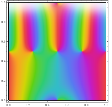
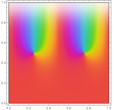
As predicted by Proposition 3.10.(i), has five zeros in the fundamental region . Three of these zeros, at , correspond to the zeros of and are eliminated by the bijection in Corollary 3.11; the remaining two nontrivial zeros coincide with the zeros of , as seen in Figure 2. For , the nontrivial zeros lie approximately and ; note that they sum up to since has a symmetry by a nonzero multiplicative factor at (by combining -periodicity with the symmetries from ).
3.2. Canonical basis vectors
We are now ready to define the promised generalization of the functions , and from Section 1 (and to show in particular that the latter two functions are well-defined).
Proposition 3.13 (Canonical basis).
Let be a polynomial in with , such that has no zeros in , and . Then has a canonical basis uniquely determined by
Proof.
Proposition 3.12 implies that , so we aim to apply the ‘only if’ part of the equality case in Proposition 3.6.(ii). We have and , so for all ,
Our assumptions imply that for all , and for all . Hence using , the conditions of Proposition 3.6.(ii) are fulfilled. ∎
Remark.
In the proof of Proposition 3.12, dividing the canonical basis of by yields a basis of , but this usually differs from the canonical basis (when well-defined); in fact, computing the relationship between these two bases is one of the main difficulties in proving Theorems 1.3 and 1.4. The advantage of expressing product identities in terms of the canonical basis is that for any , by identifying Fourier coefficients one can write
| (3.6) |
and the coefficients may be objects of interest (in Proposition 5.4 for example, they are the two Rogers–Ramanujan series from 1.5). In particular, if is a second-degree polynomial in with no zeros in and , Propositions 3.12 and 3.13 imply that and , with a basis . So if we are given an entire function , it must be unique up to a scalar, and it is natural to express it as in 3.6; this is the subject of Proposition 1.2 for .
Example 3.14.
For and , is a well-defined holomorphic function in by Proposition 3.12. By Lemma 3.4.(v), it can be continued meromorphically to , with simple poles at for with ; these poles are cancelled when multiplying by , as expected since we know is entire. Using 1.1, 1.2, and our main result in Theorem 1.3, one can easily compute the residues of these functions at the periodic poles ; up to a factor of , these are
which is consistent with the pole cancellation in Proposition 1.2. One can also verify this numerically as an identity of -series: expand in and write
since has the Fourier series in , and as (note that converges absolutely for , i.e. ).
| 11 | ||||||||||||||||||||||||
|---|---|---|---|---|---|---|---|---|---|---|---|---|---|---|---|---|---|---|---|---|---|---|---|---|
| 10 | ||||||||||||||||||||||||
| 9 | -1 | -1 | -1 | |||||||||||||||||||||
| 8 | 1 | 1 | 1 | 2 | 1 | 2 | 1 | |||||||||||||||||
| 7 | -1 | -1 | -1 | -1 | -1 | -1 | -1 | -1 | ||||||||||||||||
| 6 | 1 | 1 | 1 | 1 | 1 | |||||||||||||||||||
| 5 | -1 | -1 | -1 | |||||||||||||||||||||
| 4 | 1 | 1 | ||||||||||||||||||||||
| 3 | -1 | |||||||||||||||||||||||
| 2 | 1 | |||||||||||||||||||||||
| 1 | ||||||||||||||||||||||||
| 0 | 1 | |||||||||||||||||||||||
| -1 | 1 | |||||||||||||||||||||||
| -2 | 1 | 1 | ||||||||||||||||||||||
| -3 | 1 | 1 | 1 | |||||||||||||||||||||
| -4 | 1 | 1 | 1 | 1 | 1 | |||||||||||||||||||
| -5 | 1 | 1 | 1 | 1 | 2 | 1 | 1 | |||||||||||||||||
| -6 | 1 | 1 | 1 | 1 | 2 | 2 | 2 | 1 | 1 | 1 | ||||||||||||||
| -7 | 1 | 1 | 1 | 1 | 2 | 2 | 3 | 2 | 2 | 2 | 2 | 1 | 1 | |||||||||||
| -8 | 1 | 1 | 1 | 1 | 2 | 2 | 3 | 3 | 3 | 3 | 3 | 3 | 3 | 2 | 1 | 1 | 1 | |||||||
| -9 | 1 | 1 | 1 | 1 | 2 | 2 | 3 | 3 | 4 | 4 | 4 | 4 | 5 | 4 | 4 | 3 | 3 | 2 | 2 | 1 | 1 | |||
| -10 | 1 | 1 | 1 | 1 | 2 | 2 | 3 | 3 | 4 | 5 | 5 | 5 | 6 | 6 | 6 | 6 | 6 | 5 | 5 | 4 | 4 | 3 | 2 | 1 |
| -11 | 1 | 1 | 1 | 1 | 2 | 2 | 3 | 3 | 4 | 5 | 6 | 6 | 7 | 7 | 8 | 8 | 9 | 8 | 9 | 8 | 8 | 7 | 7 | 5 |
| -12 | 1 | 1 | 1 | 1 | 2 | 2 | 3 | 3 | 4 | 5 | 6 | 7 | 8 | 8 | 9 | 10 | 11 | 11 | 12 | 12 | 13 | 12 | 12 | 11 |
| -13 | 1 | 1 | 1 | 1 | 2 | 2 | 3 | 3 | 4 | 5 | 6 | 7 | 9 | 9 | 10 | 11 | 13 | 13 | 15 | 15 | 17 | 17 | 18 | 17 |
| -14 | 1 | 1 | 1 | 1 | 2 | 2 | 3 | 3 | 4 | 5 | 6 | 7 | 9 | 10 | 11 | 12 | 14 | 15 | 17 | 18 | 20 | 21 | 23 | 23 |
| -15 | 1 | 1 | 1 | 1 | 2 | 2 | 3 | 3 | 4 | 5 | 6 | 7 | 9 | 10 | 12 | 13 | 15 | 16 | 19 | 20 | 23 | 24 | 27 | 28 |
| -16 | 1 | 1 | 1 | 1 | 2 | 2 | 3 | 3 | 4 | 5 | 6 | 7 | 9 | 10 | 12 | 14 | 16 | 17 | 20 | 22 | 25 | 27 | 30 | 32 |
| -17 | 1 | 1 | 1 | 1 | 2 | 2 | 3 | 3 | 4 | 5 | 6 | 7 | 9 | 10 | 12 | 14 | 17 | 18 | 21 | 23 | 27 | 29 | 33 | 35 |
| -18 | 1 | 1 | 1 | 1 | 2 | 2 | 3 | 3 | 4 | 5 | 6 | 7 | 9 | 10 | 12 | 14 | 17 | 19 | 22 | 24 | 28 | 31 | 35 | 38 |
| -19 | 1 | 1 | 1 | 1 | 2 | 2 | 3 | 3 | 4 | 5 | 6 | 7 | 9 | 10 | 12 | 14 | 17 | 19 | 23 | 25 | 29 | 32 | 37 | 40 |
| -20 | 1 | 1 | 1 | 1 | 2 | 2 | 3 | 3 | 4 | 5 | 6 | 7 | 9 | 10 | 12 | 14 | 17 | 19 | 23 | 26 | 30 | 33 | 38 | 42 |
| 0 | 1 | 2 | 3 | 4 | 5 | 6 | 7 | 8 | 9 | 10 | 11 | 12 | 13 | 14 | 15 | 16 | 17 | 18 | 19 | 20 | 21 | 22 | 23 |
Indeed, we have , which is approached by the coefficients of for large in Table 2 (these are related to the coefficients from [26]). Expansions of in the canonical basis of , leading to the proof of Theorem 1.3, are given in Theorem 5.2; there is an analogous story for in Theorem 5.5, which is equivalent to Theorem 1.4. Another example concerns , where the basis vector turns out to be entire; the relevant identity here is
which follows since both sides lie in and satisfy and . By contrast, can be shown to have double poles at for , , which are cancelled in the multiplication by .
With this motivation, we seek exact formulae for , covering at least the canonical basis vectors in Theorem 1.3 and Theorem 1.4. The next two propositions provide such results for two kinds of polynomials ; both generalize the original formula .
Proposition 3.15 (Formulae for canonical vectors, first kind).
Suppose is a polynomial in of degree and free coefficient , such that in . Then for , one has
| (3.7) |
Proof.
Note that has no zeros for by our assumption on , and in fact we have for ; hence the coefficients of in the middle series above decrease like . For , we defined , and thus
assuming without loss of generality that (when the given series coincides with ). But since in the range (when spans ), we must have , i.e. . Hence the bound above reduces to .
This shows that the middle series in 3.7 converges absolutely and locally uniformly to a holomorphic function for (using that to bound , and the quadratic-exponent decrease of for ). We clearly have for , so to prove the first equality in 3.7 it remains to show that . Indeed, we have
For the second equality in 3.7, we require two simple identities that will be proven (non-circularly) in the next subsection: 3.10 and 3.11. For , consider the function
We have by Table 1, and thus has a basis representation as in 3.6. But by multiplying out the Fourier series above, we see that
and the latter sum reduces to by 3.10. We thus have , completing our proof. ∎
Corollary 3.16.
For , the canonical basis vectors of are
Remark.
Since we know that exists based on more abstract arguments (recall the proof of Proposition 3.13), we could have identified its Fourier series in 3.7 directly from the recurrence relation in 3.1. However, the first part of the proof of Proposition 3.15 is instructive for the next proposition, where the analogous summation is usually not a Fourier series; also, the fact that the conditions of Proposition 3.13 barely make the series in 3.7 converge shows that they are sharp.
Proposition 3.17 (Formulae for canonical vectors, second kind).
Suppose is a polynomial in of degree with null free coefficient, and that has no zeros in . Write , where , and let . Then for ,
| (3.8) |
where is the truncation of to degree . In particular, for ,
Remark.
Proof.
First, recall from the proof of Proposition 3.12 that is well-defined and multiplication by induces a bijection as in 3.5. We leave to the reader to verify that the series in the right-hand side of 3.8 converges absolutely and locally uniformly for to a function , which is similar to the proof of Proposition 3.15; the fact that and thus is crucial here, to ensure that decreases like as for some . Now is just a twisted version of the series in the sense of 2.3; thus , and so .
It remains to identify the Fourier coefficients for . Note that the Fourier expansions of and only contain negative powers of , so only the terms in 3.8 contribute to the Fourier coefficients . But for , one has
which only contains powers of with exponents . Hence the only relevant term is the one given by , which is
But by the definition of , the difference only contains powers of with exponents less than . We conclude that for , and thus . ∎
Corollary 3.18.
For , the canonical basis vectors of are
3.3. How to identify two functions in the same space
In proving identities of functions in a finite-dimensional space , one natural approach is to identify enough Fourier coefficients. We start with a fact that was implicit in a previous proof, but which is worth emphasizing.
Lemma 3.19 (Fourier identification).
Suppose , , and are as in the hypothesis of Proposition 3.6.(ii). Then given , one has iff for all (taking Fourier series in the strip ). If and the limits below exist and are nonzero, one also has
Proof.
In the proof of Proposition 3.6.(ii), we showed (using the linear relation of Fourier coefficients 3.1) that injects into by , proving the first claim. Note that this does not require an equality in .
For the second claim, having implies that by Proposition 3.6.(ii), which easily establishes the desired equivalence. ∎
To showcase the use of Lemma 3.19, we further prove two results which imply Jacobi’s triple product identity and which will be helpful in Sections 4 and 5. The first is Ramanujan’s famous summation, whose history, applications and further extensions are reviewed in [46]. Our proof is essentially equivalent to that given by Adiga, Berndt, Bhargava and Watson in [1, Entry 17], but it serves as a good illustration of the generality of Proposition 3.6 and Lemma 3.19.
Proposition 3.20 (Ramanujan’s summation [46]).
Let such that and . Then for , one has
| (3.9) |
Taking and then recovers Jacobi’s triple product identity from 1.1.
Proof in our framework.
It suffices to prove the claim when and , by the uniqueness of analytic continuation in . Letting , we note that includes a horizontal strip of length , and that both sides of 3.9 yield holomorphic functions of inside . Using Table 1, the right-hand side lies in
and the same is easily verified for the left-hand side. In the context of Proposition 3.6.(ii), we have ; hence , for any , and for any . Thus the conditions in Proposition 3.6.(ii) are fulfilled for , and so by Lemma 3.19 it suffices to check that , where and denote the left-hand side and the right-hand side of 3.9. But clearly
Concerning the right-hand side, note that extends to a holomorphic function on ; hence the Fourier series extends to (and converges absolutely and locally uniformly in) . Plugging in yields
where the sum converges absolutely. But the fact that also converges absolutely for some forces , and thus
which completes our proof. ∎
Corollary 3.21 (Basic infinite product expansions).
Proof in our framework.
3.10 and 3.11 follow as particular cases of Proposition 3.20, but can also be deduced by working in the one-dimensional spaces and .
Finally, one easily checks that both sides of 3.12 lie in the space , and by Lemma 3.19 it suffices to identify the coefficients of . These Fourier coefficients are and respectively , which coincide due to the second identity in 3.11. ∎
Lemma 3.19 also leads to a proof of Jacobi’s triple product identity via a finitized version of the result, due to Cauchy [18] (see also [14, (6)]); we recount this identity below.
Proposition 3.22 (Cauchy’s finite triple product identity [18]).
Proof in our framework.
We leave to the reader to verify that both sides above lie in
Going back to Proposition 3.6.(ii), we have and in this case. But for any choice of , we have for all , and for all . So by Lemma 3.19, it suffices to identify the coefficients of in the two sides of Cauchy’s identity, which are . ∎
Remark.
Taking and in Jacobi’s triple product identity 1.1 for some yields that
and taking for gives the more general formula
| (3.13) |
Note that this is consistent with the vector spaces in Table 1. In particular, we know exactly where the canonical basis vectors have zeros (recall the proof of Proposition 3.12), although the zeros of a sum of two such functions can be nontrivial (recall Example 3.14).
Moving on to proofs by specialization or value identification, it is often the case that verifying a product identity at sufficiently many values of is enough to recover the general case. The following lemma gives such a criterion for the spaces , previously characterized in Proposition 3.10.
Lemma 3.23 (Value identification).
Let be a positive integer, , and . If for some , assume additionally that . Then one has iff for all integers .
Remark.
When , is a th root of unity, which is helpful since the powers of occurring in a canonical basis vector are all multiples of plus . Indeed, 3.13 implies that
| (3.14) |
Specializing product identities at roots of unity to prove them is, of course, not a new idea [17], but it is helpful to phrase it in terms of the -dimensional spaces .
Proof.
Take without loss of generality, and suppose satisfies for all . Writing as in 3.6, the computation in 3.14 implies that
But the matrix above is Vandermonde and invertible, and hence for all . Now note that only when for some , and in this case the assumption of the lemma ensures that . But implies that for all , and hence . We thus have for all , which forces by its canonical basis representation (or by Lemma 3.19). ∎
We can now give short proofs of the quintuple and septuple product identities from Section 1 (essentially equivalent to, but more compact than those in [17]):
Proof of the quintuple identity, 1.2.
To show that , it is easier to take and prove
instead (where we used 3.13 on the right-hand side). Both sides lie in by multiplying the respective factors in Table 1, which is one-dimensional by Proposition 3.10, and spanned by . Hence both sides have , and by Lemma 3.23 it suffices to check the equality when is a cube root of unity. The latter reduces to
Using and simplifying by , this further reduces to
Finally, using , the left-hand side becomes
as we wanted. ∎
Proof of the septuple identity, 1.3.
Note that both sides of 1.3 lie in by Table 1, a space which is spanned by and by Proposition 3.10. Hence both sides have , and by Lemma 3.23 it suffices to verify 1.3 when is a fifth root of unity, which reduces by 3.14 to
But the right-hand side is just , whereas grouping , the left-hand side becomes
by factoring . Expand to finish. ∎
Remark.
Lemma 3.23 does not lead to an easy proof of our two nonuple product identities (Proposition 1.1 and Proposition 4.8), which will require different methods based on Lemma 3.19. Nevertheless, below is another application of Lemma 3.23, which will be helpful in relation to Theorem 1.4.
Proposition 3.24 (Squared triple product identity).
In , one has
Proof.
By Lemma 3.23, it suffices to check the identity for , which is easy using 3.14; we leave the details to the reader. ∎
Finally, our third method of identification is well-suited for meromorphic functions that have poles in any strip of length , and leads to identities for quotients of double products.
Lemma 3.25 (Pole identification).
Let and with ; if , assume additionally that . Let be an open horizontal strip of length , and suppose where is a set of isolated points. Then one has iff . Hence if and only have simple poles, it suffices to check that their residues at those poles agree.
Proof.
Note that implies , so it remains to show that . This was established in Proposition 3.10.(i) (under the given condition if ). ∎
Proposition 3.26 (Quotients of double products).
Remark.
In most product identities, the nonzero 2D Fourier coefficients of entire and half-plane-entire functions tend to cluster in parabolas, such as in 1.1, 1.2, 1.3 and 1.4 or (partly) in Table 2. But the series in Proposition 3.26 have poles when (), so their nonzero coefficients cluster in a collection of lines rather than parabolas; each line corresponds to a series of the type or , indicating the order of the associated pole.
| 15 | 16 | 18 | ||||||||||||||||||||||
|---|---|---|---|---|---|---|---|---|---|---|---|---|---|---|---|---|---|---|---|---|---|---|---|---|
| 14 | 15 | 17 | ||||||||||||||||||||||
| 13 | 14 | 16 | ||||||||||||||||||||||
| 12 | 13 | 15 | ||||||||||||||||||||||
| 11 | 12 | 14 | ||||||||||||||||||||||
| 10 | 11 | 13 | ||||||||||||||||||||||
| 9 | 10 | 12 | ||||||||||||||||||||||
| 8 | 9 | 11 | 13 | |||||||||||||||||||||
| 7 | 8 | 10 | 12 | |||||||||||||||||||||
| 6 | 7 | 9 | 11 | |||||||||||||||||||||
| 5 | 6 | 8 | 10 | |||||||||||||||||||||
| 4 | 5 | 7 | 9 | |||||||||||||||||||||
| 3 | 4 | 6 | 8 | 10 | ||||||||||||||||||||
| 2 | 3 | 5 | 7 | 9 | ||||||||||||||||||||
| 1 | 2 | 4 | 6 | 8 | ||||||||||||||||||||
| 0 | 1 | 3 | 5 | 7 | 9 | |||||||||||||||||||
| -1 | 2 | 4 | 6 | 8 | ||||||||||||||||||||
| -2 | 3 | 5 | 7 | 9 | ||||||||||||||||||||
| -3 | 4 | 6 | 8 | |||||||||||||||||||||
| -4 | 5 | 7 | 9 | |||||||||||||||||||||
| -5 | 6 | 8 | 10 | |||||||||||||||||||||
| -6 | 7 | 9 | ||||||||||||||||||||||
| -7 | 8 | 10 | ||||||||||||||||||||||
| -8 | 9 | 11 | ||||||||||||||||||||||
| -9 | 10 | 12 | ||||||||||||||||||||||
| -10 | 11 | 13 | ||||||||||||||||||||||
| -11 | 12 | |||||||||||||||||||||||
| -12 | 13 | |||||||||||||||||||||||
| -13 | 14 | |||||||||||||||||||||||
| -14 | 15 | |||||||||||||||||||||||
| -15 | 16 | |||||||||||||||||||||||
| 0 | 1 | 2 | 3 | 4 | 5 | 6 | 7 | 8 | 9 | 10 | 11 | 12 | 13 | 14 | 15 | 16 | 17 | 18 | 19 | 20 | 21 | 22 | 23 |
Proof of Proposition 3.26.
We view the expressions in 3.15, 3.16 and 3.17 as functions of (as usual), and regard and as constants. Let denote the left-hand side and the right-hand side of 3.15. One can check that both sides define holomorphic functions on , with boundaries imposed on by the convergence of (coming from ), respectively (coming from ); in fact, is a meromorphic in all of . Now rewrite
where and . This gives a meromorphic continuation of to , with poles only at (i.e., at , ). Moreover, on , this continuation satisfies
Thus , where . But the same is true for , since only has zeros on . Furthermore, near the poles one has
so that is holomorphic on ; Lemma 3.25 now completes the proof of 3.15. The proof of 3.17 is analogous, by writing the right-hand side as on the same punctured strip ; the relevant function space is now , and the fact that (since ) allows us to apply Lemma 3.25 (again, by identifying residues at ).
As for 3.16, one can proceed similarly using Lemma 3.25 for the function space , except that the presence of double poles at makes the identification harder. Alternatively, one can recover 3.16 by taking the derivative in of 3.17 at , and multiplying by . ∎
Remark.
Identity 3.15, with the substitutions , , also follows from 3.17 by taking . We note that it would be more difficult to prove such identities of meromorphic functions if we viewed them strictly as formal series. Indeed, there is no adequate ring of formal series containing the right-hand sides of 3.15, 3.16 and 3.17 both before and after substituting ; attempting such proofs would lead to expressions of the form , which correspond in the meromorphic setting to sums of the type .
Corollary 3.27.
One has
Proof.
Use Corollary 3.21 to rewrite the left-hand sides of 3.15 and 3.17 as
Expanding and identifying the coefficients of , respectively in these expressions yields the left-hand sides in the corollary, up to a factor of . The product form of the first identity’s right-hand side follows from the triple product identity 1.1 for and . ∎
Remark.
Another application of Proposition 3.26, based on the fact that 3.16 is the square of 3.15, is a polynomial identity which can be used to prove Besge’s formula for , where is the sum-of-divisors function; see the author’s short note [38].
4. Higher-order product identities and generalized eta functions
4.1. M-coefficients and higher-order identities
There are two main ingredients to proving the nonuple and undecuple product identities. The first one consists of the triple and quintuple identities proven in Section 3.3 (applied at two different instances), and the second one consists of the following lemma, which formalizes the multiplication identities anticipated in 2.2.
Lemma 4.1 (Multiplication identities for ).
Let , and be positive integers. Then for and any complete residue system of integers modulo , one has
| (4.1) |
where the coefficients also depend on but not on , and are computed as follows. Let , , and . If , then . Else, letting be an integer solution to , one has
| (4.2) |
Remark.
When and is a complete residue system modulo , Lemma 4.1 states that
which is precisely the type of identity anticipated in 2.2; is also a bit simpler in this case since . If then is always nonzero, and we get , , , ; so in particular, becomes . If additionally , then we can take and , which simplifies even further.
But in practice, one may avoid computing and by the formulae above, since knowing that takes the form in 4.2 allows for direct numerical identification (by computing the first few terms of the Fourier series in of the coefficient of in the original product).
Proof.
By Lemma 3.4.(iv), and . Hence their product lies in the product -space, which is spanned by the basis vectors on the right-hand side of 4.1 for any complete residue system modulo (recall the proof of Proposition 3.12). It remains to compute the coefficients , i.e. the coefficients of in
By multiplying these series and identifying coefficients of , we find that
Hence if , there are no terms in the summation above and thus . Otherwise, there are infinitely many terms, given precisely by
By reindexing and replacing with , this yields
which simplifies to the expression in 4.2. ∎
Remark.
Given and positive integers , we are interested in the products below:
| Type 1: | (4.3) | |||
| Type 2: | (4.4) | |||
| Type 3: | (4.5) |
At the same time, adequate substitutions in 1.1 and 1.2 yield
| (4.6) | ||||
| (4.7) |
In this context, one strategy for finding higher-order product identities proceeds as follows:
- Step
-
Step
2. Apply Lemma 4.1 repeatedly and group terms to obtain a representation of the given product in the canonical basis of the appropriate space. Having an additional structure (using Table 1 in case ) reduces this work by half, since in a space of the form , the canonical basis vectors pair up (recall Proposition 3.10).
-
Step
3. After Step 2, the coefficients of the canonical basis vectors in the resulting expansion are linear combinations of theta-type series in , as in 4.2. Use 4.6 and 4.7 again, specialized at adequate values , to rewrite each of these -coefficients as infinite products (when applicable). This results in product identities like 1.3 and 1.4.
Table 4 gathers some results of this approach.
| Identity | Sq. Triple | Sext. | Sept. | Sept. 2* | Oct. | Non.* | Non. 2* | Sq. Quint.* | Undec.* |
|---|---|---|---|---|---|---|---|---|---|
| Location | Pr. 3.24 | 4.9 | 1.3 | Pr. 4.6 | Pr. 4.7 | Pr. 1.1 | Pr. 4.8 | Pr. 4.9 | Pr. 4.10 |
| Type(s) | 1 | 1 | 1 and 2 | 2 | 2 | 2 | 2 | 3 | 3 |
| -Factor | |||||||||
| -Factor |
While the names of these product identities (sextuple, septuple, etc.) are somewhat arbitrary (mainly because different authors discovered them), they can be usually justified by counting each factor of the form once, and each double product twice. Figure 3 records how the infinite products in these identities build on each other progressively:
The strategy outlined in the previous remark would be cumbersome to formalize fully for type-2 and type-3 products (mainly due to variations in Step 3), but there is a relatively simple general structure for type-1 products. We note that identities for type-1 and closely related products are common in literature [20, 2, 51], and often formulated in terms of Ramanujan’s theta function.
Proposition 4.2 (General type-1 identity).
Let and be positive integers. Define , and as before, and let . Then there exist coefficients and powers such that for any complete residue system modulo ,
It is often preferable to bring to the range using that .
Proof.
Use 4.6 and then Lemma 4.1 (for , and ) to rewrite the left-hand side as
It remains to identify the coefficients as infinite products, which follows from their formula in 4.2, and the triple product identity with adequate substitutions. The resulting choices of are as in Lemma 4.1 but for and , while where are as in Lemma 4.1. ∎
Proposition 4.2 may seem cumbersome due to the large number of parameters; a particular case related to Question 1 is given below. Following [4, (5.2)], denote for all , and note that these products satisfy .
Corollary 4.3 ( character identity).
Let be positive integers with and odd, and set . Let be an integer solution to , and take and . Then there exist factors of the form (depending on ) such that, as an identity of functions in ,
| (4.8) |
Moreover, each character of (given by for ) appears exactly once in 4.8, after applying the symmetries as needed.
Proof.
Take and in Proposition 4.2, and compute
using the values and in Lemma 4.1. This produces equation 4.8, except that varies in and the canonical basis vectors in the right-hand side are not paired. The pairing follows from the symmetry space of the left-hand side (and our adequate choice of ); the remaining value can be ignored since by Proposition 3.10, the space is spanned by the sums for . Finally, it is easy to check that
so that the index covers each residue classes modulo except for exactly once when . Together with the aforementioned symmetries at and of the characters , this settles the second part of Corollary 4.3. ∎
Example 4.4.
For and (thus ), Corollary 4.3 recovers the septuple product identity from 1.3, which can be rephrased as
For and , one obtains the analogous result
which may be linked to the Andrews–Gordon identities [7, Theorem 7.8] as explained after Question 1. On the other hand, the squared triple product identity from Proposition 3.24 follows by taking in Proposition 4.2 (so that ), a case not covered by Corollary 4.3. Other such consequences of Proposition 4.2 are listed below.
Corollary 4.5 (More type-1 identities).
As an identity of functions in ,
| (4.9) | ||||
(This is the sextuple product identity from [54] in an equivalent form.) Moreover,
| (4.10) | ||||
inside . Finally, in ,
| (4.11) | ||||
Proof.
For 4.9, use Proposition 4.2 for , and (so and ), then multiply both sides by . For 4.10, repeat the same argument with the only difference that and instead (so and ). Finally, for 4.11, take , , , and in Proposition 4.2; this leads to , and ; thus and . ∎
Remark.
While the freedom in constructing type-1 identities is large, we listed 4.10 and 4.11 since they will lead to identities of generalized eta functions in Section 4.2; in fact, the choices of and were designed to produce the exponents of 10 and 21 in the right-hand sides.
Moving on to type-2 identities, the first example is that of the septuple product identity once again. Indeed, the septuple product also assumes the form in 4.4; following the framework outlined before and using the quintuple identity repeatedly in Step 3 recovers 1.3. A similar argument applies to the the following new variation of the septuple identity.
Proposition 4.6 (Second septuple product identity).
In , one has
| (4.12) |
Proof.
Write and as in 4.7 and 4.6. Multiply these two equalities and apply Lemma 4.1 twice, both times with and (thus and ). Then apply 4.6 for and to express the resulting -coefficients as infinite products, and divide by to recover Proposition 4.6. ∎
Remark.
We noted in Section 3.1 that Theorems 1.3 and 1.4 give proportionalities of canonical bases for when , corresponding to the octuple and septuple product identities; in this context, Proposition 4.6 may correspond to the case for some . This possibility is supported by the framework in Question 1, since the -coefficients in the right-hand side of Proposition 4.6 are characters according to the notation in [4, (5.2)].
Proposition 4.7 (Ewell’s octuple product identity [23]).
In , one has
| (4.13) | ||||
Proof.
With this machinery we can also prove the (first) nonuple product identity introduced early in Proposition 1.1, and then follow it with the anticipated second nonuple identity.
Proof of Proposition 1.1.
Recall that the (first) nonuple product in 1.4 is proportional to
which takes the type-2 form in 4.4 for and (and ). After using 4.6 and 4.7 and expanding, apply Lemma 4.1 twice for , and , leading to the exponents in the canonical basis vectors and in the coefficients. Then group terms, apply 4.6 with and for the coefficient of , and 4.7 with and for the other three -coefficients. Scaling by the appropriate -factor now recovers 1.4. ∎
Proposition 4.8 (Second nonuple product identity).
In , one has
| (4.14) | ||||
where we used the common notation .
Proof.
The second nonuple product in 4.14 can be rewritten (up to a factor of ) as
which takes the form of the type-2 product 4.4 for and (and ). As before, use 4.6 and 4.7, then apply Lemma 4.1 twice for and (so that and ). Group terms and apply 4.7 with and for each of the resulting -coefficients, and scale by the appropriate -factor to conclude. ∎
Remark.
What is special about the first and second nonuple product identities, among all identities in this section, is that they do not reduce to trivial equalities when specialized at . In fact, setting here will lead to new identities of generalized eta functions in Section 4.2.
We are left with only two high-order product identities, both of type 3:
Proposition 4.9 (Squared quintuple product identity).
In , one has
Proof.
Square the quintuple product identity , and then proceed exactly as in the proof of Proposition 4.6 (dividing by in the end). ∎
Proposition 4.10 (Undecuple product identity).
In , one has
Proof.
Question 2.
In Proposition 3.22, we reproved a finitized version of Jacobi’s triple product identity due to Cauchy; we used that , where was a degree-1 rational function in approaching as . Are there similar finitized analogues of the higher-order product identities in this section, provable using the finite-dimensionality of the appropriate spaces?
4.2. Identities for quotients of generalized eta functions
In Lemma 3.23, we saw how to prove product identities via specializations of at roots of unity. Here we reverse this process, and specialize product identities from Section 4.1 to deduce identities of generalized eta functions.
Notation 4.11 (Eta quotients).
Recall the notations from 1.7 for the Dedekind eta function , and the generalized eta functions of a fixed level (for ). As mentioned after Corollary 1.5, these are not to be confused with the Eisenstein series , which do not appear in this paper. An eta quotient [29, 37] is an expression
for some and ; we define generalized eta quotients analogously, allowing only functions of the same level (however, may vary).
Remark.
is a half-integral weight modular form for the full modular group , and eta quotients are useful in computing bases of modular forms for congruence subgroups containing . Similarly, the generalized eta functions satisfy transformation formulae at the action of [52, Corollary 2]; one can design generalized eta quotients that are invariant under the action of , and use them to produce generators of function fields associated to general genus-zero congruence subgroups [52]. The functions (and a further generalization thereof) were also studied in [12].
For our purposes, the generalized eta functions provide the “right” normalization of the double infinite products , in the sense that when specializing a product identity at a value , all extraneous powers of will be encapsulated in the functions and ; this must be the case because (non-constant) powers of do not transform nicely under . The following lemma provides a few easy facts about and , with proofs left to the reader.
Lemma 4.12.
Let and fix a level .
-
(i).
If is odd, .
-
(ii).
If is even, .
-
(iii).
For any , . In particular, .
Our goal here is to compute more complicated sums of quotients of generalized eta functions in terms of the better-understood function . For , each function can be expressed directly as an eta quotient; for instance, when , quick computations show that
One can obtain more related identities when by specializing Proposition 4.6 and Proposition 4.9 at , but we omit these here (similarly, 4.9 and Proposition 4.7 lead to identities for ). For the level , we remark that and are essentially the Rogers–Ramanujan functions from 1.5, and that the Rogers–Ramanujan continued fraction (recall Example 3.2) is a modular function for the principal congruence subgroup .
Our identities concern the higher levels . We implicitly use Lemma 4.12, the fact that , and the specialization of canonical basis vectors from 3.14 in our proofs; we also leave easy computational details to the reader, with the assurance that all the results below were verified numerically.
Proposition 4.13 (Level-7 generalized eta quotients).
For the level and ,
| (4.15) | |||||
| (4.16) |
Proof.
The first equality in 4.15 follows by specializing the nonuple product identity from Proposition 1.1 at ; the left-hand side of 1.4 becomes null due to the factor of , and the last term in 1.4 results (after suitable scaling) in the quotient above.
The second equality in 4.15 is equivalent to an identity of Hickerson; indeed, by dividing the fact that equals in [34] by and simplifying, one obtains:
Finally, the two equalities in 4.16 follow by specializing our type-1 product identity 4.11 at (and applying 4.7 with for the specialization of each pair of canonical basis vectors), respectively at . ∎
Proof of Corollary 1.5.
Letting , 4.15 provides identities for and . Combining these with the fact that
which follows from Lemma 4.12, we obtain the three Vieta identities for that constitute Corollary 1.5. ∎
Proposition 4.14 (Level-10 generalized eta quotients).
For the level and ,
Proof.
We obtain separate identities for the sum and the difference of the two quotients above. The equality
follows by specializing our type-1 identity 4.10 at . The second equality,
is equivalent (after multiplying by and a power of ) to the fact that
| (4.17) |
where denotes the undecuple product from Proposition 4.10. Finally, 4.17 is precisely the statement that the determinant of the matrix in 5.3 equals ; we will prove this in the next section (non-circularly), based on a generalization of Proposition 1.7 and 4 identities of Slater [44, (94),(96),(98),(99)], which are also implied by Theorem 1.3. ∎
Remark.
It would be interesting to see if our undecuple product identity (Proposition 4.10) can be used to prove 4.17, or if it can be combined with 4.17 to produce other identities of eta quotients.
Proposition 4.15 (Level-13 generalized eta quotients).
For the level and ,
Proof.
Specialize the second nonuple product identity from Proposition 4.8 at ; as before, the left-hand side of 4.14 becomes null due to the factor of . ∎
Question 3.
Is there an analogue of the polynomial identity in Corollary 1.5 for the level (or for other levels), building on Proposition 4.15? One could attempt, for example, to determine closed forms (in terms of ) for the coefficients of and in
More broadly, is there a wider class of generalized eta quotients that occur as roots of polynomials whose coefficients are Dedekind eta quotients, and can this be used to compute special values of the quotients as algebraic integers?
5. Rogers–Ramanujan type identities and mock theta functions
5.1. Two-variable generalizations of Rogers–Ramanujan-type identities
There are two main ways to extend one-variable Rogers–Ramanujan-type sums to two-variable expressions in and , living inside some space . These ways correspond to Lemmas 3.19 and 3.23, i.e., to identifying Fourier coefficients or special values. For instance, the sum
| (5.1) |
from Proposition 5.4, extends the Rogers–Ramanujan sums from 1.5 in the sense that it contains them as Fourier coefficients (and so Proposition 5.4 generalizes 1.5). Generalizations by value identification are more common in literature; in fact, the original way to generalize the Rogers–Ramanujan identities from 1.5 to a statement in two variables is due to Rogers:
Proposition 5.1 (Rogers, 1894).
Remark.
The two Rogers–Ramanujan identities in 1.5 can be recovered from the first equality in 5.2 by letting , respectively , and then using 3.13 with . Also, the series in the left-hand side of 5.2 will reappear in Corollary 5.9, which will raise the problem of finding a similar identity for ; see Question 4.
Proof in our framework.
We saw in Examples 3.2 and 3.8 that , and that . A significantly lengthier computation shows that the right-hand side lies in as well; see the function in [32, p. 292–294]. Identifying the coefficients of , which are equal to on both sides of 5.2, completes the proof of the first equality.
For the second equality, it is easier to take ; denote
where is almost a twisted sum in the sense of 2.3. Since , one can obtain
Hence it is natural to attempt to show that as well, and this follows with little effort after expanding . Now from Proposition 3.6.(ii) for one obtains that , and thus by Lemma 3.19 it suffices to check that for . But these Fourier coefficients are respectively for both and , proving that . ∎
Other proofs of the Rogers–Ramanujan identities based on two-variable generalizations are due to Sills [42], who interpreted finitized versions of Rogers–Ramanujan type sums as Fourier coefficients (in ) of two-variable sums, and to Bressoud [14], who generalized Cauchy’s finite triple product from Proposition 3.22. Unlike these results and Rogers’ Proposition 5.1, our Proposition 1.2 (concerning the sum in 5.1) can be recovered easily from the Rogers–Ramanujan identities in 1.5:
Proof that 1.5 Proposition 1.2.
The first equality in Proposition 1.2 and the membership to follow immediately from the expansions
due to 1.1 and 3.10. The second equality in Proposition 1.2 implies 1.5 by identifying the coefficients of as , as seen in 5.1. Conversely, identifying the coefficients of and is enough to prove an equality in , by Lemma 3.19 (or in this case, directly by 3.6). ∎
But although Proposition 1.2 is ultimately just a reformulation of 1.6, it makes apparent a connection to the septuple product identity in 1.3, which is our main result in Theorem 1.3. In its turn, the bases proportionality in Theorem 1.3 is equivalent to yet another two-variable generalization of 1.5, concerning twisted sums (in the sense of 2.3) and given below.
Theorem 5.2 (Twisted two-variable Rogers–Ramanujan).
For and , one has
where
| (5.3) |
Remark.
One can recover the Rogers–Ramanujan identities by taking above, as we will see shortly; thus Theorem 1.3 is a generalization of 1.5 by value identification, unlike Proposition 1.2. Also, Corollary 5.12 and 5.13 will show that the matrix in 5.3 has determinant equal to .
Proof that Theorem 5.2 Theorem 1.3.
Using the triple product identity in the form , one can rewrite Theorem 1.3 as
Now recall the formulae for canonical basis vectors from Corollary 3.18 (use ):
As observed in the proof of Proposition 3.17, the two series in the right-hand side are just twisted versions of the series and , so they lie in . But by Proposition 3.10, we have , and so these series are invariant under ; thus
where all summations are over , and we took and in the last equality. Overall, we have found that Theorem 1.3 is equivalent to
| (5.4) |
Now by applying the multiplication identities from Lemma 4.1 four times, and using 4.7 with on each -coefficient (as in Step 3 from Section 4.1), we find that
where are exactly as in 5.3. Hence to prove that Theorem 1.3 is equivalent to Theorem 5.2, it suffices to show that
| (5.5) |
which simplifies to the right-hand side of 5.5, using that and . Thus indeed Theorem 1.3 Theorem 5.2. ∎
We can now give a first proof of Theorem 5.2 based on Lemma 3.23 and some mock theta identities of Watson, thus establishing our main result in Theorem 1.3. A second proof based on expanding twisted sums (Lemma 5.6) will follow in Section 5.2.
First proof of Theorem 5.2.
By Lemma 3.23 for , it suffices to prove Theorem 5.2 when . After noting that for , the statement at (i.e., ) becomes
Now in last part of the previous proof, we saw (unconditionally, using Lemma 4.1) that
as an identity of meromorphic functions of . Using that and letting , our claim to prove becomes
which is equivalent to the Rogers–Ramanujan identities from 1.5 (which we deduced from Proposition 5.1), after dividing by and applying the triple product identity.
Next, the statement of Theorem 5.2 at (i.e., ) becomes, after applying the triple product identity in 1.1 for and ,
But since we have already shown that Theorem 5.2 holds at , we know that
| (5.6) |
and by subtracting this from the previous equation it remains to prove that
In the left-hand side, break the sums into and , and use the notation from 1.8. On the right, substitute and , which follow from 5.3. Dividing both sides by and using the triple product identity in the form , we see that the claim above is equivalent to
| (5.7) |
But 5.7 is precisely the content of equations and from [48], which completes our proof assuming the work of Watson. ∎
Remark.
Watson [48] deduced his relations and using -series manipulations based on the Rogers–Ramanujan identities from 1.5, the formulae in Corollary 3.21 (Watson’s and ), and specializations of the triple product identity (Watson’s and ). The proof above also shows that Theorem 5.2 implies the mock theta identities in 5.7 by taking , which is relevant since we will give a self-contained proof of Theorem 5.2 in Section 5.2.
Taking in Theorem 5.2 yields two relatives of the Rogers–Ramanujan identities:
Corollary 5.3 (Imaginary Rogers–Ramanujan identities).
For , one has
Having proven Theorem 1.3, we now move on to our parallel result in Theorem 1.4. Its proof follows a similar strategy, but it is significantly easier for reasons to be explained shortly.
Proposition 5.4 (Two-variable Rogers–Ramanujan variation).
In , one has
Remark.
The -coefficients in the right-hand side above are the same (up to a sign) as the -coefficients on the right of the octuple identity from 4.13. Moreover, multiplying the product above by the left-hand side of Theorem 1.4 yields the octuple product in 4.13. Hence under Theorem 1.4, the octuple identity and Proposition 5.4 are equivalent.
Proof of Proposition 5.4.
Rewrite the left-hand side as
where we used the squared triple product identity from Proposition 3.24, and 3.11 in the first equality and simply multiplied sums out in the second equality. Now using Table 1, we see that the left-hand side product lies in , so it is a linear combination of and . To finish it suffices to identify the coefficients of and in the sum above; this amounts to the identities
| (5.8) |
which follow from 3.10 for and , respectively . ∎
Remark.
While Proposition 1.2 generalizes the original Rogers–Ramanujan identities in 1.5, Proposition 5.4 is a generalization of the (much easier) Rogers–Ramanujan type identities in 5.8.
Next, we provide an analogue of Theorem 5.2, which is equivalent to Theorem 1.4. This analogue turns out to be a direct consequence of our work in Section 3.2, but we list it as a theorem to illustrate the parallelism between Theorems 1.3 and 1.4.
Theorem 5.5 (Twisted two-variable Rogers–Ramanujan variation).
For and ,
Proof.
Take in Corollary 3.16, then multiply the results by and . ∎
Proof that Theorem 1.4 Theorem 5.5.
Let . Using that (by 3.13) and that , one can rephrase Theorem 1.4 as
Using the formulae for canonical basis vectors from Corollary 3.16, we can further rewrite this as
Now from Lemma 4.1 and the triple product identity from 4.6 for , we find that
This proves that Theorem 5.5 is equivalent to Theorem 1.4 since and . ∎
Remark.
Comparing our main results in Theorem 1.3 (equivalent to Theorem 5.2) and Theorem 1.4 (equivalent to Theorem 5.5), the latter one is characterized by the non-mixing of even and odd powers of in the basis vectors (which originates from the fact that the symmetry factor only contains even powers). This has several consequences:
-
(i).
There is no need for a matrix in Theorem 5.5 (or by a different choice of scalars, the matrix would be diagonal), unlike in Theorem 5.2.
-
(ii).
Theorem 1.4 and Theorem 5.5 were easier to prove than Theorem 1.3 and Theorem 5.2.
-
(iii).
By identifying even and odd powers of , Proposition 5.4 splits into two identities for and , which are ultimately equivalent to Corollary 3.18, Theorem 5.5 and Theorem 1.4. By contrast, Theorem 1.3 is stronger than Proposition 1.2.
-
(iv).
There is no nonzero entire function in (i.e., ). This is ultimately because and (which correspond to the tails of the coefficients of in and ) are linearly independent. By contrast, is spanned by the left-hand side of Proposition 1.2.
The non-mixing phenomenon extends (with respect to residue classes mod ) to any , which is ultimately what allowed us to obtain closed forms for canonical basis vectors of the first kind in Proposition 3.15. Similarly, the mixing phenomenon is manifested in all nontrivial cases of canonical basis vectors of the second kind, from Proposition 3.17.
Remark.
Numerical generation also suggests identities for the cross-products in the (now proven) Theorems 1.3 and 1.4:
| (5.9) | ||||
respectively
| (5.10) | ||||
While 5.10 can be proven easily using the results in this section and Lemma 4.1, 5.9 appears to be more difficult. By specialization at , 5.9 would imply an additional identity for the generalized eta functions of level (using 1.7), which would belong in Proposition 4.13:
5.2. W-coefficients, second proofs of main theorems and change-of-basis identities
A different approach to proving Theorem 1.3 and Theorem 1.4 proceeds by expanding the twisted sums in the left-hand sides of Theorem 5.2 and Theorem 1.4, using the lemma below. We mention this approach since it will also lead to the anticipated change-of-basis identities (such as Proposition 1.7).
Lemma 5.6 (Twisted sum identities).
Let , and with and . If assume that , and if assume that . Then
| (5.11) |
where also depend on (but not on ), and are given by
| (5.12) |
where and .
Remark.
The condition in 5.12 indicates the extent of the non-mixing phenomenon for Fourier coefficients described in the end of Section 5.1; there is no mixing when , maximum mixing when , and some mixing when . Also, the general case of Lemma 5.6 can be recovered from the special case , using the substitutions , and adequate substitutions for ; however, it is more convenient to state and prove Lemma 5.6 for a general .
Proof.
Let denote the left-hand side of 5.11, where . One can check as in the proof of Proposition 3.15 that converges absolutely and locally uniformly to a well-defined entire function under the given assumptions. It is then immediate that , since it is a twisted version of as in 2.3; hence has an expansion as in the right-hand side of 5.11, where . Expanding the series of using 3.10 and identifying the coefficients of leads to the formula in 5.12, after a short computation (treating the cases separately). ∎
We further give a couple of consequences of Lemma 5.6, related to our previous results.
Corollary 5.7.
For with and , one has
generalizing 1.1, 3.10 and Theorem 5.5. In fact, this is a particular case of Ramanujan’s summation from Proposition 3.20 (by taking , and ).
Proof.
Corollary 5.8.
Let with . Then as an equality of pairs of functions in ,
Proof.
For the first equality, use Corollary 3.18 and the symmetry at (due to ). For the second equality, use Lemma 5.6 for , , and . ∎
Remark.
Concerning the second equality in Corollary 5.8, one can deduce the bottom-row identity from the top-row one by taking and ; however, the matrix appearing in the formulation above will be relevant later (it turns out to have determinant ; see Corollary 5.12).
Corollary 5.9 (Rogers-type sums).
For and , one has
where the left-hand side is (up to a trivial substitution) the sum from Proposition 5.1.
Proof.
Take in Corollary 5.8 and identify the top row (alternatively, take , then and identify the bottom row). Afterwards, substitute on both sides, noting that . ∎
Remark.
More identities of Rogers–Ramanujan type sums follow by plugging in in Corollary 5.9 and using Proposition 5.1.
We are now ready to give second proofs for Theorems 5.2 and 5.5:
Second proof of Theorem 5.2.
Taking in Corollary 5.8, the statement of Theorem 5.2 reduces to an equality of matrices
| (5.13) |
where are as in 5.3. We note that 5.13 is precisely the content of four Rogers–Ramanujan type identities of Slater [44, (94),(96),(98),(99)], and we can prove them using Proposition 5.1. Indeed, taking and then multiplying by , one easily reduces 5.3 to
which, in light of the symmetry , boils down to
Now using 5.3 and the quintuple identity 4.7 for , one can expand , , and as explicit series where the th term has a dominant power of . By taking , adding these series and then using 4.7 for again, one obtains
After rearranging the products on the right, it remains to show that
| (5.14) |
But by taking , respectively in the second equality from Proposition 5.1 (and using the Rogers–Ramanujan identities 1.5), one obtains that
| (5.15) |
The first equality in 5.15 settles the first equality in 5.14 since .
For the second equality in 5.14, write , and recall that Proposition 5.1 implies that . In particular we have , and thus
which settles the second equality in 5.14 in light of 5.15. This completes our proof. ∎
Remark.
As indicated in Figure 1, the proof above also shows that Theorem 5.2 implies Slater’s identities from 5.13. So while Theorem 5.2 generalizes the classical Rogers–Ramanujan identities from 1.5 (and Watson’s identities from 5.7) by value identification, it also generalizes 5.13 by Fourier identification.
Similarly, we give another proof of Theorem 5.5 based on Lemma 5.6; in fact, an analogous argument applies to the more general second equality from Proposition 3.15.
Second proof of Theorem 5.5.
We now leave Theorems 1.3 and 1.4 behind and look into more general applications of our work. Note that for , Lemma 5.6 can be rephrased in terms of column vectors as
| (5.16) |
for and as before. As the underbraces above suggest, it is natural to ask if twisting the canonical basis of on the right results in another basis on the left, i.e. if the matrix is invertible. The answer is yes: we can explicitly compute the determinant of this matrix, and this leads to a large family of two-variable identities generalizing Proposition 1.7, given in Theorem 5.11. A helpful idea will be to consider a third basis of , which is proportional to the canonical basis of (using the bijection in 3.5):
We first recall that only contains nonzero entries when by 5.12, and that identities of such matrices split into identities of matrices where (similarly, such determinants split as a product of determinants). It suffices, thus, to treat the case , and all of our further work in this subsection generalizes to the case by intercalating suitable matrices. Fixing , our main trick is to interpolate an infinite sequence of bases of between the twisted canonical basis from 5.16 and the untwisted one:
Lemma 5.10 (-Interpolation).
Proof.
Letting be the th coordinate of , use the functional equation to obtain
for . For , the analogous expansion yields ; if this gives , and if we get by applying the relation above for . Putting these together produces the matrices above. ∎
Remark.
Working in , our observation in Example 3.2 suggests iterating the functional equation in Lemma 5.10 to obtain an infinite product of matrices; this leads to the following theorem.
Theorem 5.11 (Change-of-basis identities).
Let with , and with . Define the matrices and by
Then one has . Moreover,
where is as in Lemma 5.10 and the product of matrices is evaluated from left to right.
Remark.
One can compute and explicitly based on Theorem 5.11, and thus all minors of and as well. Also, the case is not included in Theorem 5.11 since it is essentially equivalent to Corollary 5.7, and since then we have (for ).
Proof.
Assume without loss of generality that , by the uniqueness of analytic continuation; then we have in , and thus the canonical basis vectors of are well-defined by Proposition 3.13. Now consider the following three elements of :
where the arrows indicate claimed relationships. The “” arrow is precisely the relation from 5.16 for . The “” relation follows from 3.11 by expanding
and identifying Fourier coefficients in the canonical basis of . The “” relation follows from the previous two, and will be helpful in computing .
Next, the fact that follows immediately by iterating Lemma 5.10, using that
In particular, this shows that (since each ), and in particular that is invertible is indeed a basis of as well. Hence we can compute as the unique change-of-basis matrix satisfying
But by Proposition 3.17 for , we have
Using the relationship from the proof of Lemma 5.10, this proves that
Finally, from and we also deduce that . ∎
Corollary 5.12.
The matrix from Corollary 5.8 has constant determinant . In fact, it can be written as an infinite product (evaluated left-to-right)
In particular, this establishes Proposition 1.7 by taking .
Proof.
Taking and in Theorem 5.11, the matrix in Corollary 5.8 is precisely . But
which completes our proof by noting that . ∎
Remark.
Denoting
the fact that the determinant in Corollary 5.12 is can be rephrased as (taking )
which further simplifies to . This follows in turn from the fact that (which is easily checked); indeed, a short computation then shows that , so it must be a constant.
Question 4.
Note that taking in Corollary 5.8 connects Rogers’ from Proposition 5.1 to our function from the previous remark. Moreover, the relations immediately preceding 5.14 yield that
Combining these clues with the fact that , one is strongly inclined to believe that there is a Rogers-type identity (similar to the first equality in Proposition 5.1) for , in which the right-hand side contains dominant powers of rather than . This would imply similar identities for the four sums in the matrix from Proposition 1.7 (thus generalizing 5.13), and due to Corollary 5.9, it would likely recover Proposition 5.1 as well. Can the reader guess such an identity for , and prove it by identifying Fourier coefficients in ?
5.3. Applications to mock theta functions
We start by proving Corollary 1.6 from Section 1:
Proof of Corollary 1.6.
Consider 5.4, which is just a reformulation of Theorem 1.3 (or Theorem 5.2). Dividing both sides by yields
where we used that . Now take , and divide by to obtain
In the left-hand side, break the sums into and , reindex and use our notations in 2.6 and 1.8. In the right-hand side, substitute ; this recovers Corollary 1.6. ∎
Remark.
Both Corollary 1.6 and 5.7 give identities for the sums of fifth-order mock theta functions (for ), using the notation from 1.8. To list other such identities, we need:
Notation 5.13 (Mock theta functions).
Following standard notation [9, 19, 6, 3], define the third-order mock theta functions introduced by Ramanujan [40, p. 220]
and the fifth-order mock theta functions (in addition to those from 1.8)
Specializing Theorem 1.3 and Theorem 5.2 will lead to identities of fifth-order mock theta functions, while Theorem 1.4 and Theorem 5.5 correspond to third-order mock theta functions. For further readings on mock-theta functions, see [30, 53].
Proposition 5.14 (Sums of mock theta functions).
Let . Concerning third-order mock theta functions and the Dedekind eta function, one has
where the two right-hand sides happen to be equal. Concerning fifth-order mock theta functions and the generalized eta functions of level from 1.7, one has
(The advantage of writing the right-hand sides above in terms of and is knowing which powers of are required to make the left-hand sides behave nicely under modular transformations.)
Remark.
There are a few things to notice about Proposition 5.14:
-
(i).
The first two identities might lead to formulae for , as in [19, (1.4) and (1.5)].
- (ii).
-
(iii).
Taking , the left-hand sides of the last two identities can be given similar but not trivially equivalent formulae, using the same equations to of Watson [48].
-
(iv).
One can regard the left-hand sides as “completions” of mock theta functions (not in the sense of harmonic Maass forms), since they correspond to sums over rather than or ; thus the fifth-order mock theta functions “complete” each other in this sense.
-
(v).
Proposition 5.14 contains three pairs of (almost) twin identities, where each pair interchanges . This supports the parallelism between the two classes of fifth-order mock theta functions defined by Ramanujan (i.e., those indexed by and those indexed by ).
Proof.
The first equality in each of the identities from Proposition 5.14 follows immediately from 5.13 and 2.6, so we focus on the second equalities. We also leave the trivial conversion from the notations and to (generalized) eta functions to the reader.
The third-order identities follow by taking in Theorem 5.5, or from the obvious substitutions in Corollary 5.7. The first two fifth-order identities are equivalent to 5.7 (which, as we have seen, follows by taking and in Theorem 5.2). For the last two fifth-order identities, take and in Theorem 5.2, and use the facts that
In order to isolate individual mock theta functions rather than sums of them, the natural approach in our framework is to separate the positive and negative powers of in the canonical basis vectors (for the fifth-order functions), respectively (for the third-order functions). Indeed, writing for in , Corollaries 3.16 and 3.18 imply that
| (5.17) | ||||
which generalize the summations of , , , respectively from 5.13 and 1.8 (by taking , and ). These observations lead to Proposition 5.15.
Proposition 5.15 (Individual mock theta functions as double sums).
Proof.
From Theorem 5.5 and Corollary 3.18, one obtains
Writing and restricting to powers with yields
Taking recovers the first claimed equality in light of 5.17. The second claimed equality follows analogously by taking above, and then . ∎
Remark.
The mock theta conjectures (given different proofs in [33, 25]) relate the fifth-order mock theta functions to special values of the widely studied function [39, 22, 16, 8]
| (5.18) |
for . The natural approach to this function in the context of this section is to consider the generalization
where indicates the truncation to nonnegative powers of as before. The sum over above is a doubly-twisted version of the series , in the sense of 2.3; hence it also belongs to , and can be expanded using a similar argument to Lemma 5.6. This leads to the following statement, which is ultimately a consequence of Proposition 3.26.
Proposition 5.16 (Double twists).
Let . In , one has
Proof.
In light of the discussion above and Lemma 3.19, it suffices to identify coefficients of and on both sides. Denoting the left-hand side by , 3.10 gives
Collecting coefficients of in and for , a short computation yields
where . But by 3.11, is precisely the coefficient of in (for ), which is expanded in Proposition 3.26. Collecting terms in the right-hand side of 3.15 gives , as we wanted. ∎
Question 5.
Can one use Proposition 5.16 to:
-
(i).
Obtain a Proposition 5.14-type formula for the sum (by specialization at ), and a Proposition 5.15-type formula for the third-order mock theta function (see, e.g., [19]);
-
(ii).
Obtain relevant identities for the sum from 5.18, via its generalization ?
Acknowledgements
The author wishes to thank Professor Terence Tao for his helpful guidance, suggestions and support for this project. The author is also very grateful to Professors S. Ole Warnaar and William Duke for insightful discussions and feedback.
References
- [1] Chandrashekar Adiga, Bruce C Berndt, S Bhargava, and George Neville Watson. Chapter 16 of Ramanujan’s second notebook: Theta-functions and -series, volume 315. American Mathematical Soc., 1985.
- [2] Chandrashekar Adiga and NSA Bulkhali. Identities for certain products of theta functions with applications to modular relations. Journal of Analysis & Number Theory, 2(1):1–15, 2014.
- [3] Nickolas Andersen. Vector-valued modular forms and the mock theta conjectures. Research in Number Theory, 2(1):32, 2016.
- [4] George Andrews, Anne Schilling, and S Ole Warnaar. An Bailey lemma and Rogers–Ramanujan-type identities. Journal of the American Mathematical Society, 12(3):677–702, 1999.
- [5] George E Andrews. Applications of basic hypergeometric functions. SIAM review, 16(4):441–484, 1974.
- [6] George E Andrews. The fifth and seventh order mock theta functions. Transactions of the American Mathematical Society, 293(1):113–134, 1986.
- [7] George E Andrews. The theory of partitions. Cambridge university press, 1998.
- [8] George E Andrews, Bruce C Berndt, Song Heng Chan, Sun Kim, and Amita Malik. Four identities for third order mock theta functions. Nagoya Mathematical Journal, pages 1–32, 2018.
- [9] George E Andrews and FG Garvan. Ramanujan’s “lost” notebook VI: The mock theta conjectures. Advances in Mathematics, 73(2):242–255, 1989.
- [10] Arnaud Beauville. Theta functions, old and new. Open Problems and surveys of contemporary Mathematics, 6:99–131, 2013.
- [11] Alexander Berkovich and Peter Paule. Variants of the Andrews–Gordon identities. The Ramanujan Journal, 5(4):391–404, 2001.
- [12] Bruce C Berndt. Generalized Dedekind eta-functions and generalized Dedekind sums. Transactions of the American Mathematical Society, 178:495–508, 1973.
- [13] Bruce C Berndt. Number theory in the spirit of Ramanujan, volume 34. American Mathematical Soc., 2006.
- [14] David M Bressoud. An easy proof of the Rogers–Ramanujan identities. Journal of Number Theory, 16(2):235–241, 1983.
- [15] Kathrin Bringmann, Amanda Folsom, Ken Ono, and Larry Rolen. Harmonic Maass forms and mock modular forms: theory and applications, volume 64. American Mathematical Soc., 2017.
- [16] Kathrin Bringmann and Ken Ono. Dyson’s ranks and Maass forms. Annals of Mathematics, pages 419–449, 2010.
- [17] Zhu Cao. On Applications of Roots of Unity to Product Identities. In Partitions, q-Series, and Modular Forms, pages 47–52. Springer, 2012.
- [18] A Cauchy. Second mémoire sur les fonctions dont plusieurs valeurs sont liées entre par une équation linéaire. Oeuvres, Ire Serie, 8:50–55, 1893.
- [19] William YC Chen, Kathy Q Ji, and Eric H Liu. Partition identities for Ramanujan’s third-order mock theta functions. Quarterly journal of mathematics, 63(2):353–365, 2012.
- [20] Wenchang Chu and Qinglun Yan. Unification of the quintuple and septuple product identities. The Electronic Journal of Combinatorics, 14(N7), 2007.
- [21] Sylvie Corteel and Trevor Welsh. The Rogers–Ramanujan identities revisited. Annals of Combinatorics, 23(3):683–694, 2019.
- [22] Freeman J Dyson. Some guesses in the theory of partitions. Eureka (Cambridge), 8(10):10–15, 1944.
- [23] John A Ewell. On an octuple-product identity. The Rocky Mountain Journal of Mathematics, pages 279–282, 1982.
- [24] Dominique Foata and Guo-Niu Han. The triple, quintuple and septuple product identities revisited. In The Andrews Festschrift, pages 323–334. Springer, 2001.
- [25] Amanda Folsom. A short proof of the mock theta conjectures using Maass forms. Proceedings of the American Mathematical Society, 136(12):4143–4149, 2008.
- [26] Kristina Garrett, Mourad EH Ismail, and Dennis Stanton. Variants of the Rogers–Ramanujan identities. Advances in Applied Mathematics, 23(3):274–299, 1999.
- [27] Frank G Garvan. A generalization of the Hirschhorn-Farkas-Kra septagonal numbers identity. Discrete Mathematics, 232(1):113–118, 2001.
- [28] Gasper, George and Rahman, Mizan. Basic hypergeometric series, volume 96. Cambridge university press, 2004.
- [29] Basil Gordon and Kim Hughes. Multiplicative properties of eta-products II. Contemporary Mathematics, 143:415–415, 1993.
- [30] Basil Gordon and Richard J McIntosh. A survey of classical mock theta functions. In Partitions, q-series, and modular forms, pages 95–144. Springer, 2012.
- [31] Robert C Gunning. On generalized theta functions. American Journal of Mathematics, 104(1):183–208, 1982.
- [32] Godfrey Harold Hardy, Edward Maitland Wright, et al. An introduction to the theory of numbers. Oxford university press, 1979.
- [33] Dean Hickerson. A proof of the mock theta conjectures. Inventiones mathematicae, 94(3):639–660, 1988.
- [34] Dean Hickerson. On the seventh order mock theta functions. Inventiones mathematicae, 94(3):661–677, 1988.
- [35] MD Hirschhorn. A simple proof of an identity of Ramanujan. Journal of the Australian Mathematical Society, 34(1):31–35, 1983.
- [36] Carl Gustav Jacob Jacobi. Fundamenta nova theoriae functionum ellipticarum. Auctore D. Carolo Gustavo Iacobo Iacobi… sumtibus fratrum Borntræger, 1829.
- [37] Yves Martin and Ken Ono. Eta-quotients and elliptic curves. Proceedings of the American Mathematical Society, 125(11):3169–3176, 1997.
- [38] Alexandru Pascadi. A proof of Besge’s formula using two-variable product identities. In progress.
- [39] Srinivasa Ramanujan. The lost notebook and other unpublished papers. Bulletin of the American Mathematical Society, 19:558–560, 1988.
- [40] Srinivasa Ramanujan, Srinivasa Ramanujan Aiyangar, Bruce C Berndt, and Robert Alexander Rankin. Ramanujan: letters and commentary, volume 9. American Mathematical Soc., 1995.
- [41] Leonard J Rogers. Second memoir on the expansion of certain infinite products. Proceedings of the London Mathematical Society, 1(1):318–343, 1893.
- [42] Andrew V Sills. Finite Rogers–Ramanujan type identities. The Electronic Journal of Combinatorics, 10(R13):122, 2003.
- [43] Andrew V Sills. Identities of the Rogers–Ramanujan–Slater type. International Journal of Number Theory, 3(02):293–323, 2007.
- [44] Lucy Joan Slater. Further Identities of the Rogers–Ramanujan Type. Proceedings of the London Mathematical Society, 2(1):147–167, 1952.
- [45] Jules Tannery and Jules Molk. Éléments de la théorie des fonctions elliptiques, volume 3. Gauthier-Villars, 1898.
- [46] Ole Warnaar. Ramanujan’s 1psi1 summation. Notices of the American Mathematical Society, 60:10–22, 01 2013.
- [47] S Ole Warnaar. Hall–Littlewood functions and the Rogers–Ramanujan identities. Advances in Mathematics, 200(2):403–434, 2006.
- [48] George Neville Watson. The mock theta functions (2). Proceedings of the London Mathematical Society, 2(1):274–304, 1937.
- [49] GN Watson. Ramanujans Vermutung über Zerfällungszahlen. Journal für die reine und angewandte Mathematik, 1938(179):97–128, 1938.
- [50] Edmund Taylor Whittaker and George Neville Watson. A course of modern analysis. Dover Publications, 2020.
- [51] Qinglun Yan. Several identities for certain products of theta functions. The Ramanujan Journal, 19(1):79–94, 2009.
- [52] Yifan Yang. Transformation formulas for generalized Dedekind eta functions. Bulletin of the London Mathematical Society, 36(5):671–682, 2004.
- [53] D. Zagier. Ramanujan’s mock theta functions and their applications [d’après zwegers and ono-bringmann]. Asterisque, pages 143–164, 09 2009.
- [54] Jun-Ming Zhu. A sextuple product identity with applications. Mathematical Problems in Engineering, 2011.