Non-Perturbative Aspects of Spontaneous Symmetry Breaking

Abstract

Spontaneous symmetry breaking is studied in the ultralocal limit of a scalar quantum field theory, that is when $E\approx m$ (or infrared limit). In this infrared approximation the theory $\varphi^{4}$ is formally two-dimensional and its Euclidean solutions are instantons. For BPST-like solutions with $A^{a}_{\mu}=A^{a}_{\mu}(x^{2})$, the map between $\varphi^{4}$ in two dimensions and Self-dual Yang-Mills theory is carefully discussed.

I Introduction

In recent years an extensive discussion of how to implement the interaction between visible and dark matter 1 ; 2 ; 3 ; 4 ; 5 ; 6 ; 7 ; 8 has taken place and in this direction the role played by the Higgs portal has been fundamental portal ; portal1 ; portal2 ; portal3 ; portal4 ; portal5 ; portal6 ; portal7 . The Higgs Portal is one of the possible prescriptions to implement the interactions between visible and dark matter in the extensions of the standard model. Among its important properties is the renormalizability and, of course, the simplicity to generate masses following the same ideas as in the conventional Higgs mechanism.

In the non-perturbative sector there are many important works since the discovery of the instanton solution poly1 , quantum corrections hooft ; hooft1 ; fidel , sphaleron solution manton , $\theta$-vacuum dashen ; jackiw1 ; jackiw2 and so on actor .

However, there are also other non-perturbative aspects of the standard model associated with infrared problems where an effort to understand this regimen is clearly necessary. From the physical point of view there are at least two reasons for us to investigate in this point; the first, is because the interaction between visible and dark matter is very weak and non-perturbative considerations on the Higgs portal can be relevant. The second one, is because an analysis including local and global aspects of the Higgs portal is not only useful, but is also important for the analysis of spontaneous symmetry breaking and the role of vacuum beyond perturbation theory.

In this context we would like to explain the problem we will solve in this paper; the vacuum is understood in quantum field theory as the state of lowest energy from which all other many particles states are constructed. From this perspective and depending on the phenomenon, the vacuum can be unique and be the starting point for a perturbative treatment of a particular quantum field theory.

However, if there is spontaneous symmetry breaking, it could happen that perturbation theory is not applicable and the question is, how do we proceed?.

In order to explain the situation, let us start considering the Lagrangian

$${\cal L}=\frac{1}{2}(\partial\varphi)^{2}+V(\varphi),$$ (1)

where

$$V(\varphi)=-\frac{1}{2}\mu^{2}+\frac{\lambda}{4}\varphi^{4}.$$ (2)

This potential has two minima

$$\varphi_{0}=v=\pm\sqrt{\frac{\mu^{2}}{\lambda}},$$ (3)

and an unstable extreme in $\varphi_{0}=0$.

However in the presence of spontaneous symmetry breaking the approach (perturbative) is as follows; since $v=\langle 0|\varphi|0\rangle\neq 0$, we shift $\varphi$ to

$$\varphi=v+{\bar{\varphi}},$$ (4)

where ${\bar{\varphi}}$ is a fluctuation around the vacuum $v$.

If the fluctuations are small, we can make perturbation theory as in the standard model, but if the minima are very deep, the low energy excitations will be “trapped” at the bottom of the wells. For the latter case the choice $+v$ or $-v$ might produce physically non-equivalent results unless an instantons tunneling between vacua takes place polyakov ; coleman1 ; coleman2 ; coleman3 ; marino ; manu ; fradkin .

At first glance the instantons tunneling problem would be difficult to study unless we consider field theory in $2d$ dimensions. However there is a heuristic way of looking at this problem which is by considering the infrared limit of a field theory klauder . This tunneling cannot occur because the quantization volume is infinite and the tunneling probability for infinite volume is zero. However, this is a subtle point because we should first determine the scale that infrared phenemomena occur and then see that $\frac{\ell}{L}\ll 1$ (see below).

Roughly speaking the infrared limit implies that in the dispersion relation $E^{2}={\bf p}^{2}+m^{2}$ we can assume that $E^{2}\approx m^{2}$, and instead of the Lagrangian

$${\cal L}=\frac{1}{2}(\partial\varphi)^{2}-\frac{1}{2}m^{2}\varphi^{2}+\cdots,$$ (5)

we can write,

$${\cal L}_{0}=\frac{1}{2}{\dot{\varphi}}^{2}-\frac{1}{2}m^{2}\varphi^{2}+\cdots$$ (6)

in other words we neglect the spatial derivatives.

However this abrupt transition comes from the following effective Lagrangian

$${\cal L}_{eff}={\cal L}_{0}+\sum_{n=0}^{\infty}c_{n}\left(\frac{\ell}{L}\right)^{2n}\left(\nabla\varphi\right)^{2n},$$ (7)

where $c_{n}$ are coefficients that must be calculated using the symmetries of the effective field theory.

We will point out below that the infrared limit of a scalar field theory maps exactly to a Yang-Mills theory with self-dual solutions. Showing details and physical assumptions is one of the goals of this paper.

In the second part of our work, we do a global analysis for a Higgs portal and discuss the implications that this analysis has in the context explained above. So we show in the following sections how in the non-perturbative sector of the Higgs portal there is also tunneling of instantons.

The paper is organized as follows: in the next section we will explain how instantons emerge in the infrared regime, in section III and IV we will generalize our results for a Higgs Portal and analyze the structure of vacuum, in section V we will discuss the role played by the instantons in the Higgs portal description and the section VI contains the conclusions.

II Instantons and spontaneous symmetry breaking

II.1 Infrared approximation

As we explained slightly above, the infrared approximate consists roughly speaking throwing out the spatial derivatives of the Lagrangian

$${\cal L} = \frac{1}{2}(\partial\varphi)^{2}+U(\varphi)$$ (8)

$$= {\dot{\varphi}}^{2}+\frac{1}{2}(\mbox{\boldmath$\nabla$}\varphi)^{2}+U(\varphi).$$

In general, most of the fluctuations will not be able to yield vacuum tunneling; However in the infrared approximation, that we are considering in this paper some particular ones will have a non negligible probability of this effect. In particular for those fluctuations which change rapidly in a spatial volume which is large compared with the volume accesible for the fluctuation but small enough compared with the typical spatial volume where the variation of the fluctuation is sensitive, then the instanton mechanism will be possible.

In order to explain last ideas, let us consider the fluctuation $\varphi(t,\vec{x})$. The typical time and length scales of the fluctuation can be estimated by,

$$\frac{1}{T} \sim \left|\frac{\partial_{t}\varphi}{\varphi}\right|,$$ (9)

$$\frac{1}{L} \sim \frac{|\vec{\nabla}\varphi|}{|\varphi|}.$$ (10)

Hence fast fluctuations correspond to the condition ,

$$T\ll L\,,$$ (11)

which is equivalent to neglect spatial derivatives compared to time derivatives of $\varphi$ in the lagrangian density.

The next step in our argument is to note that the equation of motion for the theory $\varphi^{4}$ in this infrared approximation is

$${\ddot{\varphi}}=\mu^{2}\varphi-\lambda\varphi^{3},$$ (12)

In order to make dimensionless the field $\varphi$ we multiply (12) by the length scale $\ell$ and obtain

$${\ddot{\bar{\varphi}}}=\mu^{2}{\bar{\varphi}}-{\bar{\lambda}}{\bar{\varphi}}^{3},$$ (13)

where ${\bar{\varphi}}=\ell\varphi$ and the effective coupling constant is

$${\bar{\lambda}}=\frac{\lambda}{\ell^{2}}.$$ (14)

The solution of (13) is

$${\bar{\varphi}}(t)=\frac{\mu~{}\ell}{\sqrt{\lambda}}\tanh\left[\frac{\mu}{\sqrt{2}}(t-t_{0})\right].$$ (15)

Note that now the wave amplitude is dimensionless and the infrared approximation implies that $\mu\ell\ll 1$ and the infrared scale length is

$$\ell\ll\frac{1}{\mu}\sim T\ll L\,,$$ (16)

where we have taken into account that the characteristic time scale $T$ of the solution (15) is $T=\sqrt{2}/\mu$ which is much smaller than the characteristic length scale $L$ of the fluctuation.

With these results in mind, we can see that the tunneling probability es

$$P=e^{-2\int_{-a}^{a}d{\bar{\varphi}}\sqrt{2U({\bar{\varphi})}}}=e^{-\frac{8}{3}\frac{\mu^{3}\ell^{3}}{\lambda}},$$ (17)

where we have used $a=\frac{\mu\ell}{\sqrt{\lambda}}$.

We should note that the volume $v=\ell^{3}$, which appears in the formula for the probability of tunneling, is a consequence of the range of energies (infrared) that we are considering. Although this volume may be large, it is finite and much smaller than the characteristic volume $V=L^{3}$, which can be arbitrarily large, and therefore, the probability of tunneling cannot be neglected (in this approximation).

Using the above arguments we see that

$${\cal L}=\frac{1}{2}{\dot{\varphi}}^{2}+\frac{\bar{\lambda}}{4}\left({\bar{\varphi}}^{2}-\frac{\mu^{2}}{\bar{\lambda}}\right)^{2},$$ (18)

and this last Lagrangian describes the infrared sector and to throwing away the spatial derivatives of the Lagrangian is equivalent to the ultralocal limit (infrared) klauder . This infrared limit has been used also in different contexts in quantum gravity pilati1 ; pilati2 ; pilati3 ; null1 ; null2 ; null3 ; isham ; anderson .

As a final comment to this subsection, it is interesting to note that the condition (16) of course implies

$$\frac{\ell}{L}\ll 1,$$ (19)

which is –in an explicit calculation– the natural expansion parameter.

II.2 Scalar and Yang-Mills theories

In this subsection we will give direct and simple arguments to show the mapping between scalar and $SU(2)$ self-dual Yang-Mills theory.

First let us write the Lagrangian density (18) in terms of dimensionless variables by the rescaling

$${\bar{\varphi}}\to\frac{\sqrt{\lambda}}{\mu}{\bar{\varphi}},~{}~{}~{}~{}~{}t\to\mu~{}t$$

and the action becomes

$$S_{S}=\frac{1}{\lambda}\int d{\bar{t}}\left[\frac{1}{2}{\dot{\bar{\varphi}}}^{2}+\frac{1}{4}\left({\bar{\varphi}}^{2}-1\right)^{2}\right].$$ (20)

Now we could compare this action with the Yang-Mills one taking into account the following:

• Since the Yang-Mills description we are looking must contain instanton solutions and the self-duality condition

  $$F_{\mu\nu}={\tilde{F}}_{\mu\nu}$$ (21)

  must be satisfied.

• If we are able to find a potential that satisfies (21), then we not only solve the condition (21) but we automatically have a solution of the Yang-Mills equations. Since in the Euclidean space $SO(4)\simeq SU(2)\times SU(2)$, the Yang-Mills potentials are a possible representation of $(\frac{1}{2},\frac{1}{2})$ of $SU(2)\times SU(2)$.

  The tensor $F_{\mu\nu}$ belong to a reducible representation $(1,0)\oplus(0,1)$ so that the conditions of self and anti-self dualities can be represented by the quantities

  $$F^{a}_{L} = \eta^{a}_{\mu\nu}\left(F_{\mu\nu}+{\tilde{F}}_{\mu\nu}\right),$$ (22)

  $$F^{a}_{R} = {\bar{\eta}}^{a}_{\mu\nu}\left(F_{\mu\nu}-{\tilde{F}}_{\mu\nu}\right),$$ (23)

  where $\eta$ and ${\bar{\eta}}$ are the ‘t Hooft symbols for $SU(2)$ which have the following properties:

  $$\eta_{a\mu\nu} = \frac{1}{2}\epsilon_{\mu\nu\rho\sigma}\eta_{a\rho\sigma},$$

  $${\bar{\eta}}_{a\mu\nu} = -\frac{1}{2}\epsilon_{\mu\nu\rho\sigma}{\bar{\eta}}_{a\rho\sigma}$$

  $${\bar{\eta}}^{a}_{\mu\nu}(x) = \epsilon^{a}_{\mu\nu 4}-\delta^{a}_{\mu}\delta_{\nu 4}+\delta^{a}_{\nu}\delta_{\mu 4},$$

  $$\epsilon_{abc}\eta_{b\mu\nu}\eta_{c\rho\sigma} = \delta_{\mu\rho}+\delta_{\nu\sigma}\eta_{\nu\sigma}\eta_{a\nu\rho}-\delta_{\nu\rho}\eta_{a\mu\sigma},$$

  among other van .

Condition (21) is a well-known result poly1 but finding a potential that satisfies (21) is a highly non-trivial problem that it was solved by Diakonov in diakonov .

The potential is

$$A^{a}_{\mu}={\bar{\eta}}^{a}_{\mu\nu}x_{\nu}\frac{[1+\phi(x^{2})]}{x^{2}}.$$ (24)

where $\phi$ a scalar field.

This ansatz is generally only shown in review papers but the important steps in between are never explained, here we will give a derivation of these results and show how the BPST (and Diakonov) solution relates to each other with 2D instantons.

The first step to justify Diakonov’s ansatz is to write the $SU(2)$ Yang-Mills potential as

$$A^{a}_{\mu}=\eta^{a}_{\mu}(x)g(x^{2}).$$ (25)

where $\eta^{a}_{\mu}(x)$ is a function that we will determine below using the t’Hooft symbols and $g(x^{2})$ is a function to be determined.

The function $\eta^{a}_{\mu}$ is obtained as follow: firstly we take the t’Hooft symbols definition

$${\bar{\eta}}^{a}_{\mu\nu}(x)=\epsilon^{a}_{\mu\nu 4}-\delta^{a}_{\mu}\delta_{\nu 4}+\delta^{a}_{\nu}\delta_{\mu 4}$$

and multiplying by $x_{\nu}$ we obtain

$$\eta^{a}_{\mu}(x)=x^{a}\delta_{\mu 4}-x^{4}\delta_{\mu 4}+\epsilon^{ajk}\delta_{\mu j}x_{k}.$$ (26)

By using (25) and (26) the tensor $F^{a}_{\mu\nu}$ becomes

$$F^{a}_{\mu\nu}=g(x^{2})\left(\partial_{\mu}\eta^{a}_{\nu}-\partial_{\nu}\eta^{a}_{\mu}\right)+2g^{\prime}(x^{2})\left(x_{\mu}\eta^{a}_{\nu}-x_{\nu}\eta^{a}_{\mu}\right)+g(x^{2})\epsilon^{abc}\eta^{b}_{\mu}\eta^{c}_{\nu}.$$ (27)

Here $g^{\prime}(x^{2})=\frac{d}{dx^{2}}g(x^{2})$ and the Yang-Mills equations become

$$\partial_{\mu}F^{a}_{\mu\nu}(x^{2}) + \epsilon^{abc}A^{b}_{\mu}F^{c}_{\mu\nu}=$$

$$= \left(4x^{2}g^{\prime\prime}(x^{2})+12g^{\prime}(x^{2})-2x^{2}g^{3}(x^{2})\right)\eta^{a}_{\nu}+3g^{2}(x^{2})\epsilon^{abc}\eta^{b}_{\mu}\partial_{\mu}\eta^{c}_{\nu}=0.$$

If we choose all the components of the group different, we obtain the following non-linear differential equation

$$2x^{2}g^{\prime\prime}+6g^{\prime}+3g^{2}-x^{2}g^{3}=0.$$ (29)

In order to solve this eq. let’s do the following variable change

$$g(x^{2}) = \frac{h(x^{2})}{x^{2}}$$ (30)

$$x^{2} = \rho^{2}e^{t},$$ (31)

where $\rho^{2}$ is scale parameter that was introduced for dimensional reasons.

Replacing (30) and (31) we obtain de following equation

$$2{\ddot{h}}(t)-2h(t)-3h^{2}(t)-h^{3}(t)=0.$$ (32)

These equations can be obtained from the following Lagrangian

$$L = {\dot{h}}^{2}+h^{2}-h^{3}+\frac{1}{4}h^{4}$$ (33)

$$= {\dot{h}}^{2}+\frac{1}{4}h^{2}(h-2)^{2},$$

and making the shift

$$h\to\varphi+1,$$ (34)

we obtain

$$L={\dot{\varphi}}^{2}+\frac{1}{4}(\varphi^{2}-1)^{2}.$$ (35)

Replacing (30) and (34) in (24) we obtain de Diakonov’s ansatz but we also obtain that $\varphi$ is a solution of the instantons in $2D$ equations.

Now we replacing (24) in the Yang-Mills action

$$S_{YM}=-\frac{1}{4g^{2}}\int d^{4}x~{}\operatorname{Tr}(F_{\mu\nu}^{2}),$$

we find

$$S_{YM}=\frac{12\pi^{2}}{g^{2}}\int d\tau\left[\frac{1}{2}\left(\frac{d\phi}{d\tau}\right)^{2}+\frac{1}{4}(\phi^{2}-1)^{2}\right].$$ (36)

where $\tau=\ln\frac{x^{2}}{\rho^{2}}$.

Comparing (20) and (36) we see that both actions are equivalent if

$$\lambda=\frac{g^{2}}{12\pi^{2}}.$$ (37)

We finish this section by noting that the $x^{2}$ dependence of the gauge potential corresponds to a set of solutions to the Yang-Mills equations that maps exactly to the infrared limit.

III Higgs Portal and Vacuum

In this section and the next we analyze the vacuum structure of the Higgs Portal in order to apply and generalize the results in previous sections.

Let us consider two complex scalar field, we say $\phi_{1}$ and $\phi_{2}$ and the Lagrangian

$${\cal L}=\frac{1}{2}|\partial\phi_{1}|^{2}+\frac{1}{2}|\partial\phi_{2}|^{2}-\frac{1}{2}\mu^{2}_{1}|\phi_{1}|^{2}-\frac{1}{2}\mu^{2}_{2}|\phi_{2}|^{2}+\frac{\lambda_{1}}{4}|\phi_{1}|^{4}+\frac{\lambda_{2}}{4}|\phi_{2}|^{4}+\frac{\gamma}{2}|\phi_{1}|^{2}|\phi_{2}|^{2}\,,$$ (38)

where we have introduced an interaction between the two scalar fields by the coupling $\gamma$.

For $\gamma=0$ we have two copies of a Higgs model with symmetry breaking given by a Mexican hat potential. The classical vacuum is given for the configurations where the potential reach a minimum. However the structure of these minimal configurations will depend on the values of the parameters of the potential. Thus here we will study how structure of these minima change in the parameter space, i.e., the coupling $\gamma$, the self-couplings $\lambda_{i}$ as the couplings $\mu^{2}_{i}$.

The study of the regions of the parameter space which characterize certain vacuum structure is similar to the analysis of the phase diagram of a thermodynamical system with second order transitions. So, in many situations we will use the terminology of the thermodynamical phenomena in the Ginzburg-Landau theory. Thus, our analysis is similar to that of a system thermodynamical potential depending on an order parameter is characterized by the couplings $\mu^{2}$ of a quadratic term and $\lambda>0$ of a quartic contribution. The point where the coefficient $\mu^{2}$ changes of sign represents the critical point of a second order phase transition so that the ground state characterized by a vanishing (and symmetric) order parameter, changes to the situation, where the minimal configuration consists of a non- vanishing (symmetrically broken) order parameter.

We will study the possible diagram of phases in the space of the three parameters $\lambda_{i}$ and $\gamma$ fixed $\mu^{2}_{i}$ to be positive, but we will briefly discuss how this diagram changes when other signs for $\mu^{2}$ are considered.

To perform that analysis it is enough to consider only the minima of the density potential,

$$V=-\frac{1}{2}\mu^{2}_{1}|\phi_{1}|^{2}-\frac{1}{2}\mu^{2}_{2}|\phi_{2}|^{2}+\frac{\lambda_{1}}{4}|\phi_{1}|^{4}+\frac{\lambda_{2}}{4}|\phi_{2}|^{4}+\frac{\gamma}{2}|\phi_{1}|^{2}|\phi_{2}|^{2}\,,$$ (39)

where we have neglected the derivative terms in (38). In this section we will study the global stability of the model together with the phase structure depending on the parameter $\gamma$ characterizing the vacuum states and their symmetries.

III.1 Global stability

To study the global stability we will search for the regions of the parameter space where the density potential (39) is bounded from below. Because this potential is a polynomial function on the fields, , we must look at large values of $|\phi_{1}|$ and $|\phi_{2}|$. In that region the quadratic terms are very small in comparison with the quartic terms. So we must take into account the last three terms of (39). A sufficient condition for the potential to be bounded is then that for any direction in the plane $|\phi_{1}|-|\phi_{2}|$ the profile of the potential is increasing with the field norm. So, if we take,

$$|\phi_{2}|=m|\phi_{1}|$$

with $m\in[0,\infty)$ being the slope which parametrizes the chosen direction, and substituting this on the quartic terms, we obtain,

$$\left(\frac{\lambda_{1}}{4}+\frac{\gamma}{2}m^{2}+\frac{\lambda_{2}}{4}m^{4}\right)|\phi_{1}|^{4}\,.$$

Thus, the density potential will be globally stable if the coefficient in the expression between parenthesis is positive for the whole range of $m$. For the cases of $m=0$ or $m\to\infty$ we see that $\lambda_{1}$ and $\lambda_{2}$ must be positive. Furthermore, the positivity of that coefficient will be ensured if, also, there are no real and positive zeros for $m^{2}$. The zeros are,

$$m^{2}=\frac{-\gamma\pm\sqrt{\gamma^{2}-\lambda_{1}\lambda_{2}}}{\lambda_{1}}\,.$$

This happens when $\gamma$ is positive or $\gamma^{2}<\lambda_{1}\lambda_{2}$.

Summarizing, sufficient conditions for global stability are,

$$\gamma>-\sqrt{\lambda_{1}\lambda_{2}}\,,\hskip 28.45274pt\lambda_{1}>0,\qquad\lambda_{2}>0\,.$$ (40)

Notice that the region $\gamma^{2}=\lambda_{1}\lambda_{2}$ corresponds to a cone surface in the three dimensional space $\lambda_{1}-\lambda_{2}-\gamma$ with the symmetrical axis being the straight line $\lambda_{1}=\lambda 2$, and $\gamma=0$.

Note also that these are sufficient but no necessary conditions. The failure of these conditions can still give rise to a stable model depending on the coefficients $\mu_{1}^{2}$ and $\mu_{2}^{2}$. However, in the most of our analysis we take positive values of the $\mu^{2}$ factors, and the above conditions are actually necessary and sufficient.

III.2 Ground States Structure

In this section we will look for the homogeneous configurations which minimize the energy density (38), or equivalently, the potential density (39).

To do this, let us write the complex scalar fields as,

$$\phi_{1} = \rho_{1}\,e^{i\varphi_{1}}\,,$$ (41)

$$\phi_{2} = \rho_{2}\,e^{i\varphi_{2}}\,,$$ (42)

where $\rho_{1},\rho_{2}\geq 0$ and $\varphi_{1},\varphi_{2}$ are phases. It is evident that the density potential is independent of the phases and they will not have any role in our discussion (up to the degeneracy of the possible ground states). Then, in order to find local extrema we proceed as usual by derivating with respect coordinates $\rho_{1}$ and $\rho_{2}$, equaling them to zero and check that the hessian matrix at those points is positive definite. However, and because the domain of the variables $\rho_{1}$ and $\rho_{2}$ are not open regions we must to take into account also possible minima at the boundary ($\rho_{1}=0$, or $\rho_{2}=0$).

Hence, derivating with respect to $\rho_{1}$ and $\rho_{2}$ and equaling them to zero gives,

$$\frac{\partial V}{\partial\rho_{1}} = \rho_{1}\left(-\mu_{1}^{2}+\lambda_{1}\rho_{1}^{2}+\gamma\rho_{2}^{2}\right)=0\,,$$ (43)

$$\frac{\partial V}{\partial\rho_{2}} = \rho_{2}\left(-\mu_{2}^{2}+\lambda_{2}\rho_{2}^{2}+\gamma\rho_{1}^{2}\right)=0\,,$$ (44)

And the hessian matrix is,

$$\mathcal{H}(\rho_{1},\rho_{2})\equiv\left[\frac{\partial^{2}V}{\partial\rho_{i}\partial\rho_{j}}\right]=\left(\begin{array}[]{c c}-\mu_{1}^{2}+3\lambda_{1}\rho_{1}^{2}+\gamma\rho_{2}^{2}&2\gamma\rho_{1}\rho_{2}\\ 2\gamma\rho_{1}\rho_{2}&-\mu_{2}^{2}+3\lambda_{2}\rho_{2}^{2}+\gamma\rho_{1}^{2}\end{array}\right)\,.$$ (45)

From these last expressions it is clear the following facts:

1. With positive $\mu^{2}$’s factors there will never be symmetric solutions $\rho_{1}=\rho_{2}=0$ due to ${\mathcal{H}}<0$.

2. we will have solutions of the form,

   $$\rho_{1}^{\prime 2}=2\frac{\mu_{1}^{2}}{\lambda_{1}}\,,\hskip 14.22636pt\textrm{and,}\,\hskip 14.22636pt\rho_{2}^{\prime 2}=0\,,$$ (46)

   with positive definite hessian if,

   $$\gamma>\lambda_{1}\frac{\mu_{2}^{2}}{\mu_{1}^{2}}\,.$$ (47)

   And the solution,

   $$\rho^{\prime\prime 2}_{1}=0\,,\hskip 14.22636pt\textrm{and,}\hskip 14.22636pt\rho_{2}^{\prime\prime 2}=2\frac{\mu_{2}^{2}}{\lambda_{2}}\,,$$ (48)

   with positive definite hessian if,

   $$\gamma>\lambda_{2}\frac{\mu_{1}^{2}}{\mu_{2}^{2}}\,.$$ (49)

3. If $\rho_{1}$ and $\rho_{2}$ are different from zero. Then eqns (43) and (44) can be written in a matrix form,

   $$\left(\begin{array}[]{c c}\lambda_{1}&\gamma\\ \gamma&\lambda_{2}\end{array}\right)\left(\begin{array}[]{c}\rho_{1}^{2}\\ \rho_{2}^{2}\end{array}\right)=\left(\begin{array}[]{c}2\mu^{2}_{1}\\ 2\mu_{2}^{2}\end{array}\right)\,.$$ (50)

   And hence if the $2\times 2$ matrix is regular, then, we solve to find,

   $$\rho_{1}^{2} = \frac{\lambda_{2}\mu^{2}_{1}-\gamma\mu_{2}^{2}}{\lambda_{1}\lambda_{2}-\gamma^{2}}\,,$$ (51)

   $$\rho_{2}^{2} = \frac{\lambda_{1}\mu^{2}_{2}-\gamma\mu_{1}^{2}}{\lambda_{1}\lambda_{2}-\gamma^{2}}\,.$$ (52)

   where we have to emphasize that the right hand sides must be positive to be acceptable solutions. Furthermore, on solutions of this kind the hessian matrix is reduced to,

   $$\mathcal{H}=\left(\begin{array}[]{c c}2\lambda_{1}\rho_{1}^{2}&2\gamma\rho_{1}\rho_{2}\\ 2\gamma\rho_{1}\rho_{2}&2\lambda_{2}\rho_{2}^{2}\end{array}\right)\,,$$ (53)

   whose trace is always positive definite but its determinant,

   $$\textrm{det}\mathcal{H}=4\left(\lambda_{1}\lambda_{2}-\gamma^{2}\right)\rho_{1}^{2}\rho_{2}^{2}\,,$$

   is positive only when $\lambda_{1}\lambda_{2}>\gamma^{2}$

   Hence, positivity of $\rho_{1}^{2}$, $\rho_{2}^{2}$ and the hessian $\mathcal{H}$ occurs only if,

   $$\gamma\leq\lambda_{1}\frac{\mu_{2}^{2}}{\mu_{1}^{2}}\,,\hskip 14.22636pt\textrm{and,}\hskip 14.22636pt\gamma\leq\lambda_{2}\frac{\mu_{1}^{2}}{\mu_{1}^{2}}\,.$$ (54)

4. Yet another different kind of solution happens when,

   $$\gamma=\sqrt{\lambda_{1}\lambda_{2}}\,,\hskip 14.22636pt\textrm{and,}\hskip 14.22636pt\frac{\lambda_{1}}{\lambda_{2}}=\frac{\mu_{1}^{4}}{\mu_{2}^{4}}\,,$$ (55)

   and the values of the field modulus are not completely determined, but they lie on the elliptic curve,

   $$\frac{\rho_{1}}{\lambda_{1}\mu_{1}^{2}}+\frac{\rho_{2}}{\lambda_{2}\mu_{2}^{2}}=\frac{2}{\lambda_{1}\lambda_{2}}\,,$$ (56)

Thus, we have different possibilities which define different minima depending on the region of the parameters space. This will be analyzed in next subsections.

III.3 Phase I

If we restrict to the region,

$$\gamma>\sqrt{\lambda_{1}\lambda_{2}}\,,\hskip 56.9055pt\frac{\lambda_{1}}{\lambda_{2}}=\frac{\mu_{1}^{4}}{\mu_{2}^{4}}\,,$$ (57)

which corresponds to a vertical half-plane over the cone $\gamma^{2}=\lambda_{1}\lambda_{2}$, as can be seen in (1), we obtain two equivalent minima at,

$$\rho_{1}=\sqrt{\frac{\mu_{1}^{2}}{\lambda_{1}}}\,,\hskip 28.45274pt\rho_{2}=0\,,$$

and,

$$\rho_{1}=0\,,\hskip 28.45274pt\rho_{2}=\sqrt{\frac{\mu_{2}^{2}}{\lambda_{2}}}\,,$$

with potential depth,

$$V_{I}=-\frac{\mu_{1}^{4}}{\lambda_{1}}=-\frac{\mu_{2}^{4}}{\lambda_{2}}\,,$$ (58)

and with a minimal potential barrier given by,

$$\Delta V=\frac{\gamma-\sqrt{\lambda_{1}\lambda_{2}}}{\gamma+\sqrt{\lambda_{1}\lambda_{2}}}\frac{\mu_{1}^{2}\mu_{2}^{2}}{\sqrt{\lambda_{1}\lambda_{2}}}\,.$$ (59)

This value corresponds to a saddle point placed at,

$$\rho_{1}^{2} = \frac{2\mu_{1}\mu_{2}}{\sqrt{\lambda_{1}\lambda_{2}}+\gamma}\left(\frac{\lambda_{2}}{\lambda_{1}}\right)^{\frac{1}{4}}\,,$$ (60)

$$\rho_{2}^{2} = \frac{2\mu_{1}\mu_{2}}{\sqrt{\lambda_{1}\lambda_{2}}+\gamma}\left(\frac{\lambda_{1}}{\lambda_{2}}\right)^{\frac{1}{4}}\,,$$ (61)

The profile of the potential can be viewed in figure (1).

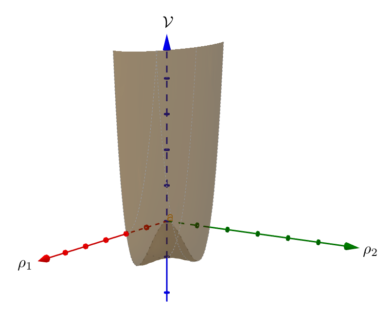
Figure 1: Profile of the potential in phase I

III.4 Phase II

The next situation corresponds to the existence of two minima, when,

$$\gamma\geq\lambda_{1}\frac{\mu_{2}^{2}}{\mu_{1}^{2}}\,,\hskip 28.45274pt\gamma\geq\lambda_{2}\frac{\mu_{1}^{2}}{\mu_{2}^{2}}\,,$$ (62)

excluding the half-plane of the phase I. This is the region over the planes $\gamma=\lambda_{1}\frac{\mu_{2}^{2}}{\mu_{1}^{2}}$ and $\gamma=\lambda_{2}\frac{\mu_{1}^{2}}{\mu_{2}^{2}}$, over the cone $\gamma^{2}=\lambda_{1}\lambda_{2}$. The phase I splits the region into two pieces where there exist two vacua, a false and the true vacuum (deepest).

The left side region in Fig. (1) denoted as II, has the dominant vacuum,

$$\rho_{1}=\sqrt{\frac{2\mu_{1}}{\lambda_{1}}}\,,\hskip 28.45274pt\rho_{2}=0\,,$$ (63)

with potential density,

$$V_{\textrm{II}}=-\frac{\mu_{1}^{4}}{\lambda}\,.$$

Also, this phase presents a false vacuum placed at,

$$\rho_{1}=0\,,\hskip 28.45274pt\rho_{2}=\sqrt{\frac{2\mu_{2}^{2}}{\lambda_{2}}}\,,$$ (64)

with potential energy density,

$$V^{\prime}_{\textrm{II}}=\frac{\mu_{2}^{4}}{\lambda_{2}}\,.$$

In the middle there is a saddle point placed at points in (51) and (52), with potential energy density,

$$V=-\frac{\lambda_{1}\mu_{2}^{4}-2\gamma\mu_{1}^{2}\mu_{2}^{2}+\lambda_{2}\mu_{1}^{4}}{\lambda_{1}\lambda_{2}-\gamma^{2}}\,.$$ (65)

See Fig. 2 to check the characterization of the minima structure in this phase.

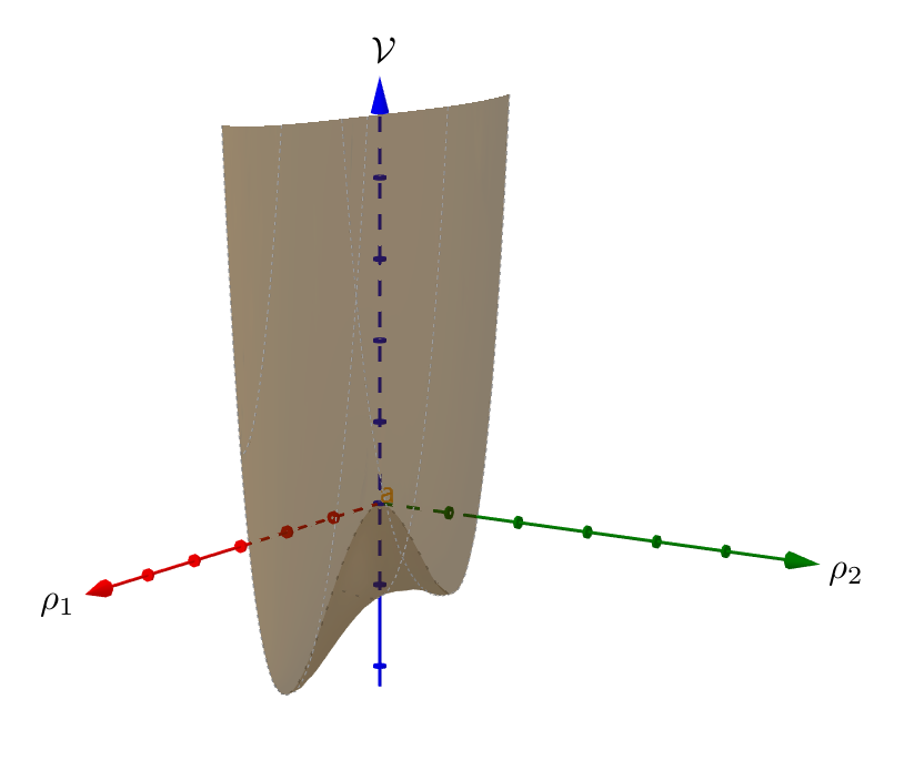
Figure 2: Profile of the potential in phase II

The right piece, denoted by II’ in Fig. (1) is similar to the situation just above but swapping indices $1$ and $2$, i.e., it is characterized by a dominant vacuum given by (64), and a false vacuum given by (63).

III.5 Phases III and IV

Now we analyze the situation where there occurs a unique vacuum. This happens in two situations.

The first situation, phases III and III’ in Fig.1, correspond to the vacuum located at (phase III),

$$\rho_{1}=0\,,\hskip 28.45274pt\rho_{2}=\sqrt{\frac{2\mu_{2}^{2}}{\lambda_{2}}}\,,$$

when

$$\lambda_{2}\frac{\mu_{1}^{2}}{\mu_{1}^{2}}<\gamma<\lambda_{1}\frac{\mu_{2}^{2}}{\mu_{1}^{2}}$$

or (phase III’),

$$\rho_{1}=\sqrt{\frac{2\mu_{2}^{1}}{\lambda_{1}}}\,,\hskip 28.45274pt\rho_{2}=0\,,$$

when,

$$\lambda_{1}\frac{\mu_{2}^{2}}{\mu_{1}^{2}}<\gamma<\lambda_{2}\frac{\mu_{1}^{2}}{\mu_{1}^{2}}$$

respectively, with minimal potential energies given in previous subsection. See Fig.3 for the potential profile of this phase.

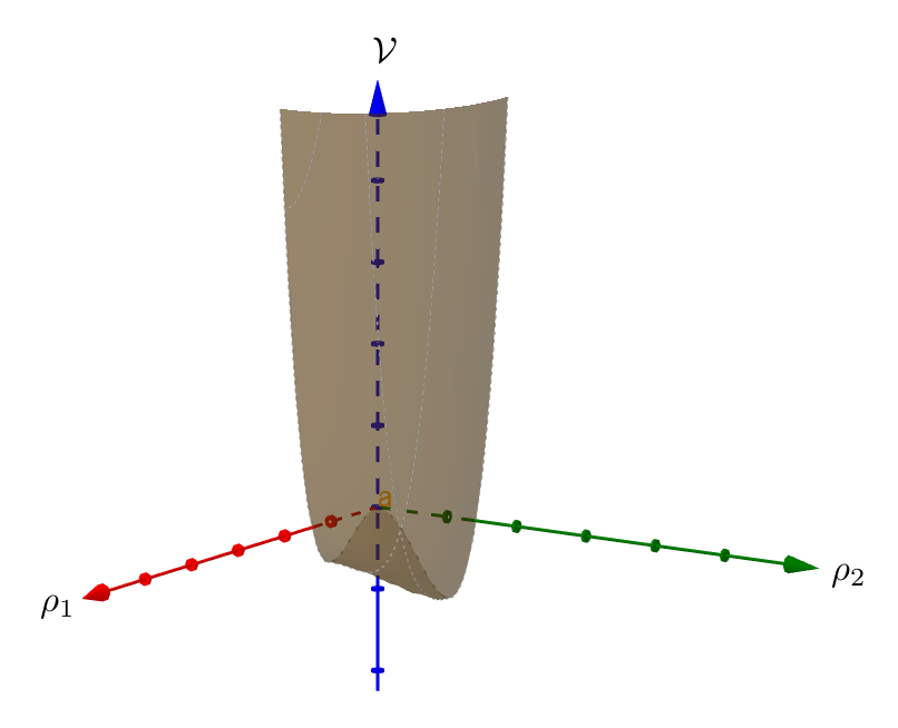
Figure 3: Profile of the potential in phase III

The second situation, phase IV in Fig. 1 happens when,

$$\gamma\leq\lambda_{1}\frac{\mu_{2}^{2}}{\mu_{1}^{2}}\,,\hskip 28.45274pt\gamma\leq\lambda_{2}\frac{\mu_{1}^{2}}{\mu_{2}^{2}}\,,$$

with the unique minimum placed at position given in (51) and (52) and with potential depth given in (65), see Fig. LABEL:potential4.

III.6 Phase V

Finally we obtain an degenerate vacuum when,

$$\gamma=\sqrt{\lambda_{1}\lambda_{2}}\,,\hskip 28.45274pt\frac{\lambda_{1}}{\lambda_{2}}=\frac{\mu_{1}^{4}}{\mu_{2}^{4}}\,,$$

which is a straight line corresponding to a generatrix of the cone $\gamma^{2}=\lambda_{1}\lambda_{2}$. The vacuum is degenerate along the elliptic curve (56) and its depth potential is,

$$V=-\frac{\mu_{1}^{2}\mu_{2}^{2}}{\sqrt{\lambda_{1}\lambda_{2}}}\,,$$

see Fig. LABEL:potential5.

IV Sign changes in $\mu^{2}$ parameters

In this section we complete the previous analysis for the cases where parameters $\mu_{1}^{2}$ and/or $\mu_{2}^{2}$ change sign.

IV.1 Case $\mu_{1}^{2}<0$ and $\mu_{2}^{2}>0$

Firstly, in this case the symmetric solution $\rho_{1}=\rho_{2}=0$ is a saddle point as it can be seen directly from (45).

The solutions of the kind $\rho_{1}=0$ and $\rho_{2}\not=0$, namely,

$$\rho_{2}^{2}=\frac{2\mu_{2}^{2}}{\lambda_{2}}\,,$$

can be realized as minima if,

$$\gamma>\lambda_{2}\frac{\mu_{1}^{2}}{\mu_{2}^{2}}\,,$$ (66)

as it can be seen from the expression of the hessian (45). Obviously solutions of the form $\rho_{2}=0$ and $\rho_{1}\not=0$ can not be realized.

Now let us analyze the case $\rho_{1}\not=0$ and $\rho_{2}\not=0$. In order to have non vanishing solutions we impose that expressions (51) and (52) to be positive, so that we arrive to the inequalities inside the cone,

$$\gamma<\lambda_{2}\,\frac{\mu_{1}^{2}}{\mu_{2}^{2}}\,,\hskip 28.45274pt\gamma>\lambda_{1}\,\frac{\mu_{2}^{2}}{\mu_{1}^{2}}\,,\hskip 28.45274pt-\sqrt{\lambda_{1}\lambda_{2}}<\gamma<\sqrt{\lambda_{1}\lambda_{2}}\,,$$ (67)

and this is a non empty region of parameters, and furthermore, for the solutions belonging to this set of inequalities we have a positive definite Hessian as it can be seen from (53). So in this region, the vacuum expectation values are given by (51) and (52), Also we must look outside the cone $\gamma>\sqrt{\lambda_{1}\lambda_{2}}$, and we find the inequalities,

$$\gamma>\lambda_{2}\,\frac{\mu_{1}^{2}}{\mu_{2}^{2}}\,,\hskip 28.45274pt\gamma<\lambda_{1}\,\frac{\mu_{2}^{2}}{\mu_{1}^{2}}\,,\hskip 28.45274pt\gamma>\sqrt{\lambda_{1}\lambda_{2}}\,,$$ (68)

Clearly this set of inequalities are incompatible, and there is no solution of this kind outside the cone.

Hence the phase space is simple in this case: we have a phase of type IV inside the cone and below the plane $\gamma=\lambda_{2}\frac{\mu_{1}^{2}}{\mu_{2}^{2}}$.

IV.2 Case $\mu_{1}^{2}>0$ and $\mu_{2}^{2}<0$

This case is entirely similar to the case above but swapping indices $1$ and $2$. the phase space is drawn in Fig. LABEL:rightI. Note that the phase IV has changed its location and phase III appears instead of phase III’.

IV.3 Case $\mu_{1}^{2},\mu_{2}^{2}<0$

It is easy to see that in this case, if we assume that $\gamma^{2}<\lambda_{1}\lambda_{2}$, the region for $\rho_{1}^{2}$ and $\rho_{2}^{2}$ being positive in (51) and (52) is that above both planes $\gamma=\lambda_{2}\frac{\mu_{1}^{2}}{\mu_{2}^{2}}$ and $\gamma=\lambda_{1}\frac{\mu_{2}^{2}}{\mu_{1}^{2}}$, and hence there is no way to have the phase $I$ outside the cone. Furthermore, by setting any of the $\rho$’s to zero, the other can not reach a minimum. Hence the only possibility for the minimum is,

$$\rho_{1}=0\,,\hskip 85.35826pt\rho_{2}=0\,,$$ (69)

which corresponds to the maximal symmetric vacuum. Similar situation occurs outside the cone, and only symmetric solution is possible.

V Instantons and Higgs Portal

In this section we generalize the results given in III and IV for the Higgs portal (38). More specifically in phase I we have two minima separated by a potential barrier while in phases II and II’ there are two asymmetric minima, one of them is a false vacuum.

These two cases are of interest by the following reasons:

• Potential I is the classical Mexican hat potential for which spontaneous symmetry breaking is restored by instantons effects.

• The potential II and II’ is metastable and decays to a true vacuum. However, when it decays to true vacuum, it transfers information about the physical parameters to true vacuum.

Interestingly the two cases mentioned above can be analyzed in the infrared limit assuming the boundary condition

$$\lim_{|x|\to\infty}\varphi_{1,2}(x)\to\pm v_{1,2}.$$ (70)

The equation of motion are

$${\ddot{\varphi}_{1}} = -\mu_{1}^{2}\varphi_{1}+{\bar{\lambda}}_{1}|\varphi_{1}|^{2}\varphi_{1}+{\bar{\gamma}}|\varphi_{2}|^{2}\varphi_{1},$$ (71)

$${\ddot{\varphi}_{2}} = -\mu_{2}^{2}\varphi_{2}+{\bar{\lambda}}_{2}|\varphi_{2}|^{2}\varphi_{2}+{\bar{\gamma}}|\varphi_{1}|^{2}\varphi_{2},$$ (72)

where

$${\bar{\lambda}}_{1,2}=\frac{\lambda_{1,2}}{\ell^{2}},~{}~{}~{}~{}~{}~{}~{}~{}~{}{\bar{\gamma}}=\frac{\gamma}{\ell^{2}}.$$ (73)

Although we cannot solve these equations analytically, we can try to find asymptotic solutions using the fact that both $\varphi_{1}$ and $\varphi_{2}$ tend to $v_{1}$ and $v_{2}$. Using the condition (70) and the fact that

$$v_{1}^{2} = \frac{-{\bar{\lambda}}_{2}\mu^{2}_{1}+{\bar{\gamma}}\mu_{2}^{2}}{{\bar{\gamma}}^{2}-{\bar{\lambda}}_{1}{\bar{\lambda}}_{2}}\,,$$ (74)

$$v_{2}^{2} = \frac{-{\bar{\lambda}}_{1}\mu^{2}_{2}+{\bar{\gamma}}\mu_{1}^{2}}{{\bar{\gamma}}^{2}-{\bar{\lambda}}_{1}{\bar{\lambda}}_{2}}\,,$$ (75)

The first and second equations become

$${\ddot{\varphi}_{1}} = -\left(\mu_{1}^{2}-{\bar{\gamma}}v_{2}^{2}\right)\varphi_{1}+{\bar{\lambda}}_{1}|\varphi_{1}|^{2}\varphi_{1},$$

$${\ddot{\varphi}_{2}} = -\left(\mu_{2}^{2}-{\bar{\gamma}}v_{1}^{2}\right)\varphi_{2}+{\bar{\lambda}}_{2}|\varphi_{2}|^{2}\varphi_{2}.$$ (76)

or in terms of the effective parameters

$${{\tilde{\mu}}_{1}}^{2} = \left(\mu_{1}^{2}-{\bar{\gamma}}v_{2}^{2}\right)=\frac{{\bar{\lambda}}_{1}({\bar{\gamma}}\mu_{2}^{2}-{\bar{\lambda}}_{2}\mu_{1}^{2})}{{\bar{\gamma}}^{2}-{\bar{\lambda}}_{1}{\bar{\lambda}}_{2}}$$

$${\tilde{\mu}}_{2}^{2} = \left(\mu_{1}^{2}-{\bar{\gamma}}v_{2}^{2}\right)=\frac{{\bar{\lambda}}_{2}({\bar{\gamma}}\mu_{1}^{2}-{\bar{\lambda}}_{1}\mu_{2}^{2})}{{\bar{\gamma}}^{2}-{\bar{\lambda}}_{1}{\bar{\lambda}}_{2}}.$$ (77)

Then the asymptotic solutions are

$${\bar{\varphi}}_{1}(t) = \pm\sqrt{\frac{{\tilde{\mu}}_{1}^{2}}{{\bar{\lambda}}_{1}}}\tanh\left[\sqrt{\frac{{\tilde{\mu}}_{1}^{2}}{2}}(t-t_{0})\right],$$ (78)

$${\bar{\varphi}}_{2}(t) = \pm\sqrt{\frac{{\tilde{\mu}}_{2}^{2}}{{\bar{\lambda}}_{2}}}\tanh\left[\sqrt{\frac{{\tilde{\mu}}_{1}^{2}}{2}}(t-t_{0})\right],$$ (79)

which are two uncoupled (dilute) instantons with effective parameters $({\tilde{\mu}}_{1},{\bar{\lambda}}_{1})$ and $({\tilde{\mu}}_{2},{\bar{\lambda}}_{2})$ respectively.

The stability of the vacua in the Higgs portal must satisfy

$${\tilde{\mu}^{2}}_{1}>0,~{}~{}~{}~{}~{}~{}{\tilde{\mu}^{2}}_{2}>0.$$ (80)

If ${\tilde{\mu}^{2}}_{1}={\tilde{\mu}^{2}}_{2}>0$, then the spontaneous symmetry breaking is restored by tunneling of instantons and if ${\tilde{\mu}^{2}}_{1}\neq{\tilde{\mu}^{2}}_{2}>0$, the state of higher energy becomes unstable through barrier penetration and this is an example of a false vacuum coleman1 .

As discussed in the previous sections, the physical implications that follow from our analysis are a consequence of the infrared approximation studied here and valid when (19) is fulfilled.

VI Conclusions

The spontaneous symmetry breaking phenomenon is the cornerstone of the standard model, chiral symmetry breaking and so on. However, the connection between tunneling and the relationship of Yang-Mills theory is not fully understood and, for this reason in this paper we have introduced a reinterpretation of the ultralocal Klauder limit that we call the infrared approximation in order to have a more physical view of the phenomenon.

In this work we have studied the case in which the depth of the well is $\ell\sim\mu^{-1}$ in such a way that the excitations are either confined or undergo tunneling between one vacuum to another.

Tunneling by instantons is a phenomenon that appears only in $2D$ but from the point of view of the infrared approximation studied in this paper, instanton tunneling emerges naturally (see eq. (18)). The relationship between these “infrared instantons” and Yang-Mills theory also appears quite naturally as shown in section II and follows from the gauge potential ansatz, namely $A^{a}_{\mu}=A^{a}_{\mu}(x^{2})$, is $O(4)$ invariant producing the well-known dimensional reduction as in a central field in classical mechanics.

Finally, a Higgs portal is considered as a way to understand the effect of scalar fields extras and the role that these can have in the case of cold dark matter. A discussion of this will be given elsewhere.

References

• (1) G. Bertone and D. Hooper, Rev. Mod. Phys. 90 (2018) no.4, 045002.
• (2) D. Carney, G. Krnjaic, D. C. Moore, C. A. Regal, G. Afek, S. Bhave, B. Brubaker, T. Corbitt, J. Cripe, N. Crisosto, A. Geraci, S. Ghosh, J. G. E. Harris, A. Hook, E. W. Kolb, J. Kunjummen, R. F. Lang, T. Li, T. Lin, Z. Liu, J. Lykken, L. Magrini, J. Manley, N. Matsumoto, A. Monte, F. Monteiro, T. Purdy, C. J. Riedel, R. Singh, S. Singh, K. Sinha, J. M. Taylor, J. Qin, D. J. Wilson and Y. Zhao, [arXiv:2008.06074 [physics.ins-det]].
• (3) I. de Martino, S. S. Chakrabarty, V. Cesare, A. Gallo, L. Ostorero and A. Diaferio, Universe 6 (2020) no.8, 107 doi:10.3390/universe6080107 [arXiv:2007.15539 [astro-ph.CO]].
• (4) E. Ferreira, G.M., [arXiv:2005.03254 [astro-ph.CO]].
• (5) C. Miller, A. L. Erickcek and R. Murgia, Phys. Rev. D 100 (2019) no.12, 123520
• (6) G. Bertone, D. Hooper and J. Silk, Phys. Rept. 405 (2005), 279-390
• (7) R. Engel et al. [FUNK Experiment], [arXiv:1711.02961 [hep-ex]].
• (8) P. A. Zyla et al. [Particle Data Group], PTEP 2020 (2020) no.8, 083C01
• (9) B. Patt and F. Wilczek, [arXiv:hep-ph/0605188 [hep-ph]].
• (10) G. Ballesteros, J. Redondo, A. Ringwald and C. Tamarit, JCAP 08 (2017), 001
• (11) A. Falkowski, C. Gross and O. Lebedev, JHEP 05 (2015), 057.
• (12) A. Eichhorn and M. Pauly, [arXiv:2005.03661 [hep-ph]].
• (13) M. Chianese, B. Fu and S. F. King, JCAP 06 (2020), 019. .
• (14) C. Englert, J. Jaeckel, M. Spannowsky and P. Stylianou, Phys. Lett. B 806 (2020), 135526
• (15) G. Arcadi, A. Djouadi and M. Raidal, Phys. Rept. 842 (2020), 1-180.
• (16) A. Filimonova and S. Westhoff, JHEP 02 (2019), 140
• (17) A. A. Belavin, A. M. Polyakov, A. S. Schwartz and Y. S. Tyupkin, Phys. Lett. B 59 (1975), 85-87.
• (18) G. ’t Hooft, Phys. Rev. D 14, 3432 (1976) Erratum: [Phys. Rev. D 18, 2199 (1978)].
• (19) G. ’t Hooft, Phys. Rept. 142 (1986), 357-387
• (20) F. R. Klinkhamer and N. S. Manton, Phys. Rev. D 30 (1984), 2212.
• (21) F. A. Schaposnik, Phys. Rev. D 18 (1978), 1183-1191.
• (22) C. G. Callan, Jr., R. F. Dashen and D. J. Gross, Phys. Lett. B 63 (1976), 334-340
• (23) R. Jackiw and C. Rebbi, Phys. Rev. Lett. 37 (1976), 172-175.
• (24) R. Jackiw and C. Rebbi, Phys. Rev. D 13 (1976), 3398-3409.
• (25) For a review on classical Yang-Mills solutions see for example, A. Actor, Rev. Mod. Phys. 51 (1979), 461
• (26) A. M. Polyakov, Nucl. Phys. B 120 (1977), 429-458.
• (27) S. R. Coleman, Phys. Rev. D 15 (1977), 2929-2936.
• (28) C. G. Callan, Jr. and S. R. Coleman, Phys. Rev. D 16 (1977), 1762-1768.
• (29) S. R. Coleman, Subnucl. Ser.  15, 805 (1979).
• (30) M. Mariño, “Instantons and Large N: An Introduction to Non-Perturbative Methods in Quantum Field Theory,” (unpublished).
• (31) M.  B.  Paranjape, “The Theory and Applications of Instanton Calculations", Cambridge University Press (2017).
• (32) E. Fradkin, Lectures Notes on Quantum Field Theory, Chap 9, UIUC (unpublished).
• (33) J. R. Klauder, Commun. Math. Phys. 18 (1970), 307-318
• (34) M. Pilati, Phys. Rev. D 28, 729 (1983).
• (35) M. Henneaux, M. Pilati and C. Teitelboim, Phys. Lett.  110B, 123 (1982).
• (36) C. Teitelboim, Phys. Rev. D 25, 3159 (1982).
• (37) J. Gamboa, Phys. Rev. Lett.  74, 1900 (1995).
• (38) J. Gamboa and F. Mendez, Nucl. Phys. B 600, 378 (2001).
• (39) J. Gamboa, Phys. Rev. D 53, 6991 (1996).
• (40) C. J. Isham, IMPERIAL/TP/88-89/30.
• (41) E. Anderson, Gen. Rel. Grav. 36 (2004), 255-276.
• (42) A. V. Belitsky, S. Vandoren and P. van Nieuwenhuizen, Class. Quant. Grav. 17 (2000), 3521-3570
• (43) D. Diakonov, Prog. Part. Nucl. Phys. 51 (2003), 173-222