Gubkina str. 8, 119991, Moscow, Russia
bPeoples Friendship University of Russia,
Miklukho-Maklaya str. 6, 117198, Moscow, Russia
Holographic Anisotropic Model for Light Quarks with Confinement-Deconfinement Phase Transition
Abstract
We present a five-dimensional anisotropic holographic model for light quarks supported by Einstein-dilaton-two-Maxwell action. This model generalizing isotropic holographic model with light quarks is characterized by a Van der Waals-like phase transition between small and large black holes. We compare the location of the phase transition for Wilson loops with the positions of the phase transition related to the background instability and describe the QCD phase diagram in the thermodynamic plane – temperature and chemical potential . The Cornell potential behavior in this anisotropic model is also studied. The asymptotics of the Cornell potential at large distances strongly depend on the parameter of anisotropy and orientation. There is also a nontrivial dependence of the Cornell potential on the boundary conditions of the dilaton field and parameter of anisotropy. With the help of the boundary conditions for the dilaton field one fits the results of the lattice calculations for the string tension as a function of temperature in isotropic case and then generalize to the anisotropic one.
Keywords:
AdS/QCD, holography, phase transition, Wilson loops, light quarks1 Introduction
Experimental research of the phase transitions structure for the quark matter is one of important problems of modern collider facilities 1710.09425 . The phase diagram in the thermodynamical plane – temperature and chemical potential – has been only studied experimentally for small and large values (RHIC, LHC) on the one hand and for finite and small values (SPS) on the other. The study of the phase diagram in between these two selected cases is one of the main goals of FAIR and NICA projects.
According to results of heavy ion collision (HIC) experiments at RHIC and LHC the quark gluon-plasma (QGP) should exist at large temperatures and densities. Temperature of the confinement/deconfinement phase transition most likely depends on chemical potential, i.e. the phase transition can be displayed on the -plane. Under some circumstances QGP behaves like an almost viscous liquid with an initial spatial anisotropy Strickland:2013uga , therefore phase transition in anisotropic QCD should be considered.
Perturbative methods are not suited for the QGP studies. Several calculations have been performed within the lattice approach Philipsen:2010 ; Boyda:2017dyo ; Philipsen:2019rjq ; Ratti , but lattice calculations cannot provide full phase transition picture in -plane because of so-called sign problems. It is holographic duality Solana ; IA ; DeWolf that opens up an alternative approach to the QCD phase transitions’ researches. Among other things, this approach has a natural framework to deal with spatial anisotropy Mateos:2011ix ; Mateos:2011tv ; Rebhan:2011vd ; Giataganas:2012 ; Cheng:2014sxa ; Cheng:2014qia ; Jain:2014vka ; AG ; AGG ; Giataganas:2017koz ; ARS-2019qfthep . Note that anisotropic lattice calculations have been performed in Forcrand2018 .
Holographical QCD (HQCD) as a phenomenological model has to describe QCD at all energy scales. That means to reproduce the usual QCD results obtained by perturbative theory at short distances and Lattice QCD results at large distances (confinement etc.). The other purpose of HQCD concerns intermediate energy scales. It has to give theoretical results, that are in agreement with experiments, as well as to predict new results especially in extremal conditions such as hight density or large chemical potential.
HQCD is formulated as 5-dimensional theory, where the 5-dim background usually is a deformed version of a 5-dimensional Schwarzschild-AdS or Reissner-Nordström Schwarzschild-AdS space time. A scalar (dilaton) field’s dynamics describes the running coupling in 4-dim quantum theory, and the 5-th coordinate playes a role of an energy scale.
Different isotropic holographic QCD models are distinguished by the choice of the warp factor Kiritsis ; 1301.0385 ; yang2015 ; Yang-2017 ; Dudal:2017max ; Dudal:2018ztm ; Mahapatra:2019uql ; Ebrahim:2020qif ; He:2020fdi ; Zhou:2020ssi . Models with different warp factors describe different phenomenological models. In the isotropic case there are special warp factors that describe the QCD for light or heavy quarks yang2015 ; Yang-2017 . It is interesting to consider a more complicated version of the warp factor that describes model for both light and heavy quarks. It happens that to describe chiral phase transition one has to modify holographic model essentially by introducing additional scalar fields Fang:2015ytf ; Ballon-Bayona:2020qpq .
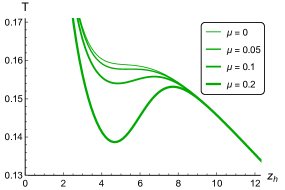
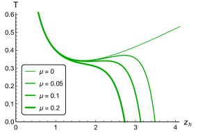
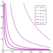
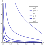
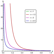
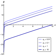
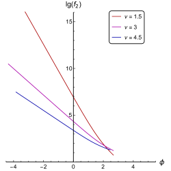
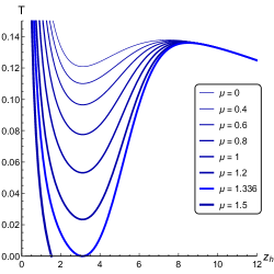
Qualitative look of the confinement/deconfinement phase transition on -plane for different quarks’ mass in isotropic media is displayed in Fig.1. Phase transition of the light quarks is supposed to have a crossover for small chemical potentials and a first-order phase transition for large chemical potentials (Fig.1.A). This picture was obtained in Yang-2017 . Phase transition of the heavy quarks, on the opposite, has a first-order phase transition for small chemical potentials and a crossover for large chemical potentials (Fig.1.B). Difference in the behavior of holographic models for heavy and light quarks is caused by difference in dependences of temperature on the horizon size in these models (Fig.2). Here and below chemical potential and temperature are taken in GeV units and in GeV-1.
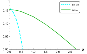
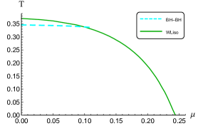
A B
There are several reasons to consider anisotropic versions of the holographic models mentioned above: to reproduce the experimental data for the energy dependence of the total multiplicity AG , to describe inverse magnetic catalysis Bohra:2019ebj ; Gursoy:2018ydr ; Gursoy:2020 ; He:2020fdi ; Ballon-Bayona:2020xtf or to take into account anisotropic geometry of colliding ions.
In AR-2018 the anisotropic holographic model for heavy quarks was studied. A peculiar feature of the model is the relation between anisotropy of the background and anisotropy of the colliding heavy ions geometry. In AR-2018 anisotropy is described by a special parameter , and it’s value of about gives the dependence of the produced entropy on energy in accordance with the experimental data for the energy dependence of the total multiplicity of particles produced in heavy ion collisions Alice . Isotropic holographic models had not been able to recover the experimental multiplicity dependence on energy (AG and refs therein). As shown in ARS-2019plb , the solution AR-2018 describes smeared confinement/deconfinement phase transitions. This model also indicates the relations of the fluctuations of the multiplicity, i.e. the entanglement entropy, with the phase transitions APS .
The purpose of this paper is to perform similar investigation for the model describing the light quarks. As in case of the heavy quarks AR-2018 , the anisotropic model for light quarks considered in this work is described by the parameter again.
A B
We also study the Cornell potential behavior in this anisotropic model and discuss a nontrivial dependence of the Cornell potential on boundary conditions of the dilaton field and parameter of anisotropy. Particular forms of -function and their connection to the boundary condition for the scalar field are investigated. As a result we suggest a boundary definition that allows to fit string tension behavior from Lattice QCD Bali2001 .
Holographic calculations for heavy and light quarks models are essentially different since solutions for the heavy quarks model can be expressed explicitly, unlike the model of light quarks, where the solution is presented in quadratures. Therefore the generalization to anisotropic model of the light quarks is a more complicated task.
The paper is organized as follows. In Sect. 2.1 we present the action and the ansatz that solves the EOM for the anisotropic model with symmetry in transversal directions. In Sect. 2.2 we briefly describe the solutions of the considered model. The thermodynamics of the background is described in Sect. 3.1. In Sect. 3.2 we compare the position of the phase transition for Wilson loops with the positions of phase transitions related to the background instability in the thermodynamical plane – temperature and chemical potential . We end the paper with the discussion of future directions of research on the subject.
2 Model
2.1 Metric and EOM
We take the action in Einstein frame
| (1) | |||
| (2) |
where is the scalar field, and are the coupling functions associated with the Maxwell fields and correspondingly, is the constant and is the scalar field potential. Thus (1) is the same action that was used in AR-2018 .
To consider action (1) let us take the ansatz in the following view:
| (3) | |||
| (4) |
where is the AdS-radius, is the warp factor, is its half-power, is the blackening function and is the parameter of anisotropy. Following Yang-2017 we choose (4) for the warp factor to get the solution for the light quarks. Therefore the EOM simplifies to:
| (5) | |||
| (6) | |||
| (7) | |||
| (8) | |||
| (9) | |||
| (10) |
Excluding anisotropy and normalizing to the AdS-radius, i.e. putting , and into (5)–(10), one can get the expressions that fully coincide with the EOM (2.12)–(2.16) from Yang-2017 . We consider the general form of the boundary conditions:
| (11) | |||
| (12) | |||
| (13) |
where is a size of horizon and is the boundary condition point located between 0 and . The case of corresponds to Yang-2017 and corresponds to AR-2018 . The choice of the boundary condition for the scalar field discussed in details in Sect.2.2.3.
In this paper we assume , , to make our solution agree with results from Yang-2017 in the isotropic case. These values are due to the mass spectrum of meson with its excitations and to the lattice results for the phase transition temperature. We use the same values of , and for anisotropic case, as we still do not have anisotropic lattice data for the spectrum.
2.2 Solution
To solve EOM (5)–(10) we need to determine the form of the coupling function . Choosing it we base on our previous experience in anisotropic heavy quarks model AR-2018 and also follow the proposition for the isotropic light quarks model Yang-2017 , that reproduces the Regge spectrum:
| (14) |
i.e. is the same as for “heavy quark model” in AR-2018 .
Solving (6) with coupling function (14) and boundary conditions (11) gives the same answer as in AR-2018 ; yang2015 ; Yang-2017 :
| (15) |
Note that to obtain given by (15) in this work we take the simplest form of the coupling function . This choice isn’t the only possible one (see for example Yang-2020 ), but comparison of advantages and disadvantages of different forms of is not the subject of the current discussion.
2.2.1 Blackening function
A B
C D
| (16) |
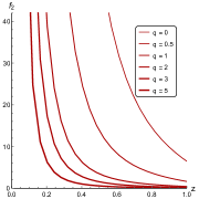
On Fig.3 we see behavior for different chemical potentials and anisotropy parameter values. For zero blackening function monotonously decreases (Fig.3.A), nonzero chemical potentials lead to the appearence of the second horizon that is decreasing with increasing . For small the second horizon doesn’t matter, but at some moment it becomes lesser than the fixed one and continues decreasing while increasing . From this moment it starts to play the main role and the fixed horizon loses actual influence. For larger we also have lesser second (moving) horizon values.
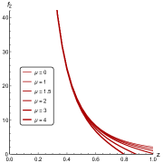
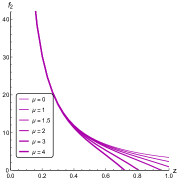
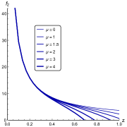
On Fig.4 blackening function curves for different and fixed chemical potential are displayed. For zero chemical potential (Fig.4.A) the blackening function decreases faster near the horizon for lesser , and this tendency continues for non-zero values in one form or another. The second (non-fixed) horizon is lesser for larger values (Fig.4.C,D).
Solution (2.31) from Yang-2017 satisfies our equation (7) for and and can be obtained from (16) putting .
A B
C D
A B C
A B C
A B C
2.2.2 Coupling function
Fig.7 shows coupling function behavior for different chemical potential and anisotropy parameter values. The coupling function tends to zero without chemical potential, and the larger and we have the faster decreases. This can also be seen from Fig.7. On the opposite, the larger charge makes to decrease more slowly for the fixed chemical potential value (Fig.7). In isotropic case (Fig.7).
Appropriate solutions require positive values. As we can see from plots of Fig.4-7, the considered region limited by the horizon with lesser fullfills this requirement.
Note, that the function is taken at hoc, while is found from EOM. The reason for this is the following. In spite of the fact that and are included into the action symmetrically, their roles are quite different. Coupling function provides the chemical potential and is related with the Regge spectrum, while specifies the anisotropy. We use the electric ansatz for the first Maxwell field and the magnetic one for the second like in AGG . Technically one can fix and find from EOM, but we do not have restrictions and requirements for the form of -function.
2.2.3 Scalar field
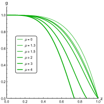
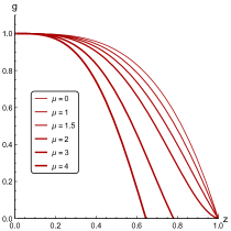
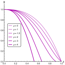
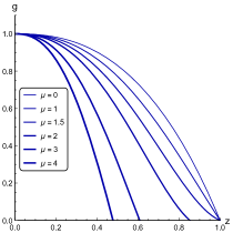
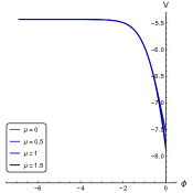
We should reproduce the correct behavior of the string tension on temperature. The condition (13) for can give the behavior considered in ARS-2019qfthep (for heavy quarks and, as it would be seen, for light quarks situation is the same). Solving (8) with boundary condition (13) gives
| (18) |
A B
C D
In the anisotropic case for the dilaton field has a logarithmic divergence . There are no divergences in the isotropic case for the dilaton field and the expression is reduced as:
| (19) |
Note that boundary conditions influence on the temperature dependence of string tension (i.e. on the coefficient in the linear term of Cornell potential). String tension should decrease while temperature increases and drop to zero after the confinement/deconfinement phase transition Digal:2005ht ; Cardoso:2011hh ; Bicudo:2010hg . To keep this behavior on the one hand and avoid divergences in anisotropic cases on the other hand we generalize boundary condition for dilaton field as He:2010ye , where can be a function of . Conditions AR-2018 or Yang-2017 are it’s particular cases.
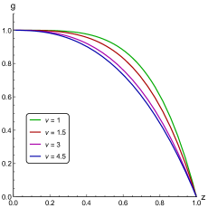
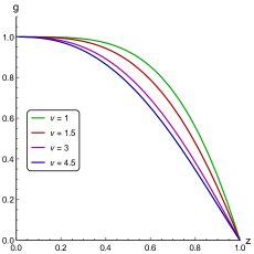
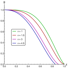
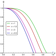
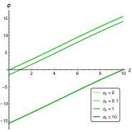
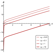
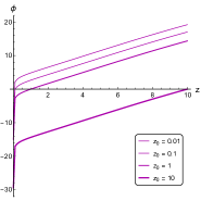
As we can see from Fig.8.A, even can be hardly distinguished from the in the isotropic case. This allows to assume that the results for sufficiently small reproduce the proper behavior of the scalar field. On the other hand the difference between various cases can be used to fit the experimental data in the future. The dilaton field’s dependence on is a monotonically increasing function (Fig.8). This function has finite negative value near in isotropic case and decreases quickly in anisotropic cases (Fig.8.B-D). We can also see that in this case the behavior depends on the anisotropy parameter rather weakly.
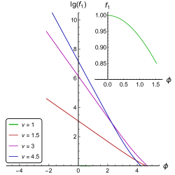
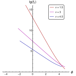
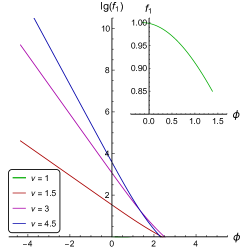
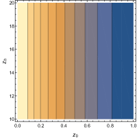
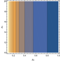
Since the function is monotonic, we reconstruct the form of and as functions of (Fig.9). Both functions decrease quickly and monotonically while increasing . The first (top) line of Fig.9 presents (Fig.9.A) and (Fig.9.B) for and different anisotropies in logarythmic scale (except for ). The second (bottom) line show the same plots for . The increasing of the boundary has rather weak effect on the shape of the coupling functions and mainly shifts them to the left, to lower -values.
A B
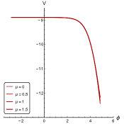
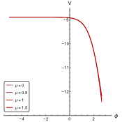
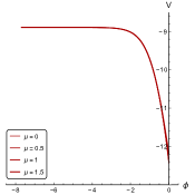
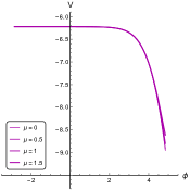
2.2.4 Scalar potential
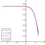
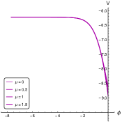
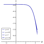
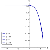
A B C
| (20) |
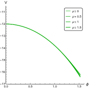
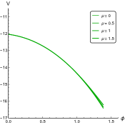
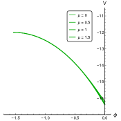
that transforms into (2.32) from Yang-2017 for . We can see that potential (20) does not depend on the boundary conditions or the dilaton field, as equation (10) inculdes the dilaton field’s derivative, not the dilaton itself. But behavoir does depend on them.
On Fig.10 -curves for different boundaries are presented. Scalar potential is plotted till the horizon, i.e. for . We can see that the increasing of the boundary doesn’t actually affect the shape of , just shifts the whole curve to the left, to lower -values. Chemical potential influence on the scalar field is visible, but weak near the horizon only and therefore can be neglected.
A B
C D
3 Confinement/deconfinement phase transition
3.1 Temperature and entropy
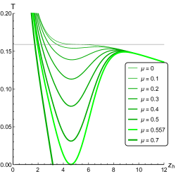
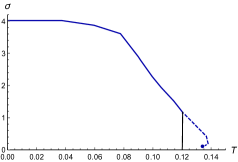
Fig.11.A shows that in isotropic case for temperature is a monotonically decreasing function of horizon. Increasing chemical potential makes -function three-valued at some interval, and local minimum appeares. As we will see below, this is directly related to the Hawking-page-like confinement/deconfinement phase transition. Indeed, in the isotropic case first-order phase transition for light quarks shouldn’t exist near zero chemical potential and we should see a crossover (Fig.21.B). The larger chemical potential is the lesser temperature value at this local minimum becomes. For local minimum temperature and second horizon appears.
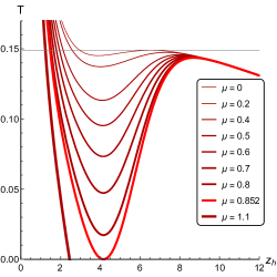
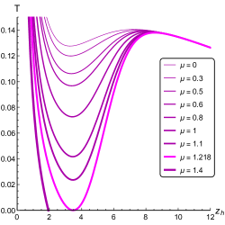
In the anisotropic case global behavior of temperature persists, but it is a three-valued function for already and the second horizon appears at about for (Fig.11.B), for (Fig.11.C). and for (Fig.11.D). This indicates that the Hawking-Page-like phase transition line should exist even in the absence of chemical potential, and Fig13.B confirms this.
A B
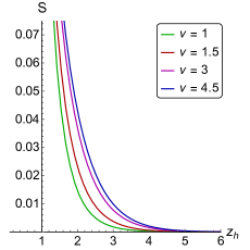
For metric (3) and the warp factor (4) entropy becomes
| (22) |
It decreases monotonocally and quickly with horizon growth (Fig.13.A).
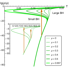
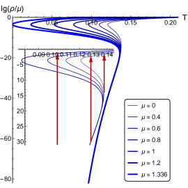
The BH-BH phase transition caused by three-valued temperature function produces a jump of density , that is a coefficient in expansion:
| (23) |
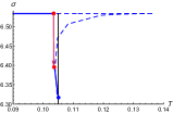
On Fig.12 ratio as a function of temperature for primary isotropic solution (, Fig.12.A) and anisotropic solution (, Fig.12.B) are plotted in logarithmic scale. Vertical red arrows show the BH-BH transition direction. Function is a three-valued function of as expected, and we can see that collapse from small black holes (larger ) to the large ones (smaller ) is accompanied by a sharp rise of the density for any appropriate chemical potential.
A B
To get Hawking-Page-like transition line (BH-BH phase transition) we need to consider free energy as a function of temperature:
| (24) |
While , i.e for small chemical potentials, we integrate to . When second horizon where appears, one should integrate to it’s value, i.e. to for , , to for , and to for , . These conditions determine the end-point of the phase diagram, i.e. maximum permissible chemical potential for chosen . Thus increasing anisotropy parameter allows larger chemical potentials, but reduces the temperature.
On Fig.13.B Hawking-Page-like phase transition for is depicted. In isotropic case BH-BH phase transition starts from a critical point , that fully coincides with previous result in Yang-2017 .
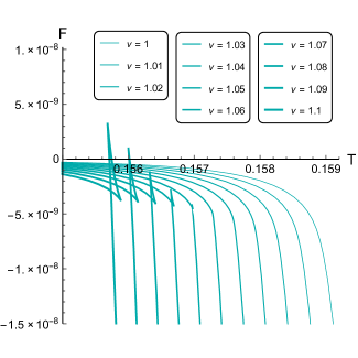
For the Hawking-Page-like phase transition the free energy should be a multi-valued function of temperature. Graphically it is displayed as a “swallow-tail”. The point where the free energy curve intersects itself determines the Hawking-Page-like phase transition temperature. On Fig.14 the free energy as a function of temperature for different values of in the absence of chemical potential is plotted. We see a smooth free energy curve for , therefore no self-intersection and no Hawking-Page-like phase transition for exists. For an obtuse angle appears on the curve – this is a germ of the “swallow-tail”. The larger becomes the more pronounced the “swallow-tail” is. So turning the anisotropy on causes the gap between and the starting point of the Hawking-Page-like line on the confinement/deconfinement phase diagram to close. Slight anisotropy with is enough to make this type of phase transition exist for all chemical potential values .
3.2 Temporal Wilson loops
Following ARS-2019plb we consider temporal Wilson loops in anisotropic background to calculate the parameters of Cornell potential and find the conditions of confinement/deconfinement phase transition. Calculations for the Wilson loops were done in the string frame. To determine the confinement/deconfinement condition and the string tension let us study the asymptotics of the Nambu-Goto action for the test string at large character length of the string . At one has
| (25) |
Like it was in ARS-2019plb , we take the world sheet parameterized as
Angle defines orientation of the Wilson loop in the considered background. The string tension
| (26) |
obviously depends on the dilation field boundary conditions. Point is the position of the dynamical wall, where . In isotropic case this result coinsides with Yang-2017 .

A


B C
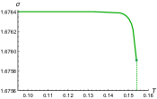
String tension dependence on the boundary point and horizon for isotropic case (Fig.15.A) and both orientations of anisotropic case (Fig.15.B,C) is presented. The behavior of is similar for and . Adding chemical potential doesn’t change the main picture as well. For fixed value larger leads to lesser . However, the string tension for fixed depends on weakly in all cases (Fig. 18). Due to the boundary condition the string tension slowly decreased with temperature till the very end, where it drops sharply to zero. This behavior persists for any , and values.
A B
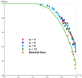
The string tension behavior in Lattice QCD was discussed in Laermann:2003cv ; Digal:2005ht ; Cardoso:2011hh ; Bicudo:2010hg ; J.P.:2020xmq . It was shown that is a decreasing function, but different factors can influence the particular form of the curve. Therefore fitting the experimental data could help to specify the model’s parameters. In particular, it is interesting to consider the boundary as a function and use it to fit the lattice results.
To get the best matching of isotropic with the lattice calculations Cardoso:2011hh ; Bicudo:2010hg we use the function
| (27) |
In this case the string tension decreases significantly faster than for (Fig.16). For anisotropic cases, where we do not have lattice data, we use the same function (27) and get the temperature dependences presented in Fig.17.A and B.
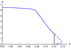
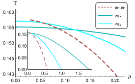
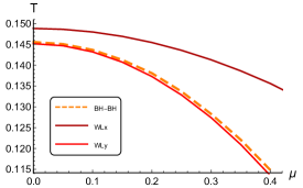
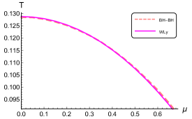
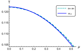
On Fig.17–19 string tension as function of temperature for different boundary limits and different chemical potential values are presented. Dotted lines on A-plots indicate the WL phase transition, when the connected string configuration changes to the disconnected one and the string tension drops to zero. Black solid lines on B (longitudinal orientation) and C (transversal orientation) plots show the BH-BH phase transition, when the connected string configuration in the first thermodynamic phase changes to disconnected string configuration in the second thermodynamic phase; dashed blue lines depict the string tension values for the temperatures higher than the temperature of the BH-BH phase transition. In anisotropic cases (B, C) string tension can be multi-valued function for some values of temperature.
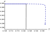
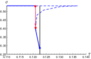
A B C
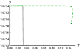
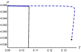
A B C
In all plots of Fig.18 and Fig.19 can be multi-valued function due to the multi-valued function of temperature on the size of horizon . To understand the behavior of the string tension on temperature we should use the knowledge about the BH-BH phase transitions structure.
In the considered case we have two thermodynamic phases – small black holes and large black holes – and a phase transition between them. The end point of in all plots is indicated by blue or green dot. After this point dynamical wall (DW) for the effective potential does not exist anymore and the connected string configuration disappears, that indicates the WL phase transition.
On Fig.18, 19 solid black (vertical) lines show the BH-BH phase transition for the chosen set of parameters and orientation. For isotropic case (Fig.19.A) and longitudinal orientation of anisotropic case (Fig.18.B, Fig.19.B) multi-valued (dashed) branch lies rather far from the BH-BH transition and does not interfere with it. Transversal orientation has a specific feature: multi-valued branch intersects the BH-BH transition line and thus starts to play significant role in the general phase transition process. The string tension has a phase transition at lower temperatures than the temperature of the BH-BH phase transition. At this temperature the connected string configuration with first string tension value in first thermodynamic phase is changed by the connected string configuration with second string tension value in second thermodynamic phase, . Red arrows on Fig.18.C and 19.C show these jumps of the string tension. We also see that non-zero chemical potential suppresses this effect, making the interval where the lowest part of the multi-valued -branch is realized, narrower (compare Fig.18.C for and Fig.19.C for ).
To get full picture we need to consider lines corresponding to Wilson loops and depending on quarks pair orientation. As the current model differs from the previous one by the form of the warp factor only, all the reasoning in AR-2018 ; ARS-2019plb remains applicable here. Therefore the dynamical wall equations become:
| (28) | |||
| (29) |
for longitudinal () and transversal () direction correspondingly.
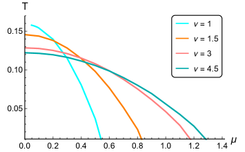
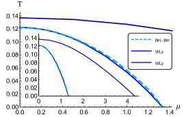
The resulting phase transition lines, determined by the Wilson loops (along with the Hawking-Page-like phase transition lines) for the isotropic and anisotropic cases are showed on Fig. 20.
A B
C D
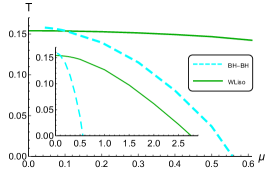
On Fig. 20.A the isotropic case is depicted. The confinement/deconfinement phase transition is mostly determined by the Hawking-Page-like transition (BH-BH transition). Wilson loop is sufficient in a small region of crossover for , i.e. till the point , where two phase transition lines intersect.
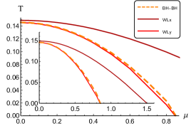
In the anisotropic case the isotropic Wilson line evolves into the line corresponding to longitudinal Wilson loop. Starting from the longutudinal Wilson line lies above the Hawking-Page-like and doesn’t actually influence the phase transition. For larger anisotropy longitudinal Wilson line has lower temperature values, but the difference between it and the Hawking-Page-like line increases with (Fig. 20.A-D). Phase transition line corresponding to the transversal Wilson loop almost coincides with the Hawking-Page-like line scaled, so there is no evident crossover region as it was in anisotropic case. Therefore influence of the transversal Wilson line and the Hawking-Page-like line on the confinement-deconfinement phase transition could be hardly distinguished from each other.
4 Conclusion
We have considered the anisotropic holographic model for light quarks. This model is invariant in the transversal directions with the unique anisotropy scaling factor supported by the Einstein-Dilaton-two-Maxwell action. The analogous model for heavy quarks was presented in AR-2018 . We have found characteristic features inherent in the description of light quarks within the holographic approach. Thermodynamical peculiar properties and their influence on the confinement/deconfinement phase diagram are considered.
A B
A B
C D
Unlike the heavy quarks model (Fig.21.B) AR-2018 , the Hawking-Page-like phase transition line does not break at a relatively high temperature, but lasts till (Fig.21.A). Also longitudinal orientation of quarks pairs does not contribute to confinement/deconfinement phase transition, so the influence is shared by the Hawking-Page-like and the transversal Wilson loop. Transfer of the main role in the phase transition looks rather smooth and simple and is not accompanied by jumps as it was in heavy quarks model AR-2018 .
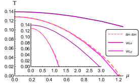
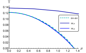
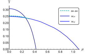
Plots on Fig.22 show the features of the phase diagram in more details. For (Fig. 22.C) and (Fig. 22.D) the Hawking-Page-like phase transition dominates for small chemical potentials (till and correspondingly), then the transversal Wilson loop takes over control providing narrow strip of the crossover for larger chemical potentials. However these effects seem to be rather weak, so practically the crossover region is unlikely to be registered for the light quarks confinement/deconfinement phase transition. For the transversal Wilson line lies right under the Hawking-Page-like line, so, strictly speaking, it is the transversal component that determines the confinement-deconfinement phase transition (Fig. 22.B). On the other hand the Hawking-Page-like line is located too close to make the crossover tangible.
Let us note that some interesting features appear for light quarks model for small anisotropy already. For example weak anisotropy with was considered (Fig. 22.A). Generally the phase transition picture for such a slight anisotropy is the same as in the isotropic case. When the anisostropy is turned on the crossover region narrows. For it end at the point . Actually the length of the crossover seems to be the most essential manifestation of anisotropy. It’s width shouldn’t be large as longitudinal and transversal Wilson lines are rather close to each other and for both of them lie above the Hawking-Page-like curve and do not affect the confinement/deconfinement phase transition.
Within the change of the boundary conditions of the dilaton field the form of the string tension dependence on temperature in isotropic case can be qualitatively fit by the lattice results (Fig.17.A). Keeping the same boundary condition for the anisotropic case we obtain realistic string tension behavior. In both models for heavy and light quarks can be a multi-valued function for high temperatures. The appearance of the multi-valued is the consequence the multi-valued temperature on the size of horizon for some set of parameters. The end point of is interpreted as a point of the phase transition associated with the Wilson loop (i. e. undergoes a jump to zero and the connected configuration is replaced by the disconnected one). Also undergoes a jump to zero due to the BH-BH phase transition, when the phase transition happens from first thermodynamic phase with connected string configuration to second thermodynamic phase with disconnected string configuration. As it was shown on Fig.18.C and Fig.19.C, the string tension has the phase transition – a jump of the string tension value to the string tension value , . This transition happens for lower temperatures than the BH-BH phase transition temperature and can be interpreted as the transition between quarkyonic and hadronic phases of QGP.
In both models (for heavy and light quarks) can be a multi-valued function for high temperatures. The appearance of multi-valued behavior is interpreted as a transition associated with the Wilson loop (i. e. undergoes a jump to zero and the connected configuration is replaced by the disconnected one). For weak anisotropization (), the BH-BH transition competes with the transition for the Wilson loop and for small chemical potentials () the transition for the Wilson loop is dominant. The result plots of the confinement/deconfinement phase transition on -plane for light and heavy quarks’ mass in anisotropic media are displayed in Fig. 21 and Fig. 22. We can see that the phase transitions structure is more complex in the anisotropic case than is isotropic one (Fig. 21 and Fig. 22 can be compared with Fig. 1).
Let us remind that the choice of the model AG , that is a starting point of our consideration of the anisotropic models, was motivated by agreement of the energy dependence of the produced entropy with the experimental data for the energy dependence of the total multiplicity of particles produced in HIC ALICE ; ATLAS . It would be interesting to study the change in the produced entropy under deformations of the anisotropic model AG with which we are dealing in this article. Also it would be interesting to study modification of the entanglement entropy, compare with Dudal:2018ztm ; APS .
This leads us to the next step for obtaining more realistic model – to investigate some kind of a mixed model, where both heavy and light quarks would be included. Study of such a mix should be rather instructive for better understanding of confinement/deconfinement phase transition and futher interpretations of experimental data. This model should also be fully anisotropic because of presence of external magnetic field. Analagous consideration inspired by Gursoy:2018ydr was already perfomed for heavy quarks only in 2011.07023 , see also Gursoy:2020 .
The holographic entanglement entropy (HEE) can be related to the phase transitions in quark matter, therefore it is interesting to calculate the HEE for the considered light quarks anisotropic model and compare the results with APS ; Arefeva:2019dvl ; Slepov:2019guc . Also drag forces and tensions for spatial Wilson loops can be compared following IADrag . Main considerations for heavy quarks can be found in 2012.05758 .
We hope that the results presented in this paper and their further possible adjustment to the phenomenological data can be of interest for experiments at the future facilities of FAIR, NICA, for RHIC’s BES II program and CERN, III run.
Acknowledgments
This work is supported by RFBR Grant 18-02-40069 and partially (I.A. and P.S.) by the “BASIS” Science Foundation grant No. 18-1-1-80-4.
References
- (1) A. Andronic, P. Braun-Munzinger, K. Redlich and J. Stachel, “Decoding the phase structure of QCD via particle production at high energy”, Nature 561, no. 7723, 321 (2018) [arXiv:1710.09425 [nucl-th]]
- (2) M. Strickland, “Thermalization and isotropization in heavy-ion collisions”, Pramana 84, 671 (2015)
- (3) O. Philipsen, “Lattice QCD at non-zero temperature and baryon density”, [arXiv:1009.4089 [hep-lat]]
- (4) D. Boyda, V. G. Bornyakov, V. Goy, A. Molochkov, A. Nakamura, A. Nikolaev and V. I. Zakharov, “Lattice QCD thermodynamics at finite chemical potential and its comparison with Experiments”, [arXiv:1704.03980 [hep-lat]]
- (5) O. Philipsen, “Constraining the QCD phase diagram at finite temperature and density”, [arXiv:1912.04827 [hep-lat]]
- (6) C. Ratti, “QCD at non-zero density and phenomenology”, PoS LATTICE2018 004 (2019)
- (7) J. Casalderrey-Solana, H. Liu, D. Mateos, K. Rajagopal and U. A. Wiedemann, “Gauge/String Duality, Hot QCD and Heavy Ion Collisions”, Cambridge University Press (2014) [arXiv:1101.0618 [hep-th]]
- (8) I. Ya. Aref’eva, “Holographic approach to quark-gluon plasma in heavy ion collisions”, Phys. Usp. 57, 527 (2014)
- (9) O. DeWolfe, S. S. Gubser, C. Rosen and D. Teaney, “Heavy ions and string theory”, Prog. Part. Nucl. Phys. 75, 86 (2014) [arXiv:1304.7794 [hep-th]]
- (10) D. Mateos and D. Trancanelli, “The anisotropic N=4 super Yang-Mills plasma and its instabilities,” Phys. Rev. Lett. 107, 101601 (2011) [arXiv:1105.3472 [hep-th]]
- (11) D. Mateos and D. Trancanelli, “Thermodynamics and Instabilities of a Strongly Coupled Anisotropic Plasma,” JHEP 07, 054 (2011) [arXiv:1106.1637 [hep-th]]
- (12) A. Rebhan and D. Steineder, “Violation of the Holographic Viscosity Bound in a Strongly Coupled Anisotropic Plasma,” Phys. Rev. Lett. 108, 021601 (2012) [arXiv:1110.6825 [hep-th]]
- (13) D. Giataganas, “Probing strongly coupled anisotropic plasma”, JHEP 1207, 031 (2012) [arXiv:1202.4436 [hep-th]]
- (14) L. Cheng, X. H. Ge and S. J. Sin, “Anisotropic plasma with a chemical potential and scheme-independent instabilities,” Phys. Lett. B 734, 116-121 (2014) [arXiv:1404.1994 [hep-th]].
- (15) L. Cheng, X. H. Ge and S. J. Sin, “Anisotropic plasma at finite chemical potential,” JHEP 07, 083 (2014) [arXiv:1404.5027 [hep-th]]
- (16) S. Jain, N. Kundu, K. Sen, A. Sinha and S. P. Trivedi, “A Strongly Coupled Anisotropic Fluid From Dilaton Driven Holography,” JHEP 01, 005 (2015) [arXiv:1406.4874 [hep-th]]
- (17) I. Ya. Aref’eva and A. A. Golubtsova, “Shock waves in Lifshitz-like spacetimes”, JHEP 1504, 011 (2015) [arXiv:1410.4595 [hep-th]]
- (18) I. Y. Aref’eva, A. A. Golubtsova and E. Gourgoulhon, “Analytic black branes in Lifshitz-like backgrounds and thermalization”, JHEP 1609, 142 (2016) [arXiv:1601.06046 [hep-th]]
- (19) D. Giataganas, U. Gürsoy and J. F. Pedraza, “Strongly-coupled anisotropic gauge theories and holography,” Phys. Rev. Lett. 121, no.12, 121601 (2018) [arXiv:1708.05691 [hep-th]]
- (20) I. Aref’eva, K. Rannu and P. Slepov, “Cornell potential for anisotropic QGP with non-zero chemical potential”, EPJ Web Conf. 222, 03023 (2019)
- (21) P. de Forcrand, W. Unger and H. Vairinhos “Strong-Coupling Lattice QCD on Anisotropic Lattices ”, Phys. Rev. D 97, 034512 (2018) [arXiv:1710.00611 [hep-lat]]
- (22) U. Gursoy, E. Kiritsis, L. Mazzanti and F. Nitti, “Holography and Thermodynamics of 5D Dilaton-gravity”, JHEP 0905, 033 (2009) [arXiv:0812.0792 [hep-th]]
- (23) S. He, S.-Y. Wu, Y. Yang and P.-H. Yuan, “Phase Structure in a Dynamical Soft-Wall Holographic QCD Model”, JHEP 04, 093 (2013) [arXiv:1301.0385 [hep-th]]
- (24) Y. Yang and P.-H. Yuan, “Confinement-deconfinement phase transition for heavy quarks in a soft wall holographic QCD model”, JHEP 1512, 161 (2015) [arXiv:1506.05930 [hep-th]]
- (25) D. Dudal and S. Mahapatra, “Thermal entropy of a quark-antiquark pair above and below deconfinement from a dynamical holographic QCD model”, Phys. Rev. D 96, no.12, 126010 (2017) [arXiv:1708.06995 [hep-th]]
- (26) D. Dudal and S. Mahapatra, “Interplay between the holographic QCD phase diagram and entanglement entropy”, JHEP 07, 120 (2018) [arXiv:1805.02938 [hep-th]]
- (27) S. Mahapatra, “Interplay between the holographic QCD phase diagram and mutual and -partite information”, JHEP 04, 137 (2019) [arXiv:1903.05927 [hep-th]]
- (28) H. Ebrahim and G. M. Nafisi, “Holographic Mutual Information and Critical Exponents of the Strongly Coupled Plasma”, [arXiv:2002.09993 [hep-th]]
- (29) M.-W. Li, Y. Yang, P.-H. Yuan, “Approaching Confinement Structure for Light Quarks in a Holographic Soft Wall QCD Model”, Phys. Rev. D 96, 066013 (2017) [arXiv:1703.09184 [hep-th]]
- (30) S. He, Y. Yang and P. H. Yuan, “Analytic Study of Magnetic Catalysis in Holographic QCD”, [arXiv:2004.01965 [hep-th]]
- (31) J. Zhou, X. Chen, Y. Zhao and J. Ping, “Thermodynamics of heavy quarkonium in magnetic field background”, [arXiv:2006.09062 [hep-ph]]
- (32) Z. Fang, S. He and D. Li, “Chiral and Deconfining Phase Transitions from Holographic QCD Study”, Nucl. Phys. B 907, 187 (2016) [arXiv:1512.04062 [hep-ph]]
- (33) A. Ballon-Bayona and L. A. H. Mamani, “Nonlinear realisation of chiral symmetry breaking in holographic soft wall models”, Phys. Rev. D 102, no.2, 026013 (2020) [arXiv:2002.00075 [hep-ph]]
- (34) A. Ballon-Bayona, J. P. Shock and D. Zoakos, “Magnetic catalysis and the chiral condensate in holographic QCD”, [arXiv:2005.00500 [hep-th]]
- (35) H. Bohra, D. Dudal, A. Hajilou and S. Mahapatra, “Anisotropic string tensions and inversely magnetic catalyzed deconfinement from a dynamical AdS/QCD model”, Phys. Lett. B 801, 135184 (2020) [arXiv:1907.01852 [hep-th]]
- (36) U. Gürsoy, M. Järvinen, G. Nijs and J. F. Pedraza, “Inverse Anisotropic Catalysis in Holographic QCD”, JHEP 04, 071 (2019) [arXiv:1811.11724 [hep-th]]
- (37) U. Gürsoy, M. Järvinen, G. Nijs and J. F. Pedraza, “On the interplay between magnetic field and anisotropy in holographic QCD”, [arXiv:2011.09474 [hep-th]]
- (38) I. Aref’eva and K. Rannu, “Holographic Anisotropic Background with Confinement-Deconfinement Phase Transition”, JHEP 1805, 206 (2018) [arXiv:1802.05652 [hep-th]]
- (39) J. Adam et al. [ALICE Collaboration], “Centrality dependence of the charged-particle multiplicity density at midrapidity in Pb-Pb collisions at = 5.02 TeV”, Phys. Rev. Lett. 116, no. 22, 222302 (2016) [arXiv:1512.06104 [nucl-ex]]
- (40) I. Aref’eva, K. Rannu and P. Slepov, “Orientation Dependence of Confinement-Deconfinement Phase Transition in Anisotropic Media”, Phys.Lett. B 792, 470 (2019) [arXiv:1808.05596 [hep-th]]
- (41) I. Y. Aref’eva, A. Patrushev and P. Slepov, “Holographic Entanglement Entropy in Anisotropic Background with Confinement-Deconfinement Phase Transition”, JHEP 07, 043 (2020) [arXiv:2003.05847 [hep-th]]
- (42) G. S. Bali, “QCD forces and heavy quark bound states”, Phys.Rept. 343, 1-136 (2001) [arXiv:0001312 [hep-th]]
- (43) M.-W. Li, Y. Yang, P.-H. Yuan, “Analytic Study on Chiral Phase Transition in Holographic QCD”, [arXiv:2009.05694 [hep-th]] (2020)
- (44) D. S. Ageev, I. Y. Aref’eva, A. A. Golubtsova and E. Gourgoulhon, “Thermalization of holographic Wilson loops in spacetimes with spatial anisotropy”, Nucl. Phys. B 931, 506-536 (2018) [arXiv:1606.03995 [hep-th]]
- (45) E. Laermann and O. Philipsen, “The Status of lattice QCD at finite temperature,” Ann. Rev. Nucl. Part. Sci. 53, 163 (2003) [arXiv:0303042 [hep-ph]]
- (46) S. Digal, O. Kaczmarek, F. Karsch and H. Satz, “Heavy quark interactions in finite temperature QCD,” Eur. Phys. J. C 43, 71-75 (2005) [arXiv:0505193 [hep-ph]]
- (47) N. Cardoso and P. Bicudo, “Lattice QCD computation of the SU(3) String Tension critical curve”, Phys. Rev. D 85, 077501 (2012) [arXiv:1111.1317 [hep-lat]]
- (48) P. Bicudo, “The QCD string tension curve, the ferromagnetic magnetization, and the quark-antiquark confining potential at finite Temperature”, Phys. Rev. D 82, 034507 (2010) [arXiv:1003.0936 [hep-lat]]
- (49) S. He, M. Huang and Q. S. Yan, “Logarithmic correction in the deformed model to produce the heavy quark potential and QCD beta function”, Phys. Rev. D 83, 045034 (2011) [arXiv:1004.1880 [hep-ph]]
- (50) P. J.P., S. Koothottil and V. M. Bannur, “Revisiting Cornell potential model of the Quark-Gluon plasma”, Physica A 558, 124921 (2020)
- (51) G. Aad et al. [ATLAS Collab.], “Measurement of the centrality dependence of the charged particle pseudorapidity distribution in lead-lead collisions at TeV with the ATLAS detector”, Phys. Lett. B170, 363 (2012) [arXiv:1108.6027 [hep-ex]]
- (52) J. Adam et al. [ALICE Collab.], “Centrality dependence of the charged-particle multiplicity density at mid-rapidity in Pb-Pb collisions at TeV”, Phys. Rev. Lett. 116, 222302 (2016) [arXiv:1512.06104 [nucl-ex]]
- (53) I. Ya. Aref’eva, “Holography for Heavy Ions Collisions at LHC and NICA”, EPJ Web Conf. 164, 01014 (2017) [arXiv:1612.08928 [hep-th]]
- (54) I. Ya. Aref’eva, “Holography for Heavy-Ion Collisions at LHC and NICA. Results of the last two years”, EPJ Web Conf. 191, 05010 (2018)
- (55) I. Y. Aref’eva, K. Rannu and P. Slepov, “Holographic Anisotropic Model for Heavy Quarks in Anisotropic Hot Dense QGP with External Magnetic Field”, [arXiv:2011.07023 [hep-th]]
- (56) I. Y. Aref’eva, K. Rannu and P. Slepov, “Energy Loss in Holographic Anisotropic Model for Heavy Quarks in External Magnetic Field”, [arXiv:2012.05758 [hep-th]]
- (57) I. Y. Aref’eva, “Holographic Entanglement Entropy for Heavy-Ion Collisions”, Phys. Part. Nucl. Lett. 16, 486-492 (2019)
- (58) P. Slepov, “Entanglement entropy in strongly correlated systems with confinement/deconfinement phase transition and anisotropy”, EPJ Web Conf. 222, 03024 (2019)
- (59) I. Y. Aref’eva, “Holography for nonperturbative study of QFT”, Physics of Particles and Nuclei, 51, 489-496 (2020)