2D Fractional Cascading on Axis-aligned Planar Subdivisions
Abstract
Fractional cascading is one of the influential and important techniques in data structures, as it provides a general framework for solving a common important problem: the iterative search problem. In the problem, the input is a graph with constant degree. Also as input, we are given a set of values for every vertex of . The goal is to preprocess such that when we are given a query value , and a connected subgraph of , we can find the predecessor of in all the sets associated with the vertices of . The fundamental result of fractional cascading, by Chazelle and Guibas, is that there exists a data structure that uses linear space and it can answer queries in time, at essentially constant time per predecessor [15]. While this technique has received plenty of attention in the past decades, an almost quadratic space lower bound for “two-dimensional fractional cascading” by Chazelle and Liu in STOC 2001 [17] has convinced the researchers that fractional cascading is fundamentally a one-dimensional technique.
In two-dimensional fractional cascading, the input includes a planar subdivision for every vertex of and the query is a point and a subgraph and the goal is to locate the cell containing in all the subdivisions associated with the vertices of . In this paper, we show that it is actually possible to circumvent the lower bound of Chazelle and Liu for axis-aligned planar subdivisions. We present a number of upper and lower bounds which reveal that in two-dimensions, the problem has a much richer structure. When is a tree and is a path, then queries can be answered in time using linear space where is an inverse Ackermann function; surprisingly, we show both branches of this bound are tight, up to the inverse Ackermann factor. When is a general graph or when is a general subgraph, then the query bound becomes and this bound is once again tight in both cases.
1 Introduction
Fractional cascading [15] is one of the widely used tools in data structures as it provides a general framework for solving a common important problem: the iterative search problem, i.e., the problem of finding the predecessor of a single value in multiple data sets. In the problem, we are to preprocess a degree-bounded “catalog” graph where each vertex represents an input set of values from a totally ordered universe ; the input sets of different vertices of are completely unrelated. Then, at the query time, given a value and a connected subgraph of , the goal is to find the predecessor of in the sets that correspond to the vertices of . The fundamental theorem of fractional cascading is that one can build a data structure of linear size such that the queries can be answered in time111All logs are base 2 unless otherwise specified., essentially giving us constant search time per predecessor after investing an initial search time [15]. Many problems benefit from this technique [16] since they need to solve the iterative search problem as a base problem.
Given its importance, it is not surprising that many have attempted to generalize this technique: The first obvious direction is to consider the dynamic version of the problem by allowing insertions or deletions into the sets of the vertices of . In fact, Chazelle and Guibas themselves consider this [15] and they show that with amortized time per update, one can obtain query time. Later, Mehlhorn and Näher improve the update time to amortized time [26] and then Dietz and Raman [22] remove the amortization. There is also some attention given to optimize the dependency of the query time on the maximum degree of graph [23].
The next obvious generalization is to consider the higher dimensional versions of the problem. Here, each vertex of is associated with an input subdivision and the goal is to locate a given query point on every subdivision associated with the vertices of . Unfortunately, here we run into an immediate roadblock already in two dimensions: After listing a number of potential applications of two-dimensional fractional cascading, Chazelle and Liu [17] “dash all such hopes” by showing an space lower bound222The notation hides polylogarithmic factors. in the pointer-machine model for any data structure that can answer queries in time. Note that this lower bound can be generalized to also give a space lower bound for data structures with query time. As far as we can tell, progress in this direction was halted due to this negative result since the trivial solution already gives the query time, by just building individual point location data structures for each subdivision.
We observe that the lower bound of Chazelle and Liu does not apply to orthogonal subdivisions, a very important special case of planar point location problem. Many geometric problems need to solve this base problem, e.g., 4D orthogonal dominance range reporting [3, 4], 3D point location in orthogonal subdivisions [27], some 3D vertical ray-shooting problems [21]. In geographic information systems, it is very common to overlay planar subdivisions describing different features of a region to generate a complete map. Performing point location queries on such maps corresponds to iterative point locations on a series of subdivisions.
Motivated by this observation, we systematically study the generalization of fractional cascading to two dimensions, when restricted to orthogonal subdivisions. We obtain a number of interesting results, including both upper and lower bounds which show most of our results are tight except for the general path queries of trees where the bound is tight up to a tiny inverse Ackermann factor [18].
The problem definition
The formal definition of the problem is as follows. The input is a degree-bounded connected graph where each vertex is associated with an axis-aligned planar subdivision. Let be the total number of vertices, edges, and faces in the subdivisions, which we call the graph subdivision complexity. We would like to build a data structure such that given a query , where is a query point and is a connected subgraph of , we can locate in all the subdivisions induced by vertices of efficiently. We call this problem 2D Orthogonal Fractional Cascading (2D OFC).
1.1 Related Work
While the negative result of Chazelle and Liu [17] stops any progress on the general problem of two-dimensional fractional cascading, there have been other results that can be seen as special cases of two-dimensional fractional cascading. For example, Chazelle et al. [13] improved the result of ray shooting in a simple polygon by a factor. In a “geodesically triangulated” subdivision of vertices, they showed it is possible to locate all the triangles crossed by a ray in time instead of , which resembles 2D fractional cascading. However, their solution relies heavily on the characteristic of geodesic triangulation and cannot be generalized to other problems. Chazelle’s data structure for the rectangle stabbing problem [11] can also be viewed as a restricted form of two-dimensional fractional cascading where .
In recent years, interestingly, a technique similar to 2D fractional cascading has been used to improve many classical computational geometry data structures. While working on the 4D dominance range reporting problem, Afshani et al. [3] are implicitly performing iterative point location queries along a path of a balanced binary tree on somewhat specialized subdivsions in total time. Later Afshani et al. [4] studied an offline variant of this problem, and they presented a linear sized data structure that achieves optimal query time. The same idea is used to improve the result of 3D point location in orthogonal subdivisions. In that probelm, Rahul [27] obtained another data structure with query time.
Another related problem is the “unrestricted” version of fractional cascading where essentially can be an arbitrary subgraph of , instead of a connected subgraph. In one variant, we are given a set of categories and a set of points in dimensional space where each point belongs to one of the categories. The query is given by a -dimensional rectangle and a subset of the categories. We are asked to report the points in contained in and belonging to the categories in . In 1D, Chazelle and Guibas [16] provided a query time and linear size data structure, where is the output size, together with a restricted lower bound. Afshani et al. [5] strenghtened the lower bound and presented several data structures for three-sided queries in two-dimensions. Their data structures match the lower bound within an inverse Ackermann factor for the general case.
1.2 Our Results
We study 2D OFC in a pointer machine model of computation. Some of our bounds involve inverse Ackermann functions. The particular definition that we use is the following. We define and then we define , meaning, it’s the number of times we need to apply the function to until we reach a fixed constant. corresponds to the value of such that is at most a fixed constant. Our results are summarized in Table 1.
| Graph | Query | Space | Query Time | Tight? |
|---|---|---|---|---|
| Tree | Path | Up to factor | ||
| Tree | Path | Up to factor | ||
| Tree | Subtree | yes | ||
| Graph | Path / Subgraph | yes |
Our results show some very interesting behavior. First, by looking at the last two rows of Table 1, we can see that we can always do better than the naïve solution by a factor. Furthermore, this is tight. We show matching query lower bounds both when can be an arbitrary graph but with being restricted to a path and also when is a tree but is allowed to be any subtree of . Second, when is a tree and is a path we get some variation depending on the length of the query path. When is of length at most , then we can answer queries in time, but when is longer than , we obtain the query bound of (ignoring some inverse Ackermann factors). Furthermore, we give two lower bounds that show both of these branches are tight! When is very long, longer than , then the query bound becomes which is also clearly optimal.
2 Preliminaries
In this section, we introduce some geometric preliminaries and present the tools we will use to build the data structures and to prove the lower bounds.
2.1 Geometric Preliminaries
First we review the definition of planar subdivisions.
Definition 2.1.
A graph is said to be a planar graph if it can be embedded in the plane without crossings. A planar subdivision is a planar embedding of a planar graph where all the edges are straight line segments. The complexity of a planar subdivision is the sum of the number of vertices, edges, and faces of the subdivision.
Planar point location, defined below, is one classical problem related to planar subdivisions:
Definition 2.2.
Given a planar subdivision of complexity , in the planar point location problem, we are asked to preprocess such that given any query point in the plane, we can find the face in containing efficiently.
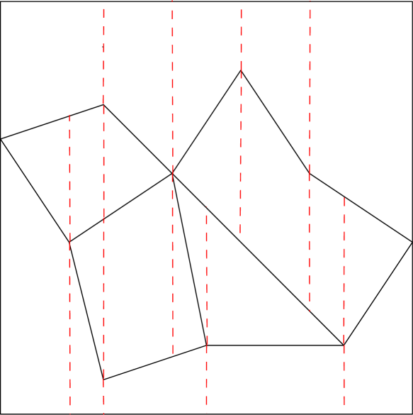
Note that we can assume that the subdivision is enclosed by a bounding box. There are several different ways to solve the planar point location problem optimally in query time and space, see [29] for details. One simple solution uses trapezoidal decomposition, see [19] for a detailed introduction. Roughly speaking, given a planar subdivision enclosed by a bounding box , we construct a trapezoidal decomposition of the subdivision by extending two rays from every vertex of , one upwards and one downwards. The rays stop when they hit an edge in or the boundary of . The faces of the subdivision we obtain after this transform will be only trapezoids. Figure 1 gives an example of trapezoidal decomposition. A crucial property of trapezoidal decomposition is that it increases the complexity of the subdivision by only a constant factor.

We also review some concepts related to cuttings.
Definition 2.3.
Given a set of hyperplanes in the plane, a -cutting, , is a set of (possibly open) disjoint simplices that together cover the entire plane such that each simplex intersects hyperplanes of . For each simplex in the cutting, the set of all hyperplanes of intersecting it is called the conflict list of that simplex.
-cuttings are important in computational geometry as they enable us to apply the divide-and-conquer paradigm in higher dimensions. The following theorem by Chazelle [12], after a series of work in the computational geometry community [24, 25, 6, 7, 14], shows the existence of -cuttings of small size and an efficient deterministic algorithm computing -cuttings.
Theorem 2.1 (Chazelle [12]).
Given a set of hyperplanes in the plane, there exists a -cutting, , of size , which is optimal. We can find the cutting and the corresponding conflict lists in time.
In this paper, we will use intersection sensitive -cuttings which is a generalization of -cuttings. The following theorem is given by de Berg and Schwarzkopf [20].
Theorem 2.2 (de Berg and Schwarzkopf [20]).
Given a set of line segments in the plane with intersections, we can construct a -cutting, , of size . We can find the cutting and the corresponding conflict lists in time using a randomized algorithm.
Note that by the construction of generalized cuttings, see [20] for detail, the following corollary follows directly from Theorem 2.2,
Corollary 2.1.
Given an axis-aligned planar subdivision of complexity , we can construct a -cutting, , of size . More specifically, each cell of the cutting is an axis-aligned rectangle and the size of the conflict list of every cell is bounded by . We can find the cutting and the corresponding conflict lists in time using a randomized algorithm.
2.2 Rectangle Stabbing
In -dimensional rectangle stabbing problem, we are given a set of -dimensional axis-parallel rectangles, our task is to build a data structure such that given a query point , we can report the rectangles containing the query point efficiently. As noted earlier, Chazelle [11] provides an optimal solution in two-dimensions, a linear-sized data structure that can answer queries in time where is the output size. The following lemma by Afshani et al. [3] establishes an upper bound of this problem and it is obtained by a basic application of range trees [8] with large fan-out and Chazelle’s data structure.
Lemma 2.1 (Afshani et al. [3]).
We can answer dimensional rectangle stabbing queries in time using space , where is the number of rectangles, is the output size, and is any parameter.
2.3 A Pointer Machine Lower Bound Framework
We will use the pointer machine lower bound framework of Afshani [1]. The framework deals with an abstract “geometric stabbing problem” which is defined by a set of “ranges” and a set of queries. An instance of the geometric stabbing problem is given by a set of “ranges” and the goal is to preprocess to answer queries . Given , an element (implicitly) defines a subset and the data structure is to output the elements of . However, the data structure is restricted to operate in the (strengthened) pointer machine model of computation where the memory is a directed graph consisting of “cells” where each cell can store an element of as well as two pointers to other memory cells. At the query time, the algorithm must find a connected subgraph of where each element of is stored in at least one memory cell of . The size of is a lower bound on the space complexity of the data structure and the size of is a lower bound on the query time. However, the lower bound model allows for unlimited computation and allows the data structure to have complete information about the problem instance; the only bottleneck is being able to navigate to the cells storing the output elements. In addition, the framework assumes that we have a measure such that . We need a slightly more precise version of the lower bound framework where the dependency on a certain “constant” is made explicit.
Theorem 2.3.
Assume, we have an algorithm that given any input instance of ranges, it can store in a data structure of size such that given any query , it can answer the query in time.
Then, suppose we can construct an input set of ranges such that the following two conditions are satisfied: (i) every query point is contained in exactly ranges and ; (ii) there exists a value such that for any two ranges , is well-defined and is upper bounded by . Then, we must have .
For the proof of this theorem, we refer the readers to Appendix A. In our applications, will basically be the Lebesgue measure and will be the unit cube.
3 Queries on Catalog Paths
In this section, we give a simple solution for when the catalog graph is a path. It will be used as a building block for later data structures.
Theorem 3.1.
Consider a catalog path , in which each vertex is associated with a planar subdivision. Let be the total complexity of the subdivisions. We can construct a data structure using space such that given any query , where is a query point and is a subpath, all regions containing along can be reported in time .
Proof.
We can convert each subdivision into a set of disjoint rectangles of total size using trapezoidal decomposition [19]. Then, we partition into paths, where each path except potentially for has size and has size at most .
Now we use an observation that was also made in previous papers [2, 3, 27]: when , the two-dimensional fractional cascading can be reduced to rectangle stabbing. As a result, for each , , we collect all the rectangles of its subdivisions and build a 2D rectangle stabbing data structure on them. By Lemma 2.1 this requires space. Now given a query subpath of length , we use the rectangle stabbing data structures on the subdivisions of each as long as . Since is a path, for at most two indices we will have and for the rest . This gives us query time. ∎
4 Path Queries on Catalog Trees
Now we consider answering path queries on catalog trees. We first show optimal data structures for trees of different heights. It turns out we need different data structures to achieve optimality when heights differ. We then present a data structure using space that can answer path queries in time and a data structure using space answering path queries in time, where is any constant and is the -th function in the inverse Ackermann hierarchy [18] and is the inverse Ackermann function [18] . We also present lower bounds for our data structures. Without loss of generality, we assume the tree is a binary tree.
4.1 Trees of height
4.1.1 The Upper Bound
For trees of this height, we present the following upper bound. The main idea is to use the sampling idea that is employed previously [9, 3], however, there are some main differences. Instead of random samples or shallow cuttings, we use intersection sensitive cuttings [20] and more notably, the fractional cascading on an arbitrary tree cannot be reduced to a geometric problem such as 3D rectangle stabbing, so instead we do something else.
Lemma 4.1.
Consider a catalog tree of height in which each vertex is associated with a planar subdivision. Let be the total complexity of the subdivisions. We can build a data structure using space such that given any query , where is a query point and is a path, all regions containing along can be reported in time .
Proof.
Let be a parameter to be determined later. Consider a planar subdivision and let be the number of rectangles in . We create an intersection sensitive -cutting on . By Corollary 2.1, contains cells and each cell of is an axis-aligned rectangle. Furthermore, the conflict list size of each rectangle is . For each cell in , we build an optimal point location data structure on its conflict list. The total space usage is linear, since total size of the conflict lists is linear.
Then, we consider every path of length at most in the catalog graph, and we call them subpaths. For every subpath, we collect all the cells of the cuttings belonging to the vertices of the subpath and build a 2D rectangle stabbing data structure on them. Since the degree of any vertex is bounded by , each vertex is contained in at most
many subpaths. Then the total space usage of the 2D rectangle stabbing data structures is bounded by . Given any query path , it can be covered by subpaths. For each subpath, we can find all the cells of the cuttings containing the query point in time and then perform an additional point location query on its conflict list, for a total of query time per subpath. Thus, the query time of this data structure is bounded by
We pick , then we obtain the desired query time. ∎
4.1.2 The Lower Bound
We now present a matching lower bound. We show the following:
Lemma 4.2.
Assume, given any catalog tree of height in which each vertex is associated with a planar subdivision with being the total complexity of the subdivisions, we can build a data structure that satisfies the following: it uses at most space, for a small enough constant , and it can answer 2D OFC queries . Then, its query time must be .
Proof.
We will use the following idea: We consider a special 3D rectangle stabbing problem and show a lower bound using Theorem 2.3. We will use the 3D Lebesgue measure, denoted by . Then we show a reduction from this problem to a 2D OFC problem on trees to obtain the desired lower bound.
We consider the following instance of 3D rectangle stabbing problem. The input rectangles are partitioned into sets of size each. The rectangles in each set are pairwise disjoint and they together tile the unit cube in 3D. The depth (i.e., the length of the side parallel to the -axis) of rectangles in set is . In fact, the rectangles in set can be partitioned into subsets where the projection of the rectangles in the -th subset, , onto the -axis is the interval . See Figure 2 for an example.

We first show the reduction: assume, we are given an instance of the special 3D rectangle stabbing problem described above. We build a balanced binary tree of height on the -axis as the catalog graph. Note that the number of vertices at layer of the tree is the same as the number of subsets in set . We project the rectangles in each subset to the -plane and obtain a 2D axis-aligned planar subdivision. We attach each of the subdivisions to the corresponding vertices. Consider a 2D OFC query, in which is a path that connects the root to a leaf. We lift to a point in 3D appropriately: W.l.o.g., assume the leaf is the -th leaf. To obtain , we assign the coordinate to . By our construct, the -axis projection of any rectangle in the nodes from the root to the leaf contains the coordinate of . This construction ensures that finding the rectangles that contain is equivalent to performing 2D OFC query .
Now we describe a hard instance of the special rectangle stabbing problem to establish a lower bound. It will have rectangles of different shapes. For each shape, we tile (disjointly cover) the unit cube using isometric copies of the shape to obtain a set of rectangles. We collect every different shapes into a class and obtain classes, where is a parameter to be determined later. We say that the -th rectangle in a class has group number , . Now we specify the dimensions (i.e., side lengths) of the rectangles. For a rectangle in class , with group number , its dimensions are
where are parameters to be determined later and the notation denotes an axis-aligned rectangle with width , height , and depth . Observe that every rectangle has volume and thus we need copies to tile the unit cube. By setting , the total number of rectangles we generate is . Also note that all the rectangles in the same group are pairwise disjoint and they together cover the whole unit cube. This implies for any query point in the unit cube, it is contained in exactly rectangles.
Now we analyze the intersection of any two rectangles. First, observe that given two axis-aligned rectangles with dimensions and , their intersection is an axis-aligned rectangle with dimensions at most . Second, by our construction, the rectangles that have identical width, depth, and height are disjoint. As a result, either the width of the two rectangles will differ by a factor or their depth will differ by a factor . This means that, the maximum intersection volume of any two rectangles in class , group can be achieved only in one of the following two cases:
We set , then the intersection volume of any two rectangles is bounded by . However, for the construction to be well-defined, the side length of the rectangles cannot exceed 1 as otherwise, they do not fit in the unit cube. The largest height of the rectangles is obtained for and . Thus, we must have,
By plugging in the values and we get that we must have
| (1) |
Since by our assumptions , it follows that by setting , the inequality (1) holds.
If holds, then we satisfy the first condition of Theorem 2.3 and thus we obtain the space lower bound of
| (2) |
Now observe that if we set , for a sufficiently small , then it follows that the data structure must use more than space. However, by the statement of our lemma, we are not considering such data structures. As a result, when , the query time must be large enough that the first condition of the framework does not hold, meaning, we must have . ∎
4.2 Trees of height
4.2.1 The Upper Bound
We start with the following lemma which gives us a data structure that can only answer query paths that start from the root and finish at a leaf. The main idea here is used previously in the context of four-dimensional dominance queries [3, 9] and it uses the observation that such “root to leaf” queries can be turned into a geometric problem, the 3D rectangle stabbing problem.
Lemma 4.3.
Consider a balanced catalog tree of height , , in which each vertex is associated with a planar subdivision. Let be the total complexity of the subdivisions. We can build a data structure using space such that given any query , where is a query point and is a path starting from the root to a leaf, all regions containing along can be reported in time .
Proof.
Let be a parameter to be determined later. For each subdivision , we create an intersection sensitive -cutting on . By the same argument as Lemma 4.1, all the cells in the cuttings are axis-aligned rectangles satisfying (i) the conflict set size of any cell in is bounded by and (ii) the total number of cells in is .
Now we lift each cell in the cuttings to 3D rectangles and collect all the 3D rectangles to construct a 3D rectangle stabbing data structure for it. This is done as follows. We assign a range for each vertex in the catalog tree; Let be the number of leaves. Order the leaves of the catalog tree from left to right and for the -th leaf , we assign the range as its range. For any internal vertex, its range is the union of the ranges of its children. Then, we lift the 2D rectangles induced by the subdivision of a vertex to a 3D rectangle using the range (i.e., by forming the Cartesian product of the rectangle and the range). We store the 3D rectangles in a rectangle stabbing data structure. Given a query point and a query path , we first lift to be , where is any value in the range of the deepest vertex in , and then query the 3D rectangle stabbing data structure.
In addition, for each cell in a cutting, we build an optimal point location data structure on its conflict set. All these point location data structures take space in total and each of them can answer a point location query in time .
To achieve space bound for the 3D rectangle stabbing data structure, it suffices to choose . We then balance the query time for 3D rectangle stabbing and 2D point locations to achieve the optimal query time
We pick and the query time is bounded by . ∎
The above data structure is not a true fractional cascading data structure because it can only support restricted queries. To be able to answer query paths of arbitrary lengths and , we need the following result.
Lemma 4.4.
Consider a catalog tree in which each vertex is associated with a planar subdivision. Let be the total complexity of the subdivisions and let and , , be two fixed parameters. We can build a data structure using space such that given any query , where is a query point and is a path whose length obeys , all regions containing along can be reported in time .
Proof.
First, observe that w.l.o.g., we can assume that the height of the catalog tree is at most : we can partition the catalog tree into a forest by cutting off vertices whose depth is a multiple of . Since the length of is at most , it follows that can only contain vertices from at most two of the trees in the resulting forest, meaning, answering can be reduced to answering at most two queries on trees of height at most .
Thus, w.l.o.g., assume is the root of the catalog tree of height and is a path of length at least in this catalog tree. We build the following data structures. Let be the vertices at height . Let be the tree rooted at and cut off at height with being leafs and be the tree rooted at , . We build data structures of Lemma 4.3 on and then we recurse on each of the trees. The recursion stops once we reach subproblems on trees of height at most .
Since the data structure of Lemma 4.3 uses space, at each recursive level, the total space usage of data structures we constructed is . Over the recursion levels, this sums up to space.
Now we analyze the query time. Given a query , we may query several data structures that together cover the whole path of . Let be the highest vertex on . We can decompose into two disjoint parts and , that start from and end at vertices and respectively, with and being descendants of . It thus suffices to only answer , as the other path can be answered similarly. The first observation is that we can find a series of data structures that can be used to answer disjoint parts of . The second observation is that we can afford to make the path a bit longer to truncate the recursion. We now describe the details.
Consider the trees defined at the top level of the recursion. If is entirely contained in one of the trees, then we recurse on that tree. Otherwise, is contained in and is contained in some subtree . Now, can be further subdivided into two smaller “anchored” paths: one from to (“anchored” at ) and another from to (“anchored” at ) and each smaller path can be answered recursively in the corresponding tree. Thus, it suffices to consider answering the query along an anchored path.
Thus, consider the case of answering an anchored path in the data structure. To reduce the notation and clutter, assume is an anchored path, starting from the root of and ending at a vertex . Assume the vertices and trees are defined as above. First, consider the case when the height of is at most ; in this case, we have built an instance of the data structure of Lemma 4.3 on but not on the trees . In this case, we simply answer on a root of leaf path in that includes , e.g., by picking a leaf in the subtree of . In this case, we will be performing a number of “useless” point location queries, in particular those on the descendants of . However, as the height of is at most , it follows that the query bound stays asymptotically the same: . Furthermore, there is no recursion in this case and thus this cost is paid only once per anchored path. The second case is when the height of is greater than . In this case, if lies in we simply recurse on but if lies in a tree , we first query the data structure of Lemma 4.3 using the path from the root of until , and then we recurse on . As a result, answering the anchored path query reduces to answering at most one query on an instance of data structure Lemma 4.3 and another recursive “anchored” on a tree of half the height. Thus, the -th instance of the data structure Lemma 4.3 that we query covers at most fraction of the anchored path. Thus, if is the length of the anchored path, it follows that the total query time of all the data structures we query is bounded by
∎
We now reduce the space of the above lemma dramatically. We will repeatedly use a “bootstrapped” data structure. The following lemma establishes how we can bootstrap a base data structure to obtain a more efficient one.
Lemma 4.5.
Consider a catalog tree of height , , in which each vertex is associated with a planar subdivision. Let be the total complexity of the subdivisions. Assume, for any fixed value , , we can build a “base” data structure that can answer a 2D OFC query in time as long as is path of length between and . Furthermore, assume it uses space, for some function which is monotone increasing in and for we have .
Then, for any given fixed value , , we can build a “bootstrapped” data structure that can answer a 2D OFC query in time as long as is path of length between and . Furthermore, it uses space, where is the iterative function which denotes how many times we need to apply function to to reach a constant value.
Proof.
We construct an intersection sensitive -cutting for each planar subdivision attached to the tree. Call these the “first level” cuttings. Similar to the analysis in Lemma 4.1, we obtain cells, which are disjoint axis-aligned rectangles, for each and thus cells in total. Each cell in the cutting has a conflict list of size and on that we build a point location data structure. This takes space in total. We store the cells of the cutting in an instance of the base data structure with parameter . Call this data structure . The space usage of is
Now we consider a query . Let . Consider the case when . In this case, as is built with parameter , we can query it with . Thus, in time, for every subdivision on path , we find the cell of the cutting that contains . Then, we use the point location data structure on the conflict lists of the cells to find the original rectangle containing . This takes an additional as the size of each conflict is . Thus, the query time in this case is
since we have .
Thus, the only paths we cannot answer yet are those when . In this case, we can bootstrap. First, observe that we can build a data structure on the the original rectangles, where is an instance of the base data structure but this time with parameter set to . This will take space. Thus, the total space consumption is
| (3) |
where the last inequality follows since is a monotone increasing function and as . By construction, the data structure is built to handle exactly paths of this length but it is using too much space. The idea here is that we can repeat the previous technique using “second level” cuttings to obtain a data structure : for a subdivision of size , build a -cutting, called the “second level” cutting. By repeating the same idea we used for the first level cuttings, we can spend additional space to build a data structure which can answer queries as long as where . By repeating this process for steps, we can obtain the claim data structure. ∎
We will essentially begin with the data structure in Lemma 4.4 and use Lemma 4.5 to bootstrap. To facilitate the description, we define two useful functions first. Let be the iterated function, i.e., the number of times we need to apply function to until we reach 2. We define as follows
In other words, it is the number of times we need to apply function to until we reach 2. We also defined the following function
In fact, is the -th function of the inverse Ackermann hierarchy [18] and , where the inverse Ackermann function [18].
Lemma 4.6.
Consider a catalog tree of height , , in which each vertex is associated with a planar subdivision. Let be the total complexity of the subdivisions. We can build a data structure using space, where is any constant and is the -th function of the inverse Ackermann hierarchy, such that given any query , where is a query point and is a path of length , , all regions containing along can be reported in time . Furthermore, we can also build a data structure using space answering queries in time , where is the inverse Ackermann function.
Proof.
By Lemma 4.4, if we set and , we obtain a data structure using answering queries in time . By picking , , we can apply Lemma 4.5 to reduce the space to while achieving the same query time. If we again pick , but , by applying Lemma 4.5 again, the space is further reduced to . We continue this process until is less than three. Note that we will need to pay extra query time each time we apply Lemma 4.5. We will end up with a linear-sized data structure with query time . On the other hand, if we stop applying Lemma 4.5 after a constant many rounds, we will end up with a sized data structure with the original query time. ∎
4.2.2 The Lower Bound
We show an almost matching lower bound in this section.
Lemma 4.7.
Assume, given any catalog tree of height , , in which each vertex is associated with a planar subdivision with being the total complexity of the subdivisions, we can build a data structure that satisfies the following: it uses at most space, for a small enough constant , and it can answer 2D OFC queries . Then, its query time must be .
Proof.
We first describe a hard input instance for a 3D rectangle stabbing problem and later we show that this can be embedded as an instance of 2D OFC problem on a tree of height . Also, we actually describe a tree of height . This is not an issue as we can add dummy vertices to the root to get the height to exactly .
We begin by describing the set of rectangles. Each rectangle is assigned a “class number” and a “group number”. The number of classes is and the number of groups is . The rectangles with the same class number and group number will be disjoint, isometric and they would tile the unit cube. Rectangles with class number and group number will be of shape
where are some parameters to be determined later and . Similarly, rectangles with class number and group number will be of shape
The total number of different shapes is . Note that each rectangle has volume , so the total number of rectangles we use in all the tilings is by setting . By our construction any query point is contained in rectangles. Now we analyze the maximal intersection volume of two rectangles. By the same argument as in the proof of Lemma 4.2 the maximal intersection volume can only be achieved by two rectangles when they are in the same class and adjacent groups or in the same group of adjacent classes. For two rectangles and in group of class , we have
We set , then the intersection of any two rectangle is no more than .
We also need to make sure no side length of any rectangle exceeds the side length of the unit cube. The maximum side length can only be obtained when and in the second dimension. We must have
Plugging and in, we must have
| (4) |
Since and , (4) holds.
Suppose , then the first condition of Theorem 2.3 is satisfied and we get the lower bound of
Observe that by setting for a sufficiently small , the data structure must use space, which contradicts the space usage in our theorem. Therefore, .
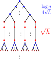
It remains to show that this set of rectangles can actually be embedded into an instance of the 2D OFC problem. To do that, we describe the tree that can be used for this embedding. See Figure 3. We hold the convention that the root of has depth . Starting from the root, until depth , every vertex will have two children (blue vertices in Figure 3) then we will have vertices with one child (red vertices in Figure 3). Then this pattern continues for steps. The first set of blue and red vertices correspond to class , the next to class and so on. Within each class, the top level corresponds to group and so on. To be specific, vertices at depth of the tree have rectangles of class and group . Now, it can be seen that the rectangles can be assigned to the vertices of , similar to how it was done in Lemma 4.2. The notable difference here is that the depth (length of the side parallel to the -axis) of the rectangles decreases as the group number increases from to but then it stays the same from until . This exactly corresponds to the structure of the tree . ∎
4.3 Trees of height
For trees of this height, we have:
Lemma 4.8.
Consider a catalog tree of height in which each vertex is associated with a planar subdivision. Let be the total complexity of the subdivisions. We can build a data structure using space such that given any query , where is a query point and is a path of length , all regions containing along can be reported in time .
Proof.
We combine the classical heavy path decomposition by Sleator and Tarjan [28] and the data structure for catalog paths to achieve the desire query time. We first apply the heavy path decomposition to the tree and then for every heavy path created we build a 2D OFC data structure to answer queries along the path. Clearly, we only spend linear space in total. Then by the property of the heavy path decomposition, we only need to query heavy paths to answer a query, which leads to a query time of . ∎
Corollary 4.1.
Consider a catalog tree in which each vertex is associated with a planar subdivision. Let be the total complexity of the subdivisions. We can build a data structure using space, where is any constant and is the -th function of the inverse Ackermann hierarchy, such that given any query , where is a query point and is a path, all regions containing along can be reported in time . Furthermore, we can also build a data structure using space answering queries in time , where is the inverse Ackermann function.
5 Queries on Catalog Graphs and Subgraph Queries
In this section, we consider general catalog graphs as well as subgraph queries on catalog trees. Our result shows that it is possible to build a data structure of space such that we can save a factor from the naïve query time of iterative point locations. We also present a matching lower bound.
We begin by presenting a basic reduction.
Lemma 5.1.
Given a catalog graph of vertices with graph subdivision complexity and maximum degree , we can generate a new catalog graph with vertices with graph subdivision complexity and bounded degree such that the following holds: given any connected subgraph , in time , we can find a path in such that the answer to any query in equals the answer to query in .
Proof.
The main idea is that we can add a number of dummy vertices to the graph such that we can turn a subgraph query to a path query.
We can obtain in the following way. For every vertex in , place copies of the vertex in . All the copies of a vertex are connected in . Furthermore, every copy of a vertex is connected to every copy of vertex if and only if and are connected in . The maximum degree of is thus .
Now consider a subraph query in . By definition, is a connected subgraph of and w.l.o.g., we can assume is a tree. We can form a walk from by following a DFS ordering of such that traverses every edge of at most twice and visits every vertex of . We observe that we can realize as a path in by utilizing the dummy vertices; as each vertex has dummy vertices, every visit to a vertex in can be replaced by a visit to a distinct dummy vertex. ∎
5.1 The Upper Bound
Formally, we have the following result.
Lemma 5.2.
Consider a degree-bounded catalog graph in which each vertex is associated with a planar subdivision. Let be the total complexity of the subdivisions. We can build a data structure using space such that given any query , where is a query point and is a path, all regions containing along can be reported in time .
Proof.
We build the data structure essentially the same way as in the proof of Lemma 4.1. The only difference is that the degree of a node is bounded by a which can be any constant. By the same argument in the proof of Lemma 4.1, any node is stored at most times and we can obtain a space bounded data structure achieving query time by creating an intersection sensitive -cutting for each planar subdivision and balancing the query time of cutting cells and conflict lists. ∎
By Lemma 5.1, we can also obtain the following two corollaries.
Corollary 5.1.
Consider a catalog graph in which each vertex is associated with a planar subdivision. Let be the total complexity of the subdivisions. We can build a data structure using space such that given any query , where is a query point and is a connected subgraph, all regions containing along can be reported in time .
Specifically, for catalog trees we have the following:
Corollary 5.2.
Consider a catalog tree in which each vertex is associated with a planar subdivision. Let be the total complexity of the subdivisions. We can build a data structure using space such that given any query , where is a query point and is a subtree, all regions containing along can be reported in time .
5.2 The Lower Bound
In this section, we show that the factor that exists in Lemma 5.2, Corollary 5.1, and Corollary 5.2 is tight. Like the proof of path queries for catalog trees, we need a reduction from a rectangle stabbing problem to a 2D OFC subtree query problem on catalog trees. But unlike previous proofs, we use an instance of the rectangle stabbing problem in a much higher dimension. We show the lower bound for subtree queries of a catalog tree. By Lemma 5.1, this also gives a lower bound for path queries in general catalog graphs.
Lemma 5.3.
Assume, given any catalog tree of height in which each vertex is associated with a planar subdivision with being the total complexity of the subdivisions, we can build a data structure that satisfies the following: it uses at most space, for a small enough constant , and it can answer 2D OFC queries , where is a query point and is a subtree containing leaves. Then, its query time must be .
Proof.
We define the following special -dimensional rectangle stabbing problem. The input consists of rectangles in dimensions. According to their shapes, rectangles are divided into sets of size each where is a parameter to be determined later. The rectangles in each set are further divided into groups of size each. All the rectangles in the same group are pairwise disjoint and they together tile the -dimensional unit cube. We put restrictions on the shapes of the input rectangles to make this problem special. For a rectangle in set , , group , , except for the first two and the -th dimensions, its other side lengths are all set to be . The side length of the -th dimension is set to be . We put restriction on the side lengths of the first two dimensions in set as follows: For the first group in this set, we put no restrictions of the first two dimensions as long as they tile the unit cube and the total number of rectangles used for this group is . For an arbitrary group , we cut the range of the unit cube in the -th dimension into equal length pieces. This partitions the unit cube into parts. Note that each part of the unit cube is also tiled by rectangles since we require the side length of the -th dimension of the rectangles to be . If we project the rectangles in each part of the unit cube into the first two dimensions, we obtain axis-aligned planar subdivisions. The planar subdivisions we generated for the first group is used as a blueprint for the shape of rectangles in other groups. More specifically, for the remaining groups in set , we require that the choices of the first two dimensions give the same set of planar subdivisions as the first group. The problem is as follows: Given a point in -dimensions, find all the rectangles containing this query point.
We now describe a reduction from this problem to a 2D OFC subtree query problem on catalog trees. We consider a complete balanced binary tree of height . Note that the number of nodes at layer of the tree is the same as the number of different subdivisions we get by projecting a group in set to the first two dimensions. Since we require that all the groups in the same set yield the same set of subdivisions, we can simply attach the subdivisions to the nodes starting from layer . For nodes in layer smaller than , we attach them with empty subdivisions. Now let us analyze a rectangle stabbing query on the rectangle stabbing problem. Consider rectangles in set , we need to find the rectangle containing in each of the groups. In this special rectangle stabbing problem, to find the rectangle in group containing , we can find the rectangle by first using the -th coordinate of to find the part of the unit cube where is in, and then finding the output rectangle by a simple planar point location on the projection of the part using the first two coordinates of . By our construction this is equivalent to choosing a node in layer of the binary tree and performing a point location query on the subdivision attached to it. Note that the node in layer we choose must be one of the children of the chosen node in layer . So if we only focus on one specific group of all sets, the rectangle stabbing query corresponds to a series of point location queries from the root to a leaf in the binary tree we constructed. Similarly, we obtain such paths if we consider all groups and they together form a subtree of leaves. The answer to the point location queries along the subtree gives the answer to the rectangle stabbing problem.
We describe a hard high dimensional rectangle stabbing problem instance. As before, we create rectangles of different shapes to tile the unit cube. But this time, we will consider a -dimensional rectangle stabbing problem. For rectangles in class , supercluster , we create the following shapes:
where are parameters to be determined later. Note that all the rectangles are in dimensions.
We use each of the shape to tile a unit cube. Since the volume of any rectangle is , we need rectangles of the same shape to tile the cube. We call it a cluster. Note that the rectangles in the same cluster are pairwise disjoint. We generated rectangles in total. By setting , the total number of rectangles is . Note that any point in the unit cube is contained in exactly rectangles.
Now we shall analyze the volume of the intersection between any two -dimensional rectangles. Note that if two rectangles have the same side lengths for out of the last dimensions, then it is the case we have analyzed in the proof of, e.g., Lemma 4.2, and the volume of the intersection of any two rectangles is bounded by if we set . Now we analyze the other case. By our construction, two rectangles can only have at most two different side lengths in the last dimensions. We consider two rectangles in class supercluster , and class supercluster respectively. W.l.o.g., we assume . The case for is symmetric. Then there are two possible expressions for the intersection volume depending on the values of and . The first one is
The second possible expression is
The last inequality holds because .
To make this construction well-defined, no side length of the rectangles can exceed 1. The largest side length can only be obtained in the second dimension when and . We must have
By plugging in the values and we get that we must have
| (5) |
Since by our assumptions , , it follows that by setting , the inequality (5) holds.
If holds, then the first condition of Theorem 2.3 is satisfied and we obtain the lower bound of
Now if we set for a sufficiently small , the data structure must use space, which contradicts the space usage stated in our lemma. Note that . Then . ∎
Remark 5.1.
Note that the lower bound holds even when the query path is of length and . We have already established this lower bound in Lemma 4.2.
Corollary 5.3.
Assume, given any degree-bounded catalog graph in which each vertex is associated with a planar subdivision with being the total complexity of the subdivisions, we can build a data structure that satisfies the following: it uses at most space, for a small enough constant , and it can answer 2D OFC queries , where is a query point and is a path. Then, its query time must be .
6 Open Problems
For the linear space data structure we obtained for general path queries of trees Corollary 4.1, there is a tiny inverse Ackermann gap between the query time we obtain and the lower bound. It is an interesting problem whether we can get rid of that term or improve the lower bound.
The problem we consider is very general in the sense that the only restriction we place on the input instance is that the graph subdivision complexity is . Some special cases admit better solutions. For example, if we require the subdivision complexity of each vertex of the graph to be asymptotically the same, we can obtain an space and query time data structure333This is done by creating an intersection sensitive -cutting for each subdivision in the tree and then storing all cutting cells on each path using the data structure in Theorem 3.1 and building point location data structures on the conflict list of each cell. for path queries on catalog trees of height , which is better compared to the linear space query time data structure we obtained in the general case Lemma 4.1.
Higher dimensional generalization of our results is another direction. In 2D, we can transform an axis-aligned planar subdivision to a subdivision consisting of only rectangles by increasing the subdivision complexity by only a constant factor; however it is not the case for 3D. On the other hand, for 3D point locations on orthogonal subdivisions, we have Rahul’s query time and linear space data structure [27] in the standard pointer machine model. Recently, the query time is improved to by Chan et al. [10], but they use a stronger arithmetic pointer machine model. Given that the higher dimensional counterparts of the tools we use for 2D are suboptimal, it is a challenging and interesting problem to see how the results will be in higher dimensions.
Other open problems include considering the dynamization of our results, i.e., to support insertion and deletion, and other computational models, e.g., RAM and I/O model.
References
- [1] P. Afshani. Improved pointer machine and I/O lower bounds for simplex range reporting and related problems. In Proceedings of the twenty-eighth annual Symposium on Computational Geometry, pages 339–346, 2012.
- [2] P. Afshani, L. Arge, and K. D. Larsen. Orthogonal range reporting: query lower bounds, optimal structures in 3-d, and higher-dimensional improvements. In Proceedings of the twenty-sixth annual symposium on Computational geometry, pages 240–246, 2010.
- [3] P. Afshani, L. Arge, and K. G. Larsen. Higher-dimensional orthogonal range reporting and rectangle stabbing in the pointer machine model. In Proceedings of the twenty-eighth annual Symposium on Computational Geometry, pages 323–332, 2012.
- [4] P. Afshani, T. M. Chan, and K. Tsakalidis. Deterministic rectangle enclosure and offline dominance reporting on the ram. In International Colloquium on Automata, Languages, and Programming, pages 77–88. Springer, 2014.
- [5] P. Afshani, C. Sheng, Y. Tao, and B. T. Wilkinson. Concurrent range reporting in two-dimensional space. In Proceedings of the twenty-fifth annual ACM-SIAM Symposium on Discrete algorithms, pages 983–994. SIAM, 2014.
- [6] P. K. Agarwal. Partitioning arrangements of lines II: Applications. Discrete & Computational Geometry, 5(6):533–573, 1990.
- [7] P. K. Agarwal. Geometric partitioning and its applications. Duke University, 1991.
- [8] J. L. Bentley. Decomposable searching problems. Information Processing Letters, 8(5):244 – 251, 1979.
- [9] T. M. Chan, K. G. Larsen, and M. Pătraşcu. Orthogonal range searching on the RAM, revisited. In Proceedings of the twenty-seventh annual symposium on Computational geometry, pages 1–10, 2011.
- [10] T. M. Chan, Y. Nekrich, S. Rahul, and K. Tsakalidis. Orthogonal point location and rectangle stabbing queries in 3-d. In 45th International Colloquium on Automata, Languages, and Programming, ICALP 2018, page 31. Schloss Dagstuhl-Leibniz-Zentrum fur Informatik GmbH, Dagstuhl Publishing, 2018.
- [11] B. Chazelle. Filtering search: A new approach to query-answering. SIAM Journal on Computing, 15(3):703–724, 1986.
- [12] B. Chazelle. Cutting hyperplanes for divide-and-conquer. Discrete & Computational Geometry, 9(2):145–158, 1993.
- [13] B. Chazelle, H. Edelsbrunner, M. Grigni, L. Guibas, J. Hershberger, M. Sharir, and J. Snoeyink. Ray shooting in polygons using geodesic triangulations. Algorithmica, 12(1):54–68, 1994.
- [14] B. Chazelle and J. Friedman. A deterministic view of random sampling and its use in geometry. Combinatorica, 10(3):229–249, 1990.
- [15] B. Chazelle and L. J. Guibas. Fractional cascading: I. a data structuring technique. Algorithmica, 1(1-4):133–162, 1986.
- [16] B. Chazelle and L. J. Guibas. Fractional cascading: II. applications. Algorithmica, 1(1-4):163–191, 1986.
- [17] B. Chazelle and D. Liu. Lower bounds for intersection searching and fractional cascading in higher dimension. Journal of Computer and System Sciences, 68(2):269–284, 2004.
- [18] T. H. Cormen, C. E. Leiserson, R. L. Rivest, and C. Stein. Introduction to algorithms. MIT press, 2009.
- [19] M. de Berg, O. Cheong, M. van Kreveld, and M. Overmars. Computational Geometry: Algorithms and Applications. Springer-Verlag, 3 edition, 2008.
- [20] M. de Berg and O. Schwarzkopf. Cuttings and applications. International Journal of Computational Geometry & Applications, 5(04):343–355, 1995.
- [21] M. de Berg, M. van Kreveld, and J. Snoeyink. Two-and three-dimensional point location in rectangular subdivisions. In Scandinavian Workshop on Algorithm Theory, pages 352–363. Springer, 1992.
- [22] P. F. Dietz and R. Raman. Persistence, amortization and randomization. In Proceedings of the second annual ACM-SIAM symposium on Discrete algorithms, page 78–88, 1991.
- [23] Y. Giyora and H. Kaplan. Optimal dynamic vertical ray shooting in rectilinear planar subdivisions. ACM Transactions on Algorithms, 5(3), 2009.
- [24] J. Matoušek. Cutting hyperplane arrangements. Discrete & Computational Geometry, 6(3):385–406, 1991.
- [25] J. Matoušek. Approximations and optimal geometric divide-and-conquer. Journal of Computer and System Sciences, 50(2):203–208, 1995.
- [26] K. Mehlhorn and S. Näher. Dynamic fractional cascading. Algorithmica, 5(2):215–241, 1990.
- [27] S. Rahul. Improved bounds for orthogonal point enclosure query and point location in orthogonal subdivisions in . In Proceedings of the twenty-sixth annual ACM-SIAM Symposium on Discrete Algorithms, pages 200–211. SIAM, 2014.
- [28] D. D. Sleator and R. E. Tarjan. A data structure for dynamic trees. Journal of Computer and System Sciences, 26(3):362–391, 1983.
- [29] C. D. Toth, J. O’Rourke, and J. E. Goodman. Handbook of discrete and computational geometry. CRC press, 2017.
Appendix A Proof of Theorem 2.3
See 2.3 To prove this theorem, we first show a special property of the subgraph explored to answer a query . Note that in the pointer machine model, we begin the exploration with a special cell, called the root. If we consider only the first in-edge to any cell in , we obtain a tree.
Lemma A.1.
Let be the explored subgraph corresponds to a query . We call the memory cells in containing reported ranges marked cells. Let a fork be a subtree of of size at most containing two marked cells, where is a large enough constant and is the parameter in Theorem 2.3. Then can be decomposed into many forks, where is the set of ranges containing .
Proof.
The proof we present is very similar to the one described in [1]. We generate the forks using the following method. For every cell in , we assign two values mark and size to it. For marked cell, we initialize its mark value to be one. Other cells will have mark value zero. For any cell in , we assign one to its size value. Without loss of generality, we assume to be a tree. At every step, we choose an arbitrary leaf and add its mark value and size value to the corresponding values of its parent. Then we remove this cell. If its parent has another child, we repeat this process until its parent becomes a leaf. If after this process its parent has mark value two and size value more than , we remove its parent as well and do nothing. We call this situation “wasted”. If its parent has mark value two and size value no more than , we find a fork. We add it to the fork set and remove the subtree. If its parent has mark value less than two, we do nothing. Note that its parent cannot have mark value more than two because that will indicate one of its child has mark value at least two but not being added to a fork or wasted. We go on to the next step until reaching the root.
Let us consider how many marks will be wasted. We only waste marks when we find a subtree containing two marks but of size more than and when we reach the root with only one mark. Since contains cells, the number of marks wasted is bounded by . Other marks are all stored in forks, so the number of forks is more than for a sufficiently large . ∎
We also need another lemma, which follows directed from Lemma 1 in Afshani [1].
Lemma A.2.
The number of forks of size is .
Now we prove Theorem 2.3.
Proof.
Consider any query point . By definition, it is contained in a set of ranges. Consider the explored subgraph when answering . By Lemma A.1, we can decompose into a set of forks such that each fork contains two output ranges. Note that for the two ranges to be output, must lie in the intersection of the two ranges. Similarly, must lie in all the intersection of the two ranges for every fork in . This implies that is covered by these intersections times.
Since we can answer queries for all and by assumption (i) each is contained in ranges, it implies that the intersections of two ranges in all possible forks cover times. By Lemma A.2, the number of possible forks of size is . Each fork has ways to choose two ranges. By assumption (ii), the measure of any two ranges is bounded by . So by a simple measure argument,
This gives us
By our assumption (i), , we also obtain
∎