Wavefront Shaping with a Tunable Metasurface: Creating Coldspots and Coherent Perfect Absorption at Arbitrary Frequencies

Abstract

Modern electronic systems operate in complex electromagnetic environments and must handle noise and unwanted coupling. The capability to isolate or reject unwanted signals for mitigating vulnerabilities is critical in any practical application. In this work, we describe the use of a binary programmable metasurface to (i) control the spatial degrees of freedom for waves propagating inside an electromagnetic cavity and demonstrate the ability to create nulls in the transmission coefficient between selected ports; and (ii) create the conditions for coherent perfect absorption. Both objectives are performed at arbitrary frequencies. In the first case a novel and effective optimization algorithm is presented that selectively generates coldspots over a single frequency band or simultaneously over multiple frequency bands. We show that this algorithm is successful with multiple input port configurations and varying optimization bandwidths. In the second case we establish how this technique can be used to establish a multi-port coherent perfect absorption state for the cavity.

I Introduction

Extreme electromagnetic environments are prevalent in much of our day to day lives. While often unnoticed, this puts significant stress on the design of electronic systems that are expected to work under all conditions. Extraordinary care is taken to counter adverse effects whenever possible, but the operating environment is rarely known ahead of time. In addition, Electromagnetic Interference (EMI) takes the form of unwanted coupling between components. Some platforms, such as aircraft and spacecraft, can experience devastating consequences, resulting in severe mission degradation or even casualties [1]. Wave fields in electrically large enclosed areas such as passenger compartments in transportation systems show extreme sensitivity to frequency and geometric details even though these enclosures, termed chaotic cavities, are not intended to be reverberant. In such cavities the electromagnetic wave fields have specific statistical properties that depend upon a limited number of parameters [2]. Among these is the fact that the wave field is statistically equivalent to a random superposition of plane waves [3]. As such, we can leverage analytical tools from the active research area of quantum chaos [4, 5] in the more generalized framework of wave chaos [6].

Our goal is to adaptively and intelligently control fields inside complex electromagnetic environments. We show that this can be achieved through programmable metasurfaces, which increase the available Degrees of Freedom (DOF) by manipulating boundary conditions [7, 8, 9]. In recent years, these devices have enabled novel concepts in a wide variety of applications throughout the microwave and optical domains [10, 11, 12, 13, 14, 15, 16]. The additional DOF in turn enhance diversity in space and time [17, 18, 19, 20], and allow intricate control of the underlying scattering system; combining a programmable metasurface with a cavity unlocks applications not possible with a fixed system [21, 22, 23] and encourages research in new and under-explored domains [24].

One such unexplored area is Coherent Perfection Absorption (CPA), where coherent excitation of a lossy system can result in complete absorption of all incident waves [25, 26]. It has applications in highly efficient notch filtering, energy conversion, and even detection; since the CPA state is extremely sensitive to parameter variation, it can be used to identify small changes in a complex scattering system [27]. The ability of a metasurface to manipulate additional DOF presents a novel capability for realizing CPA states.

In this article we describe the use of a binary programmable metasurface to create microwave coldspots at arbitrary frequencies, and to realize CPA states, both within the 1 GHz band of operation of the metasurface. The conceptual overview is shown in Figure 1 where the metasurface is installed in a complex reverberating cavity and controlled in a closed loop manner. Input directional diversity is introduced by simultaneously driving multiple ports with arbitrary relative phase shifts. An iterative optimization algorithm is used to generate coldspots at the output port, or to drive candidate scattering matrix eigenvalues towards the origin to achieve CPA.

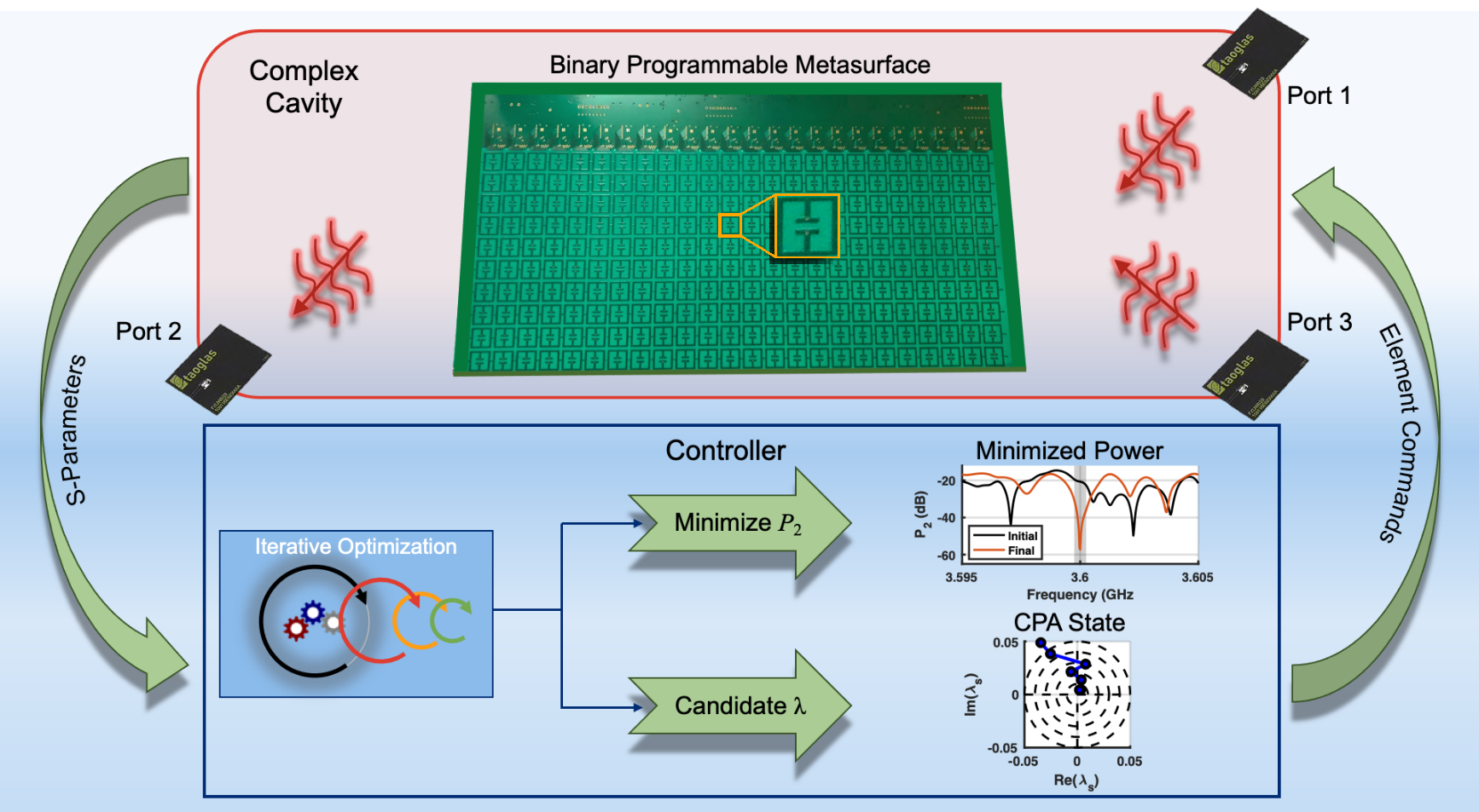
Figure 1: Conceptual overview of the metasurface enabled cavity as a closed loop system. The cavity $S$-parameters (scattering parameters) are measured with a network analyzer and passed to a controller that updates the metasurface elements with a new set of commands. The controller can generate coldspots at port 2 at an arbitrary set of frequencies, or drive candidate $S$-matrix eigenvalues towards the origin, and includes a stochastic iterative optimization algorithm. The three ports allow additional angular and spatial diversity to be added at the inputs. The inset shows a closeup view of one of the metasurface unit cells.

II Cavity Configuration

The metasurface used for this work is a reflectarray fabricated by the Johns Hopkins University Applied Physics Laboratory (JHU/APL) that is designed to operate from 3-3.75 GHz. It has a lattice of $10\times 24$ squares occupied by unit cells with size $<\lambda/6$ [28], where $\lambda$ is the wavelength. These 240 unit cells can be independently set to one of two states, which approximate electric or magnetic boundary conditions and provide a relative 180^∘ phase shift for waves reflected by the element. This results in the local surface impedance of the array varying from cell to cell and state to state. The array surface thus has $2^{240}$ independent states, each of which reflects waves in a uniquely different set of directions. We refer to the settings of the 240 elements as a command.

As shown in Figure 2, the array was installed in a 0.76 m³ cavity where it covers $\sim 1.5\%$ of the total interior surface area. The cavity has 3 ports with one acting as a target for scoring and two used for signal injection; the input ports can be driven either individually or collectively with a relative phase shift. Although 3 ports are present, we are typically using the cavity as a 2-port system because we have a 2-port network analyzer. All 3 ports are used when driving ports 1 and 3 simultaneously, in which case the underlying scattering system is represented by a $3\times 3$ scattering matrix. While the experiment has a physically fixed number of ports, the results can be generalized to an arbitrary number of ports. The cavity has both low and high loss configurations to test how the behavior varies with the typical quality factor, $Q$, of the modes; here we consider the high $Q$ case. Introducing the metasurface to the cavity reduced the average $Q$ in the frequency band of operation of the metasurface by a factor of $\sim$2. However, once the metasurface was installed, the average $Q$ was found to be independent of the number of active or inactive elements on the surface. The quality factor was determined to be roughly $5.5\times 10^{3}$, by measuring the power decay time, $\tau=Q/\omega$ (250 ns with the metasurface installed). Further details of the metasurface, cavity construction, experimental setup, and impact of the metasurface on losses are provided in the supplemental material.

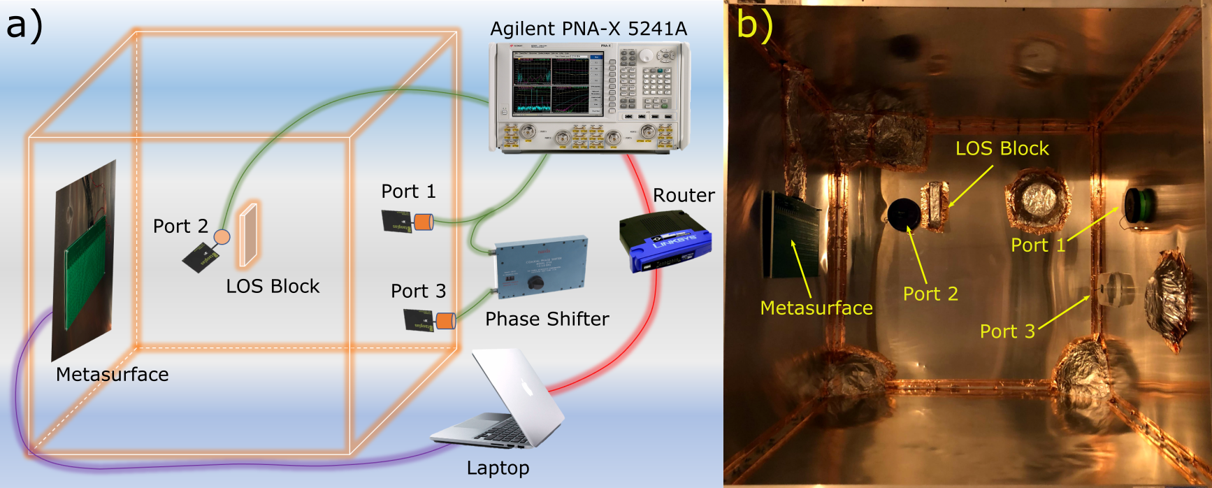
Figure 2: Experimental schematic and cavity configuration. a) Schematic of the experimental setup in the configuration driving all 3 ports. A network analyzer (Agilent PNA-X 5241A) is used to measure cavity $S$-parameters, with channel 1 connected to both Port 1 and Port 3 (through a phase shifter) and channel 2 connected to Port 2. The ports are terminated with ultra wideband antennas. The metasurface is mounted on the cavity wall opposite Ports 1 and 3, and a block is used next to Port 2 to break the line of sight (LOS) between Port 2 and Ports 1 and 3. A laptop controls the system and is connected to the metasurface through a USB interface and to the network analyzer through a wired ethernet link. b) Photograph looking inside the cavity, with the metasurface and ports labeled. Also shown in the photo are the line of sight block and the irregular scattering elements installed on the cavity walls as discussed in the supplemental material.

The cavity mean mode spacing in frequency, $\Delta f$, is found from the Weyl formula as $\Delta f=\pi c^{3}\left(2\omega^{2}V\right)^{-1}$ [29]. A measure of the loss in the cavity is the $Q$-width of a mode normalized to the mode spacing, $\alpha=f/(2\Delta fQ)=3$ for this cavity. For our cavity, the mean mode spacing is roughly 115 kHz at a 3.5 GHz center frequency. As discussed in the supplemental material, the mean spacing between nulls in the transmission coefficient, $|S_{21}|$, was found to be $\sim$2 MHz and the average width of the nulls was found to be $\sim$200 kHz. This indicates a transmission coefficient null contains about 2 modes. Alternatively, it corresponds to a path difference of 750 m between two interfering signals.

We are interested in the steady state response, so the average $Q$ does put a bound on the effective speed with which we can switch the cavity scattering matrix between fixed states. This can be seen through the power decay time, which measures how quickly energy in the cavity dissipates. In order to guarantee a steady state result, the metasurface commands must be toggled at a rate slower than $1/\tau$. The time between measurements must also be staggered by several $\tau$ to ensure each measurement corresponds to the desired metasurface commands. To observe transient behavior in a cavity with a 250 ns power decay time, the metasurface commands must be switched at rates greater than 4 MHz. This assumes the bandwidth of the measured phenomena is wider than the switching rate; an additional complication arises with narrow bandwidth responses that are of interest. When considering finite bandwidth nulls (200 kHz as stated above), the narrower bandwidth process will determine the bound. Our experimental setup is limited to switching rates $<$ 1 Hz, so neither limit presents a practical concern for our configuration. However, experiments with an embedded microcontroller demonstrated that the metasurface itself can be switched at rates up to 15 kHz [28], so this may need to be considered with high speed operation in higher $Q$ cavities.

A complex scattering system such as our cavity exhibits both universal fluctuations, which can be described by Random Matrix Theory (RMT) [4], and deterministic behavior arising from the system specific configuration of the ports and short orbits between the ports [30, 31, 32]. Due to the small relative size of the metasurface, the chaotic ray paths with many multipath bounces will experience the strongest influence. Since minimizing the power received at a port is accomplished by creating destructive interference of the ray paths, the relationship between commands and responses is quite complicated. This leads to utilizing stochastic iterative approaches, or machine learning, in place of linear deterministic methods for control. Here we consider iterative processes. A metasurface covering a larger fraction of the interior surface would likely produce stronger results [33] and allow us to use a transmission matrix based approach to determine the optimal metasurface commands [34, 35, 36]. For this reason most prior research utilizes metasurfaces that cover a significant portion of a wall (or multiple walls). However, using a relatively small metasurface coverage is better suited for real world applications where it is not practical to build or use a larger device.

A key step in evaluating system performance is to determine the range of possible responses of the scattering properties of the system so as to ensure that we have a sufficiently diverse command set. Unfortunately, with $2^{240}$ possible commands (approximately $1.8\times 10^{72}$), it is not feasible to test every one and we need to find a reduced number that produces the full range of outcomes. As discussed in the supplemental material, deterministic decomposition of commands into orthogonal basis functions, such as Hadamard bases [37, 38], generated a very narrow range of system scattering responses. Diversity in the responses requires a distribution of commands with a variety of spatial frequencies, ratios of active to inactive elements, and localized groupings of active elements. Doubly random methods or compound distributions, such as a biased coin toss, or power law spectral density with the bias, or power exponent itself a random draw, were found to yield the widest range of responses. Details of our novel stochastic algorithm are discussed in the next section and the supplemental material.

III Generating Coldspots

Our goal is to program the metasurface to minimize the transmission between two ports in a complex scattering system at an arbitrary frequency. Cases are scored by evaluating the difference in average power, $\Delta P_{2}$, in a specified frequency range at a given center frequency between the initial inactive (all 0s) state and the current state of the metasurface. To maximize this difference we take a directed random walk approach in which at each step a number of array element states are toggled (changed), $\Delta P_{2}$ is evaluated, and the new state is accepted or rejected based on whether or not it decreases $\Delta P_{2}$. As discussed in the previous section, we need to have a mix of large and small spatial groupings of elements and a varied number of active elements to ensure a diverse set of responses. To meet this requirement, our iterative algorithm operates in 2 distinct phases: multiple element toggling and individual element toggling.

In the multiple element toggling phase, we select $M$ elements at random as a trial and toggle their state ($0\rightarrow 1$ and $1\rightarrow 0$). If $\Delta P_{2}$ is decreased, the trial set of commands becomes the new reference set and we repeat the process selecting another $M$ elements at random and toggling their state. When $T$ consecutive trials have been made without improving $\Delta P_{2}$ we claim convergence and move to the next value of $M$. In a typical experimental run, $M=[120,48,24,12,6]$, and $T$ = 30. After all values of $M$ have been exhausted, we move to the individual element phase.

The individual element toggling phase has 3 cases associated with each trial. We select a single element at random and toggle it and then, in an adaptation of the neighbor toggling method of Ref. [39], we toggle the 4 nearest neighbors and the 4 diagonal neighbors. $\Delta P_{2}$ is evaluated for each of these cases and the algorithm continues as in the 1st phase until $T$ consecutive trials are performed without improving $\Delta P_{2}$.

The multiple element toggling phase tends to result in a local minimum which is difficult to escape when toggling only a single element. Adding neighbor toggling significantly improves the performance, as it provides larger localized changes in the command set and allows us to escape the local minimum. Even with the neighbor toggling, however, our stochastic approach does not guarantee that a global minimum is found. Increasing the convergence criteria, $T$, can increase the probability of finding the global minimum, but comes with the cost of increased time. The absolute minimum is not necessarily required, and our stochastic algorithm is able to provide substantially deep nulls at arbitrary frequencies in a reasonable amount of time.

A typical experimental run will provide $\sim$350 trials, $\sim$25 iteration updates, and take $\sim$1.5 hours, as the experimental setup is not optimized for run time. We use an ethernet connection to transfer 32001 frequency samples over the full 1 GHz band for each of the 4 complex $S$-parameter measurements using 64-bit precision. With the frequency values themselves included, this means 2.3 MB of data are transferred for each trial. In addition, the commands and measured $|S_{21}|$ are plotted at each trial for operator feedback, resulting in a delay of $\sim$15 seconds per trial. Disabling plotting and capturing only the processed frequency band could potentially reduce the time to 1-2 seconds per trial, or 6-12 minutes for an experimental run. In general, the cavity should not be used for other purposes while generating a coldspot, as trials that move in the wrong direction in the solution space may produce undesirable responses. Reducing the time to find a solution in only a few minutes may present an acceptable interruption in service. To move towards a faster, real time operational system, we would replace the network analyzer with software defined radios (SDRs), such as the HackRF One [40] or BladeRF [41] commercial devices which retail for $\sim$$300 or $\sim$$500-1000 respectively. In addition, an embedded micro-controller, such as an Arduino or Raspberry Pi, could be used to reduce the USB communications overhead induced by traditional desktop operating systems when interfacing with the metasurface. This would mean measuring signal I and Q channels rather than $S$-parameters; however, this is a realistic requirement for a practical fielded solution that would not use a bulky, expensive network analyzer anyway. Trial rates approaching 1 kHz could be achieved in this fashion, though substantial engineering effort would be required to reduce the latency to approach the metasurface switching limit of 15 kHz [28].

Figure 3 shows the results obtained when minimizing the average power at the output port and compares the results of many different experiments and configurations. All the cases are scored by the change in average power, $\Delta P_{2}$, between the initial inactive (all 0s) state and the final state. The optimization algorithm was performed with $\Delta P_{2}$ evaluated over a single frequency band as well as simultaneously over multiple separated frequency bands. As discussed previously, the widths of the nulls were observed to be $\sim$200 kHz. The initial bandwidth was selected to be 500 kHz in order to ensure that $\Delta P_{2}$ was evaluated over an entire null. In addition, the cavity configuration was switched between driving a single input port and driving two input ports simultaneously with varying relative phase shifts. The achieved suppression ranges from 4-40 dB with most cases providing $>$ 10 dB. The lower values of $\Delta P_{2}$ arise in the following cases: working near the edges of the metasurface operational window, evaluating $\Delta P_{2}$ over a large bandwidth, or evaluating $\Delta P_{2}$ over multiple separated bands. This is not surprising as more bandwidth results in more features in the region where $\Delta P_{2}$ is evaluated, which then means more degrees of freedom are required to be manipulated for destructive interference. The metasurface provides some benefit outside of the 3-3.75 GHz design window; the reflection phase change of the pixels is limited near the edges of the operational bandwidth, so performance is expected to be reduced under those conditions. More details on specific cases are provided in the supplemental material.

Since $\Delta P_{2}$ is inherently a relative measurement, there is an implicit dependence on the initial state. Using the inactive (all 0s) state as the reference ensures the metasurface is always initialized with the same command even though the specific value is dependent on the selected frequency window. Starting with a condition where there was already a deep null would result in limited improvement; the average power in that case would already be quite low and there would not be a need for further reduction. Starting with a condition where there is a transmission peak however, would result in significant reduction. When using a single frequency band metric, we were able to drive deep nulls in each of the windows that were tested, as can be seen by the circles in Fig. 3a and the power at port 2 in panels b) through e). Panels b) and d) show moderate cases where there is not a clear peak in the initial $P_{2}$ measurement, while panels c) and e) show cases with a clear peak in the initial $P_{2}$ measurement and demonstrate significant improvement. This highlights the dependence of $\Delta P_{2}$ on the initial state.

Deep transmission nulls were also observed when driving two input ports simultaneously with varying relative phase shifts, as shown by the diamonds in Fig. 3a. This indicates our approach is self-adaptive and can compensate for multiple input signals as well as signals coming in from different directions. With dual frequency bands however, we were generally unable to drive deep nulls in both bands simultaneously, which can be seen by the hexagrams in Fig. 3a and the power at port 2 over the frequency band in panels f) and g). This is because the metasurface frequency response in separated bands is correlated, as the metasurface induces wide bandwidth effects on the scattering properties of the enclosure. As shown in the supplemental material, different choices of metrics produce different out of band behavior. These results show that our approach provides 3 distinct advantages over previous works: 1) we are able to generate coldspots at arbitrary frequencies and are not limited to a single operating frequency; 2) we are able to generate coldspots simultaneously in multiple separated frequency bands as well as at single frequencies; and 3) we are able to generate coldspots when the injected signal comes from multiple directions with an arbitrary relative phase shift and are not limited to a single direction.

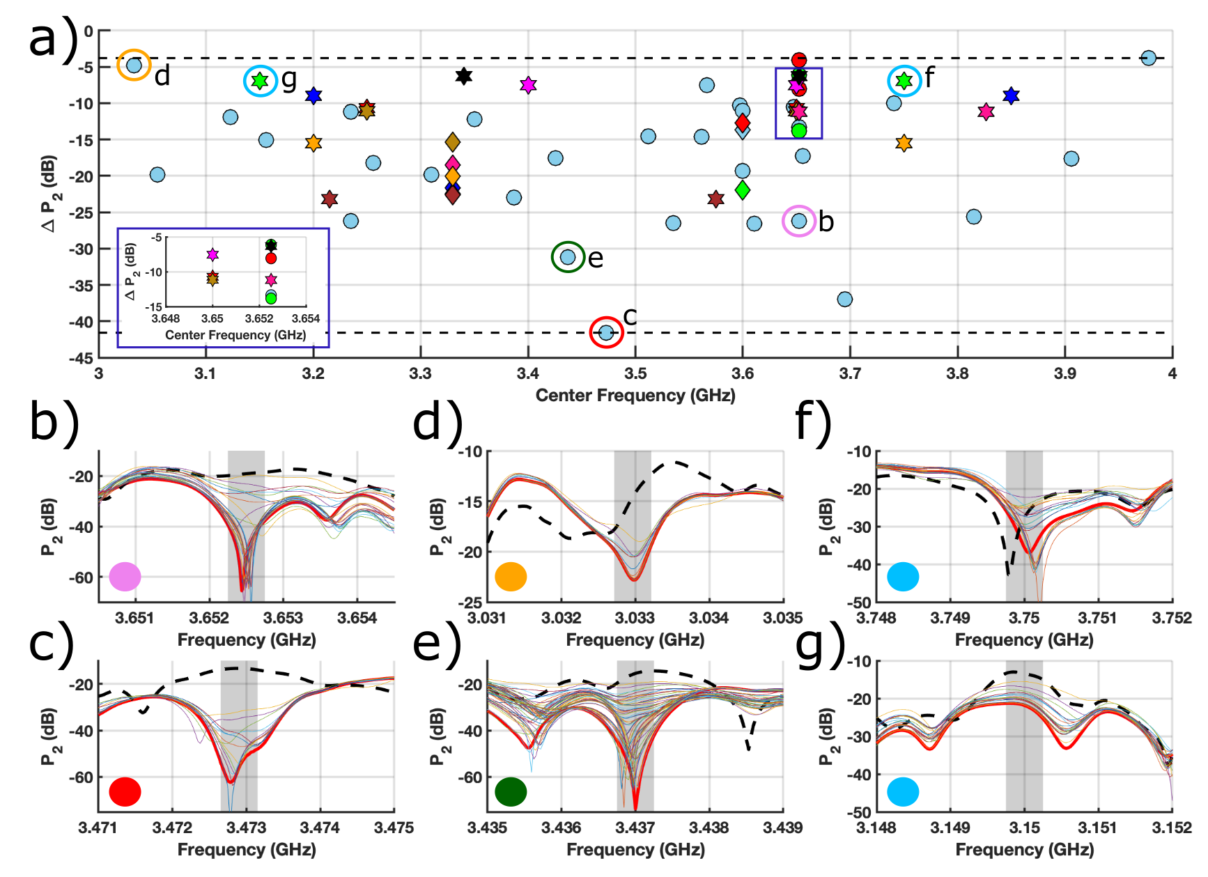
Figure 3: Results of minimizing power at port 2 with the iterative optimization algorithm. a) Plot of $\Delta P_{2}$ at various frequencies in the range of operation of the metasurface. Circles represent cases where the metric was evaluated over a single frequency band and are color coded by bandwidth (sky blue is 500 kHz, green is 5 MHz, and red is 10 MHz). Hexagrams represent dual frequency band metrics and are color coded by matching pairs. Diamonds represent driving both ports 1 and 3 collectively and are color coded by relative phase shift (0, 8, 15, 25, and 50 deg/GHz). Letters indicate points shown in detail in the following panels. The dashed black lines indicate the smallest reduction (-4dB) and largest reduction (-41 dB). b through g) $P_{2}$ evolution from initial (all 0s) to final state. The dark shaded region represents the frequency band where $\Delta P_{2}$ was evaluated, the dashed black line shows the initial response, the solid bold red line shows the final response, and the remaining lines show a few of the incremental steps. b and c) Single band examples centered at 3.033 GHz and 3.6525 GHz, with 28 and 5 dB of suppression, respectively. d and e) Single band examples centered at 3.473 GHz and 3.437 GHz, with 41 and 31 dB of suppression, respectively. f and g) Dual band example centered at 3.75 GHz and 3.15 GHz, with 7 dB of suppression averaged over the 2 bands.

IV Generating Coherent Perfect Absorption

Coherent Perfect Absorption (CPA) is a situation in which all energy injected into a system is absorbed, no matter how small the losses are in the system. Creating CPA requires coherent excitation of all the ports in an eigenvector whose corresponding $S$-matrix eigenvalue is zero. Operationally, the first step in establishing CPA is to find an eigenvalue of the scattering matrix that is close to zero. For example, a 2 x 2 scattering matrix will have a pair of eigenvalues at each frequency. However, realizing CPA only requires driving 1 eigenvalue to zero, as the other eigenvalue corresponds to the anti-CPA state [27]. For the following discussion and experimental results, we only consider the smallest eigenvalue of each pair.

CPA has typically been investigated in simple, regular scattering scenarios and cavities but recently it has been demonstrated in more complex systems, specifically in the realm of wave chaos, and graphs [42, 43, 44, 45]. These works analytically demonstrate the use of RMT to explore CPA states with semiclassical tools without relying on the limit of weak coupling. CPA states have also been experimentally investigated in multiple scattering environments [26], and in graphs that break time-reversal invariance [27]. The use of enhanced spatio-temporal diversity from a metasurface for realization of CPA has not yet been explored.

Recent research however has investigated the use of metasurfaces for Perfect Absorption (PA) inside a cavity and demonstrated a secure communication system as an application [46]. PA is a complementary idea to CPA for a single port system that relies only on the reflection coefficient, $S_{11}$ [47]. Coherent excitation of a single port with complete absorption has been demonstrated to enhance wireless power transfer [48]. Our work extends this to coherent operation with the full scattering matrix for a 2-port system, and can be generalized to an arbitrary number of ports.

Realizing a true absolute zero of the $S$-matrix eigenvalues is generally difficult, because the eigenvalues are complex numbers. Thus two parameters must be varied independently to drive an eigenvalue to zero. Further, a CPA state is highly dependent on the structure of the underlying scattering system. This is best understood in the framework of the Random Coupling Model (RCM) [6, 49]. The eigenvalues accessible by means of the programmable metasurface tend to cluster around values determined by the coupling properties of the ports, which are characterized by the radiation $S$-matrix, $S_{\text{rad}}$. We define $S_{\text{rad}}$ as the $S$-matrix corresponding to the free-space radiation condition with the cavity walls taken out to infinity such that no waves come back to the ports [50]. $S_{\text{rad}}$ can be determined by a number of means [51]. Here we employ the ensemble average of the time gated measured $S$-parameters in the cavity [29], as described in the supplemental material. Deviations of the scattering matrix from $S_{\text{rad}}$ have a number of causes. First there are deviations resulting from relatively direct ray paths between the ports [31]. These deviations are removed by averaging the $S$-matrix over a frequency window that is the reciprocal of the time of flight on the path. However, in finding the eigenvalues of the $S$-matrix in a narrow frequency range, these deviations are present. Second, there are deviations due the multitude of longer paths, and these are characterized statistically by RMT within the RCM. These fluctuations in $S$ tend to be of the order of $1/(\pi\alpha)^{1/2}$ [30, 31, 32] where the loss parameter $\alpha=f/(2\Delta fQ)=3$ in the present experimental case. Finally, there are deviations dependent on the state of the metasurface. These deviations are constrained to be less than or equal to either the direct path or the statistical long path deviations.

Thus, to find a CPA state it is necessary for the ports to be sufficiently matched so that the statistical fluctuations can shift the eigenvalues to zero. If the ports are poorly matched and losses within the cavity are sufficiently high, the eigenvalues will naturally fall near values determined by the properties of the ports with statistical fluctuations around those values dictated by the amount of cavity loss. As such, it is generally not possible to realize a CPA state at arbitrary frequencies when limited to a single DOF [27]. The availability of additional DOF, such as those produced by the metasurface, allows greater control over the underlying scattering system and provides a greater likelihood of potential CPA states.

Characterization of the $S$-matrix eigenvalues from a distribution of 2000 command sets is presented in Figures 4 and 5. Figure 4 shows the probability distributions for all of the $S$-matrix eigenvalues over all frequencies and commands. Panel a) shows that the magnitude follows a Rician distribution as predicted by Ref. [52], which also tells us that the $\nu$ parameter of the Rician distribution is due to the presence of persistent short orbits [53]. Panel b) shows that the phase of the $S$-matrix eigenvalues is not truly uniformly distributed. The deviation of the eigenphase from uniformity indicates that the random distribution is not statistically independent and again tells us there are persistent short orbits present in the system. These short orbits are not captured explicitly in $S_{\text{rad}}$, and will cause the eigenvalues of $S_{\text{rad}}$ to be offset from the center of the point cloud of $S$-matrix eigenvalues. Short orbits can be explicitly included analytically in the RCM [53, 54] and do not prevent us from proceeding. Panel c) shows the CDF of the eigenvalue magnitudes and is useful in establishing thresholds for potential CPA candidates.

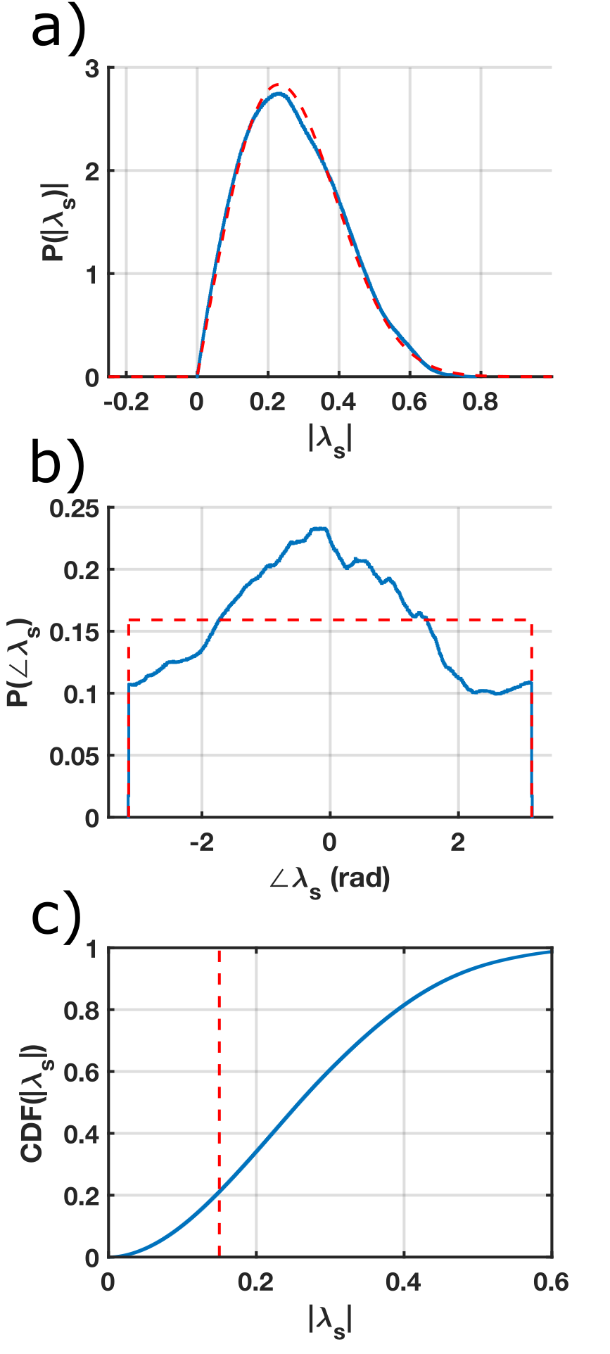
Figure 4: $S$-matrix statistics for a random distribution of 2000 metasurface commands. Panels show statistics for the scattering matrix eigenvalues covering all commands and all frequencies from 3-4 GHz. a) PDF for the magnitude of scattering matrix eigenvalues, $|\lambda_{s}|$. The dashed red line shows the fit to a Rician distribution with $\sigma$ = 0.173 and $\nu$ = 0.177. b) PDF for the phase of scattering matrix eigenvalues, $\angle\lambda_{s}$. The dashed red line shows the distribution for a perfectly uniform phase. c) CDF for the magnitude of scattering matrix eigenvalues. The dashed red line shows the threshold of $|\lambda_{s}|<$ 0.15.

Figure 5 shows point clouds of the $S$-matrix eigenvalues at selected frequencies and demonstrates that the eigenvalues can have very different behavior in how they approach the origin. The panels show the collection of eigenvalues of the 2000 $S$-matrices at selected frequencies along with the eigenvalues of $S_{\text{rad}}$ at that frequency. We can see that the eigenvalues of the distribution tend to cluster around the eigenvalues of $S_{\text{rad}}$; the offset from the center of the point cloud is due to the presence of short orbits, as discussed above. In panel a), the $S$-matrix eigenvalues are clustered in the upper right quadrant far from the origin and do not enter the inner rings. The $S_{\text{rad}}$ eigenvalue is in the upper right-hand quadrant outside of the plot area, at $0.1862+j0.2288$. In panel b), the $S$-matrix eigenvalues are clustered in the upper half, with some getting close to the origin. In panel c), the $S$-matrix eigenvalues show a fairly uniform density throughout the full $|\lambda_{s}|<$ 0.15 range. In panel d), the $S$-matrix eigenvalues show a high density clustered around the origin. The results in these panels are from a random distribution of commands rather than a targeted search. During optimization, we will take smaller dithering steps for finer control as we approach the origin, and expect to see slightly different behavior.

The variance in eigenvalue magnitudes means we need to use a large threshold for identifying candidates because the overall global minimum $S$-matrix eigenvalue may not be identified as a candidate in every realization. In practice, we found that we were unable to realize CPA states when starting with a magnitude $|\lambda_{s}|\geq$ 0.2 but were generally able to realize CPA states when starting with a magnitude $|\lambda_{s}|\leq$ 0.15. Moving an eigenvalue far from the origin requires modifying the underlying scattering matrix more strongly than moving an eigenvalue that is already near the origin, so this behavior is expected. Assessing the probability of finding a CPA state in a given frequency range a priori is difficult. The universal properties of a complex scattering system are not easily separated from the deterministic properties when working with $S$-parameters, as the statistics are dominated by $S_{\text{rad}}$ [55]. This means the existence of a CPA state is highly dependent on the coupling properties of the ports and therefore the specific antennas chosen. An analytical approach is possible through the framework of the RCM and will be left to future work.

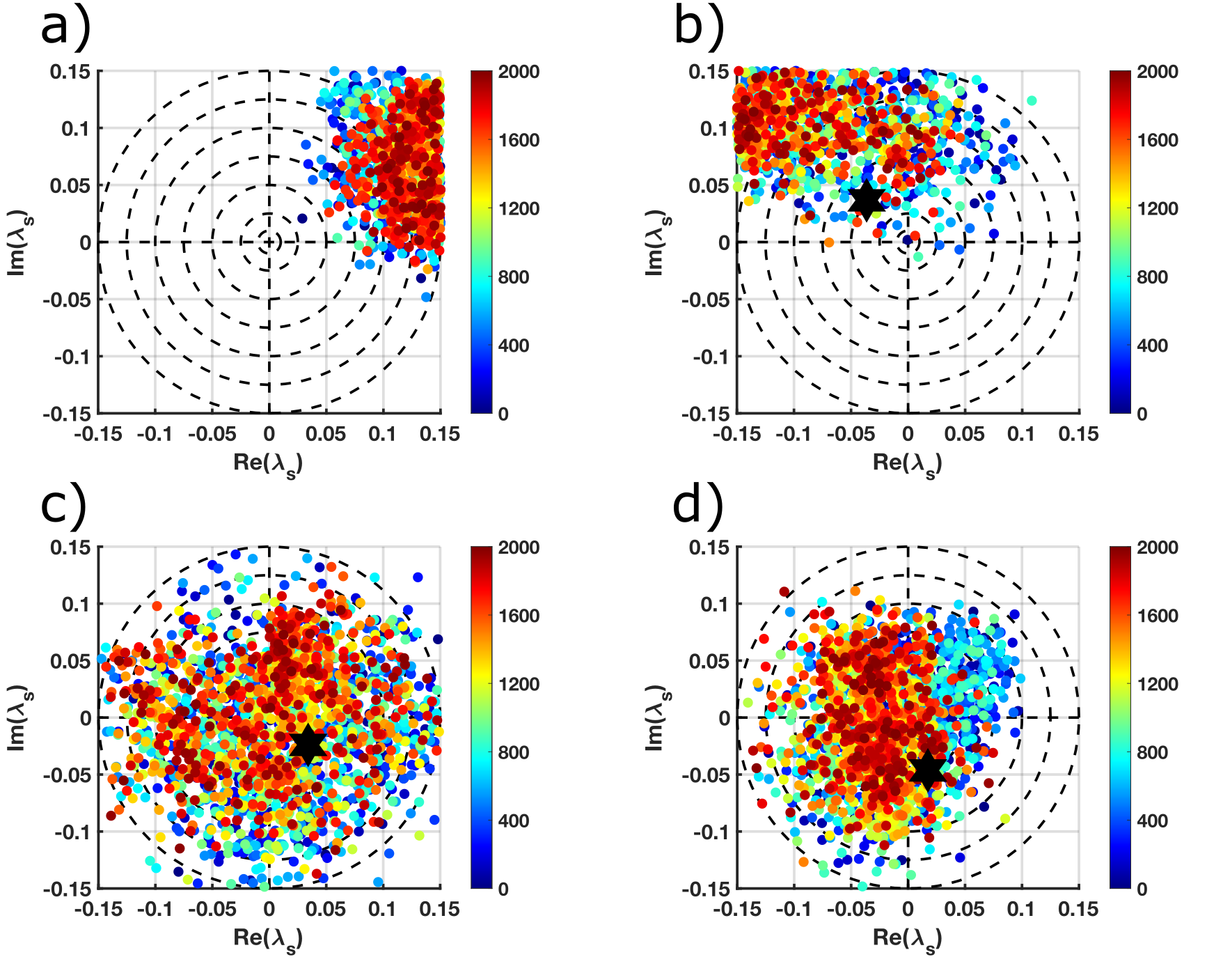
Figure 5: Point clouds of selected $S$-matrix eigenvalues for a random distribution of 2000 metasurface commands. Panels show the point clouds of the smaller eigenvalues of the 2000 scattering matrices at 4 selected frequencies. The colored circles are the $S$-matrix eigenvalues, and are color coded by the specific command, from 1 to 2000. The large black hexagrams indicate the position of the eigenvalue of $S_{\text{rad}}$. a) Candidate at $f$ = 3.0055 GHz, minimum $|\lambda_{s}|$ = $6\times 10^{-2}$. b) Candidate at $f$ = 3.4021 GHz, minimum $|\lambda_{s}|$ = $2\times 10^{-3}$. c) Candidate at $f$ = 3.6564 GHz, minimum $|\lambda_{s}|$ = $5\times 10^{-3}$. d) Candidate at $f$ = 3.9991 GHz, minimum $|\lambda_{s}|$ = $5\times 10^{-4}$.

An open question is how small do the eigenvalues need to be to realize CPA? This is dependent on the specific application and scattering system, as that determines how accurately the eigenvalues can be measured and maintained. For our experimentation, we set $|\lambda_{s}|\leq 5\times 10^{-3}$ as the upper bound and $|\lambda_{s}|\leq 1\times 10^{-3}$ as the goal for realizing CPA.

We adopt the same basic algorithm used for power minimization but initialize it differently. We apply a random set of commands to the metasurface and then select a candidate eigenvalue with a specified magnitude. Figure 6 presents the results of 27 separate CPA eigenvalue optimization experiments. Fig. 6a shows the behavior of 4 selected cases away from the origin for $|\lambda_{s}|<0.15$, and Fig. 6b shows the behavior at the CPA condition for $|\lambda_{s}|<5\times 10^{-3}$. Only 3 of the 4 selected cases reach the CPA threshold. Fig. 6c presents the collection of all 27 experiments, with the four shown in detail in panels a) and b) color coded. Each case was initialized with an eigenvalue magnitude chosen in the range $0.075\leq|\lambda_{s}|\leq 0.5$. The case that started with $|\lambda_{s}|=0.5$ is enclosed by a triangle, the cases that started with $|\lambda_{s}|=0.2$ are enclosed by squares and the case that started with $|\lambda_{s}|=0.175$ is enclosed by a circle. All the rest started with $|\lambda_{s}|\leq 0.15$. Three cases initialized with $|\lambda_{s}|=0.15$ did not quite make the CPA threshold, $|\lambda_{s}|\leq 5\times 10^{-3}$. Two cases were within a factor of 2, $|\lambda_{s}|\leq 9\times 10^{-3}$, while the third was within $\sim$20%, $|\lambda_{s}|=6\times 10^{-3}$ .

Utilizing the iterative optimization algorithm to change the metasurface, we are able to drive eigenvalues towards the origin in all cases, but the algorithm stalls at different points. The closer we get to the origin, the more difficult it becomes to reduce the eigenvalue further. As with the coldspot optimization, the stochastic nature of the algorithm plays a role in where convergence is reached. The overall performance could be improved by increasing the convergence criteria or making the algorithm adaptive so that it tracks multiple candidates and switches to another candidate when the optimization stalls.

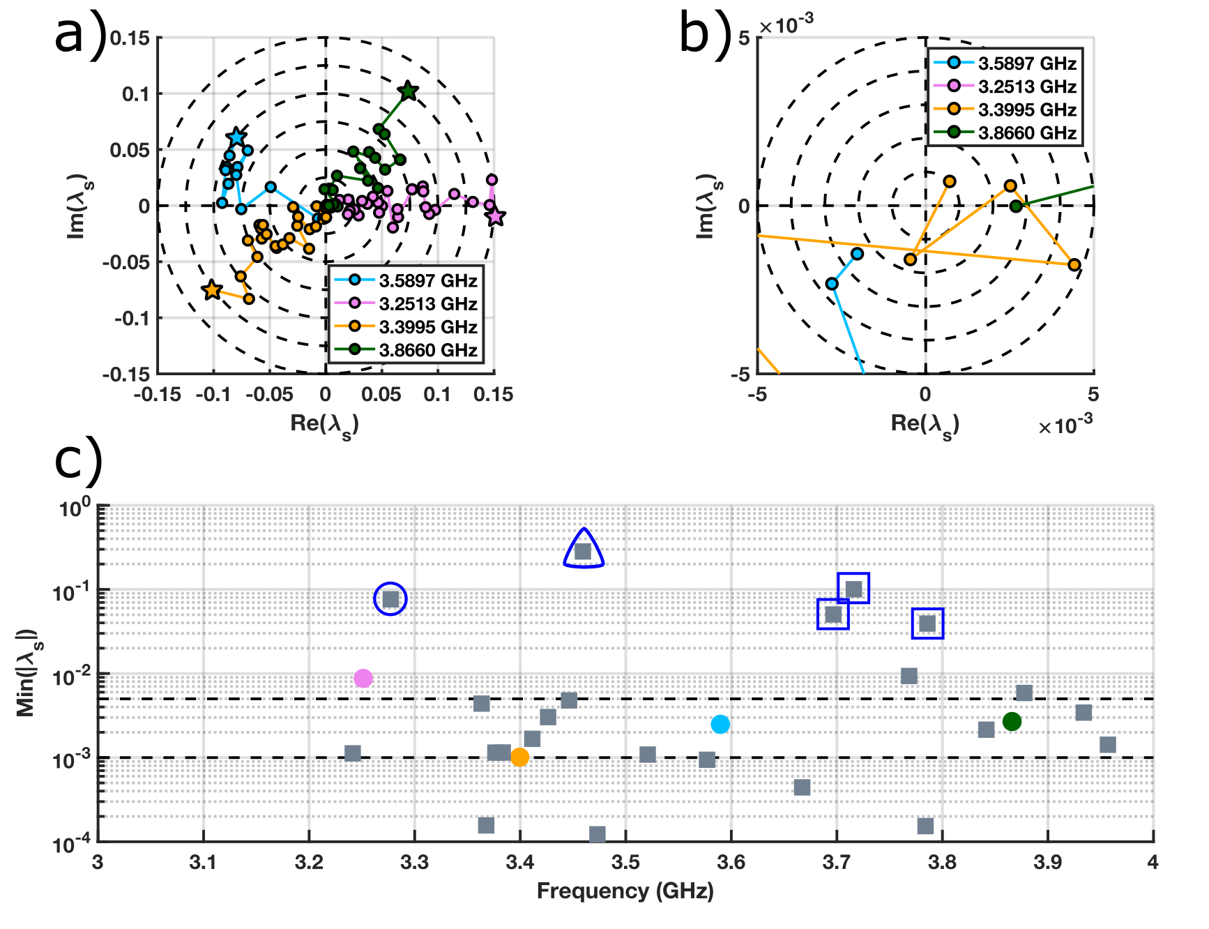
Figure 6: Experimental $S$-matrix eigenvalue trajectories for realization of Coherent Perfect Absorption (CPA) states. a) and b) Directed trajectories for eigenvalues showing the random walk nature of the algorithm and demonstrating mobility of selected eigenvalue candidates. a) Zoomed out view showing selection of initial $S$-matrix eigenvalue candidates and behavior away from the origin, the bulls-eye circles are spaced at radii incrementing by $2.5\times 10^{-2}$. The starting eigenvalue magnitude in each case is identified by a star. b) Close up view showing behavior near the origin, the bulls-eye circles are spaced at radii incrementing by $1\times 10^{-3}$. Of the four cases shown, only 3 were able to get inside the inner rings near the origin where $|\lambda_{s}|<5\times 10^{-3}$. c) Minimum achieved eigenvalue magnitude for each performed experiment. The circles indicate data that is shown in the upper plots and are color coded to match. The gray squares indicate an experiment that was performed but whose detailed trajectory is not shown in the upper plots. The dashed black lines indicate the cross over points of $5\times 10^{-3}$ and $1\times 10^{-3}$. The enclosed squares indicate cases where the initial eigenvalue magnitude $|\lambda_{s}|>$ 0.15. $|\lambda_{s}|$ = 0.5 for the triangle, $|\lambda_{s}|$ = 0.2 for the squares, and $|\lambda_{s}|$ = 0.175 for the circle.

As a final step, we want to verify that the CPA state has been achieved. Because the CPA state is found by minimizing the eigenvalues of the scattering matrix, verification requires that we apply the corresponding $S$-matrix eigenvector. This can be done using a network analyzer with 2 independent sources and an external phase shifter [27]. After directing a particular eigenvalue towards the origin, the network analyzer was configured for independent source operation and the amplitude and phase were adjusted to generate the eigenvector, as described in the supplemental material. The presence of a CPA state is verified by looking at the ratio of all the power emerging from the cavity to all the power injected into the cavity, $P_{\text{out}}/P_{\text{in}}$. Sensitivity to changes in the eigenvector can be determined by making small deviations in the relative phase shift or amplitude between the two sources. Sensitivity to the eigenvalue can be determined by small changes in frequency.

A set of parameter sweeps that verify a CPA state was realized are presented in Figure 7. Fig. 7e shows the $S$-matrix eigenvalue magnitude trajectory during optimization prior to performing the verification sweeps. The overall experimental setup is shown in Fig. 7f, which shows that a 2-source network analyzer was configured with independent source operation and connected to the cavity with an external phase shifter on port 1. This allows us to produce the appropriate eigenvector by controlling the relative amplitude with the network analyzer and the relative phase with the phase shifter. The metric for the sweeps is the power ratio, $P_{\text{out}}/P_{\text{in}}$, of all the power emerging from the cavity to all the power injected into the cavity. At the CPA condition, all the energy should be absorbed. However, due to instrumentation limitations with the system noise floor, the smallest measurable power ratio is $\sim$10^-6. Before performing the sweeps, the eigenvector was tweaked to provide the closest CPA state realization and then the parameters were varied to determine the sensitivity of the power ratio.

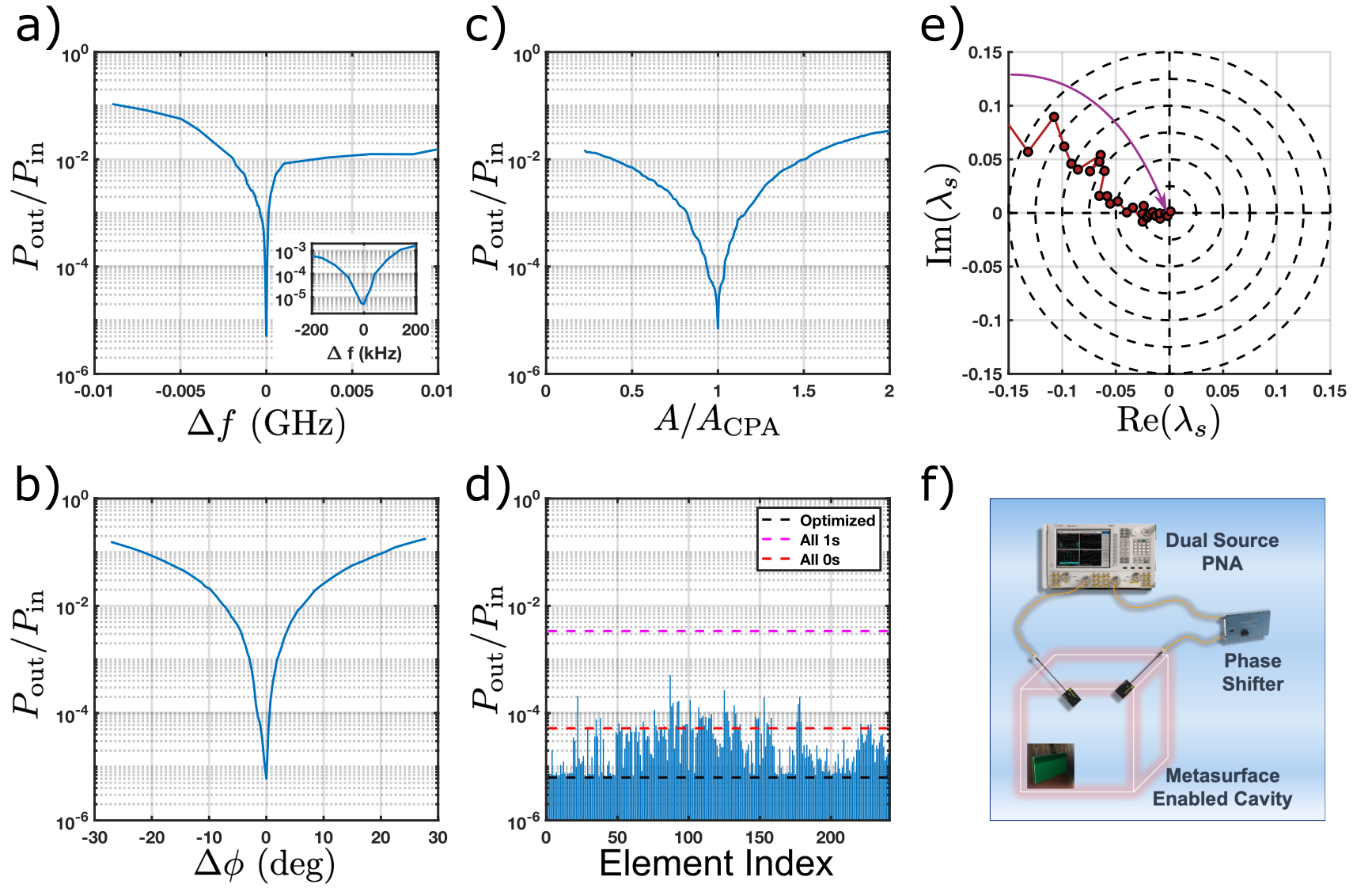
Figure 7: Coherent Perfect Absorption (CPA) state verification at 3.6697 GHz. a) Frequency sweep showing the power ratio, $P_{\text{out}}/P_{\text{in}},$ over a $\pm$ 10 MHz window, with the inset providing a closeup of the null in a $\pm$ 200 kHz window. b) $P_{\text{out}}/P_{\text{in}}$ vs. phase difference, $\Delta\phi$, showing the power ratio over a $\pm$ 30^∘ window. c) $P_{\text{out}}/P_{\text{in}}$ vs. relative amplitude showing the power ratio when driving port 1 with an amplitude $\sim$0-2 times the CPA amplitude ($\text{A}_{\text{CPA}}$). d) Metasurface command sweep showing the power ratio when toggling individual elements relative to the optimized set. Each bar indicates the power ratio when that particular element was flipped between a 1 or a 0. The black dashed line shows the power ratio for the optimized state, the red dashed line shows the power ratio for the all 0s state, and the magenta dashed line shows the power ratio for the all 1s state. e) Eigenvalue magnitude trajectory during optimization of the CPA state prior to performing the verification sweeps. Minimum achieved $|\lambda_{s}|=4\times 10^{-4}$. f) Diagram showing experimental setup for applying CPA eigenvector excitation and verification sweeps.

Fig. 7a shows the results of the frequency sweep performed in a $\pm$ 10 MHz window around 3.6697 GHz, with the inset showing a closeup in a $\pm$ 200 kHz window. The width of the deep null is $\sim$200 kHz, which matches the null widths found during cold spot generation. Fig. 7b shows the results of the phase sweep, which was performed by adjusting the external phase shifter. Here, $\Delta\phi$ represents the phase shift at port 1 away from the CPA eigenvector phase. Fig. 7c shows the results of the relative amplitude sweep. This was performed by sweeping the power injected into port 1 from -10 dBm to +10 dBm. The $x$-axis is then scaled to show the relative change in injected amplitude from the initial CPA state. In each of these cases, the minimium power ratio is $\sim 6\times 10^{-6}$ and shows a steep cusp-like increase with the various parameters. Fig. 7d shows the results of the metasurface command sweep. In this case, the 240 individual metasurface elements were toggled to determine the impact of a single element on the CPA state. Several elements had negligible impact on the power ratio in comparison with the optimized value as seen in the dashed black line, but no toggles were found with clearly better performance. The elements in the center of the metasurface have a stronger impact than those at the edges of the metasurface, but the largest change from the CPA condition was observed by setting all the elements to 1s as shown in the dashed magenta line.

V Conclusions

We have demonstrated the ability of a programmable metasurface to generate microwave coldspots in a chaotic cavity at arbitrary frequencies and showed this capability exists even when applied over multiple frequency bands simultaneously. The coldspots can be generated for different bandwidths and mulitple input port configurations that induce additional angular and spatial diversity. We have also utilized the programmable metasurface to control the eigenvalues of the scattering matrix and direct them towards the origin to realize a CPA state for the cavity. Finally, we verified the existence of a CPA state and demonstrated the sensitivity to parameter sweeps in frequency, phase, amplitude, and metasurface configuration. All of this is accomplished with a metasurface that covers only 1.5% of the interior surface area of the cavity and a unique and effective stochastic algorithm to find desired outcomes despite the enormous space of possible metasurface commands.

Future research directions include quantitatively analyzing CPA in the framework of the Random Coupling Model [49, 6, 30, 32], and using deep learning to facilitate generating optimal metasurface commands to minimize power and/or realize CPA states.

VI Acknowledgements

We thank Joseph Miragliotta, David Shrekenhamer, and Robert Schmidt for providing the metasurface and supporting detailed discussions on operational use. We also thank Tsampikos Kottos for insights into CPA, and Lei Chen for instructions on performing the various CPA verification sweeps. Funding for this work was provided through AFOSR COE Grant FA9550-15-1-0171 and ONR Grant N000141912481.

VII Author Contributions

B. Frazier performed the experiments and processed the data under the supervision of T. M. Antonsen and S. M. Anlage. B. Frazier prepared the manuscript with input from all co-authors.

VIII Competing Interests

The authors declare no competing interests.

IX Materials and Correspondence

Correspondence and requests for materials should be addressed to B. Frazier (email: benjamin.frazier@jhuapl.edu).

X Data Availability

The data and analysis scripts that support results presented within this paper and other findings of this study are available from the corresponding author upon reasonable request.

References

- Leach and Alexander [1995] R. D. Leach and M. B. Alexander, Electronic systems failures and anomalies attributed to electromagnetic interference, Tech. Rep. NASA-RP-1374 (NASA, 1995).
- Hemmady et al. [2012] S. Hemmady, T. M. Antonsen, E. Ott, and S. M. Anlage, Statistical Prediction and Measurement of Induced Voltages on Components Within Complicated Enclosures: A Wave-Chaotic Approach, IEEE Transactions on Electromagnetic Compatibility 54, 758 (2012).
- Berry [1977] M. V. Berry, Regular and irregular semiclassical wavefunctions, Journal of Physics A: Mathematical and General 10, 2083– (1977).
- Haake [2010] F. Haake, Quantum Signatures of Chaos (Springer, Berlin, Heidelberg, 2010).
- Ott [2002] E. Ott, Chaos in dynamical systems, 2nd ed. (Cambridge University Press, Cambridge, U.K. ; New York, 2002).
- Zheng et al. [2006a] X. Zheng, T. M. Antonsen, and E. Ott, Statistics of Impedance and Scattering Matrices in Chaotic Microwave Cavities: Single Channel Case, Electromagnetics 26, 3 (2006a).
- Epstein et al. [2015] A. Epstein, J. P. S. Wong, and G. V. Eleftheriades, Design and applications of Huygens metasurfaces, in 2015 9th International Congress on Advanced Electromagnetic Materials in Microwaves and Optics (METAMATERIALS) (2015) pp. 67–69.
- Chen et al. [2018] M. Chen, M. Kim, A. M. Wong, and G. V. Eleftheriades, Huygens’ metasurfaces from microwaves to optics: a review, Nanophotonics 7, 1207 (2018).
- He et al. [2019] Q. He, S. Sun, and L. Zhou, Tunable/Reconfigurable Metasurfaces: Physics and Applications, Research 2019, 1 (2019).
- Vellekoop and Mosk [2007] I. M. Vellekoop and A. P. Mosk, Focusing coherent light through opaque strongly scattering media, Optics Letters 32, 2309 (2007).
- Li et al. [2017a] L. Li, T. Jun Cui, W. Ji, S. Liu, J. Ding, X. Wan, Y. Bo Li, M. Jiang, C.-W. Qiu, and S. Zhang, Electromagnetic reprogrammable coding-metasurface holograms, Nature Communications 8, 197 (2017a).
- Sabino et al. [2017] J. Sabino, G. Figueira, and P. André, Wavefront spatial-phase modulation in visible optical communications, Microwave and Optical Technology Letters 59, 1538 (2017).
- Li and Wang [2017] S. Li and J. Wang, Adaptive free-space optical communications through turbulence using self-healing Bessel beams, Scientific Reports 7, 43233 (2017).
- Ameri et al. [2019] E. Ameri, S. H. Esmaeli, and S. H. Sedighy, Ultra Wideband Radar Cross Section Reduction by Using Polarization Conversion Metasurfaces, Scientific Reports 9, 478 (2019).
- Tang et al. [2019] W. Tang, J. Y. Dai, M. Chen, X. Li, Q. Cheng, S. Jin, K.-K. Wong, and T. J. Cui, Programmable metasurface-based RF chain-free 8PSK wireless transmitter, Electronics Letters 55, 417 (2019).
- Imani et al. [2020] M. F. Imani, J. N. Gollub, O. Yurduseven, A. V. Diebold, M. Boyarsky, T. Fromenteze, L. Pulido-Mancera, T. Sleasman, and D. R. Smith, Review of Metasurface Antennas for Computational Microwave Imaging, IEEE Transactions on Antennas and Propagation 68, 1860 (2020).
- Lemoult et al. [2009] F. Lemoult, G. Lerosey, J. de Rosny, and M. Fink, Manipulating Spatiotemporal Degrees of Freedom of Waves in Random Media, Physical Review Letters 103, 173902 (2009).
- Kamali et al. [2017] S. M. Kamali, E. Arbabi, A. Arbabi, Y. Horie, M. Faraji-Dana, and A. Faraon, Angle-Multiplexed Metasurfaces: Encoding Independent Wavefronts in a Single Metasurface under Different Illumination Angles, Physical Review X 7, 041056 (2017).
- del Hougne et al. [2020] P. del Hougne, M. Davy, and U. Kuhl, Optimal Multiplexing of Spatially Encoded Information across Custom-Tailored Configurations of a Metasurface-Tunable Chaotic Cavity, Physical Review Applied 13, 041004 (2020).
- Gros et al. [2020] J.-B. Gros, P. del Hougne, and G. Lerosey, Tuning a regular cavity to wave chaos with metasurface-reconfigurable walls, Physical Review A 101, 061801 (2020).
- Dupré et al. [2015] M. Dupré, P. del Hougne, M. Fink, F. Lemoult, and G. Lerosey, Wave-Field Shaping in Cavities: Waves Trapped in a Box with Controllable Boundaries, Physical Review Letters 115, 017701 (2015).
- del Hougne et al. [2016a] P. del Hougne, F. Lemoult, M. Fink, and G. Lerosey, Spatiotemporal Wave Front Shaping in a Microwave Cavity, Physical Review Letters 117, 134302 (2016a).
- Jang et al. [2018] M. Jang, Y. Horie, A. Shibukawa, J. Brake, Y. Liu, S. M. Kamali, A. Arbabi, H. Ruan, A. Faraon, and C. Yang, Wavefront shaping with disorder-engineered metasurfaces, Nature Photonics 12, 84 (2018).
- Zhao et al. [2020] H. Zhao, Y. Shuang, M. Wei, T. J. Cui, P. d. Hougne, and L. Li, Metasurface-assisted massive backscatter wireless communication with commodity Wi-Fi signals, Nature Communications 11, 3926 (2020).
- Chong et al. [2010] Y. D. Chong, L. Ge, H. Cao, and A. D. Stone, Coherent Perfect Absorbers: Time-Reversed Lasers, Physical Review Letters 105, 053901 (2010).
- Pichler et al. [2019] K. Pichler, M. Kühmayer, J. Böhm, A. Brandstötter, P. Ambichl, U. Kuhl, and S. Rotter, Random anti-lasing through coherent perfect absorption in a disordered medium, Nature 567, 351 (2019).
- Chen et al. [2020] L. Chen, T. Kottos, and S. M. Anlage, Perfect Absorption in Complex Scattering Systems with or without Hidden Symmetries, arXiv:2001.00956 (2020).
- Schmid et al. [2020] R. L. Schmid, D. B. Shrekenhamer, O. F. Somerlock, A. C. Malone, T. A. Sleasman, and R. S. Awadallah, S-band GaAs FET Reconfigurable Reflectarray for Passive Communications, in 2020 IEEE Radio and Wireless Symposium (RWS) (IEEE, San Antonio, TX, USA, 2020) pp. 91–93.
- Addissie et al. [2019] B. Addissie, J. Rodgers, and T. Antonsen, Extraction of the coupling impedance in overmoded cavities, Wave Motion 87, 123 (2019).
- Hemmady et al. [2005a] S. Hemmady, X. Zheng, E. Ott, T. M. Antonsen, and S. M. Anlage, Universal Impedance Fluctuations in Wave Chaotic Systems, Physical Review Letters 94, 014102 (2005a).
- Yeh et al. [2010a] J.-H. Yeh, J. A. Hart, E. Bradshaw, T. M. Antonsen, E. Ott, and S. M. Anlage, Universal and nonuniversal properties of wave-chaotic scattering systems, Physical Review E 81, 025201 (2010a).
- Gradoni et al. [2014] G. Gradoni, J.-H. Yeh, B. Xiao, T. M. Antonsen, S. M. Anlage, and E. Ott, Predicting the statistics of wave transport through chaotic cavities by the random coupling model: A review and recent progress, Wave Motion 51, 606 (2014).
- Kaina et al. [2015] N. Kaina, M. Dupré, G. Lerosey, and M. Fink, Shaping complex microwave fields in reverberating media with binary tunable metasurfaces, Scientific Reports 4, 6693 (2015).
- Popoff et al. [2010] S. M. Popoff, G. Lerosey, R. Carminati, M. Fink, A. C. Boccara, and S. Gigan, Measuring the Transmission Matrix in Optics: An Approach to the Study and Control of Light Propagation in Disordered Media, Physical Review Letters 104, 100601 (2010).
- Drémeau et al. [2015] A. Drémeau, A. Liutkus, D. Martina, O. Katz, C. Schülke, F. Krzakala, S. Gigan, and L. Daudet, Reference-less measurement of the transmission matrix of a highly scattering material using a DMD and phase retrieval techniques, Optics Express 23, 11898 (2015).
- del Hougne et al. [2016b] P. del Hougne, B. Rajaei, L. Daudet, and G. Lerosey, Intensity-only measurement of partially uncontrollable transmission matrix: demonstration with wave-field shaping in a microwave cavity, Optics Express 24, 18631 (2016b).
- Watts et al. [2014] C. M. Watts, D. Shrekenhamer, J. Montoya, G. Lipworth, J. Hunt, T. Sleasman, S. Krishna, D. R. Smith, and W. J. Padilla, Terahertz compressive imaging with metamaterial spatial light modulators, Nature Photonics 8, 605 (2014).
- Watts et al. [2016] C. M. Watts, C. C. Nadell, J. Montoya, S. Krishna, and W. J. Padilla, Frequency-division-multiplexed single-pixel imaging with metamaterials, Optica 3, 133 (2016).
- Dorrer and Qiao [2018] C. Dorrer and J. Qiao, Direct binary search for improved coherent beam shaping and optical differentiation wavefront sensing, Applied Optics 57, 8557 (2018).
- [40] Hackrf one, https://greatscottgadgets.com/hackrf/one/.
- [41] Bladerf, https://www.nuand.com/bladerf-1/.
- Kottos and Smilansky [1997] T. Kottos and U. Smilansky, Quantum Chaos on Graphs, Physical Review Letters 79, 4794 (1997).
- Kottos and Smilansky [2000] T. Kottos and U. Smilansky, Chaotic Scattering on Graphs, Physical Review Letters 85, 968 (2000).
- Fyodorov et al. [2017] Y. V. Fyodorov, S. Suwunnarat, and T. Kottos, Distribution of zeros of the S -matrix of chaotic cavities with localized losses and coherent perfect absorption: non-perturbative results, Journal of Physics A: Mathematical and Theoretical 50, 30LT01 (2017).
- Li et al. [2017b] H. Li, S. Suwunnarat, R. Fleischmann, H. Schanz, and T. Kottos, Random Matrix Theory Approach to Chaotic Coherent Perfect Absorbers, Physical Review Letters 118, 044101 (2017b).
- F. Imani et al. [2020] M. F. Imani, D. R. Smith, and P. del Hougne, Perfect absorption in a disordered medium with programmable meta-atom inclusions, Advanced Functional Materials , 2005310 (2020).
- Asadchy et al. [2015] V. Asadchy, I. Faniayeu, Y. Ra’di, S. Khakhomov, I. Semchenko, and S. Tretyakov, Broadband Reflectionless Metasheets: Frequency-Selective Transmission and Perfect Absorption, Physical Review X 5, 031005 (2015).
- Krasnok et al. [2018] A. Krasnok, D. G. Baranov, A. Generalov, S. Li, and A. Alù, Coherently enhanced wireless power transfer, Phys. Rev. Lett. 120, 143901 (2018).
- Zheng et al. [2006b] X. Zheng, T. M. Antonsen, and E. Ott, Statistics of Impedance and Scattering Matrices of Chaotic Microwave Cavities with Multiple Ports, Electromagnetics 26, 37 (2006b).
- Hemmady et al. [2006] S. Hemmady, X. Zheng, J. Hart, T. M. Antonsen, E. Ott, and S. M. Anlage, Universal properties of two-port scattering, impedance, and admittance matrices of wave-chaotic systems, Physical Review E 74, 036213 (2006).
- Yeh [2013] J.-H. Yeh, Wave Chaotic Experiments and Models for Complicated Wave Scattering Systems, Ph.D. thesis, University of Maryland (2013).
- Yeh et al. [2012] J.-H. Yeh, T. M. Antonsen, E. Ott, and S. M. Anlage, First-principles model of time-dependent variations in transmission through a fluctuating scattering environment, Physical Review E 85, 015202 (2012).
- Hart et al. [2009] J. A. Hart, T. M. Antonsen, and E. Ott, Effect of short ray trajectories on the scattering statistics of wave chaotic systems, Physical Review E 80, 041109 (2009).
- Yeh et al. [2010b] J.-H. Yeh, J. A. Hart, E. Bradshaw, T. M. Antonsen, E. Ott, and S. M. Anlage, Experimental examination of the effect of short ray trajectories in two-port wave-chaotic scattering systems, Physical Review E 82, 041114 (2010b).
- Hemmady et al. [2005b] S. Hemmady, X. Zheng, T. M. Antonsen, E. Ott, and S. M. Anlage, Universal statistics of the scattering coefficient of chaotic microwave cavities, Physical Review E 71, 056215 (2005b).