Quantum State Complexity in Computationally Tractable Quantum Circuits

Abstract

Characterizing the quantum complexity of local random quantum circuits is a very deep problem with implications to the seemingly disparate fields of quantum information theory, quantum many-body physics and high energy physics. While our theoretical understanding of these systems has progressed in recent years, numerical approaches for studying these models remains severely limited. In this paper, we discuss a special class of numerically tractable quantum circuits, known as quantum automaton circuits, which may be particularly well suited for this task. These are circuits which preserve the computational basis, yet can produce highly entangled output wave functions. Using ideas from quantum complexity theory, especially those concerning unitary designs, we argue that automaton wave functions have high quantum state complexity. We look at a wide variety of metrics, including measurements of the output bit-string distribution and characterization of the generalized entanglement properties of the quantum state, and find that automaton wave functions closely approximate the behavior of fully Haar random states. In addition to this, we identify the generalized out-of-time ordered 2k-point correlation functions as a particularly useful probe of complexity in automaton circuits. Using these correlators, we are able to numerically study the growth of complexity well beyond the scrambling time for very large systems. As a result, we are able to present evidence of a linear growth of design complexity in local quantum circuits, consistent with conjectures from quantum information theory.

I Introduction

Understanding the evolution of a quantum wave functions from a simple initial state to a generic vector in an exponentially large Hilbert space is a notoriously difficult problem in modern theoretical physics. Aspects of this evolution underlie important open problems in quantum information theory, quantum many-body physics and high energy physics. Great progress has been made in recent years by focusing on local random circuit models, which provide a relatively clean system where these dynamics can be studied Nahum et al. (2017, 2018, 2018); Khemani et al. (2018); von Keyserlingk et al. (2018). A particularly important element of a generic quantum dynamics is the concept of information scrambling. Originally studied in the context of black holes Hayden and Preskill (2007); Page (1993), scrambling defines the process whereby initially local information spreads throughout the system and becomes stored in the many-body non-local entanglement of the state. Similar works have since used this concept to gain insight into how closed quantum systems reach equilibrium and thermalize under a generic Hamiltonian dynamics Nandkishore and Huse (2015).

Two of the main tools which have been used to understand information scrambling are the entanglement entropy of the quantum state and the evolution of the out-of-time-ordered (OTO) correlation function. It can be shown that the entanglement entropy in these systems grows linearly with time until it reaches a near maximal value Nahum et al. (2017), and a decay of the out-of-time ordered 4-point correlator has been shown to be equivalent to the Hayden-Preskill definition of scrambling Hosur et al. (2016). While such measurements are useful, it has become clear that these relatively simple measures cannot capture all the fine grained aspects of the random unitary evolution. Two states may look maximally scrambled according to these two measures and yet have important differences in the precise way the information is stored non-locally.

Quantum state complexity theory has been suggested as a means to quantify these differences Brandão et al. (2019); Roberts and Yoshida (2017); Liu et al. (2018a). Roughly speaking, the complexity of a quantum state is the depth of the smallest local unitary circuit which can create the state from an initial product state. In random circuit models, the growth of quantum state complexity directly corresponds to an increased difficulty in distinguishing the pure quantum state from the maximally mixed state Brandão et al. (2019). This is a physical property whereby initially local information is more effectively hidden in high complexity states.

It is known that a generic Haar random state will have a complexity which is exponentially large in system size $N$. As a result, almost all quantum states cannot be efficiently simulated, even with a quantum computer Poulin et al. (2011). A state which is the output of a depth $D$ random circuit composed from a universal gate set will have a complexity which is conjectured to grow linearly with $D$ Brown and Susskind (2018); Susskind (2018). Ensembles of these wave functions form what is known as an approximate projective unitary k-design Gross et al. (2007). Measurements on k-designs can approximate, for large enough k, arbitrarily high moments of measurements on fully Haar random states. On the other hand, states which are output from Clifford circuits in general form only a unitary 2-design Zhu et al. (2016). Although these wave functions display volume law entanglement and information scrambling, they are still of relatively low complexity and only approximate a few moments of the Haar random states.

In this paper, we show that high complexity quantum states can be prepared from a special type of non-universal local quantum circuit. These circuits, which we call ‘automaton’ quantum circuits, consist of any quantum gate which preserves the computational basis. These automaton circuits have very recently started to be used as a tool for studying dynamics in quantum systems Gopalakrishnan and Zakirov (2018); Gopalakrishnan (2018); Iaconis et al. (2019). Specifically, in Iaconis et al. (2019), it was realized that the operator entanglement and OTOC properties of such circuits appear to give results which are identical to that of a generic chaotic dynamics. We go beyond this and show that, when acting on initial product states not in the computational basis, automaton circuits produce highly entangled wave functions in which the quantum state complexity grows with circuit depth in the same way as in universal local random circuits. Furthermore, the evolution of these wave functions can be efficiently simulated classically using a quantum Monte Carlo algorithm which we describe. This may be appreciated in the context of several other results in quantum information theory which demonstrate that the presence of entanglement in a quantum state is not enough to show that a quantum algorithm which simulates the state achieves a speedup over a classical algorithm Gottesman (1998); Aaronson and Gottesman (2004); Van den Nest (2013). Our results imply that complexity of the wave function is also not a sufficient condition for such purposes.

We do not attempt to provide a rigorous proof that automaton circuits output states of high complexity. Instead, we characterize the complexity of the automaton states using a series of measurements which were developed to probe the fine-detailed structure of wave functions. We consider metrics such as the generalized $k^{\text{th}}$ Renyi entropy Liu et al. (2018a, b) and the sampled output bit-string distribution Brandão et al. (2016), which can be used to differentiate between high and low complexity states which both have near maximal bipartite entanglement entropy. We also consider other measurements such as the fluctuation of entanglement entropy and the level spacing distribution of the entanglement spectrum. We will see that by these measures, the automaton wave functions behave like highly complex states.

In a dynamical context, the generalized k-point OTO correlation functions can describe the growth of quantum state complexity beyond the scrambling time Roberts and Yoshida (2017). Again, according to this metric, complexity in automaton circuits appears to grow in the same way as in generic Haar random circuits. Further, using our efficient quantum Monte Carlo algorithm, we are able to numerically study the growth of these OTO correlation functions in this poorly understood “beyond scrambling regime” for very large circuits. By doing this, we are able to identify specific k-point OTO correlation functions which appear to track the precise rate of complexity growth in local random circuits and give results which are consistent with the linear growth conjectured in the literature Brown and Susskind (2018); Brandão et al. (2019).

The rest of this paper is organized as follows. In section II, we will introduce and describe key properties of the quantum automaton circuits. We also describe the quantum Monte Carlo algorithm we use to simulate these wave functions. In section III, we review the concept of quantum state complexity, and describe several measurements which we use to distinguish between high and low complexity states. We will see that by these metrics, automaton states behave like high complexity Haar random states. We contrast these results to those of low complexity Clifford wave functions. In section IV, we discuss the generalized k-point out-of-time-ordered correlator as a probe of complexity growth in dynamic systems. We will see that automaton circuits can make use of these correlation functions to give us new insights into complexity growth beyond scrambling in local quantum circuits. In section V we summarize our results and discuss potential applications of this work.

II Automaton Quantum Circuits

II.1 Definitions and Review of Previous Results

In this paper, we define automaton dynamics simply as any unitary evolution of a quantum system which does not generate any entanglement when applied to product states in an appropriate basis (which we will choose to be the computational basis). As stated in Iaconis et al. (2019), an automaton unitary operator $U$ acting on an appropriate set of product states in a $d$-dimensional Hilbert space - labeled $|m\rangle$, with $m\in\{0,\dots,d-1\}$ - permutes these states up to a phase factor, i.e.

$$U|m\rangle=e^{i\theta_{m}}|\pi(m)\rangle\,$$ (1)

where $\pi\in S_{d}$ is an element of the permutation group on $d$ elements.

Similar unitary circuits with sparse output distributions have been studied in the quantum information literature, where it was shown that efficient classical simulation methods exist Van Den Nest (2011); Schwarz and den Nest (2013). These circuits were first studied in a condensed matter context in integrable models in Gopalakrishnan and Zakirov (2018) and Gopalakrishnan (2018). In Iaconis et al. (2019), it was realized that a generic automaton evolution leads to dynamics which appear to show ‘quantum chaotic’ behavior. The out-of-time ordered correlators propagate ballistically and saturate to the consistent values for a Haar scrambled operator. While automaton circuits do not generate entanglement in the computational basis, a key property is that they do generically generate a high degree of operator entanglement. That is, the evolution

$$\mathcal{O}\rightarrow U^{\dagger}\mathcal{O}U$$ (2)

can be very complex and shows many of the generic features of a Haar random unitary evolution.

One important example of such an automaton gate is a quantum version of the CCNOT gate

$$CCNOT(\theta)_{123}=1-\Pi_{12}-\Pi_{12}e^{i\theta}X_{3}.$$ (3)

When $\theta=0$, this is the classical Toffoli gate which is known to be universal for classical reversible computation and can therefore implement any permutation $\pi\in S_{d}$ on the computational basis states $|m\rangle$, $m\in\{0,\dots d-1\}$. When $\theta\neq 0$, such a gate also includes a state dependent phase.

A second important automaton gate set is the set

$$\{\,\text{CNOT},\text{SWAP},R_{z}(\theta)\,\},$$ (4)

where $R_{z}(\theta)=e^{i\theta Z}$ implements a single qubit rotation about the Z axis. At $\theta=\pi/2$, all three gates belong to the Clifford group. The set of Clifford gates is capable of generating volume law entanglement when applied to an appropriate initial product state, and the dynamics can be exactly simulated classically Gottesman (1998); Aaronson and Gottesman (2004). Therefore, the automaton gate set generalizes the above Clifford group by allowing single qubit rotations by arbitrary angles.

Note that both sets of gates defined above are universal for quantum computation if supplemented by any single qubit gate which does not preserve the computational basis Shi (2002).

We first review a few important analytic results derived in Iaconis et al. (2019), in the case that the automaton circuit is composed of $CCNOT(\theta=0)$. First, an initially local diagonal operator $\mathcal{O}_{diag}$, will evolve into a superposition over $O(d)$ other diagonal operators (where $d=2^{N}$ for qubits) and will have a near maximal average operator entanglement. Second, initially off-diagonal operators will evolve into all elements of the conjugacy class of $S_{d}$, which implies that an initial operator can evolve into $O(d^{d})$ possible off-diagonal operators. That is, a generic operator can evolve, under automaton dynamics, into a super-exponential number of other possible operators. Finally, the recurrence time of a quantum evolution describes the time it takes for an initial wave function to return to a nearby quantum state so that $\langle\psi_{0}|U|\psi_{0}\rangle\sim O(1)$. For automaton circuits, the recurrence time of an initial state (not necessarily a product state in the computation basis) corresponds to the order of a random element of the permutation group $S_{d}$ and on average gives $t_{rec}\rightarrow exp(\lambda\sqrt{d/\log(d)})$ as $d\rightarrow\infty$.

We also note that in Iaconis et al. (2019) it was found that the operator spreading in automaton circuits, as quantified by the 4-point out-of-time-ordered correlation function, behaves identically to that of a Haar random chaotic circuit. In particular, the operator weights spreads ballistically with a wave front which broadens with a power law which is consistent with the universal exponents of a generic local chaotic dynamics Nahum et al. (2018).

In what follows, we take a complementary approach and study the evolution of quantum states which are initially product states in a basis orthogonal to the computational basis. We will refer to the output of such circuits as automaton wave functions. This approach allows us to focus on the entanglement and complexity of the resulting wave function, and lets us compare our algorithm with known variational Monte Carlo techniques.

II.2 A Variational Monte Carlo Algorithm

The defining feature of automaton circuits, that computational basis states only evolve to other computational basis states, is what allows us to simulate automaton wave functions on a classical computer. Despite their apparent simplicity, such an evolution produces highly nontrivial wave functions when applied to initial wave functions which are not product states in the computational basis.

We start with an initial ansatz wave function

$$|\psi_{0}\rangle=\sum_{m}c_{m}|m\rangle,$$ (5)

where we assume we know the coefficients $c_{m}$ exactly. Throughout this paper, we will often choose $|\psi_{0}\rangle$ to be a product state in the $X$ basis, $c_{m}=(-1)^{{\bf m}\cdot\bm{\sigma}}/d$, where ${\bf m}$ is a binary vector representation of the integer $m$, and $\bf{\sigma}$ is a vector of Pauli $X_{i}$ eigenvalues of $|\psi_{0}\rangle$. However, this need not be the case, and we can choose any initial state $|\psi_{0}\rangle$ for which we have a variational ansatz $c_{m}$.

We then time evolve the wave function by applying the quantum circuit

$$U_{{\bm{\lambda}}}=\prod_{t=1}^{T}\left[\left(\prod_{j}U_{j,j+1}^{(t)}\right)\left(\prod_{j}U_{j+1,j+2}^{(t)}\right)\right]$$ (6)

where ${\bm{\lambda}}$ are the variational parameters which represent the precise set of gates $\{U_{j,j+1}^{t}\}$ which are applied. The resulting wave function is then

$$|\psi(t)\rangle=U_{\bm{\lambda}}|\psi_{0}\rangle=\sum_{m}c_{m}e^{i\theta_{m}}|\pi_{\bm{\lambda}}(m)\rangle.$$ (7)

Again $\pi_{{\bm{\lambda}}}(m)$, is the permutation on the computational basis states, $|m\rangle$, which is implemented by $U_{\bm{\lambda}}$. Therefore, we can exactly calculate the coefficients of the final wave function $|\psi(t)\rangle=\sum_{x}\psi_{\bm{\lambda}}(x,t)|x\rangle$ as

$$\psi_{\bm{\lambda}}(x,t)=\langle x|\psi(t)\rangle=c_{\pi_{\bm{\lambda}}^{-1}(x)}\exp[i\theta_{\pi_{\bm{\lambda}}^{-1}(x)}].$$ (8)

For a circuit with $N$ qubits and depth $T$, this can be calculated in a time which scales like $O(NT)$. That is, since $|m\rangle$ only evolves to a simple product state, $|\pi(m)\rangle$, instead of a superposition over basis states, we can simply classically sample the initial states $|m\rangle$ and track their time evolution. Nevertheless, as long as $|\psi_{0}\rangle$ is not a product state in the computational basis, $|\psi(t)\rangle$ will generally evolve into a volume law entangled state. In this way we are able to classically simulate the circuit evolution of highly entangled quantum wave functions in a way which is equivalent to the well known variational Monte Carlo methods.

We can therefore efficiently calculate estimates for simple operator expectation values as

$$\langle\mathcal{O}\rangle = \langle\psi_{0}|U^{\dagger}\mathcal{O}U|\psi_{0}\rangle$$ (9)

$$= \sum_{xy}c_{y}^{*}c_{x}^{\phantom{*}}\bigg{\langle}y\bigg{|}\bigg{(}\prod_{t}U_{t}^{\dagger}\bigg{)}\mathcal{O}\bigg{(}\prod_{t}U_{t}\bigg{)}\bigg{|}x\bigg{\rangle}$$

$$= \sum_{x,y}\psi^{*}_{\bm{\lambda}}(\pi(y),t)\psi_{\bm{\lambda}}(\pi(x),t)\,o\big{(}\pi(x),\pi(y)\big{)}.$$ (10)

Since $U$ is an automaton circuit, then if $\mathcal{O}$ is a simple Pauli operator we have $o(\pi(x),\pi(y))=f(\pi(x))\delta(y,x^{\prime})$ with

$$x^{\prime} = \pi_{\bm{\lambda}}^{-1}(\pi_{\mathcal{O}}(\pi_{\bm{\lambda}}(x)).$$ (11)

Therefore, we can write

$$\langle\mathcal{O}\rangle \approx \frac{1}{M}\sum_{x_{i}=1}^{M}\psi^{*}_{\bm{\lambda}}(\pi(x_{i}^{\prime}),t)\psi_{\bm{\lambda}}(\pi(x_{i}),t)\,f(x_{i})$$ (12)

$$= \frac{1}{M}\sum_{x_{i}=1}^{M}c_{x_{i}^{\prime}}^{*}c_{x_{i}}^{\phantom{*}}e^{i\left(\theta_{x_{i^{\phantom{\prime}}}}-\theta_{x_{i}^{\prime}}\right)}\,f(x_{i}).$$ (13)

Note that for a generic off-diagonal operator $\mathcal{O}$, to determine which state $|x^{\prime}(t)\rangle$ has a nonzero overlap with $\mathcal{O}|x(t)\rangle$, we perform the full forward and backward time evolution in Eq. (9) for each time step independently. Estimating the full time dependence of $\mathcal{O}(t)$ therefore takes a time $O(NT^{2})$. On the other hand, if $\mathcal{O}$ is a diagonal operator, then $x^{\prime}=x$ and we can get an estimate for the entire time evolution in a time that scales like $O(NT)$.

We finally note that using this approach to studying quantum circuit dynamics allows us to make use of other tools developed in the context of variational Monte Carlo algorithms. For example, one may incorporate Jastrow factors Sorella (2005), Lanczos steps Becca et al. (2015); Sorella (2001) or other perturbative corrections to the quantum wave function Iaconis et al. (2018). Furthermore, a promising direction for future work may involve applying automaton circuits to RBM or other neural network wave functions. Such models were studied for a subset of automaton gates in Jónsson et al. (2018).

In the rest of this work, we focus on a specific 1D random circuit model consisting of two site gates in alternating layers as shown in Fig. 1. The gates in this circuit are randomly chosen to be either the two site SWAP or CNOT gates or a single site rotation by a random angle $\theta$, $R_{z}(\theta)=e^{i\theta\hat{Z}}$. We also compare the results to those of a random Clifford circuit, where we randomly choose the gates to be either the two site SWAP or CNOT gates or the single site Hadamard gate.

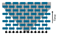
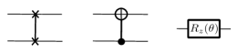
Figure 1: The local random circuit architecture used throughout this paper. Each 2-site gate is chosen randomly to be one of 3 basic automaton gates: the SWAP gate, the CNOT gate or the single site rotation about the z-axis $R_{z}(\theta)=e^{i\theta\hat{Z}}$ (applied independently to each site with a random angle $\theta$).

III Quantum State Complexity

III.1 Background

Quantum complexity theory quantifies the difficulty of particular tasks for a quantum computer, in terms of the minimum number of basic quantum gates a computation requires. Interestingly, in contrast to classical complexity theory, in the quantum setting one can also meaningfully discuss the complexity of a quantum state. Roughly speaking, the complexity of a quantum state is the size of the smallest k-local quantum circuit required to prepare the state from an initial simple reference state. Unlike with classical bit-strings, creating a given quantum state from a given initial state may in general require an exponentially long quantum circuit. In fact, since the number of possible quantum circuits is exponential in gate number, while the number of quantum states is super-exponential in system size, one can show that almost all wave functions require an exponentially long circuit to prepare.

Importantly, the quantum state complexity of a wave function can be directly related to measurable physical properties. This can be seen in the strong notion of complexity put forward in reference Brandão et al. (2019). In their work, the authors define the complexity of a quantum state, $|\psi\rangle$, as the size of the smallest local circuit, $U$, which when combined with measurement, $M$ in the computational basis can distinguish $|\psi\rangle$ from the maximally mixed state $\rho=\frac{1}{d}\mathbb{I}$. Mathematically, we define

$$\beta_{r}= \quad\,\max_{M}\,\quad\text{Tr}\left[M(|\psi\rangle\langle\psi|\,-\,\rho_{0})\right]$$ (14)

$$\text{subject to}\,\,\,M\in M_{r}(d)$$

where $M_{r}(d)$ is the set of generalized measurements composed of a unitary circuit of depth $r$ acting on a Hilbert space of size $d$, which is followed by a projective measurement in the computational basis. We say that $|\psi\rangle$ has strong $\delta$-state complexity less than $r$, $\mathcal{C}_{\delta}(|\psi\rangle)<r$ if

$$\beta_{r}\geq 1-\frac{1}{d}-\delta.$$ (15)

This is a very useful operational definition of complexity. It is directly related to an experimental property of $|\psi\rangle$, the probability of distinguishing $|\psi\rangle$ from the maximally mixed state with some fidelity $(1-\delta)$, given a measurement implemented on a circuit of size at most $r$. As $\delta\rightarrow 0$, this definition of complexity implies the weaker condition, that $|\psi\rangle$ requires a minimum circuit of depth $r$ to be prepared, but the converse is not in general true.

Theoretically, complexity in random unitary circuits can be understood using another important concept, namely that of unitary designs Gross et al. (2007). An ensemble of quantum gates $\varepsilon=\{p_{i},U_{i}\}$ acting on $\mathcal{H}^{\otimes d}$ is said to form an approximate unitary k-design if the average over all such operators approximates the first $k$ moments of the Haar measure on all $d$ dimensional unitary operators.

A similar concept applies to ensembles of quantum states. An ensemble $\nu$ of pure states, $\psi$, form a complex projective k-design if

$$\mathbb{E}_{\nu}[p(\psi)]=\int_{\nu_{{}_{Haar}}}d\psi\,p(\psi)\quad\forall\,p\,\in\,Hom_{(k,k)}(\mathbb{C}^{d})$$ (16)

where $p$ is the space of polynomials homogeneous of degree $k$ both in the coordinates of vectors in $\mathbb{C}^{d}$ and in their complex conjugates Liu et al. (2018b). In other words, for a complex projective k-design, all expectation values which can be written as a polynomial of degree $k$ in the wave function coefficients must be equal to the expectation value of a random quantum state chosen from the Haar measure.

These two seemingly different ideas, complexity and design, are in fact very closely related. Since almost all states in the Hilbert space have exponentially high complexity, one may guess that relatively high complexity states are required to approximate distributions on the Haar measure. In reference Brandão et al. (2019), such a rigorous connection is made between unitary designs and quantum state complexity. It was shown that a unitary k-design has, with high probability, a complexity $\approx O(Nk)$. More precisely, it was shown that for a k-design in a $d=q^{N}$ dimensional Hilbert space formed from a set of $|G|$ basic gates, that

$$Pr[C_{\delta}(|\psi\rangle)\leq r]\leq 2(1+\epsilon)dN^{r}|G|^{r}\left(\frac{16k^{2}}{d(1-\delta)^{2}}\right)^{k},$$ (17)

which qualitatively remains very small until $r\approx k(N-2\log(k))/log(N)$. In other words, with high probability, such a k-design has state complexity at least $O(kN/log(N))$.

Unitary k-designs define a fine-grained hierarchy of quantum states of increasing complexity. This concept is referred to in the literature as complexity by design and is explored, for example, in Brandão et al. (2019); Roberts and Yoshida (2017) and Liu et al. (2018a).

This idea allows us to bridge the gap between local universal unitary gates, which form the basis of local quantum circuits, and generic $d$-dimensional unitary operators $U$ which a random circuit tries to emulate. Characterizing the rate of complexity growth in local random circuits is an important open question. In Brandão et al. (2016), it was shown that, with high probability, a local random circuit composed of universal gates of depth $O(Nk^{11})$ forms at least a unitary $k$-design. In other words, the design order of a local random circuit grows polynomially with circuit depth. It is expected, however, that this bound is not very tight. In Brown and Susskind (2018), it is argued that the average complexity of local circuits in fact grows linearly with circuit depth.

Conversely, there are certain ensembles of quantum gates which are known to form only a fixed finite k-design. The set of Pauli strings, $\mathrm{S}=\otimes_{i=1}^{N}\sigma_{i}^{\alpha_{i}}$, forms an exact 1-design. The set of Clifford gates on $q$-dimensional qudits are known to form a unitary 2-design in general, a 3-design for $q=2$ and never form a 4-design Zhu et al. (2016). While wave functions resulting from Clifford circuits are sufficient to see properties such as volume law entanglement and information scrambling, we will see that there exists a range of observable properties which they do not possess and which are characteristic of the higher complexity regime. In a sense, quantum state complexity generalizes the notion of information scrambling. The degree to which information is spread non-locally in a quantum state can be quantified by the difficultly of recovering such information.

In the rest of this section, we proceed in the following way. We first identify several observable properties of quantum states which have been explored in the literature and can be used to diagnose complexity beyond scrambling. Strict bounds on these measurements can be formulated when they are averaged over a unitary design. We will measure these properties in automaton wave functions. The results suggest that automaton wave functions have high state complexity. Where useful, we will also compare these measurements to those of Clifford circuits, which are known to form a finite low-order unitary design. As a consequence, we will show that while a universal local gate set is sufficient for creating wave functions of high complexity, it is not in fact necessary. Indeed, wave functions of high complexity can be formed by acting with an automaton circuit, and therefore such a circuit evolution can be simulated efficiently with a classical computer in the manner described in the previous section. We note, however, that the specific measurements used in the rest of this section cannot generally be implemented efficiently with a Monte Carlo algorithm and so we instead simulate the exact automaton and Clifford dynamics on relatively small system sizes. In section IV, we will study measures of complexity which can be efficiently implemented using our Monte Carlo algorithm.

III.2 Deviations from the Maximally Mixed State

Like normal random variables, fluctuations in the matrix elements of random unitaries must satisfy strict bounds. For fully Haar random unitaries, these bounds imply that probability amplitudes of randomly sampled bit-strings follow the well known ‘Porter-Thomas’ distribution, $p(x_{j})=|\langle x_{j}|\psi\rangle|^{2}\sim de^{-dp(x_{j})}$. Such an output distribution is a signature of quantum chaos, and sampling random bit-strings from this distribution for universal local random gates is expected to be a hard problem to simulate classically Boixo et al. (2018).

If a unitary matrix $U$ is drawn instead only from a unitary k-design, fluctuations of matrix elements can be shown Brandão et al. (2016) to satisfy a weaker bound. In this case, one finds that for any two unit vectors $|\alpha\rangle$ and $|\beta\rangle$

$$\Pr_{U}\left[\langle\beta|U|\alpha\rangle\,\geq\,\frac{\gamma}{d}\right]\leq(1+\epsilon)e^{-\min(k,\gamma)}.$$ (18)

If we let $|\alpha\rangle=|\psi_{0}\rangle$ and $|\beta\rangle$ be any basis vector, this bounds the fluctuations of the coefficients $|c_{n}|^{2}$ of $|\psi(t)\rangle$. Indeed, if we let $k\gg N$, as we expect for a universal local random circuit at late times, and assume the fluctuations saturate this bound, we see that k-designs approximate the Porter-Thomas distribution arbitrary well for sufficiently large $k$.

For automaton gates, the bit-string distribution in the computational basis remains constant. Therefore, for an initial state orthogonal to the computational basis, sampling the computational basis bit-strings is equivalent to sampling from the maximally mixed state. However, we find that bit-strings measured in the orthogonal ‘X’ basis form a nontrivial probability distribution and further this distribution satisfies the strict bounds set for generic unitary k-designs.

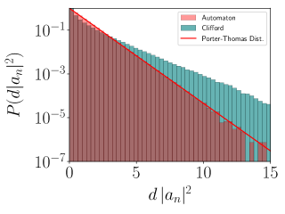
Figure 2: The probability distribution of bit-strings $P(2^{N}|a_{n}|^{2})$ as measured in the $x$-basis, for automaton and Clifford wave functions on $N=16$ sites. The fluctuations of bit-string amplitudes in the automaton wave functions obey the strict bound for unitary $\gamma$ designs given by Eq. (18) up to at least $\gamma\sim N$. The Clifford wave function, on the other hand, only obeys this bound up to $\gamma\sim 3$.

To see this, we simulated the exact quantum circuit dynamics of an initial product state with all spins oriented perpendicular to the computational basis, with gates chosen randomly from our automaton gate set. To compare, we also simulated random Clifford circuits, with gates chosen randomly from $\{CNOT,SWAP,H\}$ and acting on a random initial product state. We should emphasize that since we are interested in the distribution of a many-bit output, we cannot use the polynomial time classical algorithm to simulate either the automaton or Clifford circuits Jozsa and den Nest (2013). Instead, we are forced to track the evolution of the entire wave function for a small system size. We simulated a circuit with $L=16$ sites and circuit depth $D=100$. A histogram of the final projective measurement outcomes for both cases is shown in Fig. 2. For the automaton circuit, the state is initialized with all spins oriented perpendicular to the computational basis, and the final output bit-strings are measured in the x-basis. The results are averaged over 100 different circuit realizations.

We see that the probability of different basis strings decays exponentially, up to the resolution we are able to measure. For the Clifford circuits, the Porter-Thomas bound is satisfied only up to $\gamma=3$, but is violated for $\gamma>3$. The implication is that for automaton circuits, measurements in the orthogonal basis are extremely uniform in the same way as for high complexity Haar random states.

III.3 Entanglement and Complexity

The pattern of entanglement in quantum states is very closely related to the quantum state complexity. We will see that the entanglement in states drawn from a unitary k-design must satisfy certain constraints. As shown by Page, nearly all quantum states chosen from the Haar measure will have a nearly maximal amount of entanglement Page (1993). More precisely, the bipartite von Neumann entanglement entropy of a random quantum state with Hilbert space $\mathcal{H}=\mathcal{H}_{A}\otimes\mathcal{H}_{B}$ can be shown to be

$$S_{vN}\geq\log(d_{A})-\frac{1}{2\ln(2)}\frac{d_{A}}{d_{B}}$$ (19)

where $d_{A}\leq d_{B}$ are the dimensions of $\mathcal{H}_{A}$ and $\mathcal{H}_{B}$ respectively.

Our definition of quantum state complexity implies that high complexity states cannot easily be distinguished from the maximally mixed state. This property necessarily requires the state to be nearly maximally entangled, so that the reduced density matrix $\rho_{A}$ is close to the maximally mixed state for all subregions $|A|<\frac{L}{2}$. Therefore, the process of scrambling requires that initially local information becomes stored in the non-local many body entanglement of the wave function. However, the converse statement is not always true. States of high entanglement are not necessarily always of high complexity. To distinguish between states of different complexity, we need to develop more fine grained measures of entanglement.

a)

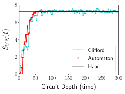
b)

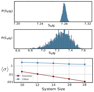
Figure 3: a) The bipartite entanglement entropy $S_{vN}$ as a function of time for both Clifford and automaton circuits. In both cases, the late time entanglement averages to the Haar random ‘Page entropy’, however the temporal fluctuations are significant in the Clifford circuit, while they appear negligibly small in the automaton circuit. b) This uniformity of entanglement can be seen in a single realization of an automaton wave function, if we measure the entanglement in all possible bipartitions of the lattice. We show the probability distribution of the entanglement entropy across the different partitions for the automaton (top) and Clifford (middle) wave functions. The standard deviation of these distributions (bottom), $\langle\sigma\rangle=\sqrt{\langle(S_{vN}-\langle S_{vN}\rangle)^{2}\rangle}$, decays exponentially with system size for automaton circuits and appears to saturate to a constant value for Clifford circuits.

In Fig. 3 a), we show the time evolution of the bipartite von Neumann entanglement entropy $S_{vN}(t)$ for a single circuit realization of both automaton and Clifford circuit types. In both cases, we observe a short regime of linear entanglement growth followed by a late time regime where the entanglement saturates near the volume law Page value $S_{vN}=L/2-1/(2\ln(2))$. The main difference between the two cases is that for the automaton circuit, after reaching saturation, $S_{vN}$ remains very close the exact Page value at all times, while in the Clifford circuit there are relatively large fluctuations in $S_{vN}(t)$. We will argue that these fluctuations in the entanglement entropy are a sign that a state is not drawn from a sufficiently high unitary design.

$S_{vN}$ measures the entropy of the reduced density matrix, $\rho_{A}$, which encodes all information about observables which can be measured locally in region A. Fluctuations in $S_{vN}(t)$ therefore imply there are fluctuations in the value of some measurement in region A. In Brandao et. al. Brandão et al. (2019), it was shown that for a unitary k-design, the higher order moments of a generic expectation value are bounded by

$$\mathbb{E}_{|\psi\rangle}\left[\left(\text{Tr}(M|\psi\rangle\langle\psi|)-\mathbb{E}_{|\psi\rangle}[\text{Tr}(M|\psi\rangle\langle\psi|)]\right)^{k}\right]\leq\left(\frac{k^{2}}{d}\right)^{k/2}.$$

(20)

For a highly complex state, which forms a large k unitary design, the higher order fluctuations on all measurements become very small. If we partition our lattice into regions $A$ and $B$, and let $M$ be any projective measurement implemented on the spins in subsystem $A$, then this should also bound fluctuations of the entanglement entropy. Therefore, the temporal fluctuations in the entanglement entropy are evidence that the Clifford circuit is of lower complexity than the automaton circuit.

Using this intuition, we can develop an entanglement measure which acts on a quantum wave function at a single time and quantifies the degree of the entanglement fluctuations. This measure is simply the full probability distribution of bipartite entanglement entropies measured across all $N\choose N/2$ bipartitions of the lattice. Comparing the entropy across many different lattice partitions effectively measures the multi-partite entanglement of the wave function Amico et al. (2008), similar to the entanglement measure developed by Meyer and Wallach Meyer and Wallach (2002).

We show the histogram of these entropies in Fig. 3b) for both automaton and Clifford circuits. We see that indeed, for automaton circuits, almost all bipartitions of the state have the same entanglement entropy, which is very close to the Page entropy. However, for Clifford circuits, while the average entanglement entropy is equal to the Page entropy, there are significant, $O(1)$, variations in this measurement depending on which bipartition is selected. This implies that the Clifford states are much less uniform than the automaton wave functions. Therefore, the variance in measurements in automaton states should satisfy Eq. 20 for a much higher value of $k$ compared to Clifford states.

Perhaps the most direct connection between entanglement and unitary design can be made by studying the generalized Renyi entanglement entropies. In Liu et al. (2018a), it was shown that the higher order $\alpha$-th Renyi entropies can be used as a direct probe of the design order. The $\alpha$-Renyi entropy is defined as

$$S^{\alpha}(\rho_{A})=\frac{1}{1-\alpha}\log(\text{Tr}[\rho_{A}^{\alpha}])=\frac{1}{1-\alpha}\log\left[\sum_{i}\lambda_{i}^{\alpha}\right],$$ (21)

where $\lambda_{i}$ are the eigenvalues of the reduced density matrix $\rho_{A}$. As $\alpha\rightarrow\infty$, $S^{\alpha}(\rho_{A})=S_{\min}(\rho_{A})=-\log(\lambda_{\max})$, approaches the min entropy. $S_{\min}(\rho_{A})$ simply probes the largest eigenvalue of $\rho_{A}$, and bounds all other Renyi entropies $S^{\alpha}(\rho_{A})\leq S_{\min}(\rho_{A}),\forall\alpha$. In Liu et al. (2018a), it was shown that the $\alpha$-Renyi entropy averaged over a unitary $\alpha$-design is nearly maximal. Therefore, the higher-order Renyi entropies can be seen as a probe of higher order complexity in the wave function. It was shown that

$$\mathbb{E}_{\nu_{k}}\left[S^{k}(\rho_{A})\right]\geq d_{A}+\mathcal{O}(1).$$ (22)

where $\mathbb{E}_{\nu_{k}}$ is the average over the k-design distribution of unitary matrices. Furthermore, they showed that

$$\mathbb{E}_{\nu_{k}}\left[\text{Tr}\{\rho_{A}^{k}\}\right]=\mathbb{E}_{\text{Haar}}\left[\text{Tr}\{\rho_{A}^{k}\}\right].$$ (23)

In other words, the $k-th$ Renyi entropies are all nearly maximal up to an $\mathcal{O}(1)$ constant for a unitary k-design, and the trace of $\rho_{A}^{k}$ exactly equals the Haar random value. This exact equality does not hold in general for the Renyi entropies since the log of an average does not in general equal the average of a log.

We measure the different Renyi entropies for Haar random local circuits, automaton circuits and Clifford circuits. In all cases, we again perform the measurements on small circuits where we can track the evolution exactly. In principle, we could measure these Renyi entropies for larger automaton circuits using our classical algorithm. However, this involves measuring higher order ‘Swap’ operators, which have a value which is exponentially small in the amount of entanglement. Since the amount of entanglement of a bipartition grows like a volume law, this measurement becomes exponentially hard in these systems.

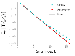
Figure 4: The average trace of $\rho_{A}^{k}$ for different values of the Renyi index k. We find that the expectation over circuits of $\text{Tr}(\rho_{A}^{k})$, is equal to the Haar random value for automaton circuits for all $k$ that we tested. For Clifford circuits, which form a unitary 3-design, $\mathbb{E}[\text{Tr}(\rho_{A}^{k})]$ are only constrained to match the Haar random value up to $k=3$, and show significant deviation above $k\approx 5$.

In Fig. 4, we show the expectation value for the k${}^{\text{th}}$ Renyi entropy, as measured in both automaton and Clifford circuits. Amazingly, the expectation value for the automaton wave functions is exactly equal to the Haar random value for all values of $k$ which we measured. For Clifford circuits, on the other hand, the expectation value matches the Haar value for low Renyi index, but deviates significantly at higher value of $k$. $\mathbb{E}_{\nu}[\rho_{A}^{k}]$ is the expectation value of the k${}^{\text{th}}$ Renyi entropy measured over the ensemble of circuits $\nu$. At high Renyi index, $k$, small fluctuations away from this mean will be amplified. Therefore, these results are again consistent with the hypothesis that fluctuations of random measurements are highly suppressed in automaton wave functions, to the extent that such measurements mimic that of a fully Haar random wave function. Interestingly, in Liu et al. (2018b), it was found that the infinite order Renyi entropy $S_{\infty}\sim-\log(|\lambda_{max}|)$, saturates near its maximal value after only an $O(N)$ time. Such a state is known as ‘max scrambled’. Although the complexity of the quantum state continues to grow past the max scrambling time, all max scrambled states will appear maximally complex according to the Renyi entanglement measures. Our results strongly imply that automaton wave functions will become max scrambled for polynomial depth circuits.

III.4 Entanglement Spectrum

Entanglement spectrum is the name given to the statistical distribution of the eigenvalues of a reduced density matrix Li and Haldane (2008); Geraedts et al. (2016). The spacing between these eigenvalues form a distribution which is known for different ensembles of random matrices Mehta (2004) and generically follows a Wigner-Dyson distribution. For a random $U(N)$ unitary matrix, the spacing between eigenvalues follows the Gaussian unitary ensemble (GUE). These Wigner-Dyson distributions have the special property that there is repulsion between neighboring eigenvalues. On the other hand, the reduced density matrix of wave functions that result from integrable dynamics do not, in general, form a random matrix. In such a case, the eigenvalues of $\rho_{A}$ do not show the same degree of level repulsion and may follow a simple Poisson distribution.

To measure the entanglement spectrum, we first rewrite the wave function $|\psi\rangle$ using the Schmidt decomposition.

$$|\psi\rangle=\sum_{i}\lambda_{i}|\alpha_{i}\rangle|\beta_{i}\rangle$$ (24)

where $\lambda_{i}$ are real positive numbers.

We can then define the entanglement spacing, $s_{i}=\lambda_{i+1}^{2}-\lambda_{i}^{2}$, where we order the Schmidt coefficients such that $\lambda_{0}\leq\lambda_{1}\leq\cdots\leq\lambda_{M}$. For convenience Atas et al. (2013); Oganesyan and Huse (2007), we define the level spacing ratio

$$r_{i}=\min\left[\frac{s_{i}}{s_{i+1}},\frac{s_{i+1}}{s_{i}}\right].$$ (25)

The entanglement spectrum is then the probability distribution of the $r_{i}$ random variables.

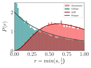
Figure 5: The level spacing distribution of the entanglement spectrum for automaton wave functions show Wigner-Dyson GUE statistics, while the Clifford states show Poisson like statistics. Wigner-Dyson statistics are expected for the eigenvalue distribution of random matrices and are a signature of quantum chaos.

In Fig. 5, we show the entanglement spectrum statistics for wave functions that result from both the automaton circuit and Clifford circuits. We see that the spectrum in the automaton case follows very closely the universal form of the Gaussian unitary ensemble Atas et al. (2013); Buijsman et al. (2019), while the Clifford states do not show the same level repulsion and appear to follow a Poisson distribution.

The relationship between chaotic dynamics and entanglement spectrum has been studied in Shaffer et al. (2014); Chamon et al. (2014); Yang et al. (2017). However, a complete theoretical understanding of the connection between quantum state complexity and the entanglement spectrum is still lacking. In Shaffer et al. (2014), it was noted that dynamics under a universal set of quantum gates is sufficient to generate $GUE$ statistics of the entanglement spectrum, while evolution under Clifford gates results in Poisson statistics. Here, we have shown that this condition of a universal set of quantum gates is not necessary to generate GUE statistics. Indeed, we have created a state with such statistics using only the automaton gate set, which can be simulated classically in the way outlined in section II. It is interesting that such signatures of quantum chaos also appear in wave functions which can be simulated classically.

It remains an open question whether there is a concrete relationship between entanglement statistics and unitary k-designs.

IV Measuring Complexity in Automaton Circuits

IV.1 Generalized Out-Of-Time-Ordered Correlators

Out-of-time-ordered correlators (OTOCs) have recently been found to be an important tool for characterizing operator spreading in quantum circuits. The 4-point OTOC

$$\langle OTOC^{(4)}\rangle=\langle A(t)B(0)A(t)B(0)\rangle$$ (26)

measures the average degree of non-locality of an operator $A(t)=U^{\dagger}AU$, and has been extensively studied in the context of thermalization and quantum chaos Hosur et al. (2016); Nahum et al. (2018); Maldacena et al. (2016). This quantity will only be small if $A(t)$ evolves into a highly non-local operator. In Hosur et al. (2016), it was shown that the information-theoretic definition of scrambling is implied by the generic decay of this four point function. Furthermore, any initial product state which is evolved by such a unitary can be shown to be nearly maximally entangled.

Following the work of Roberts and Yoshida Roberts and Yoshida (2017), we can generalize this operator and define the 2k-point out-of-time ordered correlators:

$$\langle OTOC^{(2k)}\rangle=\langle A_{1}(t)B_{1}(0)\dots A_{k}(t)B_{k}(0)\rangle.$$ (27)

Deep connections have been found between the generic smallness of the 2k point functions, unitary k-designs and quantum circuit complexity. A generic 2k-point function contains k copies of $U$ and k copies of $U^{\dagger}$. Therefore, if $U$ is sampled from a unitary k-design then the average of the 2k-point function over the ensemble $\{U\}$ must equal the Haar random value, and therefore will be exponentially small. Since the four-point OTOC expectation value is quadratic in the $U$ and $U^{\dagger}$ operators, we see that only a unitary 2-design is necessary for scrambling. We know, however, that the complexity of the wave function will continue to grow well past this scrambling time.

These higher order correlators are therefore an important tool for understanding complexity beyond scrambling in quantum dynamics. Crucially, the generalized OTOC functions give us a probe which is insensitive to the onset of lower-order forms of complexity. For example, the 4-point function in local circuits takes on an $O(1)$ value throughout the ‘thermalization’ regime, before decaying to an exponentially small value after a time $t^{*}\sim O(L)$ for local circuits. This is in contrast to the entanglement entropies, which can also be used to diagnose scrambling and complexity, but which always require an exponentially hard measurement to implement. This feature of the OTOCs is both useful experimentally, and critically, allows us to use automaton circuits to numerically probe the onset of complexity efficiently in large systems.

We can therefore use these higher order correlation functions to probe the structure of the wave functions output from quantum circuits. If we can find a 2k-point OTOC which is nonzero, this implies that the unitary ensemble is not a k-design and the wave function is likely of lower complexity.

In Roberts and Yoshida (2017), it was shown that the average value of the 2k-point correlation function can directly give a lower bound for the quantum circuit complexity of a unitary ensemble $\{U\}=\varepsilon$,

$$C(\varepsilon) \geq (2k-1)2N$$ (28)

$$-\log\left[\sum_{A_{1}\dots B_{1}\dots}\langle A_{1}(t)B_{1}\dots A_{k}(t)B_{k}\rangle\right].$$

This expression is useful for showing that there is a direct connection between the generic decay of the higher-order OTOCs and circuit complexity. Unfortunately, it is not very useful for numerically calculating a bound on circuit complexity since the main contribution comes from calculating a sum over an exponentially large number of operators each of which is in general exponentially small. As we will explain below, in this work, we take an alternative route by identifying special structured OTO correlators which have an $O(1)$ value for low complexity dynamics.

We will proceed as follows. We first identify a class of k-order OTOCs which have a special recursive structure which can be physically motivated and can be easily generalized. We then also perform a brute force search over all 2k-point OTOCs for a fixed value of k. These correlators are not as easily generalizable, but give a more complete picture of complexity growth in local random circuits. In both cases, we are able to efficiently measure the correlation function in high depth automaton circuits with a large number sites. We find that in both cases the correlators eventually decay to an exponentially small value in automaton circuits, providing strong evidence in very large systems that automaton circuits produce high complexity wave functions. Further, our brute force search is able to identify a large, linear in $k$, regime where the quantum wave function appears scrambled but the higher order OTOCs have not yet decayed. This gives us an unprecedented ability to numerically study complexity growth in local quantum circuits.

IV.2 Recursive K-point Functions

We begin by studying a special instructive class of k-point OTOC functions which often retain an $O(1)$ expectation value beyond the scrambling time $t_{sc}$. In these correlators, the time evolved Heisenberg operators $\tilde{\mathcal{O}}=\mathrm{U}^{\dagger}\mathcal{O}\mathrm{U}$ can be treated as a generalized unitary operator $\mathrm{U}^{(n)}$:

$$\mathrm{U}^{(0)} = \mathrm{U}$$ (29)

$$\mathrm{U}_{\mathcal{O}}^{(1)} = \mathrm{U}^{\dagger}\mathcal{O}\mathrm{U}$$ (30)

$$\mathrm{U}_{\mathcal{O},\mathcal{O}^{\prime}}^{(2)} = \mathrm{U}^{(1)^{\dagger}}_{\mathcal{O}}\mathcal{O}^{\prime}\mathrm{U}_{\mathcal{O}}^{(1)}$$

$$\dots$$

The higher order OTOCs can be interpreted as assessing the scrambling properties of $\mathrm{U}^{(n)}$. For example, for we can write

$$\left\langle\,\tilde{A}B\tilde{A}C\tilde{A}B\tilde{A}C^{\phantom{\dagger}}\right\rangle = \left\langle\mathrm{U}^{(1)\dagger}_{A}B\mathrm{U}^{(1)}_{A}\,C\,\mathrm{U}^{(1)\dagger}_{A}B\mathrm{U}^{(1)}_{A}\,C\right\rangle$$ (32)

$$= \left\langle\,B(t)CB(t)C^{\phantom{\dagger}}\right\rangle.$$

where, following the notation of Roberts and Yoshida (2017), we let $\tilde{A}=\mathrm{U}^{\dagger}A\mathrm{U}$. Therefore, this 8-point function under $\mathrm{U}$ can be thought of as a 4-point function under $\mathrm{U}^{(1)}$. These recursive OTOCs can always be interpreted as 4-point OTOCs with additional local operators hiding in the generalized unitaries.

Under a fully Haar random $U(2^{N})$ dynamics, all k-point correlation functions will decay to an exponentially small value. Therefore, not only does $\mathrm{U}$ have high quantum complexity, but so do the operators, $\mathrm{U}^{(1)}=\mathrm{U}^{\dagger}A\mathrm{U}$, $\mathrm{U}^{(2)}=\mathrm{U}^{(1)\dagger}B\mathrm{U}^{(1)}$, etc.

Conversely, for the known examples of exact unitary designs, such as the ensemble of Pauli strings and Clifford circuits, the higher order generalized unitaries are of lower complexity than the original operator.

Consider the case where $\{\mathrm{U}\}$ is an ensemble of Clifford circuits. These are known to form a unitary 2-design in general, and a 3-design when the local Hilbert space is qubits, but never form a 4-design Zhu et al. (2016). Therefore, when averaged over the ensemble of all Clifford circuits, all 4-point functions are found to be exponentially small, $\langle\tilde{A}B\tilde{A}B\rangle=4^{-N}$. However, the defining feature of Clifford circuits is that they evolve Pauli strings to other Pauli strings. Therefore, the generalized unitary operator $\mathrm{U}^{(1)}$ is simply a Pauli string, $\mathrm{U}^{(1)}=\mathrm{S}=\otimes_{i}\sigma_{i}^{\alpha_{i}}$. The ensemble of Pauli strings $\{\mathrm{S}\}$ are known to merely form a 1-design, and so the 4-point functions under $\{\mathrm{U}^{(1)}\}$ do not decay to zero. The 4-point function under $\mathrm{U}^{(1)}$ is an 8-point function under $\mathrm{U}$. Therefore, there always exist 8-point functions for Clifford circuits which do not decay to the Haar random value. Therefore, the fact that Clifford circuits merely scramble is demonstrated by the fact that that while $\{\mathrm{U}\}$ scrambles, the ensemble of unitary operators $\{A(t)=\mathrm{U}^{\dagger}A\mathrm{U}\}$ do not. In this way, the higher order OTOCs expose a hierarchical structure of unitary designs.

With this understanding, we use the higher order OTOC to probe the dynamics of automaton circuits in the ‘beyond scrambling’ regime. Since automaton circuits apply nontrivial dynamics in the direction perpendicular to the computational basis, we further define a set of recursive unitaries which are composed only of single site $X$ Pauli operators:

$$\mathrm{U}^{(0)} = \mathrm{U}$$

$$\mathrm{U}_{i_{1}}^{(1)} = \mathrm{U}^{\dagger}X_{i_{1}}\mathrm{U}$$

$$\mathrm{U}_{i_{1}i_{2}}^{(2)} = \mathrm{U}^{(1)\dagger}_{i_{1}}X_{i_{2}}\mathrm{U}^{(1)}_{i_{1}}$$

$$\mathrm{U}_{i_{1}i_{2}\dots i_{m}}^{(m)} = \mathrm{U}^{(m-1)\dagger}_{i_{1}i_{2}\dots i_{m-1}}X_{m}\mathrm{U}^{(m-1)}_{i_{1}i_{2}\dots i_{m-1}}.$$

We then write down the special class of generalized OTOCS

$$F^{(2^{k})}_{i_{1},\dots,i_{k-1},0} = \langle\mathrm{U}^{(k-1)\dagger}_{i_{1}\dots i_{k-1}}X_{0}\mathrm{U}^{(k-1)}_{i_{1}\dots i_{k-1}}X_{0}\rangle.$$ (33)

Then, for example:

$$F^{(4)}_{L,0} = \langle\tilde{X}_{L}X_{0}\tilde{X}_{L}X_{0}\rangle,$$

$$F^{(8)}_{L,1,0} = \langle\tilde{X}_{L}X_{1}\tilde{X}_{L}X_{0}\tilde{X}_{L}X_{1}\tilde{X}_{L}X_{0}\rangle.$$ (34)

$F^{(4)}_{L,0}$ is simply the usual 4-point OTOC which measures operator scrambling, so that $F^{(4)}_{L,0}=1$ if and only if $[\tilde{X}_{L},X_{0}]=0$. On the other hand, $F^{(8)}_{L,1,0}$ measures the scrambling of $X_{1}$ under a time evolution by $\tilde{X}_{L}=\mathrm{U}^{\dagger}X_{L}\mathrm{U}$. In this case, we have that $F^{(8)}_{L,1,0}=1$ if either $[\tilde{X}_{L},X_{0}]=0$ or $[\tilde{X}_{L},X_{1}]=0$, and therefore we have that

$$\mathbb{E}[F^{(8)}_{L,1,0}]\geq\mathbb{E}[F^{(4)}_{L,0}].$$ (35)

These higher order OTOCs are a more strict measure of complexity, can easily be generalized, and retain a simple interpretation as measuring the scrambling properties of the generalized unitary operators.

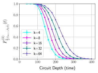
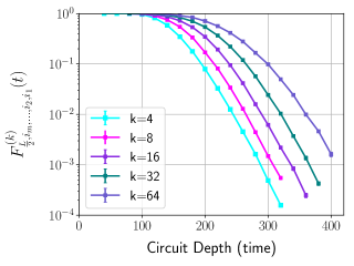
Figure 6: The recursive k${}^{\text{th}}$ order OTO correlators, $\langle\text{F}_{\frac{L}{2},i_{m},\dots,i_{2},i_{1}}^{(k)}\rangle$, defined in Eq. (33), for a system with $L=100$ sites with periodic boundary conditions. These OTOCs are composed of single site Pauli $X$ operators acting on sites $\{\frac{L}{2},i_{m},\dots,i_{3},i_{2},i_{1}\}=\{\frac{L}{2},\log_{2}(k/2),\dots,2,1,0\}$. See Eq. (34), for the form of the $k=4$ and $k=8$ operators. We can measure these correlators for very high values of k. (Top) The higher order OTOCs decay at progressively later times. The highest order OTOCs, remain nonzero well past the scrambling time. (Bottom) At late times, all correlators eventually decay at an exponential rate.

We measure these recursively defined operators and show the results in Fig. 6, for an automaton circuit with $L=100$ sites. The results are again averaged over different random circuit realizations. We point out several important features of this data.

First, we see that for automaton circuits, all generalized OTOC functions do eventually decay to an exponentially small value. We take this as important further evidence that automaton circuits have high quantum circuit complexity and the resulting wave functions have a high quantum state complexity. Again, this should be seen as a stark contrast to other examples of numerically tractable quantum circuits such as Clifford circuits, for which we can always find higher order OTOCs which do not decay at all.

Second, we see that in these circuits, the higher order OTOCs are nonzero at later times than the usual 4-point function $F^{(4)}_{L,0}=\langle\tilde{X}_{L}X_{0}\tilde{X}_{L}X_{0}\rangle.$ This concretely demonstrates that in such local random circuits there exists a well defined regime beyond the scrambling time where information about the original state $|\psi_{0}\rangle$ is not completely lost. In these ‘intermediate complexity states’, local information from $|\psi_{0}\rangle$ can still be probed using these special measurements. Further, note that the expectation value of the higher order OTOCs at late times is generally much greater than twice the previous order, yet only requires twice the computational effort to measure.

Finally, we see that the ‘scrambling time’, $t^{*}$ for this class of higher order OTOCs appears to only increase logarithmically with order $k$. In particular, we find that

$$t^{*}=v_{B}L+v_{k}\log_{2}(k)$$ (36)

In the next subsection, we will see that this is not a generic feature of the higher order OTOCs.

IV.3 Higher Order OTOCs and Complexity

A more complete picture of complexity growth in our local random automaton circuits can be found by studying more general classes of k-point OTOCs.

For local random circuits, it was shown in Brandão et al. (2016), that the unitary design order will continue to grow far beyond the scrambling time. It is expected that the complexity in these local circuits grows linearly with circuit depth, $D$, for an exponentially long time Brown and Susskind (2018). This linear complexity growth is of great interest in the high-energy literature. In the context of the AdS/CFT correspondence, the linearly growing complexity of the dual CFT is related to the growth of an AdS wormhole Susskind (2016); Stanford and Susskind (2014). In Brandão et al. (2016), a weaker result, that design order, (and therefore the complexity), in these circuits grows at least like the polynomial $D^{\frac{1}{11}}$, was proven rigorously. Linear complexity growth can also be rigorously shown in the limit of a large local Hilbert space dimension Brandão et al. (2019). However, there is no known proof of linear complexity growth for the more difficult case of a local random circuit composed of qubits.

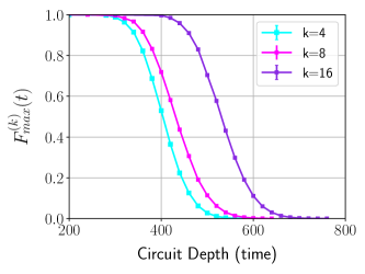
Figure 7: A brute force search over a wide class of k${}^{\text{th}}$ order OTOCs gives the max OTOC $F_{max}^{(k)}$ (see text for a precise definition). We see that the $k=16$ point function decays at a much later time in this case compared to the recursive OTOCs of the previous section. In the bottom plot, we show the same data on a logarithmic scale and define the scrambling time $t^{*}_{k}(\epsilon)$ as the time beyond which $F_{max}^{(k)}<\epsilon$. In the inset we see that the ratio between scrambling times $\Delta=(t^{*}_{16}-t^{*}_{8})/(t^{*}_{8}-t^{*}_{4})$ approaches $\Delta=2$ as $\epsilon\rightarrow 0$.

Quantum automaton circuits allow us to test this conjecture numerically in large systems by using the generalized OTOC operators as a measure of complexity. To do this, we should search over the full set of out-of-time-ordered operators

$$OTOC_{max}^{(k)}=\max_{A_{1},B_{1},\dots,A_{k},B_{k}}\mathbb{E}_{\nu}\left[\langle\tilde{A}_{1}B_{1}\dots\tilde{A}_{k}B_{k}\rangle\right]$$ (37)

where $A_{i}$, $B_{i}$ are any Pauli string operators. However, this would require computing $4^{Nk}$ different expectation values, which is clearly intractable even for small values of $N$ and $k$.

Instead, we again restrict the operators $A_{i}$, $B_{i}$, to be only single site Pauli $X$ operators and define

$$F_{max}^{(k)}=\max_{i_{1},\dots,i_{k}}\mathbb{E}_{\nu}\left[\langle\tilde{X}_{i_{1}}X_{i_{2}}\dots\tilde{X}_{i_{2k-1}}X_{i_{2k}}\rangle\right].$$ (38)

In practice, we find a lower bound for this operator by searching only over operators with support on a small fixed number of sites. Even with these practical restrictions, $F_{max}^{(k)}(t)$ gives an upper bound on the design order of the circuit at time $t$.

For $k$ up to $k=16$, we search over all possible correlators with $A_{i},B_{i}\in\{X_{0},X_{1},X_{L/2-1},X_{L/2}\}$. For $k=4$, the maximum OTOC is the usual 4-point function $F_{max}^{(4)}=\langle\tilde{X}_{L/2}X_{0}\tilde{X}_{L/2}X_{0}\rangle$. At $k=8$, we find the maximum expectation value occurs when the OTOC takes the form

$$F_{max}^{(8)} = \langle\tilde{\mathcal{O}}\tilde{\mathcal{O}}\rangle$$ (39)

$$\tilde{\mathcal{O}} = \tilde{X}_{0}X_{\frac{L}{2}}\tilde{X}_{0}X_{0}$$ (40)

To calculate $F_{max}^{(16)}$, we must measure $\sim 32000$ different correlation functions. In this case, we find that the maximum expectation value occurs for

$$F_{max}^{(16)} = \langle\tilde{\mathcal{O}}\tilde{\mathcal{O}}\rangle$$ (41)

$$\tilde{\mathcal{O}} = \tilde{X}_{0}X_{\frac{L}{2}}\tilde{X}_{0}X_{0}\tilde{X}_{0}X_{\frac{L}{2}}\tilde{X}_{\frac{L}{2}}X_{0},$$ (42)

plus special equivalent permutations of these operators which are related by symmetry.

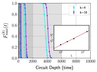
Figure 8: $F_{max}^{(k)}(t)$ for $k=4$ and $k=16$ for different system sizes $L=100,400,1600$ (Shown left to right in separate shaded regions). The gap between the $k=4$ and $k=16$ wave fronts grows with system size. This gap size vs $L$ is shown in the inset to grow like $\Delta\sim L^{\alpha}$ with $\alpha=0.48(1)$.

Note that we find this correlation function appears to ‘peak’ only at special values of $k$. That is, we find that at late times, $F_{max}^{(16)}(t)\gg F_{max}^{(8)}(t)\gg F_{max}^{(4)}(t)$, but that this is not true for other values of $k$ which we tested (up to at least k=24).

The results for the 4, 8 and 16 point functions are shown in Fig. 7. Again, we see that all correlation functions we measured decay to an exponentially small value at late times. The dramatic difference is that the $k=16$ point function remains nonzero for a significantly longer period of time.

We see that the complexity growth in local random circuits is subject to the so called switchback effect Stanford and Susskind (2014), whereby there is a delay in the onset of linear complexity growth for initially local operators. This occurs due to the exact cancellation of unitary gates outside the lightcone in the operator evolution $\tilde{\mathcal{O}}=\mathrm{U}^{\dagger}\mathcal{O}\mathrm{U}$.

We define the time $t^{*}_{k}(\epsilon)$ as the circuit depth beyond which $F^{(k)}_{max}<\epsilon$. Due to the switchback effect, we expect that the linear complexity growth begins only after we reach the scrambling time $t_{sc}=t^{*}_{4}$, when the wave function forms an approximate 2-design. At some later time $t^{*}_{8}$, we will have $F_{max}^{(8)}<\epsilon$, and the wave function will form an approximate 4-design. This difference $\Delta=t^{*}_{8}-t^{*}_{4}$ defines the rate of complexity growth. The inset in Fig. 7 b) shows that $t^{*}_{16}-t^{*}_{8}\approx 2\Delta$ for sufficiently small $\epsilon$. In Fig. 8, we find that as the system size in increased, the size of the ‘complexity gap’ $\Delta$ grows like $\sqrt{(}L)$.

Therefore, at least for these 3 values of $k$, the generalized scrambling time appears to follow the form

$$t^{*}=v_{B}L+\Delta\sqrt{L}\,k.$$ (43)

The linear growth with $k$ is consistent with a linear growth of design order (and therefore complexity) with circuit depth. That is, we show that for the values of $k$ studied here, there exists a regime beyond scrambling in local random circuits where the wave function is definitively not a (k/2)-design, and the size of this regime appears to grow linearly with k.

V Discussion

In this paper, we have studied in detail the quantum state complexity of wave functions which are the output of local automaton circuits. These gates act very simply on computational basis states, which allows us to simulate these circuit efficiently using a classical computer. Despite this, when acting on an initial product state with spins oriented perpendicular to the computational basis, local random automaton circuits generate very complex highly entangled quantum wave functions.

We can quantify the complexity of the wave functions using tools from quantum information theory. We specifically relate the quantum state complexity to the difficulty of distinguishing the wave function from the maximally mixed state. We considered several different measurements in order to argue that the ensemble of automaton wave functions form an approximate projective unitary design of high order. Based on known connections between unitary designs and quantum complexity, these results imply that automaton wave functions have a high quantum state complexity.

In the first section, we considered four basic measures of complexity. First, we saw that in quantum automaton circuits, the distribution of bit-strings (which result from many-qubit projective measurements in a basis orthogonal to the computational basis) follows the well known ‘Porter-Thomas’ distribution up to the resolution of our numerics. Second, we characterized von Neumann entanglement entropy across all possible bipartitions of the lattice and found that it is always nearly exactly equal to the Page entropy. This is in contrast to Clifford circuits, which show significant fluctuations between different partitions. We also studied the level spacing distribution in the entanglement spectrum and saw a convergence to the Gaussian unitary ensemble (GUE) Wigner-Dyson distribution, a result that implies the reduced density matrix of automaton wave functions behave like random matrices. Finally, we studied the generalized k-th Renyi entropies, which were shown in Liu et al. (2018a) to be a direct probe of unitary design complexity. We found that for automaton wave functions, the k-th Renyi entropy was exactly equal to the Haar random value for all values of $k$ we measured. This suggests that design complexity in automaton wave functions will grow until the infinite order limit of the Renyi entropy is saturated, a condition known as ‘max scrambling’.

By every metric, the automaton circuits exhibit the same properties as a wave function from high depth local random circuit composed of universal basic gates. Such circuits are known to form an approximate polynomial unitary design and therefore at sufficient depth approximate the fully Haar random wave functions to arbitrary accuracy. All the above results suggest that fluctuations in automaton wave functions are highly suppressed in the same way as in universal random circuits. In fact, the bit-string distribution and generalized Renyi entropies follow the constraints imposed for large k projective k-designs, implying that automaton wave functions approximate at least the first $k$ moments of the fully random Haar measure. Further, convergence of the bit-string distribution to the Porter-Thomas form and the entanglement level spacing to the Wigner-Dyson distribution are often cited as key signatures of quantum chaos. Throughout, we compared the results for automaton circuits to those of Clifford circuits which are known to form only a finite low order unitary design, even for high depth circuits. This comparison serves to highlight the difference between high and low complexity states.

In the second section, we studied the $2k$-point out-of-time-ordered correlation (OTOC) functions. These are a generalization of the popular 4-point OTOC, which is known to characterize the onset of scrambling in quantum systems. Unlike the previous set of measurements which require an exponential effort to compute using our quantum Monte Carlo algorithm, the generalized OTOC functions are capable of probing complexity beyond the scrambling regime using computational resources which scale linearly with system size. Therefore, we can use these as a tool to efficiently study complexity growth in very large circuits.

We first identified a set of recursively defined 2k-point OTOCs whose precise form is physically motivated and which can be easily generalized to very high values of $k$. We argue that in low complexity unitary circuits, such as Clifford circuits, these higher order recursive OTOCs do not generically decay. In automaton circuits, however, we find that at some time $t^{*}$ beyond the scrambling time these correlation functions always decay to an exponentially small value. This is both further evidence that automaton wave functions form projective unitary designs and proof that generalized OTOCs can be practically used to probe complexity beyond scrambling in large systems.

Importantly, using automaton circuits, we were also able to study more generic forms of out-of-time ordered correlation functions. By searching over thousands of possible k-point OTOCs up to $k=16$, we were able to identify special orderings of operators for which the average correlators remain nonzero for a far longer time even than the recursive OTOCs discussed above. Measuring these special OTOCs gives us an unprecedented ability to numerically characterize the rate of complexity growth in large local random circuits. In particular, we found that the scrambling time for the k-th order OTOC appears to increase linearly with $k$. Notably, this result is consistent with the linear growth of complexity which is conjectured in the literature.

Taken together, all of the above results are very strong evidence that the automaton circuits are capable of producing wave functions with high quantum state complexity. Our results therefore imply that automaton circuits are a rare example of a numerically tractable system which can generically simulate quantum chaotic dynamics on a classical computer. We expect there to be a wide variety of applications across a wide range of fields. Already, this technique has been applied to a range of quantum circuit models in the context of understanding quantum dynamics in systems with different symmetries Iadecola and Vijay (2020); Feldmeier et al. (2020); Iaconis et al. (2019); Chen et al. (2020). We predict that it will become a prominent technique for studying generic chaotic circuit dynamics and may be an important tool for understanding how the growth of complexity beyond scrambling plays a role in thermalizing condensed matter systems. There also exist obvious applications to quantum information theory, where characterizing the complexity of local circuits is a key problem. Beyond this, our work may be useful for practical quantum information processing tasks such as randomized benchmarking Magesan et al. (2011); Wallman and Flammia (2014) and decoupling Szehr et al. (2013), where unitary designs play a key role. The ability of OTOCs to identify unique observables in high depth random circuits which are fully scrambled may be useful experimentally for characterizing the fidelity of non-Clifford quantum circuits. In high energy physics, characterizing the rate of complexity growth in quantum systems is conjectured to be related, through the holographic principle, to the growth of the volume in the bulk geometry beyond the event horizon in black holes. Future work in identifying the specific form of higher order OTOCs which best characterize the complexity growth may therefore shed important insight into these problems.