When Probabilistic Shaping Realizes Improper Signaling for Hardware Distortion Mitigation

Abstract

Hardware distortions render drastic effects on the performance of communication systems. They are recently proven to bear asymmetric signatures; and hence can be efficiently mitigated using IGS, thanks to its additional design degrees of freedom. Discrete AS can practically realize the IGS by shaping the signals’ geometry or probability. In this paper, we adopt the PS instead of uniform symbols to mitigate the impact of HWDs and derive the optimal maximum a posterior detector. Then, we design the symbols’ probabilities to minimize the error rate performance while accommodating the improper nature of HWD. Although the design problem is a non-convex optimization problem, we simplified it using successive convex programming and propose an iterative algorithm. We further present a HS design to gain the combined benefits of both PS and GS. Finally, extensive numerical results and Monte-Carlo simulations highlight the superiority of the proposed PS over conventional uniform constellation and GS. Both PS and HS achieve substantial improvements over the traditional uniform constellation and GS with up to one order magnitude in error probability and throughput.

I Introduction

Exponentially rising demands of high data rates and reliable communications given the limited power and bandwidth resources impose enormous challenges on the next generation of wireless communication systems [1, 2]. Various research contributions propose new configurations and novel techniques to address these challenges [3, 4]. Nonetheless, the performance of such systems can be highly degraded by the hardware imperfections in radio frequency (RF) transceivers [5, 6, 7]. Such imperfections give rise to additive signal distortions emerging from the phase noise, mismatched local oscillator, imperfect high power amplifier/low noise amplifier, non-linear amplitude-to-amplitude and amplitude-to-phase transfer [8, 9, 10, 11, 12, 13, 14]. Various contributions emphasized the distinct improper behavior of these hardware distortions [15, 16, 17, 18], which requires effective compensation techniques to meet the performance demands.

I-A Motivation

The improper Gaussian signaling (IGS) is proven as an effective scheme to mitigate the deteriorating effects due to the existence of improper noise or interference in wireless communication systems. More precisely, IGS is a generalized complex signaling that allows the signal components to be correlated and/or to have unequal power, as opposed to proper Gaussian signaling[19]. IGS offers an additional degrees of freedom (DoF) in signaling design characterized by the circularity coefficient [20]. Several studies highlight the significance of IGS to improve the system performance under improper interference [21, 22, 23, 24, 25, 26, 27, 28]. Recent studies quantified the impact of IGS in dampening improper noise effects in multi-antenna or multi-nodal system settings [29, 30, 31, 32, 17, 33], IGS has emerged as promising candidate to improve the average achievable rate performance in multi-antenna systems suffering from HWD [30, 31]. Moreover, IGS benefits can also be reaped in various full-duplex/half-duplex relay settings by effectively compensating the residual self-interference, inter-relay interference and/or HWD [32, 17, 33]. Additionally, the ergodic rate maximization and outage probability minimization based on a generalized error model for hardware impairments in single-input multiple-output (SIMO) and multiple-input multiple-output (MIMO) systems is studied in [31, 30].

I-B Background

Despite the overwhelming benefits of IGS, it is practically infeasible owing to the high detection complexity and unbounded peak-to-average power ratio [34, 2]. This motivated the researchers to design some equivalent finite and discrete asymmetric signaling (AS) schemes for practical implementation. Improper discrete constellation, or AS, entails redesigning the symmetric discrete signal constellation to convert it into an asymmetric signal [2]. Several studies focused on geometric shaping (GS) as a possible designing scheme to improve system performance. GS transforms equally spaced symbols to unequally spaced symbols (due to correlated and/or unequal power distribution between quadrature components of the symbols) in a distinct geometric envelop such as ellipse [35], parallelogram [36, 34] or some irregular envelop [37]. A family of improper discrete constellations generated by widely linear processing of a square $M$-ary quadrature amplitude modulation (QAM) depict parallelogram envelop [34]. Similarly, GS based on optimal translation and rotation also yields parallelogram envelop [36]. However, conditioned on high signal-to-noise ratio (SNR) and higher order QAM, the optimal constellation is the intersection of the hexagonal lattice/packing with an ellipse where the eccentricity determines the circularity coefficient [35]. GS has emerged as a competent player to reduce shaping loss and improve reception at lower signal-to-noise ratios in terrestrial broadcast systems [38, 39]. GS parameters can be designed for diverse objectives such as capacity maximization [34], bit error rate (BER) reduction [36], and symbol error probability minimization [35]. Although the asymmetric discrete family of constellations is practical, they exhibit two types of loss, i.e., shaping loss and packing loss in approaching IGS theoretical limits [34].

I-C Related Work

Most of the efforts to close the gap between AS and ideal IGS are concentrated around GS with a limited focus on probabilistic shaping (PS) as another way to implement AS for HWD. Given a fixed number of symbols and the symbol locations, an asymmetric constellation can be obtained by adjusting the symbol probabilities [40]. PS maps equally distributed input bits into constellation symbols with non-uniform prior probabilities [41]. This can be achieved using distribution matching (DM) for rate adaptation such as constant composition DM [42], adaptive arithmetic DM [43], syndrome DM [44, 45] DM-based compressed sensing [46, 47].

PS-based schemes have been employed to enhance the system performance in optical fiber communications (OFC) and free-space optics (FSO). In OFC, multiple transformations are presented to approach Gaussian channel capacity using PS including prefix codes [48, 49], many-to-one mappings combined with a turbo code [50], distribution matching [51] and cut-and-paste method [52]. Furthermore, multidimensional coded modulation format with hybrid probabilistic and geometric constellation shaping can effectively compensate non-linearity and approach Shannon limits in OFC [53]. Coded modulation scheme with PS aims to solve the shaping gap and coarse mode granularity problems [54]. Interested reader can read the classic work [55] for the design guidelines of AS in the coherent Gaussian channel with equal signal energies and unequal a priori probabilities. Probabilistic amplitude shaping is another concept that can only be used for symmetric constellation with coherent modulation, which greatly limits its application [56]. For FSO, a practical and capacity achieving PS scheme with adaptive coding modulation is proposed with intensity modulation/direct detection [57].

The concept of PS is widely employed in the OFC and FSO systems. However, it is quite not well investigated in wireless communication systems and only a few studies have contributed in this domain [58, 59]. For example, enumerative amplitude shaping is proposed as a constellation shaping scheme for IEEE 802.11 which renders Gaussian distribution on the constituent constellation [58]. Moreover, PS has been proposed to maximize the mutual information between transmit and receive signals for non-linear distortion effects in additive white Gaussian noise (AWGN) channels [59]. To the best of authors’ knowledge, PS has not been used to enhance the error performance or to realize the IGS for wireless communication systems with HWD.

I-D Contributions

In this paper, we propose PS as a method to realize improper signaling, which is beneficial in mitigating the impact of HWD on the BER performance. Motivated by IGS’s theoretical results in various scenarios [2] and the issues associated with GS, such as high shaping gap and coarse granularity, we adopt PS to realize the IGS scheme and combat HWD to assure reliable communications. In the following, we summarize the main contributions as:

• We derive the optimal maximum a posterior (MAP) detector for a discrete AS and carry out BER analysis for the adopted HWD communication system.

• We design the probabilistic shaped AS under power and rate constraints for hardware distorted system and propose adaptive algorithm that tune the symbol probabilities for PS to minimize the BER performance.

• We further suggest a hybrid shaped AS scheme that reaps benefits of both PS and GS and present an adaptive algorithm that tune both signal probability and shaping parameters.

• Finally, we present numerical Monte-Carlo simulations to validate the performance of the proposed techniques and compare the BER and throughput performance of PS, GS, and hybrid shaping (HS) in AWGN and Rayleigh fading channels.

I-E Paper Organization and Notation

The rest of the paper is organized as: Section II describes statistical signal characteristics, HWD model, and optimal receiver for the adopted HWD system. In section III, we present the error probability analysis using the union bound on pairwise error probability and derive instantaneous BER for generalized $M$-ary modulation scheme. Next, we propose PS design using successive convex programming (SCP) algorithm and some toy examples for comprehensive illustration in section IV. Later, HS parameterization and design along with the respective MAP and error probability analysis is carried out in section V, followed by the numerical results in Section VI and the conclusion in Section VII.

Notations: In this paper, $|a|$ and $a^{*}$ represent the absolute and complex conjugate of a scalar complex number $a$. The probability of an event $A$ is defined as ${\rm Pr}(A)$. The notations $f_{z}(z)$ and $f_{z|y}(z|y)$ denote the probability density function (PDF) and conditional PDF of a random variable (r.v.) $z$ given $y$. The operator ${\mathbb{E}}[.]$ denotes the expected value. Considering a r.v. $\Lambda$, the real/in-phase and imaginary/quadrature-phase components of $\Lambda$ are denoted as $\Lambda_{\rm{I}}$ and $\Lambda_{\rm{Q}}$, respectively. Moreover, $f^{\prime}(x)$ denotes the first order derivative of $f(x)$ with respect to $x$. Additionally, $\mathcal{Z}^{+}$ represents a set of positive integers. $\mathbf{v}=[v_{I}\quad v_{Q}]^{\rm T}$ is the real-composite vector representation of the complex number $v=v_{I}+i\,v_{Q}$. Furthermore, $x^{(k)}$ and $\mathbf{p}^{(k)}$ represent the instance values of the variable $x$ and vector $\mathbf{p}$, respectively, in the $k^{\rm th}$ iteration of an algorithm.

II System Description

Impropriety incorporation is crucial for the systems dealing with improper signals, noise, or interference. Such characterization helps in meticulous system modeling, accurate performance analysis, and optimum signaling design. We begin by presenting the statistical signal model to introduce some preliminaries of the impropriety characterization. This will help to comprehend the impropriety concepts in the adopted system model with HWD. Then, the transceiver HWD model is described, and the optimal receiver is derived.

II-A Statistical Signal Model

The impropriety characterization of a random variable (r.v.) $x$ involves the identification and extent of improperness described by the pseudo-variance and circularity coefficient, respectively.

Definition 1.

The pseudo-variance of $x$ is defined as $\tilde{\sigma}_{x}^{2}={\mathbb{E}}[x^{2}]$ as opposed to the conventional variance $\sigma_{x}^{2}={\mathbb{E}}[|x|^{2}]$ [19]. A null $\tilde{\sigma}_{x}^{2}$ signifies a proper complex r.v. whereas a non-zero $\tilde{\sigma}_{x}^{2}$ identifies an improper complex r.v.

Definition 2.

The degree of improperness is given by the circularity coefficient $\mathcal{C}_{x}\triangleq{\left|\tilde{\sigma}_{x}^{2}\right|}/{\sigma_{x}^{2}},$ where $0\leq\mathcal{C}_{x}\leq 1$ [20]. $\mathcal{C}_{x}=0$ indicates proper or symmetric signal and $\mathcal{C}_{x}=1$ indicates maximally improper or maximally asymmetric signal.

Evidently, the pseudo-variance is bounded, i.e., ${0\leq\left|\tilde{\sigma}_{x}^{2}\right|\leq{\sigma}_{x}^{2}}$. Interestingly, a complex Gaussian random variable $v=a+ib$ can be fully described as, $v\sim\mathcal{CN}(m_{v},\sigma_{v}^{2},\tilde{\sigma}_{v}^{2})$, where $m_{v}$ is the statistical mean of $v$ [2]. The PDF of $v$ with augmented representation $\underline{v}=[{v}\;{v}^{*}]^{\rm{T}}$ is given as [60]

$$p\left({v}\right)\!=\!\frac{1}{{\sqrt{{\pi^{2}}\left|{{\mathbf{R}_{\underline{v}\underline{v}}}}\right|}}}\exp\left\{{\!-\frac{1}{2}\left({\underline{v}\!-\!{\mathbf{\mu}_{\underline{v}}}}\right)^{{\mathrm{H}}}\!\mathbf{R}_{\underline{v}\underline{v}}^{-1}\!\left({\underline{v}\!-\!{\mathbf{\mu}_{\underline{v}}}}\right)}\right\},$$ (1)

where ${\mu}_{\underline{v}}$ and $\mathbf{R}_{\underline{vv}}$ are the mean and augmented covariance matrix of $\underline{v}$, respectively [61], i.e.,

$${\mu}_{\underline{v}}=\left[{\begin{array}[]{*{20}{c}}{\mathbb{E}}[a]+i{\mathbb{E}}[b]\\ {\mathbb{E}}[a]-i{\mathbb{E}}[b]\end{array}}\right],\;{\mathbf{R}_{\underline{vv}}}=\left[{\begin{array}[]{*{20}{c}}\sigma_{v}^{2}&{\tilde{\sigma}_{v}^{2}}\\ {\tilde{\sigma}_{v}^{2*}}&\sigma_{v}^{2}\end{array}}\right].$$ (2)

II-B Transceiver Hardware Distortion Model

Consider a single-link wireless communication system suffering from various hardware impairments. The non-linear transfer functions of various transmitter RF stages, such as digital-to-analog converter, band-pass filter and high power amplifier result in accumulative additive distortion noise ${\eta_{\mathrm{t}}}\sim{\mathcal{CN}}(0,\kappa_{\mathrm{t}},\tilde{\kappa}_{\mathrm{t}})$, where $|\tilde{\kappa}_{\rm t}|\leq\kappa_{\rm t}$ [9, 6]. These distortions raise the noise floor of the transmitted signal ${x_{\mathrm{tx}}}={x_{m}}+{\eta_{\rm{t}}}$, where $x_{m}$ is the single-carrier band-pass modulated signal taken from $M$-ary QAM, $M$-ary phase shift keying (PSK), or $M$-ary pulse amplitude modulation (PAM) constellation with a probability mass function $p_{m}\triangleq p_{X}(x_{m})$ rendering the transmission probability of symbol $x_{m}$, and ${\mathbf{p}}\triangleq[p_{1},p_{2},\cdots,p_{M}]$. Let us define the set that includes all possible symbol distributions as

$$\mathbb{S}=\Bigg{\{} {\bf p}:{\bf p}=[p_{1},p_{2},\cdots,p_{M}],$$

$$\sum_{j=1}^{M}{p}_{j}=1,p_{j}\geq 0,\,\forall j\in\{1,2,\cdots,M\}\Bigg{\}}.$$ (3)

The transmitted signal further undergoes a slowly varying flat Rayleigh fading channel ${g}\!\!\sim\!\!{\mathcal{CN}}(0,\lambda,0)$. Moreover, the receiver further induces an additive distortion ${\eta_{\mathrm{r}}}$, resulting from the non-linear transfer function of low noise amplifier, band-pass filters, image rejection low pass filter, analog-to-digital converter. It is important to highlight that the receiver distortions are in addition to the conventional thermal noise at the receiver.

$$y=\sqrt{\alpha}\,g\,\left({x_{m}+\eta_{\mathrm{t}}}\right)+\eta_{\rm r}+w;\quad m\in\{1,2,\cdots,M\},$$ (4)

where $\alpha$ is the transmitted power. The AWGN $w$ and receiver HWD $\eta_{\mathrm{r}}$ are distributed as $w\sim\mathcal{CN}(0,\sigma_{w}^{2},0)$ and $\eta_{\rm r}\sim\mathcal{CN}(0,\alpha|g|^{2}\kappa_{\rm r},\alpha g^{2}\tilde{\kappa_{\rm r}})$. The additive Gaussian distortion model for the aggregate residual RF distortions is backed by various theoretical investigations and measurement results (see, e.g.,[62, 63, 13, 64, 9, 8, 65, 14, 12, 11] and references therein). This can also be motivated analytically by the central limit theorem. Furthermore, the improper nature of these distortions is motivated by the imbalance between in-phase and quadrature-phase branches in the up-conversion and down-conversion phases [29].

Lemma 1 (Aggregate effect of transceiver distortions [30, 6]).

For the following generalized received signal model

$$y=\sqrt{\alpha}g{x_{m}}+z;\quad m\in\{1,2,\ldots,M\},$$ (5)

where $z\triangleq\sqrt{\alpha}g\eta+w$ is the r.v. representing the aggregate effect of transceiver distortions, $\eta\sim\mathcal{CN}(0,\kappa,\tilde{\kappa})$, ${\kappa}={\kappa_{\mathrm{t}}+\kappa_{\rm r}}$ and $\tilde{\kappa}=\tilde{\kappa}_{\rm{t}}+\tilde{\kappa}_{\rm{r}}$, the aggregate interference can be modeled as improper noise, i.e., $z\sim\mathcal{CN}\left({0,\alpha{{\left|g\right|}^{2}}\kappa+\sigma_{w}^{2},\alpha{g^{2}}\tilde{\kappa}}\right)$. Moreover, the variance of $z_{\rm I}$ and $z_{\rm Q}$ are given in (6) and (7), respectively, as

$$\sigma_{\rm I}^{2}=\frac{{\alpha{{\left|g\right|}^{2}}\kappa+\sigma_{w}^{2}+\alpha{\Re}\left({{g^{2}}\tilde{\kappa}}\right)}}{2},$$ (6)

$$\sigma_{\rm Q}^{2}=\frac{{\alpha{{\left|g\right|}^{2}}\kappa+\sigma_{w}^{2}-\alpha{\Re}\left({{g^{2}}\tilde{\kappa}}\right)}}{2}.$$ (7)

Furthermore, the non-zero pseudo-variance $\tilde{\sigma}_{z}^{2}$ motivates us to evaluate the correlation between $z_{\rm I}$ and $z_{\rm Q}$ using the correlation coefficient $\rho_{z}$ as

$$\rho_{z}=\frac{{\alpha{\Im}\left({{g^{2}}\tilde{\kappa}}\right)}}{{\sqrt{{{\left({\alpha{{\left|g\right|}^{2}}\kappa+\sigma_{w}^{2}}\right)}^{2}}-{{\left({\alpha{\Re}\left({{g^{2}}\tilde{\kappa}}\right)}\right)}^{2}}}}}.$$ (8)

Proof of (6)-(8) is presented in Appendix A.

It is important to note that (5) reduces to the conventional signal model $y=\sqrt{\alpha}g{x_{m}}+w$ in case of ideal hardware, i.e., $\kappa=0$, which is induced by imposing $\kappa_{\rm t}=\kappa_{\rm r}=0\>$and also $\tilde{\kappa}=0$, which is deduced from Definition 2.

HWD can leave drastic effects on the system performance as they raise the noise floor. Although, the entropy loss of improper noise is less than the proper noise but it is difficult to tackle. It requires some meticulously designed improper signaling like IGS for effective mitigation. However, IGS is difficult to implement because of the unbounded peak-to-average power ratio and high detection complexity [34, 2]. Therefore, researchers resort to the finite discrete AS schemes obtained by GS.

We propose PS as another way to realize AS in order to effectively dampen the deteriorating effects of improper HWD. PS aims to design non-uniform symbol probabilities for a higher order QAM to minimize BER offering more degrees of freedom and adaptive rates. In the following section, we carry out the error probability analysis of the adopted system which lays foundation for the proposed PS design.

II-C Optimal Receiver

Conventional systems with Gaussian interference employ least-complex receivers with either minimum Euclidean or maximum likelihood detectors. However, such receivers cannot accommodate the unequal symbol probabilities and improper noise. Therefore, the optimal detection in the presented scenario can only be achieved by the MAP detector at the expense of increased receiver complexity. Considering the improper Gaussian HWD and the non-uniform priors of the constellation symbols, the optimal MAP detection is given by

$$\hat{m}_{\rm PS}=\mathop{\arg\max}\limits_{1\leq m\leq M}\quad p_{X}(x_{m}){f_{{Y_{\rm I}},{Y_{\rm Q}}|X,g}}\left({{y_{\rm I}},{y_{\rm Q}}|{x_{m}},g}\right),$$ (9)

$${f_{{Y_{\rm I}},{Y_{\rm Q}}|X,g}}\left({{y_{\rm I}},{y_{\rm Q}}|x_{m},g}\right)=\frac{1}{{2\pi{\sigma_{\rm I}}{\sigma_{\rm Q}}\sqrt{1-{\rho_{z}^{2}}}}}\exp\left\{{-\frac{1}{{2\left({1-{\rho_{z}^{2}}}\right)}}\left[\begin{array}[]{l}\frac{{{{\left({{y_{\rm I}}-\sqrt{\alpha}{\Re}\left({g{x_{m}}}\right)}\right)}^{2}}}}{{\sigma_{\rm I}^{2}}}+\frac{{{{\left({{y_{\rm Q}}-\sqrt{\alpha}{\Im}\left({g{x_{m}}}\right)}\right)}^{2}}}}{{\sigma_{\rm Q}^{2}}}+\\ -\frac{{2\rho_{z}\left({{y_{\rm I}}-\sqrt{\alpha}{\Re}\left({g{x_{m}}}\right)}\right)\left({{y_{\rm Q}}-\sqrt{\alpha}{\Im}\left({g{x_{m}}}\right)}\right)}}{{{\sigma_{\rm I}}{\sigma_{\rm Q}}}}\end{array}\right]}\right\}.$$ (10)

where ${f_{{Y_{\rm I}},{Y_{\rm Q}}|X,g}}\left({{y_{\rm I}},{y_{\rm Q}}|{x_{m}},g}\right)$ is the conditional Gaussian PDF of $y$ representing maximum likelihood (ML) function given $x_{m}$ and $g$, as expressed in (10) at the top of next page.

III Error Probability Analysis

Considering the non-uniform priors and improper noise, the error probability analysis is carried out based on the optimal MAP detector presented in Section II. Symbol error probability $P_{\rm s}$ is the accumulated error probability of all symbols with respect to their prior probabilities and is given as

$${P_{\rm s}}=\sum\limits_{m=1}^{M}{{p_{m}}\Pr\left(e|x_{m}\right)},$$ (11)

where $\Pr\left(e|x_{m}\right)$ is the probability of an error event given symbol $x_{m}$ was transmitted. In order to yield a tractable and simplified analysis especially for higher order modulation schemes, $P_{\rm s}$ can be upper bounded as

$${P_{\rm s}}\leq\sum\limits_{m=1}^{M}{\sum\limits_{n=1\atop n\neq m}^{M}{{p_{m}}P_{mn}}},$$ (12)

where, $P_{mn}$ is the pairwise error probability (PEP), which represents the probability of deciding ${x_{n}}$ given ${x_{m}}$ was transmitted, ignoring all the other symbols in the constellation [66]. The PEP can be evaluated using the MAP rule in (9) as

$${P}_{mn}=\Pr\left\{{p_{m}}\,{f_{{Y_{\rm{I}}},{Y_{\rm{Q}}}|X,g}}\left({{y_{\rm{I}}},{y_{\rm{Q}}}|{x_{m}},g}\right)\leq{p_{n}}\right.\\ \left.\times{f_{{Y_{\rm{I}}},{Y_{\rm{Q}}}|X,g}}\left({{y_{\rm{I}}},{y_{\rm{Q}}}|{x_{n}},g}\right)\right\}.$$ (13)

By substituting the conditional probability from (10) in (13) and after some mathematical simplifications, the PEP can be written as in (14), shown in the next page. Now, we find the in-phase and quadrature-phase components of the received signal $y$ for a given transmitted symbol $x_{m}$ as follows

$${P}_{mn}=\Pr\left\{2\left({1-\rho_{z}^{2}}\right)\ln\left({\frac{{{p_{m}}}}{{{p_{n}}}}}\right)\leq\left[\begin{array}[]{l}\frac{{{{\left({{y_{\rm{I}}}-\sqrt{\alpha}\Re\left({g{x_{m}}}\right)}\right)}^{2}}-{{\left({{y_{\rm{I}}}-\sqrt{\alpha}\Re\left({g{x_{n}}}\right)}\right)}^{2}}}}{{\sigma_{\rm{I}}^{2}}}+\frac{{{{\left({{y_{\rm{Q}}}-\sqrt{\alpha}\Im\left({g{x_{m}}}\right)}\right)}^{2}}-{{\left({{y_{\rm{Q}}}-\sqrt{\alpha}\Im\left({g{x_{n}}}\right)}\right)}^{2}}}}{{\sigma_{\rm{Q}}^{2}}}+\\ +\frac{{2{\rho_{z}}\left({{y_{\rm{I}}}-\sqrt{\alpha}\Re\left({g{x_{n}}}\right)}\right)\left({{y_{\rm{Q}}}-\sqrt{\alpha}\Im\left({g{x_{n}}}\right)}\right)-2{\rho_{z}}\left({{y_{\rm{I}}}-\sqrt{\alpha}\Re\left({g{x_{m}}}\right)}\right)\left({{y_{\rm{Q}}}-\sqrt{\alpha}\Im\left({g{x_{m}}}\right)}\right)}}{{{\sigma_{\rm{I}}}{\sigma_{\rm{Q}}}}}\end{array}\right]\right\}.$$ (14)

$${y_{\rm I}}=\sqrt{\alpha}\Re\left({g{x_{m}}}\right)+{z_{I}},$$ (15)

and

$${y_{\rm Q}}=\sqrt{\alpha}\Im\left({g{x_{m}}}\right)+{z_{Q}},$$ (16)

respectively. Then, we substitute ${y_{\rm I}}$ and ${y_{\rm Q}}$ in (14), which can be further simplified obtaining,

$${P}_{mn}=\Pr\left\{\psi\geq 2\left({1-\rho_{z}^{2}}\right)\ln\left({\frac{{{p_{m}}}}{{{p_{n}}}}}\right)+\alpha{\gamma_{mn}}\right\},$$ (17)

where

$${\gamma_{mn}}\triangleq\frac{{{\xi_{mn}}_{I}^{2}}}{{\sigma_{\rm{I}}^{2}}}+\frac{{{\xi_{mn}}_{Q}^{2}}}{{\sigma_{\rm{Q}}^{2}}}-\frac{{2{\rho_{z}}{{\xi_{mn}}_{I}}{{\xi_{mn}}_{Q}}}}{{{\sigma_{\rm{I}}}{\sigma_{\rm{Q}}}}},$$ (18)

with ${\xi_{mn}}=g\,{d_{mn}}=g\left({{x_{m}}-{x_{n}}}\right)$ representing the distance between $m^{\rm th}$ and $n^{\rm th}$ symbol with channel coefficient $g$, and $\psi$ is obtained by the superposition of ${z_{I}}$ and ${z_{Q}}$ as

$$\psi\!\!=\!\!2\sqrt{\alpha}{\rho_{z}}\left[{\left({\frac{{{{\xi_{mn}}_{Q}}}}{{{\sigma_{\rm{I}}}{\sigma_{\rm{Q}}}}}\!\!-\!\!\frac{{{{\xi_{mn}}_{I}}}}{{{\rho_{z}}\sigma_{\rm{I}}^{2}}}}\right){z_{I}}\!\!+\!\!\left({\frac{{{{\xi_{mn}}_{I}}}}{{{\sigma_{\rm{I}}}{\sigma_{\rm{Q}}}}}\!\!-\!\!\frac{{{{\xi_{mn}}_{Q}}}}{{{\rho_{z}}\sigma_{\rm{Q}}^{2}}}}\right){z_{Q}}}\right].$$ (19)

Clearly, $\psi$ is another zero mean Gaussian random variable with variance $\sigma_{\psi}^{2}$ expressed as

$$\sigma_{\psi}^{2}=4\left({1-\rho_{z}^{2}}\right)\alpha{\gamma_{mn}}.$$ (20)

Conclusively, ${P}_{mn}$ is the complementary cumulative distribution function of $\psi$ and is given as

$${P}_{mn}=\mathcal{Q}\left({\frac{{2\left({1-\rho_{z}^{2}}\right)\ln\left({\frac{{{p_{m}}}}{{{p_{n}}}}}\right)+\alpha{\gamma_{mn}}}}{2{\sqrt{\left({1-\rho_{z}^{2}}\right)\alpha{\gamma_{mn}}}}}}\right).$$ (21)

Substituting the PEP derived in (21) to (12) along with the gray mapping assumption yields the following bound on BER

$${P_{\rm b}}\!\leq\!{{\rm{P}}_{\rm b}^{\rm UB}}\!\triangleq\!\frac{1}{{{{\log}_{2}}\left(M\right)}}\!\!\sum\limits_{m=1}^{M}{\sum\limits_{{n=1}\atop{n\neq m}}^{M}\!{{p_{m}}\mathcal{Q}\!\left({{\beta_{mn}}}\!\ln\left({\frac{{{p_{m}}}}{{{p_{n}}}}}\right)\!+\!\frac{1}{2{{\beta_{mn}}}}\right)}},$$ (22)

where ${\beta_{mn}}\triangleq\sqrt{1-\rho_{z}^{2}}/\sqrt{\alpha{\gamma_{mn}}}$. The BER expression depends on the size of the constellation, prior probabilities of all the symbols, power budget, mutual distances between the transmitted and received erroneous symbols under Rayleigh fading, and HWD statistical characteristics.

In contrast to the monotonically decreasing BER for the ideal systems, the BER saturates after a specific SNR in the hardware-distorted transceivers. In this regard, we carry out the asymptotic analysis of the bit error probability to quantify the error floor as high SNR. Let us set

$$\Upsilon\triangleq{1-\frac{{{{\left({{\Im}\left({{g^{2}}\tilde{\kappa}}\right)}\right)}^{2}}}}{{\left({{{\left|g\right|}^{4}}{\kappa^{2}}}\right)-{{\left({{\Re}\left({{g^{2}}\tilde{\kappa}}\right)}\right)}^{2}}}}},$$ (23)

the error floor can be upper bounded from (22) as in (24). We can see that the error floor depends on the adopted $M$-ary constellation, channel coefficient, HWD statistical characteristics, and symbol probabilities.

$$\mathop{\lim}\limits_{\alpha\to\infty}{P_{\rm b}}\leq\frac{1}{{{{\log}_{2}}\left(M\right)}}\!\!\sum\limits_{m=1}^{M}{\sum\limits_{{n=1}\atop{n\neq m}}^{M}\!{{p_{m}}Q\left({\frac{{2\Upsilon\ln\left({\frac{{p_{m}}}{{p_{n}}}}\right)+\left({\frac{{2{\Re}{{\left({g{d_{mn}}}\right)}^{2}}}}{{{{\left|g\right|}^{2}}\kappa+{\Re}\left({{g^{2}}\tilde{\kappa}}\right)}}+\frac{{2{\Im}{{\left({g{d_{mn}}}\right)}^{2}}}}{{{{\left|g\right|}^{2}}\kappa-{\Re}\left({{g^{2}}\tilde{\kappa}}\right)}}-2\frac{{{\Re}\left({g{d_{mn}}}\right){\Im}\left({g{d_{mn}}}\right){\Im}\left({{g^{2}}\tilde{\kappa}}\right)}}{{{{\left({{{\left|g\right|}^{2}}\kappa}\right)}^{2}}-{{\left({{\Re}\left({{g^{2}}\tilde{\kappa}}\right)}\right)}^{2}}}}}\right)}}{{\sqrt{4\Upsilon\left({\frac{{2{\Re}{{\left({g{d_{mn}}}\right)}^{2}}}}{{{{\left|g\right|}^{2}}\kappa+{\Re}\left({{g^{2}}\tilde{\kappa}}\right)}}+\frac{{2{\Im}{{\left({g{d_{mn}}}\right)}^{2}}}}{{{{\left|g\right|}^{2}}\kappa-{\Re}\left({{g^{2}}\tilde{\kappa}}\right)}}-2\frac{{{\Re}\left({g{d_{mn}}}\right){\Im}\left({g{d_{mn}}}\right){\Im}\left({{g^{2}}\tilde{\kappa}}\right)}}{{{{\left({{{\left|g\right|}^{2}}\kappa}\right)}^{2}}-{{\left({{\Re}\left({{g^{2}}\tilde{\kappa}}\right)}\right)}^{2}}}}}\right)}}}}\right)}}.$$ (24)

IV Proposed Probabilistic Signaling Design

We aim to design the non-uniform symbol probabilities, which minimize the BER of the adopted system suffering from HWD. The optimization is carried out given power and rate constraints. The rate of the conventional QAM with uniform symbol probabilities and modulation order $M_{\rm u}$ is fixed, i.e., $R=\log_{2}(M_{\rm u})$. However, we seek the maximum benefits of PS by allowing a higher-order modulation with $M_{\rm nu}>M_{\rm u}$, where $M_{\rm nu}$ is the modulation order of the constellation with non-uniform probabilities $\bf p$. Thus, the rate of this scheme can be designed such that $R\triangleq{\rm H}({\bf p})\geq\log_{2}(M_{\rm u})$, rendering more design flexibility and hence is capable of reducing the BER. PS is capable of changing the transmission rate by changing the symbol distribution for a fixed modulation order, unlike uniform signaling, which needs to change the modulation scheme’s order to change the rate for uncoded communications.

After designing the symbol probabilities, we can implement PS by using distribution matching at the transmitter to map uniformly distributed input bits to $M_{\rm nu}$-QAM/PSK symbols [42, 43, 46]. Moreover, they can be detected using the proposed MAP detector (9) at the receiver that incorporates the prior symbol distribution. In the following, we formulate the PS design problem and propose an algorithm to obtain the non-uniform symbol probabilities followed by some toy examples.

IV-A Problem Formulation

The probability vector ${\mathbf{p}}\triangleq[p_{1},{p_{2}},\ldots,{p_{M_{\rm nu}}}]$, containing probabilities of the symmetric $M_{\rm nu}-$QAM/PSK modulated symbols with $M_{\rm nu}>M_{\rm u}$ , is designed to minimize the upper bound on the BER derived in (22). In particular, we formulate the problem as

$$\textbf{P1}:\quad \!\!\!\!\underset{{\bf p}\in\mathbb{S}}{\text{minimize }} {{\rm{P}}_{\rm b}^{\rm UB}}\left({\mathbf{p}}\right)$$ (25a)

subject to $$\sum\limits_{m=1}^{M_{\rm nu}}{{{\left|{{x_{m}}}\right|}^{2}}{p_{m}}\leq 1},$$ (25b)

$${\rm H}({\mathbf{p}})\geq\log_{2}\left({M_{\rm u}}\right),$$ (25c)

where (25b) and (25c) represent the average power and rate constraints, respectively, and ${\rm H}({\mathbf{p}})$ is the source entropy, which represents the transmitted rate in terms of bits per symbol per channel use and is defined as

$${\rm H}({\mathbf{p}})\triangleq\sum\limits_{m=1}^{{M_{\rm nu}}}-{p_{m}}\,\log_{2}\left({p_{m}}\right).$$ (26)

The concave nature of information entropy in (25c) renders a convex constraint in $\mathbf{p}$ and the rate fairness is justified based on the trade off between BER minimization and rate maximization, while satisfying a minimum rate. Therefore, the idea is to employ a higher order non-uniformly distributed $M_{\rm nu}-$QAM/PSK as compared to a lower order uniformly distributed $M_{\rm u}-$QAM/PSK with same energy and at least the same rate to minimize BER.

IV-B Optimization Framework

The optimization problem P1 (25) is a non-convex optimization problem owing to the non-convex objective function even though all the constraints are convex. Therefore, we propose successive convex approximation approach to tackle it. We begin by approximating ${{\rm{P}}_{\rm b}^{\rm UB}}\left({\mathbf{p}}\right)$ with its first order Taylor series approximation.

First order Taylor series approximation of a function $f\left(x\right)$ around a point $x^{(k)}$ is given as

$$\tilde{f}\left({x,x^{(k)}}\right)\approx f\left({{{x}^{\left(k\right)}}}\right)+\nabla_{x}f\left({{{x}^{\left(k\right)}}}\right)\left({{x}-{{x}^{\left(k\right)}}}\right).$$ (27)

Thus, we need to compute $\nabla_{{\mathbf{p}}}{\rm{P}}_{\rm b}^{\rm UB}$ and evaluate it at ${{{\mathbf{p}}}}^{\left(k\right)}$ to compute ${\tilde{\rm{P}}_{\rm b}^{\rm UB}}\left({\mathbf{p}},{\mathbf{p}}^{(k)}\right)$.

$$\nabla_{{\mathbf{p}}}{\rm{P}}_{\rm b}^{\rm UB}=\left[\frac{{\partial{\rm{P}}_{\rm b}^{\rm UB}}}{{\partial{p_{1}}}}\quad\frac{{\partial{\rm{P}}_{\rm b}^{\rm UB}}}{{\partial{p_{2}}}}\quad\ldots\quad\frac{{\partial{\rm{P}}_{\rm b}^{\rm UB}}}{{\partial{p_{M_{\rm nu}}}}}\right].$$ (28)

In order to compute ${{\partial{\rm{P}}_{\rm b}^{\rm UB}}}/{{\partial{p_{t}}}}$, we rewrite (22) as

$${{\rm{P}}_{\rm b}^{\rm UB}}=\frac{1}{{{{\log}_{2}}\left(M_{\rm nu}\right)}}\sum\limits_{m=1}^{M_{\rm nu}}\sum\limits_{{n=1}\atop{n\neq m}}^{M_{\rm nu}}{p_{m}}{\int\limits_{\Omega_{mn}}^{\infty}{\frac{{{e^{-\frac{{{u^{2}}}}{2}}}}}{{\sqrt{2\pi}}}du}},$$ (29)

where

$$\Omega_{mn}={{\beta_{mn}}\ln\left({\frac{{{p_{m}}}}{{{p_{n}}}}}\right)+\frac{1}{{2{\beta_{mn}}}}}.$$ (30)

From (29) and by applying the Leibniz integral rule, we get

$$\frac{{\partial{\rm P_{b}^{\rm UB}}}}{{\partial{p_{t}}}}\leq \frac{1}{\log_{2}\left(M_{\rm nu}\right)}\sum\limits_{{n=1,}\atop{{n\neq t,}\atop{m=t}}}^{M_{\rm nu}}{}\left({\cal Q}\left(\Omega_{mn}\right)-\frac{{{\beta_{mn}}}}{{\sqrt{2\pi}}}{e^{-\frac{\Omega_{mn}^{2}}{2}}}\right)$$

$$+\frac{1}{\log_{2}\left(M_{\rm nu}\right)}\sum\limits_{{m=1,}\atop{{m\neq t,}\atop{n=t}}}^{M_{\rm nu}}{}{\frac{{{\beta_{mn}}{p_{m}}}}{{\sqrt{2\pi}{p_{n}}}}{e^{-\frac{\Omega_{mn}^{2}}{2}}}}.$$ (31)

Now, ${{\rm{P}}_{\rm b}^{\rm UB}}$ can be approximated from (27), (28), and (IV-B) using first order Taylor series expansion around an initial probability vector ${\mathbf{p}}^{(k)}$ as

$${\tilde{\rm{P}}_{\rm b}^{\rm UB}}\!\left({\mathbf{p}},{\mathbf{p}}^{(k)}\!\right)\!\triangleq\!{{\rm{P}}_{\rm b}^{\rm UB}}\!\left({\mathbf{p}}^{(k)}\!\right)\!+\!\nabla_{{\mathbf{p}}}{{\rm{P}}_{\rm b}^{\rm UB}}\!\left(\!{\mathbf{p}}^{(k)}\!\right)\!\left(\!{\mathbf{p}}\!-\!{\mathbf{p}}^{(k)}\!\right).$$ (32)

Algorithm 1 Successive Convex Programming

1:Initialize $i\leftarrow 0$, $\epsilon\leftarrow\infty$ and Set tolerance $\delta$

2:Choose feasible starting point ${\mathbf{p}}^{(i)}$

3:while $\epsilon\geq\delta$ do

4:     Evaluate ${\tilde{\rm{P}}_{\rm b}^{\rm UB}}\left({\mathbf{p}},{\mathbf{p}}^{(i)}\right)$

5:     Solve P1a and obtain ${\mathbf{p}}$ using ${\mathbf{p}}^{(i)}$

6:     ${{\mathbf{p}}}^{(i+1)}\leftarrow{\mathbf{p}}$

7:     Update ${\epsilon\leftarrow\left\|{\mathbf{p}}^{(i+1)}-{\mathbf{p}}^{(i)}\right\|}$

8:     ${i\leftarrow i+1}$

9:end while

10:${\mathbf{p}}^{*}\leftarrow{\mathbf{p}}^{i+1}$

11:$\rm{P}_{\rm b}^{*}\leq\rm{P}_{\rm b}^{\rm UB}\left(\mathcal{P^{*}}\right)$

Successive convex programming minimizes P1 by iteratively solving its convex approximation P1a as presented in Algorithm 1.

$$\textbf{P1a}:\quad \!\!\!\!\underset{{\bf p}\in\mathbb{S}}{\text{minimize }} {\tilde{\rm{P}}_{\rm b}^{\rm UB}}\left({\mathbf{p}},{\mathbf{p}}^{(k)}\right)$$ (33a)

subject to $$\sum\limits_{m=1}^{M_{\rm nu}}{{{\left|{{x_{m}}}\right|}^{2}}{p_{m}}\leq 1},$$ (33b)

$${\rm H}({\mathbf{p}})\geq\log_{2}\left({M_{\rm u}}\right),$$ (33c)

It begins with the initiation of counter $i$, stopping criteria $\epsilon$ and the stopping threshold $\delta$. Secondly, we choose some feasible PMF set ${\mathbf{p}}^{(i)}\in\mathbb{S}$ which satisfies the constraints (25b) and (25c). The while loop starts by evaluating the approximation ${\tilde{\rm{P}}_{\rm b}^{\rm UB}}\left({\mathbf{p}},{\mathbf{p}}^{(i)}\right)$ around ${\mathbf{p}}^{(i)}$.

The convex problem P1a is solved using the Karush Kuhn Tucker (KKT) conditions derived in Appendix C to obtain the optimal probabilities for P1a[67]. The solution obtained in this iteration is updated as ${\mathbf{p}}^{(i+1)}$ and is used to evaluate the stopping criteria ${\epsilon\leftarrow\left\|{\mathbf{p}}^{(i+1)}-{\mathbf{p}}^{(i)}\right\|}$ as shown in Algorithm 1. The loop ends when the change in two subsequent solution parameters in terms of the $\ell_{2}$ norm is less than a predefined threshold $\delta$. Once the stopping criteria is attained, the solution parameters ${\mathbf{p}}^{(*)}$ are guaranteed to render a BER $\rm{P}_{\rm b}^{*}$ which will be lower than the bound $\rm{P}_{\rm b}^{\rm UB}\left(\mathcal{P^{*}}\right)$.

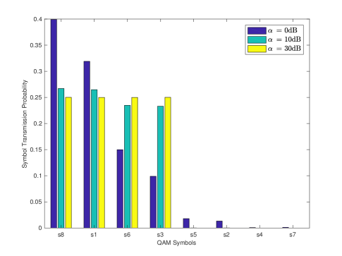
Figure 1: $8$-QAM probability distribution for three SNR levels at $\eta=0.99$ and Rate = $2$ bits/symbol.

IV-C Toy Examples

A comprehensive illustration of probabilistically shaped $M_{\rm nu}=8$-QAM with a $2$ bits/symbol rate constraint, corresponding to $M_{\rm u}=4$, is presented in Fig. 1 and Fig. 2. The relation between prior probabilities and different SNR values is presented in Fig. 1. Clearly, the probability distribution is quite random for lower SNR level such as $\alpha=0$ dB. However, it starts adopting uniform distribution of $0.25$ for four of it’s symbols, i.e., s1, s3, s6, and s8 while zero probabilities for the rest four symbols. This technique provides lower BER while maintaining $2$ bits/symbol rate for a fair comparison with traditional $4$-QAM. Interestingly, it achieves a lower BER by transmitting half of the symbols which are not the nearest neighbors. It is important to highlight that the proposed approach achieves this performance with the same power budget and transmission rate.

Another example illustrates the trend of probabilitic shaping for $8$-QAM constellation at lower SNR level (keeping in mind that it assigns the uniform probabilities to four symbols at high SNR levels). The trend for lower HWD level such as $\eta=0.11$ is quite random. However, it follows a decreasing probability trend for middle to higher HWD levels. Intuitively, it assigns higher probabilities to the symbols with least power and lower probabilities to the symbols with higher powers. This trend decreases the BER while maintaining the average power constraint.

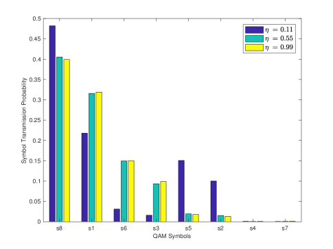
Figure 2: $8$-QAM probability distribution for three HWD levels at $\alpha=0$ dB and Rate = $2$ bits/symbol.

V Hybrid Shaping where Conventional meets State-of -the-Art

In this section, we increase the AS design flexibility by allowing joint GS and PS, which we call it here HS, to improve the underlying communication system performance further. Throughout the design procedure, HS transforms the equally spaced uniformly distributed QAM/PSK symbols to unequally spaced symbols in a geometric envelope with non-uniform prior distribution. Thus, HS aims to optimize the symbol probabilities (i.e., PS) and some spatial shaping parameters for the constellation (i.e., GS).

V-A Hybrid Shaping Parameterization

Apart from the non-uniform priors, consider the asymmetric transmit symbol ${\bf v}_{m}=\left[{v}_{mI}\quad{v}_{mQ}\right]^{\rm T}$ resulting from the GS on the conventional baseband symmetric $M$-QAM/$M$-PSK symbol ${\bf x}_{m}=\left[{x}_{mI}\quad{x}_{mQ}\right]^{\rm T}$ as $\mathbf{v}_{m}=\mathbf{AR}\mathbf{x}_{m}$, where

$${\bf{A}}\left(\zeta\right)=\left[{\begin{array}[]{*{20}{c}}{\sqrt{1+\zeta}}&{0}\\ {0}&{\sqrt{1-\zeta}}\end{array}}\right],$$ (34)

with translation parameter $\zeta\in\left(0,1\right)$. Furthermore, the rotation is given by

$${\bf{R}}\left(\theta\right)=\left[{\begin{array}[]{*{20}{c}}{\cos\left(\theta\right)}&{-\sin\left(\theta\right)}\\ {\sin\left(\theta\right)}&\quad{\cos\left(\theta\right)}\end{array}}\right],$$ (35)

with rotation angle $\theta\in\left(0,\mu\,\pi/2\right)$ for some constant $\mu$. Uniformly distributed symmetric $M$-QAM constellation has a rotation symmetry of $n\,\pi/2,n\in\mathcal{Z}^{+}$ rendering $\mu=n$ to be good choice for GS. However, non-uniformly distributed $M$-QAM constellation can only be rotationally symmetric after $2n\pi$, thus $\mu=4n$ is suitable for HS. This technique renders non-uniformly spaced symbols in a parallelogram envelop. It is important to highlight that this transformation preserves the power requirement. Power invariance of the rotation is a well known fact in the literature [66]. However, the wisdom behind the structure of $\mathbf{A}\left(\zeta\right)$ is unfolded in the following theorem.

Remark 1.

GS parameterization using translation matrix ${\mathbf{A}}\left(\zeta\right)$ preserves the power invariance of a complex random variable and inculcates asymmetry/improperness with the circularity coefficient $\zeta$.

Proof.

The proof is presented in Appendix B. Furthermore, the generalization of the same concept to the symmetric discrete constellations such as $M$-QAM and $M$-PSK is also described in Appendix B. ∎

V-B Optimal Receiver

The optimal receiver for hybrid shaped AS is also a MAP detector as derived in (9), but with a modified reference constellation $v_{m}$ in place of $x_{m}$ for all $m\in\{1,2,\cdots,M_{\rm nu}\}$. More precisely, the detected symbol, $\hat{m}_{\rm HS}$, is the one that maximizes the posterior distribution, i.e.,

$$\hat{m}_{\rm HS}=\mathop{\arg\max}\limits_{1\leq m\leq M_{\rm nu}}\quad p_{V}(v_{m}){f_{{Y_{\rm I}},{Y_{\rm Q}}|V,g}}\left({{y_{\rm I}},{y_{\rm Q}}|{v_{m}},g}\right),$$ (36)

where, ${f_{{Y_{\rm I}},{Y_{\rm Q}}|V,g}}\left({{y_{\rm I}},{y_{\rm Q}}|{v_{m}},g}\right)$ is similar to (10) by replacing all appearances if $x_{m}$ with $v_{m}$ for all $m\in\{1,2,\cdots,M_{\rm nu}\}$. It is worth noting that non-uniform prior probabilities are inculcated in the detection process using MAP detector in place of ML detector. Moreover, the geometrically shaped symbols are taken from a modified symbol constellation. Hence, this requires updating the reference constellation for appropriate detection.

V-C Error Probability

HS follows the same BER bound as derived in (22) but with modified $\gamma_{mn}$. It can now be written using the following quadratic formulation as a function of $\zeta$ and $\theta$.

$$\gamma_{mn}\left(\zeta,\theta\right)={\bf{x}}_{mn}^{\rm T}{{\bf R}\left(\theta\right)}^{\rm T}{{\bf A}\left(\zeta\right)}^{\rm T}{\bf G}{\bf A}\left(\zeta\right){\bf R}\left(\theta\right){\bf{x}}_{mn},$$ (37)

where ${\mathbf{x}}_{mn}$ is the real composite vector form of $\xi_{mn}=gd_{mn}$ given by

$${\mathbf{x}}_{mn}=\left[{\xi_{mn}}_{\rm I}\quad{\xi_{mn}}_{\rm Q}\right]^{T},$$ (38)

and ${\mathbf{G}}$ contains the statistical characteristics of the aggregate noise including in-phase noise variance, quadrature-phase noise variance, and the correlation between these components.

$${\mathbf{G}}=\left[{\begin{array}[]{*{20}{c}}\frac{1}{\sigma_{I}^{2}}&\frac{-\rho_{z}}{\sigma_{I}\sigma_{Q}}\\ \frac{-\rho_{z}}{\sigma_{I}\sigma_{Q}}&\frac{1}{\sigma_{Q}^{2}}\end{array}}\right].$$ (39)

Thus, the BER of HS can be upper bounded as

$${{\rm{P}}_{\rm b,HS}^{\rm UB}}\left({\mathbf{p}},\zeta,\theta\right)=\frac{1}{{{{\log}_{2}}\left(M_{\rm nu}\right)}}\sum\limits_{m=1}^{M_{\rm nu}}{\sum\limits_{{n=1}\atop{n\neq m}}^{M_{\rm nu}}{{p_{m}}}}\\ \times\mathcal{Q}\left(\frac{\sqrt{1-{\rho_{z}^{2}}}}{\sqrt{\alpha\gamma_{mn}\left(\zeta,\theta\right)}}\ln\left({\frac{{{p_{m}}}}{{{p_{n}}}}}\right)+\frac{\sqrt{\alpha\gamma_{mn}\left(\zeta,\theta\right)}}{2\sqrt{1-{\rho_{z}^{2}}}}\right).$$ (40)

V-D Problem Formulation

HS targets the joint design of PS PMF ${\mathbf{p}}$ and GS parameters involving translation $\zeta$ and rotation $\theta$ parameter to minimize the BER bound given in (40).

$$\textbf{P2}:\quad \!\!\!\!\underset{{{{\bf p}\in\mathbb{S},}{0\leq\zeta\leq 1,}}\atop{0\leq\theta\leq 2{\pi}}}{\text{minimize }} {{\rm{P}}_{\rm b,HS}^{\rm UB}}\left({\mathbf{p},\zeta,\theta}\right)$$ (41a)

subject to $$\sum\limits_{m=1}^{M_{\rm nu}}{{{\left|{{v_{m}}}\right|}^{2}}{p_{m}}\leq 1},$$ (41b)

$${\rm H}({\mathbf{p}})\geq\log_{2}\left({M_{\rm u}}\right),$$ (41c)

where the average power constraint (25b) is updated as (41b) to account for the possible change in the power of the symbols by geometrically shaping the constellation. However, the proposed rate constraint (41c) remains intact. Additionally, there are some boundary constraints on $\zeta$ and $\theta$, respectively.

Intuitively, it is quite difficult to tackle this non-convex multimodal joint optimization problem. Therefore, we resort to the alternate optimization of PS parameters (${\mathbf{p}}$) and GS parameters ($\zeta,\theta$) using sub-problems P2a and P2b, respectively. Problem P2a designs the PS parameters for some given $\zeta$ and $\theta$. It is quite similar to the problem P1 and thus, can be solved using Algorithm 1.

$$\textbf{P2a}:\quad \!\!\!\!\underset{{{\bf p}\in\mathbb{S}}}{\text{minimize }} \!\!\!\!{{\rm{P}}_{\rm b,HS}^{\rm UB}}\left({\mathbf{p},\zeta,\theta}\right)$$ (42)

subject to $$\!\!\!\!\eqref{eq.2pc},\eqref{eq.2rc}.$$

On the other hand, the GS optimization problem designs $\zeta$ and $\theta$ for fixed symbol probabilities $\bf{p}$, given as

$$\textbf{P2b}:\quad \!\!\!\!\underset{{0\leq\zeta\leq 1,}\atop{0\leq\theta\leq 2{\pi}}}{\text{minimize }}{{\rm{P}}_{\rm b,HS}^{\rm UB}}\left({\mathbf{p}},\zeta,\theta\right).$$ (43)

The optimization problem P2b is a multimodal non-convex problem which is hard to tackled even by the SCP approach as employed in Section IV. The difficulty arises due to the absence of any constraints which restrict the feasibility region. The feasibility space enclosed by the boundary constraints is highly insufficient to serve our purpose. Therefore, we can approximate the solution using any of the following two methods

• Trust region reflective method: This method defines a trust region around a specific initial point and then approximate the function within that region. The convex approximation is the first order Taylor series approximation using the gradient. It begins by minimizing convex approximation of the function to obtain a solution. This solution is the perturbation in the initial point rendering a new point which should minimize the original function. Otherwise, we need to shrunk the trust region and repeat the process. Reflections are used to increase the step size while satisfying box constraints. After each iteration, we receive a new point which renders a lower objective function than the initial point. This iterative approach leads us to a local minimum and stops when some specified stopping criterion are met [68, 69].

• Gradient descent: This method is a relatively faster approach to tackle the problem at hand. It is owing to the fact that it does not involve any approximation and underlying optimization. It begins with an initial point and keeps updating the point in the descent direction using the gradients and a step size until it reaches a local solution or satisfies some stopping criterion [67].

Interestingly, both of these methods require the gradients of ${{\rm{P}}_{\rm b,HS}^{\rm UB}}\left({\mathbf{p}},\zeta,\theta\right)$ with respect to $\zeta$ and $\theta$. Gradients are used either to approximate the function with it’s first order Taylor series approximation within a trust region or to find the next point in the descent direction. The gradients are evaluated and presented in Appendix D.

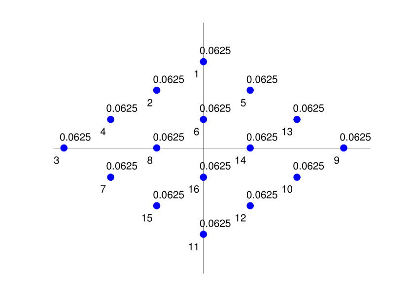
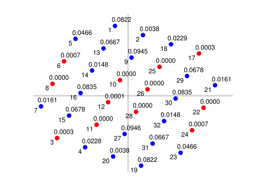
Figure 3: Different Asymmetric Signaling Designs

(a) No Shaping                 (b) Geometric Shaping
  
(c) Probabilistic Shaping                (d) Hybrid Shaping

V-E Proposed Algorithm

The joint optimization problem P2 can be tackled using the alternate optimization algorithm as presented in Algorithm 2. It solves the sub problems P2a and P2b alternately and iteratively. It begins with some starting feasible points ${\mathbf{p}}^{(j)}$, $\zeta^{(j)}$, and $\theta^{(j)}$ and evaluates ${{\rm{P}}_{\rm b,HS}^{{\rm UB}{(j)}}}\left({\mathbf{p}}^{(j)},\zeta^{(j)},\theta^{(j)}\right)$ as a benchmark. The alternate optimization begins by solving P2a to minimize ${\rm{P}}_{\rm b,HS}^{\rm UB}$ with respect to ${\mathbf{p}}$ given a pair of $\zeta$ and $\theta$. It is achieved by replacing all entries of $x_{m}$ with $v_{m}={\bf AR}x_{m}\;\forall m$. ${\mathbf{p}}^{(j*)}$ is obtained using the framework provided in Algorithm 1 which solves P1a iteratively. Then, the optimum ${\mathbf{p}}^{(j*)}$ is used as a given PMF to obtain the pair $\zeta^{(j*)}$ and $\theta^{(j*)}$ by solving P2b. These optimum parameter values are updated to attain next initial points. Moreover, ${{\rm{P}}_{\rm b,HS}^{{\rm UB}{(j+1)}}}\left({\mathbf{p}}^{(j+1)},\zeta^{(j+1)},\theta^{(j+1)}\right)$ is also evaluated to compare the decrease in objective function. The norm of this difference is stored in $\epsilon$ and the process is repeated until this value drops below a preset threshold $\delta$. Eventually, the solution parameters are updated in $\left({\mathbf{p}}^{*},\zeta^{*},\theta^{*}\right)$ which yield the minimized BER upper bound ${\rm{P}}_{\rm b,HS}^{{\rm UB}*}$ using HS. Therefore, these HS parameters are capable of rendering a BER ${\rm{P}}_{\rm b,HS}^{*}$ lower than the bound ${\rm{P}}_{\rm b,HS}^{{\rm UB}*}$.

Algorithm 2 Alternate Optimization

1:Initialize $j\leftarrow 0$, $\epsilon\leftarrow\infty$ and Set tolerance $\delta$

2:Choose feasible starting points ${\mathbf{p}}^{(j)}$, $\zeta^{(j)}$, and $\theta^{(j)}$.

3:Evaluate ${{\rm{P}}_{\rm b,HS}^{{\rm UB}{(j)}}}\left({\mathbf{p}}^{(j)},\zeta^{(j)},\theta^{(j)}\right)$.

4:while $\epsilon\geq\delta$ do

5:     Solve P2a using Algorithm 1 with starting point ${\mathbf{p}}^{(j)}$ and given $\zeta^{(j)}$, $\theta^{(j)}$ to obtain ${\mathbf{p}}^{(j*)}$

6:     Solve P2b with starting points $\zeta^{(j)}$,$\theta^{(j)}$ and given ${\mathbf{p}}^{(j*)}$ to obtain $\zeta^{(j*)}$, $\theta^{(j*)}$

7:     ${{\mathbf{p}}}^{(j+1)}\leftarrow{\mathbf{p}}^{(j*)}$, $\zeta^{(j+1)}\leftarrow\zeta^{(j*)}$, and $\theta^{(j+1)}\leftarrow\theta^{(j*)}$

8:     Evaluate ${{\rm{P}}_{\rm b,HS}^{{\rm UB}{(j+1)}}}\left({\mathbf{p}}^{(j+1)},\zeta^{(j+1)},\theta^{(j+1)}\right)$.

9:     Update ${\epsilon\leftarrow\left\|{{\rm{P}}_{\rm b,HS}^{{\rm UB}{(j+1)}}}-{{\rm{P}}_{\rm b,HS}^{{\rm UB}{(j)}}}\right\|}$

10:     ${j\leftarrow j+1}$

11:end while

12:Solution parameters: ${\mathbf{p}}^{*}\leftarrow{\mathbf{p}}^{j+1}$, $\zeta^{*}\leftarrow\zeta^{j+1}$, $\theta^{*}\leftarrow\theta^{j+1}$

13:Objective function: ${{\rm{P}}_{\rm b,HS}^{{\rm UB}{*}}}\leftarrow{{\rm{P}}_{\rm b,HS}^{{\rm UB}{(j+1)}}}$

14:Consequence: $\rm{P}_{\rm b,HS}^{*}\leq{{\rm{P}}_{\rm b,HS}^{{\rm UB}{*}}}$

Numerical evaluations reveal that the stopping criteria is mostly met in just one iteration. Interestingly, Step 5 and 6 in Algorithm 2 are interchangeable and need to be chosen carefully. For instance, PS demonstrates better performance at higher HWD levels so it is intuitive to design the HS by first PS and then GS in order to attain further gain over PS. Whereas, GS depicts lower BER at lower HWD levels so it is recommended to design HS by first GS and then PS in order to achieve better performance than GS using the added DoF offered by PS.

HS can be implemented by choosing the transmit symbols for the translated and rotated signal constellation, i.e., $v_{m}=\mathbf{A}\left(\zeta^{*}\right)\mathbf{R}\left(\theta^{*}\right)x_{m}$. Furthermore, the symbols are transmitted according to the optimized ${\mathbf{p}}^{*}$ where $\zeta^{*}$, $\theta^{*}$ and ${\mathbf{p}}^{*}$ are designed using Algorithm 2. Upon reception, they are detected using the MAP detector as presented in (36).

V-F Illustrative Example

We present a comprehensive example to highlight the design of various distinct shapes for a fixed rate of 4bits/symbol. The black color is used for the reference constellation. The blue color depicts the possible transmission symbols whereas red symbols highlight the improbable transmission symbols. Fig. 3a presents uniformly distributed $16$-QAM constellation with no-shaping. Fig. 3b illustrates geometrically shaped $16$-QAM with parameters $\zeta=0.5$ and $\theta=\pi/2$. The parallelogram envelop encloses equally prior QAM symbols. Next, we employ $32$-QAM and design non-uniform probabilities as detailed in section IV. The red symbols highlight the symbols with negligible transmission probabilities whereas blue symbols have some notable transmission probabilities as depicted in Fig. 3c. The proposed algorithm tends to discard symbols with minimal transmission power to reduce the BER. One possible reason is that these symbols are mostly affected by the improper HWD owing to their comparable power/variance. Furthermore, this probabilistic shaped constellation undergoes GS to demonstrate hybrid shaped QAM constellation as shown in Fig. 3d.

VI Numerical Results

Numerical evaluations of the adopted HWD system are carried out to study the drastic effects of hardware imperfections and the effectiveness of the mitigation strategies. The performance of the proposed PS and HS as a realization of asymmetric transmission is quantified with varying energy per bit per noise ratio (EbNo) and HWD levels. EbNo is obtained by normalizing SNR with the transmission rate. The derived error probability bounds and performance of the asymmetric transmission schemes are also validated using Monte-Carlo simulations. We compare the performance of conventional GS with the proposed PS. GS can be implemented by transmitting symbols from a reshaped constellation $\mathbf{v}_{m}=\mathbf{A}\left(\zeta^{*}\right)\mathbf{R}\left(\theta^{*}\right)\mathbf{x}_{m}$, where $\zeta^{*}$ and $\theta^{*}$ can be obtained by solving P2a given uniform prior distribution. Upon reception, they are detected using the ML detector which is the simplified form of optimal MAP detector (36) given uniform prior probabilities. This ML detector considers the reshaped constellation symbols $\mathbf{v}_{m}$ as the reference to detect the received symbols.

For most of the numerical evaluations we assume grey coded square QAM constellations of order $M_{\rm u}=8$, i.e., $R=\log_{2}(M_{\rm u})$, for no-shaping (NS) and GS as benchmarks. For PS and HS we employ $M_{\rm nu}=32$-QAM with rate at least as high as that of GS, i.e., $R\geq\log_{2}(M_{\rm u})$. Moreover, we consider practical HWD values for the transmitter $\kappa_{t}=0.01$ and receiver $\kappa_{r}=0.12$. The pseudo-variances are derived from the $\tilde{\kappa}_{\rm tI}=\kappa_{t}/4$, $\tilde{\kappa}_{\rm rI}=\kappa_{r}/4$, and correlation coefficient $\rho_{\eta}=0.9$. Intuitively, AWGN channel assumes $g=1$ and circularly symmetric Rayleigh fading channel is generated using $\lambda=1$. Furthermore, the transmission EbNo is taken as $30$ dB. The aforementioned values of the parameters are used throughout the numerical results, unless specified otherwise.

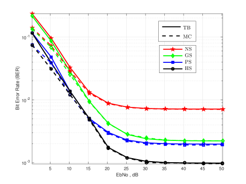
Figure 4: BER performance for a range of EbNo with $\kappa=0.13$ in AWGN channel.

First, we evaluate the performance of various AS schemes for a range of EbNo from $0$ dB to $50$ dB in an AWGN channel as shown in Fig. 4. We employ $M_{\rm u}$-QAM for NS and GS whereas $M_{\rm nu}$-QAM for PS and HS. The BER performance improves with increasing EbNo till $30$ dB and then undergoes saturation owing to the presence of HWD. Further increase in bit energy also results in an increase in the distortion variance, as the system experiences an error floor which can be deduced from (24). Evidently, the proper/symmetric QAM is suboptimal and the BER performance is significantly improved using AS. Conventional GS is not beneficial at lower EbNo values, but it significantly improves the performance for higher EbNo values pertaining to the increased symbol space [36]. On the other hand, the proposed PS is capable of minimizing the BER for the entire range of EbNo. Substantial gains can be achieved by taking another step forward and employing HS. Therefore, we can safely conclude that the best performance can be achieved using PS for EbNo $\leq$ $15$ dB and HS for EbNo $\geq$ $15$ dB as validated by the Monte Carlo simulation. At $20$ dB, the BER reductions for GS, PS, and HS schemes with respect to unshaped constellation are approximately $52.22$%, $66.67$%, $80$%, respectively.

For the same simulation settings, we analyze system throughput (correct bits/symbol) for a range of EbNo values where the lower bound on system throughput can be obtained as

$$\mathcal{T}^{\rm LB}\left(\mathbf{p}\right)=\left[1-{{\rm{P}}_{b}^{\rm UB}}\left(\mathbf{p}\right)\right]{\rm{H}}(\mathbf{p})$$ (44)

Fig. 5 depicts negligible throughput gain of GS over NS but noticeable throughput improvement using PS or HS. For instance, $1.5$%, $6$% and $7$% percentage increase in throughput can be observed using GS, PS, and HS at $\text{EbNo}=5$ dB. The throughput gain is quite substantial for lower EbNo values but undergoes saturation when EbNo $\geq$ $20$ dB. Interestingly, PS/HS saturates at $3$ bits/symbol following rate fairness constraint with negligible BER whereas other schemes saturate below $3$ bits/symbol depicting significant BER even though the entropy of $8$-QAM with uniform distribution is $\log_{2}(8)=3$.

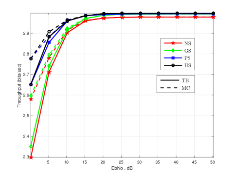
Figure 5: Throughput performance for a range of EbNo with $\kappa=0.13$ in AWGN channel.

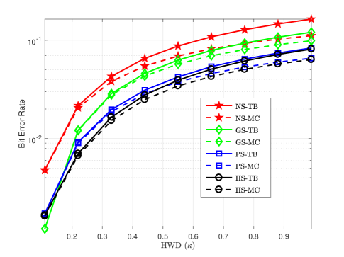
Figure 6: HWD mitigation using $16$-QAM for PS and HS at $\text{EbNo}=30$ dB in an AWGN channel.

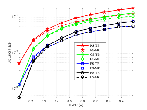
Figure 7: HWD mitigation using $32$-QAM for PS and HS at $\text{EbNo}=30$ dB in an AWGN channel.

Next we analyze the behavior of various AS schemes with increasing distortion levels as depicted in Fig. 6. We assume $8$-QAM for benchmark NS and traditional GS whereas $16$-QAM for PS and HS. Derived bounds are in close accordance with the MC simulation especially for lower HWD levels. Obviously, the BER increases with increasing HWD levels and AS based systems achieve lower BER by efficiently mitigating the drastic HWD effects. Undoubtedly, the NS scheme suffers the most, but GS helps to decrease the BER to some extent. Further compensation can be achieved using the proposed PS and HS. Surprisingly, GS outperforms PS and HS at the lowest HWD values, e.g., $\kappa=0.11$, in Fig. 6 but PS/HS maintain their superiority for $\kappa\geq 0.17$. Interestingly, PS/HS are still capable of outperforming GS even for the lowest HWD levels pertaining to their rate adaptation capability and added DoF using $32$-QAM as highlighted in Fig. 7. We can observe enhanced mitigation offered by the $32$-QAM PS/HS as compared to the $16$-QAM PS/HS due to the added DoF. For instance, we observe BER compensation of $66$% and $77.5$% using $32$-QAM PS and HS, respectively, whereas BER compensation of $55$% and $65$% using $16$-QAM PS and HS, respectively, at $\kappa=0.22$ HWD level.

A similar analysis is undertaken to study the impact of increasing HWD on the system throughput. Fig. 8 compares the throughput performance of $M_{\rm u}$-QAM NS and GS with $M_{\rm nu1}=16$-QAM PS and HS as well as with $M_{\rm nu2}=32$-QAM PS and HS. System throughput decreases almost linearly with increasing HWD for all forms of signaling but with different slopes. NS demonstrates the steepest slope with increasing HWD and all the other AS schemes render gradual slopes. Quantitative analysis shows the slopes of $-0.55$, $-0.41$, $-0.28$, and $-0.24$ using NS, GS, $16$-QAM PS/HS, and $32$-QAM PS/HS, respectively, with increasing HWD. Therefore, PS and HS present the most favorable results as compared to the GS. Their performance can be even improved by increasing the modulation order. Another important observation is the overlapping response of PS and HS especially for higher ordered QAM, which suffices PS and revokes the need of HS to perform even better.

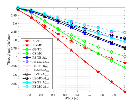
Figure 8: System throughput for a range of HWD levels at $\text{EbNo}=30$ dB in an AWGN channel.

Another simulation example depicts the performance of the discussed AS schemes with over a range of EbNo for two distinct scenarios of perfect receiver and perfect transmitter as presented in Fig. 9. Perfect receiver system as the name specifies includes ideal zero-distortion receiver but imperfect transmitter with $\kappa_{t}=0.07$ whereas perfect transmitter system involves ideal zero-distortion transmitter but imperfect receiver with $\kappa_{r}=0.15$. Note that the lower value of $\kappa_{t}$ relative to $\kappa_{r}$ is due to the fact that transmitters employ sensitive equipment to exhibit low distortions because the transmitter distortions are far more drastic than the receiver distortions. Interestingly, GS outperforms PS at EbNo > $15$ dB for the perfect receiver case as opposed to EbNo < $15$ dB where PS is still a better choice. HS outperforms both of them irrespective of the EbNo range classification. At such low HWD level, the BER percentage reduction of $81.82$%, $90.91$%, $94.55$% is observed using PS, GS, and HS at $30$ dB EbNo. Regarding the perfect transmitter scenario, GS and PS reverse the trend for higher EbNo level. Now the PS clearly outperforms GS for the entire range of EbNo and the HS marks its superiority over both of these schemes. At $0.15$ HWD level, the EbNo gain of $8$ dB, $12$ dB, and $13$ dB are estimated using GS, PS, and HS to attain the BER of $10^{-2}$.

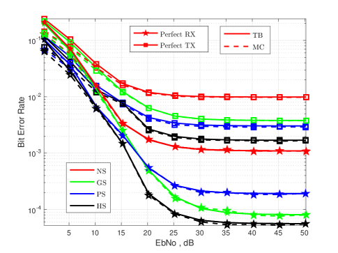
Figure 9: BER performance for two different HWD scenarios (Perfect Receiver: $\kappa_{t}=0.07$ and Perfect Transmitter: $\kappa_{r}=0.15$) in an AWGN channel.

Finally, the average (ergodic) BER performance of the adopted system with $\kappa=0.22$ HWD level is evaluated over a Rayleigh fading channel for a range of EbNo values as given in Fig. 10. Evidently, the AS schemes preserve their BER trends and order. Clearly, average BER decreases with increasing EbNo and then undergoes saturation yielding an error floor. The derived BER bounds are also validated using MC simulations rendering a tighter bound for higher EbNo values. GS improves the average BER as compared to the NS scenario but PS and HS maintain their superior performance. Signaling schemes of GS, PS, and HS offer a percentage reduction of $54.55$%, $63.64$%, and $70.45$%, respectively, in the average BER performance at $40$ dB EbNo.

In a nutshell, we can conclude that the GS offers significant BER reduction at higher SNR values as opposed to the PS which offers universal gains. Moreover, the perks of HS are also prominent for higher SNR and higher $M$-ary modulation but depicts PS comparable performance at lower SNR values. Therefore, we recommend to employ HS given high SNR but resort to PS for lower SNR values to save additional computational expense. Additionally, GS is a better choice for slightly distorted systems whereas PS/HS are the optimal choice for moderate to severely distorted systems. Furthermore, we can achieve improved performance by employing higher-order QAM constellations for PS/HS given adequate resources. On the other hand, the throughput gains are eminent at considerably lower SNR values and higher distortion values.

Table I: First Order Necessary KKT Conditions

Index	KKT Conditions	Satisfied with	Reason
$1:M_{\rm nu}$	$\nabla_{\mathbf{p}}\mathcal{L}\left({\mathbf{p}}^{*},{\lambda^{*}}\right)=0,\;\forall 1\leq m\leq M_{\rm nu}$	$\nabla_{\mathbf{p}}\mathcal{L}\left({\mathbf{p}}^{*},{\lambda_{1}^{*}},{\lambda_{2}^{*},{\lambda_{3}^{*}}}\right)=0$	Saddle point of the dual problem
$M_{\rm nu}$+1	${\lambda_{1}^{*}}\left({\sum\limits_{m=1}^{M_{\rm nu}}{{\left|{{x_{m}}}\right|}^{2}}{p_{m}^{*}}-1}\right)=0$	${\sum\limits_{m=1}^{M_{\rm nu}}{{\left|{{x_{m}}}\right|}^{2}}{p_{m}^{*}}}=1$, ${\lambda_{1}^{*}}\geq 0$	Maximum power transmission
$M_{\rm nu}$+2	${\lambda_{2}^{*}}\left({\sum\limits_{m=1}^{M_{\rm nu}}{p_{m}^{*}}-1}\right)=0$	${\sum\limits_{m=1}^{M_{\rm nu}}{p_{m}^{*}}}=1$, ${\lambda_{2}^{*}}\geq 0$	Equality constraint
$M_{\rm nu}$+3	${\lambda_{3}^{*}}\left(\log_{2}\left({M_{\rm u}}\right)-{\rm H}({\mathbf{p}}^{*})\right)=0$	${\rm H}({\mathbf{p}}^{*})=\log_{2}\left({M_{\rm u}}\right)$, ${\lambda_{3}^{*}}\geq 0$	BER -Rate tradeoff

VII Conclusion

This work proposes probabilistic and hybrid shaping to realize asymmetric signaling in digital wireless communication systems suffering from improper HWD. Instinctively, all forms of asymmetric shaping are capable of decreasing the BER, and this performance gain improves with increasing SNR and/or increasing HWD levels with respect to NS. However, PS outperforms GS and performs equally well as HS. We can achieve more than $50$% BER reduction with PS/HS over traditional GS. The perks of PS come at the cost of increased complexity in the design and decoding process. The HS scheme is capable of improving the system performance in terms of the BER as well as throughput. However, for less HWD levels and low EbNo, the benefits of HS over PS are limited while requiring additional complications in optimization, modulation, and detection procedures. Therefore, PS emerges as the best choice in the trade-off between enhanced performance and added complexity.

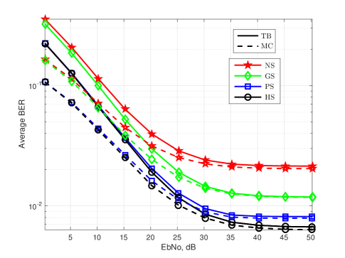
Figure 10: Average BER performance with HWD $\kappa=0.22$ in a Rayleigh fading channel.

Appendix A Statistical Characterization of Aggregate Noise

The superposed Gaussian distributions render the accumulative noise $z\sim\mathcal{CN}\left({0,v,\tilde{v}}\right)$, where $v=\alpha{{\left|g\right|}^{2}}\kappa+\sigma_{w}^{2}$ and ${\tilde{v}}=\alpha{g^{2}}\tilde{\kappa}$. Exploiting the relation between the $v$, $\tilde{v}$ and the variances of $\sigma_{I}^{2}=E\{z_{I}^{2}\}$, $\sigma_{Q}^{2}=E\{z_{Q}^{2}\}$ and their mutual correlation ${r_{{z_{I}}{z_{Q}}}}=E\left\{{{z_{I}}{z_{Q}}}\right\}$, we get

$$v={E\left\{{{{\left|z\right|}^{2}}}\right\}=\sigma_{I}^{2}+\sigma_{Q}^{2}}.$$ (45)

$${\tilde{v}}=E\left\{{{z^{2}}}\right\}=\sigma_{I}^{2}-\sigma_{Q}^{2}+i2{r_{{z_{I}}{z_{Q}}}}.$$ (46)

Their inter relation enables us to evaluate $\sigma_{I}^{2}$, $\sigma_{Q}^{2}$, and ${r_{{z_{I}}{z_{Q}}}}$ from $v$ and $\tilde{v}$ as

$${\sigma_{I}^{2}=\frac{{v+{{\tilde{v}}_{I}}}}{2}=\frac{{\alpha{{\left|g\right|}^{2}}\kappa+\sigma_{w}^{2}+\alpha{\Re}\left({{g^{2}}\tilde{\kappa}}\right)}}{2}},$$ (47)

$${\sigma_{Q}^{2}=\frac{{v-{{\tilde{v}}_{I}}}}{2}=\frac{{\alpha{{\left|g\right|}^{2}}\kappa+\sigma_{w}^{2}-\alpha{\Re}\left({{g^{2}}\tilde{\kappa}}\right)}}{2}},$$ (48)

$${r_{{z_{I}}{z_{Q}}}}=\frac{{{{\tilde{v}}_{Q}}}}{2}=\frac{{\alpha{{\Im}}\left({{g^{2}}\tilde{\kappa}}\right)}}{2}.$$ (49)

Finally, (47)-(49) allow us to find the correlation coefficient between $z_{I}$ and $z_{Q}$ as

$$\rho_{z}=\frac{{{r_{{z_{I}}{z_{Q}}}}}}{{{\sigma_{I}}{\sigma_{Q}}}}={\frac{{\alpha{\Im}\left({{g^{2}}\tilde{\kappa}}\right)}}{{\sqrt{{{\left({\alpha{{\left|g\right|}^{2}}\kappa+\sigma_{w}^{2}}\right)}^{2}}-{{\left({\alpha{\Re}\left({{g^{2}}\tilde{\kappa}}\right)}\right)}^{2}}}}}}.$$ (50)

Appendix B Translation within power budget

In this appendix we present the proof of Remark 1. It is straightforward to prove that the translation $\mathbf{v}=\mathbf{A}\mathbf{w}$ does not change the variance/power but only introduce asymmetry/improperness. Considering the transformation caused by the translation ${v}=\sqrt{1+\zeta}w_{I}+i\sqrt{1-\zeta}w_{Q}$, the power/variance is given by

$$\sigma_{v}^{2}=({1+\zeta})\sigma_{w_{I}}^{2}+({1-\zeta})\sigma_{w_{Q}}^{2}.$$ (51)

Using the symmetric nature of r.v. $w$ i.e., $\sigma_{w_{I}}^{2}=\sigma_{w_{Q}}^{2}$, it is clear that $\sigma_{v}^{2}=\sigma_{w}^{2}$. On the other hand, the pseudo-variance can be calculated as

$$\tilde{\sigma}_{v}^{2}=({1+\zeta})\sigma_{w_{I}}^{2}-({1-\zeta})\sigma_{w_{Q}}^{2}+i2\sqrt{1-\zeta^{2}}{E\left\{w_{I}w_{Q}\right\}}.$$ (52)

Again, the symmetry implies ${E\left\{w_{I}w_{Q}\right\}}=0$. Thus, the circularity coefficient can be derived from (52) i.e., ${|\tilde{\sigma}_{v}^{2}|}/{\sigma_{v}^{2}}=\zeta$.

The same concept can be extended to the symmetric discrete constellations with uniform prior probabilities. Considering the transformation caused by the translation $v_{m}=\sqrt{1+\zeta}x_{mI}+i\sqrt{1-\zeta}x_{mQ}$, the power of the transformed constellation is given by

$$P=\frac{1}{M}\left(({1+\zeta})\sum\limits_{m=1}^{M}x_{mI}^{2}+({1-\zeta})\sum\limits_{m=1}^{M}x_{mQ}^{2}\right).$$ (53)

Using the symmetric property of the original discrete constellation $\sum\limits_{m=1}^{M}x_{mI}^{2}=\sum\limits_{m=1}^{M}x_{mQ}^{2}$, it is clear that the power is preserved as $P=\frac{2}{M}\sum\limits_{m=1}^{M}x_{mI}^{2}$. Moreover, the non-zero pseudo-variance is given by

$$\tilde{P}=\zeta P+\frac{2i}{M}\sqrt{1-\zeta^{2}}\sum\limits_{m=1}^{M}x_{mI}\,x_{mQ}.$$ (54)

Again, the symmetry implies $\sum\limits_{m=1}^{M}x_{mI}x_{mQ}=0$. Thus, the circularity coefficient can be derived from (54), i.e., ${{|\tilde{P}|}/{P}=\zeta}$.

Appendix C KKT Conditions

The convex non-linear constraint problem P1a can be efficiently solved using the first order necessary KKT conditions. We begin by writing the Lagrangian function $\mathcal{L}$ as

$$\mathcal{L} \left({\mathbf{p}},{\lambda_{1}},{\lambda_{2}},{\lambda_{3}}\right)=\!{\tilde{\rm{P}}_{\rm b}^{\rm UB}}\!\left(\!{\mathbf{p}},{\mathbf{p}}^{(k)}\right)\!+\!{\lambda_{1}}\!\left(\!{\sum\limits_{m=1}^{M}{{\left|{{x_{m}}}\right|}^{2}}{p_{m}}\!-\!1\!}\right)$$

$$\qquad\quad+\!{\lambda_{2}}\!\left({\sum\limits_{m=1}^{M}{p_{m}}\!-\!1}\right)\!+\!{\lambda_{3}}\!\left(\log_{2}\left({M_{\rm u}}\right)\!-\!{\rm H}({\mathbf{p}})\right),$$ (55)

where the Lagrange multipliers are ${\lambda_{1}},{\lambda_{2}}$, ${\lambda_{3}}\geq 0$. Next. we evaluate the gradient of the (C) with respect to the optimization variables in ${\mathbf{p}}$

$$\nabla_{{\mathbf{p}}}{\mathcal{L}}=\left[\frac{{\partial\mathcal{L}}}{{\partial{p_{1}}}}\quad\frac{{\partial\mathcal{L}}}{{\partial{p_{2}}}}\quad\ldots\quad\frac{{\partial\mathcal{L}}}{{\partial{p_{M_{\rm nu}}}}}\right],$$ (56)

where the partial derivative of ${\mathcal{L}}$ with respect to ${p_{m}}$ is given by

$$\frac{{\partial\mathcal{L}}}{{\partial{p_{m}}}}= \frac{{\partial{{\rm{P}}_{\rm b}^{\rm UB}}\left({\mathbf{p}}^{(k)}\right)}}{{\partial{p_{m}}}}+{\lambda_{1}}{\left|{{x_{m}}}\right|^{2}}+{\lambda_{2}}$$

$$+{\lambda_{3}}\left({\frac{1}{{\ln(2)}}\!+\!{{\log}_{2}}\left({{p_{m}}}\right)}\right),\quad\forall\,1\leq m\leq M_{\rm nu}$$ (57)

Suppose that there is a local solution ${\mathbf{p}}^{*}$ of P1a and the objective function ${\tilde{\rm{P}}_{\rm b}^{\rm UB}}\!\left(\!{\mathbf{p}},{\mathbf{p}}^{(k)}\right)$ along with the constraints (25b) and (25c) are continuously differentiable. Then, there exists a Lagrange multiplier vector $\lambda^{*}$, with components $\lambda_{i}$, where $i\in\left(1,2,3\right)$, such that the necessary first order KKT conditions (as presented in Table I) are satisfied at $\left({\mathbf{p}}^{*},{\lambda^{*}}\right)$. Interestingly, the KKT conditions are satisfied with

$$\nabla_{\mathbf{p}}\mathcal{L}\left({\mathbf{p}}^{*},{\lambda_{1}^{*}},{\lambda_{2}^{*},{\lambda_{3}^{*}}}\right)=0,$$ (58)

$${\sum\limits_{m=1}^{M}{{\left|{{x_{m}}}\right|}^{2}}{p_{m}^{*}}}=1,$$ (59)

$${\sum\limits_{m=1}^{M}{p_{m}^{*}}}=1,$$ (60)

$${\rm H}({\mathbf{p}}^{*})=\log_{2}\left({M_{\rm u}}\right).$$ (61)

owing to the maximum transmission power preference, equality constraint and BER -Rate trade-off , respectively. Thus, the $M_{\rm nu}+3$ solution parameters $\left(p_{1}^{*},p_{2}^{*},\ldots,p_{M_{\rm nu}}^{*},{\lambda_{1}^{*}},{\lambda_{2}^{*},{\lambda_{3}^{*}}}\right)$ can be efficiently obtained by solving equations (58)-(61) using Levenberg-Marquardt algorithm [70].

Appendix D Gradient for Optimization

The gradient of the upper bound on BER w.r.t GS parameters is given as

$$\nabla_{\mathcal{G}}{\rm{P}}_{\rm b}^{\rm UB} =\left[\frac{{\partial{\rm{P}}_{\rm b}^{\rm UB}}}{{\partial{\zeta}}}\quad\frac{{\partial{\rm{P}}_{\rm b}^{\rm UB}}}{{\partial{\theta}}}\right],$$

$$=\frac{1}{\log_{2}\left(M\right)}\sum\limits_{m=1}^{M}{\sum\limits_{n=1\atop n\neq m}^{M}{\Delta_{mn}}}\left[\frac{\partial{\gamma_{mn}}}{{\partial{\zeta}}}\quad\frac{\partial{\gamma_{mn}}}{{\partial{\theta}}}\right],$$ (62)

where $\Delta_{mn}$ is the common part in both partial derivatives.

$$\Delta_{mn}=\frac{p_{m}\gamma_{mn}^{-3/2}}{2\sqrt{2\pi}}\sqrt{\frac{1-\rho_{z}^{2}}{\alpha}}e^{-\frac{\Omega_{mn}^{2}}{2}}\left(\ln\left({\frac{{{p_{m}}}}{{{p_{n}}}}}\right)-\frac{1}{2{{\beta_{mn}^{2}}}}\right).$$ (63)

Moreover, the partial derivative of $\gamma_{mn}$ with respect to the translation parameter $\zeta$ is given as

$$\frac{\partial{\gamma_{mn}}}{\partial\zeta}=\frac{{{\bar{\xi}_{mnI}}^{2}}}{{\sigma_{\rm{I}}^{2}}}+\frac{{2{\rho_{z}}{{\bar{\xi}_{mnI}}}{{\bar{\xi}_{mnQ}}}}}{{{\sigma_{\rm{I}}}{\sigma_{\rm{Q}}}}}\frac{\zeta}{\sqrt{1-\zeta^{2}}}-\frac{{{\bar{\xi}_{mnQ}}^{2}}}{{\sigma_{\rm{Q}}^{2}}},$$ (64)

where, ${{\bar{\xi}_{mnI}}}={{\xi_{mn}}_{I}}\cos(\theta)-{{\xi_{mn}}_{Q}}\sin(\theta)$ and ${{\bar{\xi}_{mnQ}}}={{\xi_{mn}}_{I}}\sin(\theta)+{{\xi_{mn}}_{Q}}\cos(\theta)$. Furthermore, the partial derivative of $\gamma_{mn}$ with respect to the rotation parameter is evaluated as in (65) in the top of next page.

$$\frac{\partial{\gamma_{mn}}}{\partial\theta}=2\frac{1+\zeta}{{\sigma_{\rm{I}}^{2}}}\left({{\xi_{mn}}_{I}}\cos(\theta)-{{\xi_{mn}}_{Q}}\sin(\theta)\right)\left(-{{\xi_{mn}}_{I}}\sin(\theta)-{{\xi_{mn}}_{Q}}\cos(\theta)\right)+$$

$$+2\frac{1-\zeta}{{\sigma_{\rm{Q}}^{2}}}\left({{\xi_{mn}}_{I}}\sin(\theta)+{{\xi_{mn}}_{Q}}\cos(\theta)\right)\left({{\xi_{mn}}_{I}}\cos(\theta)-{{\xi_{mn}}_{Q}}\sin(\theta)\right)+$$

$$-\frac{{2{\rho_{z}}}}{{{\sigma_{\rm{I}}}{\sigma_{\rm{Q}}}}}{\sqrt{1-\zeta^{2}}}\left({{\xi_{mn}}_{I}^{2}}\cos(2\theta)-{{\xi_{mn}}_{Q}^{2}}\cos(2\theta)-2{{\xi_{mn}}_{I}}{{\xi_{mn}}_{Q}}\sin(2\theta)\right).$$ (65)

References

- [1] L. Chettri and R. Bera, “A comprehensive survey on internet of things (IoT) toward 5G wireless systems,” IEEE Internet of Things J., vol. 7, no. 1, pp. 16–32, Jan. 2020.
- [2] S. Javed, O. Amin, B. Shihada, and M.-S. Alouini, “A journey from improper Gaussian signaling to asymmetric signaling,” IEEE Commun. Surveys Tuts., vol. 22, no. 3, pp. 1539–1591, Apr. 2020.
- [3] B. Razavi, “Design considerations for direct-conversion receivers,” IEEE Trans. Circuits Syst. II, vol. 44, no. 6, pp. 428–435, June 1997.
- [4] A. A. Abidi, “Direct-conversion radio transceivers for digital communications,” IEEE J. Solid-State Circuits, vol. 30, no. 12, pp. 1399–1410, Dec. 1995.
- [5] S. Buzzi, I. Chih-Lin, T. E. Klein, H. V. Poor, C. Yang, and A. Zappone, “A survey of energy-efficient techniques for 5G networks and challenges ahead,” IEEE J. Sel. Areas Commun., vol. 34, no. 4, pp. 697–709, Apr. 2016.
- [6] T. Schenk, RF imperfections in high-rate wireless systems: Impact and digital compensation. Springer Science & Business Media, 2008.
- [7] R. Krishnan, On the Impact of Phase Noise in Communication Systems—Performance Analysis and Algorithms. Chalmers University of Technology, Apr. 2015.
- [8] X. Xia, D. Zhang, K. Xu, W. Ma, and Y. Xu, “Hardware impairments aware transceiver for full-duplex massive MIMO relaying,” IEEE Trans. Signal Process., vol. 63, no. 24, pp. 6565–6580, Dec. 2015.
- [9] E. Björnson, M. Matthaiou, and M. Debbah, “A new look at dual-hop relaying: Performance limits with hardware impairments,” IEEE Trans. Commun., vol. 61, no. 11, pp. 4512–4525, Nov. 2013.
- [10] M. Matthaiou, A. Papadogiannis, E. Bjornson, and M. Debbah, “Two-way relaying under the presence of relay transceiver hardware impairments,” IEEE Commun. Lett., vol. 17, no. 6, pp. 1136–1139, June 2013.
- [11] E. Björnson, J. Hoydis, M. Kountouris, and M. Debbah, “Massive MIMO systems with non-ideal hardware: Energy efficiency, estimation, and capacity limits,” IEEE Trans. Inf. Theory, vol. 60, no. 11, pp. 7112–7139, Sept. 2014.
- [12] T. T. Duy, T. Q. Duong, D. B. da Costa, V. N. Q. Bao, and M. Elkashlan, “Proactive relay selection with joint impact of hardware impairment and co-channel interference,” IEEE Trans. Commun., vol. 63, no. 5, pp. 1594–1606, May 2015.
- [13] E. Björnson, P. Zetterberg, M. Bengtsson, and B. Ottersten, “Capacity limits and multiplexing gains of MIMO channels with transceiver impairments,” IEEE Commun. Lett., vol. 17, no. 1, pp. 91–94, Jan. 2013.
- [14] C. Studer, M. Wenk, and A. Burg, “MIMO transmission with residual transmit-RF impairments,” in Proc. Int. ITG Workshop on Smart Antennas (WSA). Bremen, Germany: IEEE, Feb. 2010, pp. 189–196.
- [15] S. Javed, O. Amin, S. S. Ikki, and M. S. Alouini, “On the achievable rate of hardware-impaired transceiver systems,” in Proc. IEEE Global Commun. Conf. (GLOBECOM). Singapore: IEEE, Dec. 2017, pp. 1–6.
- [16] M. Soleymani, C. Lameiro, I. Santamaria, and P. J. Schreier, “Improper signaling for SISO two-user interference channels with additive asymmetric hardware distortion,” IEEE Trans. Commun., vol. 67, no. 12, pp. 8624–8638, Dec. 2019.
- [17] S. Javed, O. Amin, B. Shihada, and M.-S. Alouini, “Improper Gaussian signaling for hardware impaired multihop full-duplex relaying systems,” IEEE Trans. Commun., vol. 67, no. 3, pp. 1858–1871, Mar. 2019.
- [18] M. M. Alsmadi, N. A. Ali, and S. S. Ikki, “SSK in the presence of improper Gaussian noise: Optimal receiver design and error analysis,” in Proc. IEEE Wireless Commun. Netw. Conf. (WCNC). Barcelona, Spain: IEEE, Apr. 2018, pp. 1–6.
- [19] F. D. Neeser and J. L. Massey, “Proper complex random processes with applications to information theory,” IEEE Trans. Inf. Theory, vol. 39, no. 4, pp. 1293–1302, July 1993.
- [20] E. Ollila, “On the circularity of a complex random variable,” IEEE Signal Process. Lett., vol. 15, pp. 841–844, Nov. 2008.
- [21] C. Lameiro, I. Santamaría, and P. J. Schreier, “Benefits of improper signaling for underlay cognitive radio,” IEEE Wireless Commun. Lett., vol. 4, no. 1, pp. 22–25, Feb. 2015.
- [22] O. Amin, W. Abediseid, and M.-S. Alouini, “Overlay spectrum sharing using improper Gaussian signaling,” IEEE J. Sel. Areas Commun., vol. 35, no. 1, pp. 50–62, Jan. 2017.
- [23] W. Hedhly, O. Amin, and M.-S. Alouini, “Interweave cognitive radio with improper Gaussian signaling,” in Proc. IEEE Global Commun. Conf. (GLOBECOM). Singapore: IEEE, Dec. 2017, pp. 1–6.
- [24] S. Lagen, A. Agustin, and J. Vidal, “Decentralized widely linear precoding design for the MIMO interference channel,” in Proc. IEEE Globecom Workshops. Austin, TX, USA: IEEE, Dec. 2014, pp. 771–776.
- [25] E. Kurniawan and S. Sun, “Improper Gaussian signaling scheme for the Z-interference channel,” IEEE Trans. Wireless Commun., vol. 14, no. 7, pp. 3912–3923, July 2015.
- [26] I. A. Mahady, E. Bedeer, S. Ikki, and H. Yanikomeroglu, “Sum-rate maximization of NOMA systems under imperfect successive interference cancellation,” IEEE Commun. Lett., vol. 23, no. 3, pp. 474–477, Mar. 2019.
- [27] J.-Y. Lin, R. Y. Chang, C.-H. Lee, H.-W. Tsao, and H.-J. Su, “Multi-agent distributed beamforming with improper Gaussian signaling for MIMO interference broadcast channels,” IEEE Trans. Wireless Commun., vol. 18, no. 1, pp. 136–151, Jan. 2019.
- [28] C. Lameiro, I. Santamaría, and P. J. Schreier, “Improper Gaussian signaling for multiple-access channels in underlay cognitive radio,” IEEE Trans. Commun., vol. 67, no. 3, pp. 1817–1830, Mar. 2019.
- [29] S. Javed, O. Amin, S. S. Ikki, and M.-S. Alouini, “Impact of improper Gaussian signaling on hardware impaired systems,” in Proc. 2017 IEEE Intern. Conf. Commun. (ICC). Paris, France: IEEE, May 2017, pp. 1–6.
- [30] ——, “Asymmetric hardware distortions in receive diversity systems: Outage performance analysis,” IEEE Access, vol. 5, pp. 4492–4504, Feb. 2017.
- [31] ——, “Multiple antenna systems with hardware impairments: New performance limits,” IEEE Trans. Veh. Technol., vol. 68, no. 2, pp. 1593–1606, Dec. 2018.
- [32] C. Kim, E.-R. Jeong, Y. Sung, and Y. H. Lee, “Asymmetric complex signaling for full-duplex decode-and-forward relay channels,” in Proc. Int. Conf. on ICT Convergence (ICTC). Jeju Island, South Korea: Citeseer, Oct. 2012, pp. 28–29.
- [33] M. Gaafar, O. Amin, A. Ikhlef, A. Chaaban, and M.-S. Alouini, “On alternate relaying with improper Gaussian signaling,” IEEE Commun. Lett., vol. 20, no. 8, pp. 1683–1686, Aug. 2016.
- [34] I. Santamaria, P. M. Crespo, C. Lameiro, and P. J. Schreier, “Information-theoretic analysis of a family of improper discrete constellations,” Entropy, vol. 20, no. 1, p. 45, Jan. 2018.
- [35] J. A. López-Fernández, R. G. Ayestarán, I. Santamaria, and C. Lameiro, “Design of asymptotically optimal improper constellations with hexagonal packing,” IEEE Trans. Commun., vol. 67, no. 8, pp. 5445–5457, Aug. 2019.
- [36] S. Javed, O. Amin, S. S. Ikki, and M.-S. Alouini, “Asymmetric modulation for hardware impaired systems - Error probability analysis and receiver design,” IEEE Trans. Wireless Commun., vol. 18, no. 3, pp. 1723–1738, Feb. 2019.
- [37] G. Foschini, R. Gitlin, and S. Weinstein, “Optimization of two-dimensional signal constellations in the presence of Gaussian noise,” IEEE Trans. Commun., vol. 22, no. 1, pp. 28–38, Jan. 1974.
- [38] N. S. Loghin, J. Zöllner, B. Mouhouche, D. Ansorregui, J. Kim, and S.-I. Park, “Non-uniform constellations for ATSC 3.0,” IEEE Trans. Broadcast., vol. 62, no. 1, pp. 197–203, Feb. 2016.
- [39] J. Zöllner and N. Loghin, “Optimization of high-order non-uniform QAM constellations,” in Proc. IEEE Int. Symp. on Broadband Multimedia Syst. and Broadcast. (BMSB). London, UK: IEEE, June 2013, pp. 1–6.
- [40] T. Thaiupathump, C. D. Murphy, and S. A. Kassam, “Asymmetric signaling constellations for phase estimation,” in Proc. 10th IEEE Workshop on Statist. Signal and Array Process. Pocono Manor, PA, USA: IEEE, Aug. 2000, pp. 161–165.
- [41] H. Batshon, M. Mazurczyk, J.-X. Cai, O. Sinkin, M. Paskov, C. Davidson, D. Wang, M. Bolshtyansky, and D. Foursa, “Coded modulation based on 56APSK with hybrid shaping for high spectral efficiency transmission,” in Proc. 2017 European Conf. on Optical Commun. (ECOC). Gothenburg, Sweden: IEEE, Sept. 2017, pp. 1–3.
- [42] P. Schulte and G. Böcherer, “Constant composition distribution matching,” IEEE Trans. Inf. Theory, vol. 62, no. 1, pp. 430–434, Jan. 2016.
- [43] P. Schulte, “Zero error fixed length distribution matching,” Ph.D. dissertation, M.S. thesis, Inst. Commun. Eng., Technische Universität München, Munich, Germany, May 2015.
- [44] A. Cirino, “Design and analysis of a Trellis-based syndrome distribution matching algorithm,” Master’s thesis, University of Bologna, 2018.
- [45] A. Elzanaty, A. Giorgetti, and M. Chiani, “Lossy compression of noisy sparse sources based on syndrome encoding,” IEEE Trans. Commun., vol. 67, no. 10, pp. 7073–7087, Oct. 2019.
- [46] M. Dia, V. Aref, and L. Schmalen, “A compressed sensing approach for distribution matching,” in Proc. IEEE Int. Symp. on Inf. Theory (ISIT). Vail, CO, USA: IEEE, June 2018, pp. 1266–1270.
- [47] A. Elzanaty, A. Giorgetti, and M. Chiani, “Limits on sparse data acquisition: RIC analysis of finite Gaussian matrices,” IEEE Trans. Inf. Theory, vol. 65, no. 3, pp. 1578–1588, Mar. 2019.
- [48] F. R. Kschischang and S. Pasupathy, “Optimal nonuniform signaling for Gaussian channels,” IEEE Trans. Inf. Theory, vol. 39, no. 3, pp. 913–929, May 1993.
- [49] G. Forney, R. Gallager, G. Lang, F. Longstaff, and S. Qureshi, “Efficient modulation for band-limited channels,” IEEE J. Sel. Areas Commun., vol. 2, no. 5, pp. 632–647, Sept. 1984.
- [50] M. P. Yankov, D. Zibar, K. J. Larsen, L. P. Christensen, and S. Forchhammer, “Constellation shaping for fiber-optic channels with QAM and high spectral efficiency,” IEEE Photon. Technol. Lett., vol. 26, no. 23, pp. 2407–2410, Dec. 2014.
- [51] F. Buchali, F. Steiner, G. Böcherer, L. Schmalen, P. Schulte, and W. Idler, “Rate adaptation and reach increase by probabilistically shaped 64-QAM: An experimental demonstration,” J. Lightw. Technol., vol. 34, no. 7, pp. 1599–1609, Apr. 2016.
- [52] J. Cho, S. Chandrasekhar, R. Dar, and P. J. Winzer, “Low-complexity shaping for enhanced nonlinearity tolerance,” in Proc. 42nd European Conf on Optical Commun. (ECOC 2016). Dusseldorf, Germany: VDE, Sept. 2016.
- [53] J.-X. Cai, H. G. Batshon, M. V. Mazurczyk, O. V. Sinkin, D. Wang, M. Paskov, W. Patterson, C. R. Davidson, P. Corbett, G. Wolter, T. Hammon, M. Bolshtyansky, D. Foursa, and A. Pilipetskii, “70.4 Tb/s capacity over 7,600 km in CL band using coded modulation with hybrid constellation shaping and nonlinearity compensation,” in Proc. Opt. Fiber Comm. Conf. and Exhibit. (OFC). Los Angeles, CA, USA: Optical Society of America, Mar. 2017, pp. Th5B–2.
- [54] G. Böcherer, F. Steiner, and P. Schulte, “Bandwidth efficient and rate-matched low-density parity-check coded modulation,” IEEE Trans. Commun., vol. 63, no. 12, pp. 4651–4665, Dec. 2015.
- [55] B. Dunbridge, “Asymmetric signal design for the coherent Gaussian channel,” IEEE Trans. Inf. Theory, vol. 13, no. 3, pp. 422–431, July 1967.
- [56] C. Pan and F. R. Kschischang, “Probabilistic 16-QAM shaping in WDM systems,” J. Lightw. Technol., vol. 34, no. 18, pp. 4285–4292, Sept. 2016.
- [57] A. Elzanaty and M. Alouini, “Adaptive coded modulation for IM/DD free-space optical backhauling: A probabilistic shaping approach,” IEEE Trans. Commun., pp. 1–1, July 2020.
- [58] Y. C. Gültekin, W. J. van Houtum, S. Şerbetli, and F. M. Willems, “Constellation shaping for IEEE 802.11,” in Proc. IEEE 28th Annual International Symposium on Personal, Indoor, and Mobile Radio Communications (PIMRC). Montreal, QC, Canada: IEEE, Oct. 2017, pp. 1–7.
- [59] H. Iimori, R.-A. Stoica, and G. T. F. de Abreu, “Constellation shaping for rate maximization in AWGN channels with non-linear distortion,” in Proc. IEEE 7th Int. Workshop on Comput. Advances in Multi-Sensor Adaptive Process. (CAMSAP). Curacao, Netherlands Antilles: IEEE, Dec. 2017, pp. 1–5.
- [60] A. van den Bos, “The multivariate complex normal distribution - A generalization,” IEEE Trans. Inf. Theory, vol. 41, no. 2, pp. 537–539, Mar. 1995.
- [61] B. Picinbono, “Second-order complex random vectors and normal distributions,” IEEE Trans. Signal Process., vol. 44, no. 10, pp. 2637–2640, Oct. 1996.
- [62] M. Wenk, MIMO-OFDM-testbed: challenges, implementations, and measurement results. ETH Zurich, 2010.
- [63] P. Zetterberg, “Experimental investigation of TDD reciprocity-based zero-forcing transmit precoding,” EURASIP J. Adv. Signal Process., vol. 2011, p. 5, Dec. 2011.
- [64] A.-A. A. Boulogeorgos, N. D. Chatzidiamantis, and G. K. Karagiannidis, “Energy detection spectrum sensing under RF imperfections,” IEEE Trans. Commun., vol. 64, no. 7, pp. 2754–2766, July 2016.
- [65] H. Suzuki, T. V. A. Tran, I. B. Collings, G. Daniels, and M. Hedley, “Transmitter noise effect on the performance of a MIMO-OFDM hardware implementation achieving improved coverage,” IEEE J. Sel. Areas Commun., vol. 26, no. 6, pp. 867–876, Aug. 2008.
- [66] J. G. Proakis and M. Salehi, Digital communications. McGraw-Hill, 2008.
- [67] S. Boyd and L. Vandenberghe, Convex optimization. Cambridge university press, 2004.
- [68] J. J. Moré and D. C. Sorensen, “Computing a trust region step,” J. Sci. Stat. Comput., vol. 4, no. 3, pp. 553–572, Sept. 1983.
- [69] R. H. Byrd, R. B. Schnabel, and G. A. Shultz, “Approximate solution of the trust region problem by minimization over two-dimensional subspaces,” Math. Program., vol. 40, no. 1-3, pp. 247–263, Jan. 1988.
- [70] D. W. Marquardt, “An algorithm for least-squares estimation of nonlinear parameters,” J. Soc. Ind. Appl. Math., vol. 11, no. 2, pp. 431–441, June 1963.