The ALMA Survey of 70 $\mu\rm m$ Dark High-mass Clumps in Early Stages (ASHES). II: Molecular Outflows in the Extreme Early Stages of Protocluster Formation

Abstract

We present a study of outflows at extremely early stages of high-mass star formation obtained from the ALMA Survey of 70 $\mu\rm m$ dark High-mass clumps in Early Stages (ASHES). Twelve massive 3.6$-$70 $\mu\rm m$ dark prestellar clump candidates were observed with the Atacama Large Millimeter/submillimeter Array (ALMA) in Band 6. Forty-three outflows are identified toward 41 out of 301 dense cores using the CO and SiO emission lines, yielding a detection rate of 14%. We discover 6 episodic molecular outflows associated with low- to high-mass cores, indicating that episodic outflows (and therefore episodic accretion) begin at extremely early stages of protostellar evolution for a range of core masses. The time span between consecutive ejection events is much smaller than those found in more evolved stages, which indicates that the ejection episodicity timescale is likely not constant over time. The estimated outflow dynamical timescale appears to increase with core masses, which likely indicates that more massive cores have longer accretion timescales than less massive cores. The lower accretion rates in these 70 $\mu\rm m$ dark objects compared to the more evolved protostars indicate that the accretion rates increase with time. The total outflow energy rate is smaller than the turbulent energy dissipation rate, which suggests that outflow induced turbulence cannot sustain the internal clump turbulence at the current epoch. We often detect thermal SiO emission within these 70 $\mu\rm m$ dark clumps that is unrelated to CO outflows. This SiO emission could be produced by collisions, intersection flows, undetected protostars, or other motions.

1 Introduction

Stars influence the dynamics of their natal clouds through a variety of feedback by injecting mechanical and thermal/non-thermal energy back to the cloud (Arce et al., 2007; Frank et al., 2014). The star formation feedback may affect the subsequent star formation, for instance, through jet and outflow activities, injecting mass, angular momentum, and kinetic energy into the surrounding environment (e.g., Wang et al., 2010; Federrath et al., 2014; Frank et al., 2014; Bally, 2016). Protostellar outflows can efficiently transfer excess angular momentum from accretion disks to outer radii, which enables sustained accretion from the envelope and/or core to the disk that feeds the accreting protostar (Shu et al., 1987; Hosokawa & Omukai, 2009; Krumholz et al., 2009; Frank et al., 2014; Kuiper et al., 2016). On the other hand, the high momentum outflow can sweep up the material in the envelope, diminishing the potential mass reservoir of protostars (Kuiper et al., 2010, 2011). The outflow induced turbulence can help to replenish the turbulence that counteracts the gravitational collapse/fragmentation (Li & Nakamura, 2006; Offner & Chaban, 2017; Offner & Liu, 2018), which reduces the overall star formation efficiency.

Molecular outflows have been intensively studied in both low- and high-mass star-forming regions using different molecular tracers, e.g., CO, SiO, HCN, HCO⁺, HNCO, CS, and so on (Zhang et al., 2001; Beuther et al., 2002; Zhang et al., 2005; Kim & Kurtz, 2006; Arce et al., 2007; Qiu et al., 2008, 2009; Sanhueza et al., 2010, 2012; Jiménez-Serra et al., 2010; Csengeri et al., 2011; Wang et al., 2011; Sakai et al., 2013; Leurini et al., 2013; Dunham et al., 2014; Duarte-Cabral et al., 2014; Stephens et al., 2015; Beltrán & de Wit, 2016; Csengeri et al., 2016; Li et al., 2017, 2019b, 2019a; Qiu et al., 2019; Pillai et al., 2019; Baug et al., 2020; Nony et al., 2020). Since outflows are a natural consequence of accretion, studying the evolution of outflows is critical for understanding the accretion history, especially for the extremely early evolutionary stages of star-forming regions (e.g., Li et al., 2019a). This not only allows to reveal the accretion process over time, but also to constrain the initial conditions of high-mass star formation. Protostars have been observationally shown to have highly variable gas accretion rather than constant during formation in both low- and high-mass stars (Qiu & Zhang, 2009; Audard et al., 2014; Parks et al., 2014; Caratti o Garatti et al., 2017; Hunter et al., 2017; Vorobyov et al., 2018). Typical burst intervals from weeks up to 50 kyr have been found in light curves of young stars (Scholz et al., 2013; Parks et al., 2014; Cody & Hillenbrand, 2018), which could be driven by instabilities in the circumstellar disk (Zhu et al., 2009; Vorobyov & Basu, 2010), dynamical interactions between inner objects (e.g., disk, companion and planet; Lodato & Clarke, 2004), or inflowing gas streams within the larger scale circumstellar disk (Alves et al., 2019).

Infall motions are frequently used to study accretion processes in the relatively evolved stages of high-mass star formation (e.g., Zhang & Ho, 1997; Keto et al., 1988; Beltrán et al., 2006; Wyrowski et al., 2016), while it is difficult to directly measure the accretion process during the earliest phase of high-mass star formation, when the stellar embryos continue to accumulate the mass during this phase via accretion (e.g., Contreras et al., 2018). Since outflows are accretion-driven (Pudritz & Norman, 1983, 1986; Shu et al., 1991; Shang et al., 2007), they can be used to study the accretion process. Even though molecular outflows only provide indirect evidence of accretion, outflows are easily detectable and offer a fossil record of the accretion history of protostars. However, a systematic study of the outflows toward the extremely early evolutionary phases (e.g., 70 $\mu\rm m$ dark clumps) of star formation with a large sample remains scarce due to the weak emission in such sources (Li et al., 2019a).

To investigate high-mass star formation in the cluster mode, we have carried out high-angular resolution observations towards 12 massive 70 $\mu\rm m$ dark clumps using the Atacama Large Millimeter/submillimeter Array (ALMA). The sample was selected by combining the ATLASGAL survey (Schuller et al., 2009; Contreras et al., 2013) and a series of studies from the MALT90 survey (Foster et al., 2011, 2013; Jackson et al., 2013; Guzmán et al., 2015; Rathborne et al., 2016; Contreras et al., 2017; Whitaker et al., 2017). The source selection is described in detail in Sanhueza et al. (2019).

In this work, we focus on identifying molecular outflows and studying their properties in extremely early evolutionary stages of high-mass star formation using two molecular lines, CO $J=2-1$ and SiO $J=5-4$. Clump fragmentation, based on the dust continuum emission, is presented in Sanhueza et al. (2019). Core dynamics will be presented in a companion paper (Y. Contreras et al. 2020, in preparation).

The paper is organized as follows. The observations are described in Section 2. In Section 3, we describe the results and analysis. We discuss the identified outflows in detail in Section 4. Finally, we summarize the conclusions in Section 5.

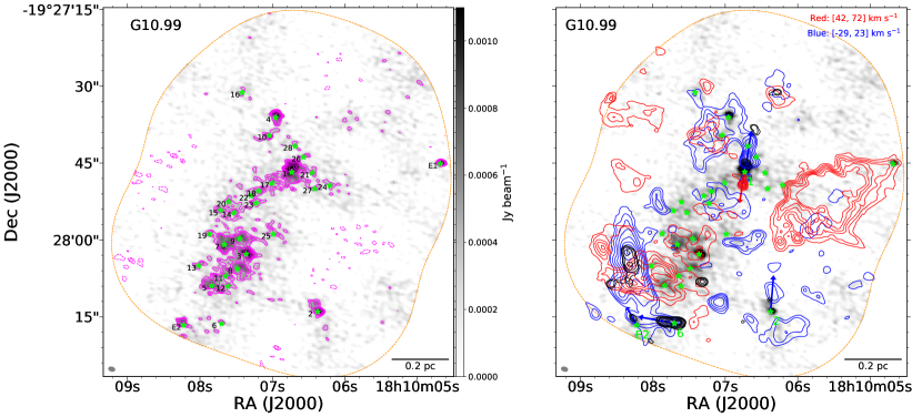
Figure 1: ALMA 1.3 mm continuum, CO and SiO velocity integrated intensities images for G10.99. The gray images in both panels show the 1.3 mm continuum emission. Dashed orange contour shows 20% of the sensitivity level of the mosaic in the ALMA continuum image. The green stars indicate the identified dense cores. Left: ALMA 1.3 mm continuum image. The contour levels are (-4, -3, 3, 4, 5, 7, 10, 14, 20)$\times\sigma$, with $\sigma=$0.115 mJy beam^-1. Right: The blue-shifted (blue contours) and red-shifted (red contours) components of CO emission, and SiO velocity-integrated intensity (black contours, integration range is between 7 and 39 km s^-1) overlaid on the continuum emission. The blue and red contours levels are (4, 6, 9, 13, 18, 24, 31)$\times\sigma$, where the $\sigma$ are 0.05 Jy beam^-1 km s^-1 and 0.03 Jy beam^-1 km s^-1 for blue and red contours, respectively. The black contours are (3, 4, 5, 6, 7, 8, 9)$\times\sigma$, with $\sigma=$ 0.02 Jy beam^-1 km s^-1. On the left side panel, black numbers correspond to the name of all cores. On the right side panel, the green numbers indicate only the cores associated with molecular outflows. The beam size of continuum image is shown on the bottom left of each panel. The complete figure set (7 images, see Figure 10) is available in the online journal.

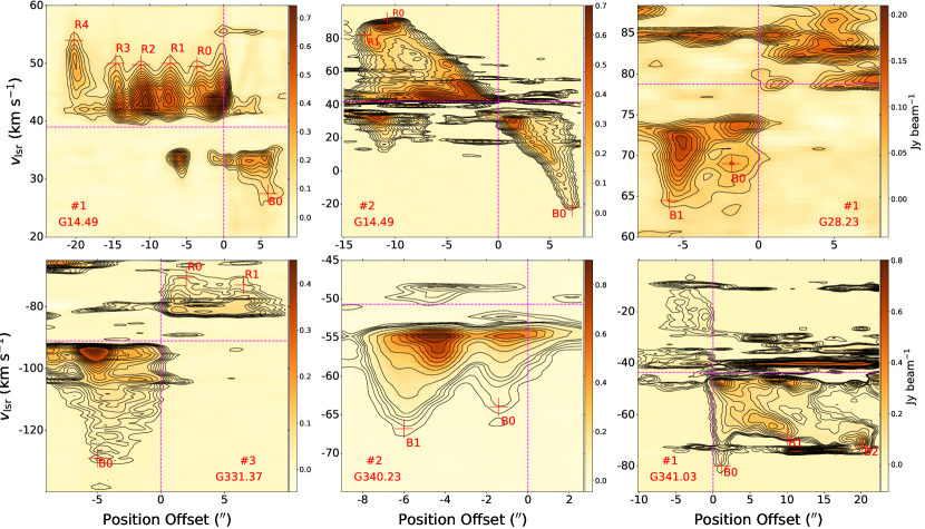
Figure 2: Position-velocity (PV) diagram of the CO emission. The cut of the PV diagrams is along the CO outflows that are indicated by the arrows in Figure 1. The name of the associated core and clump is displayed in each panel. The red crosses mark the locations of the detected knots. The vertical and horizontal dashed fuchsia lines represent the position and velocity of dense core, respectively. The contour levels are (-3, 3 to 30 by 2 steps)$\times\sigma$, with $\sigma=$40 mJy beam^-1, for #1–G14.49. The contour levels are (-5, 5, 7, 10, 14, 19, 25, 32, 40 to 100 by 10 steps)$\times\sigma$, with $\sigma=$5 mJy beam^-1, for #2–G14.49. The contour levels are (-5, 5 to 23 by 2 steps)$\times\sigma$, with $\sigma=$6 mJy beam^-1, for #1–G28.23. The contour levels are (-5, 5 to 21 by 2 steps, and 25 to 80 by 5 steps)$\times\sigma$, with $\sigma=$4 mJy beam^-1, for #3–G331.37. The contour levels are ( -5, 5 to 20 by 3 steps, and 30 to 180 by 20 steps)$\times\sigma$, with $\sigma=$4.5 mJy beam^-1, for #2–G340.23. The contour levels are (-5, 5 to 20 by 3 steps, and 30 to 150 by 10 steps)$\times\sigma$, with $\sigma=$3 mJy beam^-1, for #1–G341.03. The cut of the #1–G341.03 PV diagram is along the northwest-southeast CO outflow.

2 Observations

Observations of the 12 infrared dark clouds (IRDCs) were performed with ALMA in Band 6 (224 GHz; 1.34 mm) using the main 12 m array, the Atacama Compact 7 m Array (ACA; Morita Array), and the total power (TP; Project ID: 2015.1.01539.S; PI: Sanhueza).

Some sources were observed in different configurations (see Table 2 in Sanhueza et al., 2019). The uv-taper was used in those sources to obtain a similar synthesized beam size of  1$\farcs$2 for each source (see also Sanhueza et al., 2019). The primary beam sizes are 25$\farcs$2 and 44$\farcs$6 for the 12 m array and ACA at the center frequency of 224 GHz, respectively. We made two Nyquist-sampled mosaics with the 12 m array (10-pointings) and ACA (3-pointings), covering about 0.97 arcmin² within the 20% power point, except for the IRDC G028.273$-$00.167 that was observed with 11 and 5-pointings. These mosaics were designed to cover a significant portion of the clumps, as defined by single-dish continuum images. All sources were observed with the same correlator setup.

Data calibration was performed using the CASA software package versions 4.5.3, 4.6, and 4.7, while imaging was carried out using CASA 5.4 (McMullin et al., 2007). Continuum images were obtained by averaging line-free channels over the observed spectral windows with a Briggs’s robust weighting of 0.5 of the visibilities. This achieved an average 1$\sigma$ root mean square (rms) noise level of $\sim$0.1 mJy beam^-1. The beam size for each clump is summarized in Table 1. For detected molecular lines (N₂D⁺ 3-2, DCN 3-2, DCO⁺ 3-2, CCD 3-2, ¹³CS 5-4, SiO 5-4, C¹⁸O 2-1, CO 2-1, and H₂CO 3-2, CH₃OH 4-3), we used a Briggs’s robust weighting of 2.0 (natural weighting) for imaging. Using the feathering technique, the 12m and 7m array molecular line data was combined with the TP data in order to recover the missing flux. This yields a 1$\sigma$ rms noise level of $\sim$0.06 K per channel of 0.17 km s^-1 for the first six lines and $\sim$0.02 K per channel of 1.3 km s^-1 for the last four lines.

3 Results and Analysis

Using the CO 2-1 and SiO 5-4 lines, we searched for molecular outflows toward the 301 embedded dense cores that have been revealed in the 1.3 mm continuum images of the 12 IRDC clumps. Sanhueza et al. (2019) focused on 294 cores, excluding 7 cores located at the edge of the images (20%-30% power point). We have included these 7 cores in our analysis because some of them are associated with molecular outflows. CO was used as the primary outflow tracer, while SiO was used as a secondary outflow tracer. Figure 1 shows an overview of the identified molecular outflows toward one clump. All images shown in the paper use the 12 m array data only and prior to primary beam correction, while all measured fluxes are derived from the combined data (including 12 m, 7 m, and TP) and corrected for the primary beam attenuation.

3.1 Outflow Detection

For the identification of outflows, we use the 12 m array data only. We follow the procedure described below to identify CO outflows: (1) Using DS9, we inspect the position-position-velocity (PPV) data cubes of the CO emission to determine the velocity ranges of the blue- and red-shifted components with respect to the cloud emission. (2) These velocity ranges are used to generate the velocity integrated intensity maps (moment-0) for both blue- and red-shifted components, which in conjunction with the channel maps and the CO line profiles are used to determine the direction of CO outflows. (3) The position-velocity (PV) diagram, which is cut along the identified CO outflow, combined with the channel maps and line profiles are further used to carefully refine the velocity range of each CO outflow to exclude the ambient gas from the cloud. However, in some cases (e.g., the outflows associated with core #3/#5/#6/#17/#32 in the G341.03 clump) the outflows cannot be well separated from nearby overlapping outflows or ambient gas and those outflows were marked as “Marginal”. For the outflows, that are unambiguously associated with a dense core, and are unambiguously distinguishable from nearby outflows and the ambient gas, were marked as “Definitive”. Among the 43 identified outflows, 33 are defined as definitive outflows, while the remaining are classified as marginal (Table 2). The derived physical parameters of the definitive outflows are more reliable than those of the marginal outflows (Section 3.2).

The velocity range ($\bigtriangleup v$) of outflows are defined where the emission avoid environment gas around the system velocity and higher than the 2$\sigma$ noise level, where $\sigma$ is the rms noise level in the line-free channels. The outflow lobes are defined where the corresponding velocity integrated intensity is higher than the 4$\sigma$ noise level, where $\sigma$ is the rms of the integrated intensity map. After defining outflows following the procedure, we use the 12 m, 7 m, and TP combined data to compute outflow parameters. Using the CO line, we have identified 43 molecular outflows toward 41 out of 301 dense cores (Table 2), with a detection rate of 14% (41/301). There are 2 cores associated with 2 molecular outflows. Among these 41 cores, 28 are associated with SiO emission (detection rate of 9%). The relatively low detection rate of SiO is likely due to the fact that the excitation energy and critical density of the SiO 5-4 transition are much higher than that of the CO 2-1 transition (e.g., Li et al., 2019a). There are three clumps (G332.96, G340.17 and G340.22) without molecular outflows detected in the CO or SiO line.

Sixteen outflows show bipolar morphology. In addition, we find a bipolar outflow without any association with dense cores in G331.37 (Figure 1), which could be due to the associated core mass below our detection limit (e.g., Pillai et al., 2019). The remaining 27 outflows present a unipolar morphology. The fraction of outflows showing unipolar morphology is 63%, higher than the fraction of 25% and 40% in W43-MM1 and in a sample of protocluster (Baug et al., 2020; Nony et al., 2020), respectively. Based on the CO emission, we find that the ambient gas is frequently found around the dense core. Therefore, we might fail to identify some low-velocity and/or weak outflows because their emission can be confused with the ambient gas. We cannot completely rule out the possibility that this bias contributes to the high fraction of unipolar outflows.

There are 2 cores, #2 of G327.11 (#2–G327.11) and #1 of G341.03 (#1–G341.03), showing two bipolar morphology outflows in CO emission (see Figure 1). The two bipolar outflows are approximately perpendicular to each other in both #2–G327.11 and #1–G341.03, which suggests that these cores encompass multiple protostars with accretion disks that are perpendicular to each other. Alternatively, these two cores may be showing outflows with wide opening angles. However, we favour the first scenario because wide angles are expected in much more evolved sources and those expected in these IRDCs that properties are consistent with early stages of evolution (Arce et al., 2007).

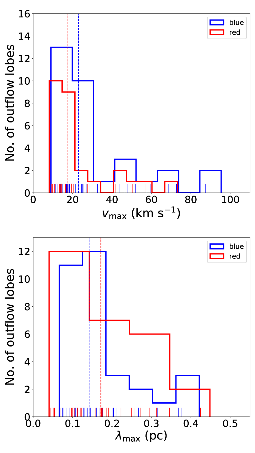
Figure 3: Upper and bottom panels show the distributions of the maximum velocity ($v_{\rm max}$) and maximum projected distance ($\lambda_{\rm max}$) of the CO outflow, respectively. Red histogram represents the red-shifted gas, while blue histogram represents the blue-shifted gas. The blue and red dashed lines indicate the median value of blue-shifted and red-shifted, respectively.

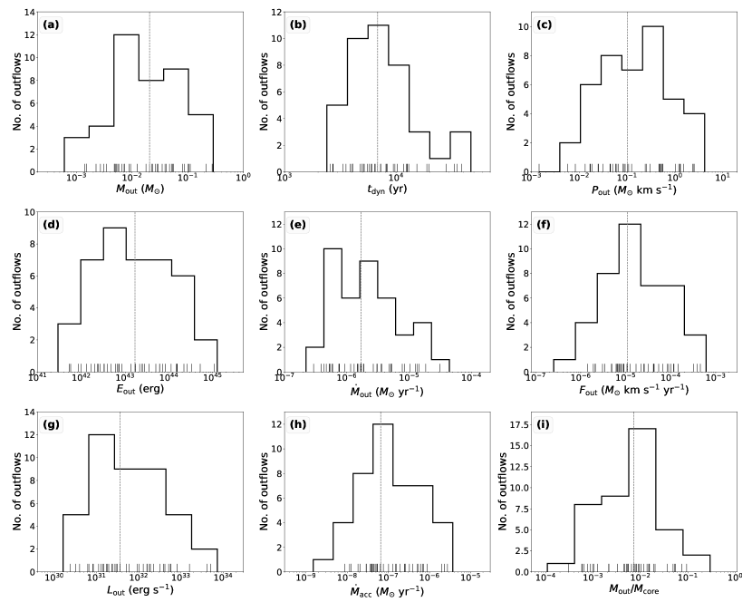
Figure 4: Panel (a) to (i) shows the distributions of total outflow mass ($M_{\rm out}$), outflow dynamical timescale ($t_{\rm dyn}$), outflow momentum ($P_{\rm out}$), outflow energy ($E_{\rm out}$), outflow rate ($\dot{M}_{\rm out}$), mechanical force($F_{\rm out}$), outflow luminosity ($L_{\rm out}$), accretion rate ($\dot{M}_{\rm acc}$), and ratio ($M_{\rm out}/M_{\rm core}$) of outflow mass to core mass, respectively. The black dashed lines indicate the median value of each parameter.

The velocity integrated intensity is integrated over the entire velocity range of the identified red/blue line wings. There are several exceptions because some foreground and/or background CO emission is found in the velocity range of line wings (see Figure 2). Figure 1 shows the CO velocity integrated intensity map for each clump. The directions of molecular outflows are indicated by arrows. There are 3 weak CO outflows (#4–G327.11, #1–G341.03 and #2–G341.03), identified through PV-diagrams and channel maps. The emission from these weak outflows is much smaller than the velocity ranges used in the figures (Figure 1), resulting in a dilution of the signal making the weak outflows not visible in the figures.

The core systemic velocity is determined by the centroid velocity, $v_{\rm lsr}$, of the N₂D⁺ 3-2 line, while the DCO⁺ 3-2 line is used when the N₂D⁺ line is undetected. The C¹⁸O 2-1 line is used when both the N₂D⁺ and DCO⁺ lines are undetected. The maximum detected velocities (e.g., $v_{\rm max(r)}={\rm max}(v_{\rm r})$, where $v_{\rm r}=|v_{\rm CO}-v_{\rm lsr}|$ is a variable representing the red-shifted outflow velocity with respect to the core systemic velocity) of the CO red- and blue-shifted lobes with respect to the core systemic velocity range from 9 to up to 95 km s^-1. Figure 3 shows the distributions of $v_{\rm max}$ for the detected outflow lobes. The mean and median of $v_{\rm max}$ are 28 and 21 km s^-1, respectively. There are 9 cores associated with a CO outflow with line wings at velocities greater than 30 km s^-1 ($v_{\rm max}>30$) with respect to the core systemic velocity. The maximum lengths of the CO outflow red-/blue-shifted lobes projected on the plane of the sky ($\lambda_{\rm max}$) are in the range of 0.04 and 0.45 pc (Figure 3), with the mean and median values of 0.25 and 0.23 pc, respectively. Note that both $v_{\rm max}$ and $\lambda_{\rm max}$ estimated here should be considered as lower limits because the outflow emission is limited by the sensitivity of the observations, can be confused by nearby outflows and/or line-of-sight emission that is not associated with the natal cloud, and these parameters have not been corrected for the outflow inclination.

3.2 Outflow Parameters

Since the SiO abundances vary significantly from region to region and its emission is much weaker than the CO, we used the CO data to compute the outflow parameters by assuming that the CO line wing emission is optically thin. Following the approach delineated in Li et al. (2019a) (see Appendix A), we estimated the main physical parameters of each outflow, including the mass ($M_{\rm out}$), momentum ($P_{\rm out}$), energy ($E_{\rm out}$), dynamical timescale ($t_{\rm dyn}$), outflow rate ($\dot{M}_{\rm out}$), outflow energy rate (also known as outflow luminosity, $L_{\rm out}$) and mechanical force ($F_{\rm out}$). The calculation of these outflow parameters is summarized in Appendix A.

The outflow masses range from 0.001 to 0.32 $M_{\odot}$, with a mean mass of 0.044 $M_{\odot}$ (Figure 4 and Table 2). We compare the outflow mass to the core mass, and find that the outflow mass is smaller than 10% of the core mass (Figure 4), except for #13-G341.03 outflows, with a mass of 22% of the core mass. This is owing to the outflow of #13-G341.03 is significantly contaminated by the nearby outflow driven by the #3–G341.03 (see Figure 1). The estimated outflow dynamical timescales range from 0.1 $\times\,10^{4}$ to 3.2 $\times\,10^{4}$ yr. We used the outflow mass and dynamical time to estimate the outflow ejection rates, which are between 2.4 $\times\,10^{-7}$ and 5.0 $\times\,10^{-5}$ $M_{\odot}$ yr^-1. The outflow momenta range from 0.2 $\times\,10^{-2}$ to 3.4 $M_{\odot}$ km s^-1. The outflow energies are between 0.4 $\times\,10^{42}$ and 1.2 $\times\,10^{45}$ erg. The outflow luminosity can be estimated by dividing the outflow energy by the outflow dynamical timescale, $L_{\rm out}=E_{\rm out}/t_{\rm dyn}$, which are in the range of 0.2 $\times\,10^{31}$ and 2.1 $\times\,10^{34}$ erg s^-1. The outflow mechanical force is computed using the outflow momentum and dynamical timescale, $F_{\rm out}=P_{\rm out}/t_{\rm dyn}$, which is between 0.3 $\times\,10^{-6}$ and 9.8 $\times\,10^{-4}$ $M_{\odot}$ km s^-1 yr^-1.

Assuming that: (1) the outflows are driven by protostellar winds from accretion disks (e.g., Keto, 2003; McKee & Tan, 2003); (2) the wind and molecular gas interface is efficiently mixed (Richer et al., 2000); (3) the momentum is conserved between the wind and the outflow, with no loss of momentum to the surrounding cloud, one can estimate the accretion rate, $\dot{M}_{\rm acc}=k\,\dot{M}_{\rm w}$, using the mass-loss rate ($\dot{M}_{\rm w}$) of the wind that is inferred from the associated outflow mechanical force, $\dot{M}_{\rm w}v_{\rm w}=F_{\rm out}$. We assume a ratio of $k\,=\,\dot{M}_{\rm acc}/\dot{M}_{\rm w}\,=\,3$ between the mass accretion rate and the mass ejection rate (Tomisaka, 1998; Shu et al., 2000). The wind velocity $v_{\rm w}$ is adopted to be 500 km s^-1, which ranges from a few km s^-1 to over 1000 km s^-1 in young stellar objects (YSOs; Bally, 2016). The derived accretion rate ranges from 2.0 $\times\,10^{-9}$ to 3.8 $\times\,10^{-6}$ $M_{\odot}$ yr^-1, with a mean value of 4.9 $\times\,10^{-7}$ $M_{\odot}$ yr^-1. These values are much smaller than the predicted accretion rate (order $10^{-4}-10^{-3}$ $M_{\odot}$ yr^-1) in some high-mass star formation models (e.g., McKee & Tan, 2003; Wang et al., 2010). See discussions of accretion rate below in Section 4.2.1.

Since the inclination angle of the outflow axes is not known, the outflow parameters and accretion rate have not been corrected for their inclination for all of outflows. The estimated outflow parameters of each outflow are summarized in Table 2 and Figure 4.

3.3 Outflow-driven turbulence

Stars generate vigorous outflows during their formation process. These outflows transfer not only mass but also energy into their parent molecular cloud. Therefore, outflow feedback is considered one of the mechanisms to replenish the internal turbulence (Li & Nakamura, 2006; Graves et al., 2010; Arce et al., 2010; Nakamura et al., 2011a; Krumholz et al., 2014; Nakamura & Li, 2014; Li et al., 2015; Offner & Chaban, 2017). To assess whether the outflow-induced turbulence can play a significant role in replenishing the internal turbulence for the extremely early phase of high-mass star formation, we estimate the ratio of the outflow energy rate ($L_{\rm out}$) to turbulent energy dissipation rate ($\dot{E}_{\rm turb}$), $r_{L}=L_{\rm out}/\dot{E}_{\rm turb}$.

The turbulent energy ($E_{\rm turb}$) is given by

$$E_{\rm turb}=\frac{1}{2}M(\sqrt{3}\;\sigma_{\rm los,1D})^{2},$$ (1)

where $\sigma_{\rm los,1D}$ is the one-dimensional velocity dispersion along the line of sight, which is

$$\sigma_{\rm los,1D}=\frac{\sqrt{\triangle v_{\rm FWHM}^{2}-\triangle v_{\rm chan}^{2}}}{2\sqrt{2\rm\;ln\;2}},$$ (2)

Here, the $\triangle v_{\rm chan}$ and $\triangle v_{\rm FWHM}$ are the channel width and the full width at the half maximum (FWHM) of the line emission, respectively. Using the physical properties of the clumps (Table 1), we obtained the turbulent energies ranging from 5.4 $\times$ 10⁴⁵ to 4.4 $\times$ 10⁴⁷ erg (Table 3).

The turbulent dissipation rate ($\dot{E}_{\rm turb}$) can be calculated as (McKee & Ostriker, 2007)

$$\dot{E}_{\rm turb}=\frac{E_{\rm turb}}{t_{\rm diss}},$$ (3)

where dissipation time, $t_{\rm diss}$, has two different definitions based on numerical simulations. In the first approach, the turbulent dissipation time of the cloud is given by (e.g., McKee & Ostriker, 2007)

$$t_{\rm diss}\sim 0.5\frac{R_{\rm cl}}{\sigma_{\rm 1D}},$$ (4)

where $R_{\rm cl}$ is the cloud radius. The obtained turbulent dissipation times are between 5.8 $\times$ 10⁴ and 3.6 $\times$ 10⁵ yr, yielding turbulent dissipation rates of $(0.5-114.7)\times\,10^{33}$ erg s^-1 (Table 3). The obtained $t_{\rm diss}$ is comparable to the estimated value of a few 10⁵ yr in the Perseus region (Arce et al., 2010), while is smaller than the reported value of 1.6 $\times$ 10⁷ yr in the Taurus molecular cloud (Li et al., 2015). The $r_{L}$ lies in the range of 0.004–4.05, with a median value of 0.08 (Table 3). The range of values is much lower than those found in relatively evolved star forming-regions, for instance, 0.8$-$12.4 in Perseus, 2$-$7 in $\rho$ Ophiuchi, 0.6$-$3 in Serpens South (Arce et al., 2010; Nakamura et al., 2011b; Plunkett et al., 2015a).

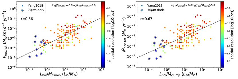
Figure 5: Left: plot of the $L_{\rm bol}/M_{\rm clump}$ against the $F_{\rm out,tot}$. The correlation coefficient is 0.66 between $L_{\rm bol}/M_{\rm clump}$ and $F_{\rm out,tot}$ in the Spearman-rank correlation test. The solid black line is the least-squares fitting result ${\rm log}(F_{\rm out,tot})=0.8{\rm log}(L_{\rm bol}/M_{\rm clump})-3.6$ (see also Yang et al., 2018). The colorbar indicates the spatial resolution. Right: plot of the $L_{\rm bol}/M_{\rm clump}$ versus the $\dot{M}_{\rm acc,tot}$. There is a strong correlation between $L_{\rm bol}/M_{\rm clump}$ and $\dot{M}_{\rm acc,tot}$ with a correlation coefficient of 0.67. The solid black line is the best least-squares fitting result ${\rm log}(\dot{M}_{\rm acc,tot})=0.8{\rm log}(L_{\rm bol}/M_{\rm clump})-5.8$. The colorbar indicates the spatial resolution.

In the second approach, the turbulent dissipation time can be defined as (e.g., Mac Low, 1999)

$$t_{\rm diss}\sim 3.9\frac{\kappa}{M_{\rm rms}}t_{\rm ff},$$ (5)

where $M_{\rm rms}=v_{\rm los,3D}/c_{\rm s}=\sqrt{3}v_{\rm los,1D}/c_{\rm s}$ is the Mach number of the turbulence, $t_{\rm ff}=\sqrt{3\pi/32G\rho}$ is the free-fall timescale, $\kappa=\lambda_{d}/\lambda_{J}$ is the ratio of the driving wavelength ($\lambda_{d}$) to the Jeans wavelength ($\lambda_{J}=c_{\rm s}(\pi/G\rho)^{1/2}$). The average volume density of a clump is calculated by $\rho$ = $3M_{\rm cl}/4\pi R_{\rm cl}^{3}$. For a continuous outflow, the outflow lobe length can be used to approximate the turbulence driving wavelength according to numerical simulations (Nakamura & Li, 2007; Cunningham et al., 2009). The estimated $t_{\rm diss}$ ranges from 1.3 $\times$ 10⁴ to 1.5 $\times$ 10⁵ yr, resulting in turbulent dissipation rates of $(3.8-109.5)\times\,10^{33}$ erg s^-1 (Table 3). Using the derived $\dot{E}_{\rm turb}$, we find that the $r_{L}$ is between 0.001 and 0.54, with a median value of 0.02.

4 Discussion

4.1 Biases on Outflow Parameters

CO is the most frequently used tracer for studying molecular outflows driven by protostars. Note that the outflow parameters estimated from the CO line emission are only a lower limit considering the observational biases: (1) CO fails to trace the outflow in low-density regions, which can be traced by other low-density gas tracers (e.g., Hi 21 cm and Cii 157 $\mu\rm m$ lines); (2) optical depth effects on the outflow parameters; (3) the limited sensitivity of our observations. On average, the combined effects of the above mentioned biases could lead to a factor of $\sim$10 underestimate in the outflow mass and dynamical properties (Dunham et al., 2014). On the other hand, the unknown inclinations of the outflow axis with respect to the line of sight can also introduce an uncertainty on the outflow parameters estimations (Dunham et al., 2014; Li et al., 2019a). Assuming all orientations have equal probability from parallel ($\theta=0^{\circ}$) to perpendicular ($\theta=90^{\circ}$) to the line of sight, one can compute an mean inclination angle $\langle\theta\rangle\approx 57^{\circ}.3$. For the mean inclination angle, the correction factors are 1.9 for $v_{\rm out}$; 1.2 for $\lambda_{\rm out}$; 0.6 for $t_{\rm dyn}$; 1.9 for $P_{\rm out}$; 3.4 for $E_{\rm out}$; and 1.7 for $\dot{M}_{\rm out}$ (see, Dunham et al., 2014; Li et al., 2019a).

4.2 Outflow Properties

To study the relationship between the outflow properties and their associated dense cores, we have compared core masses and outflow parameters, including the outflow dynamical timescale, outflow maximum velocity, outflow projected distance, outflow mass, outflow momentum, outflow energy, outflow rate, outflow luminosity, and mechanical force. There are no clear correlations between core masses and outflow parameters, with the exception of outflow dynamical timescale, which appears to show a positive correlation with the core mass. In Section 4.2.1, we discuss the accretion rate and outflow mechanical force. Then, we discuss the relationship between the outflow dynamical timescale and the core mass in Section 4.2.2. The discussion of emission knots in the molecular outflows is presented in Section 4.2.3.

4.2.1 Accretion Rate and Outflow Mechanical Force

Using the CO outflows, the estimated protostellar accretion rates are between 2.0 $\times\,10^{-9}$ to 3.8 $\times\,10^{-6}$ $M_{\odot}$ yr^-1, with a mean value of 4.9 $\times\,10^{-7}$ $M_{\odot}$ yr^-1. These values are comparable to those derived toward other 70 $\mu\rm m$ and 24 $\mu\rm m$ dark massive cores (Lu et al., 2015; Zhang et al., 2015; Li et al., 2019a) and some low/intermediate-mass cores (van Kempen et al., 2016; Feddersen et al., 2020b) following the same approach, while they are much smaller than the typical value of a few $\times$($10^{-5}-10^{-4}$) $M_{\odot}$ yr^-1 reported in much more evolved massive cores (e.g., 24 $\mu\rm m$ bright cores, 4.5 $\mu\rm m$ bright cores and UCHII regions, Qiu & Zhang, 2009; Qiu et al., 2009; López-Sepulcre et al., 2010; Duarte-Cabral et al., 2013; Liu et al., 2017; Lu et al., 2018). This indicates that the accretion rates likely increase with the evolution of star formation.

The bolometric luminosity-to-mass ratio ($L/M$) is believed to be a indicator of the evolutionary phase of star formation. The early evolutionary phase correspond to a low $L/M$ value, while later stages correspond to higher values of $L/M$ (Molinari et al., 2008). Figure 5 shows the luminosity-to-mass ratio ($L_{\rm bol}/M_{\rm clump}$) versus the total outflow mechanical forces ($F_{\rm out,tot}$), for our 70 $\mu\rm m$ dark clumps, together with high-mass clumps from Yang et al. (2018). In the latter clumps, the observations have an angular resolution of 15^′′ (Yang et al., 2018), which should not be able to spatially resolve the outflows for the embedded cores. Thus, we added the outflow parameters (i.e., mechanical force $F_{\rm out,tot}$ = $\sum F_{\rm out}$ and accretion rate $\dot{M}_{\rm acc,tot}$ = $\sum\dot{M}_{\rm acc}$) for each core within a clump for our 70 $\mu\rm m$ dark sources. The bolometric luminosities of our clumps are estimated with the procedure introduced by Contreras et al. (2017) (see their Equation 3). The $L_{\rm bol}/M_{\rm clump}$ and $F_{\rm out,tot}$ shows a strong positive correlation, over nearly $\sim$4 order of magnitude in $L_{\rm bol}/M_{\rm clump}$ and $\sim$5 order of magnitude in $F_{\rm out,tot}$ (see also, Yang et al., 2018). The correlation coefficient is 0.66 with a p-value of $2\,\times\,10^{-22}$ in a Spearman-rank correlation test, which assess monotonic relationships. This indicates that outflow forces increase with protostellar evolution in the high-mass regime. The outflow forces in our clumps are relatively lower compared to other high-mass clumps in Yang et al. (2018), which is likely due to a later evolutionary stage as evidenced by the high $L_{\rm bol}/M_{\rm clump}$ value.

As mentioned in Section 3.2, we can estimate the accretion rate using the outflow force. Here, we adopt a wind velocity of 500 km s^-1 and a $\dot{M}_{\rm acc}/\dot{M}_{\rm w}$ of 3 for all the clumps in Yang et al. (2018). Figure 5 shows a strong positive correlation between the total accretion rate ($\dot{M}_{\rm acc,tot}$) and $L_{\rm bol}/M_{\rm clump}$. The Spearman-rank correlation test returns a correlation coefficient of 0.67 with a p-value of $3\,\times\,10^{-2}$. This strong correlation suggests that the accretion rates indeed increase with the evolution of star formation.

For the dense cores detected CO outflows, the estimated accretion rates (a few $10^{-7}\,M_{\odot}$ yr^-1) are $\sim$3 orders of magnitude lower than the predicted values of high-mass star formation models (McKee & Tan, 2003; Wang et al., 2010; Kuiper et al., 2016). The computed accretion rates might be increased by a factor of $\sim$2 orders of magnitude in the most extreme cases that have the highest ratios of accretion to ejection rates, which varies from 1.4 to even 100 in different observational and theoretical studies (e.g., Sheikhnezami et al., 2012; Ellerbroek et al., 2013; Frank et al., 2014; Kuiper et al., 2016). Assuming a constant ratio of the accretion to mass ejection rate, we found that the estimated accretion rates of these protostars are indeed significantly lower than the predicted values in the theoretical studies, even after accounting for the effects of opacity and inclination angle.

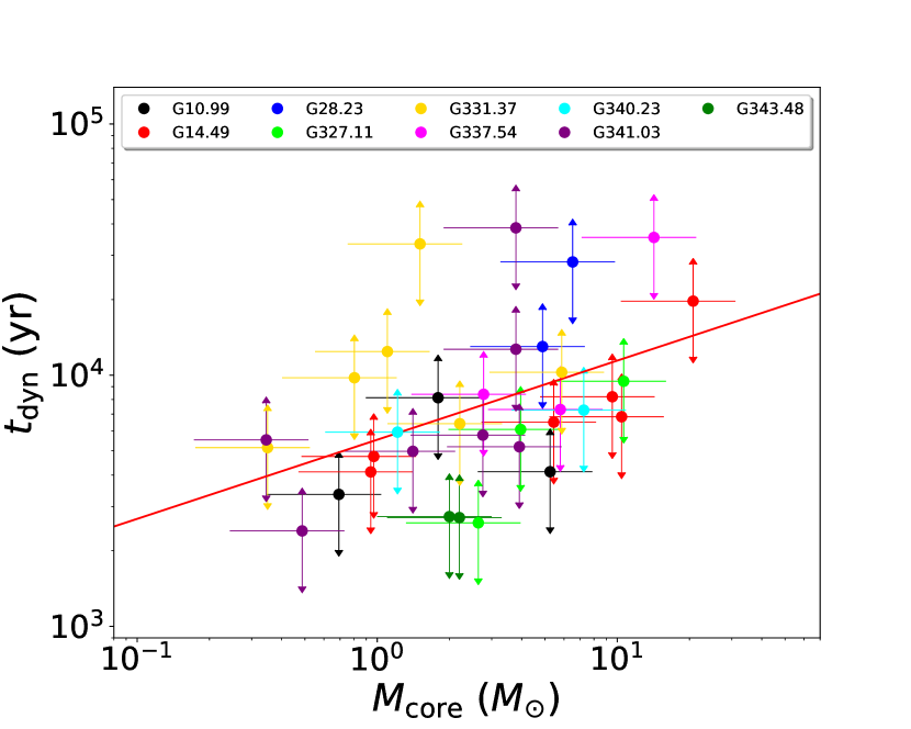
Figure 6: Core mass versus the outflow dynamical timescale for all cores associated to CO outflows. The Spearman-rank correlation test returns a correlation with a coefficient of 0.51. The solid red line is the best least-squares fitting result with ${\rm log}(t_{\rm dyn})=0.32{\rm log}(M_{\rm core})+3.74$. The error bars of $M_{\rm core}$ correspond to its uncertainty of 50% (Sanhueza et al., 2017, 2019). The error bars of $t_{\rm dyn}$ correspond to the mean inclination angle ($\langle\theta\rangle\approx 57^{\circ}.3$) correction.

4.2.2 Outflow Dynamical Timescale

Figure 6 shows the relation between the outflow dynamical timescale ($t_{\rm dyn}$) and the core mass ($M_{\rm core}$). We have removed marginal outflows in this plot to eliminate the effect of the ambiguous outflows. Consistent with what Li et al. (2019a) found for a sample of 70 $\mu\rm m$ dark clumps, the outflow dynamical timescale increases with the core mass. The correlation coefficient is 0.51 with a p-value of 2$\times$10^-3 in a Spearman-rank correlation test. This indicates a moderate correlation between the outflow dynamical timescale and the core mass. The $t_{\rm dyn}-M_{\rm core}$ relation suggests that more massive cores tend to have a longer outflow dynamical timescale than less massive cores. Since outflows are a natural consequence of accretion, the positive relation between $t_{\rm dyn}$ and $M_{\rm core}$ suggests that the more massive cores have a longer accretion history than less massive ones in a protocluster. Note that the measurement of outflow dynamical timescales is affected by observational effects such as the unknown inclination angle of the outflow axes. The positive correlation between $t_{\rm dyn}$ and $M_{\rm core}$ persists unless the inclination angles of the outflows are close to 0^∘ or 90 ^∘ (see Figure 6).

4.2.3 Episodic Ejection

From Figure 1, we find that 6 out of 43 molecular outflows show a series of knots in the integrated intensity map. Figure 2 presents their PV diagrams along the axis of outflows. The Hubble Law and Hubble Wedge features are clearly seen in the PV diagram of some outflows (Lada & Fich, 1996; Arce & Goodman, 2001). Episodic variation of, e.g., mass-loss rate and flow velocity, in a protostellar ejection can produce internal shocks. This mechanism has been proposed to produce emission knots (which correspond to the Hubble Wedge in the PV diagram) in molecular outflows (Arce & Goodman, 2001; Arce et al., 2007; Vorobyov et al., 2018; Cheng et al., 2019; Rohde et al., 2019). Since the accretion is episodic, the outflow as a natural consequence of the accretion is episodic as well (Kuiper et al., 2015; Bally, 2016; Cesaroni et al., 2018). The Hubble Wedge features are found to be independent of the core mass, associated with both low-mass and high-mass cores (see Figures 1 and 2). This suggests that episodic accretion-driven outflows begin in the earliest phase of protostellar evolution for low-mass, intermediate-mass, and high-mass protostellar cores in a protocluster.

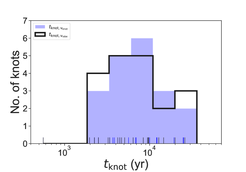
Figure 7: The distribution of knots dynamical timescales estimated by $v_{\rm knot}$ and $v_{\rm lobe}$.

In Section 3.2 (Appendix A), we used the maximum velocity and the projected distance of the CO outflows to estimate the outflow dynamical timescale, $t_{\rm dyn}=\lambda_{\rm out}/v_{\rm max}$. Similarly, we can estimate the dynamical timescale of the identified knots using their projected distance ($\lambda_{\rm knot}$) and corresponding velocity ($v_{\rm knot}$) with respect to the associated core, $t_{\rm knot}=\lambda_{\rm knot}/v_{\rm knot}$. From Figure  2, one notes that the knots have different velocities. Therefore, we use $v_{\rm knot}$, instead of the mean velocity of detected knots ($v_{\rm lobe}=\langle v_{\rm knot}\rangle$) as used in Nony et al. (2020), when calculating the knot dynamical timescale.

We visually follow contours in the PV-diagram to define the velocity and the projected distance of detected knots (see Figure  2). The locations of knots in each outflow are presented in Figure  2. The mean $v_{\rm knot}$ for all knots is 22 km s^-1, ranging from 10 to 60 km s^-1. The $\lambda_{\rm knot}$ are between 0.02 and 0.39 pc, with a mean value of 0.15 pc. Uncertainties are conservatively estimated as 2 km s^-1 for velocities (3 times of channel width), and 0$\farcs$5 for lengths (about half of angular resolution). The estimated dynamical timescales of knot range from 6 $\times\,10^{2}$ to 2.5 $\times\,10^{4}$ yr, with the mean and median value of 8.6 $\times\,10^{3}$ and 6.6 $\times\,10^{3}$ yr, respectively (see Table 4). These values are higher than the value of $100-6000$ yr found for low-mass YSOs (e.g., Santiago-García et al., 2009; Plunkett et al., 2015b), but comparable to the value of $400-10^{4}$ yr for high-mass YSOs (e.g., W43-MM1; Nony et al., 2020) and the predicted timescale of a few$\times$($10^{3}-10^{4}$) yr in the model of Vorobyov et al. (2018).

To study the time span between consecutive ejection events, we compute the timescale difference between knots, $\triangle t_{\rm knot}$ = $t_{{\rm knot},i+1}$ - $t_{{\rm knot},i}$, which ranges from 3.6 $\times\,10^{2}$ to 7.2 $\times\,10^{3}$ yr, with a mean value of 4.4 $\times\,10^{3}$ yr. The derived $\triangle t_{\rm knot}$ is much larger than the reported value of $\sim$500 yr for W43-MM1 (Nony et al., 2020), even accounting for the typical projection correction and the typical measured uncertainty.

By comparing the knots timescales estimated by $v_{\rm knot}$ and $v_{\rm lobe}$, we find that the two results agree very well with each other (see Figure 7). This suggests that the different knot timescales between these studies are not due to the use of two different methods. The different $\triangle t_{\rm knot}$ could be due to the different period of episodic ejection between two samples, considering that they are significantly different in the evolutionary stages. Our 70 $\mu\rm m$ dark cores are in a much earlier stage than those infrared bright cores in W43-MM1 (Nony et al., 2020). If this scenario is correct, the discrepancy likely implies that the ejection episodicity timescale is not constant over time and accretion bursts may be more often at later stages of evolution.

The consecutive Hubble Wedge features seen in the PV diagram are not necessarily successive in time for the evolved objects in a very clustered environment. This is because they have had enough time to experience numerous repeated ejection events. Therefore, they can create a series in time with nonconsecutive Hubble Wedge features. In this IRDC study, the detected outflows are still in an extremely early phase of protostellar evolution, thus the outflows likely trace the early accretion activities. This could be another possibility to cause the different $\triangle t_{\rm knot}$ between different evolutionary stages of star formation. The observations of W43-MM1 by Nony et al. (2020) have a spatial resolution of $\sim$2400 AU, which is higher than our observations ($\sim$4000–7500 AU). Given the different spatial resolutions between the two studies, we cannot fully rule out the possibility that the different $\triangle t_{\rm knot}$ is due to the effect of spatial resolutions as higher spatial resolutions help to resolve more individual knots. All these possibilities can be tested with the high spatial resolution observations of a larger sample of dense cores encompassing different evolutionary stages of star formation.

4.3 Outflow Impact on the Clumps

The mechanical energy in outflows is found to be comparable to the turbulent energy in the more evolved sources of both low- and high-mass star formation (eg., Beuther et al., 2002; Zhang et al., 2005; Arce et al., 2010; Nakamura & Li, 2014). In addition, the outflow-induced turbulence can sustain the internal turbulence (Arce et al., 2010; Nakamura & Li, 2014; Li et al., 2015). In contrast, we find that the total outflow energy (2.7 $\times\,10^{42}\,-\,2.1\,\times\,10^{45}$ erg) in the sample is significantly lower than the turbulent energy (3.1 $\times\,10^{45}\,-\,4.2\,\times\,10^{47}$ erg). This indicates that outflows do not have the energy for driving the turbulence in these clumps at the current epoch. In addition, the total outflow ejected mass occupies only a tiny fraction of the clump mass, with a ratio of 6 $\times$ 10^-6 – 3 $\times$ 10^-4 (see Table 3).

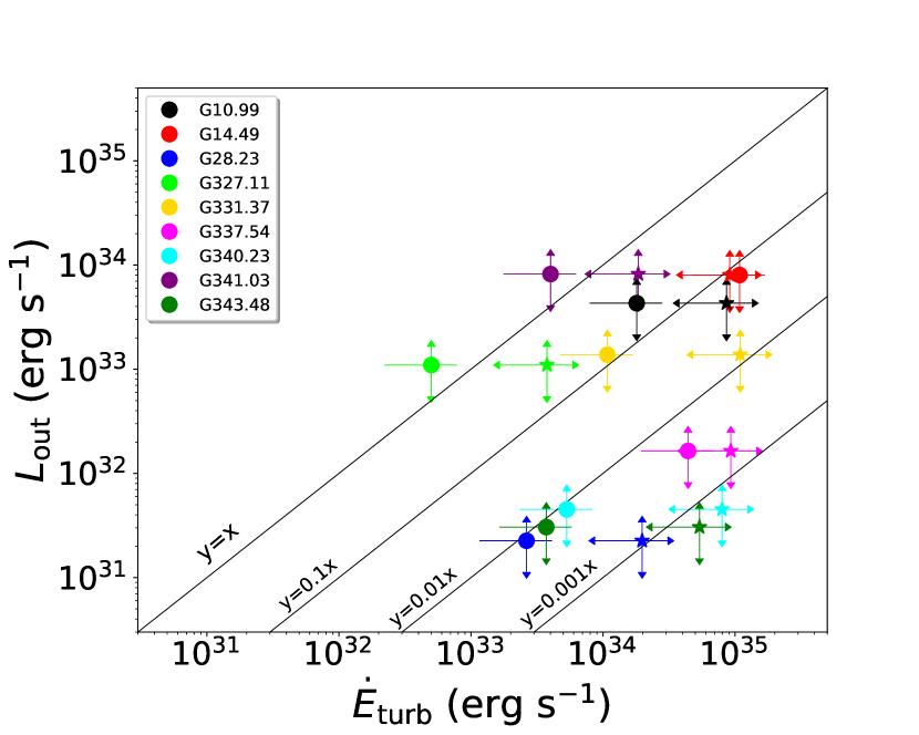
Figure 8: The turbulent dissipation rate versus the outflow luminosity. The filled circles and filled stars represent the turbulent dissipation rate computed by the first (Equation 4) and second (Equation 5) approaches, respectively.

Figure 8 shows the outflow luminosity versus the turbulent dissipation rate. As mentioned in Section 3.3, we compute the turbulent dissipation time ($t_{\rm diss}$) using two different approaches. The determined $t_{\rm diss}$ using the first approach (Equation 4) is larger than that of the second approach (Equation 5). The latter is depending on the length of outflows, which may introduce uncertainties in the estimation of $t_{\rm diss}$. Overall, the results from both approaches are consistent (Figure 8 and Table 3), the outflow luminosity is much smaller than the turbulent dissipation rate in the majority of clumps, except for G327.11 and G341.03, which have relatively larger $r_{\rm L}$. The computed $r_{\rm L}$ is smaller as compared to the values found in other works for more evolved sources (e.g., Arce et al., 2010; Nakamura et al., 2011b; Plunkett et al., 2015a). This indicates that the outflow-induced turbulence produced by these early stage cores is not yet severely affecting the internal clump turbulence.

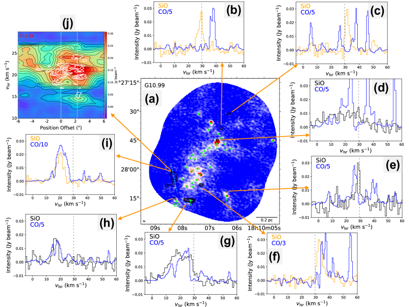
Figure 9: Panel a: SiO velocity-integrated intensity (black contours, integration range is between 7 and 39 km s^-1) overlaid on the continuum emission of G10.09. The contours are (-4, -3, 3, 4, 5, 6, 7, 8, 9)$\times\sigma$, with $\sigma=$ 0.02 Jy beam^-1 km s^-1. Green stars indicate the dense cores revealed by dust continuum. The continuum beam size is plotted at the bottom-left corner. The cyan dashed lines indicate the PV cuts path (panel j and k). Panel b-i: spectra of SiO 5-4 (orange and black) and CO 3-2 (blue) toward several positions across the G10.99. Panel b, c, f and i show the SiO (orange) and CO profiles toward the regions where SiO emission appear to neither associated with outflows nor dense cores. The black vertical dashed line is the clump velocity. Panel j: PV diagram of the CO (color-scale and black contours) and SiO (white contours) emission across the SiO contours (cyan dashed lines). The white contours are (3, 4, 5, 6)$\times\sigma$, with $\sigma$ = 0.008 Jy beam^-1. The black contours are (7, 14, 21, 28 …)$\times\sigma$, with $\sigma$ = 0.004 Jy beam^-1. The white dashed lines indicate the peak positions of SiO contours.

From Table 3, we note that the G327.11 has the narrowest line width and the lowest mass, resulting in the lowest turbulent energy and the lowest turbulent dissipation rate among the sample. This seems to be the reason why G327.11 can have the outflow-induced turbulence required for replenishing the clump turbulence. G341.03 is another exception with sufficient outflow-induced turbulence to maintain the clump turbulence. Using the CO line emission, we find that it has the highest outflow detection rate (27%) and has the largest outflow luminosity among the whole IRDC sample. This implies that outflows can become a major source of turbulence in the clumps when the majority of the embedded cores evolve to launch strong molecular outflows.

Strong outflows generated by young stars have a disruptive impact on their natal clouds. Similarly, the outflow energy ($E_{\rm out}$) can be compared to the gravitational binding energy of clouds, $E_{\rm grav}=GM_{\rm cl}^{2}/R_{\rm cl}$, for evaluating the potential disruptive effects of outflows on their clouds. The gravitational energy of clouds ranges from 7.4 $\times\,10^{46}$ to 5.3 $\times\,10^{48}$ erg, which is much larger than the total outflow energy for each clump. The ratio of $E_{\rm out}/E_{\rm grav}$ is between 2 $\times\,10^{-5}$ and 8 $\times\,10^{-3}$, which indicates that the disruptive impact of these outflows on their parent clouds is, for now, negligible for all the clump sample. This is because these clumps are still in extremely early evolutionary stages of star formation and have not yet been severely affected by protostellar feedback (consistent with being 24 and 70 $\mu$m dark). Therefore, these clumps are ideal objects for studying the initial conditions of high-mass star and cluster formation.

4.4 SiO Emission Unrelated to CO Outflows

SiO has been widely used to trace shocked gas, such as those associated with protostellar outflows and jets (Zhang et al., 1999, 2000; Hirano et al., 2006; Palau et al., 2006; Codella et al., 2013; Leurini et al., 2014; Li et al., 2019b, a). This is because the SiO formation is closely linked to the shock activities, which releases Si atoms from dust grains into gas phase through sputtering or vaporization (Schilke et al., 1997).

A total of 28 out of 43 CO outflows are detected in the SiO 5-4 line (see Figure 1). The outflows seen in the SiO emission are more compact as compared with the CO spatial distribution, and appears to follow the outflow direction defined by CO. In addition, the SiO emission is significantly weaker than the CO emission. This difference is most likely due to the higher excitation conditions (density, energy) and different chemical conditions required by the SiO 5-4 transition with respect to the CO 2-1 transition (e.g., Li et al., 2019b). The comparison of outflow velocities measured by the CO line shows no difference between the outflows with SiO detection and without SiO detection. This indicates that the production of SiO requires other conditions (e.g., density and temperature) in addition to the appropriate velocity.

From Figure 1, it is interesting to note that there is strong SiO emission that is neither associated with CO outflows nor dense cores. As previously mentioned, SiO emission is closely related to the shock phenomena, therefore its presence suggests that there are strong shocks unrelated to star formation activities such as outflows or jets. Figure 9 shows an overview of the SiO spectra toward G10.99. The SiO and CO emission, which is associated with protostellar outflows, appear to be comparable in the line central velocity (e.g., panel d, e, g and h of Figure 9). However, we note that there is also SiO emission that appears to be unrelated to outflows and dense cores.

Assuming optically thin and local thermodynamic equilibrium (LTE) condition for the SiO emission, the SiO column densities estimated to be $N$(SiO) = $8.1\,\times\,10^{11}-5.9\,\times\,10^{13}\,\rm cm^{-2}$, with a median value of $4.7\,\times\,10^{12}\,\rm cm^{-2}$. The derived SiO column densities are comparable to that measured in high- and low-mass star forming regions (e.g., Bachiller et al., 1991; Hirano et al., 2006; Fernández-López et al., 2013). To derive SiO abundances, we estimate the H₂ column densities from CO line (see Appendix A). The SiO abundance is found to be $X$(SiO) = $1.1\,\times\,10^{-9}-1.6\,\times\,10^{-7}$ with a median value of $1.0\,\times\,10^{-8}$. Overall, we find no significant differences in the SiO column densities for the SiO gas components associated with and without CO outflows, except for G10.19, which shows relatively higher SiO column densities toward the CO outflows as compared to the regions without CO outflow counterparts.

In most cases the shocked regions traced by SiO emission without CO outflow counterpart are associated with multiple velocity components, as revealed by the CO emission (PV diagram and channel maps). In some cases, the velocities of the SiO emission are around the clump velocity (see panel b and c of Figure 9), while some of them are offset from the clump velocity (see panel i of Figure 9). The interaction between different velocity components can enhances the local shock activities, resulting an enhancement in the SiO emission (Jiménez-Serra et al., 2010). Figure 9 shows the PV diagram of the CO emission across the SiO contours for one sub-regions, the bright SiO emission appears to be at the location of a velocity shear (panel j in Figure 9); interfaces between different velocity components. The FWHM line widths of SiO measured toward these shocked regions are $\geqslant$ 5 km s^-1, which are broader than the narrow line width of $\sim$0.8 km s^-1 measured for the widespread SiO emission along the IRDC G035.39$-$0.33 (Jiménez-Serra et al., 2010). The broad SiO emission is a further hint of gas movement due to the interaction between different gas components. This indicates that the shocks that produce this SiO emission most likely arise from colliding or intersecting gas flows. For the other clumps, we also find that some of the SiO emission is located at the positions where velocity shears in the CO emission may be present. This SiO emission is most likely a result of collision or intersection of gas flows as well.

On the other hand, we find that some of the SiO emission regions show no signs of velocity shears in the CO emission (e.g., the regions corresponding to the spectra of panel b and c). In addition to collision/intersection of gas flows, the large/small-scale converging flows, the larger scale collapse, a population of undetected low-mass objects and some dense cores outside of the map could also create shocks, resulting in an enhancement in the SiO emission (e.g., Jiménez-Serra et al., 2010; Csengeri et al., 2011; Sanhueza et al., 2013; Duarte-Cabral et al., 2014). Unfortunately, we can not distinguish between these possibilities with the data at hand. They can be tested by spatially resolving both large and small scale gas motions with reliable dense gas tracers (e.g, N₂H⁺) or searching for deeply embedded distributed low-mass protostars in near-infrared observations as has been done in another IRDC by Foster et al. (2014).

5 Conclusions

In this paper, we analyzed the data from ASHES obtained with ALMA to study molecular outflow and shock properties in 12 massive 70 $\mu\rm m$ dark clumps.

1. Outflow activities revealed by either CO or SiO emission are found in 9 out of the 12 clumps observed. We successfully identified 43 molecular outflows in 41 out of 301 dense cores, with an outflow detection rate of 14% in the CO 2-1 emission. Among the 41 cores, 12 cores are associated with single bipolar outflows, 2 cores host two bipolar outflows, while the remaining 27 cores have single uniploar outflows. The CO outflows are detected in both low-mass and high-mass cores. The maximum velocity of CO outflows reaches up to 95 km s^-1 with respect to the systemic velocity. These results suggest that most of 70 $\mu\rm m$ dark clumps already host protostars, and thus they cannot be assumed to be prestellar without deep interferometric observations.

2. The estimated protostellar accretion rates range from 2.0 $\times\,10^{-9}$ to 3.8 $\times\,10^{-6}$ $M_{\odot}$ yr^-1 for the dense cores detected outflows, which is smaller than the typical value reported in more evolved cores. The comparison of the total accretion rates and $L_{\rm bol}/M_{\rm clump}$ in different evolutionary stages indicates that the accretion rates increase with the evolution of star formation. For this sample, the median ratio of outflow mass to core mass is about $8\,\times\,10^{-3}$, while the median ratio of total outflow mass to clump mass is about $2\,\times\,10^{-4}$.

3. We found a positive correlation between the outflow dynamical timescale and the gas mass of dense cores. The observed increase of outflow dynamical timescales towards the more massive cores indicates that the accretion history is longer in the more massive cores compared to the less massive cores.

4. We identified six episodic molecular outflows associated to cores of all masses. This indicates that episodic outflows begin in the earliest stages of protostellar evolution for different masses of cores. The computed dynamical timescales ($t_{\rm knot}$) of episodic outflow events are in the range $6\times 10^{2}$ to $2.5\times 10^{4}$ yr with time span ($\triangle t_{\rm knot}$) between consecutive episodic outflow events of $3.6\times 10^{2}-7.2\times 10^{3}$ yr. The $\triangle t_{\rm knot}$ is much longer than the value ($\sim$500 yr) found in more evolved cores in W43-MM1 (Nony et al., 2020), which indicates that the ejection episodicity timescale is likely not constant over time and accretion bursts may be more frequently at later stages of evolution in a cluster environment.

5. In ASHES, the mechanical energy of outflows is much smaller than values from more evolved high-mass star-forming regions, for which outflow mechanical energy is comparable to the kinetic energy arising from the internal gas motions. The total outflow luminosity is smaller than the turbulent dissipation rate in the majority of the clumps. This suggests that the outflow feedback can not replenish the internal turbulence in the majority of the sources at the current epoch. In addition, the disruptive impact of the outflows on their parent clouds is negligible for this sample.

6. We found strong SiO emission not associated with protostellar outflows. This finding suggests that protostellar outflows are not the sole mechanism responsible for SiO production and emission. Alternatively, other processes, such as large scale collisions or intersection of converging flows, can give rise to shocks.

Appendix A Estimate of outflow parameters

Assuming that local thermodynamic equilibrium (LTE), we can estimate the CO column density ($N_{\rm CO}$), outflow mass ($M_{\rm out}$), momentum ($P_{\rm out}$), energy ($E_{\rm out}$), based on the CO emission (Bally & Lada, 1983; Cabrit & Bertout, 1992; Mangum & Shirley, 2015):

$$N_{\rm CO}(\rm cm^{-2})=1.08\times 10^{13}(T_{\rm ex}+0.92)\;{\rm exp}\left(\frac{16.59}{T_{\rm ex}}\right)\int\frac{\tau_{21}}{1-e^{\tau_{21}}}T_{\rm B}dv,$$ (A1)

$$M_{\rm out}={d^{2}}\left[\frac{\rm H_{2}}{\rm CO}\right]\overline{m}_{\rm H_{2}}\int_{\Omega}N_{\rm CO}(\Omega)d\Omega,$$ (A2)

$$P_{\rm out}=M_{\rm r}v_{r}+M_{b}v_{\rm b},$$ (A3)

$$E_{\rm out}=\frac{1}{2}M_{\rm r}v_{\rm r}^{2}+\frac{1}{2}M_{\rm b}v_{\rm b}^{2},$$ (A4)

Using the CO outflow projected distance ($\lambda_{\rm max}$), we compute the outflow dynamical timescale ($t_{\rm dyn}$), outflow rate ($\dot{M}_{\rm out}$), outflow luminosity ($L_{\rm out}$), and mechanical force ($F_{\rm out}$):

$$t_{\rm dyn}=\frac{\lambda_{\rm max}}{(v_{\rm max(b)}+v_{\rm max(r)})/2},$$ (A5)

$$\dot{M}_{\rm out}=\frac{M_{\rm out}}{t_{\rm dyn}},$$ (A6)

$$L_{\rm out}=\frac{E_{\rm out}}{t_{\rm dyn}},$$ (A7)

$$F_{\rm out}=\frac{P_{\rm out}}{t_{\rm dyn}}.$$ (A8)

Here, $dv$ is the velocity interval in km s^-1, $T_{\rm ex}$ is the line excitation temperature, $\tau_{21}$ is the optical depth, $T_{\rm B}$ is brightness temperature in K, $\Omega$ is the total solid angle that the flow subtends, $d$ is the source distance, $v_{\rm max(b)}$ and $v_{\rm max(r)}$ are the maximum velocities of CO blue-shifted and red-shifted emission, respectively. $M_{\rm r}$ and $M_{\rm b}$ are the gas masse of CO outflows at the corresponding blue-shifted ($v_{\rm b}$) and red-shifted ($v_{\rm r}$) velocities, respectively.

A range of excitation temperatures, from 10 to 60 K, has been used to calculate the column density in order to understand the effect of excitation temperatures on the CO column density. The estimated CO column density agree within a factor of 1.5 in this temperature range, which indicates that the CO column density dose not significantly depend on the temperature. In this work, we assume that CO emission is optically thin in the line wing and that the dust temperature approximate the excitation temperature of outflow gas (see Table 1), and adopt the CO-to-H₂ abundance of 10^-4, $\left[\frac{\rm H_{\rm 2}}{\rm C\rm O}\right]$ = 10⁴ (Blake et al., 1987), and mean molecular mass per hydrogen molecule $\overline{m}_{\rm H_{2}}$ = 2.72m_H. The CO velocity integrated intensity has been corrected for primary beam attenuation, while the inclination of the outflow axis with respect to the line of sight have not been corrected in the estimation of the outflow parameters.

Table 1: Physical Properties of the Clumps and Observational Parameters.

Name	abbreviation	R.A.	Decl.	Dist.	$M_{\rm cl}$	$R_{\rm cl}$	$L_{\rm bol}$	$v_{\rm lsr}$	$\sigma$	$T_{dust}$	$\sum_{\rm cl}$	$n_{\rm cl}$	$\theta_{\rm cont}$	$\theta_{\rm CO}$	$\theta_{\rm SiO}$
		(J2000)	(J2000)	(kpc)	($M_{\odot}$)	(pc [′′])	(L⊙)	(km s-1)	(km s-1)	(K)	(g cm-2)	($10^{4}$ cm-3)	(′′$\times$ ′′)	(′′$\times$ ′′)	(′′$\times$ ′′)
G010.991$-$00.082	G10.99	18:10:06.65	$-$19.27.50.7	3.7	2230	0.49 (27)	467	29.5	1.27	12.0	0.50	5.3	1.29 $\times$ 0.86	1.44 $\times$ 0.99	1.57 $\times$ 1.08
G014.492$-$00.139	G14.49	18:17:22.03	$-$16.25.01.9	3.9	5200	0.44 (23)	1211	41.1	1.68	13.0	1.10	13.0	1.29 $\times$ 0.85	1.43 $\times$ 0.99	1.51 $\times$ 1.05
G028.273$-$00.167	G28.23	18:43:31.00	$-$04.13.18.1	5.1	1520	0.59 (24)	402	80.0	0.81	12.0	0.28	2.4	1.28 $\times$ 1.20	1.44 $\times$ 1.36	1.50 $\times$ 1.43
G327.116$-$00.294	G327.11	15:50:57.18	$-$54.30.33.6	3.9	580	0.39 (20)	408	$-$58.9	0.56	14.3	0.26	3.5	1.32 $\times$ 1.11	1.51 $\times$ 1.26	1.60 $\times$ 1.34
G331.372$-$00.116	G331.27	16:11:34.10	$-$51.35.00.1	5.4	1640	0.63 (24)	776	$-$87.8	1.29	14.0	0.20	1.7	1.34 $\times$ 1.09	1.54 $\times$ 1.24	1.63 $\times$ 1.32
G332.969$-$00.029	G332.96	16:18:31.61	$-$50.25.03.1	4.4	730	0.59 (28)	195	$-$66.6	1.41	12.6	0.10	0.9	1.35 $\times$ 1.08	1.55 $\times$ 1.22	1.64 $\times$ 1.30
G337.541$-$00.082	G337.54	16:37:58.48	$-$47.09.05.1	4.0	1180	0.42 (22)	293	$-$54.6	2.01	12.0	0.40	5.0	1.29 $\times$ 1.18	1.45 $\times$ 1.34	1.56 $\times$ 1.45
G340.179$-$00.242	G240.17	16:48:40.88	$-$45.16.01.1	4.1	1470	0.74 (37)	645	$-$53.7	1.48	14.0	0.12	0.9	1.41 $\times$ 1.29	1.51 $\times$ 1.48	1.56 $\times$ 1.53
G340.222$-$00.167	G340.22	16:48:30.83	$-$45.11.05.8	4.0	760	0.36 (19)	728	$-$51.3	3.04	15.0	0.38	5.5	1.40 $\times$ 1.28	1.49 $\times$ 1.47	1.53 $\times$ 1.51
G340.232$-$00.146	G340.23	16:48:27.56	$-$45.09.51.9	3.9	710	0.48 (25)	332	$-$50.8	1.23	14.0	0.15	1.7	1.39 $\times$ 1.26	1.49 $\times$ 1.47	1.53 $\times$ 1.50
G341.039$-$00.114	G341.03	16:51:14.11	$-$44.31.27.2	3.6	1070	0.47 (27)	634	$-$43.0	0.97	14.3	0.26	2.9	1.30 $\times$ 1.18	1.47 $\times$ 1.34	1.70 $\times$ 1.54
G343.489$-$00.416	G343.48	17:01:01.19	$-$42.48.11.0	2.9	810	0.42 (29)	85	$-$29.0	1.00	10.3	0.30	3.8	1.30 $\times$ 1.18	1.47 $\times$ 1.34	1.70 $\times$ 1.53

Table 2: Parameters of Identified CO Outflows.

Source	Core ID		$v_{\rm lsr}$	$\Delta v$	$M_{\rm out}$	$P_{\rm out}$	$E_{\rm out}$	$\lambda_{\rm out}$	$t_{\rm dyn}$	$\dot{M}_{\rm out}$	$F_{\rm out}$	$L_{\rm out}$	Confidence
			(km s-1)	(km s-1)	(10-2 M⊙)	(M⊙ km s-1)	(1043 erg)	(pc)	(104 yr)	(10-6 M⊙ yr-1)	(10-4 M⊙ km s-1 yr-1)	(1032 erg s-1)
G10.99	1	blue	29.5	[-29.9, 15.5]	1.59	0.348	8.84	0.112	0.18	8.61	1.88	15.16	M
		red	29.5	[42.6, 102.8]	2.57	0.965	43.50	0.159	0.21	12.13	4.55	65.06	M
	2	blue	30.1	[17.2, 28.0]	1.25	0.066	0.44	0.104	0.81	1.54	0.08	0.17	M
	6	blue	26.9	[1.9, 17.2]	1.54	0.231	3.61	0.085	0.34	4.59	0.69	3.41	D
	E2	blue	27.3	[9.6, 16.5]	1.11	0.160	2.35	0.075	0.41	2.69	0.39	1.80	D
G14.49	1	blue	38.6	[9.8, 34.5]	2.52	0.296	4.02	0.145	0.49	5.13	0.60	2.60	D
		red	38.6	[42.1, 66.3]	32.22	2.523	27.11	0.425	1.50	21.43	1.68	5.72	D
	2	blue	41.8	[-27.0, 33.2]	5.31	1.025	26.10	0.161	0.23	23.18	4.48	36.16	D
		red	41.8	[47.8, 92.3]	16.95	3.371	88.26	0.256	0.50	34.18	6.80	56.43	D
	3	blue	41.2	[8.5, 33.9]	9.52	1.127	14.11	0.169	0.51	18.77	2.22	8.83	D
		red	41.2	[42.8, 62.5]	2.16	0.138	1.48	0.097	0.45	4.84	0.31	1.05	D
	4	blue	40.3	[-7.4, 34.5]	10.95	1.585	32.15	0.127	0.26	41.95	6.07	39.06	D
		red	40.3	[42.1, 97.5]	29.72	1.820	10.05	0.346	0.59	50.29	3.08	5.39	D
	14	red	40.2	[42.8, 51.0]	0.75	0.033	0.18	0.052	0.47	1.58	0.07	0.12	D
	29	blue	39.1	[20.6, 34.5]	5.28	0.486	5.13	0.078	0.41	12.81	1.18	3.95	D
G28.23	1	blue	78.8	[61.3, 74.6]	3.05	0.227	1.95	0.204	1.14	2.68	0.20	0.54	D
		red	78.8	[81.0, 88.6]	4.02	0.160	0.74	0.191	1.90	2.12	0.08	0.12	D
	6	red	80.0	[83.5, 89.2]	0.74	0.036	0.19	0.122	1.30	0.57	0.03	0.05	D
G327.11	1	blue	-59.1	[-79.4, -62.8]	4.69	0.393	3.48	0.138	0.67	7.01	0.59	1.65	D
		red	-59.1	[-52.0, -41.9]	0.22	0.030	0.41	0.053	0.30	0.74	0.10	0.43	D
	2	blue1	-59.3	[-146.7, -62.8]	1.53	0.030	2.14	0.091	0.10	14.96	0.30	6.65	M
		red1	-59.3	[-50.8, -43.2]	2.05	0.233	2.74	0.175	1.06	1.92	0.22	0.82	M
		blue2	-59.3	[-132.1, -62.8]	1.74	0.213	10.83	0.154	0.21	8.36	1.03	16.54	M
		red2	-59.3	[-50.8, -12.7]	3.82	0.791	18.77	0.223	0.47	8.17	1.69	12.74	M
	3	red	-59.6	[-52.1, -43.2]	0.18	0.022	0.28	0.043	0.26	0.71	0.09	0.35	D
	4	red	-59.6	[-58.4, -51.4]	0.95	0.034	0.15	0.037	0.45	2.12	0.08	0.10	D
G331.37	3	blue	-88.0	[-140.0, -92.4]	14.77	1.910	35.89	0.210	0.40	37.35	4.83	28.77	D
		red	-88.0	[-82.9, -67.6]	9.44	0.876	9.35	0.250	1.20	7.88	0.73	2.47	D
	4	blue	-88.0	[-103.2, -94.3]	5.44	0.567	6.22	0.159	1.03	5.30	0.55	1.92	D
	5	red	-88.0	[-77.8, -70.8]	0.56	0.068	0.85	0.113	0.64	0.87	0.11	0.42	D
	14	blue	-87.5	[-102.5, -93.0]	6.09	0.609	6.51	0.268	1.74	3.49	0.35	1.18	D
		red	-87.5	[-77.8, -70.8]	0.80	0.096	1.18	0.273	1.60	0.50	0.06	0.23	D
	19	blue	-88.0	[-108.2, -98.1]	2.62	0.465	8.30	0.129	0.51	5.10	0.90	5.11	D
	29	red	-88.0	[-77.8, -70.8]	0.56	0.071	0.91	0.172	0.98	0.58	0.07	0.30	D
G337.54	1	blue	-54.5	[-76.3, -55.9]	11.65	0.673	5.74	0.200	0.92	12.64	0.73	1.97	D
		red	-54.5	[-52.1, -40.7]	18.22	0.972	6.38	0.449	3.07	5.94	0.32	0.66	D
	2	blue	-54.8	[-69.3, -56.6]	5.71	0.304	2.07	0.377	2.59	2.21	0.12	0.25	M
		red	-54.8	[-50.9, -40.7]	3.04	0.196	1.45	0.313	2.14	1.42	0.09	0.21	M
	3	red	-54.5	[-53.0, -40.7]	1.52	0.071	0.48	0.099	0.73	2.08	0.10	0.21	D
	9	red	-55.6	[-53.4, -40.1]	3.08	0.126	0.84	0.120	0.84	3.67	0.15	0.32	D
G340.23	1	blue	-50.5	[-68.8, -52.9]	0.93	0.046	0.28	0.111	0.59	1.57	0.08	0.15	D
	2	blue	-50.7	[-70.1, -58.0]	1.44	0.132	1.30	0.144	0.73	1.99	0.18	0.57	D
G341.03	1	blue1	-46.1	[-67.5, -46.6]	4.89	0.184	1.15	0.315	1.44	3.39	0.13	0.25	D
		red1	-46.1	[-42.1, -37.0]	0.76	0.035	0.17	0.296	3.18	0.24	0.01	0.02	D
		blue2	-46.1	[-89.7, -46.6]	3.80	0.517	9.02	0.368	1.36	2.79	0.38	2.10	D
		red2	-46.1	[-42.1, -4.2]	4.09	0.939	26.94	0.187	0.44	9.40	2.16	19.63	D
	2	blue	-43.0	[-54.2, -44.0]	0.36	0.002	0.04	0.066	0.58	0.63	0.00	0.02	D
	3	blue	-43.3	[-70.1, -49.1]	3.66	0.663	12.54	0.421	1.54	2.38	0.43	2.58	M
	4	blue	-43.7	[-69.4, -45.3]	1.11	0.058	0.56	0.136	0.52	2.14	0.11	0.34	D
	5	blue	-43.3	[-52.3, -46.6]	0.35	0.017	0.09	0.108	1.17	0.30	0.01	0.02	M
	6	blue	-42.2	[-56.1, -47.8]	2.96	0.253	2.27	0.267	1.89	1.57	0.13	0.38	M
	13	blue	-43.6	[-138.6, -46.6]	2.87	1.764	117.08	0.176	0.18	15.90	9.76	205.41	D
		red	-43.6	[-39.0, -15.5]	0.92	0.059	0.39	0.173	2.09	0.44	0.03	0.06	D
	14	blue	-42.3	[-70.7, -56.1]	0.83	0.159	3.16	0.144	0.50	1.67	0.32	2.01	D
	17	blue	-42.9	[-70.1, -49.1]	0.75	0.105	1.73	0.067	0.24	3.14	0.44	2.29	D
	32	blue	-43.0	[-59.9, -45.9]	0.27	0.016	0.12	0.067	0.39	0.70	0.04	0.10	M
G343.48	1	red	-28.7	[-19.8, -9.6]	0.09	0.009	0.09	0.050	0.25	0.37	0.04	0.12	M
	2	red	-28.7	[-21.0, -9.6]	0.16	0.009	0.06	0.040	0.27	0.59	0.03	0.07	D
	3	red	-28.4	[-24.9, -13.4]	0.22	0.015	0.11	0.054	0.27	0.80	0.05	0.13	D
Mean					4.41	0.480	9.70	0.172	0.87	7.32	1.05	9.58
Median					2.16	0.196	2.14	0.145	0.58	2.69	0.30	0.82
Minimum					0.09	0.002	0.04	0.037	0.10	0.24	0.003	0.02
Maximum					32.22	3.371	117.08	0.449	3.18	50.29	9.76	205.41

Table 3: Assessment of Outflow Impact on Clumps.

Name	$E_{\rm out}$	$L_{\rm out}$	$E_{\rm grav}$	$E_{\rm turb}$	$t_{\rm diss}$	$\dot{E}_{\rm turb}$	$r_{L}$		$t_{\rm diss}$	$\dot{E}_{\rm turb}$	$r_{L}$	$E_{\rm out}/E_{\rm grav}$	$E_{\rm out}/E_{\rm turb}$	$M_{\rm out}/M_{\rm clump}$
	(1044 erg)	(1033 erg s-1)	(1046 erg)	(1046 erg)	(105 yr)	(1033 erg s-1)			(105 yr)	(1033 erg s-1)
(1)	(2)	(3)	(4)	(5)	(6)	(7)	(8)		(9)	(10)	(11)	(12)	(13)	(14)
G10.99	5.87	4.69	86.82	10.72	1.89	18.00	0.261		0.39	86.21	0.054	6.76E-04	5.48E-03	3.62E-05
G14.49	20.86	8.88	525.74	43.76	1.28	108.26	0.082		1.52	91.22	0.097	3.97E-04	4.77E-03	2.22E-04
G28.23	0.29	0.03	33.50	2.97	3.57	2.64	0.013		0.48	19.79	0.002	8.59E-05	9.70E-04	5.14E-05
G327.11	3.88	2.03	7.38	0.54	3.42	0.50	4.053		0.45	3.76	0.539	5.26E-03	7.19E-02	2.62E-04
G331.37	6.92	2.00	36.52	8.13	2.39	10.79	0.186		0.24	109.49	0.018	1.90E-03	8.51E-03	2.46E-04
G332.96	…	…	7.73	4.33	2.05	6.70	…		…	…	…	…	…	…
G337.54	1.57	0.16	28.36	14.22	1.02	44.09	0.004		0.49	92.91	0.002	5.54E-04	1.11E-03	2.92E-04
G340.17	…	…	24.98	9.60	2.45	12.44	…		…	…	…	…	…	…
G340.22	…	…	13.73	20.95	0.58	114.66	…		…	…	…	…	…	…
G340.23	0.16	0.07	8.98	3.20	1.91	5.31	0.013		0.13	79.74	0.001	1.76E-04	4.93E-04	3.35E-05
G341.03	17.53	8.43	20.84	3.00	2.37	4.01	2.103		0.51	18.50	0.455	8.41E-03	5.85E-02	2.58E-04
G343.48	0.03	0.03	13.36	2.41	2.06	3.72	0.008		0.14	53.83	0.001	1.99E-05	1.10E-04	5.84E-06

Table 4: Parameters of CO Knots.

Clump	Core ID	Knot	$\lambda_{\rm knot}$	$v_{\rm knot}$	$t_{\rm knot}$	$\triangle v_{\rm knot}$
			(pc)	(km s-1)	(103 yr)	(103 yr)
G14.49	1	B0	0.11	11.50	9.75	…
		R0	0.07	10.50	6.41	…
		R1	0.14	11.00	12.23	5.83
		R2	0.21	10.80	19.38	7.15
		R3	0.28	11.00	24.81	5.42
		R4	0.39	15.00	25.17	0.36
	2	B0	0.14	60.00	2.24	…
		R0	0.21	52.50	3.84	…
		R1	0.25	43.00	5.65	1.81
G28.23	1	B0	0.04	9.76	4.46	…
		B1	0.15	14.26	10.01	5.55
G331.37	3	B0	0.13	37.93	3.39	…
		R0	0.05	20.57	2.50	…
		R1	0.07	18.07	3.70	1.20
G340.23	2	B0	0.03	13.31	1.97	…
		B1	0.11	16.11	6.96	5.00
G341.03	1	B0	0.02	36.45	0.56	…
		B1	0.17	24.95	6.83	6.26
		B2	0.35	28.45	12.09	5.27
Mean			0.15	23.43	8.52	4.38
Median			0.14	16.11	6.41	5.35
Minimum			0.02	9.76	0.56	0.36
Maximum			0.39	60.00	25.17	7.15

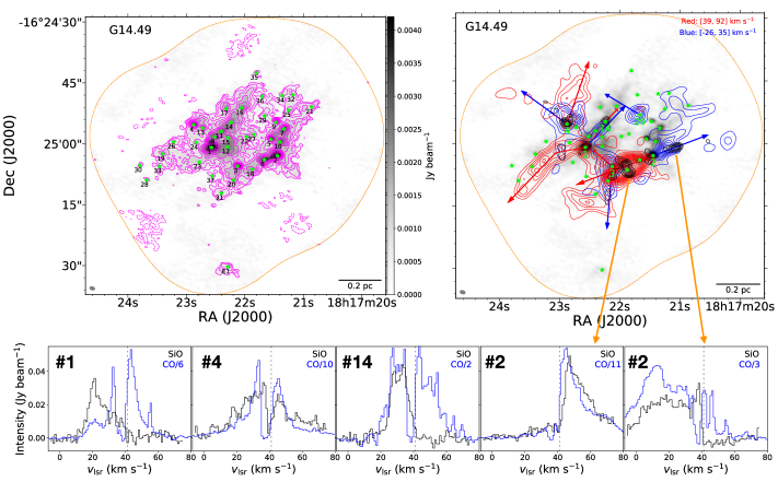
(a)

Figure 10: Presented here are individual plots for Figure 1 which are available as the online material. Dashed orange contour shows 20% of the sensitivity level of the mosaic in the ALMA continuum image. The green stars indicate the identified dense cores. Upper left: ALMA 1.3 mm continuum image of G14.49. The contour levels are (-4, -3, 3, 4, 6, 8, 10, 12, 15,18, 25, 35)$\times\sigma$, with $\sigma=$0.168 mJy beam^-1. Upper right: The blue-shifted (blue contours) and red-shifted (red contours) components of CO emission, and SiO velocity-integrated intensity (black contours, integration range is between 3 and 75 km s^-1) overlaid on the continuum emission. The blue and red contours levels are (7, 12, 17, 22, 27 ….)$\times\sigma$, where the $\sigma$ are 0.1 Jy beam^-1 km s^-1 and 0.12 Jy beam^-1 km s^-1 for blue and red contours, respectively. The black contours are (3, 5, 7, 9, 11, 13, 15, 17)$\times\sigma$, with $\sigma=$ 0.06 Jy beam^-1 km s^-1. Green stars show the position of the dust cores defined in Sanhueza et al. (2019). On the left side panels, black numbers correspond to the name of all cores. On the right side panels, the green numbers indicate only the cores associated with molecular outflows. Bottom: example spectra of SiO and CO lines. The black vertical dashed lines represent the $v_{\rm lsr}$ of the clump.

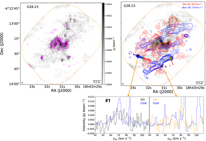
(b)

Figure 10: Presented here are individual plots for Figure 1 which are available as the online material. Dashed orange contour indicates 20% of the sensitivity level of the mosaic from the ALMA continuum image. The green stars indicate the identified dense cores. Upper left: ALMA 1.3 mm continuum image of G28.23. The contour levels are (-4, -3, 3, 4, 5, 6, 7, 8, 9)$\times\sigma$, with $\sigma=$0.164 mJy beam^-1. Upper right: The blue-shifted (blue contours) and red-shifted (red contours) components of CO emission, and SiO velocity-integrated intensity (black contours, integration range is between 67 and 85 km s^-1) overlaid on the continuum emission. The blue and red contours levels are (4, 6, 9, 13, 18, 24, 31, 39, 49, 60)$\times\sigma$, where the $\sigma$ are 0.035 Jy beam^-1 km s^-1 and 0.06 Jy beam^-1 km s^-1 for blue and red contours, respectively. The black contours are (3, 4, 5, 6, 7, 8, 9)$\times\sigma$, with $\sigma=$ 0.015 Jy beam^-1 km s^-1. Green stars show the position of the dust cores. On the left side panels, black numbers correspond to the name of all cores. On the right side panels, the green numbers indicate only the cores associated with molecular outflows. Bottom: example spectra of SiO and CO lines. The black vertical dashed lines represent the $v_{\rm lsr}$ of the clump.

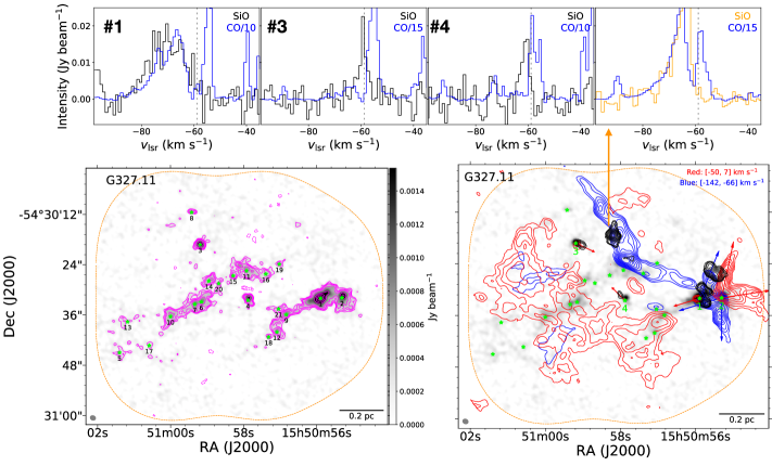
(c)

Figure 10: Presented here are individual plots for Figure 1 which are available as the online material. Dashed orange contour indicates 20% of the sensitivity level of the mosaic from the ALMA continuum image. The green stars indicate the identified dense cores. Upper: example spectra of SiO and CO lines. The black vertical dashed lines represent the $v_{\rm lsr}$ of the clump. Bottom left: ALMA 1.3 mm continuum image of G327.11. The contour levels are (-4, -3, 3, 4, 5, 7, 10, 15, 23, 35)$\times\sigma$, with $\sigma=$0.089 mJy beam^-1. Bottom right: The blue-shifted (blue contours) and red-shifted (red contours) components of CO emission, and SiO velocity-integrated intensity (black contours, integration range is between -68 and -58 km s^-1) overlaid on the continuum emission. The blue and red contours levels are (4, 6, 9, 13, 18, 24, 31, 39, 49, 60)$\times\sigma$, where the $\sigma$ are 0.04 Jy beam^-1 km s^-1 and 0.025 Jy beam^-1 km s^-1 for blue and red contours, respectively. The black contours are (3, 4, 5, 7, 10, 14, 19, 25)$\times\sigma$, with $\sigma=$ 0.01 Jy beam^-1 km s^-1. Green stars show the position of the dust cores. On the left side panels, black numbers correspond to the name of all cores. On the right side panels, the green numbers indicate only the cores associated with molecular outflows. The directions of outflow #1 and #2 toward #2–G327.11 are approximately along southeast-northwest and south-north, respectively.

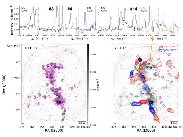
(d)

Figure 10: Presented here are individual plots for Figure 1 which are available as the online material. Dashed orange contour shows 20% of the sensitivity level of the mosaic from the ALMA continuum image. The green stars indicate the identified dense cores. Upper: example spectra of SiO and CO lines. The black vertical dashed lines represent the $v_{\rm lsr}$ of the clump. Bottom left: ALMA 1.3 mm continuum image of G331.37. The contour levels are (-4, -3, 3, 4, 5, 7, 9, 12, 16)$\times\sigma$, with $\sigma=$0.083 mJy beam^-1. Bottom right: The blue-shifted (blue contours) and red-shifted (red contours) components of CO emission, and SiO velocity-integrated intensity (black contours, integration range is between -95 and -69 km s^-1) overlaid on the continuum emission. The blue and red contours levels are (4, 6, 9, 13, 18, 24, 31, 39, 49, 60)$\times\sigma$, where the $\sigma$ are 0.025 Jy beam^-1 km s^-1 and 0.01 Jy beam^-1 km s^-1 for blue and red contours, respectively. The black contours are (3, 4, 5, 6, 7, 10, 14, 19, 25)$\times\sigma$, with $\sigma=$ 0.015 Jy beam^-1 km s^-1. Green stars show the position of the dust cores. On the left side panels, black numbers correspond to the name of all cores. On the right side panels, the green numbers indicate only the cores associated with molecular outflows.

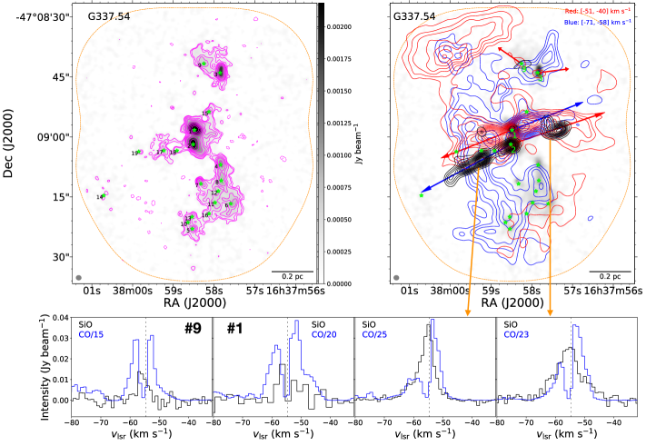
(e)

Figure 10: Presented here are individual plots for Figure 1 which are available as the online material. Dashed orange contour shows 20% of the sensitivity level of the mosaic from the ALMA continuum image. The green stars indicate the identified dense cores. Upper left: ALMA 1.3 mm continuum image of G337.54. The contour levels are (-4, -3, 3, 4, 6, 8, 10, 14, 20, 30, 45, 75)$\times\sigma$, with $\sigma=$0.068 mJy beam^-1. Upper right: The blue-shifted (blue contours) and red-shifted (red contours) components of CO emission, and SiO velocity-integrated intensity (black contours, integration range is between -67 and -45 km s^-1) overlaid on the continuum emission. The blue and red contours levels are (5, 7, 9, 14, 20, 27, 35, 44, 54, 74)$\times\sigma$, where the $\sigma$ are 0.08 Jy beam^-1 km s^-1 and 0.13 Jy beam^-1 km s^-1 for blue and red contours, respectively. The black contours are (3, 5, 6, 7, 9, 11, 13, 15, 17)$\times\sigma$, with $\sigma=$ 0.015 Jy beam^-1 km s^-1. Green stars show the position of the dust cores. On the left side panels, black numbers correspond to the name of all cores. On the right side panels, the green numbers indicate only the cores associated with molecular outflows. Bottom: example spectra of SiO and CO lines. The black vertical dashed lines represent the $v_{\rm lsr}$ of the clump.

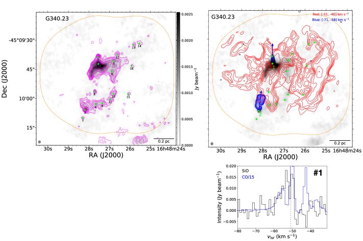
(f)

Figure 10: Presented here are individual plots for Figure 1 which are available as the online material. Dashed orange contour indicates 20% of the sensitivity level of the mosaic from the ALMA continuum image. The green stars indicate the identified dense cores. Upper left: ALMA 1.3 mm continuum image of G340.23. The contour levels are (-4, -3, 3, 4, 5, 7, 8, 11, 14, 18, 23)$\times\sigma$, with $\sigma=$0.139 mJy beam^-1. Upper right: The blue-shifted (blue contours) components of CO emission and SiO velocity-integrated intensity (black contours, integration range is between -60 and -47 km s^-1) overlaid on the continuum emission. The blue red contours levels are (5, 7, 9, 12, 15, 20, 31, 30, 40, 50)$\times\sigma$, where the $\sigma$ are 0.02 Jy beam^-1 km s^-1 for blue contours. The black contours are (3, 4, 5, 6, 7, 10, 14, 19, 25)$\times\sigma$, with $\sigma=$ 0.015 Jy beam^-1 km s^-1. Green stars show the position of the dust cores. On the left side panels, black numbers correspond to the name of all cores. On the right side panels, the green numbers indicate only the cores associated with molecular outflows. Bottom: example spectra of SiO and CO lines. The black vertical dashed lines represent the $v_{\rm lsr}$ of the clump.

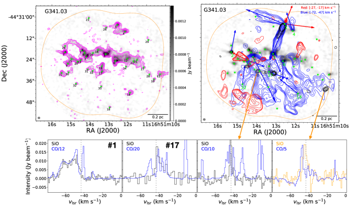
(g)

Figure 10: Presented here are individual plots for Figure 1 which are available as the online material. Dashed orange contour indicates 20% of the sensitivity level of the mosaic from the ALMA continuum image. The green stars indicate the identified dense cores. Upper left: ALMA 1.3 mm continuum image of G341.03. The contour levels are (-4, -3, 3, 4, 6, 9, 12, 16, 22)$\times\sigma$, with $\sigma=$0.070 mJy beam^-1. Upper right: The blue-shifted (blue contours) and red-shifted (red contours) components of CO emission, and SiO velocity-integrated intensity (black contours, integration range is between -66 and -31 km s^-1) overlaid on the continuum emission. The blue and red contours levels are (5, 7, 9, 14, 20, 27, 35, 44, 54, 74)$\times\sigma$, where the $\sigma$ are 0.07 Jy beam^-1 km s^-1 and 0.015 Jy beam^-1 km s^-1 for blue and red contours, respectively. The black contours are (3, 5, 6, 7, 9, 11, 13, 15, 17)$\times\sigma$, with $\sigma=$ 0.02 Jy beam^-1 km s^-1. Green stars show the position of the dust cores. On the left side panels, black numbers correspond to the name of all cores. On the right side panels, the green numbers indicate only the cores associated with molecular outflows. Bottom: example spectra of SiO and CO lines. The black vertical dashed lines represent the $v_{\rm lsr}$ of the clump. The directions of outflow #1 and #2 toward #1–G341.03 are approximately along northeast-southwest and southeast-northwest, respectively.

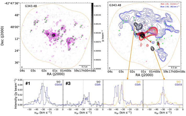
(h)

Figure 10: Presented here are individual plots for Figure 1 which are available as the online material. Dashed orange contour indicates 20% of the sensitivity level of the mosaic from the ALMA continuum image. The green stars indicate the identified dense cores. Upper left: ALMA 1.3 mm continuum image of G343.48. The contour levels are (-4, -3, 3, 4, 6, 8, 12, 20, 40, 100)$\times\sigma$, with $\sigma=$0.068 mJy beam^-1. Upper right: The blue-shifted (blue contours) and red-shifted (red contours) components of CO emission, and SiO velocity-integrated intensity (black contours, integration range is between -42 and -19 km s^-1) overlaid on the continuum emission. The blue and red contours levels are (5, 7, 9, 14, 20, 27, 35, 44, 54, 74)$\times\sigma$, where the $\sigma$ are 0.04 Jy beam^-1 km s^-1 and 0.06 Jy beam^-1 km s^-1 for blue and red contours, respectively. The black contours are (3, 4, 5, 6, 7, 9, 11, 14, 20, 27)$\times\sigma$, with $\sigma=$ 0.015 Jy beam^-1 km s^-1. Green stars show the position of the dust cores. On the left side panels, black numbers correspond to the name of all cores. On the right side panels, the green numbers indicate only the cores associated with molecular outflows. Bottom: example spectra of SiO and CO lines. The black vertical dashed lines represent the $v_{\rm lsr}$ of the clump.

References

- Alves et al. (2019) Alves, F. O., Caselli, P., Girart, J. M., et al. 2019, Science, 366, 90, doi: 10.1126/science.aaw3491
- Arce et al. (2010) Arce, H. G., Borkin, M. A., Goodman, A. A., Pineda, J. E., & Halle, M. W. 2010, ApJ, 715, 1170, doi: 10.1088/0004-637X/715/2/1170
- Arce & Goodman (2001) Arce, H. G., & Goodman, A. A. 2001, ApJ, 554, 132, doi: 10.1086/321334
- Arce et al. (2007) Arce, H. G., Shepherd, D., Gueth, F., et al. 2007, in Protostars and Planets V, ed. B. Reipurth, D. Jewitt, & K. Keil, 245. https://arxiv.org/abs/astro-ph/0603071
- Astropy Collaboration et al. (2013) Astropy Collaboration, Robitaille, T. P., Tollerud, E. J., et al. 2013, A&A, 558, A33, doi: 10.1051/0004-6361/201322068
- Audard et al. (2014) Audard, M., Ábrahám, P., Dunham, M. M., et al. 2014, in Protostars and Planets VI, ed. H. Beuther, R. S. Klessen, C. P. Dullemond, & T. Henning, 387, doi: 10.2458/azu_uapress_9780816531240-ch017
- Bachiller et al. (1991) Bachiller, R., Martin-Pintado, J., & Fuente, A. 1991, A&A, 243, L21
- Bally (2016) Bally, J. 2016, ARA&A, 54, 491, doi: 10.1146/annurev-astro-081915-023341
- Bally & Lada (1983) Bally, J., & Lada, C. J. 1983, ApJ, 265, 824, doi: 10.1086/160729
- Baug et al. (2020) Baug, T., Wang, K., Liu, T., et al. 2020, ApJ, 890, 44, doi: 10.3847/1538-4357/ab66b6
- Beltrán et al. (2006) Beltrán, M. T., Cesaroni, R., Codella, C., et al. 2006, Nature, 443, 427, doi: 10.1038/nature05074
- Beltrán & de Wit (2016) Beltrán, M. T., & de Wit, W. J. 2016, A&A Rev., 24, 6, doi: 10.1007/s00159-015-0089-z
- Beuther et al. (2002) Beuther, H., Schilke, P., Sridharan, T. K., et al. 2002, A&A, 383, 892, doi: 10.1051/0004-6361:20011808
- Blake et al. (1987) Blake, G. A., Sutton, E. C., Masson, C. R., & Phillips, T. G. 1987, ApJ, 315, 621, doi: 10.1086/165165
- Cabrit & Bertout (1992) Cabrit, S., & Bertout, C. 1992, A&A, 261, 274
- Caratti o Garatti et al. (2017) Caratti o Garatti, A., Stecklum, B., Garcia Lopez, R., et al. 2017, Nature Physics, 13, 276, doi: 10.1038/nphys3942
- Cesaroni et al. (2018) Cesaroni, R., Moscadelli, L., Neri, R., et al. 2018, A&A, 612, A103, doi: 10.1051/0004-6361/201732238
- Cheng et al. (2019) Cheng, Y., Qiu, K., Zhang, Q., et al. 2019, ApJ, 877, 112, doi: 10.3847/1538-4357/ab15d4
- Codella et al. (2013) Codella, C., Beltrán, M. T., Cesaroni, R., et al. 2013, A&A, 550, A81, doi: 10.1051/0004-6361/201219900
- Cody & Hillenbrand (2018) Cody, A. M., & Hillenbrand, L. A. 2018, AJ, 156, 71, doi: 10.3847/1538-3881/aacead
- Contreras et al. (2017) Contreras, Y., Rathborne, J. M., Guzman, A., et al. 2017, MNRAS, 466, 340, doi: 10.1093/mnras/stw3110
- Contreras et al. (2013) Contreras, Y., Schuller, F., Urquhart, J. S., et al. 2013, A&A, 549, A45, doi: 10.1051/0004-6361/201220155
- Contreras et al. (2018) Contreras, Y., Sanhueza, P., Jackson, J. M., et al. 2018, ApJ, 861, 14, doi: 10.3847/1538-4357/aac2ec
- Csengeri et al. (2011) Csengeri, T., Bontemps, S., Schneider, N., et al. 2011, ApJ, 740, L5, doi: 10.1088/2041-8205/740/1/L5
- Csengeri et al. (2016) Csengeri, T., Leurini, S., Wyrowski, F., et al. 2016, A&A, 586, A149, doi: 10.1051/0004-6361/201425404
- Cunningham et al. (2009) Cunningham, A. J., Frank, A., Carroll, J., Blackman, E. G., & Quillen, A. C. 2009, ApJ, 692, 816, doi: 10.1088/0004-637X/692/1/816
- Duarte-Cabral et al. (2014) Duarte-Cabral, A., Bontemps, S., Motte, F., et al. 2014, A&A, 570, A1, doi: 10.1051/0004-6361/201423677
- Duarte-Cabral et al. (2013) —. 2013, A&A, 558, A125, doi: 10.1051/0004-6361/201321393
- Dunham et al. (2014) Dunham, M. M., Arce, H. G., Mardones, D., et al. 2014, ApJ, 783, 29, doi: 10.1088/0004-637X/783/1/29
- Ellerbroek et al. (2013) Ellerbroek, L. E., Podio, L., Kaper, L., et al. 2013, A&A, 551, A5, doi: 10.1051/0004-6361/201220635
- Feddersen et al. (2020a) Feddersen, J. R., Arce, H. G., Kong, S., et al. 2020a, arXiv e-prints, arXiv:2004.03504. https://arxiv.org/abs/2004.03504
- Feddersen et al. (2020b) —. 2020b, ApJ, 896, 11, doi: 10.3847/1538-4357/ab86a9
- Federrath et al. (2014) Federrath, C., Schrön, M., Banerjee, R., & Klessen, R. S. 2014, ApJ, 790, 128, doi: 10.1088/0004-637X/790/2/128
- Fernández-López et al. (2013) Fernández-López, M., Girart, J. M., Curiel, S., et al. 2013, ApJ, 778, 72, doi: 10.1088/0004-637X/778/1/72
- Foster et al. (2011) Foster, J. B., Jackson, J. M., Barnes, P. J., et al. 2011, ApJS, 197, 25, doi: 10.1088/0067-0049/197/2/25
- Foster et al. (2013) Foster, J. B., Rathborne, J. M., Sanhueza, P., et al. 2013, PASA, 30, e038, doi: 10.1017/pasa.2013.18
- Foster et al. (2014) Foster, J. B., Arce, H. G., Kassis, M., et al. 2014, ApJ, 791, 108, doi: 10.1088/0004-637X/791/2/108
- Frank et al. (2014) Frank, A., Ray, T. P., Cabrit, S., et al. 2014, in Protostars and Planets VI, ed. H. Beuther, R. S. Klessen, C. P. Dullemond, & T. Henning, 451, doi: 10.2458/azu_uapress_9780816531240-ch020
- Graves et al. (2010) Graves, S. F., Richer, J. S., Buckle, J. V., et al. 2010, MNRAS, 409, 1412, doi: 10.1111/j.1365-2966.2010.17140.x
- Guzmán et al. (2015) Guzmán, A. E., Sanhueza, P., Contreras, Y., et al. 2015, ApJ, 815, 130, doi: 10.1088/0004-637X/815/2/130
- Hervías-Caimapo et al. (2019) Hervías-Caimapo, C., Merello, M., Bronfman, L., et al. 2019, ApJ, 872, 200, doi: 10.3847/1538-4357/aaf9ac
- Hirano et al. (2006) Hirano, N., Liu, S.-Y., Shang, H., et al. 2006, ApJ, 636, L141, doi: 10.1086/500201
- Hosokawa & Omukai (2009) Hosokawa, T., & Omukai, K. 2009, ApJ, 691, 823, doi: 10.1088/0004-637X/691/1/823
- Hunter (2007) Hunter, J. D. 2007, Computing in Science Engineering, 9, 90
- Hunter et al. (2017) Hunter, T. R., Brogan, C. L., MacLeod, G., et al. 2017, ApJ, 837, L29, doi: 10.3847/2041-8213/aa5d0e
- Jackson et al. (2013) Jackson, J. M., Rathborne, J. M., Foster, J. B., et al. 2013, PASA, 30, e057, doi: 10.1017/pasa.2013.37
- Jiménez-Serra et al. (2010) Jiménez-Serra, I., Caselli, P., Tan, J. C., et al. 2010, MNRAS, 406, 187, doi: 10.1111/j.1365-2966.2010.16698.x
- Joye & Mandel (2003) Joye, W. A., & Mandel, E. 2003, in Astronomical Society of the Pacific Conference Series, Vol. 295, Astronomical Data Analysis Software and Systems XII, ed. H. E. Payne, R. I. Jedrzejewski, & R. N. Hook, 489
- Keto (2003) Keto, E. 2003, ApJ, 599, 1196, doi: 10.1086/379545
- Keto et al. (1988) Keto, E. R., Ho, P. T. P., & Haschick, A. D. 1988, ApJ, 324, 920, doi: 10.1086/165949
- Kim & Kurtz (2006) Kim, K.-T., & Kurtz, S. E. 2006, ApJ, 643, 978, doi: 10.1086/502961
- Krumholz et al. (2009) Krumholz, M. R., Klein, R. I., McKee, C. F., Offner, S. S. R., & Cunningham, A. J. 2009, Science, 323, 754, doi: 10.1126/science.1165857
- Krumholz et al. (2014) Krumholz, M. R., Bate, M. R., Arce, H. G., et al. 2014, in Protostars and Planets VI, ed. H. Beuther, R. S. Klessen, C. P. Dullemond, & T. Henning, 243, doi: 10.2458/azu_uapress_9780816531240-ch011
- Kuiper et al. (2010) Kuiper, R., Klahr, H., Beuther, H., & Henning, T. 2010, ApJ, 722, 1556, doi: 10.1088/0004-637X/722/2/1556
- Kuiper et al. (2011) —. 2011, ApJ, 732, 20, doi: 10.1088/0004-637X/732/1/20
- Kuiper et al. (2016) Kuiper, R., Turner, N. J., & Yorke, H. W. 2016, ApJ, 832, 40, doi: 10.3847/0004-637X/832/1/40
- Kuiper et al. (2015) Kuiper, R., Yorke, H. W., & Turner, N. J. 2015, ApJ, 800, 86, doi: 10.1088/0004-637X/800/2/86
- Lada & Fich (1996) Lada, C. J., & Fich, M. 1996, ApJ, 459, 638, doi: 10.1086/176929
- Leurini et al. (2013) Leurini, S., Codella, C., Gusdorf, A., et al. 2013, A&A, 554, A35, doi: 10.1051/0004-6361/201118154
- Leurini et al. (2014) Leurini, S., Codella, C., López-Sepulcre, A., et al. 2014, A&A, 570, A49, doi: 10.1051/0004-6361/201424251
- Li et al. (2015) Li, H., Li, D., Qian, L., et al. 2015, ApJS, 219, 20, doi: 10.1088/0067-0049/219/2/20
- Li et al. (2019a) Li, S., Zhang, Q., Pillai, T., et al. 2019a, ApJ, 886, 130, doi: 10.3847/1538-4357/ab464e
- Li et al. (2017) Li, S., Wang, J., Zhang, Z.-Y., et al. 2017, MNRAS, 466, 248, doi: 10.1093/mnras/stw3076
- Li et al. (2019b) Li, S., Wang, J., Fang, M., et al. 2019b, ApJ, 878, 29, doi: 10.3847/1538-4357/ab1e4c
- Li & Nakamura (2006) Li, Z.-Y., & Nakamura, F. 2006, ApJ, 640, L187, doi: 10.1086/503419
- Liu et al. (2017) Liu, T., Lacy, J., Li, P. S., et al. 2017, ApJ, 849, 25, doi: 10.3847/1538-4357/aa8d73
- Lodato & Clarke (2004) Lodato, G., & Clarke, C. J. 2004, MNRAS, 353, 841, doi: 10.1111/j.1365-2966.2004.08112.x
- López-Sepulcre et al. (2010) López-Sepulcre, A., Cesaroni, R., & Walmsley, C. M. 2010, A&A, 517, A66, doi: 10.1051/0004-6361/201014252
- Lu et al. (2015) Lu, X., Zhang, Q., Wang, K., & Gu, Q. 2015, ApJ, 805, 171, doi: 10.1088/0004-637X/805/2/171
- Lu et al. (2018) Lu, X., Zhang, Q., Liu, H. B., et al. 2018, ApJ, 855, 9, doi: 10.3847/1538-4357/aaad11
- Mac Low (1999) Mac Low, M.-M. 1999, ApJ, 524, 169, doi: 10.1086/307784
- Mangum & Shirley (2015) Mangum, J. G., & Shirley, Y. L. 2015, PASP, 127, 266, doi: 10.1086/680323
- McKee & Ostriker (2007) McKee, C. F., & Ostriker, E. C. 2007, ARA&A, 45, 565, doi: 10.1146/annurev.astro.45.051806.110602
- McKee & Tan (2003) McKee, C. F., & Tan, J. C. 2003, ApJ, 585, 850, doi: 10.1086/346149
- McMullin et al. (2007) McMullin, J. P., Waters, B., Schiebel, D., Young, W., & Golap, K. 2007, in Astronomical Society of the Pacific Conference Series, Vol. 376, Astronomical Data Analysis Software and Systems XVI, ed. R. A. Shaw, F. Hill, & D. J. Bell, 127
- Molinari et al. (2008) Molinari, S., Pezzuto, S., Cesaroni, R., et al. 2008, A&A, 481, 345, doi: 10.1051/0004-6361:20078661
- Nakamura & Li (2007) Nakamura, F., & Li, Z.-Y. 2007, ApJ, 662, 395, doi: 10.1086/517515
- Nakamura & Li (2014) —. 2014, ApJ, 783, 115, doi: 10.1088/0004-637X/783/2/115
- Nakamura et al. (2011a) Nakamura, F., Sugitani, K., Shimajiri, Y., et al. 2011a, ApJ, 737, 56, doi: 10.1088/0004-637X/737/2/56
- Nakamura et al. (2011b) Nakamura, F., Kamada, Y., Kamazaki, T., et al. 2011b, ApJ, 726, 46, doi: 10.1088/0004-637X/726/1/46
- Nony et al. (2020) Nony, T., Motte, F., Louvet, F., et al. 2020, A&A, 636, A38, doi: 10.1051/0004-6361/201937046
- Offner & Chaban (2017) Offner, S. S. R., & Chaban, J. 2017, ApJ, 847, 104, doi: 10.3847/1538-4357/aa8996
- Offner & Liu (2018) Offner, S. S. R., & Liu, Y. 2018, Nature Astronomy, 2, 896, doi: 10.1038/s41550-018-0566-1
- Palau et al. (2006) Palau, A., Ho, P. T. P., Zhang, Q., et al. 2006, ApJ, 636, L137, doi: 10.1086/500242
- Parks et al. (2014) Parks, J. R., Plavchan, P., White, R. J., & Gee, A. H. 2014, ApJS, 211, 3, doi: 10.1088/0067-0049/211/1/3
- Pillai et al. (2019) Pillai, T., Kauffmann, J., Zhang, Q., et al. 2019, A&A, 622, A54, doi: 10.1051/0004-6361/201732570
- Plunkett et al. (2015a) Plunkett, A. L., Arce, H. G., Corder, S. A., et al. 2015a, ApJ, 803, 22, doi: 10.1088/0004-637X/803/1/22
- Plunkett et al. (2015b) Plunkett, A. L., Arce, H. G., Mardones, D., et al. 2015b, Nature, 527, 70, doi: 10.1038/nature15702
- Pudritz & Norman (1983) Pudritz, R. E., & Norman, C. A. 1983, ApJ, 274, 677, doi: 10.1086/161481
- Pudritz & Norman (1986) —. 1986, ApJ, 301, 571, doi: 10.1086/163924
- Qiu et al. (2019) Qiu, K., Wyrowski, F., Menten, K., Zhang, Q., & Güsten, R. 2019, ApJ, 871, 141, doi: 10.3847/1538-4357/aaf728
- Qiu & Zhang (2009) Qiu, K., & Zhang, Q. 2009, ApJ, 702, L66, doi: 10.1088/0004-637X/702/1/L66
- Qiu et al. (2009) Qiu, K., Zhang, Q., Wu, J., & Chen, H.-R. 2009, ApJ, 696, 66, doi: 10.1088/0004-637X/696/1/66
- Qiu et al. (2008) Qiu, K., Zhang, Q., Megeath, S. T., et al. 2008, ApJ, 685, 1005, doi: 10.1086/591044
- Rathborne et al. (2016) Rathborne, J. M., Whitaker, J. S., Jackson, J. M., et al. 2016, PASA, 33, e030, doi: 10.1017/pasa.2016.23
- Richer et al. (2000) Richer, J. S., Shepherd, D. S., Cabrit, S., Bachiller, R., & Churchwell, E. 2000, Protostars and Planets IV, 867
- Robitaille & Bressert (2012) Robitaille, T., & Bressert, E. 2012, APLpy: Astronomical Plotting Library in Python, Astrophysics Source Code Library. http://ascl.net/1208.017
- Rohde et al. (2019) Rohde, P. F., Walch, S., Seifried, D., et al. 2019, MNRAS, 483, 2563, doi: 10.1093/mnras/sty3302
- Sakai et al. (2013) Sakai, T., Sakai, N., Foster, J. B., et al. 2013, ApJ, 775, L31, doi: 10.1088/2041-8205/775/1/L31
- Sanhueza et al. (2010) Sanhueza, P., Garay, G., Bronfman, L., et al. 2010, ApJ, 715, 18, doi: 10.1088/0004-637X/715/1/18
- Sanhueza et al. (2012) Sanhueza, P., Jackson, J. M., Foster, J. B., et al. 2012, ApJ, 756, 60, doi: 10.1088/0004-637X/756/1/60
- Sanhueza et al. (2013) —. 2013, ApJ, 773, 123, doi: 10.1088/0004-637X/773/2/123
- Sanhueza et al. (2017) Sanhueza, P., Jackson, J. M., Zhang, Q., et al. 2017, ApJ, 841, 97, doi: 10.3847/1538-4357/aa6ff8
- Sanhueza et al. (2019) Sanhueza, P., Contreras, Y., Wu, B., et al. 2019, ApJ, 886, 102, doi: 10.3847/1538-4357/ab45e9
- Santiago-García et al. (2009) Santiago-García, J., Tafalla, M., Johnstone, D., & Bachiller, R. 2009, A&A, 495, 169, doi: 10.1051/0004-6361:200810739
- Schilke et al. (1997) Schilke, P., Walmsley, C. M., Pineau des Forets, G., & Flower, D. R. 1997, A&A, 321, 293
- Scholz et al. (2013) Scholz, A., Froebrich, D., & Wood, K. 2013, MNRAS, 430, 2910, doi: 10.1093/mnras/stt091
- Schuller et al. (2009) Schuller, F., Menten, K. M., Contreras, Y., et al. 2009, A&A, 504, 415, doi: 10.1051/0004-6361/200811568
- Shang et al. (2007) Shang, H., Li, Z. Y., & Hirano, N. 2007, in Protostars and Planets V, ed. B. Reipurth, D. Jewitt, & K. Keil, 261
- Sheikhnezami et al. (2012) Sheikhnezami, S., Fendt, C., Porth, O., Vaidya, B., & Ghanbari, J. 2012, ApJ, 757, 65, doi: 10.1088/0004-637X/757/1/65
- Shu et al. (1987) Shu, F. H., Adams, F. C., & Lizano, S. 1987, ARA&A, 25, 23, doi: 10.1146/annurev.aa.25.090187.000323
- Shu et al. (2000) Shu, F. H., Najita, J. R., Shang, H., & Li, Z.-Y. 2000, Protostars and Planets IV, 789
- Shu et al. (1991) Shu, F. H., Ruden, S. P., Lada, C. J., & Lizano, S. 1991, ApJ, 370, L31, doi: 10.1086/185970
- Stephens et al. (2015) Stephens, I. W., Jackson, J. M., Sanhueza, P., et al. 2015, ApJ, 802, 6, doi: 10.1088/0004-637X/802/1/6
- Tomisaka (1998) Tomisaka, K. 1998, ApJ, 502, L163, doi: 10.1086/311504
- van Kempen et al. (2016) van Kempen, T. A., Hogerheijde, M. R., van Dishoeck, E. F., et al. 2016, A&A, 587, A17, doi: 10.1051/0004-6361/201424725
- Vorobyov & Basu (2010) Vorobyov, E. I., & Basu, S. 2010, ApJ, 719, 1896, doi: 10.1088/0004-637X/719/2/1896
- Vorobyov et al. (2018) Vorobyov, E. I., Elbakyan, V. G., Plunkett, A. L., et al. 2018, A&A, 613, A18, doi: 10.1051/0004-6361/201732253
- Wang et al. (2011) Wang, K., Zhang, Q., Wu, Y., & Zhang, H. 2011, ApJ, 735, 64, doi: 10.1088/0004-637X/735/1/64
- Wang et al. (2010) Wang, P., Li, Z.-Y., Abel, T., & Nakamura, F. 2010, ApJ, 709, 27, doi: 10.1088/0004-637X/709/1/27
- Whitaker et al. (2017) Whitaker, J. S., Jackson, J. M., Rathborne, J. M., et al. 2017, AJ, 154, 140, doi: 10.3847/1538-3881/aa86ad
- Wyrowski et al. (2016) Wyrowski, F., Güsten, R., Menten, K. M., et al. 2016, A&A, 585, A149, doi: 10.1051/0004-6361/201526361
- Yang et al. (2018) Yang, A. Y., Thompson, M. A., Urquhart, J. S., & Tian, W. W. 2018, ApJS, 235, 3, doi: 10.3847/1538-4365/aaa297
- Zhang & Ho (1997) Zhang, Q., & Ho, P. T. P. 1997, ApJ, 488, 241, doi: 10.1086/304667
- Zhang et al. (2000) Zhang, Q., Ho, P. T. P., & Wright, M. C. H. 2000, AJ, 119, 1345, doi: 10.1086/301274
- Zhang et al. (2005) Zhang, Q., Hunter, T. R., Brand, J., et al. 2005, ApJ, 625, 864, doi: 10.1086/429660
- Zhang et al. (2001) —. 2001, ApJ, 552, L167, doi: 10.1086/320345
- Zhang et al. (1999) Zhang, Q., Hunter, T. R., Sridharan, T. K., & Cesaroni, R. 1999, ApJ, 527, L117, doi: 10.1086/312411
- Zhang et al. (2015) Zhang, Q., Wang, K., Lu, X., & Jiménez-Serra, I. 2015, ApJ, 804, 141, doi: 10.1088/0004-637X/804/2/141
- Zhu et al. (2009) Zhu, Z., Hartmann, L., & Gammie, C. 2009, ApJ, 694, 1045, doi: 10.1088/0004-637X/694/2/1045