Jet Marching Methods for Solving the Eikonal Equation

Abstract

We develop a family of compact high-order semi-Lagrangian label-setting methods for solving the eikonal equation. These solvers march the total 1-jet of the eikonal, and use Hermite interpolation to approximate the eikonal and parametrize characteristics locally for each semi-Lagrangian update. We describe solvers on unstructured meshes in any dimension, and conduct numerical experiments on regular grids in two dimensions. Our results show that these solvers yield at least second-order convergence, and, in special cases such as a linear speed of sound, third-order of convergence for both the eikonal and its gradient. We additionally show how to march the second partials of the eikonal using cell-based interpolants. Second derivative information computed this way is frequently second-order accurate, suitable for locally solving the transport equation. This provides a means of marching the prefactor coming from the WKB approximation of the Helmholtz equation. These solvers are designed specifically for computing a high-frequency approximation of the Helmholtz equation in a complicated environment with a slowly varying speed of sound, and, to the best of our knowledge, are the first solvers with these properties. We provide a link to a package online providing the solvers, and from which the results of this paper can be reproduced easily.

65N99, 65Y20, 49M99

1 Introduction

Our goal is to develop a family of high-order semi-Lagrangian eikonal solvers which use compact stencils. This is motivated by problems in high-frequency room acoustics, although the eikonal equation arises in a tremendous variety of modeling problems [40].

In multimedia, virtual reality, and video games, precomputing room impulse responses (RIRs) or transfer functions (RTFs) enables convincing spatialized audio, in combination with binaural or surround sound formats. Such an approach, usually referred to as numerical acoustics, involves computing pairs of RIRs by placing probes at different locations in a voxelized domain, numerically solving the acoustic wave equation, and capturing salient perceptual parameters throughout the domain using a streaming encoder [33, 34]. These parameters are later decoded using signal processing techniques in real time as the listener moves throughout the virtual environment. Assuming that the encoded parameters can comfortably fit into memory, a drawback of this approach is that the complexity of the simulation depends intrinsically on the highest frequency simulated. In practice, simulations top out at around 1 kHz. The hearing range of humans is roughly 20 Hz to 20 kHz, which requires these methods to either implicitly or explicitly extrapolate the bandlimited transfer functions to the full audible spectrum.

An established alternative to this approach is geometric acoustics, where methods based on raytracing are used [35]. Contrary to methods familiar from computer graphics, the focus of geometric acoustics is different. Acoustic waves are mechanical and have macroscopic wavelengths. This means that subsurface scattering, typically modeled using BRDFs in raytracing for computer graphics [27], is less relevant, and is limited to modeling macroscopic scattering from small geometric features, since reflections from flat surfaces are specular in nature. What’s more, accurately modeling diffraction effects is crucial [36]: e.g., we can hear a sound source occluded by an obstacle, but we can’t see it. A variety of other geometric-acoustic methods exist beyond raytracing. Examples include the image source method [2] and frustum tracing [13].

Geometric acoustics and optics both assume a solution to the wave equation based on an asymptotic high-frequency (WKB) approximation to the Helmholtz equation [29]. In this approximation, the eikonal plays the role of a spatially varying phase function, whose level sets describe propagating wavefronts. The prefactor of this approximation describes the amplitude of these wavefronts. The WKB approximation assumes a ray of “infinite frequency”, suitable for optics, since the effects of diffraction are limited. A variety of mechanisms for augmenting this approximation with frequency-dependent diffraction effects have been proposed, the most successful of which is Keller’s geometric theory of diffraction [21] (including the later uniform theory of diffraction [23]).

The complete geometric acoustic field of multiply reflected and diffracted rays can be parametrized by repeatedly solving the eikonal equation, using boundary conditions derived from the WKB approximation to patch together successive fields. A related approach is Benamou’s big raytracing (BRT) [5, 6]. This approach requires one to be able to accurately solve the transport equation describing the amplitude, e.g. using paraxial raytracing [29]. In order to do this, the first and second order partial derivatives of the eikonal must be computed. High-order accurate iterative schemes for solving the eikonal equation exist [50, 48, 24], but their performance deteriorates in the presence of complicated obstacles. Direct solvers for the eikonal equation allow one to locally parametrize the characteristics (rays) of the eikonal equation, which puts one in a position to simultaneously march the amplitude. This enables work-efficient algorithms, critical if a large number of eikonal problems must be solved.

Benamou’s line of research related to BRT seems to have stalled due to difficulties faced with caustics [7]. This is reasonable considering that the intended use was seismic modeling, where the eikonal equation is used to model first arrival times of $P$-waves. In this case, the speed of sound is extremely complicated, resulting in a large number of caustics [47]. On the other hand, in room acoustics, the speed of sound varies slowly. The main challenge is geometric: the domain is potentially filled with obstacles. This provides another motivation for compact stencils: such stencils can be adapted for use with unstructured meshes, and the sort of complicated boundary conditions that arise when using finite differences are avoided entirely. In this work, our goal is to develop the underlying approach to obtaining a compact higher-order semi-Lagrangian eikonal solver. In future work, this will be applied in the unstructured setting.

The solvers developed in this work are high-order, have optimally local/compact stencils, and are label-setting methods (much like Sethian’s fast marching method [39] or Tsitsiklis’s semi-Lagrangian algorithm for solving the eikonal equation [46]). Additionally, being semi-Lagrangian, they locally parametrize characteristics (acoustic rays), making them suitable for use with paraxial raytracing [29], the method of choice for locally computing the amplitude. To the best of our knowledge, these are the first eikonal solvers with this collection of properties.

We refer to our solvers as jet marching methods to reflect the fact that the key idea is marching the jet of the eikonal (the eikonal and its partial derivatives up to a particular order [43]) in a principled fashion. Sethian and Vladimirsky developed a fast marching method that additionally marched the gradient of the eikonal in a short note, but did not prove convergence results or provide detailed numerical experiments [41]. Benamou and collaborators built on these ideas by exploiting information about the eikonal equation to obtain a compact upwind second-order finite difference scheme for solving the eikonal equation [8]. Related methods exist in the level set method community and are referred to as gradient-augmented level set methods or jet schemes [25, 37].

In the rest of this work we lay out these methods, providing detailed numerical experiments. Our presentation is for unstructured grids in $n$-dimensions, while our numerical experiments were carried out in 2D. We plan to extend these solvers to structured and unstructured meshes in 3D and will report on these later in the context of room acoustics applications.

1.1 Problem setup

Let $\Omega\subseteq\mathbb{R}^{n}$ be a domain, let $\partial\Omega$ be its boundary, and let $\Gamma\subseteq\Omega$. The eikonal equation is a nonlinear first-order hyperbolic partial differential equation given by:

(1) $$\begin{split}\|\nabla\tau(\boldsymbol{x})\|&=s(\boldsymbol{x}),\qquad\boldsymbol{x}\in\Omega,\\ \tau(\boldsymbol{x})&=g(\boldsymbol{x}),\qquad\boldsymbol{x}\in\Gamma.\end{split}$$

Here, $\tau:\Omega\to\mathbb{R}$ is the eikonal, a spatial phase function that encodes the first arrival time of a wavefront propagating with pointwise slowness specified by $s:\Omega\to(0,\infty)$, which can be thought of as an index of refraction. The function $g:\Gamma\to\mathbb{R}$ specifies the boundary conditions, and is subject to certain compatibility conditions [9].

One way of arriving at the eikonal equation is by approximating the solution $u$ of the Helmholtz equation:

(2) $$\Big{(}\Delta+\omega^{2}s(\boldsymbol{x})^{2}\Big{)}u(\boldsymbol{x})=0,$$

with the WKB ansatz:

(3) $$u(\boldsymbol{x})\sim\alpha(\boldsymbol{x})e^{i\omega\tau(\boldsymbol{x})},$$

where $\omega$ is the frequency [29]. As $\omega\to\infty$, this asymptotic approximation is $O(\omega^{-1})$ accurate. This is referred to as the geometric optics approximation [7]. The level sets of $\tau$ denote the arrival times of bundles of rays, and the amplitude $\alpha$, which satisfies the transport equation:

(4) $$\alpha(\boldsymbol{x})\Delta\tau(\boldsymbol{x})+2\nabla\tau(\boldsymbol{x})^{\top}\nabla\alpha(\boldsymbol{x})=0,$$

describes the attenuation of the amplitude of the wavefront due to the propagation and geometric spreading of rays. The characteristics (rays) of the eikonal equation satisfy the raytracing ODEs.

The solution of the eikonal equation is given by Fermat’s principle:

(5) $$\tau(\boldsymbol{x})=\min_{\begin{subarray}{c}\boldsymbol{y}\in\Gamma\\ \boldsymbol{\psi}:[0,1]\to\Omega\\ \boldsymbol{\psi}(0)=\boldsymbol{y},\boldsymbol{\psi}(1)=\boldsymbol{x}\end{subarray}}\left\{\tau(\boldsymbol{y})+\int_{0}^{1}s(\boldsymbol{\psi}(\sigma))\|\boldsymbol{\psi}^{\prime}(\sigma)\|d\sigma\right\}.$$

Observe that this equation is recursive, suggesting a connection with dynamic programming and Bellman’s principle of optimality. Indeed, the path $\boldsymbol{\psi}$ is a ray whose Lagrangian and Hamiltonian are:

(6) $$\mathcal{H}(\boldsymbol{x},\nabla\tau(\boldsymbol{x}))=\frac{\|\nabla\tau(\boldsymbol{x})\|^{2}-s(\boldsymbol{x})^{2}}{2}=0,\qquad\mathcal{L}(\boldsymbol{x},\dot{\boldsymbol{x}})=s(\boldsymbol{x})\|\dot{\boldsymbol{x}}\|.$$

This provides the connection between the Eulerian perspective given by the eikonal equation, Fermat’s principle, and the Lagrangian view provided by raytracing.

2 Related work

The quintessential numerical method for solving the eikonal equation is the fast marching method [38]. We discretize $\Omega$ into a grid of nodes $\Omega_{h}$, where $h>0$ is the characteristic length scale of elements in $\Omega_{h}$. Let $T:\Omega_{h}\to\mathbb{R}$ be the numerical eikonal. To compute $T$, equation (1) is discretized using first-order finite differences and the order in which individual values of $T$ are relaxed is determined using a variation of Dijkstra’s algorithm for solving the single source shortest paths problem [39, 40]. If $N=|\Omega_{h}|$, then the fast marching method solves (1) in $O(N\log N)$ with $O(h\log\tfrac{1}{h})$ worst-case accuracy [51]. The logarithmic factor only appears when rarefaction fans are present: e.g., point source boundary data, or if the wavefront diffracts around a singular corner or edge. In these cases, full $O(h)$ accuracy can be recovered by proper initialization near rarefaction fans, or by employing a variety of factoring schemes [17, 24, 31].

It is also possible to solve the eikonal equation using semi-Lagrangian numerical methods, in which the ansatz (5) is discretized and applied locally [46, 30]. For instance, at a point $\hat{\boldsymbol{x}}\in\Omega_{h}$, we consider a neighborhood of points $\texttt{nb}(\boldsymbol{x})\subseteq\Omega_{h}$, assume that $\tau$ is fixed over the “surface” of this neighborhood, and approximate (5). As an example, if $\texttt{nb}(\hat{\boldsymbol{x}})$ consists of its $2n$ nearest neighbors, if we linearly interpolate $\tau$ over the facets of $\operatorname{conv}(\texttt{nb}(\hat{\boldsymbol{x}}))$, and discretize the integral in (5) using a right-hand rule, the resulting solver is equivalent to the fast marching method [42].

The Eulerian approach has generally been favored when developing higher-order solvers for the eikonal equation [50]. The eikonal equation is discretized using higher-order finite difference schemes and solved in the same manner as the fast marching method or using a variety of appropriate iterative schemes. Unfortunately, these approaches presuppose a regular grid and require wide stencils.

Our goal is to develop solvers for the eikonal equation that are high order, are optimally local (only use information from the nodes in $\texttt{nb}(\hat{\boldsymbol{x}})$ to update $\hat{\boldsymbol{x}}$), and are flexible enough to work on unstructured meshes. Using a semi-Lagrangian approach based on a high-order discretization of (5) allows us to do this.

This work was inspired by several lines of research. First, are gradient-augmented level set methods (or jet schemes) [25, 37]. Although developed for solving time-dependent advection problems, trying to map ideas from the time-dependent to static setting is natural, and presented an intriguing challenge. Second, the idea of using a semi-Lagrangian solver to construct a finite element solution to the eikonal equation incrementally was informative [9]; while the authors only constructed a first-order finte element approximation, attempting to push past this formulation to obtain a higher-order solver is a natural extension. Third, we were motivated by Chopp’s idea of building up piecewise bicubic interpolants locally while marching the eikonal [14]; indeed, Chopp’s work is mentioned in the original work on jet schemes in a similar capacity.

3 The jet marching method

Label-setting algorithms [12], such as the fast marching method, compute an approximation to $\tau$ by marching a numerical approximation $T:\Omega_{h}\to\mathbb{R}^{n}$ throughout the domain. The boundary data $g$ is not always specified at the nodes of $\Omega_{h}$. Let $\Gamma_{h}$ be a discrete approximation of $\Gamma$. Once $T$ is computed at $\Gamma_{h}\subseteq\Omega_{h}$ with sufficiently high accuracy, the solver begins to operate. To drive the solver, a set of states $\{\texttt{far},\texttt{trial},\texttt{valid}\}$ is used for bookkeeping. We initially set:

(7) $$\texttt{state}(\boldsymbol{x})=\begin{cases}\texttt{trial},&\mbox{if }\boldsymbol{x}\in\Gamma_{h},\\ \texttt{far},&\mbox{otherwise.}\end{cases}$$

The trial nodes are typically sorted by their $T$ value into an array-based binary heap implementing a priority queue, although alternatives have been explored [18]. At each step of the iteration, the node $\boldsymbol{x}$ with the minimum $T$ value is removed from the heap, $\texttt{state}(\boldsymbol{x})$ is set to valid, the far nodes in $\texttt{nb}(\boldsymbol{x})$ have their state set to trial, and each trial node in $\texttt{nb}(\boldsymbol{x})$ is subsequently updated. We have additionally provided a video online which shows the algorithm running [11].

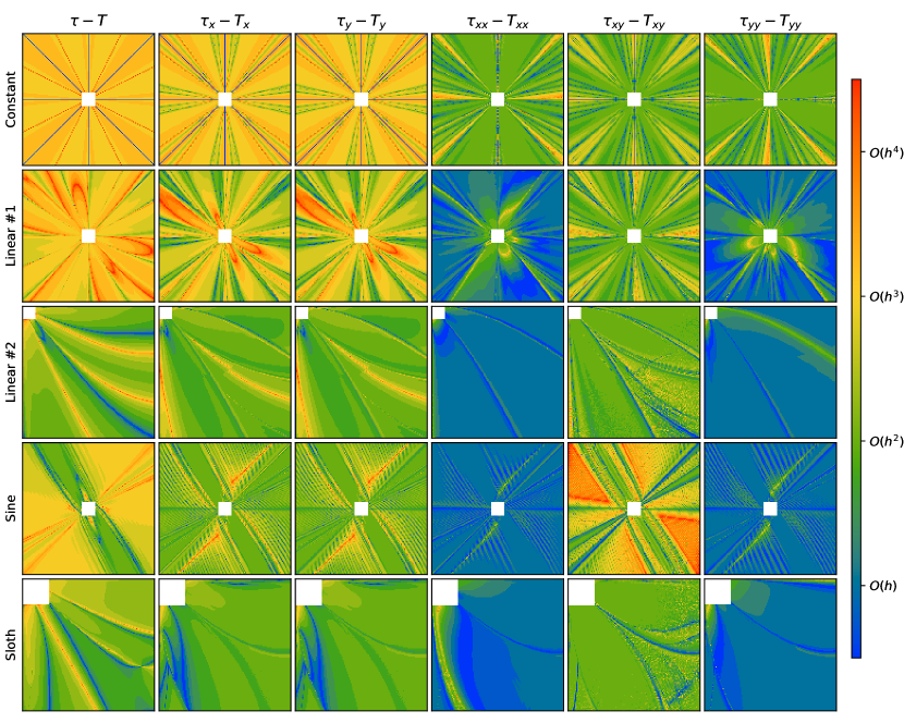
Figure 10: A plot of the pointwise convergence at each point in $\Omega_{h}$ for JMM4. To obtain these plots, starting with $N=129$, we decimate each larger problem size (up to $N=2,049$) to a $129\times 129$ grid, and do a least squares fit at each point. This gives us an estimate of the order of convergence at each point.

From this, we can see that the value $T(\boldsymbol{x})$ depends on the values of $T$ at the nodes of a directed graph leading from $\boldsymbol{x}$ back to $\Gamma_{h}$, noting that $T(\boldsymbol{x})$ can—and in general does—depend on multiple nodes in $\texttt{nb}(\boldsymbol{x})$. This means that the error in $T$ accumulates as the solution propagates downwind from $\Gamma_{h}$. We generally assume that the depth of the directed graph of updates connecting each $\boldsymbol{x}\in\Omega_{h}$ to $\Gamma_{h}$ is $O(h^{-1})$. The error due to each update comes from two sources: the running error accumulated in $T$, and the error incurred by approximating the integral in (5). For this reason, we would expect the order of the global error of the solver to be one less than the local error. However, the situation is more delicate because of the complicated manner in which the errors mix (see Figure 10). Our numerical results in Section 8 indicate that $T$ converges with between $O(h^{2})$ and $O(h^{3})$ accuracy, and $\nabla T$ converges with anywhere between $O(h)$ and $O(h^{3})$ accuracy.

Regardless, we assume that we only know the values of the eikonal and some of its derivatives at the nodes $\boldsymbol{x}\in\Omega_{h}$. To obtain higher-order accuracy locally, we make use of piecewise Hermite elements. In particular, at each node $\boldsymbol{x}$, we approximate the jet of the eikonal; i.e., $\tau$ and a number of its derivatives [43]. If we compute the jet with sufficiently high accuracy when we set $\texttt{state}(\boldsymbol{x})\leftarrow\texttt{valid}$, we will be in a position to approximate $\tau$ using Hermite interpolation locally over $\operatorname{conv}(\boldsymbol{x}_{1},\ldots,\boldsymbol{x}_{n})$. We consider several variations on this idea.

3.1 The general cost function

Fix a point $\hat{\boldsymbol{x}}\in\Omega_{h}$, thinking of it as the update point. To compute $T(\hat{\boldsymbol{x}})$, we consider sets of valid nodes $\{\boldsymbol{x}_{1},\ldots,\boldsymbol{x}_{d}\}\subseteq\texttt{nb}(\hat{\boldsymbol{x}})$, where $1\leq d\leq n$. The tuple of nodes $(\hat{\boldsymbol{x}},\boldsymbol{x}_{1},\ldots,\boldsymbol{x}_{d})$ is an update of dimension $d$, and the collection of updates a stencil. We refer to the nodes $\{\boldsymbol{x}_{1},\ldots,\boldsymbol{x}_{d}\}$ as the vertices of the base of the update. In some cases, such as on an unstructured mesh, stencils may vary with $\hat{\boldsymbol{x}}$. Sufficient conditions for the updates and stencils to be monotone causal have been studied [22]. In particular, the cone spanned by $\{\boldsymbol{x}_{1}-\hat{\boldsymbol{x}},\ldots,\boldsymbol{x}_{n}-\hat{\boldsymbol{x}}\}$ should fit inside the nonnegative orthant after being rotated [41, 42]. This is easily satisfied on a regular grid. For $O(h)$ solvers that do not make use of gradient information, a variety of choices of stencils are monotone causal.

To describe a general update, without loss of generality we assume $d=n$, and assume that the update nodes are in general position. That is, if we choose $n$ nodes from $\{\hat{\boldsymbol{x}},\boldsymbol{x}_{1},\ldots,\boldsymbol{x}_{n}\}$, the remaining node does not lie in their convex hull. We assume that we have access to a sufficiently accurate approximation of $\tau$ over $\operatorname{conv}(\boldsymbol{x}_{1},\ldots,\boldsymbol{x}_{n})$, call it $\mathsf{T}$. We distinguish between $\mathsf{T}$ and $T$ in the following way: $\mathsf{T}$ denotes the local numerical approximation of $\tau$ used by a particular update, while $T$ denotes the global numerical approximation of $\tau$. The two may not be equal to each other. Indeed, $T$ is in general only defined on $\Omega_{h}$, while $\mathsf{T}$ is only defined on $\operatorname{conv}(\boldsymbol{x}_{1},\ldots,\boldsymbol{x}_{n})$.

Let $\boldsymbol{x}_{\boldsymbol{\lambda}}\in\operatorname{conv}(\boldsymbol{x}_{1},\ldots,\boldsymbol{x}_{n})$, and let $L=L_{\boldsymbol{\lambda}}=\|\hat{\boldsymbol{x}}-\boldsymbol{x}_{\boldsymbol{\lambda}}\|$. Recall that $\boldsymbol{\psi}:[0,L]\to\Omega$ is the curve minimizing (5) for a particular choice of $\boldsymbol{x}_{\boldsymbol{\lambda}}$. We approximate $\boldsymbol{\psi}$ with a cubic parametric curve $\boldsymbol{\varphi}:[0,L]\to\Omega$ such that:

(8) $$\boldsymbol{\varphi}(0)=\boldsymbol{x}_{\boldsymbol{\lambda}},\qquad\boldsymbol{\varphi}(L)=\hat{\boldsymbol{x}},\qquad\boldsymbol{\varphi}^{\prime}(0)\sim\boldsymbol{t}_{\boldsymbol{\lambda}},\qquad\boldsymbol{\varphi}^{\prime}(L)\sim\hat{\boldsymbol{t}},$$

and where $\boldsymbol{t}_{\boldsymbol{\lambda}}$ and $\hat{\boldsymbol{t}}$ are tangent vectors which enter as parameters. Note that $\boldsymbol{\varphi}^{\prime}(0)$ and $\boldsymbol{\varphi}^{\prime}(L)$ may not be exactly equal to $\boldsymbol{t}_{\boldsymbol{\lambda}}$ and $\hat{\boldsymbol{t}}$.

We approximate the integral in (5) over $\boldsymbol{\varphi}$ using Simpson’s rule. This gives the cost functional:

(9) $$F(\boldsymbol{\varphi})=\mathsf{T}(\boldsymbol{x}_{\boldsymbol{\lambda}})+\frac{L}{6}\Big{[}s(\boldsymbol{x}_{\boldsymbol{\lambda}})\|\boldsymbol{\varphi}^{\prime}(0)\|+4s\big{(}\boldsymbol{\varphi}_{1/2}\big{)}\big{\|}\boldsymbol{\varphi}^{\prime}_{1/2}\big{\|}+s(\hat{\boldsymbol{x}})\|\boldsymbol{\varphi}^{\prime}(L)\|\Big{]},$$

where $\boldsymbol{\varphi}{}_{1/2}=\boldsymbol{\varphi}(L/2)$ and $\boldsymbol{\varphi}^{\prime}{}_{1/2}=\boldsymbol{\varphi}^{\prime}(L/2)$. We have not yet made this well-defined. To do so, we must specify $\mathsf{T}$, $\boldsymbol{t}_{\boldsymbol{\lambda}}$, and $\hat{\boldsymbol{t}}$. We describe several different ways of doing this in the following sections.

3.2 Computing $\nabla T(\hat{\boldsymbol{x}})$

A minimizing extremal $\boldsymbol{\psi}$ of Fermat’s integral is a characteristic of the eikonal equation. A simple but important consequence of this is that its tangent vector is locally parallel to $\nabla\tau$. Hence:

(10) $$s(\boldsymbol{\psi}(\sigma))\frac{\boldsymbol{\psi}^{\prime}(\sigma)}{\|\boldsymbol{\psi}^{\prime}(\sigma)\|}=\nabla\tau(\boldsymbol{\psi}(\sigma)).$$

After minimizing $F$, we will have found an optimal value of $\hat{\boldsymbol{t}}$. We can then set:

(11) $$\nabla T(\hat{\boldsymbol{x}})\leftarrow s(\hat{\boldsymbol{x}})\hat{\boldsymbol{t}}.$$

This lets us march the gradient of the eikonal locally along with the eikonal itself.

3.3 Parametrizing $\boldsymbol{\varphi}$

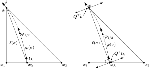
Figure 1: Two approaches to parametrizing a cubic curve approximating the characteristic $\boldsymbol{\varphi}$ leading from $\boldsymbol{x}_{\boldsymbol{\lambda}}$ to $\hat{\boldsymbol{x}}$ when numerically minimizing Fermat’s integral to compute $T(\hat{\boldsymbol{x}})$ and $\nabla T(\hat{\boldsymbol{x}})$. Left: $\boldsymbol{\varphi}$ is a cubic parametric curve with boundary data set directly from $\boldsymbol{x}_{\boldsymbol{\lambda}},\hat{\boldsymbol{x}},\boldsymbol{t}_{\boldsymbol{\lambda}}$, and $\hat{\boldsymbol{t}}$. Right: $\boldsymbol{\varphi}$ is the graph of a function in the orthogonal complement of $\operatorname{range}(\boldsymbol{\ell}^{\prime})$.

We consider two methods of choosing $\boldsymbol{\varphi}$ (see Figure 1). First, let $\boldsymbol{\ell}$ be interval connecting $\boldsymbol{x}_{\boldsymbol{\lambda}}$ to $\hat{\boldsymbol{x}}$, parametrized by arc length, and define:

(12) $$\boldsymbol{\ell}(\sigma)=\boldsymbol{x}_{\boldsymbol{\lambda}}+\sigma\boldsymbol{\ell}^{\prime},\qquad\boldsymbol{\ell}^{\prime}=(\hat{\boldsymbol{x}}-\boldsymbol{x}_{\boldsymbol{\lambda}})/L_{\boldsymbol{\lambda}}.$$

Using a cubic parametric curve

For one approach, we define:

(13) $$\boldsymbol{\varphi}(\sigma)=\boldsymbol{\ell}(\sigma)+\delta\boldsymbol{\varphi}(\sigma),$$

where $\delta\boldsymbol{\varphi}:[0,L]\to\Omega$ is a perturbation away from $\boldsymbol{\ell}$ that satisfies:

(14) $$\delta\boldsymbol{\varphi}(0)=0,\quad\delta\boldsymbol{\varphi}(L)=0,\quad\delta\boldsymbol{\varphi}^{\prime}(0)=\boldsymbol{t}_{\boldsymbol{\lambda}}-\boldsymbol{\ell}^{\prime},\quad\delta\boldsymbol{\varphi}^{\prime}(L)=\hat{\boldsymbol{t}}-\boldsymbol{\ell}^{\prime}.$$

We can explicitly write $\delta\boldsymbol{\varphi}$ as:

(15) $$\delta\boldsymbol{\varphi}(\sigma)=\big{(}\boldsymbol{t}_{\boldsymbol{\lambda}}-\boldsymbol{\ell}^{\prime}\big{)}K_{0}(\sigma)+\big{(}\hat{\boldsymbol{t}}-\boldsymbol{\ell}^{\prime}\big{)}K_{1}(\sigma),$$

where $K_{0},K_{1}:[0,L]\to\mathbb{R}$ are Hermite basis functions such that:

(16) $$\begin{split}K_{0}(0)=0=K_{0}(L),\qquad&K_{1}(0)=0=K_{1}(L),\\ K_{0}^{\prime}(0)=1=K_{1}^{\prime}(L),\qquad&K_{1}^{\prime}(0)=0=K_{0}^{\prime}(L).\end{split}$$

Explicitly, these are given by:

(17) $$K_{0}(\sigma)=\sigma-2\frac{\sigma^{2}}{L}+\frac{\sigma^{3}}{L^{2}},\qquad K_{1}(\sigma)=\frac{-\sigma^{2}}{L}+\frac{\sigma^{3}}{L^{2}}.$$

Let $\boldsymbol{t}_{\boldsymbol{\lambda}},\hat{\boldsymbol{t}}\in\mathbb{S}^{n-1}$ so that $\|\boldsymbol{t}_{\boldsymbol{\lambda}}\|=1=\|\hat{\boldsymbol{t}}\|$. As $L\to 0$, this results in a curve that is approximately parametrized by arc length: i.e., $\|\boldsymbol{\varphi}^{\prime}(\sigma)\|\to 1$ for all $\sigma$ such that $0\leq\sigma\leq L$ [16]. This simplifies the general cost function given by (9) to:

(18) $$F(\boldsymbol{\varphi})=\mathsf{T}(\boldsymbol{x}_{\boldsymbol{\lambda}})+\frac{L}{6}\Big{[}s(\boldsymbol{x}_{\boldsymbol{\lambda}})+4s\big{(}\boldsymbol{\varphi}_{1/2}\big{)}\big{\|}\boldsymbol{\varphi}^{\prime}_{1/2}\big{\|}+s(\hat{\boldsymbol{x}})\Big{]}.$$

Using (17), $\boldsymbol{\varphi}_{1/2}$ and $\boldsymbol{\varphi}^{\prime}_{1/2}$ can be written:

(19) $$\boldsymbol{\varphi}_{1/2}=\frac{\boldsymbol{x}_{\boldsymbol{\lambda}}+\hat{\boldsymbol{x}}}{2}+\frac{L}{8}\big{(}\boldsymbol{t}_{\boldsymbol{\lambda}}-\hat{\boldsymbol{t}}\big{)},\qquad\boldsymbol{\varphi}^{\prime}_{1/2}=\frac{3}{2}\boldsymbol{\ell}^{\prime}-\frac{\boldsymbol{t}_{\boldsymbol{\lambda}}+\hat{\boldsymbol{t}}}{4}.$$

Note that $\boldsymbol{\varphi}{}_{1/2}\sim(\boldsymbol{x}_{\boldsymbol{\lambda}}+\hat{\boldsymbol{x}})/2$ and $\boldsymbol{\varphi}^{\prime}{}_{1/2}\sim\boldsymbol{\ell}^{\prime}$ as $L\to 0$ if we assume that the wavefront is well-approximated by a plane wave near the update, since in this case $\boldsymbol{t}_{\boldsymbol{\lambda}}\sim\hat{\boldsymbol{t}}\sim\boldsymbol{\ell}^{\prime}$.

Parametrizing $\boldsymbol{\varphi}$ as the graph of a function

We can also define the perturbation away from $\boldsymbol{\ell}$ as the graph of a function; i.e., we assume that the perturbation is orthogonal to $\boldsymbol{\ell}^{\prime}$. Letting $\boldsymbol{Q}\in\mathbb{R}^{n\times(n-1)}$ be an orthogonal matrix such that $\boldsymbol{Q}^{\top}\boldsymbol{\ell}^{\prime}=0$, and letting $\boldsymbol{\zeta}:[0,L]\to\mathbb{R}^{n-1}$ be a curve specifying the components of the perturbation in this basis, we choose $\delta\boldsymbol{\varphi}(\sigma)=\boldsymbol{Q}\boldsymbol{\zeta}(\sigma)$ so that:

(20) $$\boldsymbol{\varphi}(\sigma)=\boldsymbol{\ell}(\sigma)+\boldsymbol{Q}\boldsymbol{\zeta}(\sigma).$$

where $\boldsymbol{\zeta}(\sigma)=\boldsymbol{b}_{0}K_{0}(\sigma)+\boldsymbol{b}_{1}K_{1}(\sigma)$. In this approach, instead of $\hat{\boldsymbol{t}}$ and $\boldsymbol{t}_{\boldsymbol{\lambda}}$, we optimize over $\boldsymbol{b}_{0},\boldsymbol{b}_{1}\in\mathbb{R}^{n-1}$. Now, noting that:

(21) $$\|\boldsymbol{\varphi}^{\prime}(\sigma)\|=\sqrt{\|\boldsymbol{\ell}^{\prime}\|^{2}+\|\boldsymbol{Q}\boldsymbol{\zeta}^{\prime}(\sigma)\|^{2}}=\sqrt{1+\|\boldsymbol{\zeta}^{\prime}(\sigma)\|^{2}},$$

we can write the cost functional $F$ as:

(22) $$\begin{split}F(\boldsymbol{\varphi})&=\mathsf{T}(\boldsymbol{x}_{\boldsymbol{\lambda}})+\frac{L}{6}\Bigg{[}s(\boldsymbol{x}_{\boldsymbol{\lambda}})\sqrt{1+\|\boldsymbol{b}_{0}\|^{2}}\\ &\hskip 30.00005pt+4s(\boldsymbol{\varphi}_{1/2})\sqrt{1+\|{(\boldsymbol{b}_{0}+\boldsymbol{b}_{1})}/4\|^{2}}+s(\hat{\boldsymbol{x}})\sqrt{1+\|\boldsymbol{b}_{1}\|^{2}}\Bigg{]}.\end{split}$$

Trade-offs between the two parametrizations of $\boldsymbol{\varphi}$

When $\boldsymbol{\varphi}$ is a cubic parametric curve, we run into an interesting problem described in more detail by Floater [16]. In particular, the order of accuracy of $\boldsymbol{\varphi}$ in approximating $\boldsymbol{\psi}$ is limited by our parametrization of $\boldsymbol{\varphi}$. If we parametrize $\boldsymbol{\varphi}$ over $\sigma\in[0,1]$ (that is uniformly), then the interpolant is at most $O(h^{2})$ accurate. If we parametrize it using a chordal parametrization, i.e. $\sigma\in[0,L]$, then it is at most $O(h^{4})$ accurate. Indeed, any Hermite spline using a chordal parametrization over each of its segment is at most $O(h^{4})$ accurate globally. To design a higher order solver than this requires us to parametrize $\boldsymbol{\varphi}$ using a more accurate approximation of the arc length of $\boldsymbol{\psi}$ (consider, e.g., using a quintic parametric curve). On the other hand, if we parametrize $\boldsymbol{\varphi}$ as the graph of a function, we can directly apply Hermite interpolation theory [45], and there is no such obstacle.

4 Different types of minimization problems

In this section, we consider four different ways of using $F$ to pose a minimization problem which would allow us to compute $T(\hat{\boldsymbol{x}})$. We note that each of these formulations is compatible with the version of $F$ where we take $\boldsymbol{\varphi}$ to be a parametric curve and where we define it as the graph of a function orthogonal to $\boldsymbol{\ell}(\sigma)$. Altogether, this leads to eight different JMMs.

4.1 Determining $\boldsymbol{t}_{\boldsymbol{\lambda}}$ by minimizing Fermat’s integral

Since the optimal $\boldsymbol{\varphi}$ is a characteristic of the eikonal equation, one approach to setting $\boldsymbol{t}_{\boldsymbol{\lambda}}$ and $\hat{\boldsymbol{t}}$ is to simply let them enter into the cost function as free parameters to be optimized over. This leads to the optimization problem:

(23) $$\begin{split}\mbox{minimize}&\quad F(\boldsymbol{x}_{\boldsymbol{\lambda}},\boldsymbol{t}_{\boldsymbol{\lambda}},\hat{\boldsymbol{t}})\\ \mbox{subject to}&\quad\boldsymbol{x}_{\boldsymbol{\lambda}}\in\operatorname{conv}(\boldsymbol{x}_{1},\ldots,\boldsymbol{x}_{n}),\\ &\quad\boldsymbol{t}_{\boldsymbol{\lambda}},\hat{\boldsymbol{t}}\in\mathbb{S}^{n-1},\end{split}$$

if we parametrize $\boldsymbol{\varphi}$ as a curve; or, if we parametrize $\boldsymbol{\varphi}$ as the graph of a function:

(24) $$\begin{split}\mbox{minimize}&\quad F(\boldsymbol{x}_{\boldsymbol{\lambda}},\boldsymbol{b}_{0},\boldsymbol{b}_{1})\\ \mbox{subject to}&\quad\boldsymbol{x}_{\boldsymbol{\lambda}}\in\operatorname{conv}(\boldsymbol{x}_{1},\ldots,\boldsymbol{x}_{n}),\\ &\quad\boldsymbol{b}_{0},\boldsymbol{b}_{1}\in\mathbb{R}^{n-1},\end{split}$$

For a $d$-dimensional update, the domain of each of these minimization problems has dimension $(d-1)(n-1)^{2}$, since $\dim(\operatorname{conv}(\boldsymbol{x}_{1},\ldots,\boldsymbol{x}_{d}))=d-1$.

4.2 Determining $\boldsymbol{t}_{\boldsymbol{\lambda}}$ from the eikonal equation

When we compute updates, we only require high-order accurate jets over $\operatorname{conv}(\boldsymbol{x}_{1},\ldots,\boldsymbol{x}_{n})$. This is a subset of $\Omega$ of codimension one: an interval in 2D, or triangle in 3D. If we know $T$ and $\nabla T$ at the vertices of this set, then we can use Hermite interpolation to compute $\mathsf{T}$. Unfortunately, this means that we can only approximate directional derivatives of $T$ in the linear span of this set. To compute $\nabla\mathsf{T}$, we need to recover the directional derivative normal to the facet.

Let $\tilde{\boldsymbol{V}}\in\mathbb{R}^{n\times(n-1)}$ be an orthogonal matrix such that:

(25) $$\operatorname{range}(\tilde{\boldsymbol{V}})=\operatorname{range}\left(\begin{bmatrix}\boldsymbol{x}_{2}-\boldsymbol{x}_{1}&\cdots&\boldsymbol{x}_{n}-\boldsymbol{x}_{1}\end{bmatrix}\right),$$

and let $\boldsymbol{v}\in\mathbb{R}^{n}$ be a unit vector such that $\tilde{\boldsymbol{V}}{}^{\top}\boldsymbol{v}=0$. Let $\nabla_{\tilde{\boldsymbol{V}}}$ be the gradient restricted to the range of $\tilde{\boldsymbol{V}}$, and likewise let $d_{\boldsymbol{v}}$ denote the $\boldsymbol{v}$-directional derivative. Then, from the eikonal equation, we have:

(26) $$s(\boldsymbol{x})^{2}=\|\nabla\tau(\boldsymbol{x})\|^{2}=|d_{\boldsymbol{v}}\tau(\boldsymbol{x})|^{2}+\|\nabla_{\tilde{\boldsymbol{V}}}\tau(\boldsymbol{x})\|^{2}.$$

To recover $\nabla\tau(\boldsymbol{x})$, first note that $\nabla\tau(\boldsymbol{x})$ should point in the same direction as $\boldsymbol{\ell}^{\prime}$. Choosing $\boldsymbol{v}$ so that $\boldsymbol{v}^{\top}\boldsymbol{\ell}^{\prime}>0$, we get:

(27) $$d_{\boldsymbol{v}}\tau(\boldsymbol{x})=\sqrt{s(\boldsymbol{x})^{2}-\|\nabla_{\tilde{\boldsymbol{V}}}\tau(\boldsymbol{x})\|^{2}}.$$

Letting $\boldsymbol{V}=\begin{bmatrix}\boldsymbol{v}&\tilde{\boldsymbol{V}}\end{bmatrix}$, equation (27) combined with $\nabla\tau(\boldsymbol{x})=\boldsymbol{V}\nabla_{\boldsymbol{V}}\tau(\boldsymbol{x})$ gives us a means of recovering $\nabla\tau(\boldsymbol{x})$ from $\nabla_{\tilde{\boldsymbol{V}}}\tau(\boldsymbol{x})$.

Using this technique, we can pose the following optimization problem:

(28) $$\begin{split}\mbox{minimize}&\quad F(\boldsymbol{x}_{\boldsymbol{\lambda}},\hat{\boldsymbol{t}})\\ \mbox{subject to}&\quad\boldsymbol{x}_{\boldsymbol{\lambda}}\in\operatorname{conv}(\boldsymbol{x}_{1},\ldots,\boldsymbol{x}_{n}),\\ &\quad\hat{\boldsymbol{t}}\in\mathbb{S}^{n-1},\end{split}$$

or, optimizing over $\boldsymbol{b}_{1}$ directly:

(29) $$\begin{split}\mbox{minimize}&\quad F(\boldsymbol{x}_{\boldsymbol{\lambda}},\boldsymbol{b}_{1})\\ \mbox{subject to}&\quad\boldsymbol{x}_{\boldsymbol{\lambda}}\in\operatorname{conv}(\boldsymbol{x}_{1},\ldots,\boldsymbol{x}_{n}),\\ &\quad\boldsymbol{b}_{1}\in\mathbb{R}^{n-1}\end{split}$$

For each $\boldsymbol{x}_{\boldsymbol{\lambda}}$, we set:

(30) $$\boldsymbol{t}_{\boldsymbol{\lambda}}\leftarrow\frac{\boldsymbol{V}\nabla_{\boldsymbol{V}}\mathsf{T}(\boldsymbol{x}_{\boldsymbol{\lambda}})}{\left\|\boldsymbol{V}\nabla_{\boldsymbol{V}}\mathsf{T}(\boldsymbol{x}_{\boldsymbol{\lambda}})\right\|}.$$

Note that the dimension of a $d$-dimensional update based on this minimization problem is $(d-1)(n-1)$

4.3 Determining $\boldsymbol{t}_{\boldsymbol{\lambda}}$ by marching cell-based interpolants

Another approach is to march cells that approximate the jet of the eikonal at each point. For example, if we have constructed a finite element interpolant using valid data on a cell whose boundary contains $\operatorname{conv}(\boldsymbol{x}_{1},\ldots,\boldsymbol{x}_{n})$ then we can evaluate its gradient to obtain:

(31) $$\boldsymbol{t}_{\boldsymbol{\lambda}}\leftarrow\frac{\nabla\mathsf{T}(\boldsymbol{x}_{\boldsymbol{\lambda}})}{\left\|\nabla\mathsf{T}(\boldsymbol{x}_{\boldsymbol{\lambda}})\right\|}.$$

We can combine this approach with the cost functional given by (28), albeit with a modified $\boldsymbol{t}_{\boldsymbol{\lambda}}$. We elaborate on how we march cells in section 7. An advantage of this approach is that it allows one to simultaneously march the second partials of $T$.

4.4 A simplified method using a quadratic curve

In some cases, in particular if the speed of sound is linear, i.e.:

(32) $$c(\boldsymbol{x})=\frac{1}{s(\boldsymbol{x})}=c_{0}+\boldsymbol{c}^{\top}\boldsymbol{x},\qquad c_{0}\in\mathbb{R},\qquad\boldsymbol{c}\in\mathbb{R}^{n},$$

the characteristic $\boldsymbol{\psi}$ is well-approximated by a quadratic. In this case, we again have a cost functional of the form (28).

If $\boldsymbol{\varphi}$ is parametrized as curve, we set $\boldsymbol{t}_{\boldsymbol{\lambda}}$ to be the reflection of $\hat{\boldsymbol{t}}$ across $\boldsymbol{\ell}^{\prime}$:

(33) $$\boldsymbol{t}_{\boldsymbol{\lambda}}=-\big{(}\boldsymbol{I}-2\hskip 1.00006pt\boldsymbol{\ell}^{\prime}\boldsymbol{\ell}^{\prime\top}\big{)}\hat{\boldsymbol{t}},$$

giving $\boldsymbol{t}_{\boldsymbol{\lambda}}+\hat{\boldsymbol{t}}=2\boldsymbol{\ell}^{\prime}\boldsymbol{\ell}^{\prime\top}\hat{\boldsymbol{t}}$ and $\boldsymbol{t}_{\boldsymbol{\lambda}}-\hat{\boldsymbol{t}}=-2\big{(}\boldsymbol{I}-\boldsymbol{\ell}^{\prime}\boldsymbol{\ell}^{\prime\top}\big{)}\hat{\boldsymbol{t}}$. Then:

(34) $$\boldsymbol{\varphi}_{1/2}=\frac{\boldsymbol{x}_{\boldsymbol{\lambda}}+\hat{\boldsymbol{x}}}{2}-\frac{L}{4}\big{(}\boldsymbol{I}-\boldsymbol{\ell}^{\prime}\boldsymbol{\ell}^{\prime\top}\big{)}\hat{\boldsymbol{t}},\qquad\boldsymbol{\varphi}^{\prime}_{1/2}=\frac{3+\boldsymbol{\ell}^{\prime\top}\hat{\boldsymbol{t}}}{2}\boldsymbol{\ell}^{\prime}.$$

This simplifies $F$ given by (18) to:

(35) $$F(\boldsymbol{x}_{\boldsymbol{\lambda}},\hat{\boldsymbol{t}})=\mathsf{T}(\boldsymbol{x}_{\boldsymbol{\lambda}})+\frac{L}{6}\bigg{[}s(\boldsymbol{x}_{\boldsymbol{\lambda}})+2\big{(}3+\boldsymbol{\ell}^{\prime\top}\hat{\boldsymbol{t}}\big{)}s\Big{(}\frac{\boldsymbol{x}_{\boldsymbol{\lambda}}+\hat{\boldsymbol{x}}}{2}-\frac{L}{4}\big{(}\boldsymbol{I}-\boldsymbol{\ell}^{\prime}\boldsymbol{\ell}^{\prime\top}\big{)}\Big{)}+s(\hat{\boldsymbol{x}})\bigg{]}.$$

If $\boldsymbol{\varphi}$ is parametrized as the graph of a function, then:

(36) $$\boldsymbol{\zeta}_{1/2}=\frac{\hat{\boldsymbol{x}}+\boldsymbol{x}_{\boldsymbol{\lambda}}}{2}+\frac{L}{4}\boldsymbol{Q}^{\top}\hat{\boldsymbol{t}},\qquad\boldsymbol{\zeta}^{\prime}=0,$$

simplifying the version of $F$ in (22) to:

(37) $$F(\boldsymbol{x}_{\boldsymbol{\lambda}},\hat{\boldsymbol{t}})=\mathsf{T}(\boldsymbol{x}_{\boldsymbol{\lambda}})+\frac{L}{6}\bigg{[}\big{(}s(\boldsymbol{x}_{\boldsymbol{\lambda}})+s(\hat{\boldsymbol{x}})\big{)}\sqrt{1+\|\boldsymbol{b}_{0}\|^{2}}+4s(\boldsymbol{\varphi}_{1/2})\bigg{]}.$$

since $\boldsymbol{Q}^{\top}\hat{\boldsymbol{t}}=\boldsymbol{b}_{0}=-\boldsymbol{b}_{1}$.

4.5 Other approaches

We tried two other approaches which failed to provide satisfactory results:

• A combination of the quadratic simplification in subsection 4.4 with the methods in subsections 4.2 or 4.3. In this case, we use our knowledge of $\nabla T(\boldsymbol{x}_{\boldsymbol{\lambda}})$ along the base of the update to choose $\hat{\boldsymbol{t}}$ and $\boldsymbol{t}_{\boldsymbol{\lambda}}$. This reduces the dimensionality of the cost function to $d-1$. However, except for in special cases (e.g. $s\equiv 1$), this propagates errors in a manner that causes the solver to diverge; or, at best, allows it converge with $O(h)$ accuracy. We note that if $s\equiv 1$, still simpler methods can be used, so this combination of approaches does not seem to be useful.

• We can extract not only $\boldsymbol{t}_{\boldsymbol{\lambda}}$ from the Hermite interpolant on $\operatorname{conv}(\boldsymbol{x}_{1},\ldots,\boldsymbol{x}_{n})$, but also $\boldsymbol{\varphi}^{\prime\prime}(0)$. From the Euler-Lagrange equations for the eikonal equation, we obtain:

  (38) $$\boldsymbol{Q}^{\top}\nabla s(\boldsymbol{x}_{\boldsymbol{\lambda}})=s(\boldsymbol{x}_{\boldsymbol{\lambda}})\frac{\boldsymbol{Q}^{\top}\boldsymbol{\varphi}^{\prime\prime}(0)}{\|\boldsymbol{\varphi}^{\prime}(0)\|}.$$

  With $\boldsymbol{\varphi}$ parametrized as a graph, we have $\boldsymbol{Q}^{\top}\boldsymbol{\varphi}^{\prime\prime}(0)=\boldsymbol{\zeta}^{\prime\prime}(0)$, giving:

  (39) $$\boldsymbol{\zeta}^{\prime\prime}(0)=\frac{\boldsymbol{Q}^{\top}\nabla s(\boldsymbol{x}_{\boldsymbol{\lambda}}){(1+\|\boldsymbol{Q}^{\top}\boldsymbol{x}_{\boldsymbol{\lambda}}\|^{2})}}{s(\boldsymbol{x}_{\boldsymbol{\lambda}})}.$$

  This completely defines $\boldsymbol{\varphi}$ as the graph of a cubic polynomial using the graph parametrization. Unfortunately, this method diverges for the same reason as the method described in the previous bullet.

4.6 A warm start

Certain of the optimization problems in the preceding section are clearly nonconvex; e.g., (23) is nonconvex since its domain, the product of $\operatorname{conv}(\boldsymbol{x}_{1},\ldots,\boldsymbol{x}_{n})$ and two copies of $\mathbb{S}^{n-1}$, is nonconvex. For $h$ small, if $\boldsymbol{x}_{\boldsymbol{\lambda}}$ is nearly optimal, then the optimal local ray $\boldsymbol{\varphi}$ should be close to $\boldsymbol{\ell}$, the straight line segment connecting $\boldsymbol{x}_{\boldsymbol{\lambda}}$ and $\hat{\boldsymbol{x}}$. This suggests an approach to finding an initial iterate (a warm start) for (23) or the other optimization problems considered (i.e., (24), (28), and (29)). In 2D, following a similar approach to the simplified midpoint rule (denoted “mp0”) rule used in our earlier work on ordered line integral methods (OLIMs) for the solving the eikonal equation [30], we let $\mathsf{T}$ be a cubic Hermite polynomial approximation of $\tau$ over $\lambda\in[0,1]$ and approximate (5) by solving:

(40) $$\begin{split}\mbox{minimize}&\quad\mathsf{T}(\lambda)+\frac{L}{2}\Big{(}s(\boldsymbol{x}_{\lambda})+s(\hat{\boldsymbol{x}})\Big{)},\\ \mbox{subject to}&\quad 0\leq\lambda\leq 1.\end{split}$$

After solving this problem, we can compute an initial iterate for (23) from $\lambda^{*}$, the optimum of (40). For example, we set $\boldsymbol{x}_{\lambda}\leftarrow\boldsymbol{x}_{\lambda^{*}}$; we set $\boldsymbol{t}_{\lambda}$ using $\lambda^{*}$ and one of the approaches outlined in the preceding sections; and, if required, we set $\hat{\boldsymbol{t}}\leftarrow(\hat{\boldsymbol{x}}-\boldsymbol{x}_{\lambda^{*}})/\|\hat{\boldsymbol{x}}-\boldsymbol{x}_{\lambda^{*}}\|$. In practice, (40) can be solved rapidly and robustly using a rootfinder.

4.7 Optimization algorithms

We do not dwell on the details of how to numerically solve the minimization problems in the preceding sections. We make some general observations:

• These optimization problems are very easy to solve—what’s costly is that we have to solve $O(N)$ of them. As $h\to 0$, they are strictly convex and well-behaved. Empirically, Newton’s method converges in $O(1)$ steps (typically fewer than 5 with a well-chosen warm start—see section 4.6). We leave a detailed comparison of different approaches to numerically solving these optimization problems for future work.

• The gradients and Hessians of these cost functions are somewhat complicated. Programming them can be tricky and tedious, suggesting that automatic differentiation may be a worthwhile approach [26, 19].

• The constraint $\boldsymbol{x}_{\boldsymbol{\lambda}}\in\operatorname{conv}(\boldsymbol{x}_{1},\ldots,\boldsymbol{x}_{n})$ corresponds to a set of linear inequality constraints, which are simple to incorporate. Because of the form of these constraints, checking the KKT conditions at the boundary is cheap and easy [30, 49]. See the next section on skipping updates.

• The constraints $\boldsymbol{t}_{\boldsymbol{\lambda}},\hat{\boldsymbol{t}}\in\mathbb{S}^{n-1}$ are nonlinear; however, they can be eliminated. If $n=2$, then we can set $\hat{\boldsymbol{t}}=(\cos(\theta),\sin(\theta))$, letting $\theta\in\mathbb{R}$. For $n>2$, we can use a Riemannian Newton’s method for minimization on $\mathbb{S}^{n-1}$, which is simple to implement and known to converge superlinearly [1]. Alternatively, we could use spherical coordinates, although the expressions become unwieldy.

5 Hierarchical update algorithms

Away from shocks, where multiple wavefronts collide, exactly one characteristic will pass through a point $\hat{\boldsymbol{x}}$. When we minimize $F$ over each update in the stencil, the characteristic will pass through the base of the minimizing update, or possibly through the boundary of several adjacent updates. We can use this fact to sequence the updates that are performed to design a work-efficient solver. In our previous work on ordered line integral methods (OLIMs), we explored variations of this idea [30, 49]. An approach that works well is the bottom-up update algorithm.

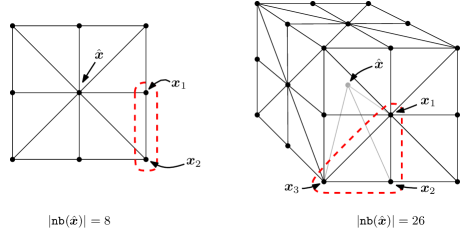
Figure 2: The neighborhoods typically used by semi-Lagrangian solvers in 2D and 3D on a regular grid. These are the stencils used by Tsitsiklis’s algorithm and two of the OLIM stencils [46, 30]. Left: “olim8” in $\mathbb{R}^{2}$. This is the 8-point stencil used in this paper. Right: “olim26” in $\mathbb{R}^{3}$.

To fix the idea in 3D, consider $\texttt{nb}(\boldsymbol{x})$ as shown in Figure 2, for which $|\texttt{nb}(\boldsymbol{x})|=26$. There are 26 “line” updates, where $d=1$. To start with, each valid line update is done, and $\boldsymbol{x}_{1}$ for the minimizing line update is recorded. Next, we fix $\boldsymbol{x}_{1}$ and perform “triangle” updates ($d=2$) where $\boldsymbol{x}_{2}$ is varying. In this case, we can restrict the number of triangle updates that are done by assuming either that $(\boldsymbol{x}_{1},\boldsymbol{x}_{2})$ is an edge of mesh discretizing the surface of the 3D stencil shown in Figure 2, or that $\|\boldsymbol{x}_{1}-\boldsymbol{x}_{2}\|$ is small enough (measuring the distance of these two points in different norms leads to a different number of triangle updates—we find the $\ell_{1}$ norm to work well). Finally, we fix $\boldsymbol{x}_{2}$ corresponding to the minimizing triangle update, and do tetrahedron updates containing $\boldsymbol{x}_{1}$ and $\boldsymbol{x}_{2}$. Throughout this process, $\boldsymbol{x}_{1},\boldsymbol{x}_{2}$, and $\boldsymbol{x}_{3}$ must all be valid.

We emphasize that our work-efficient OLIM update algorithms work equally well for the class of algorithms developed here. The main differences between the JMMs studied here and the earlier OLIMs are the cost functionals and the we way approximate $T$.

6 Initialization methods

A common problem with the convergence of numerical methods for solving the eikonal equation concerns how to treat rarefaction fans. Our numerical tests consist of point source problems, around which a rarefaction forms. A standard approach is to introduce the factored eikonal equation [17, 24, 31]. If a point source is located at $\boldsymbol{x}^{\circ}\in\Omega_{h}$ and if we set $\Gamma_{h}=\{\boldsymbol{x}^{\circ}\}$, then we let $d(\boldsymbol{x})=\|\boldsymbol{x}-\boldsymbol{x}^{\circ}\|$ and use the ansatz:

(41) $$\tau(\boldsymbol{x})=z(\boldsymbol{x})+d(\boldsymbol{x}),\qquad\boldsymbol{x}\in\Omega.$$

We insert this into the eikonal equation, modifying our numerical methods as necessary, and solve for $z(\boldsymbol{x})$ instead. This is not complicated—see our previous work on OLIMs for solving the eikonal equation to see how the cost functions should generally be modified [30, 49].

Yet another approach would be to solve the characteristic equations to high-order for each $\boldsymbol{x}$ in such a ball. This would require solving $O(N)$ boundary value problems, each discretized into $O(N^{1/3})$ intervals, resulting in an $O(N^{4/3})$ cost overall (albeit with a very small constant). One issue with this approach is that it only works well if the ball surrounding $\boldsymbol{x}^{\circ}$ is contained in the interior of $\Omega$. For our numerical experiments, we simply initialize $T$ and $\nabla T$ to the correct, ground truth values in a ball or box of constant size centered at $\boldsymbol{x}^{\circ}$.

7 Cell marching

Of particular interest is solving the transport equation governing the amplitude $\alpha$ while simultaneously solving the eikonal equation. Equation (4) can be solved using upwind finite differences [5] or paraxial raytracing [29]. We prefer the latter approach since it can be done locally, using the characteristic path $\boldsymbol{\varphi}$ recovered when computing $T(\hat{\boldsymbol{x}})$. Either approach requires accurate second derivative information (we need $\Delta T$ for upwind finite differences, or $\nabla^{2}T$ for paraxial raytracing).

For the purposes of explanation and our numerical tests, we consider a rectilinear grid with square cells in $\mathbb{R}^{2}$. On each cell, our goal is to build a bicubic interpolant, approximating $T(\boldsymbol{x})$. This requires knowing $T,\nabla T$, and $T_{xy}$ at each cell corner. If we know these values with $O(h^{4-p})$ accuracy, where $p$ is the order of the derivative, then the bicubic is $O(h^{4-p})$ accurate over the cell. So far, we have described an algorithm that marches $T$ and $\nabla T$, which together constitute the total 1-jet. We now show how $T_{xy}$ can also be marched, allowing us to march the partial 1-jet.

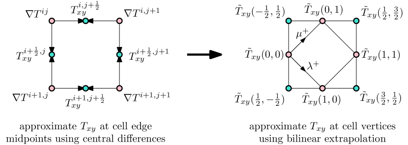
Figure 3: Cell-based interpolation. To approximate the mixed second partials of a function with $O(h^{2})$ accuracy from $O(h^{3})$ accurate gradient values available at the corners of a cell, the following method of using central differences to approximate the mixed partials at the midpoints of the edges of the cell, followed by bilinear extrapolation, can be used.

Let $\boldsymbol{x}_{ij}$ with $(i,j)\in\{0,1\}^{2}$ denote the corners of a square cell with sides of length $h$, and assume that we know $\nabla T(\boldsymbol{x}_{ij})$ with $O(h^{3})$ accuracy. We can use the following approach to estimate $T_{xy}(\boldsymbol{x}_{ij})$ at each corner:

• First, at the midpoints of the edges oriented in the $x$ direction (resp., $y$ direction), approximate $T_{xy}$ using the central differences involving $T_{y}$ (resp., $T_{x}$) at the endpoints. This approximation is $O(h^{2})$ accurate at the midpoints.

• Use bilinear extrapolation to reevaluate $T_{xy}$ at the corners of the cell, yielding $T_{xy}(\boldsymbol{x}_{ij})$, also with $O(h^{2})$ accuracy.

This procedure is illustrated in Figure 3.

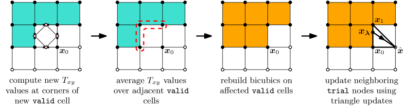
Figure 4: Local cell marching. After computing values of $T_{xy}$ as shown in Figure 3 (left), to ensure continuity of the global interpolant, nodal values incident on the newly valid cell (containing $x_{0}$) can be recomputed by averaging over $T_{xy}$ values taken from incident valid cells (middle). Finally, a bicubic cell-based interpolant is constructed (right).

One issue with this approach is that it results in a piecewise interpolant that is only $C^{1}$ globally. That is, if we estimate the value of $T_{xy}$ at a corner from each of the cells which are incident upon it, we will get different values in general. To compute a globally $C^{2}$ piecewise interpolant, we can average $T_{xy}$ values over incident valid cells, where we define a valid cell to be a cell whose vertices are all valid. How to do this is shown in Figure 4.

The idea of approximating the partial 1-jet from the total 1-jet in an optimally local fashion by combining central differences with bilinear extrapolation, and averaging nodal values over adjacent cells to increase the degree of continuity of the interpolant, is borrowed from Seibold et al. [37]. However, applying this idea in this context, and doing the averaging in an upwind fashion is novel.

The scheme arrived at in this way is no longer optimally local. However, the sequence of operations described here can be done on an unstructured triangle or tetrahedron mesh. This makes this approach suitable for use with an unstructured mesh that conforms to a complicated boundary. We should mention here that our approach to estimating $T_{xy}$ is referred to as twist estimation in the computer-aided design (CAD) community [15], where other approaches have been proposed [10, 20]. We leave adapting these ideas to the present context for future work.

7.1 Marching the amplitude

In this section we show how to compute a numerical approximation of $\alpha$, denoted $A:\Omega_{h}\to\mathbb{R}$. One simple approach would be to discretize (4) using upwind finite differences and compute $A(\hat{\boldsymbol{x}})$ using valid nodes after $T(\hat{\boldsymbol{x}})$ and $\nabla T(\hat{\boldsymbol{x}})$. One potential shortcoming of this approach is that $A$ is singular at caustics. Instead, we will explore using paraxial raytracing to compute $A$ in this section [28]. The background material on paraxial raytracing used in this section can be found in more detail in M. Popov’s book [29].

The basic idea of paraxial raytracing is to consider a fixed, central ray, which we denote $\boldsymbol{\varphi}_{0}$, and a surrounding tube of rays, parametrized by:

(42) $$\boldsymbol{\varphi}(\sigma,\boldsymbol{q})=\boldsymbol{\varphi}_{0}(\sigma)+\boldsymbol{E}(\sigma)\boldsymbol{q},$$

where $\boldsymbol{E}:[0,L]\to\mathbb{R}^{n\times(n-1)}$ is an orthogonal matrix such that $\boldsymbol{E}^{\top}\boldsymbol{\varphi}_{0}^{\prime}\equiv 0$. For each $\boldsymbol{q}$, the corresponding ray should satisfy the Euler-Lagrange equations for (1). If we let $c_{0}(\sigma)=c(\boldsymbol{\varphi}_{0}(\sigma))$, where $c=1/s$, then $\boldsymbol{q}$ along with the conjugate momenta $\boldsymbol{p}$ (the exact form of which is not important in this instance) will satisfy:

(43) $$\begin{bmatrix}d\boldsymbol{q}/d\sigma\\ d\boldsymbol{p}/d\sigma\end{bmatrix}=\begin{bmatrix}&c_{0}(\sigma)\boldsymbol{I}\\ \frac{-1}{c_{0}(\sigma)^{2}}\left.\frac{\partial^{2}c}{\partial\boldsymbol{q}\partial\boldsymbol{q}^{\top}}\right|_{\boldsymbol{q}=0}&\end{bmatrix}\begin{bmatrix}\boldsymbol{q}\\ \boldsymbol{p}\end{bmatrix}.$$

If we let $\boldsymbol{Q}(\sigma),\boldsymbol{P}(\sigma):[0,L]\to\mathbb{R}^{(n-1)\times(n-1)}$ be a linearly independent set of solutions to (43), then along the central ray, the amplitude satisfies:

(44) $$A(\boldsymbol{\varphi}_{0}(\sigma))=\sqrt{\frac{c_{0}(\sigma)}{|\det(\boldsymbol{Q}(\sigma))|}}A(\boldsymbol{\varphi}_{0}(0)).$$

Note that when we compute an update, we obtain a cubic path $\boldsymbol{\varphi}$ approximating a ray of (1), such that $\boldsymbol{\varphi}(0)=\boldsymbol{x}_{\boldsymbol{\lambda}}$ and $\boldsymbol{\varphi}(L)=\hat{\boldsymbol{x}}$.

The quantity $|\det(\boldsymbol{Q}(\sigma))|$ is known as the geometric spreading along the ray tube. We denote it $J(\sigma)$. Letting $\mathsf{A}$ denote a polynomial approximation of $A$ off of the grid nodes in $\Omega_{h}$, using Eq. 44, we can compute $A(\hat{\boldsymbol{x}})$ from:

(45) $$A(\hat{\boldsymbol{x}})=\sqrt{\frac{c_{0}(L_{\boldsymbol{\lambda}})}{|\det(\boldsymbol{Q}(L_{\boldsymbol{\lambda}}))|}}\mathsf{A}(\boldsymbol{x}_{\boldsymbol{\lambda}})=\sqrt{\frac{c(\hat{\boldsymbol{x}})}{J(\boldsymbol{x}_{\boldsymbol{\lambda}})}}\mathsf{A}(\boldsymbol{x}_{\boldsymbol{\lambda}}).$$

Since this depends on $\boldsymbol{Q}(L)$, we must solve (43) along $\boldsymbol{\varphi}$, requiring us to provide initial conditions at $\sigma=0$. Note that if we set $\sigma=0$ in (44), we can see that $|\det(\boldsymbol{Q}(0))|=c_{0}(0)$ is necessary. A simple choice for the initial conditions for $\boldsymbol{Q}$ is $\boldsymbol{Q}(0)=c_{0}(0)^{1/n}\boldsymbol{I}$. This assumes that we aren’t too close to a point source, where $A$ is singular.

To find initial conditions for $\boldsymbol{P}$, first expand $\tau$ in a Taylor series orthogonal to the central ray, i.e. in the coordinates $\boldsymbol{q}$. Doing this, we find that:

(46) $$\tau(\varphi(\sigma,\boldsymbol{q}))=\tau(\varphi_{0}(\sigma))+\frac{1}{2}\boldsymbol{q}^{\top}\left.\frac{\partial^{2}\tau}{\partial\boldsymbol{q}\partial\boldsymbol{q}^{\top}}\right|_{\boldsymbol{q}=0}\boldsymbol{q}+O(\boldsymbol{q}^{3}).$$

In this Taylor expansion, the linear term disappears since the rays and wavefronts are orthogonal. If we let:

(47) $$\boldsymbol{\Gamma}=\left.\frac{\partial^{2}\tau}{\partial\boldsymbol{q}\partial\boldsymbol{q}^{\top}}\right|_{\boldsymbol{q}=0},$$

we find that $\boldsymbol{\Gamma}$ satisfies the matrix Ricatti equation:

(48) $$\frac{d\boldsymbol{\Gamma}}{d\sigma}+c_{0}\boldsymbol{\Gamma}^{2}+\frac{1}{c_{0}^{2}}\left.\frac{\partial^{2}c}{\partial\boldsymbol{q}\partial\boldsymbol{q}^{\top}}\right|_{\boldsymbol{q}=0}=0.$$

The standard way to solve (48) is to use the ansatz $\boldsymbol{\Gamma}=\boldsymbol{P}\boldsymbol{Q}^{-1}$, which, indeed, leads us back to (43). However, this viewpoint furnishes us with the initial conditions for $\boldsymbol{P}$, since $\boldsymbol{\Gamma}(0)$ can now be readily computed from $\nabla^{2}\mathsf{T}(\boldsymbol{x}_{\boldsymbol{\lambda}})$.

Marching the amplitude of a linear speed of sound

As a simple but important test case, we consider a problem with a constant speed of sound, i.e.:

(49) $$s(\boldsymbol{x})=\frac{1}{c(\boldsymbol{x})},\qquad c(\boldsymbol{x})=v_{0}+\boldsymbol{v}^{\top}\boldsymbol{x}.$$

In this case, (43) simplifies considerably since $\nabla^{2}c\equiv 0$, implying $\boldsymbol{P}(\sigma)\equiv\boldsymbol{P}(0)=\boldsymbol{\Gamma}(0)\boldsymbol{Q}(0)$. From this, we can integrate $d\boldsymbol{Q}/d\sigma$ from 0 to $L$ to obtain:

(50) $$\boldsymbol{Q}(L)=\Bigg{[}\boldsymbol{I}+\bigg{(}\int_{0}^{L}c(\boldsymbol{\varphi}(\sigma))d\sigma\bigg{)}\boldsymbol{\Gamma}(0)\Bigg{]}\boldsymbol{Q}(0).$$

Denote the integral in this expression for $\boldsymbol{Q}(L)$ by $\epsilon$. To evaluate $\epsilon$ approximately, we can apply the trapezoid rule to get:

(51) $$\epsilon=\int_{0}^{L}c(\boldsymbol{\varphi}(\sigma))d\sigma=L\cdot\left(v_{0}+\boldsymbol{v}^{\top}(\hat{\boldsymbol{x}}+\boldsymbol{x}_{\boldsymbol{\lambda}})/2\right)+O(L^{2}),$$

which implies that $|\epsilon|=O(L)$. The fact that the error is $O(L^{2})$ in this case follows from usual error bound for the trapezoid rule and the fact that $\max_{0\leq\sigma\leq L}|\boldsymbol{\varphi}^{\prime\prime}(\sigma)|=O(L^{-1})$, by our choice of parametrization.

We would like to develop a simple update rule for the geometric spreading. First, note that the determinant satisfies the following identity:

(52) $$\det(\boldsymbol{I}+\epsilon\boldsymbol{\Gamma}(0))=1+\epsilon\operatorname{tr}(\boldsymbol{\Gamma}(0))+O(\epsilon^{2}).$$

Next, recall that $\boldsymbol{E}(0)$ is an orthogonal matrix such that $\boldsymbol{E}(0)^{\top}\boldsymbol{\varphi}_{0}^{\prime}=\boldsymbol{E}(0)^{\top}\boldsymbol{t}_{\boldsymbol{\lambda}}=0$. Let $\boldsymbol{U}=\begin{bmatrix}\boldsymbol{E}(0)&\boldsymbol{t}_{\boldsymbol{\lambda}}\end{bmatrix}$ and write:

(53) $$\operatorname{tr}\nabla^{2}T(\boldsymbol{x}_{\boldsymbol{\lambda}})=\operatorname{tr}\boldsymbol{U}^{\top}\nabla^{2}T(\boldsymbol{x}_{\boldsymbol{\lambda}})\boldsymbol{U}=\operatorname{tr}\boldsymbol{E}(0)^{\top}\nabla^{2}T(\boldsymbol{x}_{\boldsymbol{\lambda}})\boldsymbol{E}(0)+\boldsymbol{t}_{\boldsymbol{\lambda}}^{\top}\nabla^{2}T(\boldsymbol{x}_{\boldsymbol{\lambda}})\boldsymbol{t}_{\boldsymbol{\lambda}}.$$

By definition, $\boldsymbol{\Gamma}(0)=\boldsymbol{E}(0)^{\top}\nabla^{2}T(\boldsymbol{x}_{\boldsymbol{\lambda}})\boldsymbol{E}(0)$. Taking the gradient of (1), we get:

(54) $$\nabla^{2}T(\boldsymbol{x}_{\boldsymbol{\lambda}})\nabla T(\boldsymbol{x}_{\boldsymbol{\lambda}})=s(\boldsymbol{x}_{\boldsymbol{\lambda}})\nabla s(\boldsymbol{x}_{\boldsymbol{\lambda}}),$$

which leads immediately to:

(55) $$\boldsymbol{t}_{\boldsymbol{\lambda}}^{\top}\nabla^{2}T(\boldsymbol{x}_{\boldsymbol{\lambda}})\boldsymbol{t}_{\boldsymbol{\lambda}}=\boldsymbol{t}_{\boldsymbol{\lambda}}^{\top}\nabla s(\boldsymbol{x}_{\boldsymbol{\lambda}}),$$

noting that $\boldsymbol{t}_{\boldsymbol{\lambda}}=\nabla T(\boldsymbol{x}_{\boldsymbol{\lambda}})/\|\nabla T(\boldsymbol{x}_{\boldsymbol{\lambda}})\|$. Combining (53) and (55) gives:

(56) $$\operatorname{tr}\boldsymbol{\Gamma}(0)=\Delta T(\boldsymbol{x}_{\boldsymbol{\lambda}})-\boldsymbol{t}_{\boldsymbol{\lambda}}^{\top}\nabla s(\boldsymbol{x}_{\boldsymbol{\lambda}}),$$

since $\operatorname{tr}\nabla^{2}T(\boldsymbol{x}_{\boldsymbol{\lambda}})=\Delta T(\boldsymbol{x}_{\boldsymbol{\lambda}})$. This gives the following update for $J$:

(57) $$J(\hat{\boldsymbol{x}})=\Big{|}1+\epsilon\cdot\big{(}\Delta T(\boldsymbol{x}_{\boldsymbol{\lambda}})-\boldsymbol{t}_{\boldsymbol{\lambda}}^{\top}\nabla s(\boldsymbol{x}_{\boldsymbol{\lambda}})\big{)}\Big{|}\cdot\mathsf{J}(\boldsymbol{x}_{\boldsymbol{\lambda}}).$$

Here, $\mathsf{J}$ denotes a local polynomial approximation to $J$. This can be computed directly from data immediately available after solving the optimization problem that determines $T(\hat{\boldsymbol{x}})$ and $\nabla T(\hat{\boldsymbol{x}})$.

Initial data for $J$ and $A$

Determing the initial data for the amplitude is involved [3, 4, 29, 32], and detailed consideration of this problem is outside the scope of this work. Instead, we note that for a point source in 2D, the following hold approximately near the point source:

(58) $$J(\boldsymbol{x})\sim|\boldsymbol{x}|,\qquad A(\boldsymbol{x})\sim\frac{e^{i\pi/4}}{2\sqrt{2\pi\omega}}\sqrt{\frac{c(\boldsymbol{x})}{J(\boldsymbol{x})}}.$$

See Popov for quick derivations of these approximations [29]. In our test problems, we initialize $J$ to $|\boldsymbol{x}|$ near the point source, march $J$ according to (57) where $\mathsf{J}=(1-\lambda)J(\boldsymbol{x}_{1})+\lambda J(\boldsymbol{x}_{2})$, and compute the final amplitude from:

(59) $$A(\boldsymbol{x})=\frac{e^{i\pi/4}}{2\sqrt{2\pi\omega}}\sqrt{\frac{c(\boldsymbol{x})}{J(\boldsymbol{x})}}.$$

We emphasize that this is only valid for two-dimensional problems. The same sort of approach can be used for 3D problems, but (58) must be modified.

Marching the amplitude for more general slowness functions

The update given by (57) is valid if we approximate the speed function $c=1/s$ with a piecewise linear function with nodal values taken from $c(\boldsymbol{x})$, where $\boldsymbol{x}\in\Omega_{h}$. This should be a reasonable thing to do, since the update rule given by (57) in this case appears to be $O(h^{2})$ accurate. Since the accuracy of $\nabla^{2}T$ computed by our method is limited, we should not expect to be able to obtain much better than $O(h)$ accuracy for $J$. That said, a more accurate update for $J$ could be obtained by numerically integrating (43).

8 Numerical experiments

In this section, we first present a variety of test problems which differ primarily in the choice of slowness function $s$. The choices of $s$ range from simple, such as $s\equiv 1$ (an overly simplified but reasonable choice for speed of sound in room acoustics), to more strongly varying. We then present experimental results for our different JMMs as applied to these different slowness functions, demonstrating the significant effect the choice of $s$ has on solver accuracy. The solvers used in these experiments are:

• JMM1: $\boldsymbol{\varphi}$ is approximated using a cubic curve, and tangent vectors are found by solving 23.

• JMM2: $\boldsymbol{\varphi}$ is approximated using a cubic curve, with $\hat{\boldsymbol{t}}$ optimized from 28 and $\boldsymbol{t}_{\boldsymbol{\lambda}}$ found from Hermite interpolation at the base of the update.

• JMM3: $\boldsymbol{\varphi}$ is approximated using a quadratic curve, with its tangent vectors being found by optimizing.

• JMM4: JMM2 combined with the cell-marching method described in section 7.

We also plot the same results obtained by the FMM [38] and olim8_mp0 [30]. We do not include least squares fits for these solvers in our tables. They are mostly $O(h)$, with some exceptions for $\nabla T$ as computed by the FMM.

We note that $s$ does not significantly affect the runtime of any of our solvers—formally, our solvers run in $O(|\Omega_{h}|\log|\Omega_{h}|)$ time, where the constant factors are essentially insensitive to the choice of $s$. We note that the cost of updating the heap is very small compared to the cost of doing updates. Since only $|\Omega_{h}|$ updates must be computed, the CPU time of the solver effectively scales like $O(|\Omega_{h}|)$ for all problem sizes considered in this paper.

8.1 Test problems

In this section, we provide details for the test problems used in our numerical tests.

Constant slowness with a point source

For this problem, the slowness and solution are given by:

(60) $$s\equiv 1,\qquad\tau(\boldsymbol{x})=\|\boldsymbol{x}\|.$$

We take the domain to be $\Omega=[-1,1]\times[-1,1]\subseteq\mathbb{R}^{2}$. To control the size of the discretized domain, we let $M>0$ be an integer and set $h=1/M$, from which we define $\Omega_{h}$ accordingly. We place a point source at $\boldsymbol{x}^{\circ}=(0,0)\in\Omega_{h}$. The set of initial boundary data locations given by is $\Gamma_{h}=\{\boldsymbol{x}^{\circ}\}$, with boundary conditions given by $g(\boldsymbol{x}^{\circ})=0$.

Linear speed with a point source (#1)

Our next test problem has a linear velocity profile. This might model the variation in the speed of sound due to a linear temperature gradient (e.g., in a large room). The slowness is given by [17, 44]:

(61) $$s(\boldsymbol{x})=\left[\frac{1}{s_{0}}+\boldsymbol{v}^{\top}\boldsymbol{x}\right]^{-1},$$

where $s_{0}>0$, and $\boldsymbol{v}\in\mathbb{R}^{2}$ are parameters. The solution is given by:

(62) $$\tau(\boldsymbol{x})=\frac{1}{\|\boldsymbol{v}\|}\cosh^{-1}\left(1+\frac{1}{2}s_{0}s(\boldsymbol{x})\|\boldsymbol{v}\|^{2}\|\boldsymbol{x}\|^{2}\right).$$

For our first test with a linear speed function, we take $s_{0}=1$ and $\boldsymbol{v}=(0.133,-0.0933)$. For this problem, $\Omega=[-1,1]\times[-1,1]$, $\Gamma_{h}=\{\boldsymbol{x}^{\circ}\}$, and $g(\boldsymbol{x}^{\circ})=0$.

Linear speed with a point source (#2)

For our second linear speed test problem, we set $s_{0}=2$ and $\boldsymbol{v}=(0.5,0)$ as in [31]. For this problem, we let $\Omega=[0,1]\times[0,1]$, discretize into $M$ nodes along each axis, and define $\Omega_{h}$ accordingly (i.e., $|\Omega_{h}|=M^{2}$, with $M=h^{-1}$). We take $\boldsymbol{x}^{\circ}$, $\Gamma_{h}$, and $g$ to be same as in the previous two test problems.

A nonlinear slowness function involving a sine function

For $\boldsymbol{x}=(x_{1},x_{2})$, we set:

(63) $$\tau(\boldsymbol{x})=\frac{x_{1}^{2}}{2}+2\sin\left(\frac{x_{1}+x_{2}}{2}\right)^{2}.$$

This eikonal has a unique minimum, $\tau(0,0)=0$, and is strictly convex in $\Omega=[-1,1]\times[-1,1]$. This lets us determine the slowness from the eikonal equation, giving:

(64) $$s(\boldsymbol{x})=\sqrt{\sin(x_{1}+x_{2})^{2}+\big{(}x_{1}+\sin(x_{1}+x_{2})\big{)}^{2}}.$$

For this test problem, we take $\Gamma_{h}$ and $\Omega_{h}$ as in the constant slowness point source problem.

Sloth

A slowness function called “sloth” (jargon from geophysics) is taken from Example 1 of Fomel et al. [17]:

(65) $$s(\boldsymbol{x})=\sqrt{s_{0}^{2}+2\boldsymbol{v}^{\top}\boldsymbol{x}}.$$

For our test with this slowness function, we set $s_{0}=2$, and $\boldsymbol{v}=(0,-3)$. In this case, to avoid shadow zones formed by caustics, we take $\Omega=[0,\tfrac{1}{2}]\times[0,\tfrac{1}{2}]$. The discretized domain and boundary data are determined analogously to the earlier cases.

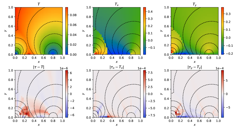
Figure 5: A test problem with two point sources. The domain is $\Omega=[0,1]^{2}$ discretized into a $33\times 33$ grid. The top row contains computed values and the bottom row contains signed errors. We overlay several contours of the numerically computed eikonal, $T$, for context. The two point sources are separated by a shockline, which is accurately localized even for this extremely coarse mesh. E.g., if we compared values of $T_{x}$ or $T_{y}$ on the “wrong” side of the shockline, we would observe $O(1)$ error. Left: $T$. Middle: $T_{x}$. Right: $T_{y}$.

Two point sources

We consider a linear speed function:

(66) $$c(\boldsymbol{x})=\frac{1}{s(\boldsymbol{x})}=2+5x_{1}+20x_{2},$$

with point sources located at $\boldsymbol{x}_{0}=(0,0)$ and $\boldsymbol{x}_{1}=(0.8,0)$. This is the same problem considered in Figure 4 of Qi and Vladimirsky [31]. We use (62) to compute the groundtruth eikonal for each point source. If we let $\tau_{0}$ and $\tau_{1}$ denote the eikonals for each point source problem considered individually, then the combined eikonal is:

(67) $$\tau(\boldsymbol{x})=\min(\tau_{0}(\boldsymbol{x}),\tau_{1}(\boldsymbol{x})).$$

We can easily see that all derivatives of $\tau$ are undefined on the shockline, where $\tau_{0}\equiv\tau_{1}$. However, away from the shockline, the derivatives are well-defined and smooth: if $j=\operatorname{arg}\min_{i}\tau_{i}(\boldsymbol{x})$, then $D\tau\equiv D\tau_{j}$. We solve this problem on $\Omega=[0,1]^{2}$, so that $\Omega_{h}$ is a grid with $N=33$ nodes in each direction. The results are shown in Figure 5.

For this problem, we note that the shockline is localized sufficiently well: all nodes $\boldsymbol{x}\in\Omega_{h}$ are on the correct side, so that when we compute the errors, each nodal value is compared with the correct branch of $\tau=\min(\tau_{0},\tau_{1})$. Note the use of an extremely coarse mesh. The mesh used here is coarser than any mesh used in Qi and Vladimirsky’s Figure 4, but the eikonal achieves a smaller maximum error than all of their test problems.

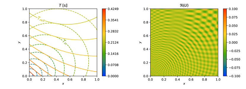
Figure 6: A single reflection from a wall in a semi-infinite domain for $\omega=1000$ (we consider only the top edge of the boundary to be reflecting). Left: $T$ for the incident and reflected fields. The reflected field satisfies a specular reflection condition along the edge of the domain. Right: the real part of the approximation to the solution of the Helmholtz equation so obtained, given by (74).

A single reflection

We additionally include a simple test for computing multiple arrivals. For the linear speed function:

(68) $$c(\boldsymbol{x})=\frac{1}{s(\boldsymbol{x})}=2+5x_{1}+7x_{2},$$

we solve (1) on $\Omega=[0,1]^{2}$, discretized into $N=101$ nodes in each direction. We place a point source at $\boldsymbol{x}=(0,0)$ and compute the eikonal, which we denote $\tau_{\operatorname{in}}$. We then restrict $\tau_{\operatorname{in}}$ and $\nabla\tau_{\operatorname{in}}$ (after reflection) to the set $\Gamma=[0,1]\times\{1\}$ (the top edge of the domain), and solve the reflected eikonal equation:

(69) $$\|\nabla\tau_{\operatorname{refl}}(\boldsymbol{x})\| =s(\boldsymbol{x}), \boldsymbol{x}\in\Omega,$$

(70) $$\tau_{\operatorname{refl}}(\boldsymbol{x}) =\tau_{\operatorname{in}}(\boldsymbol{x}), \boldsymbol{x}\in\Gamma,$$

(71) $$\left.\frac{\partial\tau_{\operatorname{refl}}}{\partial x}\right|_{\boldsymbol{x}} =\left.\frac{\partial\tau_{\operatorname{in}}}{\partial x}\right|_{\boldsymbol{x}}, \boldsymbol{x}\in\Gamma,$$

(72) $$\left.\frac{\partial\tau_{\operatorname{refl}}}{\partial y}\right|_{\boldsymbol{x}} =-\left.\frac{\partial\tau_{\operatorname{in}}}{\partial y}\right|_{\boldsymbol{x}}, \boldsymbol{x}\in\Gamma.$$

Note the minus sign in (72). This corresponds to a specular reflection from the “wall” $\Gamma$. After we compute $T_{\operatorname{in}}$ and $T_{\operatorname{refl}}$ numerically, we can then compute the geometric spreading $J_{\operatorname{in}}$ and reflected geometric spreading $J_{\operatorname{refl}}$. Since the reflecting set is flat, we can use the boundary condition [29]:

(73) $$J_{\operatorname{refl}}(\boldsymbol{x})=J_{\operatorname{in}}(\boldsymbol{x}),\qquad\boldsymbol{x}\in\Gamma.$$

Afterwards, we use (59) to obtain:

(74) $$U(\boldsymbol{x})=A_{\operatorname{in}}(\boldsymbol{x})\exp(-i\omega T_{\operatorname{in}}(\boldsymbol{x}))+A_{\operatorname{refl}}(\boldsymbol{x})\exp(-i\omega T_{\operatorname{refl}}(\boldsymbol{x})).$$

In Figure 6, we plot $T_{\operatorname{in}}$, $T_{\operatorname{out}}$, and the real part of $U$.

8.2 Experimental results

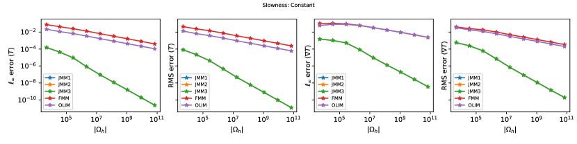
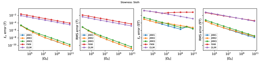
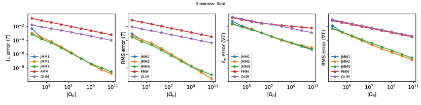
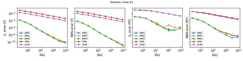
Figure 7: Plots comparing domain size ($|\Omega_{h}|$) and $\ell_{\infty}$ and RMS errors for $T$ and $\nabla T$.

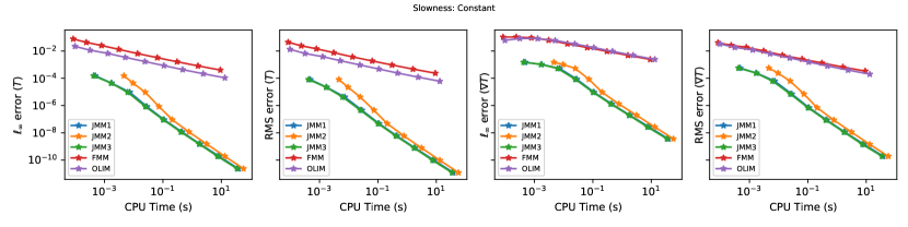
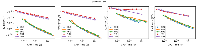
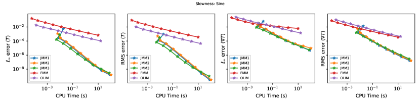
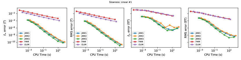
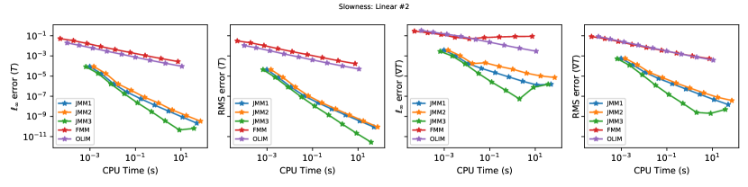
Figure 8: Plots comparing CPU runtime in seconds and errors.

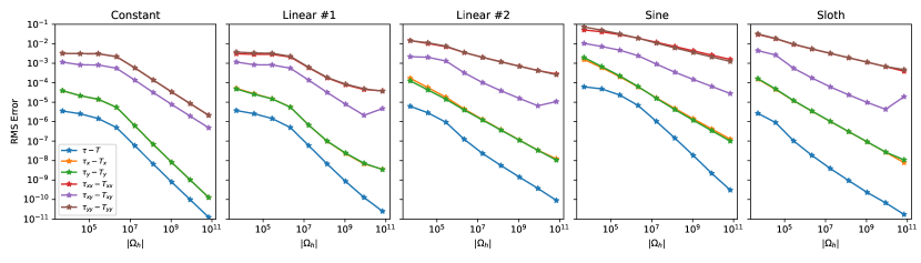
Figure 9: Domain size vs. RMS error for JMM4.

	JMM	$E_{\mbox{max}}(T)$	$E_{\mbox{RMS}}(T)$	$E_{\mbox{max}}(\nabla T)$	$E_{\mbox{RMS}}(\nabla T)$
Constant	#1	2.87	2.87	2.28	2.72
	#2	2.87	2.87	2.28	2.72
	#3	2.87	2.87	2.28	2.72
Linear #1	#1	2.77	2.85	2.14	2.52
	#2	2.77	2.85	1.70	2.48
	#3	2.86	2.87	2.28	2.73
Linear #2	#1	2.48	2.52	1.70	1.97
	#2	2.38	2.52	1.16	1.88
	#3	3.03	3.03	2.70	3.02
Sine	#1	2.76	2.57	1.77	2.09
	#2	2.51	2.46	1.58	1.94
	#3	2.37	2.38	1.54	1.79
Sloth	#1	2.39	2.48	1.49	1.84
	#2	2.37	2.47	0.87	1.73
	#3	2.15	2.21	1.47	1.76

Table 1: The order of convergence $p$ for each combination of test problems and solvers, computed for different types of errors and fit as $Ch^{p}$.

	$\tau-T$	$\tau_{x}-T_{x}$	$\tau_{y}-T_{y}$	$\tau_{xx}-T_{xx}$	$\tau_{xy}-T_{xy}$	$\tau_{yy}-T_{yy}$
Constant	3.09	3.11	3.11	2.01	2.05	2.01
Linear #1	2.99	2.43	2.40	1.39	2.01	1.39
Linear #2	2.10	1.76	1.72	0.77	1.25	0.77
Sine	2.91	1.80	1.89	0.73	1.31	0.80
Sloth	2.03	1.76	1.75	0.75	1.33	0.76

Table 2: The order of convergence $p$ for JMM4 for each component of the total 2-jet of $\tau$, computed from least squares fits of the RMS error. The fits only incorporate the 4th through the 8th problem sizes to avoid artifacts for small and large problem sizes. See Figure 9.

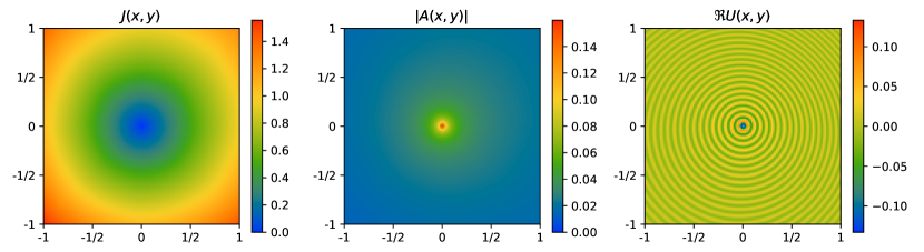
Figure 11: Plots related to computing the amplitude and a numerical approximation to the solution to $(\Delta+\omega^{2}s(\boldsymbol{x})^{2})u(\boldsymbol{x})=\delta(\boldsymbol{x})$, denoted $U(\boldsymbol{x})$ for the Linear #1 test problem. Left: the geometric spreading. Middle: the amplitude function. Right: the numerical solution $U$.

The results of our numerical experiments evaluating the JMMs described in Section 4 are presented in Table 1 and Figures 7 and 8. The numerical tests for JMM4, which uses cell marching, are given in Table 2 and Figures 9 and 10. An example where the geometric spreading and amplitude are computed using cell marching method is shown in Figure 11.

For more benign choices of $s$, the errors generally convergence with $O(h^{3})$ accuracy for $T$ and $O(h^{2})$ accuracy for $\nabla T$ in the RMS error. For the special case of $s\equiv 1$, the gradients also converge with nearly $O(h^{3})$ accuracy. For more challenging nonlinear choices of $s$, the eikonal converges with somewhere between $O(h^{2})$ and $O(h^{3})$ accuracy, while the gradient converges with nearly $O(h^{2})$ accuracy.

We note that in some cases the gradient begins to diverge for large problem sizes. This occurs because our tolerance for minimizing $F$ is not small enough, and also because $\nabla^{2}F$ is $O(h)$. For our application, our goal is to save memory and compute time by using a higher-order solver; it is unlikely we would solve problems with such a fine discretization in practice. At the same time, choosing the tolerance for numerical minimization based on $h$ is of interest—partly to see how much time can be saved for coarser problems, but also to determine to what extent the full order of convergence can be maintained using different floating point precisions.

The JMMs using cubic approximations for $\boldsymbol{\varphi}$ tend to perform better than those using quadratic approximations when $s$ is nonlinear and the characteristics of (1) are not circular arcs. When $s$ corresponds to a linear speed of sound, the JMMs with quadratic $\boldsymbol{\varphi}$ are a suitable choice, generally outperforming the “cubic $\boldsymbol{\varphi}$” solvers, exhibiting cubically (or nearly cubically) convergent RMS errors in $T$ and $\nabla T$. This is a useful finding since the simplified solver requires fewer floating-point operations per update, and since linear speed of sound profiles (e.g., as a function of a linear temperature profile) are a frequently occurring phenomenon in room acoustics.

9 Online Package

To recreate our results, to experiment with these solvers, and to understand their workings, a package has been made available online on GitHub at https://github.com/sampotter/jmm/tree/jmm-sisc-figures. Details explaining how to obtain this package and the collect the results are available at this link.

10 Conclusion

We have presented a family of semi-Lagrangian label-setting methods (à la the fast marching method) which are high-order and compact, which we refer to as jet marching methods (JMMs). We examine a variety of approaches to formulating one of these solvers, and in 2D, provide extensive numerical results demonstrating the efficacy of these approaches. We show how a form of “adaptive” cell-marching can be done which is compatible with our stencil compactness requirements, although this scheme no longer displays optimal locality.

Our solvers are motivated by problems involving repeatedly solving the eikonal equation in complicated domains where:

• time and memory savings via the use of high-order solvers,

• high-order local knowledge of characteristic directions,

• and compactness of the solver’s “stencil” (the neighborhood over which the semi-Lagrangian updates require information)

is paramount. In particular, our goal is to parametrize the multipath eikonal in a complicated polyhedral domain in a work-efficient manner. This solver is a necessary ingredient for carrying out this task.

We will be continue to work along the following directions:

• Extension to regular grids in 3D, which should be straightforward and yield considerable savings over existing approaches, and extension to unstructured simplex meshes in 2D and 3D. Especially in 3D, this problem is more complicated, requiring the computation of “causal stencils” [22, 41].

• A rigorous proof of convergence for the solvers developed in this work, including a careful investigation of the conditions resulting in cubic convergence for both the eikonal and its gradient as observed in the case of constant and linear speed functions.

11 Acknowledgments

This work was partially supported by NSF Career Grant DMS1554907 and MTECH Grant No. 6205. We thank Prof. Ramani Duraiswami for the illuminating discussions and trenchant observations provided throughout the course of this work.

References

- [1] P.-A. Absil, R. Mahony, and R. Sepulchre, Optimization algorithms on matrix manifolds, Princeton University Press, 2009.
- [2] J. B. Allen and D. A. Berkley, Image method for efficiently simulating small-room acoustics, The Journal of the Acoustical Society of America, 65 (1979), pp. 943–950.
- [3] G. S. Ávila and J. B. Keller, The high-frequency asymptotic field of a point source in an inhomogeneous medium, Communications on Pure and Applied mathematics, 16 (1963), pp. 363–381.
- [4] V. M. Babich and N. Y. Kirpichnikova, The boundary-layer method in diffraction problems, vol. 3, Springer, 1979.
- [5] J.-D. Benamou, Big ray tracing: Multivalued travel time field computation using viscosity solutions of the eikonal equation, Journal of Computational Physics, 128 (1996), pp. 463–474.
- [6] J.-D. Benamou, Multivalued solution and viscosity solutions of the eikonal equation. 1997.
- [7] J.-D. Benamou, An introduction to eulerian geometrical optics (1992–2002), Journal of scientific computing, 19 (2003), pp. 63–93.
- [8] J.-D. Benamou, S. Luo, and H. Zhao, A compact upwind second order scheme for the eikonal equation, Journal of Computational Mathematics, (2010), pp. 489–516.
- [9] F. Bornemann and C. Rasch, Finite-element discretization of static hamilton-jacobi equations based on a local variational principle, Computing and Visualization in Science, 9 (2006), pp. 57–69.
- [10] P. Brunet, Increasing the smoothness of bicubic spline surfaces, Computer Aided Geometric Design, 2 (1985), pp. 157–164.
- [11] M. K. Cameron, Jet marching method, September 2020, https://youtu.be/Ze9AeDbaDVM.
- [12] A. Chacon and A. Vladimirsky, Fast two-scale methods for eikonal equations, SIAM Journal on Scientific Computing, 34 (2012), pp. A547–A578.
- [13] A. Chandak, C. Lauterbach, M. Taylor, Z. Ren, and D. Manocha, Ad-frustum: Adaptive frustum tracing for interactive sound propagation, IEEE Transactions on Visualization and Computer Graphics, 14 (2008), pp. 1707–1722.
- [14] D. L. Chopp, Some improvements of the fast marching method, SIAM Journal on Scientific Computing, 23 (2001), pp. 230–244.
- [15] G. Farin, Curves and surfaces for computer-aided geometric design: a practical guide, Elsevier, 2014.
- [16] M. S. Floater, Chordal cubic spline interpolation is fourth-order accurate, IMA Journal of Numerical Analysis, 26 (2006), pp. 25–33.
- [17] S. Fomel, S. Luo, and H. Zhao, Fast sweeping method for the factored eikonal equation, Journal of Computational Physics, 228 (2009), pp. 6440–6455.
- [18] J. V. Gómez, D. Alvarez, S. Garrido, and L. Moreno, Fast methods for eikonal equations: an experimental survey, IEEE Access, (2019).
- [19] A. Griewank and A. Walther, Evaluating derivatives: principles and techniques of algorithmic differentiation, vol. 105, Siam, 2008.
- [20] H. Hagen and G. Schulze, Automatic smoothing with geometric surface patches, Computer Aided Geometric Design, 4 (1987), pp. 231–235.
- [21] J. B. Keller, Geometrical theory of diffraction, JOSA, 52 (1962), pp. 116–130.
- [22] R. Kimmel and J. A. Sethian, Computing geodesic paths on manifolds, Proceedings of the national academy of Sciences, 95 (1998), pp. 8431–8435.
- [23] R. G. Kouyoumjian and P. H. Pathak, A uniform geometrical theory of diffraction for an edge in a perfectly conducting surface, Proceedings of the IEEE, 62 (1974), pp. 1448–1461.
- [24] S. Luo, J. Qian, and R. Burridge, High-order factorization based high-order hybrid fast sweeping methods for point-source eikonal equations, SIAM Journal on Numerical Analysis, 52 (2014), pp. 23–44.
- [25] J.-C. Nave, R. R. Rosales, and B. Seibold, A gradient-augmented level set method with an optimally local, coherent advection scheme, Journal of Computational Physics, 229 (2010), pp. 3802–3827.
- [26] R. D. Neidinger, Introduction to automatic differentiation and matlab object-oriented programming, SIAM review, 52 (2010), pp. 545–563.
- [27] F. E. Nicodemus, Directional reflectance and emissivity of an opaque surface, Applied optics, 4 (1965), pp. 767–775.
- [28] M. Popov, I. Pšenčík, and V. Červenỳ, Computation of ray amplitudes in inhomogeneous media with curved interfaces, Studia Geophysica et Geodaetica, 22 (1978), pp. 248–258.
- [29] M. M. Popov, Ray theory and Gaussian beam method for geophysicists, EDUFBA, 2002.
- [30] S. F. Potter and M. K. Cameron, Ordered line integral methods for solving the eikonal equation, Journal of Scientific Computing, 81 (2019), pp. 2010–2050.
- [31] D. Qi and A. Vladimirsky, Corner cases, singularities, and dynamic factoring, Journal of Scientific Computing, 79 (2019), pp. 1456–1476.
- [32] J. Qian, L. Yuan, Y. Liu, S. Luo, and R. Burridge, Babich’s expansion and high-order eulerian asymptotics for point-source helmholtz equations, Journal of Scientific Computing, 67 (2016), pp. 883–908.
- [33] N. Raghuvanshi and J. Snyder, Parametric wave field coding for precomputed sound propagation, ACM Transactions on Graphics (TOG), 33 (2014), p. 38.
- [34] N. Raghuvanshi and J. Snyder, Parametric directional coding for precomputed sound propagation, ACM Transactions on Graphics (TOG), 37 (2018), p. 108.
- [35] L. Savioja and U. P. Svensson, Overview of geometrical room acoustic modeling techniques, The Journal of the Acoustical Society of America, 138 (2015), pp. 708–730.
- [36] C. Schissler, R. Mehra, and D. Manocha, High-order diffraction and diffuse reflections for interactive sound propagation in large environments, ACM Transactions on Graphics (TOG), 33 (2014), p. 39.
- [37] B. Seibold, J.-C. Nave, and R. R. Rosales, Jet schemes for advection problems, arXiv preprint arXiv:1101.5374, (2011).
- [38] J. A. Sethian, A fast marching level set method for monotonically advancing fronts, Proceedings of the National Academy of Sciences, 93 (1996), pp. 1591–1595.
- [39] J. A. Sethian, Fast marching methods, SIAM review, 41 (1999), pp. 199–235.
- [40] J. A. Sethian, Level set methods and fast marching methods: evolving interfaces in computational geometry, fluid mechanics, computer vision, and materials science, vol. 3, Cambridge University Press, 1999.
- [41] J. A. Sethian and A. Vladimirsky, Fast methods for the Eikonal and related Hamilton–Jacobi equations on unstructured meshes, Proceedings of the National Academy of Sciences, 97 (2000), pp. 5699–5703.
- [42] J. A. Sethian and A. Vladimirsky, Ordered upwind methods for static Hamilton–Jacobi equations: theory and algorithms, SIAM Journal on Numerical Analysis, 41 (2003), pp. 325–363.
- [43] G. E. Shilov and R. A. Silverman, Linear Algebra, Prentice-Hall, 1971.
- [44] M. M. Slotnick, Lessons in seismic computing: A memorial to the author, Society of exploration geophysicists, 1959.
- [45] J. Stoer and R. Bulirsch, Introduction to numerical analysis, vol. 12, Springer Science & Business Media, 2013.
- [46] J. N. Tsitsiklis, Efficient algorithms for globally optimal trajectories, IEEE Transactions on Automatic Control, 40 (1995), pp. 1528–1538.
- [47] R. Versteeg, The marmousi experience: Velocity model determination on a synthetic complex data set, The Leading Edge, 13 (1994), pp. 927–936.
- [48] T. Xiong, M. Zhang, Y.-T. Zhang, and C.-W. Shu, Fast sweeping fifth order WENO scheme for static Hamilton-Jacobi equations with accurate boundary treatment, Journal of Scientific Computing, 45 (2010), pp. 514–536.
- [49] S. Yang, S. F. Potter, and M. K. Cameron, Computing the quasipotential for nongradient SDEs in 3D, Journal of Computational Physics, 379 (2019), pp. 325–350.
- [50] Y.-T. Zhang, H.-K. Zhao, and J. Qian, High order fast sweeping methods for static Hamilton-Jacobi equations, Journal of Scientific Computing, 29 (2006), pp. 25–56.
- [51] H. Zhao, A fast sweeping method for eikonal equations, Mathematics of computation, 74 (2005), pp. 603–627.