Revisit the tetraquark candidates in the $J/\psi J/\psi$ mass spectrum

Zhi-Gang Wang 111E-mail: zgwang@aliyun.com.

Department of Physics, North China Electric Power University, Baoding 071003, P. R. China

Abstract

In this article, we introduce a relative P-wave to construct the doubly-charm axialvector diquark operator, then take the doubly-charm axialvector (anti)diquark operator as the basic constituent to construct the scalar and tensor tetraquark currents to study the scalar, axialvector and tensor fully-charm tetraquark states with the QCD sum rules. We observe that the ground state $\tilde{A}\tilde{A}$ type tetraquark states and the first radial excited states of the $AA$ type tetraquark states have almost degenerated masses, where the $\tilde{A}$ and $A$ stand for the diquark operators with and without the relative P-wave respectively, the broad structure above the $J/\psi J/\psi$ threshold maybe consist of several diquark-antidiquark type fully-charm tetraquark states.

PACS number: 12.39.Mk, 12.38.Lg

Key words: Tetraquark states, QCD sum rules

1 Introduction

In the constituent quark models, we usually classify the hadrons into conventional mesons and baryons, and exotic tetraquark states, pentaquark states and hexaquark states, etc. The $X(3872)$, the first exotic candidate observed in 2003 by the Belle collaboration [1], has hidden-charm, but cannot be fitted into any radial or orbital excitation of the charmonium, it should have more complicated structure than a mere $c\bar{c}$ pair. The exotic states provide a unique environment to explore the strong interaction, which governs the dynamics of the quarks and gluons, and the confinement mechanism. All the hadrons listed in The Review of Particle Physics to date contain two heavy valence quarks at most [2], whereas many QCD-motivated phenomenological models permit the existence of tetraquark states consisting of four heavy valence quarks, the fully-heavy tetraquark states have attracted much attentions in recent years and have been studied extensively [3, 4, 5, 6, 7, 8].

Recently, the LHCb collaboration studied the $J/\psi J/\psi$ invariant mass spectrum using proton-proton collision data at centre-of-mass energies of $\sqrt{s}=$7, 8 and 13 TeV recorded by the LHCb experiment corresponding to an integrated luminosity of $9\,\rm{fb}^{-1}$, and observed a narrow resonance structure around $6.9\,\rm{GeV}$ and a broad structure just above the $J/\psi J/\psi$ mass with global significances of more than five standard deviations [9]. The Breit-Wigner mass and width of the $X(6900)$ are

$\displaystyle M_{X}$ $\displaystyle=$ $\displaystyle 6905\pm 11\pm 7\,\rm{MeV}\,,$
$\displaystyle\Gamma_{X}$ $\displaystyle=$ $\displaystyle 80\pm 19\pm 33\,\rm{MeV}\,,$ (1)

assuming no interference with the nonresonant single-parton scattering continuum. When assuming the nonresonant single-parton scattering continuum interferes with the broad structure close to the $J/\psi J/\psi$ mass threshold, the Breit-Wigner mass and width are changed to

$\displaystyle M_{X}$ $\displaystyle=$ $\displaystyle 6886\pm 11\pm 11\rm{MeV}\,,$
$\displaystyle\Gamma_{X}$ $\displaystyle=$ $\displaystyle 168\pm 33\pm 69\,\rm{MeV}\,.$ (2)

Both the narrow and broad resonance structures are observed in the $J/\psi J/\psi$ invariant mass spectrum, such structures are naturally assigned to have the valence quarks or constituent quarks $c\bar{c}c\bar{c}$, which makes them the first fully-heavy exotic multiquark candidates claimed experimentally to date, their observations have revitalized the investigations of multiquark resonances made of heavy quarks and heavy antiquarks [10, 11, 12, 13]. It is a very important step in investigations of the heavy hadrons, after discoveries of the charmonium $c\bar{c}$ in 1974, and the charmed mesons $c\bar{q}$ and baryons $cqq$ in the subsequent years; the bottomonium $b\bar{b}$ in 1977, and the bottom mesons $b\bar{q}$ and baryons $bqq$ in the subsequent years; the $B_{c}$ in 1996 at the Fermilab Tevatron collider; and the double-charm baryons $ccq$ in 2017 by the LHCb collaboration [2].

In spite of a large body of experimental information accumulated on the exotic hadrons, we have never reached consensus on the way the valence quarks are organized inside them, the diquark-antidiquark type, color-singlet-color-singlet type, or other type quark structures? In the present case, there are no known color-singlet light mesons can be exchanged between two charmonium states to produce binding energies or final-state interactions. The thresholds of the charmonium pairs $\eta_{c}\eta_{c}$, $J/\psi J/\psi$, $\chi_{c0}\chi_{c0}$, $\chi_{c1}\chi_{c1}$, $h_{c}h_{c}$ and $\chi_{c2}\chi_{c2}$ are $5.97\,\rm{GeV}$, $6.19\,\rm{GeV}$, $6.83\,\rm{GeV}$, $7.02\,\rm{GeV}$, $7.05\,\rm{GeV}$ and $7.11\,\rm{GeV}$ respectively from the Particle Data Group [2]. The $X(6900)$ lies about $700\,\rm{MeV}$ above the $J/\psi J/\psi$ threshold, and in the vicinity of the $\chi_{c0}\chi_{c0}$ and $\chi_{c1}\chi_{c0}$ thresholds, it is very difficult to produce such a strong resonance structure through the threshold rescattering mechanism. As a result, the most general models for the fully-heavy four-quark states resort to the diquark-antidiquark configurations, the attractive interactions between the two heavy quarks or antiquarks should dominate at the short distance and favor forming the genuine diquark-antidiquark type tetraquark states rather than the loosely-bound tetraquark molecular states. Needless to say, determining the spin-parity of the resonances is in the first priority.

More precisely, the attractive (repulsive) interaction in the antisymmetric (symmetric) color antitriplet (sextet) channel originates from the one-gluon exchange favors (disfavors) formation of the diquarks in the color antitriplet (sextet). We prefer the diquarks in the color antitriplet to the diquarks in the color sextet in constructing the tetraquark current operators. The diquark operators $\varepsilon^{ijk}q^{T}_{j}C\Gamma q^{\prime}_{k}$ have five structures in Dirac spinor space, where the $i$, $j$ and $k$ are color indexes, $C\Gamma=C\gamma_{5}$, $C$, $C\gamma_{\mu}\gamma_{5}$, $C\gamma_{\mu}$ and $C\sigma_{\mu\nu}$ for the scalar, pseudoscalar, vector, axialvector and tensor diquarks, respectively. The favorite diquark configurations are the scalar ($C\gamma_{5}$) and axialvector ($C\gamma_{\mu}$) diquark states from the QCD sum rules [14, 15]. The double-heavy diquark operators $\varepsilon^{ijk}Q^{T}_{j}C\gamma_{5}Q_{k}$ cannot exist due to the Fermi-Dirac statistics. In previous work, we took the doubly-heavy diquark operators $\varepsilon^{ijk}Q^{T}_{j}C\gamma_{\mu}Q_{k}$ ($A$) as basic constituents to construct the scalar and tensor currents to study the scalar, axialvector, vector, tensor tetraquark states and their radial excited states with the QCD sum rules [4, 11]. Now we introduce the explicit P-wave to construct the axialvector doubly-heavy diquark operators $\varepsilon^{ijk}Q^{T}_{j}C\gamma_{5}\stackrel{{\scriptstyle\leftrightarrow}}{{\partial}}_{\mu}Q_{k}$ ($\tilde{A}$), which can exist due to the Fermi-Dirac statistics, the derivative $\stackrel{{\scriptstyle\leftrightarrow}}{{\partial}}_{\mu}=\stackrel{{\scriptstyle\rightarrow}}{{\partial}}_{\mu}-\stackrel{{\scriptstyle\leftarrow}}{{\partial}}_{\mu}$ embodies the P-wave effect.

In this article, we take the axialvector diquark operator $\tilde{A}$ as the basic constituent, construct the $\tilde{A}\tilde{A}$ type scalar and tensor tetraquark currents to study the mass spectrum of the ground states of the scalar, axialvector and tensor fully-charm tetraquark states with the QCD sum rules, and try to make possible assignments of the LHCb’s new resonance structures.

The article is arranged as follows: we derive the QCD sum rules for the masses and pole residues of the $cc\bar{c}\bar{c}$ tetraquark states in section 2; in section 3, we present the numerical results and discussions; section 4 is reserved for our conclusion.

2 QCD sum rules for the $\tilde{A}\tilde{A}$ type tetraquark states

We write down the two-point correlation functions $\Pi(p)$ and Πμ​ν​α​β​(p)subscriptΞ πœ‡πœˆπ›Όπ›½π‘\Pi_{\mu\nu\alpha\beta}(p) in the QCD sum rules firstly,

$\displaystyle\Pi(p)$ $\displaystyle=$ $\displaystyle i\int d^{4}xe^{ip\cdot x}\langle 0|T\left\{J(x)J^{\dagger}(0)\right\}|0\rangle\,,$
Πμ​ν​α​β​(p)subscriptΞ πœ‡πœˆπ›Όπ›½π‘\displaystyle\Pi_{\mu\nu\alpha\beta}(p) $\displaystyle=$ $\displaystyle i\int d^{4}xe^{ip\cdot x}\langle 0|T\left\{J_{\mu\nu}(x)J_{\alpha\beta}^{\dagger}(0)\right\}|0\rangle\,,$ (3)

where $J_{\mu\nu}(x)=J^{1}_{\mu\nu}(x)$, $J^{2}_{\mu\nu}(x)$,

$\displaystyle J(x)$ $\displaystyle=$ $\displaystyle\varepsilon^{ijk}\varepsilon^{imn}c^{Tj}(x)C\gamma_{5}\stackrel{{\scriptstyle\leftrightarrow}}{{\partial}}_{\mu}c^{k}(x)\,\bar{c}^{m}(x)\stackrel{{\scriptstyle\leftrightarrow}}{{\partial}}_{\nu}\gamma_{5}C\bar{c}^{Tn}(x)\,g^{\mu\nu}\,,$
$\displaystyle J^{1}_{\mu\nu}(x)$ $\displaystyle=$ $\displaystyle\varepsilon^{ijk}\varepsilon^{imn}\Big{\{}c^{Tj}(x)C\gamma_{5}\stackrel{{\scriptstyle\leftrightarrow}}{{\partial}}_{\mu}c^{k}(x)\,\bar{c}^{m}(x)\stackrel{{\scriptstyle\leftrightarrow}}{{\partial}}_{\nu}\gamma_{5}C\bar{c}^{Tn}(x)$
$\displaystyle-c^{Tj}(x)C\gamma_{5}\stackrel{{\scriptstyle\leftrightarrow}}{{\partial}}_{\nu}c^{k}(x)\,\bar{c}^{m}(x)\stackrel{{\scriptstyle\leftrightarrow}}{{\partial}}_{\mu}\gamma_{5}C\bar{c}^{Tn}(x)\Big{\}}\,,$
$\displaystyle J^{2}_{\mu\nu}(x)$ $\displaystyle=$ $\displaystyle\varepsilon^{ijk}\varepsilon^{imn}\Big{\{}c^{Tj}(x)C\gamma_{5}\stackrel{{\scriptstyle\leftrightarrow}}{{\partial}}_{\mu}c^{k}(x)\,\bar{c}^{m}(x)\stackrel{{\scriptstyle\leftrightarrow}}{{\partial}}_{\nu}\gamma_{5}C\bar{c}^{Tn}(x)$ (4)
$\displaystyle+c^{Tj}(x)C\gamma_{5}\stackrel{{\scriptstyle\leftrightarrow}}{{\partial}}_{\nu}c^{k}(x)\,\bar{c}^{m}(x)\stackrel{{\scriptstyle\leftrightarrow}}{{\partial}}_{\mu}\gamma_{5}C\bar{c}^{Tn}(x)\Big{\}}\,,$

the $i$, $j$, $k$, $m$, $n$ are color indexes, the $C$ is the charge conjugation matrix. We choose the tetraquark currents $J(x)$, $J^{1}_{\mu\nu}(x)$ and $J^{2}_{\mu\nu}(x)$ to interpolate the $J^{PC}=0^{++}$, $1^{+-}$ and $2^{++}$ diquark-antidiquark type tetraquark states, respectively.

At the hadron side, we insert a complete set of intermediate hadronic states with the same quantum numbers as the tetraquark current operators $J(x)$, $J^{1}_{\mu\nu}(x)$ and $J^{2}_{\mu\nu}(x)$ into the correlation functions $\Pi(p)$ and Πμ​ν​α​β​(p)subscriptΞ πœ‡πœˆπ›Όπ›½π‘\Pi_{\mu\nu\alpha\beta}(p) to obtain the hadronic representation [16, 17]. After isolating the ground state contributions of the scalar, axialvector and tensor fully-charm tetraquark states, we obtain the results,

$\displaystyle\Pi(p)$ $\displaystyle=$ $\displaystyle\frac{\lambda_{X}^{2}}{M^{2}_{X}-p^{2}}+\cdots\,\,,$ (5)
$\displaystyle=$ Ξ S​(p2),subscriptΠ𝑆superscript𝑝2\displaystyle\Pi_{S}(p^{2})\,,
Πμ​ν​α​β1​(p)subscriptsuperscriptΞ 1πœ‡πœˆπ›Όπ›½π‘\displaystyle\Pi^{1}_{\mu\nu\alpha\beta}(p) $\displaystyle=$ $\displaystyle\frac{\lambda_{Y^{+}}^{2}}{M_{Y^{+}}^{2}\left(M_{Y^{+}}^{2}-p^{2}\right)}\left(p^{2}g_{\mu\alpha}g_{\nu\beta}-p^{2}g_{\mu\beta}g_{\nu\alpha}-g_{\mu\alpha}p_{\nu}p_{\beta}-g_{\nu\beta}p_{\mu}p_{\alpha}+g_{\mu\beta}p_{\nu}p_{\alpha}+g_{\nu\alpha}p_{\mu}p_{\beta}\right)$ (6)
$\displaystyle+\frac{\lambda_{Y^{-}}^{2}}{M_{Y^{-}}^{2}\left(M_{Y^{-}}^{2}-p^{2}\right)}\left(-g_{\mu\alpha}p_{\nu}p_{\beta}-g_{\nu\beta}p_{\mu}p_{\alpha}+g_{\mu\beta}p_{\nu}p_{\alpha}+g_{\nu\alpha}p_{\mu}p_{\beta}\right)+\cdots\,\,,$
$\displaystyle=$ Ξ ~A​(p2)​(p2​gμ​α​gΞ½β€‹Ξ²βˆ’p2​gμ​β​gΞ½β€‹Ξ±βˆ’gμ​α​pν​pΞ²βˆ’gν​β​pμ​pΞ±+gμ​β​pν​pΞ±+gν​α​pμ​pΞ²)subscript~Π𝐴superscript𝑝2superscript𝑝2subscriptπ‘”πœ‡π›Όsubscriptπ‘”πœˆπ›½superscript𝑝2subscriptπ‘”πœ‡π›½subscriptπ‘”πœˆπ›Όsubscriptπ‘”πœ‡π›Όsubscriptπ‘πœˆsubscript𝑝𝛽subscriptπ‘”πœˆπ›½subscriptπ‘πœ‡subscript𝑝𝛼subscriptπ‘”πœ‡π›½subscriptπ‘πœˆsubscript𝑝𝛼subscriptπ‘”πœˆπ›Όsubscriptπ‘πœ‡subscript𝑝𝛽\displaystyle\widetilde{\Pi}_{A}(p^{2})\left(p^{2}g_{\mu\alpha}g_{\nu\beta}-p^{2}g_{\mu\beta}g_{\nu\alpha}-g_{\mu\alpha}p_{\nu}p_{\beta}-g_{\nu\beta}p_{\mu}p_{\alpha}+g_{\mu\beta}p_{\nu}p_{\alpha}+g_{\nu\alpha}p_{\mu}p_{\beta}\right)
+Ξ ~V​(p2)​(βˆ’gμ​α​pν​pΞ²βˆ’gν​β​pμ​pΞ±+gμ​β​pν​pΞ±+gν​α​pμ​pΞ²).subscript~Π𝑉superscript𝑝2subscriptπ‘”πœ‡π›Όsubscriptπ‘πœˆsubscript𝑝𝛽subscriptπ‘”πœˆπ›½subscriptπ‘πœ‡subscript𝑝𝛼subscriptπ‘”πœ‡π›½subscriptπ‘πœˆsubscript𝑝𝛼subscriptπ‘”πœˆπ›Όsubscriptπ‘πœ‡subscript𝑝𝛽\displaystyle+\widetilde{\Pi}_{V}(p^{2})\left(-g_{\mu\alpha}p_{\nu}p_{\beta}-g_{\nu\beta}p_{\mu}p_{\alpha}+g_{\mu\beta}p_{\nu}p_{\alpha}+g_{\nu\alpha}p_{\mu}p_{\beta}\right)\,.
Πμ​ν​α​β2​(p)subscriptsuperscriptΞ 2πœ‡πœˆπ›Όπ›½π‘\displaystyle\Pi^{2}_{\mu\nu\alpha\beta}(p) $\displaystyle=$ $\displaystyle\frac{\lambda_{X}^{2}}{M_{X}^{2}-p^{2}}\left(\frac{\widetilde{g}_{\mu\alpha}\widetilde{g}_{\nu\beta}+\widetilde{g}_{\mu\beta}\widetilde{g}_{\nu\alpha}}{2}-\frac{\widetilde{g}_{\mu\nu}\widetilde{g}_{\alpha\beta}}{3}\right)+\cdots\,\,,$ (7)
$\displaystyle=$ Ξ T​(p2)​(g~μ​α​g~ν​β+g~μ​β​g~ν​α2βˆ’g~μ​ν​g~α​β3)+β‹―,subscriptΠ𝑇superscript𝑝2subscript~π‘”πœ‡π›Όsubscript~π‘”πœˆπ›½subscript~π‘”πœ‡π›½subscript~π‘”πœˆπ›Ό2subscript~π‘”πœ‡πœˆsubscript~𝑔𝛼𝛽3β‹―\displaystyle\Pi_{T}(p^{2})\left(\frac{\widetilde{g}_{\mu\alpha}\widetilde{g}_{\nu\beta}+\widetilde{g}_{\mu\beta}\widetilde{g}_{\nu\alpha}}{2}-\frac{\widetilde{g}_{\mu\nu}\widetilde{g}_{\alpha\beta}}{3}\right)+\cdots\,\,,

where $\widetilde{g}_{\mu\nu}=g_{\mu\nu}-\frac{p_{\mu}p_{\nu}}{p^{2}}$, the pole residues $\lambda_{X}$ and $\lambda_{Y}$ are defined by

$\displaystyle\langle 0|J(0)|X(p)\rangle$ $\displaystyle=$ $\displaystyle\lambda_{X}\,,$
$\displaystyle\langle 0|J^{1}_{\mu\nu}(0)|Y^{+}(p)\rangle$ $\displaystyle=$ $\displaystyle\frac{\lambda_{Y^{+}}}{M_{Y^{+}}}\,\varepsilon_{\mu\nu\alpha\beta}\,\varepsilon^{\alpha}p^{\beta}\,,$
$\displaystyle\langle 0|J^{1}_{\mu\nu}(0)|Y^{-}(p)\rangle$ $\displaystyle=$ $\displaystyle\frac{\lambda_{Y^{-}}}{M_{Y^{-}}}\left(\varepsilon_{\mu}p_{\nu}-\varepsilon_{\nu}p_{\mu}\right)\,,$
$\displaystyle\langle 0|J^{2}_{\mu\nu}(0)|X(p)\rangle$ $\displaystyle=$ $\displaystyle\lambda_{X}\,\varepsilon_{\mu\nu}\,,$ (8)

the superscripts $\pm$ on the $Y$ stand for the parity of the tetraquark states, the $\varepsilon_{\mu}$ and $\varepsilon_{\mu\nu}$ are the polarization vectors of the axialvector, vector and tensor tetraquark states, respectively. In Ref.[18], we assign the $Z_{c}(3900)$ to be an axialvector tetraquark state tentatively, and study it with the QCD sum rules in details by including the two-particle scattering state contributions and nonlocal effects between the diquark and antidiquark constituents. In calculations, we observe that the two-particle scattering state contributions cannot saturate the QCD sum rules at the hadron side, the contribution of the $Z_{c}(3900)$ plays an un-substitutable role, we can saturate the QCD sum rules with or without the two-particle scattering state contributions. The conclusion is applicable in the present case, and we neglect the contributions of the intermediate charmonium pairs, such as $\eta_{c}\eta_{c}$, $J/\psi J/\psi$, $\chi_{c0}\chi_{c0}$, etc.

We project out the axialvector and vector components Ξ ~A​(p2)subscript~Π𝐴superscript𝑝2\widetilde{\Pi}_{A}(p^{2}) and Ξ ~V​(p2)subscript~Π𝑉superscript𝑝2\widetilde{\Pi}_{V}(p^{2}) by introducing the operators $P_{A}^{\mu\nu\alpha\beta}$ and $P_{V}^{\mu\nu\alpha\beta}$, respectively,

Ξ A​(p2)subscriptΠ𝐴superscript𝑝2\displaystyle\Pi_{A}(p^{2}) $\displaystyle=$ p2​Π~A​(p2)=PAμ​ν​α​β​Πμ​ν​α​β​(p),superscript𝑝2subscript~Π𝐴superscript𝑝2superscriptsubscriptπ‘ƒπ΄πœ‡πœˆπ›Όπ›½subscriptΞ πœ‡πœˆπ›Όπ›½π‘\displaystyle p^{2}\widetilde{\Pi}_{A}(p^{2})=P_{A}^{\mu\nu\alpha\beta}\Pi_{\mu\nu\alpha\beta}(p)\,,
Ξ V​(p2)subscriptΠ𝑉superscript𝑝2\displaystyle\Pi_{V}(p^{2}) $\displaystyle=$ p2​Π~V​(p2)=PVμ​ν​α​β​Πμ​ν​α​β​(p),superscript𝑝2subscript~Π𝑉superscript𝑝2superscriptsubscriptπ‘ƒπ‘‰πœ‡πœˆπ›Όπ›½subscriptΞ πœ‡πœˆπ›Όπ›½π‘\displaystyle p^{2}\widetilde{\Pi}_{V}(p^{2})=P_{V}^{\mu\nu\alpha\beta}\Pi_{\mu\nu\alpha\beta}(p)\,, (9)

where

$\displaystyle P_{A}^{\mu\nu\alpha\beta}$ $\displaystyle=$ $\displaystyle\frac{1}{6}\left(g^{\mu\alpha}-\frac{p^{\mu}p^{\alpha}}{p^{2}}\right)\left(g^{\nu\beta}-\frac{p^{\nu}p^{\beta}}{p^{2}}\right)\,,$
$\displaystyle P_{V}^{\mu\nu\alpha\beta}$ $\displaystyle=$ $\displaystyle\frac{1}{6}\left(g^{\mu\alpha}-\frac{p^{\mu}p^{\alpha}}{p^{2}}\right)\left(g^{\nu\beta}-\frac{p^{\nu}p^{\beta}}{p^{2}}\right)-\frac{1}{6}g^{\mu\alpha}g^{\nu\beta}\,.$ (10)

The vector tetraquark state $Y^{-}$ has negative parity, and should have an additional P-wave compared to the tetraquark states $X$ with the positive parity, and is beyond the present work as there are three P-waves.

It is straightforward but tedious to compute the operator product expansion in the deep Euclidean space $P^{2}=-p^{2}\to\infty$, then we obtain the QCD spectral densities through dispersion relation,

Ξ S/A/T​(p2)subscriptΠ𝑆𝐴𝑇superscript𝑝2\displaystyle\Pi_{S/A/T}(p^{2}) $\displaystyle=$ ∫16​mc2βˆžπ‘‘s​ρS/A/T​(s)sβˆ’p2,superscriptsubscript16superscriptsubscriptπ‘šπ‘2differential-d𝑠subscriptπœŒπ‘†π΄π‘‡π‘ π‘ superscript𝑝2\displaystyle\int_{16m_{c}^{2}}^{\infty}ds\frac{\rho_{S/A/T}(s)}{s-p^{2}}\,, (11)

where

ρS/A/T​(s)subscriptπœŒπ‘†π΄π‘‡π‘ \displaystyle\rho_{S/A/T}(s) $\displaystyle=$ Im​ΠS/A/T​(s)Ο€.ImsubscriptΞ π‘†π΄π‘‡π‘ πœ‹\displaystyle\frac{{\rm Im}\Pi_{S/A/T}(s)}{\pi}\,. (12)

We take the quark-hadron duality below the continuum thresholds $s_{0}$, and perform Borel transform in regard to the variable $P^{2}=-p^{2}$ to obtain the QCD sum rules:

$\displaystyle\lambda^{2}_{X/Y}\,\exp\left(-\frac{M^{2}_{X/Y}}{T^{2}}\right)$ $\displaystyle=$ ∫16​mc2s0𝑑sβ€‹βˆ«4​mc2(sβˆ’2​mc)2𝑑tβ€‹βˆ«4​mc2(sβˆ’t)2𝑑r​ρ​(s,t,r)​exp⁑(βˆ’sT2),superscriptsubscript16superscriptsubscriptπ‘šπ‘2subscript𝑠0differential-d𝑠superscriptsubscript4superscriptsubscriptπ‘šπ‘2superscript𝑠2subscriptπ‘šπ‘2differential-d𝑑superscriptsubscript4superscriptsubscriptπ‘šπ‘2superscript𝑠𝑑2differential-dπ‘ŸπœŒπ‘ π‘‘π‘Ÿπ‘ superscript𝑇2\displaystyle\int_{16m_{c}^{2}}^{s_{0}}ds\int_{4m_{c}^{2}}^{\left(\sqrt{s}-2m_{c}\right)^{2}}dt\int_{4m_{c}^{2}}^{\left(\sqrt{s}-\sqrt{t}\right)^{2}}dr\,\rho(s,t,r)\exp\left(-\frac{s}{T^{2}}\right)\,, (13)

where the QCD spectral densities ρ​(s,t,r)=ρS​(s,t,r)πœŒπ‘ π‘‘π‘ŸsubscriptπœŒπ‘†π‘ π‘‘π‘Ÿ\rho(s,t,r)=\rho_{S}(s,t,r), ρA​(s,t,r)subscriptπœŒπ΄π‘ π‘‘π‘Ÿ\rho_{A}(s,t,r) and ρT​(s,t,r)subscriptπœŒπ‘‡π‘ π‘‘π‘Ÿ\rho_{T}(s,t,r),

ρS​(s,t,r)subscriptπœŒπ‘†π‘ π‘‘π‘Ÿ\displaystyle\rho_{S}(s,t,r) $\displaystyle=$ λ​(s,t,r)​λ​(t,mc2,mc2)​λ​(r,mc2,mc2)3072​π6​(1βˆ’4​mc2t)​(1βˆ’4​mc2r)πœ†π‘ π‘‘π‘Ÿπœ†π‘‘superscriptsubscriptπ‘šπ‘2superscriptsubscriptπ‘šπ‘2πœ†π‘Ÿsuperscriptsubscriptπ‘šπ‘2superscriptsubscriptπ‘šπ‘23072superscriptπœ‹614superscriptsubscriptπ‘šπ‘2𝑑14superscriptsubscriptπ‘šπ‘2π‘Ÿ\displaystyle\frac{\sqrt{\lambda(s,t,r)\,\lambda(t,m_{c}^{2},m_{c}^{2})\,\lambda(r,m_{c}^{2},m_{c}^{2})}}{3072\pi^{6}}\left(1-\frac{4m_{c}^{2}}{t}\right)\left(1-\frac{4m_{c}^{2}}{r}\right)
(sβˆ’2​tβˆ’2​r+r2+t2+10​r​ts)𝑠2𝑑2π‘Ÿsuperscriptπ‘Ÿ2superscript𝑑210π‘Ÿπ‘‘π‘ \displaystyle\left(s-2t-2r+\frac{r^{2}+t^{2}+10rt}{s}\right)
+⟨αs​G​GΟ€βŸ©β€‹Ξ»β€‹(s,t,r)​λ​(r,mc2,mc2)288​π4​(1βˆ’4​mc2r)​mc2tβˆ’4​mc2​1t​(tβˆ’4​mc2)delimited-⟨⟩subscriptπ›Όπ‘ πΊπΊπœ‹πœ†π‘ π‘‘π‘Ÿπœ†π‘Ÿsuperscriptsubscriptπ‘šπ‘2superscriptsubscriptπ‘šπ‘2288superscriptπœ‹414superscriptsubscriptπ‘šπ‘2π‘Ÿsuperscriptsubscriptπ‘šπ‘2𝑑4superscriptsubscriptπ‘šπ‘21𝑑𝑑4superscriptsubscriptπ‘šπ‘2\displaystyle+\langle\frac{\alpha_{s}GG}{\pi}\rangle\frac{\sqrt{\lambda(s,t,r)\,\lambda(r,m_{c}^{2},m_{c}^{2})}}{288\pi^{4}}\left(1-\frac{4m_{c}^{2}}{r}\right)\frac{m_{c}^{2}}{t-4m_{c}^{2}}\frac{1}{\sqrt{t\left(t-4m_{c}^{2}\right)}}
$\displaystyle\left(4t+4r-2s-24m_{c}^{2}+\frac{12m_{c}^{2}(r+t)-2r^{2}-2t^{2}-2rt-15m_{c}^{4}}{s}\right.$
$\displaystyle\left.+\frac{12sm_{c}^{2}-24rm_{c}^{2}+30m_{c}^{4}}{t}+\frac{12r^{2}m_{c}^{2}-6rm_{c}^{4}}{st}+\frac{30rm_{c}^{4}-15sm_{c}^{4}}{t^{2}}-\frac{15r^{2}m_{c}^{4}}{st^{2}}\right)$
+⟨αs​G​GΟ€βŸ©β€‹Ξ»β€‹(s,t,r)​λ​(r,mc2,mc2)384​π4​(1βˆ’4​mc2r)​mc2t​(tβˆ’4​mc2)delimited-⟨⟩subscriptπ›Όπ‘ πΊπΊπœ‹πœ†π‘ π‘‘π‘Ÿπœ†π‘Ÿsuperscriptsubscriptπ‘šπ‘2superscriptsubscriptπ‘šπ‘2384superscriptπœ‹414superscriptsubscriptπ‘šπ‘2π‘Ÿsuperscriptsubscriptπ‘šπ‘2𝑑𝑑4superscriptsubscriptπ‘šπ‘2\displaystyle+\langle\frac{\alpha_{s}GG}{\pi}\rangle\frac{\sqrt{\lambda(s,t,r)\,\lambda(r,m_{c}^{2},m_{c}^{2})}}{384\pi^{4}}\left(1-\frac{4m_{c}^{2}}{r}\right)\frac{m_{c}^{2}}{\sqrt{t\left(t-4m_{c}^{2}\right)}}
$\displaystyle\left(-6+\frac{3t+6r-10m_{c}^{2}}{s}+\frac{3s-6r+20m_{c}^{2}}{t}+\frac{3r^{2}-4rm_{c}^{2}}{st}+\frac{20rm_{c}^{2}-10sm_{c}^{2}}{t^{2}}-\frac{10r^{2}m_{c}^{2}}{st^{2}}\right)$
+⟨αs​G​GΟ€βŸ©β€‹Ξ»β€‹(s,t,r)​λ​(r,mc2,mc2)256​π4​(1βˆ’4​mc2r)​1t​(tβˆ’4​mc2)delimited-⟨⟩subscriptπ›Όπ‘ πΊπΊπœ‹πœ†π‘ π‘‘π‘Ÿπœ†π‘Ÿsuperscriptsubscriptπ‘šπ‘2superscriptsubscriptπ‘šπ‘2256superscriptπœ‹414superscriptsubscriptπ‘šπ‘2π‘Ÿ1𝑑𝑑4superscriptsubscriptπ‘šπ‘2\displaystyle+\langle\frac{\alpha_{s}GG}{\pi}\rangle\frac{\sqrt{\lambda(s,t,r)\,\lambda(r,m_{c}^{2},m_{c}^{2})}}{256\pi^{4}}\left(1-\frac{4m_{c}^{2}}{r}\right)\frac{1}{\sqrt{t\left(t-4m_{c}^{2}\right)}}
$\displaystyle\left(s-2t-2r+4m_{c}^{2}+\frac{r^{2}+t^{2}-14rt-2tm_{c}^{2}+28rm_{c}^{2}-20m_{c}^{4}}{s}+\frac{4rm_{c}^{2}-2sm_{c}^{2}+40m_{c}^{4}}{t}\right.$
$\displaystyle\left.-\frac{2r^{2}m_{c}^{2}+8rm_{c}^{4}}{st}+\frac{40rm_{c}^{4}-20sm_{c}^{4}}{t^{2}}-\frac{20r^{2}m_{c}^{4}}{st^{2}}\right)\,,$ (14)
ρA​(s,t,r)subscriptπœŒπ΄π‘ π‘‘π‘Ÿ\displaystyle\rho_{A}(s,t,r) $\displaystyle=$ λ​(s,t,r)​λ​(t,mc2,mc2)​λ​(r,mc2,mc2)4608​π6​(1βˆ’4​mc2t)​(1βˆ’4​mc2r)πœ†π‘ π‘‘π‘Ÿπœ†π‘‘superscriptsubscriptπ‘šπ‘2superscriptsubscriptπ‘šπ‘2πœ†π‘Ÿsuperscriptsubscriptπ‘šπ‘2superscriptsubscriptπ‘šπ‘24608superscriptπœ‹614superscriptsubscriptπ‘šπ‘2𝑑14superscriptsubscriptπ‘šπ‘2π‘Ÿ\displaystyle\frac{\sqrt{\lambda(s,t,r)\,\lambda(t,m_{c}^{2},m_{c}^{2})\,\lambda(r,m_{c}^{2},m_{c}^{2})}}{4608\pi^{6}}\left(1-\frac{4m_{c}^{2}}{t}\right)\left(1-\frac{4m_{c}^{2}}{r}\right) (15)
(t+rβˆ’2​r2+2​t2βˆ’8​r​ts+(t+r)​(rβˆ’t)2s2)π‘‘π‘Ÿ2superscriptπ‘Ÿ22superscript𝑑28π‘Ÿπ‘‘π‘ π‘‘π‘Ÿsuperscriptπ‘Ÿπ‘‘2superscript𝑠2\displaystyle\left(t+r-\frac{2r^{2}+2t^{2}-8rt}{s}+\frac{(t+r)(r-t)^{2}}{s^{2}}\right)
+⟨αs​G​GΟ€βŸ©β€‹Ξ»β€‹(s,t,r)​λ​(r,mc2,mc2)864​π4​(1βˆ’4​mc2r)​mc2tβˆ’4​mc2​1t​(tβˆ’4​mc2)delimited-⟨⟩subscriptπ›Όπ‘ πΊπΊπœ‹πœ†π‘ π‘‘π‘Ÿπœ†π‘Ÿsuperscriptsubscriptπ‘šπ‘2superscriptsubscriptπ‘šπ‘2864superscriptπœ‹414superscriptsubscriptπ‘šπ‘2π‘Ÿsuperscriptsubscriptπ‘šπ‘2𝑑4superscriptsubscriptπ‘šπ‘21𝑑𝑑4superscriptsubscriptπ‘šπ‘2\displaystyle+\langle\frac{\alpha_{s}GG}{\pi}\rangle\frac{\sqrt{\lambda(s,t,r)\,\lambda(r,m_{c}^{2},m_{c}^{2})}}{864\pi^{4}}\left(1-\frac{4m_{c}^{2}}{r}\right)\frac{m_{c}^{2}}{t-4m_{c}^{2}}\frac{1}{\sqrt{t\left(t-4m_{c}^{2}\right)}}
$\displaystyle\left(6m_{c}^{2}-4r-t+\frac{8r^{2}+2t^{2}-2rt-12tm_{c}^{2}+12rm_{c}^{2}+12m_{c}^{4}}{s}+\frac{24rm_{c}^{2}-6m_{c}^{4}}{t}\right.$
$\displaystyle\left.-\frac{48r^{2}m_{c}^{2}}{st}+\frac{7r^{2}t-t^{3}-4r^{3}-2rt^{2}+6t^{2}m_{c}^{2}-42r^{2}m_{c}^{2}+12rtm_{c}^{2}-6tm_{c}^{4}-18rm_{c}^{4}}{s^{2}}\right.$
$\displaystyle\left.-\frac{30rm_{c}^{4}}{t^{2}}+\frac{24r^{3}m_{c}^{2}+54r^{2}m_{c}^{4}}{s^{2}t}+\frac{60r^{2}m_{c}^{4}}{st^{2}}-\frac{30r^{3}m_{c}^{4}}{s^{2}t^{2}}\right)$
+⟨αs​G​GΟ€βŸ©β€‹Ξ»β€‹(s,t,r)​λ​(r,mc2,mc2)576​π4​(1βˆ’4​mc2r)​mc2t​(tβˆ’4​mc2)delimited-⟨⟩subscriptπ›Όπ‘ πΊπΊπœ‹πœ†π‘ π‘‘π‘Ÿπœ†π‘Ÿsuperscriptsubscriptπ‘šπ‘2superscriptsubscriptπ‘šπ‘2576superscriptπœ‹414superscriptsubscriptπ‘šπ‘2π‘Ÿsuperscriptsubscriptπ‘šπ‘2𝑑𝑑4superscriptsubscriptπ‘šπ‘2\displaystyle+\langle\frac{\alpha_{s}GG}{\pi}\rangle\frac{\sqrt{\lambda(s,t,r)\,\lambda(r,m_{c}^{2},m_{c}^{2})}}{576\pi^{4}}\left(1-\frac{4m_{c}^{2}}{r}\right)\frac{m_{c}^{2}}{\sqrt{t\left(t-4m_{c}^{2}\right)}}
$\displaystyle\left(1+\frac{4r-2t+4m_{c}^{2}}{s}+\frac{3r-2m_{c}^{2}}{t}+\frac{t^{2}-5r^{2}+rt-6rm_{c}^{2}-2tm_{c}^{2}}{s^{2}}-\frac{10rm_{c}^{2}}{t^{2}}\right.$
$\displaystyle\left.-\frac{6r^{2}}{st}+\frac{3r^{3}+18r^{2}m_{c}^{2}}{s^{2}t}+\frac{20r^{2}m_{c}^{2}}{st^{2}}-\frac{10r^{3}m_{c}^{2}}{s^{2}t^{2}}\right)$
+⟨αs​G​GΟ€βŸ©β€‹Ξ»β€‹(s,t,r)​λ​(r,mc2,mc2)384​π4​(1βˆ’4​mc2r)​1t​(tβˆ’4​mc2)delimited-⟨⟩subscriptπ›Όπ‘ πΊπΊπœ‹πœ†π‘ π‘‘π‘Ÿπœ†π‘Ÿsuperscriptsubscriptπ‘šπ‘2superscriptsubscriptπ‘šπ‘2384superscriptπœ‹414superscriptsubscriptπ‘šπ‘2π‘Ÿ1𝑑𝑑4superscriptsubscriptπ‘šπ‘2\displaystyle+\langle\frac{\alpha_{s}GG}{\pi}\rangle\frac{\sqrt{\lambda(s,t,r)\,\lambda(r,m_{c}^{2},m_{c}^{2})}}{384\pi^{4}}\left(1-\frac{4m_{c}^{2}}{r}\right)\frac{1}{\sqrt{t\left(t-4m_{c}^{2}\right)}}
$\displaystyle\left(r-t+2m_{c}^{2}+\frac{2t^{2}-2r^{2}-12rt-4tm_{c}^{2}+24rm_{c}^{2}+8m_{c}^{4}}{s}-\frac{2rm_{c}^{2}+4m_{c}^{4}}{t}+\frac{4r^{2}m_{c}^{2}}{st}\right.$
$\displaystyle\left.-\frac{20rm_{c}^{4}}{t^{2}}+\frac{40r^{2}m_{c}^{4}}{st^{2}}+\frac{(r-t)^{3}+2t^{2}m_{c}^{2}+6r^{2}m_{c}^{2}-6rtm_{c}^{2}-4tm_{c}^{4}-12rm_{c}^{4}}{s^{2}}\right.$
$\displaystyle\left.+\frac{36r^{2}m_{c}^{4}-2r^{3}m_{c}^{2}}{s^{2}t}-\frac{20r^{3}m_{c}^{4}}{s^{2}t^{2}}\right)\,,$
ρT​(s,t,r)subscriptπœŒπ‘‡π‘ π‘‘π‘Ÿ\displaystyle\rho_{T}(s,t,r) $\displaystyle=$ λ​(s,t,r)​λ​(t,mc2,mc2)​λ​(r,mc2,mc2)23040​π6​(1βˆ’4​mc2t)​(1βˆ’4​mc2r)πœ†π‘ π‘‘π‘Ÿπœ†π‘‘superscriptsubscriptπ‘šπ‘2superscriptsubscriptπ‘šπ‘2πœ†π‘Ÿsuperscriptsubscriptπ‘šπ‘2superscriptsubscriptπ‘šπ‘223040superscriptπœ‹614superscriptsubscriptπ‘šπ‘2𝑑14superscriptsubscriptπ‘šπ‘2π‘Ÿ\displaystyle\frac{\sqrt{\lambda(s,t,r)\,\lambda(t,m_{c}^{2},m_{c}^{2})\,\lambda(r,m_{c}^{2},m_{c}^{2})}}{23040\pi^{6}}\left(1-\frac{4m_{c}^{2}}{t}\right)\left(1-\frac{4m_{c}^{2}}{r}\right) (16)
(s+6​t+6​rβˆ’14​r2+14​t2βˆ’84​r​ts+6​(t+r)​(rβˆ’t)2s2+(rβˆ’t)4s3)𝑠6𝑑6π‘Ÿ14superscriptπ‘Ÿ214superscript𝑑284π‘Ÿπ‘‘π‘ 6π‘‘π‘Ÿsuperscriptπ‘Ÿπ‘‘2superscript𝑠2superscriptπ‘Ÿπ‘‘4superscript𝑠3\displaystyle\left(s+6t+6r-\frac{14r^{2}+14t^{2}-84rt}{s}+\frac{6(t+r)(r-t)^{2}}{s^{2}}+\frac{(r-t)^{4}}{s^{3}}\right)
+⟨αs​G​GΟ€βŸ©β€‹Ξ»β€‹(s,t,r)​λ​(r,mc2,mc2)2160​π4​(1βˆ’4​mc2r)​mc2tβˆ’4​mc2​1t​(tβˆ’4​mc2)delimited-⟨⟩subscriptπ›Όπ‘ πΊπΊπœ‹πœ†π‘ π‘‘π‘Ÿπœ†π‘Ÿsuperscriptsubscriptπ‘šπ‘2superscriptsubscriptπ‘šπ‘22160superscriptπœ‹414superscriptsubscriptπ‘šπ‘2π‘Ÿsuperscriptsubscriptπ‘šπ‘2𝑑4superscriptsubscriptπ‘šπ‘21𝑑𝑑4superscriptsubscriptπ‘šπ‘2\displaystyle+\langle\frac{\alpha_{s}GG}{\pi}\rangle\frac{\sqrt{\lambda(s,t,r)\,\lambda(r,m_{c}^{2},m_{c}^{2})}}{2160\pi^{4}}\left(1-\frac{4m_{c}^{2}}{r}\right)\frac{m_{c}^{2}}{t-4m_{c}^{2}}\frac{1}{\sqrt{t\left(t-4m_{c}^{2}\right)}}
$\displaystyle\left(3t-12r-2s-18m_{c}^{2}+\frac{28r^{2}-2t^{2}-18rt+12tm_{c}^{2}+108rm_{c}^{2}-30m_{c}^{4}}{s}\right.$
$\displaystyle\left.+\frac{12sm_{c}^{2}+72rm_{c}^{2}+30m_{c}^{4}}{t}-\frac{168r^{2}m_{c}^{2}+40rm_{c}^{4}}{st}-\frac{90rm_{c}^{4}+15sm_{c}^{4}}{t^{2}}\right.$
$\displaystyle\left.+\frac{3t^{3}-12r^{3}+27r^{2}t-18rt^{2}-18t^{2}m_{c}^{2}-162r^{2}m_{c}^{2}+108rtm_{c}^{2}+30tm_{c}^{4}-150rm_{c}^{4}}{s^{2}}\right.$
$\displaystyle\left.+\frac{12t^{3}m_{c}^{2}-2(t-r)^{4}-48r^{3}m_{c}^{2}+72r^{2}tm_{c}^{2}-48rt^{2}m_{c}^{2}+60rtm_{c}^{4}-15t^{2}m_{c}^{4}-90r^{2}m_{c}^{4}}{s^{3}}\right.$
$\displaystyle\left.+\frac{72r^{3}m_{c}^{2}+210r^{2}m_{c}^{4}}{s^{2}t}+\frac{210r^{2}m_{c}^{4}}{st^{2}}+\frac{12r^{4}m_{c}^{2}+60r^{3}m_{c}^{4}}{s^{3}t}-\frac{90r^{3}m_{c}^{4}}{s^{2}t^{2}}-\frac{15r^{4}m_{c}^{4}}{s^{3}t^{2}}\right)$
+⟨αs​G​GΟ€βŸ©β€‹Ξ»β€‹(s,t,r)​λ​(r,mc2,mc2)2880​π4​(1βˆ’4​mc2r)​mc2t​(tβˆ’4​mc2)delimited-⟨⟩subscriptπ›Όπ‘ πΊπΊπœ‹πœ†π‘ π‘‘π‘Ÿπœ†π‘Ÿsuperscriptsubscriptπ‘šπ‘2superscriptsubscriptπ‘šπ‘22880superscriptπœ‹414superscriptsubscriptπ‘šπ‘2π‘Ÿsuperscriptsubscriptπ‘šπ‘2𝑑𝑑4superscriptsubscriptπ‘šπ‘2\displaystyle+\langle\frac{\alpha_{s}GG}{\pi}\rangle\frac{\sqrt{\lambda(s,t,r)\,\lambda(r,m_{c}^{2},m_{c}^{2})}}{2880\pi^{4}}\left(1-\frac{4m_{c}^{2}}{r}\right)\frac{m_{c}^{2}}{\sqrt{t\left(t-4m_{c}^{2}\right)}}
$\displaystyle\left(-2+\frac{52r-2t-20m_{c}^{2}}{s}+\frac{3s+18r+20m_{c}^{2}}{t}+\frac{22rt-2t^{2}-38r^{2}-100rm_{c}^{2}+20tm_{c}^{2}}{s^{2}}\right.$
$\displaystyle\left.-\frac{60rm_{c}^{2}+10sm_{c}^{2}}{t^{2}}-\frac{42r^{2}+40rm_{c}^{2}}{st}+\frac{18r^{3}+140r^{2}m_{c}^{2}}{s^{2}t}+\frac{140r^{2}m_{c}^{2}}{st^{2}}\right.$
$\displaystyle\left.+\frac{3t^{3}-12r^{3}+18r^{2}t-12rt^{2}+40rtm_{c}^{2}-10t^{2}m_{c}^{2}-60r^{2}m_{c}^{2}}{s^{3}}+\frac{3r^{4}+40r^{3}m_{c}^{2}}{s^{3}t}\right.$
$\displaystyle\left.-\frac{60r^{3}m_{c}^{2}}{s^{2}t^{2}}-\frac{10r^{4}m_{c}^{2}}{s^{3}t^{2}}\right)$
+⟨αs​G​GΟ€βŸ©β€‹Ξ»β€‹(s,t,r)​λ​(r,mc2,mc2)1920​π4​(1βˆ’4​mc2r)​1t​(tβˆ’4​mc2)delimited-⟨⟩subscriptπ›Όπ‘ πΊπΊπœ‹πœ†π‘ π‘‘π‘Ÿπœ†π‘Ÿsuperscriptsubscriptπ‘šπ‘2superscriptsubscriptπ‘šπ‘21920superscriptπœ‹414superscriptsubscriptπ‘šπ‘2π‘Ÿ1𝑑𝑑4superscriptsubscriptπ‘šπ‘2\displaystyle+\langle\frac{\alpha_{s}GG}{\pi}\rangle\frac{\sqrt{\lambda(s,t,r)\,\lambda(r,m_{c}^{2},m_{c}^{2})}}{1920\pi^{4}}\left(1-\frac{4m_{c}^{2}}{r}\right)\frac{1}{\sqrt{t\left(t-4m_{c}^{2}\right)}}
$\displaystyle\left(s+6r-14t+28m_{c}^{2}+\frac{26t^{2}-14r^{2}-116rt-52tm_{c}^{2}+232rm_{c}^{2}-40m_{c}^{4}}{s}\right.$
$\displaystyle\left.+\frac{40m_{c}^{4}-12rm_{c}^{2}-2sm_{c}^{2}}{t}+\frac{28r^{2}m_{c}^{2}-80rm_{c}^{4}}{st}-\frac{120rm_{c}^{4}+20sm_{c}^{4}}{t^{2}}+\frac{280r^{2}m_{c}^{4}}{st^{2}}\right.$
$\displaystyle\left.+\frac{6r^{3}-14t^{3}-26r^{2}t+34rt^{2}+28t^{2}m_{c}^{2}+52r^{2}m_{c}^{2}-68rtm_{c}^{2}+40tm_{c}^{4}-200rm_{c}^{4}}{s^{2}}\right.$
$\displaystyle\left.+\frac{(t-r)^{4}-2t^{3}m_{c}^{2}+8r^{3}m_{c}^{2}-12r^{2}tm_{c}^{2}+8rt^{2}m_{c}^{2}+80rtm_{c}^{4}-20t^{2}m_{c}^{4}-120r^{2}m_{c}^{4}}{s^{3}}\right.$
$\displaystyle\left.+\frac{280r^{2}m_{c}^{4}-12r^{3}m_{c}^{2}}{s^{2}t}+\frac{80r^{3}m_{c}^{4}-2r^{4}m_{c}^{2}}{s^{3}t}-\frac{120r^{3}m_{c}^{4}}{s^{2}t^{2}}-\frac{20r^{4}m_{c}^{4}}{s^{3}t^{2}}\right)\,,$

where $\lambda(a,b,c)=a^{2}+b^{2}+b^{2}-2ab-2bc-2ca$, the $T^{2}$ is the Borel parameter. In calculations, we observe that there appears divergence due to the endpoint $t=4m_{c}^{2}$, we can avoid the endpoint divergence with the simple replacements 1tβˆ’4​mc2β†’1tβˆ’4​mc2+4​ms2β†’1𝑑4superscriptsubscriptπ‘šπ‘21𝑑4superscriptsubscriptπ‘šπ‘24superscriptsubscriptπ‘šπ‘ 2\frac{1}{t-4m_{c}^{2}}\to\frac{1}{t-4m_{c}^{2}+4m_{s}^{2}} and 1tβˆ’4​mc2β†’1tβˆ’4​mc2+4​ms2β†’1𝑑4superscriptsubscriptπ‘šπ‘21𝑑4superscriptsubscriptπ‘šπ‘24superscriptsubscriptπ‘šπ‘ 2\frac{1}{\sqrt{t-4m_{c}^{2}}}\to\frac{1}{\sqrt{t-4m_{c}^{2}+4m_{s}^{2}}} by adding a small squared $s$-quark mass 4​ms2=0.04​GeV24superscriptsubscriptπ‘šπ‘ 20.04superscriptGeV24m_{s}^{2}=0.04\,\rm{GeV}^{2} [19]. In this article, we take into account the perturbative terms and gluon condensate, which are vacuum expectations of the quark-gluon operators of the orders $\mathcal{O}(\alpha_{s}^{0})$ and $\mathcal{O}(\alpha_{s}^{1})$, respectively. In Refs.[18, 20, 21], we perform detailed analysis, we observe that the two-meson scattering states cannot saturate the QCD sum rules for the tetraquark states and tetraquark molecular states, the tetraquark (molecular) states begin to receive contributions at the order $\mathcal{O}(\alpha_{s}^{0}/\alpha_{s}^{1})$ rather than at the order $\mathcal{O}(\alpha_{s}^{2})$.

We derive Eq.(13) with respect to $\tau=\frac{1}{T^{2}}$, then eliminate the pole residues $\lambda_{X/Y}$, and obtain the QCD sum rules for the masses of the scalar, axialvector and tensor fully-charm tetraquark states,

$\displaystyle M^{2}_{X/Y}$ $\displaystyle=$ βˆ’ddβ€‹Ο„β€‹βˆ«16​mc2s0𝑑sβ€‹βˆ«4​mc2(sβˆ’2​mc)2𝑑tβ€‹βˆ«4​mc2(sβˆ’t)2𝑑r​ρ​(s,t,r)​exp⁑(βˆ’Ο„β€‹s)∫16​mc2s0𝑑sβ€‹βˆ«4​mc2(sβˆ’2​mc)2𝑑tβ€‹βˆ«4​mc2(sβˆ’t)2𝑑r​ρ​(s,t,r)​exp⁑(βˆ’Ο„β€‹s).π‘‘π‘‘πœsuperscriptsubscript16superscriptsubscriptπ‘šπ‘2subscript𝑠0differential-d𝑠superscriptsubscript4superscriptsubscriptπ‘šπ‘2superscript𝑠2subscriptπ‘šπ‘2differential-d𝑑superscriptsubscript4superscriptsubscriptπ‘šπ‘2superscript𝑠𝑑2differential-dπ‘ŸπœŒπ‘ π‘‘π‘Ÿπœπ‘ superscriptsubscript16superscriptsubscriptπ‘šπ‘2subscript𝑠0differential-d𝑠superscriptsubscript4superscriptsubscriptπ‘šπ‘2superscript𝑠2subscriptπ‘šπ‘2differential-d𝑑superscriptsubscript4superscriptsubscriptπ‘šπ‘2superscript𝑠𝑑2differential-dπ‘ŸπœŒπ‘ π‘‘π‘Ÿπœπ‘ \displaystyle-\frac{\frac{d}{d\tau}\int_{16m_{c}^{2}}^{s_{0}}ds\int_{4m_{c}^{2}}^{\left(\sqrt{s}-2m_{c}\right)^{2}}dt\int_{4m_{c}^{2}}^{\left(\sqrt{s}-\sqrt{t}\right)^{2}}dr\,\rho(s,t,r)\exp\left(-\tau s\right)}{\int_{16m_{c}^{2}}^{s_{0}}ds\int_{4m_{c}^{2}}^{\left(\sqrt{s}-2m_{c}\right)^{2}}dt\int_{4m_{c}^{2}}^{\left(\sqrt{s}-\sqrt{t}\right)^{2}}dr\,\rho(s,t,r)\exp\left(-\tau s\right)}\,. (17)

3 Numerical results and discussions

We take the standard value of the gluon condensate ⟨αs​G​GΟ€βŸ©=0.012Β±0.004​GeV4delimited-⟨⟩subscriptπ›Όπ‘ πΊπΊπœ‹plus-or-minus0.0120.004superscriptGeV4\langle\frac{\alpha_{s}GG}{\pi}\rangle=0.012\pm 0.004\,\rm{GeV}^{4} [16, 17, 22], and take the $\overline{MS}$ mass $m_{c}(m_{c})=(1.275\pm 0.025)\,\rm{GeV}$ from the Particle Data Group [2]. We take into account the energy-scale dependence of the $\overline{MS}$ mass from the renormalization group equation,

$\displaystyle m_{c}(\mu)$ $\displaystyle=$ mc​(mc)​[Ξ±s​(ΞΌ)Ξ±s​(mc)]1225,subscriptπ‘šπ‘subscriptπ‘šπ‘superscriptdelimited-[]subscriptπ›Όπ‘ πœ‡subscript𝛼𝑠subscriptπ‘šπ‘1225\displaystyle m_{c}(m_{c})\left[\frac{\alpha_{s}(\mu)}{\alpha_{s}(m_{c})}\right]^{\frac{12}{25}}\,,
Ξ±s​(ΞΌ)subscriptπ›Όπ‘ πœ‡\displaystyle\alpha_{s}(\mu) $\displaystyle=$ $\displaystyle\frac{1}{b_{0}t}\left[1-\frac{b_{1}}{b_{0}^{2}}\frac{\log t}{t}+\frac{b_{1}^{2}(\log^{2}{t}-\log{t}-1)+b_{0}b_{2}}{b_{0}^{4}t^{2}}\right]\,,$ (18)

where $t=\log\frac{\mu^{2}}{\Lambda^{2}}$, $b_{0}=\frac{33-2n_{f}}{12\pi}$, $b_{1}=\frac{153-19n_{f}}{24\pi^{2}}$, $b_{2}=\frac{2857-\frac{5033}{9}n_{f}+\frac{325}{27}n_{f}^{2}}{128\pi^{3}}$, $\Lambda=213\,\rm{MeV}$, $296\,\rm{MeV}$ and $339\,\rm{MeV}$ for the flavors $n_{f}=5$, $4$ and $3$, respectively [2]. In this article, we take the typical energy scale $\mu=2\,\rm{GeV}$ and choose the flavor number $n_{f}=4$ as we study the fully-charm tetraquark states.

We should choose suitable continuum threshold parameters $s_{0}$ to avoid contaminations from the first radial excited states and can borrow some ideas from the conventional charmonium states and the charmonium-like states. The masses of the ground state and the first radial excited state of the vector charmonium states are $M_{J/\psi}=3.0969\,\rm{GeV}$ and $M_{\psi^{\prime}}=3.686097\,\rm{GeV}$ respectively from the Particle Data Group [2], the energy gap is $M_{\psi^{\prime}}-M_{J/\psi}=589\,\rm{MeV}$. We usually assign the $Z_{c}(4430)$ to be the first radial excitation of the $Z_{c}(3900)$ according to the analogous decays $Z_{c}^{\pm}(3900)\to J/\psi\pi^{\pm}$ and $Z_{c}^{\pm}(4430)\to\psi^{\prime}\pi^{\pm}$, and the analogous mass gap $M_{Z_{c}(4430)}-M_{Z_{c}(3900)}=591\,\rm{MeV}$ from the Particle Data Group [2, 23]. On the other hand, we can tentatively assign the $X(3915)$ and $X(4500)$ to be the ground state and the first radial excited state of the axialvector-diquark-axialvector-antidiquark type scalar $cs\bar{c}\bar{s}$ tetraquark states according to the energy gap $M_{X(4500)}-M_{X(3915)}=588\,\rm{MeV}$ [2, 24, 25]. If the resonance structure $Z_{c}(4600)$ have the $J^{PC}=1^{+-}$, we can tentatively assign the $Z_{c}(4020)$ and $Z_{c}(4600)$ to be the ground state and the first radial excited state of the axialvector-diquark-axialvector-antidiquark type or scalar-diquark-axialvector-antidiquark type axialvector tetraquark states respectively considering the energy gap $M_{Z_{c}(4600)}-M_{Z_{c}(4020)}=576\,\rm{MeV}$ [2, 21, 26].

Now we can obtain the conclusion tentatively that the energy gaps between the ground states and the first radial excited states of the hidden-charm tetraquark states are about $585\,\rm{MeV}$. In the present work, we can choose the continuum threshold parameters $\sqrt{s_{0}}=M_{S/Y/T}+0.55\,\rm{GeV}$ as a constraint tentatively and vary the continuum threshold parameters and Borel parameters to satisfy the two basic criteria of the QCD sum rules, the ground state dominance at the hadron side and the operator product expansion converges at the QCD side.

After trial and error, we obtain the reasonable continuum threshold parameters and Borel parameters, which are shown in Table 1. In the Borel windows, the pole contributions or ground state contributions are about $(39-62)\%$, the central values are larger than $50\%$, the pole dominance at the hadron side is well satisfied. On the other hand, the dominant contributions come from the perturbative terms in the Borel windows, the operator product expansion converges very well.

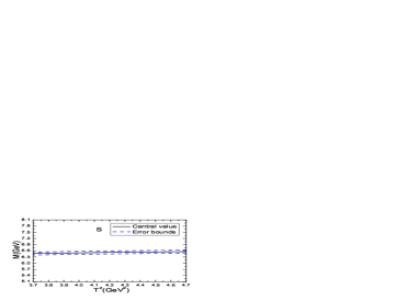
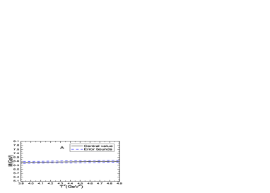
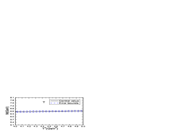
Now let us take into account all uncertainties of the input parameters, such as the continuum threshold parameter, the $c$-quark mass, the gluon condensate, the Borel parameter, and obtain the values of the masses and pole residues of the scalar, axialvector and tensor fully-charm tetraquark states, which are shown explicitly in Table 1 and Fig.1. From Fig.1, we can see that the predicted masses are rather stable with variations of the Borel parameters, the uncertainties originate from the Borel parameters are very small, it is reliable to extract the tetraquark masses.

The quantum field theory allows non-vanishing couplings between an interpolating current and a hadron (or several hadrons or a hadron system or several hadron systems) provided they have the same quantum numbers. On the other hand, a hadron has many Fock states, a Fock state couples potentially to an interpolating current with the same quantum numbers. In the present case, we can introduce the mixing angle $\theta$ and study the fully-charm tetraquark states with the currents $AA\cos\theta+\tilde{A}\tilde{A}\sin\theta$, where the $AA$ and $\tilde{A}\tilde{A}$ denote the $AA$-type and $\tilde{A}\tilde{A}$-type tetraquark currents respectively. We expect to obtain better QCD sum rules via fine-turning the parameter $\theta$ as the fully-charm tetraquark states have more than one Fock states.

$J^{PC}$ $T^{2}(\rm{GeV}^{2})$ $\sqrt{s_{0}}(\rm{GeV})$ pole $M_{X/Y}(\rm{GeV})$ $\lambda_{X/Y}(10^{-1}\rm{GeV}^{5})$
$0^{++}$ $3.9-4.5$ $7.05\pm 0.10$ $(39-63)\%$ $6.52\pm 0.10$ $6.17\pm 1.34$
$1^{+-}$ $4.1-4.7$ $7.10\pm 0.10$ $(38-62)\%$ $6.57\pm 0.10$ $5.17\pm 1.08$
$2^{++}$ $4.2-4.8$ $7.15\pm 0.10$ $(39-62)\%$ $6.60\pm 0.10$ $7.95\pm 1.63$
Table 1: The Borel parameters, continuum threshold parameters, pole contributions, masses and pole residues of the fully-charm tetraquark states.
$J^{PC}$ 1S 2S 3S $\overline{1\rm S}$ $\overline{2\rm S}$
$0^{++}(\tilde{A}\tilde{A})$ $6.52\pm 0.10$ $0.33\pm 0.10$
$0^{++}(AA)$ $5.99\pm 0.08$ $6.48\pm 0.08$ $6.94\pm 0.08$ $-0.20\pm 0.08$ $0.29\pm 0.08$
$1^{+-}(\tilde{A}\tilde{A})$ $6.57\pm 0.10$ $0.38\pm 0.10$
$1^{+-}(AA)$ $6.05\pm 0.08$ $6.52\pm 0.08$ $6.96\pm 0.08$ $-0.14\pm 0.08$ $0.33\pm 0.08$
$2^{++}(\tilde{A}\tilde{A})$ $6.60\pm 0.10$ $0.41\pm 0.10$
$2^{++}(AA)$ $6.09\pm 0.08$ $6.56\pm 0.08$ $7.00\pm 0.08$ $-0.10\pm 0.08$ $0.37\pm 0.08$
Table 2: The predicted fully-charm tetraquark masses from the QCD sum rules, where the $AA$-type tetraquark masses are taken from Refs.[4, 11], the overline on the 1S and 2S denotes that the $J/\psi J/\psi$ threshold is subtracted.
Refer to caption
Refer to caption
Refer to caption
Figure 1: The masses of the fully-charm tetraquark states with variations of the Borel parameters $T^{2}$, where the $S$, $A$ and $T$ denote the scalar, axialvector and tensor tetraquark states, respectively.

In Table 2, we also present the masses of the ground states and the first radial excited states of the $AA$ type tetraquark states from the QCD sum rules [4, 11], and the masses of the second radial excited states of the $AA$ type tetraquark states from the Regge trajectories [11]. From the Table, we can see that the 1S $\tilde{A}\tilde{A}$ type tetraquark states and the 2S $AA$-type tetraquark states have almost degenerated masses, they lie about $0.35\pm 0.09\,\rm{GeV}$ above the $J/\psi J/\psi$ threshold, the broad structure above the $J/\psi J/\psi$ threshold observed by the LHCb collaboration maybe consist of several diquark-antidiquark type $cc\bar{c}\bar{c}$ tetraquark states, more precise measurements are still needed, while the narrow structure $X(6900)$ can be assigned to be the second radial excited state of the scalar or axialvector $cc\bar{c}\bar{c}$ tetraquark state [11].

In the present work, we introduce the explicit P-wave to construct the diquark operators therefore the tetraquark operators. Without introducing the explicit P-waves, we can take the diquark operators $Q^{T}_{j}CQ_{k}$, $Q^{T}_{j}C\gamma_{5}Q_{k}$ and $Q^{T}_{j}C\gamma_{\mu}\gamma_{5}Q_{k}$ in the symmetric color sextet and the diquark operators $Q^{T}_{j}C\gamma_{\mu}Q_{k}$, $Q^{T}_{j}C\sigma_{\mu\nu}Q_{k}$, $Q^{T}_{j}C\sigma_{\mu\nu}\gamma_{5}Q_{k}$ in the antisymmetric color antitriplet, which satisfy the Fermi-Dirac statistics, as the basic constituents to construct the fully-heavy tetraquark states with the same flavor. In Ref.[4], we choose the diquark operators $\varepsilon^{ijk}Q^{T}_{j}C\gamma_{\mu}Q_{k}$ as the basic constituents to study the ground state masses of the $J^{PC}=0^{++}$, $1^{+-}$ and $2^{++}$ fully heavy tetraquark states, and obtain the lowest mass $6.0\,\rm{GeV}$ for the $cc\bar{c}\bar{c}$ tetraquark states. In Ref.[11], we study the masses of the first radial excited states of the $cc\bar{c}\bar{c}$ tetraquark states with the QCD sum rules and obtain masses of the second radial excited states with the Regge trajectories, the predicted masses of the first radial excited states and the second radial excited states are about $6.5\,\rm{GeV}$ and $6.9\,\rm{GeV}$, respectively, see Table 2. In Ref.[6], W. Chen et al take both the diquark operators in the color sextet and color antitriplet as the basic constituents to study the mass spectrum of the fully heavy tetraquark states with the moments QCD sum rules, and obtain the tetraquark masses about $6.3\sim 6.9\,\rm{GeV}$, where the lowest mass of the scalar $cc\bar{c}\bar{c}$ tetraquark states is about $6.4\,\rm{GeV}$. In Ref.[13], J. R. Zhang takes $c^{T}_{j}Cc_{k}$, $c^{T}_{j}C\gamma_{5}c_{k}$ and $c^{T}_{j}C\gamma_{\mu}\gamma_{5}c_{k}$ in the color sextet and the diquark operator $c^{T}_{j}C\gamma_{\mu}c_{k}$ in the color antitriplet to study the $J^{P}=0^{+}$ fully-charm tetraquark states with the QCD sum rules, and obtain almost degenerated masses, about $6.5\,\rm{GeV}$. Those different predictions in Refs.[4, 6, 11, 13] maybe originate from the different input parameters and different Borel windows. They are all compatible with the experimental data from the LHCb collaboration within uncertainties at the present time [9], more experimental data are still needed to select the best QCD sum rules.

4 Conclusion

In this article, we introduce a relative P-wave to construct the doubly-charm axialvector diquark operator, then take the doubly-charm axialvector (anti)diquark operator as the basic constituent to construct the scalar and tensor tetraquark currents to study the scalar, axialvector and tensor fully-charm tetraquark states with the QCD sum rules. The numerical results indicate that the ground state $\tilde{A}\tilde{A}$ type tetraquark states and the first radial excited states of the $AA$ type tetraquark states have almost degenerated masses, they lie about $0.35\pm 0.09\,\rm{GeV}$ above the $J/\psi J/\psi$ threshold, the broad structure above the $J/\psi J/\psi$ threshold observed by the LHCb collaboration maybe consist of several diquark-antidiquark type fully-charm tetraquark states.

Acknowledgements

This work is supported by National Natural Science Foundation, Grant Number 11775079.

References

  • [1] S. K. Choi et al, Phys. Rev. Lett. 91 (2003) 262001.
  • [2] P. A. Zyla et al, Prog. Theor. Exp. Phys. 2020 (2020) 083C01.
  • [3] R. J. Lloyd and J. P. Vary, Phys. Rev. D70 (2004) 014009; N. Barnea, J. Vijande and A. Valcarce, Phys. Rev. D73 (2006) 054004; A. V. Berezhnoy, A. V. Luchinsky and A. A. Novoselov, Phys. Rev. D86 (2012) 034004; W. Heupel, G. Eichmann and C. S. Fischer, Phys. Lett. B718 (2012) 545; Y. Bai, S. Lu and J. Osborne, Phys. Lett. B798 (2019) 134930; J. M. Richard, A. Valcarce and J. Vijande, Phys. Rev. D95 (2017) 054019.
  • [4] Z. G. Wang, Eur. Phys. J. C77 (2017) 432; Z. G. Wang and Z. Y. Di, Acta Phys. Polon. B50 (2019) 1335.
  • [5] M. Karliner, J. L. Rosner and S. Nussinov, Phys. Rev. D95 (2017) 034011; M. N. Anwar, J. Ferretti, F. K. Guo, E. Santopinto and B. S. Zou, Eur. Phys. J. C78 (2018) 647; A. Esposito and A. D. Polosa, Eur. Phys. J. C78 (2018) 782; J. Wu, Y. R. Liu, K. Chen, X. Liu and S. L. Zhu, Phys. Rev. D97 (2018) 094015.
  • [6] W. Chen, H. X. Chen, X. Liu, T. G. Steele and S. L. Zhu, Phys. Lett. B773 (2017) 247.
  • [7] C. Hughes, E. Eichten and C. T. H. Davies, Phys. Rev. D97 (2018) 054505.
  • [8] V. R. Debastiani and F. S. Navarra, Chin. Phys. C43 (2019) 013105; M. S. Liu, Q. F. Lu, X. H. Zhong and Q. Zhao, Phys. Rev. D100 (2019) 016006; X. Chen, arXiv:2001.06755; M. A. Bedolla, J. Ferretti, C. D. Roberts and E. Santopinto, arXiv:1911.00960; C. Deng, H. Chen and J. Ping, arXiv:2003.05154; P. Lundhammar and T. Ohlsson, arXiv:2006.09393.
  • [9] R. Aaij et al, arXiv:2006.16957.
  • [10] M. S. liu, F. X. Liu, X. H. Zhong and Q. Zhao, arXiv:2006.11952; Q. F. Lu, D. Y. Chen and Y. B. Dong, arXiv:2006.14445; H. X. Chen, W. Chen, X. Liu and S. L. Zhu, arXiv:2006.16027; X. Y. Wang, Q. Y. Lin, H. Xu, Y. P. Xie, Y. Huang and X. Chen, arXiv:2007.09697; J. F. Giron and R. F. Lebed, arXiv:2008.01631; L. Maiani, arXiv:2008.01637; K. T. Chao and S. L. Zhu, arXiv:2008.0767.
  • [11] Z. G. Wang, Chin. Phys. C44 (2020) 113106.
  • [12] G. Yang, J. Ping, L. He and Q. Wang, arXiv:2006.13756; R. Maciula, W. Schafer and A. Szczurek, arXiv:2009.02100; R. M. Albuquerque, S. Narison , A. Rabemananjara, D. Rabetiarivony and G. Randriamanatrika, arXiv:2008.01569; J. Sonnenschein and D. Weissman, arXiv:2008.01095.
  • [13] J. R. Zhang, arXiv:2010.07719.
  • [14] Z. G. Wang, Eur. Phys. J. C71 (2011) 1524; R. T. Kleiv, T. G. Steele and A. Zhang, Phys. Rev. D87 (2013) 125018.
  • [15] Z. G. Wang, Commun. Theor. Phys. 59 (2013) 451.
  • [16] M. A. Shifman, A. I. Vainshtein and V. I. Zakharov, Nucl. Phys. B147 (1979) 385; Nucl. Phys. B147 (1979) 448.
  • [17] L. J. Reinders, H. Rubinstein and S. Yazaki, Phys. Rept. 127 (1985) 1.
  • [18] Z. G. Wang, Int. J. Mod. Phys. A35 (2020) 2050138.
  • [19] Z. G. Wang and Z. Y. Di, Eur. Phys. J. C79 (2019) 72; Z. G. Wang, Eur. Phys. J. C79 (2019) 184; Z. G. Wang, Acta Phys. Polon. B51 (2020) 435.
  • [20] Z. G. Wang, Phys. Rev. D101 (2020) 074011.
  • [21] Z. G. Wang, Phys. Rev. D102 (2020) 014018.
  • [22] P. Colangelo and A. Khodjamirian, hep-ph/0010175.
  • [23] L. Maiani, F. Piccinini, A. D. Polosa and V. Riquer, Phys. Rev. D89 (2014) 114010; M. Nielsen and F. S. Navarra, Mod. Phys. Lett. A29 (2014) 1430005; Z. G. Wang, Commun. Theor. Phys. 63 (2015) 325.
  • [24] R. F. Lebed and A. D. Polosa, Phys. Rev. D93 (2016) 094024.
  • [25] Z. G. Wang, Eur. Phys. J. C77 (2017) 78; Z. G. Wang, Eur. Phys. J. A53 (2017) 19.
  • [26] H. X. Chen and W. Chen, Phys. Rev. D99 (2019) 074022; Z. G. Wang, Chin. Phys. C44 (2020) 063105.