Disentangling Neural Architectures and Weights:
A Case Study in Supervised Classification

Abstract

The history of deep learning has shown that human-designed problem-specific networks can greatly improve the classification performance of general neural models. In most practical cases, however, choosing the optimal architecture for a given task remains a challenging problem. Recent architecture-search methods are able to automatically build neural models with strong performance but fail to fully appreciate the interaction between neural architecture and weights.

This work investigates the problem of disentangling the role of the neural structure and its edge weights, by showing that well-trained architectures may not need any link-specific fine-tuning of the weights. We compare the performance of such weight-free networks (in our case these are binary networks with {0, 1}-valued weights) with random, weight-agnostic, pruned and standard fully connected networks. To find the optimal weight-agnostic network, we use a novel and computationally efficient method that translates the hard architecture-search problem into a feasible optimization problem. More specifically, we look at the optimal task-specific architectures as the optimal configuration of binary networks with {0, 1}-valued weights, which can be found through an approximate gradient descent strategy. Theoretical convergence guarantees of the proposed algorithm are obtained by bounding the error in the gradient approximation and its practical performance is evaluated on two real-world data sets. For measuring the structural similarities between different architectures, we use a novel spectral approach that allows us to underline the intrinsic differences between real-valued networks and weight-free architectures.

1 Introduction

The exceptionally good performance of neural-based models can be considered the main responsible for the recent huge success of AI. To obtain the impressive learning and predictive power of nowadays models, computer scientists have spent years designing, fine-tuning and trying different and increasingly sophisticated network architectures. In particular, it has become clear that the optimal edge structure greatly depends on the specific task to be solved, e.g. CNNs for image classification szegedy2017inception ; wei2015hcp , RNNs for sequence labeling ma2016end ; graves2012supervised and Transformers for language modeling vaswani2017attention ; devlin2019bert . But this has been a pretty painful path as designing new neural architectures often requires considerable human effort and testing them is a challenging computational task.

Existing methods for a fully-automated architecture search are mostly based on two strategies: (i) architecture search schemes zoph2016neural ; liu2018darts ; gaier2019weight ; you2020greedynas , which look for optimal neural structures in a given search space , and (ii) weight pruning procedures Han2015LearningBW ; Frankle2019TheLT ; Zhou2019DeconstructingLT , which attempt to improve the performance of large (over-parameterized) networks by removing the ‘less important’ connections. Neural models obtained through these methods have obtained good results on benchmark data sets for image classification (e.g. CIFAR-10) or language modeling (e.g. Penn Treebank) yu2019playing . What remains unclear is whether such networks perform well because of their edge structures, their optimized weight values or a combination of the two. A puzzling example can be found in the framework of weight-agnostic neural networks gaier2019weight , where models are trained and tested by enforcing all connections to share the same weight value. Their decent classification power suggests that the contribution of fine-tuned weights is limited gaier2019weight but the conclusion should probably be revised as recent studies zhang2020deeper show that the output can actually be very sensitive to the specific value of the shared weight.

In this work, we try to disentangle the role of neural architecture and weight values by considering a class of weight-free neural models which do not need any tuning or random-sampling of the connections weight(s). To train such models in a weight-free fashion, we define a new algorithm that optimizes their edge structure directly, i.e. without averaging over randomly-sampled weights, as for weight-agnostic networks gaier2019weight , or training edge-specific real-value weights, as in other architecture search methods liu2018darts ; Frankle2019TheLT . The proposed scheme is obtained by formulating the architecture search problem as an optimization task over the space of all possible binary networks with {0, 1}-valued weights. Given a fully connected neural model with connections ${\cal C}=\{i\}_{i=1}^{d}$, for example, the search space is the power set ${\mathcal{P}}({\cal C})$ and the goal is to find a subset of nonzero connections ${\cal C}_{*}\subset{\cal C}$ that minimizes a given objective function. In practice, formulating architecture search as a discrete optimization problem is advantageous because i) the neural architecture associated with the optimal binary-weight optimal assignment, ${\cal C}^{*}\subset{\cal C}$, does not depend on specific weight values and ii) the discrete optimization problems can be approximated arbitrarily well by continuous optimization problems.

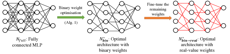
Figure 1: We first obtain the optimal neural architecture $N^{*}_{\textbf{bin}}$ by performing binary weight optimization on the base network $N_{\mbox{full}}$, and then fine tune real-value weights on top of $N^{*}_{\textbf{bin}}$ to obtain $N^{*}_{\textbf{bin}\to\textbf{real}}$. The performance gap between $N^{*}_{\textbf{bin}}$ and $N^{*}_{\textbf{bin}\to\textbf{real}}$ is the contribution of the weight values.

To analyze the intrinsic predictive power of weight-free networks, we compare their performance with a real-valued version of them, where fine-tuned weights are attached to all non-vanishing connections, i.e. a real-valued network with weights $\{w_{i}>0\}_{i\in{\cal C_{*}}}$. Figure 1 illustrates the major steps of our strategy. Finally, we summarize the structural differences of the obtained networks, by looking at the spectrum of their Laplacian matrix. Graph spectral analysis has been used in computational biology for comparing the structure of physical neural networks, e.g. the brain connectome de2014laplacian ; villegas2014frustrated ; 4390947 , but, to the best of our knowledge, rarely exploited to evaluate or classify artificial neural models in an AI or machine learning framework.

The contributions of this work are the following:

• We formulate the architecture search task as a binary optimization problem and propose a computationally efficient algorithm.

• We provide theoretical convergence guarantees for the proposed method. To the best of our knowledge, this is the first time convergence guarantees have been provided for an architecture-search method.

• We quantitatively measure the contribution of neural architectures and weight by comparing the performance of weight-free and real-valued networks on image and text classification tasks. Results suggest that binary networks trained through the proposed algorithm often outperform both binary networks obtained through other techniques and real-valued ones (probably because they are less prone to training data over-fitting).

• We propose a novel and bilogically-inspired method to measure the similarity between neural architectures based on the eigen-spectrum of their Laplacian matrix de2014laplacian .

2 Related Work

Neural architecture-search methods construct a neural architecture incrementally, by augmenting a connection or an operation at each step. Early methods stanley2002evolving ; zoph2016neural ; real2019regularized employ expensive genetic algorithms or reinforcement learning (RL). More recent schemes either design differentiable losses liu2018darts ; xie2019snas , or use random weights to evaluate the performance of the architecture on a validation set gaier2019weight ; pham2018efficient . Unlike these methods, that search architectures by adding new components, our method removes redundant connections from an over-parameterized ‘starting’ network, e.g. a fully-connected multi-layer perceptron (MLP). Network pruning approaches start from pre-trained neural models and prune the unimportant connections to reduce the model size and achieve better performance han2015deep ; collins2014memory ; Han2015LearningBW ; Frankle2019TheLT ; yu2019playing . These methods prune existing task-specific network architectures e.g. CNNs for image classification, whereas our method starts from generic architectures (that would perform poorly without pruning), e.g. fully-connected MLPs. In addition, our method does not require any pre-training. Network quantization and binarization reduces the computational cost of neural models by using lower-precision weights jacob2018quantization ; zhou2016dorefa , or mapping and hashing similar weights to the same value chen2015compressing ; hu2018hashing . In an extreme case, the weights, and sometimes even the inputs, are binarized, with positive/negative weights mapped to $\pm 1$ soudry2014expectation ; courbariaux2016binarized ; hubara2017quantized ; shen2019searching ; courbariaux2015binaryconnect . As a result, these methods keep all original connections, i.e. do not perform any architecture search.

3 Background

Supervised learning of real-valued models

Let $\mathcal{D}=\{z_{i}=(x_{i},y_{i})\in{\cal X}\times{\cal Y}\}_{i=1}^{n}$ be a training set of vectorized objects, $x_{i}$, and labels, $y_{i}$. Let $f:{\cal W}\times{\cal X}\times{\cal Y}\to\mathbf{R}$, where ${\cal W}$ is a given parameter space, be such that $f(w,z)$ yields the miss-classification value associated with object-label pair $z\in{\cal D}$. Furthermore, let $f$ be of the form $f(w,z)=\ell(\psi(w,z),y)$, where $\ell:{\cal Y}\times{\cal Y}\to{\mathbf{R}}$ is a fixed cost function and $\psi:{\cal W}\times{\cal X}\to{\cal Y}$ the classification model. For any fixed choice of parameter $w\in{\cal W}$, $\psi(w,z)$ maps vectorized objects $x\in{\cal X}$ into labels $y\in{\cal Y}$. Classifiers such as $\psi$ can be trained by minimizing the average loss

$$F(w)=|\mathcal{D}|^{-1}\sum_{z\in{\cal D}}f(w,z).$$ (1)

In standard neural training ${\cal W}={\mathbf{R}}^{d}$ and $w_{*}=\arg\min_{w\in{\cal W}}F(w)$ is usually found through Stochastic Gradient Descent (SGD) updates

$$w^{t}\leftarrow w^{t-1}-\frac{\eta^{t}}{|\mathcal{Z}^{t}|}\sum_{z\in\mathcal{Z}^{t}}\frac{\partial f(z;w^{t-1})}{\partial w^{t-1}},$$ (2)

where $\eta^{t}>0$ is the learning rate and $\mathcal{Z}^{t}\subseteq\mathcal{D}$ a randomly selected mini-batch at step $t$.

Training binary networks

Unlike conventional neural models, where ${\cal W}={\mathbf{R}}^{d}$, a binary-weight neural model is a function $\psi:{\cal W}\times{\cal X}\to{\cal Y}$, where ${\cal W}=\{a,b\}^{d}$, with $a,b\in{\mathbf{R}}$ being fixed values. Here we focus on a special class of binary models where $a=0$ and $b=1$ but other choices are possible, e.g. a popular setting is $a=-1$ and $b=1$.

Similarly to the case ${\cal W}={\mathbf{R}}^{d}$, the single-input miss-classification value is $f:\{0,1\}^{d}\times{\cal X}\times{\cal Y}\to{\mathbf{R}}$ and $\psi$ can be trained by setting $W=\{0,1\}^{d}$ (1). Minimizing (1) over $\{0,1\}^{d}$, however, is a challenging discrete optimization problem, with the size of the search space, ${\mathbf{P}}(\{i\}_{i=1}^{d})$, increasing exponentially with the growth of $d$.

SGD for binary optimization

One possible way to minimize (1) over ${\cal W}=\{0,1\}^{d}$ is to i) define a suitable continuous approximation of the minimization problem $\min_{w\in\{0,1\}^{d}}F(w)$, ii) solve such a continuous approximation through standard SGD updates and iii) binarize the obtained solution at the end. The strategy proposed here is to consider an approximate binary-weight constraints, $\{0,1\}\to[0,1]$ and minimize (1) over ${\cal V}=[0,1]^{d}$ under the further (but more handable) constraint $v=B_{M}(w)$, where $B_{M}:{\mathbf{R}}^{d}\to{\cal V}$, $w\in{\mathbf{R}}^{d}$ is an approximate binarization function and $M>0$ a parameter controlling the ‘sharpness’ of the approximation. More explicitly, we propose to train $\psi$ by solving

$$\begin{array}[]{ll}\text{minimize}&F(B_{M}(w))\\ \text{s.t.}&w\in{\mathbf{R}}^{d}\end{array}\quad\Leftrightarrow\quad\begin{array}[]{ll}\text{minimize}&F(v)\\ \text{s.t.}&v=B_{M}(w)\text{ and }w\in{\mathbf{R}}^{d}\end{array}$$ (7)

where $F$ is given in (1) and $B_{M}:{\mathbf{R}}^{d}\to[0,1]^{d}$ is the approximate step function

$$B_{M}(w)=\sigma(Mw)=(1+\exp(-M\cdot w))^{-1}$$

As $B_{M}$ is differentiable for all $M<\infty$, we can solve (7) through SGD updates

$$w^{t} \leftarrow w^{t-1}-\frac{\eta^{t}}{|\mathcal{Z}^{t}|}\sum_{z\in\mathcal{Z}^{t}}\nabla f(v^{t-1},z)\circ\sigma_{M}^{\prime}(w),$$ (8)

where $[\nabla f(v,z)]_{i}=\frac{\partial f(v,z)}{\partial v_{i}}$, ‘$\circ$’ denotes element-wise vector multiplication and $\sigma_{M}^{\prime}(w)=\sigma_{M}(w)\circ(1-\sigma_{M}(w))=B_{M}(w)\circ(1-B_{M}(w))$ is the first derivative of $B_{M}(w)$.

4 Method

A major difficulty of solving (7) is that, as $M$ in $B_{M}$ increases, the approximation quality improves but gradient-based updates may become exponentially small. Figure 2 shows the shape of $B_{M}(w)$ and its first derivative, $B_{M}^{\prime}(w)=\nabla B_{M}(w)=B_{M}(w)\circ(1-B_{M}(w))$, for different values of $M$. In particular, note that $B_{M}^{\prime}(w)\approx 0$ in large parts of its domain, even for reasonably small values of $M$. Inspired by the BinaryConnect approach courbariaux2015binaryconnect , we define two binarization functions (by setting $M$ to two different values): i) $B_{M_{hard}}$ with $M_{hard}>>1$ , to be used at forward-propagation time, and ii) $B_{M_{soft}}$, with $M_{soft}<M_{hard}$, to compute the gradient updates. The idea is to solve (7) with $M=M_{hard}$, which is a good approximation of the original discrete optimization problem, through the relaxed SGD weight updates:

$$w^{t}\leftarrow w^{t-1}-\frac{\eta^{t}}{|\mathcal{Z}^{t}|}\sum_{z\in\mathcal{Z}^{t}}\nabla f(B_{M_{hard}}(w^{t-1}),z)\circ B_{M_{soft}}^{\prime}(w^{t-1})$$ (9)

Algorithm 1 is a pseudo-code implementation of this idea.

Algorithm 1 SGD-based architecture search (one epoch)

Inputs:
   Randomly initialized neural model with real-valued weights, $w^{0}\in\mathbf{R}^{d}$, training data set, $\{z_{i},\cdots,z_{n}\}$, learning rates, $\{\eta^{1},\cdots,\eta^{T}\}$, binarization function, $B_{M}$, soft- and hard-binarization constants, $M_{hard}>>1$ and $M_{soft}<M_{hard}$

Binary optimization by SGD:

  for $t=1,\cdots,T$ do

     Obtain mini-batch: $\mathcal{Z}=\{z_{i},\cdots,z_{i+k-1}\}$

     Compute hard-binarized weights: $v=B_{M_{hard}}(w^{t-1})$

     Compute loss: $F(v)=k^{-1}\sum_{z\in\mathcal{Z}}f(v,z)$

     Update unconstrained weights: $w^{t}\leftarrow w^{t-1}-\eta^{t}k^{-1}\sum_{z\in\mathcal{Z}}\nabla f(v,z)\circ B_{M_{soft}}^{\prime}(w^{t-1})$

  end for

Extract architecture:

  Obtain binary network $\psi_{bin}=\lim_{M\to\infty}\psi(B_{M}(w^{T}),z)$

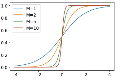
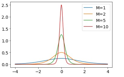
Figure 2: Shape of the parameterized binarization function $B_{M}$ (upper) and its derivative (bottom) with different values of $M$ .

Remarks

The hard-binarization parameter, $M_{hard}$, which defines the optimization problem to be solved, should be fixed a priori (we set $M_{hard}=50$ in the experiments of Section 5). The soft-binarization parameter, $M_{soft}$, which defined the slackness of the gradient approximations, could in principle be tuned through standard cross-validation procedures, but we keep it fixed in this work ($M_{soft}=M_{hard}/10$ in Section 5). Figure 2 shows the quality of the continuous approximation for different values of $M_{hard}$. Large values of $M_{hard}$ make the optimization task harder but reduce the error made in converting the approximately-binary trained network, $\psi(B_{M_{hard}}(w_{*}),z)$ with $B_{M_{hard}}(w_{*})\in[0,1]$ and $w_{*}=w^{T}$ in Algorithm 1, to the ‘true’ binary network $\psi_{bin}(w,z)=\lim_{M\to\infty}\psi(B_{M}(w_{*}),z)$ (see last line of Algorithm 1). Figure 3 shows the convergence of Algorithm 1 for different choices of $M_{hard}$ and $M_{soft}$. Note that choosing $M_{soft}<<M_{hard}$ may be counterproductive when $M_{hard}$ is small but consistently helps the SGD updates converge when $M_{hard}>>1$.

Algorithm convergence

In the remaining of this section, we consider single-input mini-batch, i.e. we set ${\cal Z}^{t}=\{\tilde{z}\}$ for all $t=1,\dots,T$ and prove that the Algorithm 1 converges to a local optimum of (7). As a consequence, we can state that Algorithm 1 can be consistently used to solve arbitrarily good approximations of the unfeasible discrete optimization problem “$\min_{w\in\{0,1\}^{d}}F(w)$” with $F$ given in (1). We show that the approximate gradient updates (9) are close-enough to the gradient updates needed for solving (7), i.e. the sharp ($M=M_{hard}$) approximation of the original discrete problem.

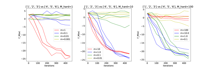
Figure 3: Convergence of Algorithm 1 for varying values of $M_{hard}$ and $M_{soft}$. The learning task is to distinguish between two groups of hand-written digits, $\{1,2,3\}$ and $\{4,5,6\}$. We use a constant learning parameter and 100 images of each class as training set (see Section 5 for detailed experimental setup). Solid and dashed lines correspond to the median and the 25th/75th percentiles over 10 independent runs.

We first assume that the loss function $f$ is differentiable over ${\cal V}=[0,1]^{d}$ and

$$\max_{v\in{\cal V},z\in{\cal X}\times{\cal Y}}\|\nabla f(v,z)\|^{2}\leq G^{2},\quad\mbox{and}\quad f(v,z)-f(v^{\prime},z)\geq\nabla f(v^{\prime},z)^{T}(v-v^{\prime})$$ (10)

and prove the following lemma.

Lemma 4.1.

Assume that $f$ meets the requirements in (10), then $F(v):[0,1]^{d}\to{\mathbf{R}}$ defined as $F(v)=|{\cal D}|^{-1}\sum_{z\in{\cal D}}f(v,z)$ is also a convex function, i.e. $F(v)-F(v^{\prime})\geq\nabla F(v^{\prime})^{T}(v-v^{\prime})$

Remarks

The convergence of the stochastic gradient descent does not follow automatically from the assumption on $f$ and Lemma 4.1 for two reasons: i) $F(v)=|{\cal D}|^{-1}\sum_{z\in{\cal D}}f(v,z)$ is component-wise composed with the non-convex function $B_{M_{hard}}(w)$ and ii) we use an approximation of the ‘true’ gradient of $F(B_{M_{hard}}(w))$.

To show that the approximated updates (9) can be used to solve (7) we need the following lemma.

Lemma 4.2.

For any $w^{t}$, $t=0,\dots,T$, and $\tilde{z}\in{\cal D}$, the gradient updates (9) are equivalent to

$$v^{t+1} \leftarrow v^{t}-\eta_{t}(\nabla f(v^{t},\tilde{z})+r^{t}),$$ (11)

where $v^{t}=B_{M_{hard}}(w^{t})$,

$$r^{t} =\nabla f(v^{t},\tilde{z})-B_{M_{hard}}^{\prime}(\xi^{t})\circ\nabla f(v^{t},\tilde{z})\circ B_{M_{soft}}^{\prime}(w^{t}),$$ (12)

with $\xi^{t}\in[w^{t},w^{t}-\eta_{t}\nabla f(v^{t},\tilde{z})\circ B_{M_{soft}}(w^{t})]$. Furthermore, the error terms, $r^{t}$, $t=1,\dots,T$, obey

$$\|r^{t}\|^{2}\leq G^{2}C^{2}\quad C=1+\frac{M_{hard}M_{soft}}{16}$$ (13)

with $G$ defined in (10).

Remark

Lemma 4.2 is essentially a consequence of the Mean Value Theorem. The proof starts by applying $B_{M_{hard}}$ to both sides of (9) and then uses $f(a+b)=f(a)+\nabla f(c)^{T}b$, $c\in[a,a+b]$ to isolate the first term in the right-hand side of (12).

Finally, based on the lemmas above and an additional assumption that $\eta_{t}=\frac{c}{t}$ for all $t=1,\dots,T$, $c\in\mathbf{R}_{+}$, we obtain the following theorem, which proves that the approximate updates (11) converge to $w_{*}=\text{arg }\min_{w\in{\mathbf{R}}}F(B_{M_{hard}}(w))$.

Theorem 4.3.

Assume that the cost function $f:[0,1]^{d}\to{\mathbf{R}}$ meet the requirements in (10), and let $F(w)=|{\cal D}|^{-1}\sum_{z\in{\cal D}}f(B_{M_{hard}}(w),z)$, $w^{T}$ be the output of Algorithm 1, $w^{*}=\text{arg }\min_{w\in{\mathbf{R}}^{d}}F(B_{M_{hard}}(w))$, then

$$\mathbf{E}\left(F(B_{M_{hard}}(w^{T}))-F(B_{M_{hard}}(w^{*}))\right)\leq G^{2}\frac{c\left(1+C^{2}\right)}{2}\frac{1+\log T}{T},$$ (14)

where $\mathbf{E}(\cdot)$ is the expectation over the random sampling of $\tilde{z}\in{\cal D}$ and $C$ is the constant defined in Lemma 4.2.

5 Experiments

Data sets

We run a series of similar training-testing experiments on two real-world data sets, ${\cal D}\in\{{\cal D}_{mnist},{\cal D}_{citeseer}\}$. The first is a collection of vectorized images of hand-written digits from the MNIST database and the second a collection of vectorized abstracts of scientific papers from the Citeseer database. Both data sets consist of labeled objects that we represent through $(I=64)$-dimensional, real-valued, unit norm vectors, i.e. $|x|=64$ and $x^{T}x=1$ for all $x\in{\cal D}_{u}$, $u\in\{mnist,citeseer\}$. The original MNIST images are resized (by cropping 2 pixels per side and pooling over 64 non-overlapping windows), vectorized and normalized. The original bag-of-words, 3703-dimensional, integer-valued embedding vectors of the Citeseer abstracts are reduced to $I$ dimensions by projecting into the $d$-dimensional space spanned by the first $I$ Principal Components of the entire corpus.

Models

For all experiments, the architecture search-space boundaries are defined by

$$\psi(w,x)=\text{ReLU}\left(\sum_{i=1}^{I}\tanh\left(\sum_{j=1}^{I}[w_{2}]_{ij}\tanh\left(\sum_{k=1}^{I}[w_{1}]_{jk}x_{k}\right)\right)\right)$$ (15)

where $x\in{\cal X}={\mathbf{R}}^{I}$, $[w_{1},w_{2}]\in{\cal W}$, ${\cal W}=\{0,1\}^{d}$ for the binary networks and ${\cal W}={\mathbf{R}}_{+}^{d}$ for the real networks, $d=2I^{2}$, $\tanh(w)$ is the hyperbolic tangent activation function and $\text{ReLU}(w)=\log(1+e^{w})$. In all cases, the classifier $\psi$ in (15) is trained by minimizing

$$\quad F(w)=|{\cal D}|^{-1}\sum_{(x,y)\in{\cal D}}\psi(w,x)(1-2y)$$ (16)

over ${\cal W}\in\{\{0,1\}^{d},{\mathbf{R}}^{d}_{+}\}$. The nonnegativity constraint imposed on real-networks is not essential but we introduce it here to make the comparison between real- and $\{0,1\}$-valued networks fairer and conceptually easier. We compare five different training strategies:

• real and real$\to$bin: the real network is $\psi(w,x)$ with $w=\min_{w\in{\mathbf{R}}^{d}_{+}}F(w)$ and the binary network $\psi(w^{\prime},x)$ with

  $$w^{\prime}=B_{\infty}(w-\xi_{*}),\quad\xi_{*}=\text{arg }\min_{\xi\in T_{w}}F(B_{\infty}(w-\xi))$$ (17)

  where $T_{w}$ is the set of the $\{10,\cdots,100\}$th percentiles of all entries of $w$.

• lottery and lottery$\to$bin: the real network is $\psi(w,z)$ with

  $$w=\arg\min_{1\leq t\leq T}F(w^{t})$$

  where the elements of the sequence $w^{1},\dots,w^{T}$, $w^{t}\in{\mathbf{R}}_{+}^{d}$ are defined recursively by $w^{1}=\min_{w\in{\mathbf{R}}^{d}_{+}}F(w)$ and $w^{t}=w^{t-1}\circ w^{\prime}$, with $w^{\prime}$ obtained as in (17) with $w=w^{t-1}$, and the binary network is $\psi(w^{\prime},x)$ with $w^{\prime}=w\circ\tilde{w}$, with $\tilde{w}$ obtained as in (17) (see Frankle2019TheLT for more details about this procedure).

• bin and bin$\to$real: the binary network is $\psi(w^{\prime},z)$ with

  $$w^{\prime}=\min_{w\in\{0,1\}^{d}}F(w)$$

  obtained from Algorithm 1 and the real network is $\psi(w,z)$ where

  $$w=\text{arg }\min_{w\in{\mathbf{R}}_{+}^{d}}F(w\circ w^{\prime})$$

• random and random$\to$bin: the real network is $\psi(w,x)$ with $w=u^{2}$, $u\sim{\cal N}(0,1)^{d}$ and the binary network is $\psi(w^{\prime},x)$ with $w^{\prime}$ obtained as in (17).

• agnostic and agnostic$\to$real: the binary network is $\psi(w^{\prime},x)$ with

  $$w^{\prime}=\arg\min_{\bar{w}\in S}\left(\min_{\tilde{w}\in R_{\bar{w}}}F(\tilde{w})\right)$$

  where $\bar{w}\in S$ are random architectures $\bar{w}=B_{\infty}(w^{t}-\xi)$, $\xi\in T_{w}$ defined as in (17), $w^{t}=u^{2}$, $u\sim{\cal N}(0,1)^{d}$, $t=1,\dots,T$, and $\tilde{w}\in R_{\bar{w}}$ are shared-weight networks defined by $\tilde{w}=u_{0}\bar{w}$, $u_{0}\sim{\cal N}(0,1)$, and the real network is $\psi(w,x)$ with $w=u_{0}\bar{w}^{\prime}$, $u_{0}\sim{\cal N}(0,1)$.

Results

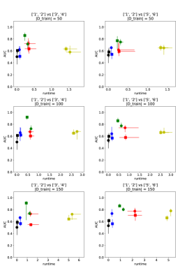
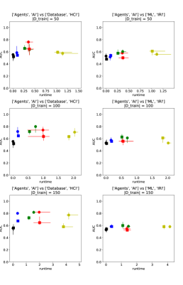
Figure 4: Runtime vs. AUC (over 50 test images) of the models trained to solve different tasks with training data sets of different sizes from the MNIST data set (columns 1 and 2) and the Citeseer data set (columns 3 and 4).

Figure 4 shows the performance of all methods listed above. For each data set, we train the models to distinguish between the two (non-overlapping) groups of classes reported by the plot titles. The scatter plots show the median and quantiles (error bars) of the run time over 10 independent experiments (x-axis) and AUC scores of the models (y-axis). For each task, we use a test set of 50 objects per class and three training sets of different sizes. The proposed model, bin or bin$\to$real (in green), achieves the best performance with comparable run time in all but one cases. In particular, it is striking to see that weight-free networks may so often outperform fine-tuned more flexible models. From an architecture-optimization perspective, the proposed method seems to produce better networks than both weight-agnostic search (agnostic, in yellow) and pruning (lottery ticket, in red) methods.

Laplacian spectra

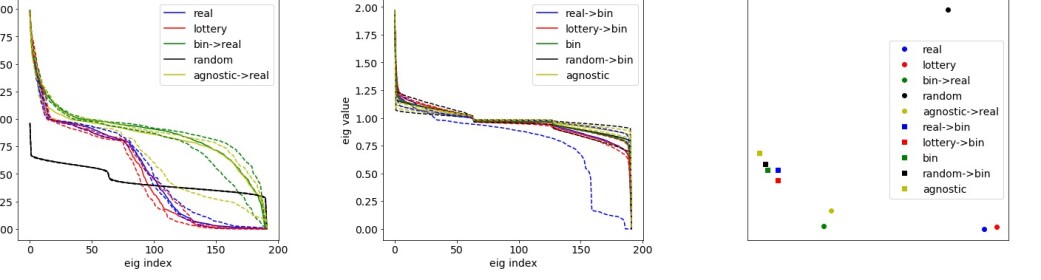
Figure 5: Citeseer data: spectrum of the network normalized Laplacian matrices (plots 1 and 2) and a 2-dimensional (PCA) representation of their distances.

Figure 5 shows the spectrum of the normalized Laplacian matrix of real and binary networks trained for discriminating images of digits 1 and 2 from the MNIST data set. Solid and dashed lines in the first two plots correspond to the median and quartiles of the eigenvalues (ordered by magnitude) obtained in 10 independent runs. The last plot is a 2-dimensional reduction (PCA) of the $3I$-dimensional vector space associated with the Laplacian spectra. Distances between different markers can be seen as a representation of the structural differences between models.

6 Discussions

The experiments show that weight-free networks found by our method can perform surprisingly well on different classification tasks and even outperform more flexible models. Real-valued fine-tuning of the edge structures may help when the classification task is hard but may also cause performance drop due to data overfitting. An analysis of the obtained networks based on their Laplacian spectra shows that different training strategies lead to highly different real-valued models but ‘spectrally similar’ architectures. An interesting question is whether such spectral similarities may be exploited in a transfer learning framework, and we leave this as future work.

Appendix A Definitions

Here is a summary of the notation used throughout this work:

$d\in{\mathbf{N}}$ maximum number of network connection

$M_{hard}>0$ hard-binarization constant

$0<M_{soft}\geq M_{hard}$ soft-binarization constant

${\cal X}$ input space

${\cal Y}$ label space

${\cal W}\in\{\{0,1\}^{d},[0,1]^{d},{\mathbf{R}}^{d}\}$ parameter space

$P_{Z}$ joint object-label distribution

$Z=(X,Y)\sim P_{Z}$, $X\in{\cal X}$ and $Y\in{\cal Y}$ object-label random variable

${\cal D}=\{z=(x,y)\text{ realization of }Z\sim P_{Z}\}$ training data set

$\psi:{\cal W}\times{\cal X}\to{\cal Y}$ classifier

$\ell:{\cal Y}\times{\cal Y}\to{\mathbf{R}}$ loss function

$f:{\cal W}\times{\cal X}\times{\cal Y}\to{\mathbf{R}}$ single-input classification error

$F:{\cal W}\to{\mathbf{R}}$, $F(w)=|{\cal D}|^{-1}\sum_{z\in{\cal D}}f(w,z)\approx{E}_{Z\sim P_{Z}}(f(w,Z))$ average classification error

$B_{M}:{\mathbf{R}}^{d}\to[0,1]^{d}$, $B_{M}(w)=\sigma_{M}(w)$ and $M>0$, binarization function

$B^{\prime}_{M}:{\mathbf{R}}^{d}\to[0,\frac{M}{4}]^{d}$, $B^{\prime}_{M}(w)=\sigma^{\prime}_{M}(w)$ and $M>0$, first derivative of the binarization function

$\sigma_{M}{\mathbf{R}}^{d}\to[0,1]^{d}$, $\sigma_{M}(w)=\frac{1}{1+e^{-Mw}}$ and $M>0$, sigmoid function

$\sigma^{\prime}_{M}:{\mathbf{R}}^{d}\to[0,\frac{M}{4}]^{d}$, $\sigma_{M}(w)=M\sigma_{M}(w)\circ(1-\sigma_{M}(w))$ and $M>0$, first derivative of the sigmoid function

$[\nabla g(w,z)]_{i}=\frac{\partial g(u,z)}{\partial u_{i}}|_{u=w}$ gradient of $g_{z}:{\cal W}\to{\mathbf{R}}$, $g_{z}(w)=g(w,z)$ at $(w,z)\in{\cal W}\times{\cal X}\times{\cal Y}$

$a\in[b,c]$, $a,b,c\in{\mathbf{R}}^{d}$ means $a_{i}\in[b_{i},c_{i}]$ for all $i=1,\dots,d$

$\text{diag}(a)\in{\mathbf{R}}^{d\times d}$ is such that $[\text{diag}(v)]_{ii}=v_{i}$ and $[\text{diag}(v)]_{ij}=0$ if $i\neq j$, $i,j=1,\dots,d$

Appendix B Assumptions and proofs

Assumption 1.

$f:[0,1]^{d}\to{\mathbf{R}}$, is differentiable over $[0,1]^{d}$ and obeys

$$\max_{v\in[0,1]^{d},z\in{\cal X}\times{\cal Y}}\|\nabla f(v,z)\|^{2} \leq G^{2},$$ (18)

$$\quad f(v,z)-f(v^{\prime},z) \geq\nabla f(v^{\prime},z)^{T}(v-v^{\prime}),$$ (19)

for all $v,v^{\prime}\in[0,1]^{d}$ and $z\in{\cal X}\times{\cal Y}$.

Lemma B.1.

Let $f:[0,1]^{d}\to{\mathbf{R}}$ satisfy Assumption 1, then $F(v):[0,1]^{d}\to{\mathbf{R}}$ aslo obeys

$$F(v)-F(v^{\prime})\geq\nabla F(v^{\prime})^{T}(v-v^{\prime}),$$ (20)

for all $v,v^{\prime}\in[0,1]^{d}$ and $z\in{\cal X}\times{\cal Y}$.

Proof of Lemma B.1

The convexity of $f$ implies the convexity of $F$ as

$$F(v)-F(v^{\prime}) =|{\cal D}|^{-1}\sum_{z\in{\cal D}}f(v,z)-f(v^{\prime},z)$$ (21)

$$\geq|{\cal D}|^{-1}\sum_{z\in{\cal D}}\nabla f(v^{\prime},z)^{T}(v-v^{\prime})$$ (22)

$$=\nabla F(v^{\prime})^{T}(v-v^{\prime}).$$ (23)

$\square$

Lemma B.2.

Let $\eta_{t}>0$ , $t=1,\dots,T$, and $w^{t}\in{\cal W}$ be defined by

$$w^{t+1}=w^{t}-\eta_{t}\nabla f(B_{M_{hard}}(w^{t}),z)\circ B^{\prime}_{M_{soft}}(w^{t}),\quad t=1,\dots,T,$$ (24)

and for any $z\in{\cal D}$. Then $v^{t}=B_{M_{hard}}(w^{t})$ obey

$$v^{t+1}=v^{t}-\eta_{t}(\nabla f(v^{t},z)+r^{t}),\quad t=1,\dots,T,$$ (25)

where

$$r^{t} =\nabla f(v^{t},z)-B_{M_{hard}}^{\prime}(\xi^{t})\circ\nabla f(v^{t},z)\circ B_{M_{soft}}^{\prime}(w^{t})$$ (26)

$$\xi^{t} \in[w^{t},w^{t}-\eta_{t}\nabla f(v^{t},z)\circ B_{M_{soft}}(w^{t})]$$ (27)

for all $z\in{\cal Z}$. Furthermore, the error terms, $r^{t}$, $t=1,\dots,T$, obey

$$\|r^{t}\|^{2}\leq G^{2}C^{2}\quad C=1+\frac{M_{hard}M_{soft}}{16}$$ (28)

with $G$ defined in (1).

Proof of LemmaB.2

Let $v=\sigma_{M}(w)$, for any $w\in{\mathbf{R}}^{d}$ and $M>0$. Then (24) is equivalent to (25) as

$$v^{t+1} =\sigma_{M_{hard}}\left(w^{t}-\eta_{t}\nabla f(\sigma_{M_{hard}}(w^{t}),z)\circ\sigma_{M_{soft}}^{\prime}(w^{t})\right)$$ (29)

$$=v^{t}-\eta_{t}\sigma_{M_{hard}}^{\prime}(\xi^{t})\circ\nabla f(\sigma_{M_{hard}}(w^{t}),z)\circ\sigma_{M_{soft}}^{\prime}(w^{t})$$ (30)

$$=v^{t}-\eta_{t}\nabla f(v^{t},z)+\eta_{t}r^{t}$$ (31)

$$r^{t} =\nabla f(v^{t},z)-\text{diag}\left(\sigma_{M_{hard}}^{\prime}(\xi^{t})\circ\sigma_{M_{soft}}^{\prime}(w^{t})\right)\cdot\nabla f(\sigma_{M_{hard}}(w^{t}),z)$$ (32)

$$=\nabla f(v^{t},z)-\text{diag}\left(\sigma_{M_{hard}}^{\prime}(\xi^{t})\circ\sigma_{M_{soft}}^{\prime}(w^{t})\right)\cdot\nabla f(v^{t},z)$$ (33)

$$\xi^{t} \in[w^{t},w^{t}-\nabla f(v^{t},z)\circ\sigma_{M_{soft}}^{\prime}(w^{t})]$$ (34)

where the first equality follows from the mean value theorem For any $w\in{\mathbf{R}}$ and $z\in{\cal Z}$, one has

$$\|r^{t}\|^{2} =\|\nabla f(v^{t},z)\|^{2}+\|\text{diag}\left(\sigma_{M_{hard}}^{\prime}(\xi^{t})\circ\sigma_{M_{soft}}^{\prime}(w^{t})\right)\cdot\nabla f(v^{t},z)\|^{2}$$ (35)

$$\quad-2\nabla f(v^{t},z)^{T}\text{diag}\left(\sigma_{M_{hard}}^{\prime}(\xi^{t})\circ\sigma_{M_{soft}}^{\prime}(w^{t})\right)\cdot\nabla f(v^{t},z)$$ (36)

$$\leq G^{2}+G^{2}\left(\frac{M_{soft}M_{hard}}{16}\right)^{2}+2G^{2}\frac{M_{soft}M_{hard}}{16}$$ (37)

$$=G^{2}\left(1+\frac{M_{soft}M_{hard}}{16}\right)^{2}$$ (38)

as, by definition, $G^{2}=\max_{(v,z)\in[0,1]^{d}\times{\cal x}\times{\cal Y}}\|\nabla f(v,z)\|^{2}$ and we have used $\max_{w\in{\mathbf{R}}^{d}}\sigma_{M}^{\prime}(w)=\frac{M}{4}$ for any $M>0$, the Cauchy-Schwarz inequality $v^{T}v^{\prime}\leq\|v\|\|v^{\prime}\|$ and $v^{T}\text{diag}(v^{\prime})\cdot v\leq\max_{i}v^{\prime}_{i}\|v\|^{2}$. $\square$

Theorem B.3.

Let $f:[0,1]^{d}\to{\mathbf{R}}$ satisfy Assumption (1), $\{w^{t}\in{\mathbf{R}}^{d}\}_{t=1}^{T}$ be the sequence of weights defined in (24), $\eta_{t}=\frac{c}{t}$, $t=1,\dots,T$, and $c>0$. Then

$${E}\left(F(B_{M_{hard}}(w^{T}))-F(B_{M_{hard}}(w^{*}))\right)\leq G^{2}\frac{c\left(1+C^{2}\right)}{2}\frac{1+\log T}{T},$$ (39)

where ${E}(w,z)$ is a short notation for ${E}_{Z\sim P_{Z}}(w,Z)$ and $G^{2}$ and $C$ are defined in Lemma B.2.

Proof of Theorem B.3

Assumption (1) and Lemma (B.1) imply that $F:[0,1]^{d}\to{\mathbf{R}}$ is a convex function over $[0,1]^{d}$. The first part of Lemma B.2 implies that the sequence of approximated ${\mathbf{R}}^{d}$-valued gradient updates (24) can be rewritten as the sequence of approximated $[0,1]^{d}$-valued gradient updates (25). The second part of Lemma B.2 implies that the norm of all error terms in (25) is bounded from above. In particular, as each $r^{t}$ is multiplied by the learning rate, $\eta_{t}$, it is possible to show that (25) converges to a local optimum of $F:[0,1]^{d}\to{\mathbf{R}}$. This implies that (24) converges to a local optimum of $F:{\mathbf{R}}^{d}\to{\mathbf{R}}$, since, by definition, the mapping $F(B_{hard}(w))$ is one-to-one and hence

$$v^{*} :=\text{arg }\min_{v\in[0,1]^{d}}F(v)$$ (40)

$$=B_{M_{hard}}\left(\text{arg}\min_{w\in{\mathbf{R}}^{d}}F(B_{M_{hard}}(w))\right)$$ (41)

$$=:B_{M_{hard}}(w_{*})$$ (42)

To show that (25) converges to a local optimum of $F:[0,1]^{d}\to{\mathbf{R}}$ we follows a standard technique for proving the convergence of stochastic and make the further (standard) assumption

$$E(r^{t})=0,\quad t=1,\dots,T.$$ (43)

First, we let $v^{t}$, $r^{t}$ and $\eta_{t}$, $t=1,\dots,T$, be defined as in Lemma B.2, and $z\in{\cal D}$ be the random sample at iteration $t+1$. Then

$$\|v^{t+1}-v^{*}\|^{2} =E\left(\|v^{t+1}-v^{*}\|^{2}\right)$$ (44)

$$=\|v^{t}-v^{*}\|^{2}-2\eta_{t}E(\nabla f(v^{t},\tilde{z})-r^{t})^{T}(v^{t}-v^{*})$$ (45)

$$\quad+\eta^{2}_{t}E\left(\|\nabla f(v^{t},\tilde{z})-r^{t}\|^{2}\right)$$

$$\leq\|v^{t}-v^{*}\|^{2}-2\eta_{t}E(\nabla f(v^{t},\tilde{z})^{T}(v^{t}-v^{*})+\eta^{2}_{t}\left(G^{2}+E(\|r^{t}\|^{2})\right)$$ (46)

$$\leq\|v^{t}-v^{*}\|^{2}+2\eta_{t}(F(v^{*})-F(v^{t}))+\eta^{2}_{t}G^{2}(1+C^{2})$$ (47)

where $G^{2}$ and $C$ are defined in (1) and (35). Rearranging terms one obtains

$$F(v^{t})-F(v^{*}) =\frac{\|v^{t}-v^{*}\|^{2}-\|v^{t+1}-v^{*}\|^{2}}{2\eta_{t}}+\frac{\eta_{t}}{2}G^{2}(1+C^{2})$$ (48)

and hence

$$E\left(F(v^{T})-F(v^{*})\right) =E\left(\frac{1}{T}\sum_{t=1}^{T}\left(F(v^{t})-F(v^{*})\right)\right)$$ (49)

$$\leq\frac{1}{T}\sum_{t=1}^{T}E\left(F(v^{t})-F(v^{*})\right)$$ (50)

$$=\frac{1}{T}\sum_{t=1}^{T}\left(\frac{\|v^{t}-v^{*}\|^{2}-\|v^{t+1}-v^{*}\|^{2}}{2\eta_{t}}+\frac{cG^{2}(1+C^{2})}{2t}\right)$$ (51)

$$=-\frac{\|v^{T+1}-v^{*}\|^{2}}{2\eta_{T}}+\frac{cG^{2}(1+C^{2})}{2T}\sum_{t=1}^{T}\frac{1}{t}$$ (52)

$$\leq\frac{cG^{2}(1+C^{2})}{2}\frac{1+\log T}{T}$$ (53)

where the second line follows from the Jensen’s inequality and we use $\sum_{t=1}^{T}\frac{1}{t}\leq 1+\log T$. $\square$

Appendix C More results

C.1 MNIST: single class experiments

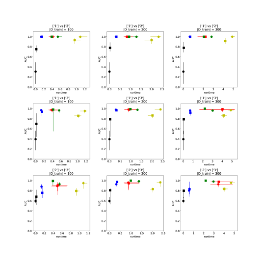
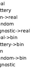
Figure 6: Runtime and performance of different training strategies and different tasks. The size of the training data set and the class names of each experiment are indicated on the title of each plots.

C.2 MNIST: multi-class experiments

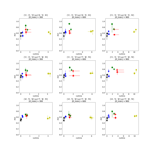
Figure 7: Runtime and performance of different training strategies and different tasks. The size of the training data set and the class names of each experiment are indicated on the title of each plots.

C.3 Citeseer: single-class experiments

Figure 8: Runtime and performance of different training strategies and different tasks. The size of the training data set and the class names of each experiment are indicated on the title of each plots.

C.4 Citeseer: multi-class experiments

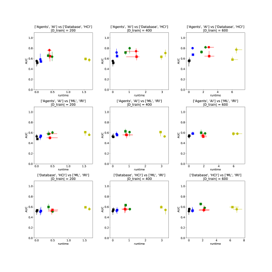
Figure 9: Runtime and performance of different training strategies and different tasks. The size of the training data set and the class names of each experiment are indicated on the title of each plots.

Appendix D More Laplacian spectra

D.1 Mnist: single-class experiments

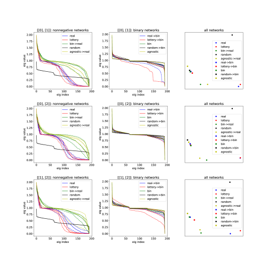
Figure 10: Spectrum of the normalized Laplacian matrix of real and binary models trained on different tasks. The size of the training data set is 150 images per class and the class names are indicated on the title of each plots.

References

- (1) Wenlin Chen, James Wilson, Stephen Tyree, Kilian Weinberger, and Yixin Chen. Compressing neural networks with the hashing trick. In International conference on machine learning, pages 2285–2294, 2015.
- (2) Maxwell D Collins and Pushmeet Kohli. Memory bounded deep convolutional networks. arXiv preprint arXiv:1412.1442, 2014.
- (3) Matthieu Courbariaux, Yoshua Bengio, and Jean-Pierre David. BinaryConnect: Training deep neural networks with binary weights during propagations. In Advances in neural information processing systems, pages 3123–3131, 2015.
- (4) Matthieu Courbariaux, Itay Hubara, Daniel Soudry, Ran El-Yaniv, and Yoshua Bengio. Binarized neural networks: Training deep neural networks with weights and activations constrained to+ 1 or-1. arXiv preprint arXiv:1602.02830, 2016.
- (5) Siemon de Lange, Marcel de Reus, and Martijn Van Den Heuvel. The laplacian spectrum of neural networks. Frontiers in computational neuroscience, 7:189, 2014.
- (6) Jacob Devlin, Ming-Wei Chang, Kenton Lee, and Kristina Toutanova. Bert: Pre-training of deep bidirectional transformers for language understanding. In Proceedings of the 2019 Conference of the North American Chapter of the Association for Computational Linguistics: Human Language Technologies, Volume 1 (Long and Short Papers), pages 4171–4186, 2019.
- (7) Jonathan Frankle and Michael Carbin. The lottery ticket hypothesis: Finding sparse, trainable neural networks. arXiv: Learning, 2019.
- (8) Adam Gaier and David Ha. Weight agnostic neural networks. In Advances in Neural Information Processing Systems, pages 5365–5379, 2019.
- (9) Alex Graves. Supervised sequence labelling. In Supervised sequence labelling with recurrent neural networks, pages 5–13. Springer, 2012.
- (10) Song Han, Huizi Mao, and William J Dally. Deep compression: Compressing deep neural networks with pruning, trained quantization and huffman coding. arXiv preprint arXiv:1510.00149, 2015.
- (11) Song Han, Jeff Pool, John Tran, and William J. Dally. Learning both weights and connections for efficient neural network. ArXiv, abs/1506.02626, 2015.
- (12) Qinghao Hu, Peisong Wang, and Jian Cheng. From hashing to cnns: Training binary weight networks via hashing. In Thirty-Second AAAI Conference on Artificial Intelligence, 2018.
- (13) Itay Hubara, Matthieu Courbariaux, Daniel Soudry, Ran El-Yaniv, and Yoshua Bengio. Quantized neural networks: Training neural networks with low precision weights and activations. The Journal of Machine Learning Research, 18(1):6869–6898, 2017.
- (14) Benoit Jacob, Skirmantas Kligys, Bo Chen, Menglong Zhu, Matthew Tang, Andrew Howard, Hartwig Adam, and Dmitry Kalenichenko. Quantization and training of neural networks for efficient integer-arithmetic-only inference. In Proceedings of the IEEE Conference on Computer Vision and Pattern Recognition, pages 2704–2713, 2018.
- (15) Hanxiao Liu, Karen Simonyan, and Yiming Yang. DARTS: Differentiable architecture search. arXiv preprint arXiv:1806.09055, 2018.
- (16) Xuezhe Ma and Eduard Hovy. End-to-end sequence labeling via bi-directional lstm-cnns-crf. In Proceedings of the 54th Annual Meeting of the Association for Computational Linguistics (Volume 1: Long Papers), pages 1064–1074, 2016.
- (17) Hieu Pham, Melody Y Guan, Barret Zoph, Quoc V Le, and Jeff Dean. Efficient neural architecture search via parameter sharing. arXiv preprint arXiv:1802.03268, 2018.
- (18) Esteban Real, Alok Aggarwal, Yanping Huang, and Quoc V Le. Regularized evolution for image classifier architecture search. In Proceedings of the AAAI conference on artificial intelligence, volume 33, pages 4780–4789, 2019.
- (19) M. Reuter, M. Niethammer, F. Wolter, S. Bouix, and M. Shenton. Global medical shape analysis using the volumetric laplace spectrum. In 2007 International Conference on Cyberworlds (CW’07), pages 417–426, 2007.
- (20) Mingzhu Shen, Kai Han, Chunjing Xu, and Yunhe Wang. Searching for accurate binary neural architectures. In Proceedings of the IEEE International Conference on Computer Vision Workshops, pages 0–0, 2019.
- (21) Daniel Soudry, Itay Hubara, and Ron Meir. Expectation backpropagation: Parameter-free training of multilayer neural networks with continuous or discrete weights. In Advances in Neural Information Processing Systems, pages 963–971, 2014.
- (22) Kenneth O Stanley and Risto Miikkulainen. Evolving neural networks through augmenting topologies. Evolutionary computation, 10(2):99–127, 2002.
- (23) Christian Szegedy, Sergey Ioffe, Vincent Vanhoucke, and Alexander A Alemi. Inception-v4, inception-resnet and the impact of residual connections on learning. In Thirty-first AAAI conference on artificial intelligence, 2017.
- (24) Ashish Vaswani, Noam Shazeer, Niki Parmar, Jakob Uszkoreit, Llion Jones, Aidan N Gomez, Łukasz Kaiser, and Illia Polosukhin. Attention is all you need. In Advances in neural information processing systems, pages 5998–6008, 2017.
- (25) Pablo Villegas, Paolo Moretti, and Miguel A Munoz. Frustrated hierarchical synchronization and emergent complexity in the human connectome network. Scientific reports, 4:5990, 2014.
- (26) Yunchao Wei, Wei Xia, Min Lin, Junshi Huang, Bingbing Ni, Jian Dong, Yao Zhao, and Shuicheng Yan. Hcp: A flexible cnn framework for multi-label image classification. IEEE transactions on pattern analysis and machine intelligence, 38(9):1901–1907, 2015.
- (27) Sirui Xie, Hehui Zheng, Chunxiao Liu, and Liang Lin. Snas: stochastic neural architecture search. In International Conference on Learning Representations, 2019.
- (28) Shan You, Tao Huang, Mingmin Yang, Fei Wang, Chen Qian, and Changshui Zhang. Greedynas: Towards fast one-shot nas with greedy supernet. arXiv preprint arXiv:2003.11236, 2020.
- (29) Haonan Yu, Sergey Edunov, Yuandong Tian, and Ari S Morcos. Playing the lottery with rewards and multiple languages: lottery tickets in rl and nlp. arXiv preprint arXiv:1906.02768, 2019.
- (30) Yuge Zhang, Zejun Lin, Junyang Jiang, Quanlu Zhang, Yujing Wang, Hui Xue, Chen Zhang, and Yaming Yang. Deeper insights into weight sharing in neural architecture search. arXiv preprint arXiv:2001.01431, 2020.
- (31) Hattie Zhou, Janice Lan, Rosanne Liu, and Jason Yosinski. Deconstructing lottery tickets: Zeros, signs, and the supermask. In NeurIPS, 2019.
- (32) Shuchang Zhou, Yuxin Wu, Zekun Ni, Xinyu Zhou, He Wen, and Yuheng Zou. Dorefa-net: Training low bitwidth convolutional neural networks with low bitwidth gradients. arXiv preprint arXiv:1606.06160, 2016.
- (33) Barret Zoph and Quoc V Le. Neural architecture search with reinforcement learning. arXiv preprint arXiv:1611.01578, 2016.