Effective nonlocal kernels on Reaction-diffusion networks 111 This work was supported in part by JST CREST (No. JPMJCR14D3) to S.-I. E., JSPS KAKENHI (No. 17K14228) to Y. T.

Shin-Ichiro Ei Eichiro@math.sci.hokudai.ac.jp Hiroshi Ishii hiroshi-ishii@eis.hokudai.ac.jp Shigeru Kondo skondo@fbs.osaka-u.ac.jp Takashi Miura miura_t@anat1.med.kyushu-u.ac.jp Yoshitaro Tanaka yoshitaro.tanaka@gmail.com Department of Mathematics, Faculty of Science, Hokkaido University Graduate School of Frontier Biosciences, Osaka University Graduate School of Medical Sciences, Kyushu University School of Systems Information Science, Future University Hakodate
Abstract

A new method to derive an essential integral kernel from any given reaction-diffusion network is proposed. Any network describing metabolites or signals with arbitrary many factors can be reduced to a single or a simpler system of integro-differential equations called “effective equation” including the reduced integral kernel (called “effective kernel” ) in the convolution type. As one typical example, the Mexican hat shaped kernel is theoretically derived from two component activator-inhibitor systems. It is also shown that a three component system with quite different appearance from activator-inhibitor systems is reduced to an effective equation with the Mexican hat shaped kernel. It means that the two different systems have essentially the same effective equations and that they exhibit essentially the same spatial and temporal patterns. Thus, we can identify two different systems with the understanding in unified concept through the reduced effective kernels. Other two applications of this method are also given: Applications to pigment patterns on skins (two factors network with long range interaction) and waves of differentiation (called proneural waves) in visual systems on brains (four factors network with long range interaction) . In the applications, we observe the reproduction of the same spatial and temporal patterns as those appearing in pre-existing models through the numerical simulations of the effective equations.

keywords:
non-local convolution , pattern formation , network , reaction-diffusion , Turing pattern
45K05 , 35Q92 , 92C42

1 Introduction

The understanding of the mechanism for self-organization is one of the most attractive and important themes in biology. Diffusion driven instability proposed by Turing [21] has given a significant part of the theoretical basement which has been adapted by many works related to pattern formation problems (Meinhardt [11], Murray [13]). In practice, the existence of the mechanism in real nature has been observed and checked for several real phenomena (e.g. Ouyang and Swinney [17], Kondo and Asai [9], Yamaguchi et.al. [23]). The mechanism of the diffusion driven instability was understood as the interaction between the slow diffusivity of short range self-enhancing activator and the fast one of long range inhibitor or simply “ local activation with long-range inhibition (LALI)” (e.g. Gierer-Meinhardt [7], Oster [16]) as in Fig.1. The situation is frequently modeled in the form of reaction-diffusion systems with two components of the activator u=u(t,x)𝑢𝑢𝑡𝑥u=u(t,x) and the inhibitor v=v(t,x)𝑣𝑣𝑡𝑥v=v(t,x) at time t>0𝑡0t>0 and position x𝑥x

{ut=d1Δu+f(u,v),vt=d2Δv+g(u,v),casessubscript𝑢𝑡subscript𝑑1Δ𝑢𝑓𝑢𝑣subscript𝑣𝑡subscript𝑑2Δ𝑣𝑔𝑢𝑣\left\{\begin{array}[]{ccl}u_{t}&=&d_{1}\Delta u+f(u,v),\\ v_{t}&=&d_{2}\Delta v+g(u,v),\end{array}\right. (1.1)

which is called Activator-Inhibitor system. In (1.1), ΔΔ\Delta denotes the Laplace operator and it is assumed that the diffusion coefficients 0<d1<d20subscript𝑑1subscript𝑑20<d_{1}<d_{2} and the nonlinear terms fu>0subscript𝑓𝑢0f_{u}>0, fv<0subscript𝑓𝑣0f_{v}<0, gu>0subscript𝑔𝑢0g_{u}>0 and gv<0subscript𝑔𝑣0g_{v}<0. The typical example of f𝑓f and g𝑔g are f(u,v)=c1uc2v𝑓𝑢𝑣subscript𝑐1𝑢subscript𝑐2𝑣f(u,v)=c_{1}u-c_{2}v and g(u,v)=c3uc4v𝑔𝑢𝑣subscript𝑐3𝑢subscript𝑐4𝑣g(u,v)=c_{3}u-c_{4}v with all positive constants cj,(j=1,,4)subscript𝑐𝑗𝑗14c_{j},(j=1,\cdots,4), which appear as a linear approximation in the neighbourhood of an equilibrium. In fact, the diffusion driven instability is understood for the linearized system as follows: Let the linearized system for an equilibrium, say 0, be

{ut=d1Δu+c1uc2v,vt=d2Δv+c3uc4v.casessubscript𝑢𝑡subscript𝑑1Δ𝑢subscript𝑐1𝑢subscript𝑐2𝑣subscript𝑣𝑡subscript𝑑2Δ𝑣subscript𝑐3𝑢subscript𝑐4𝑣\left\{\begin{array}[]{ccl}u_{t}&=&d_{1}\Delta u+c_{1}u-c_{2}v,\\ v_{t}&=&d_{2}\Delta v+c_{3}u-c_{4}v.\end{array}\right. (1.2)

For the simplicity, we consider (1.2) on 𝐑𝟏superscript𝐑1\bf R^{1}. Then the Fourier transformation of (1.2) yields

{u^t=d1ξ2u^+c1u^c2v^,v^t=d2ξ2v^+c3u^c4v^casessubscript^𝑢𝑡subscript𝑑1superscript𝜉2^𝑢subscript𝑐1^𝑢subscript𝑐2^𝑣subscript^𝑣𝑡subscript𝑑2superscript𝜉2^𝑣subscript𝑐3^𝑢subscript𝑐4^𝑣\left\{\begin{array}[]{ccl}\widehat{u}_{t}&=&-d_{1}\xi^{2}\widehat{u}+c_{1}\widehat{u}-c_{2}\widehat{v},\\ \widehat{v}_{t}&=&-d_{2}\xi^{2}\widehat{v}+c_{3}\widehat{u}-c_{4}\widehat{v}\end{array}\right. (1.3)

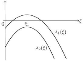
while the specific notations are defined in Section 2. That is, (1.3) is written as U^t=B(ξ)U^subscript^𝑈𝑡𝐵𝜉^𝑈\widehat{U}_{t}=B(\xi)\widehat{U} with U^:=(u^v^)assign^𝑈^𝑢^𝑣\widehat{U}:=\left(\begin{array}[]{c}\widehat{u}\\ \widehat{v}\end{array}\right) and B(ξ):=(d1ξ2+c1c2c3d2ξ2c4)assign𝐵𝜉subscript𝑑1superscript𝜉2subscript𝑐1subscript𝑐2subscript𝑐3subscript𝑑2superscript𝜉2subscript𝑐4B(\xi):=\left(\begin{array}[]{cc}-d_{1}\xi^{2}+c_{1}&-c_{2}\\ c_{3}&-d_{2}\xi^{2}-c_{4}\end{array}\right). Denoting the eigenvalues of B(ξ)𝐵𝜉B(\xi) by λ1(ξ)subscript𝜆1𝜉\lambda_{1}(\xi), λ2(ξ)subscript𝜆2𝜉\lambda_{2}(\xi) with λ1(0)λ2(0)subscript𝜆10subscript𝜆20\lambda_{1}(0)\geq\lambda_{2}(0) and defining λmax(ξ):=max{λ1(ξ),λ2(ξ)}assignsubscript𝜆𝑚𝑎𝑥𝜉subscript𝜆1𝜉subscript𝜆2𝜉\lambda_{max}(\xi):=\max\{\lambda_{1}(\xi),\lambda_{2}(\xi)\}, we assume the maximal eigenvalue λmax(ξ)subscript𝜆𝑚𝑎𝑥𝜉\lambda_{max}(\xi) satisfies λmax(0)<0subscript𝜆𝑚𝑎𝑥00\lambda_{max}(0)<0 and λmax(ξ1)>0subscript𝜆𝑚𝑎𝑥subscript𝜉10\lambda_{max}(\xi_{1})>0 for ξ1>0subscript𝜉10\xi_{1}>0 as in Fig.2. When the assumption for λmax(ξ)subscript𝜆𝑚𝑎𝑥𝜉\lambda_{max}(\xi) holds, it is called “the diffusion driven instability” or “Turing Instability”.

Refer to caption
Figure 1: Activator-Inhibitor network. \rightarrow and does-not-prove\dashv denote activation and inhibition, respectively.
Refer to caption
Figure 2: Schematic graphs of λ1(ξ)subscript𝜆1𝜉\lambda_{1}(\xi) and λ2(ξ)subscript𝜆2𝜉\lambda_{2}(\xi). In this case, λmax(ξ)=λ1(ξ)subscript𝜆𝑚𝑎𝑥𝜉subscript𝜆1𝜉\lambda_{max}(\xi)=\lambda_{1}(\xi) holds.

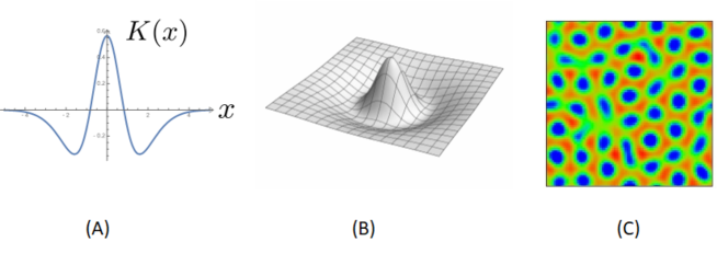
Recently, Kondo [8] suggested that the activator-inhibitor system is equivalent to a kernel-based model with the Mexican hat kernel which is a function defined by regarding locally positive and spreading negative parts as a local activation and a lateral inhibition, respectively as in Fig.3 for x𝐑𝑥𝐑x\in\bf R or 𝐱𝐑𝟐𝐱superscript𝐑2\bf x\in\bf R^{2}. Kondo proposed the following model with convolution (for the definition, see Section 2) by using an integral kernel K𝐾K

ut=χ(Ku)αu,subscript𝑢𝑡𝜒𝐾𝑢𝛼𝑢u_{t}=\chi(K*u)-\alpha u, (1.4)

where χ(r):={0,r0,r,0<rr,r,rrassign𝜒𝑟cases0𝑟0𝑟0𝑟superscript𝑟superscript𝑟𝑟superscript𝑟\chi(r):=\left\{\begin{array}[]{cc}0,&r\leq 0,\\ r,&0<r\leq r^{*},\\ r^{*},&r\geq r^{*}\end{array}\right. for a positive constant rsuperscript𝑟r^{*} and the integral kernel function K=K(|𝐱|)𝐾𝐾𝐱K=K(|\bf x|) is a radially symmetric function with Mexican hat profiles or other general functions.
Refer to caption
Figure 3: Integral kernels K𝐾K with the Mexican hat profile. (A) is on 𝐑𝐑{\bf R}, (B) is on 𝐑2superscript𝐑2{\bf R}^{2}, (C) is the numerically generated 2D patterns with Mexican hat kernel of (B).

The Mexican hat shaped kernel K𝐾K was given in [8] as the sum of two Gaussian functions and numerically showed the self-organization of spatially periodic 2D patterns similar to those appearing in the activator-inhibitor reaction diffusion systems can be reproduced in (1.4). In practice, the Fourier transformation of the kernel leads the dispersion relation of (1.4) and the existence of a unstable nonzero wave number is easily checked, that is, it has a similar structure of Turing Instability. In that sense, the kernel-based model like (1.4) is called “Kernel-based Turing model (KT model)” in Kondo ([8]).

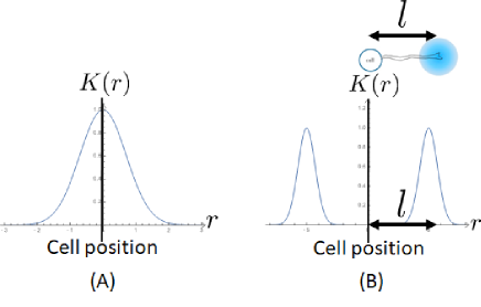
KT models in the type of (1.4) are very effective to investigate spatially appearing patterns. One reason is that we do not need to know underlying mechanisms of molecules or cells in detail and that the kernel shape is detected directly from an experimental observation as stated in Kondo [8]. In fact, Kuffler [10] detected the kernel shape related to mammalian retina directly from the observation in real experiments. For example, the diffusion process is phenomenologically expressed by a unimodal localized profile of the kernel with one peak at the center as in Fig.4(A), whose relation was rigorously proved in Bates et. al. [2, 3], and the cell projection which releases the signal molecule at the specific position is by a kernel of a profile with peaks l𝑙l distant from the center as in Fig.4(B).

Another reason is that KT models can easily reproduce more complicated patterns which are difficult to show by conventional two component reaction diffusion systems such as nested patterns appearing often on animal skins and sea shells. Such complicated patterns were numerically demonstrated in [8] by using several other types of kernel functions.
Refer to caption
Figure 4: Examples of kernel shapes. (A) corresponds to diffusion process with the peak at the center (r=0𝑟0r=0). (B) is the kernel shape by cell projections with peaks l𝑙l distant from the center.

Thus, spatial patterns and kernel shapes are directly related while kernel shapes are related to the background mechanisms of molecular or cellular processes together with the signal or metabolic networks. It means the possibility of two step approach toward the theoretical understanding of spatial patterns, that is, one is the research into the relation between patterns and kernel shapes which corresponds to the macroscopic researches, another is between kernel shapes and underlying biological mechanisms which corresponds to microscopic ones. Thus, KT models can connect macroscopic structures and microscopic ones through the kernels and this two step approach has a big advantage because these two steps can be treated independently and separately.

Model equations of the type of (1.4) have been proposed in many fields such as neural system (e.g. Amari[1], Murray[13] ), cell-cell adhesion problem (e.g. Carrillo et. al.[5], Painter et. al.[18] ), Optical illusion (Sushida et. al. [19] ). Recently, integral kernels were also used to the development of the continuous method for spatially discrete models ([6]).

In all of them, appropriate integral kernels were adopted from the phenomenological point of view such as the direct detection from the experiments (e.g. Kuffler[10]). In that sense, they can be regarded as works in the step for the relation between patterns and kernel shapes. On the other hand, there have been almost no works in the step between kernel shapes and underlying biological mechanisms while both steps are absolutely necessary to understand the whole mechanism from micro to macro structures.

In this paper, we consider the relation between kernel shapes and the local networks of metabolites or signals as underlying microscopic mechanisms, and propose a new method to derive an effective kernel shape from an arbitrarily given network. Since the spatial and temporal patterns are essentially governed by the effective equation with the effective kernel, it can give us a unified aspect through the derived effective kernel between seemingly different network systems. Actually, we can identify seemingly different network systems when the effective equations are same.

As one typical example of our approach, let us consider the activator-inhibitor system with the local network like Fig.1, which is basically described by the reaction diffusion system (1.1). As stated in Meinhardt and Gierer ([7]), the essential effect of this system is the property of “local activation with long-range inhibition (LALI)” and it has been believed that the corresponding kernel shape is the Mexican hat profile as in Fig.3. But there have been no theoretical investigation between the kernel shape of the Mexican hat profile and the activator-inhibitor system (1.1). By applying our technique, we systematically derive the Mexican hat shaped kernel from (1.2). The details are shown in Section 3 together with the basic idea of this technique.

We also demonstrate our technique in Section 5 by applying to models with complicated networks including 3 components models in [14], pigment patterns on skins with projections in [15] and regulating waves of differentiation in [20].

For the convenience of readers, we summarize notations and results of the Fourier transformation in Section 2.

2 Preliminaries of the Fourier transformation

In this section, we give several notations and definitions for the Fourier transformation as follows:
For a function f(x)𝑓𝑥f(x) on 𝐑𝐑\bf R, the Fourier transformation of f𝑓f is defined by

f^(ξ)=(f)(ξ):=f(x)eixξ𝑑x^𝑓𝜉𝑓𝜉assignsuperscriptsubscript𝑓𝑥superscript𝑒𝑖𝑥𝜉differential-d𝑥\hat{f}(\xi)=({\cal F}f)(\xi):=\displaystyle\int_{-\infty}^{\infty}f(x)e^{-ix\xi}dx

and the inverse Fourier transformation is

fˇ(x)=(1f)(x):=12πf(ξ)eiξx𝑑ξ.ˇ𝑓𝑥superscript1𝑓𝑥assign12𝜋superscriptsubscript𝑓𝜉superscript𝑒𝑖𝜉𝑥differential-d𝜉\check{f}(x)=({\cal F}^{-1}f)(x):=\displaystyle\frac{1}{2\pi}\displaystyle\int_{-\infty}^{\infty}f(\xi)e^{i\xi x}d\xi.

In particular,

(1f)(x)=1π0f(ξ2)cosξxdξsuperscript1𝑓𝑥1𝜋superscriptsubscript0𝑓superscript𝜉2𝜉𝑥𝑑𝜉({\cal F}^{-1}f)(x)=\displaystyle\frac{1}{\pi}\displaystyle\int_{0}^{\infty}f(\xi^{2})\cos\xi xd\xi (2.1)

holds for f=f(ξ2)𝑓𝑓superscript𝜉2f=f(\xi^{2}). The convolution of f𝑓f and g𝑔g is defined by

(fg)(x):=f(xy)g(y)𝑑y=f(y)g(xy)𝑑yassign𝑓𝑔𝑥superscriptsubscript𝑓𝑥𝑦𝑔𝑦differential-d𝑦superscriptsubscript𝑓𝑦𝑔𝑥𝑦differential-d𝑦(f*g)(x):=\displaystyle\int_{-\infty}^{\infty}f(x-y)g(y)dy=\displaystyle\int_{-\infty}^{\infty}f(y)g(x-y)dy

and fg^=f^g^^𝑓𝑔^𝑓^𝑔\widehat{f*g}=\hat{f}\cdot\hat{g} holds.

For a function f(x,y)𝑓𝑥𝑦f(x,y) on 𝐑𝟐superscript𝐑2\bf R^{2}, the Fourier transformation is defined by

f^(ξ,η)=(f)(ξ,η):=f(x,y)ei(xξ+yη)𝑑x𝑑y^𝑓𝜉𝜂𝑓𝜉𝜂assignsuperscriptsubscriptsuperscriptsubscript𝑓𝑥𝑦superscript𝑒𝑖𝑥𝜉𝑦𝜂differential-d𝑥differential-d𝑦\hat{f}(\xi,\eta)=({\cal F}f)(\xi,\eta):=\displaystyle\int_{-\infty}^{\infty}\!\displaystyle\int_{-\infty}^{\infty}f(x,y)e^{-i(x\xi+y\eta)}dxdy

and the inverse Fourier transformation is

fˇ(x,y)=(1f)(x,y):=1(2π)2f(ξ,η)ei(ξx+ηy)𝑑ξ𝑑η.ˇ𝑓𝑥𝑦superscript1𝑓𝑥𝑦assign1superscript2𝜋2superscriptsubscriptsuperscriptsubscript𝑓𝜉𝜂superscript𝑒𝑖𝜉𝑥𝜂𝑦differential-d𝜉differential-d𝜂\check{f}(x,y)=({\cal F}^{-1}f)(x,y):=\displaystyle\frac{1}{(2\pi)^{2}}\displaystyle\int_{-\infty}^{\infty}\!\displaystyle\int_{-\infty}^{\infty}f(\xi,\eta)e^{i(\xi x+\eta y)}d\xi d\eta.

The convolution of f𝑓f and g𝑔g is

(fg)(x,y):=f(xx,yy)g(x,y)𝑑x𝑑yassign𝑓𝑔𝑥𝑦superscriptsubscriptsuperscriptsubscript𝑓𝑥superscript𝑥𝑦superscript𝑦𝑔superscript𝑥superscript𝑦differential-dsuperscript𝑥differential-dsuperscript𝑦(f*g)(x,y):=\displaystyle\int_{-\infty}^{\infty}\displaystyle\int_{-\infty}^{\infty}f(x-x^{\prime},y-y^{\prime})g(x^{\prime},y^{\prime})dx^{\prime}dy^{\prime}

and fg^=f^g^^𝑓𝑔^𝑓^𝑔\widehat{f*g}=\hat{f}\cdot\hat{g} holds.

In particular, for a radially symmetric function K=K(r)𝐾𝐾𝑟K=K(r) with r:=x2+y2assign𝑟superscript𝑥2superscript𝑦2r:=\sqrt{x^{2}+y^{2}}, the Fourier transformation of K𝐾K is computed by polar coordinate

K^(ξ,η)^𝐾𝜉𝜂\displaystyle\hat{K}(\xi,\eta) =\displaystyle= K(x2+y2)ei(ξx+ηy)𝑑x𝑑ysuperscriptsubscriptsuperscriptsubscript𝐾superscript𝑥2superscript𝑦2superscript𝑒𝑖𝜉𝑥𝜂𝑦differential-d𝑥differential-d𝑦\displaystyle\displaystyle\int_{-\infty}^{\infty}\!\displaystyle\int_{-\infty}^{\infty}K(\sqrt{x^{2}+y^{2}})e^{-i(\xi x+\eta y)}dxdy
=\displaystyle= 002πrK(r)eir(ξcosθ+ηsinθ)𝑑r𝑑θsuperscriptsubscript0superscriptsubscript02𝜋𝑟𝐾𝑟superscript𝑒𝑖𝑟𝜉𝜃𝜂𝜃differential-d𝑟differential-d𝜃\displaystyle\displaystyle\int_{0}^{\infty}\!\displaystyle\int_{0}^{2\pi}rK(r)e^{-ir(\xi\cos\theta+\eta\sin\theta)}drd\theta
=\displaystyle= 002πrK(r)eirRcos(θα)𝑑r𝑑θsuperscriptsubscript0superscriptsubscript02𝜋𝑟𝐾𝑟superscript𝑒𝑖𝑟𝑅𝜃𝛼differential-d𝑟differential-d𝜃\displaystyle\displaystyle\int_{0}^{\infty}\!\displaystyle\int_{0}^{2\pi}rK(r)e^{-irR\cos(\theta-\alpha)}drd\theta
=\displaystyle= 002πrK(r)eirRcosθ𝑑r𝑑θ,superscriptsubscript0superscriptsubscript02𝜋𝑟𝐾𝑟superscript𝑒𝑖𝑟𝑅𝜃differential-d𝑟differential-d𝜃\displaystyle\displaystyle\int_{0}^{\infty}\!\displaystyle\int_{0}^{2\pi}rK(r)e^{-irR\cos\theta}drd\theta,

where R:=ξ2+η2assign𝑅superscript𝜉2superscript𝜂2R:=\sqrt{\xi^{2}+\eta^{2}} and α=α(ξ,η)𝛼𝛼𝜉𝜂\alpha=\alpha(\xi,\eta). That is, K^^𝐾\hat{K} is also radially symmetric and computed as

K^(R)^𝐾𝑅\displaystyle\hat{K}(R) =\displaystyle= 002πrK(r)eirRcosθ𝑑r𝑑θsuperscriptsubscript0superscriptsubscript02𝜋𝑟𝐾𝑟superscript𝑒𝑖𝑟𝑅𝜃differential-d𝑟differential-d𝜃\displaystyle\displaystyle\int_{0}^{\infty}\!\!\!\!\displaystyle\int_{0}^{2\pi}rK(r)e^{-irR\cos\theta}drd\theta (2.2)
=\displaystyle= 200πrK(r)cos(rRsinθ)𝑑θ𝑑r2superscriptsubscript0superscriptsubscript0𝜋𝑟𝐾𝑟𝑟𝑅𝜃differential-d𝜃differential-d𝑟\displaystyle 2\displaystyle\int_{0}^{\infty}\!\!\!\!\displaystyle\int_{0}^{\pi}rK(r)\cos(rR\sin\theta)d\theta dr
=\displaystyle= 400π/2rK(r)cos(rRsinθ)𝑑θ𝑑r.4superscriptsubscript0superscriptsubscript0𝜋2𝑟𝐾𝑟𝑟𝑅𝜃differential-d𝜃differential-d𝑟\displaystyle 4\!\displaystyle\int_{0}^{\infty}\!\!\!\!\displaystyle\int_{0}^{\pi/2}\!\!\!\!\!\!rK(r)\cos(rR\sin\theta)d\theta dr.

Similarly, the inverse Fourier transformation for a radially symmetric function K(R)𝐾𝑅K(R) is

Kˇ(r)ˇ𝐾𝑟\displaystyle\check{K}(r) =\displaystyle= 1(2π)2002πRK(R)eirRcosθ𝑑R𝑑θ1superscript2𝜋2superscriptsubscript0superscriptsubscript02𝜋𝑅𝐾𝑅superscript𝑒𝑖𝑟𝑅𝜃differential-d𝑅differential-d𝜃\displaystyle\displaystyle\frac{1}{(2\pi)^{2}}\displaystyle\int_{0}^{\infty}\!\!\!\!\displaystyle\int_{0}^{2\pi}RK(R)e^{irR\cos\theta}dRd\theta (2.3)
=\displaystyle= 12π200πRK(R)cos(rRsinθ)𝑑θ𝑑R12superscript𝜋2superscriptsubscript0superscriptsubscript0𝜋𝑅𝐾𝑅𝑟𝑅𝜃differential-d𝜃differential-d𝑅\displaystyle\displaystyle\frac{1}{2\pi^{2}}\displaystyle\int_{0}^{\infty}\!\!\!\!\displaystyle\int_{0}^{\pi}RK(R)\cos(rR\sin\theta)d\theta dR
=\displaystyle= 1π200π/2RK(R)cos(rRsinθ)𝑑θ𝑑R.1superscript𝜋2superscriptsubscript0superscriptsubscript0𝜋2𝑅𝐾𝑅𝑟𝑅𝜃differential-d𝜃differential-d𝑅\displaystyle\displaystyle\frac{1}{\pi^{2}}\displaystyle\int_{0}^{\infty}\!\!\!\!\displaystyle\int_{0}^{\pi/2}\!\!\!RK(R)\cos(rR\sin\theta)d\theta dR.

Here we give approximations of Dirac δ𝛿\delta function, say δ(x)𝛿𝑥\delta(x). In general, the following proposition holds.

Proposition 2.1.

(Approximation of δ(x)𝛿𝑥\delta(x))
Suppose Gϵ(x)subscript𝐺italic-ϵ𝑥G_{\epsilon}(x) is a function satisfying
1)  Gϵ(x)0subscript𝐺italic-ϵ𝑥0G_{\epsilon}(x)\geq 0,
2)  𝐑Gϵ(x)𝑑x=1subscript𝐑subscript𝐺italic-ϵ𝑥differential-d𝑥1\displaystyle\int_{\bf R}G_{\epsilon}(x)dx=1,
3)  limϵ0|x|>ηGϵ(x)𝑑x=0subscriptitalic-ϵ0subscript𝑥𝜂subscript𝐺italic-ϵ𝑥differential-d𝑥0\displaystyle\lim_{\epsilon\downarrow 0}\displaystyle\int_{|x|>\eta}G_{\epsilon}(x)dx=0 for any η>0𝜂0\eta>0.
Then (Gϵu)(x)u(x)subscript𝐺italic-ϵ𝑢𝑥𝑢𝑥(G_{\epsilon}*u)(x)\rightarrow u(x) as ϵ0italic-ϵ0\epsilon\downarrow 0 holds, that is, Gϵδ(x)subscript𝐺italic-ϵ𝛿𝑥G_{\epsilon}\rightarrow\delta(x).

Typical examples of Gϵsubscript𝐺italic-ϵG_{\epsilon} are the heat kernel Hϵ(x):=14πϵex24ϵassignsubscript𝐻italic-ϵ𝑥14𝜋italic-ϵsuperscript𝑒superscript𝑥24italic-ϵH_{\epsilon}(x):=\displaystyle\frac{1}{\sqrt{4\pi\epsilon}}e^{-\frac{x^{2}}{4\epsilon}}, and a mollifier Jϵ(ξ)subscript𝐽italic-ϵ𝜉J_{\epsilon}(\xi) given by Jϵ(x):=1ϵJ(xϵ)assignsubscript𝐽italic-ϵ𝑥1italic-ϵ𝐽𝑥italic-ϵJ_{\epsilon}(x):=\frac{1}{\epsilon}J(\frac{x}{\epsilon}) for a function J(x)𝐽𝑥J(x) satisfying J(x)0𝐽𝑥0J(x)\geq 0, 𝐑J(x)𝑑x=1subscript𝐑𝐽𝑥differential-d𝑥1\displaystyle\int_{\bf R}J(x)dx=1 and J(x)=0𝐽𝑥0J(x)=0 for |x|1𝑥1|x|\geq 1. In this paper, we furthermore impose the condition J^(ξ)0^𝐽𝜉0\widehat{J}(\xi)\geq 0 in order to keep the order of eigenvalues while the condition is not required in general. Such a function J(x)𝐽𝑥J(x) is for example made by J(x)={jj}(x)𝐽𝑥𝑗𝑗𝑥J(x)=\{j*j\}(x) for a function j(x)𝑗𝑥j(x). Then J^(ξ)={j^(ξ)}20^𝐽𝜉superscript^𝑗𝜉20\widehat{J}(\xi)=\{\widehat{j}(\xi)\}^{2}\geq 0 holds while Hϵ^(ξ)=eϵξ2>0^subscript𝐻italic-ϵ𝜉superscript𝑒italic-ϵsuperscript𝜉20\widehat{H_{\epsilon}}(\xi)=e^{-\epsilon\xi^{2}}>0 holds. Since the mollifier Jϵ(x)subscript𝐽italic-ϵ𝑥J_{\epsilon}(x) satisfies (Jϵu)(x)=0subscript𝐽italic-ϵ𝑢𝑥0(J_{\epsilon}*u)(x)=0 outside of ϵlimit-fromitalic-ϵ\epsilon- neighborhood of the support of u(x)𝑢𝑥u(x), that is, supp(Jϵu)Wϵ(supp(u))𝑠𝑢𝑝𝑝subscript𝐽italic-ϵ𝑢subscript𝑊italic-ϵ𝑠𝑢𝑝𝑝𝑢supp(J_{\epsilon}*u)\subset W_{\epsilon}(supp(u)) holds for Wϵ(supp(u)):={x+y;xsupp(u),|y|ϵ}W_{\epsilon}(supp(u)):=\{x+y;\;x\in supp(u),\;|y|\leq\epsilon\}, it is useful when the support should be taken into account. Above properties for δ(x)𝛿𝑥\delta(x) will be used to compute several kernels in the following sections.

In the last of this section, we give several properties of the Lambert W function, say w=W(z)𝑤𝑊𝑧w=W(z), which is a root w𝑤w of the equation

wew=z.𝑤superscript𝑒𝑤𝑧we^{w}=z. (2.4)

Then we have:

Proposition 2.2.

1)  For z0𝑧0z\geq 0, (2.4) has a non-negative root w0(z)0subscript𝑤0𝑧0w_{0}(z)\geq 0 and any other root w𝑤w satisfies Re(w)<0𝑅𝑒𝑤0Re(w)<0.
2)  For 1/e<z<01𝑒𝑧0-1/e<z<0, (2.4) has two real roots w1(z)subscript𝑤1𝑧w_{1}(z), w2(z)subscript𝑤2𝑧w_{2}(z) (0>w1(z)>1>w2(z)0subscript𝑤1𝑧1subscript𝑤2𝑧0>w_{1}(z)>-1>w_{2}(z)) and any other root w𝑤w satisfies Re(w)<w1(z)𝑅𝑒𝑤subscript𝑤1𝑧Re(w)<w_{1}(z).
3)  For z=1/e𝑧1𝑒z=-1/e, (2.4) has the root w0=1subscript𝑤01w_{0}=-1 and any other root w𝑤w satisfies Re(w)<1𝑅𝑒𝑤1Re(w)<-1.

This propositon is referred to [4]. Here we express the principal branch of the Lambert W function by W0(z)subscript𝑊0𝑧W_{0}(z), which is given by W0(z)=w0𝐂subscript𝑊0𝑧subscript𝑤0𝐂W_{0}(z)=w_{0}\in{\bf C} satisfying Re(w0)=max{Re(w);wew=z}𝑅𝑒subscript𝑤0𝑅𝑒𝑤𝑤superscript𝑒𝑤𝑧Re(w_{0})=\max\{Re(w);\;we^{w}=z\}. It is noted by Proposition 2.2 that W0(z)subscript𝑊0𝑧W_{0}(z) is real for z1/e𝑧1𝑒z\geq-1/e satisfying W0(z)=w0(z)subscript𝑊0𝑧subscript𝑤0𝑧W_{0}(z)=w_{0}(z) for z0𝑧0z\geq 0 in 1), W0(z)=w1(z)subscript𝑊0𝑧subscript𝑤1𝑧W_{0}(z)=w_{1}(z) for 1/e<z<01𝑒𝑧0-1/e<z<0 in 2) and W0(1/e)=1subscript𝑊01𝑒1W_{0}(-1/e)=-1 in 3) of Proposition 2.2.

3 The basic idea and the theoretical derivation of the Mexican hat type kernel

In this section, we show our basic idea by using the activator-inhibitor system (1.2) (Fig.5) and theoretically derive the Mexican hat type kernel from it. For simplicity, we consider it on 𝐑𝐑{\bf R}.

The activator-inhibitor system has been represented by reaction diffusion systems, which have the following form in a linearized sense

{ut=d1uxx+c1uc2v,vt=d2vxx+c3uc4vcasessubscript𝑢𝑡subscript𝑑1subscript𝑢𝑥𝑥subscript𝑐1𝑢subscript𝑐2𝑣subscript𝑣𝑡subscript𝑑2subscript𝑣𝑥𝑥subscript𝑐3𝑢subscript𝑐4𝑣\left\{\begin{array}[]{ccl}u_{t}&=&d_{1}u_{xx}+c_{1}u-c_{2}v,\\ v_{t}&=&d_{2}v_{xx}+c_{3}u-c_{4}v\end{array}\right. (3.1)

for x𝐑𝑥𝐑x\in\bf R, where all coefficients d1subscript𝑑1d_{1}, d2subscript𝑑2d_{2} and cj(j=1,,4)subscript𝑐𝑗𝑗14c_{j}(j=1,\cdots,4) are positive and d1<d2subscript𝑑1subscript𝑑2d_{1}<d_{2}. (3.1) is written in a vector valued form

Ut=DUxx+AU,subscript𝑈𝑡𝐷subscript𝑈𝑥𝑥𝐴𝑈U_{t}=DU_{xx}+AU, (3.2)

where U=U(t,x):=(u(t,x)v(t,x))𝐑𝟐𝑈𝑈𝑡𝑥assign𝑢𝑡𝑥𝑣𝑡𝑥superscript𝐑2U=U(t,x):=\left(\begin{array}[]{c}u(t,x)\\ v(t,x)\end{array}\right)\in\bf R^{2}, D:=diag{d1,d2}=(d100d2)assign𝐷𝑑𝑖𝑎𝑔subscript𝑑1subscript𝑑2subscript𝑑100subscript𝑑2D:=diag\{d_{1},d_{2}\}=\left(\begin{array}[]{cc}d_{1}&0\\ 0&d_{2}\end{array}\right) and A:=(c1c2c3c4)assign𝐴subscript𝑐1subscript𝑐2subscript𝑐3subscript𝑐4A:=\left(\begin{array}[]{cc}c_{1}&-c_{2}\\ c_{3}&-c_{4}\end{array}\right). Here we note that variables u𝑢u and v𝑣v can take any sign since we consider solutions in the neighborhood of an equilibrium by the linearized equation like (3.1).

Refer to caption
Figure 5: The network of Activator-Inhibitor system. \rightarrow and does-not-prove\dashv denote activation and inhibition, respectively.

Taking the Fourier transformation of (3.2), we get

U^t=B(ξ)U^,subscript^𝑈𝑡𝐵𝜉^𝑈\widehat{U}_{t}=B(\xi)\widehat{U}, (3.3)

where B(ξ):=ξ2D+A=(d1ξ2+c1c2c3d2ξ2c4)assign𝐵𝜉superscript𝜉2𝐷𝐴subscript𝑑1superscript𝜉2subscript𝑐1subscript𝑐2subscript𝑐3subscript𝑑2superscript𝜉2subscript𝑐4B(\xi):=-\xi^{2}D+A=\left(\begin{array}[]{cc}-d_{1}\xi^{2}+c_{1}&-c_{2}\\ c_{3}&-d_{2}\xi^{2}-c_{4}\end{array}\right). Let λj(ξ)subscript𝜆𝑗𝜉\lambda_{j}(\xi) (j=1,2𝑗12j=1,2) be eigenvalues of B(ξ)𝐵𝜉B(\xi) and define λmax(ξ):=maxj{λj(ξ)}assignsubscript𝜆𝑚𝑎𝑥𝜉subscript𝑗subscript𝜆𝑗𝜉\lambda_{max}(\xi):=\displaystyle\max_{j}\{\lambda_{j}(\xi)\}.

Refer to caption
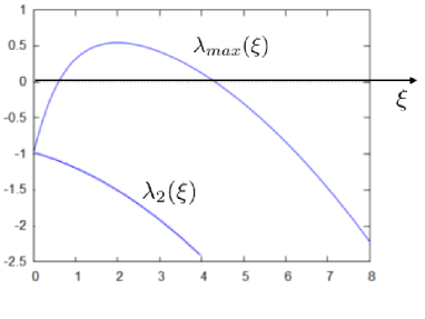
Figure 6: Eigenvalues λj(ξ)subscript𝜆𝑗𝜉\lambda_{j}(\xi) of B(ξ)𝐵𝜉B(\xi). c1=c2=1subscript𝑐1subscript𝑐21c_{1}=c_{2}=1, c3=4subscript𝑐34c_{3}=4, c4=3subscript𝑐43c_{4}=3, d1=0.05subscript𝑑10.05d_{1}=0.05 and d2=3subscript𝑑23d_{2}=3 in (3.1).

Here we compute the asymptotic profile of λmax(ξ)subscript𝜆𝑚𝑎𝑥𝜉\lambda_{max}(\xi) as |ξ|𝜉|\xi|\rightarrow\infty. When |λmax(ξ)λ±(ξ)|0subscript𝜆𝑚𝑎𝑥𝜉subscript𝜆plus-or-minus𝜉0|\lambda_{max}(\xi)-\lambda_{\pm\infty}(\xi)|\rightarrow 0 as ξ±𝜉plus-or-minus\xi\rightarrow\pm\infty, λ±(ξ)subscript𝜆plus-or-minus𝜉\lambda_{\pm\infty}(\xi) are called the “asymptotic profiles of λmax(ξ)subscript𝜆𝑚𝑎𝑥𝜉\lambda_{max}(\xi)” or the “asymptotic convergence to λ±(ξ)subscript𝜆plus-or-minus𝜉\lambda_{\pm\infty}(\xi)” as ξ±𝜉plus-or-minus\xi\rightarrow\pm\infty, which are expressed by λmax(ξ)λ±(ξ)subscript𝜆𝑚𝑎𝑥𝜉subscript𝜆plus-or-minus𝜉\lambda_{max}(\xi)\rightarrow\lambda_{\pm\infty}(\xi) as ξ±𝜉plus-or-minus\xi\rightarrow\pm\infty. In this example, λmax(ξ)subscript𝜆𝑚𝑎𝑥𝜉\lambda_{max}(\xi) has the asymptotic profile λmax(ξ)d1ξ2+c1subscript𝜆𝑚𝑎𝑥𝜉subscript𝑑1superscript𝜉2subscript𝑐1\lambda_{max}(\xi)\rightarrow-d_{1}\xi^{2}+c_{1} as |ξ|𝜉|\xi|\rightarrow\infty by virtue of d1<d2subscript𝑑1subscript𝑑2d_{1}<d_{2} as in Figures 2 and 6. Then we put λh(ξ):=d1ξ2assignsubscript𝜆𝜉subscript𝑑1superscript𝜉2\lambda_{h}(\xi):=-d_{1}\xi^{2} (taking the highest order term of ξ𝜉\xi) and put U^=etλh(ξ)V^^𝑈superscript𝑒𝑡subscript𝜆𝜉^𝑉\widehat{U}=e^{t\lambda_{h}(\xi)}\widehat{V}. We see that V^^𝑉\widehat{V} satisfies

V^t=Bh(ξ)V^,subscript^𝑉𝑡subscript𝐵𝜉^𝑉\widehat{V}_{t}=B_{h}(\xi)\widehat{V}, (3.4)

where Bh(ξ):=B(ξ)λh(ξ)I=(c1c2c3(d2d1)ξ2c4)assignsubscript𝐵𝜉𝐵𝜉subscript𝜆𝜉𝐼subscript𝑐1missing-subexpressionsubscript𝑐2subscript𝑐3missing-subexpressionsubscript𝑑2subscript𝑑1superscript𝜉2subscript𝑐4B_{h}(\xi):=B(\xi)-\lambda_{h}(\xi)I=\left(\begin{array}[]{ccc}c_{1}&&-c_{2}\\ c_{3}&&-(d_{2}-d_{1})\xi^{2}-c_{4}\end{array}\right) and I𝐼I is the identity matrix. We also divide Bhsubscript𝐵B_{h} into Bh(ξ)=ξB1(ξ)+B0(ξ)subscript𝐵𝜉𝜉subscript𝐵1𝜉subscript𝐵0𝜉B_{h}(\xi)=\xi B_{1}(\xi)+B_{0}(\xi) with B0(ξ)=O(1)subscript𝐵0𝜉𝑂1B_{0}(\xi)=O(1) as |ξ|𝜉|\xi|\rightarrow\infty, where B1(ξ)=(000(d2d1)ξ)subscript𝐵1𝜉0missing-subexpression00missing-subexpressionsubscript𝑑2subscript𝑑1𝜉B_{1}(\xi)=\left(\begin{array}[]{ccc}0&&0\\ 0&&-(d_{2}-d_{1})\xi\end{array}\right) and B0(ξ)=(c1c2c3c4)subscript𝐵0𝜉subscript𝑐1missing-subexpressionsubscript𝑐2subscript𝑐3missing-subexpressionsubscript𝑐4B_{0}(\xi)=\left(\begin{array}[]{ccc}c_{1}&&-c_{2}\\ c_{3}&&-c_{4}\end{array}\right) in this example. Since the Fourier transformation of the Dirac δ𝛿\delta-function is δ^(ξ)=1^𝛿𝜉1\widehat{\delta}(\xi)=1, we approximate it by the heat kernel Hε(x)subscript𝐻𝜀𝑥H_{\varepsilon}(x) as in Proposition 2.1 and modify Bh(ξ)subscript𝐵𝜉B_{h}(\xi) as Bε(ξ):=ξB1(ξ)+eεξ2B0(ξ)assignsubscript𝐵𝜀𝜉𝜉subscript𝐵1𝜉superscript𝑒𝜀superscript𝜉2subscript𝐵0𝜉B_{\varepsilon}(\xi):=\xi B_{1}(\xi)+e^{-\varepsilon\xi^{2}}B_{0}(\xi) for 0<ε<<10𝜀much-less-than10<\varepsilon<<1 by noting H^ε(ξ)=eεξ2subscript^𝐻𝜀𝜉superscript𝑒𝜀superscript𝜉2\widehat{H}_{\varepsilon}(\xi)=e^{-\varepsilon\xi^{2}}. We note that this modification is not necessary when |B0(ξ)|0subscript𝐵0𝜉0|B_{0}(\xi)|\rightarrow 0 as |ξ|𝜉|\xi|\rightarrow\infty. By using this modified matrix Bε(ξ)subscript𝐵𝜀𝜉B_{\varepsilon}(\xi), we consider

V^t=Bε(ξ)V^subscript^𝑉𝑡subscript𝐵𝜀𝜉^𝑉\widehat{V}_{t}=B_{\varepsilon}(\xi)\widehat{V} (3.5)

instead of (3.4).

Now introducing small quantity 0<δ<<10𝛿much-less-than10<\delta<<1, we consider the equation (3.5) at t+δ𝑡𝛿t+\delta

V^t(t+δ)=Bε(ξ)V^(t+δ).subscript^𝑉𝑡𝑡𝛿subscript𝐵𝜀𝜉^𝑉𝑡𝛿\widehat{V}_{t}(t+\delta)=B_{\varepsilon}(\xi)\widehat{V}(t+\delta). (3.6)

Since V^(t)=etBε(ξ)V^0^𝑉𝑡superscript𝑒𝑡subscript𝐵𝜀𝜉subscript^𝑉0\widehat{V}(t)=e^{tB_{\varepsilon}(\xi)}\widehat{V}_{0} with the initial data V^0subscript^𝑉0\widehat{V}_{0}, V^(t+δ)^𝑉𝑡𝛿\widehat{V}(t+\delta) is given by

V^(t+δ)=eδBε(ξ)V^(t).^𝑉𝑡𝛿superscript𝑒𝛿subscript𝐵𝜀𝜉^𝑉𝑡\widehat{V}(t+\delta)=e^{\delta B_{\varepsilon}(\xi)}\widehat{V}(t).

Substituting it into (3.6), we have

V^t(t+δ)=Bε(ξ)eδBε(ξ)V^(t).subscript^𝑉𝑡𝑡𝛿subscript𝐵𝜀𝜉superscript𝑒𝛿subscript𝐵𝜀𝜉^𝑉𝑡\widehat{V}_{t}(t+\delta)=B_{\varepsilon}(\xi)e^{\delta B_{\varepsilon}(\xi)}\widehat{V}(t). (3.7)

Let ζj(ξ)subscript𝜁𝑗𝜉\zeta_{j}(\xi) and Φj(ξ)subscriptΦ𝑗𝜉\Phi_{j}(\xi) (j=1,2𝑗12j=1,2) be eigenvalues and the associated eigenvectors of Bε(ξ)subscript𝐵𝜀𝜉B_{\varepsilon}(\xi). Since V^(t,ξ)^𝑉𝑡𝜉\widehat{V}(t,\xi) is expressed by the linear combination of eigenfunctions of Bϵ(ξ)subscript𝐵italic-ϵ𝜉B_{\epsilon}(\xi) as V^(t,ξ)=jαj(ξ)etμj(ξ)Φj(ξ)^𝑉𝑡𝜉subscript𝑗subscript𝛼𝑗𝜉superscript𝑒𝑡subscript𝜇𝑗𝜉subscriptΦ𝑗𝜉\widehat{V}(t,\xi)=\displaystyle\sum_{j}\alpha_{j}(\xi)e^{t\mu_{j}(\xi)}\Phi_{j}(\xi) for some αj(ξ)subscript𝛼𝑗𝜉\alpha_{j}(\xi) and μj(ξ)𝐂subscript𝜇𝑗𝜉𝐂\mu_{j}(\xi)\in{\bf C}, the substitution of it into (3.7) gives

jαj(ξ)μj(ξ)e(t+δ)μj(ξ)Φj(ξ)=jαj(ξ)Bε(ξ)e(t+δ)μj(ξ)Bε(ξ)Φj(ξ),subscript𝑗subscript𝛼𝑗𝜉subscript𝜇𝑗𝜉superscript𝑒𝑡𝛿subscript𝜇𝑗𝜉subscriptΦ𝑗𝜉subscript𝑗subscript𝛼𝑗𝜉subscript𝐵𝜀𝜉superscript𝑒𝑡𝛿subscript𝜇𝑗𝜉subscript𝐵𝜀𝜉subscriptΦ𝑗𝜉\displaystyle\sum_{j}\alpha_{j}(\xi)\mu_{j}(\xi)e^{(t+\delta)\mu_{j}(\xi)}\Phi_{j}(\xi)=\displaystyle\sum_{j}\alpha_{j}(\xi)B_{\varepsilon}(\xi)e^{(t+\delta)\mu_{j}(\xi)B_{\varepsilon}(\xi)}\Phi_{j}(\xi), (3.8)

which leads

μj(ξ)eδμj(ξ)Φj(ξ)=ζj(ξ)eδζj(ξ)Φj(ξ)subscript𝜇𝑗𝜉superscript𝑒𝛿subscript𝜇𝑗𝜉subscriptΦ𝑗𝜉subscript𝜁𝑗𝜉superscript𝑒𝛿subscript𝜁𝑗𝜉subscriptΦ𝑗𝜉\mu_{j}(\xi)e^{\delta\mu_{j}(\xi)}\Phi_{j}(\xi)=\zeta_{j}(\xi)e^{\delta\zeta_{j}(\xi)}\Phi_{j}(\xi)

and eventually

μj(ξ)eδμj(ξ)=ζj(ξ)eδζj(ξ).subscript𝜇𝑗𝜉superscript𝑒𝛿subscript𝜇𝑗𝜉subscript𝜁𝑗𝜉superscript𝑒𝛿subscript𝜁𝑗𝜉\mu_{j}(\xi)e^{\delta\mu_{j}(\xi)}=\zeta_{j}(\xi)e^{\delta\zeta_{j}(\xi)}. (3.9)

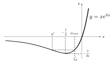
Note that μj(ξ)=ζj(ξ)subscript𝜇𝑗𝜉subscript𝜁𝑗𝜉\mu_{j}(\xi)=\zeta_{j}(\xi) is a trivial solution of (3.9) (see e.g. Fig.7) and there are infinite many μj(ξ)subscript𝜇𝑗𝜉\mu_{j}(\xi) satisfying (3.9) for any given ζj(ξ)subscript𝜁𝑗𝜉\zeta_{j}(\xi). We need μj(ξ)subscript𝜇𝑗𝜉\mu_{j}(\xi) with maximal real parts among them, that is, we take μmax,j(ξ)subscript𝜇𝑚𝑎𝑥𝑗𝜉\mu_{max,j}(\xi) satisfying Re(μmax,j(ξ))=max{Re(μ);μeδμ=ζj(ξ)eδζj(ξ)}𝑅𝑒subscript𝜇𝑚𝑎𝑥𝑗𝜉𝑅𝑒𝜇𝜇superscript𝑒𝛿𝜇subscript𝜁𝑗𝜉superscript𝑒𝛿subscript𝜁𝑗𝜉Re(\mu_{max,j}(\xi))=\displaystyle\max\{Re(\mu);\;\mu e^{\delta\mu}=\zeta_{j}(\xi)e^{\delta\zeta_{j}(\xi)}\}, which is known to be real for ζj(ξ)𝐑subscript𝜁𝑗𝜉𝐑\zeta_{j}(\xi)\in{\bf R} by Proposition2.2. Defining μmax(ξ):=maxj{μmax,j(ξ))}\mu_{max}(\xi):=\displaystyle\max_{j}\{\mu_{max,j}(\xi))\}, we see μmax(ξ)subscript𝜇𝑚𝑎𝑥𝜉\mu_{max}(\xi) is attained by the principal branch of the Lambert W function as μmax(ξ)=1δmaxj{W0(δζj(ξ)eδζj(ξ))}subscript𝜇𝑚𝑎𝑥𝜉1𝛿subscript𝑗subscript𝑊0𝛿subscript𝜁𝑗𝜉superscript𝑒𝛿subscript𝜁𝑗𝜉\mu_{max}(\xi)=\frac{1}{\delta}\cdot\displaystyle\max_{j}\{W_{0}(\delta\zeta_{j}(\xi)e^{\delta\zeta_{j}(\xi)})\} (see Proposition2.2).

Refer to caption
Figure 7: Conceptual figure of solutions μ𝜇\mu of (3.9).

Since μmax(ξ)subscript𝜇𝑚𝑎𝑥𝜉\mu_{max}(\xi) is the most unstable mode, V^(t,ξ)^𝑉𝑡𝜉\widehat{V}(t,\xi) of (3.7) satisfies

|V^(t,ξ)α(ξ)etμmax(ξ)Ψ(ξ)|0(t)^𝑉𝑡𝜉𝛼𝜉superscript𝑒𝑡subscript𝜇𝑚𝑎𝑥𝜉Ψ𝜉0𝑡|\widehat{V}(t,\xi)-\alpha(\xi)e^{t\mu_{max}(\xi)}\Psi(\xi)|\rightarrow 0\;(t\rightarrow\infty) (3.10)

for almost all initial data V^(0,ξ)^𝑉0𝜉\widehat{V}(0,\xi) with some α(ξ)𝛼𝜉\alpha(\xi) and Ψ(ξ)Ψ𝜉\Psi(\xi). When (3.10) holds, it is called that V^(t,ξ)^𝑉𝑡𝜉\widehat{V}(t,\xi) “asymptotically converges” α(ξ)etμmax(ξ)Ψ(ξ)𝛼𝜉superscript𝑒𝑡subscript𝜇𝑚𝑎𝑥𝜉Ψ𝜉\alpha(\xi)e^{t\mu_{max}(\xi)}\Psi(\xi) as t𝑡t\rightarrow\infty. Then we see

U^(t,ξ)=etλh(ξ)V^(t,ξ)α(ξ)et(λh(ξ)+μmax(ξ))Ψ(ξ)^𝑈𝑡𝜉superscript𝑒𝑡subscript𝜆𝜉^𝑉𝑡𝜉𝛼𝜉superscript𝑒𝑡subscript𝜆𝜉subscript𝜇𝑚𝑎𝑥𝜉Ψ𝜉\widehat{U}(t,\xi)=e^{t\lambda_{h}(\xi)}\widehat{V}(t,\xi)\rightarrow\alpha(\xi)e^{t(\lambda_{h}(\xi)+\mu_{max}(\xi))}\Psi(\xi) (3.11)

as t𝑡t\rightarrow\infty. Thus, U^(t)^𝑈𝑡\widehat{U}(t) satisfies asymptotically U^t=(λh(ξ)+μmax(ξ))U^subscript^𝑈𝑡subscript𝜆𝜉subscript𝜇𝑚𝑎𝑥𝜉^𝑈\widehat{U}_{t}=(\lambda_{h}(\xi)+\mu_{max}(\xi))\widehat{U} and therefore for any element of U^^𝑈\widehat{U}, say w^^𝑤\widehat{w}, w^t=(λh(ξ)+μmax(ξ))w^subscript^𝑤𝑡subscript𝜆𝜉subscript𝜇𝑚𝑎𝑥𝜉^𝑤\widehat{w}_{t}=(\lambda_{h}(\xi)+\mu_{max}(\xi))\widehat{w} holds. Since ζj(ξ)0subscript𝜁𝑗𝜉0\zeta_{j}(\xi)\rightarrow 0 or -\infty as |ξ|𝜉|\xi|\rightarrow\infty by the form of Bε(ξ)subscript𝐵𝜀𝜉B_{\varepsilon}(\xi), μmax(ξ)0subscript𝜇𝑚𝑎𝑥𝜉0\mu_{max}(\xi)\rightarrow 0 holds as |ξ|𝜉|\xi|\rightarrow\infty and μmaxL2(𝐑)subscript𝜇𝑚𝑎𝑥superscript𝐿2𝐑\mu_{max}\in L^{2}(\bf R) is expected for almost all cases as shown in several applications mentioned in this paper. Thus we obtain the equation of w𝑤w

wt=d1wxx+Kwsubscript𝑤𝑡subscript𝑑1subscript𝑤𝑥𝑥𝐾𝑤w_{t}=d_{1}w_{xx}+K*w (3.12)

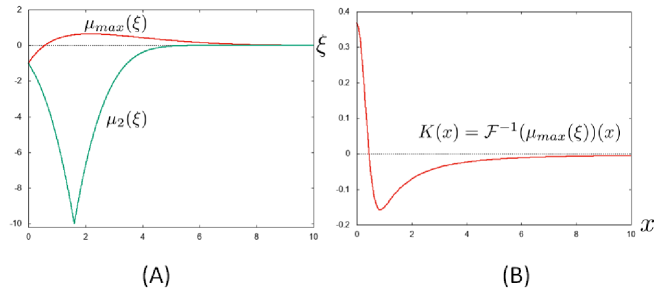
as the effective equation, where we use 1(d1ξ2)=d1x2superscript1subscript𝑑1superscript𝜉2subscript𝑑1superscriptsubscript𝑥2{\cal F}^{-1}(-d_{1}\xi^{2})=d_{1}\partial_{x}^{2} and define K(x):=1(μmax(ξ))(x)assign𝐾𝑥superscript1subscript𝜇𝑚𝑎𝑥𝜉𝑥K(x):={\cal F}^{-1}(\mu_{max}(\xi))(x), the inverse Fourier transformation of the function μmax(ξ)subscript𝜇𝑚𝑎𝑥𝜉\mu_{max}(\xi). Fig.8 is a numerical simulation under the indicated parameters. We note that the kernel K(x)𝐾𝑥K(x) gives the Mexican hat type profile. In practical computations, we use

wt=d1wxx+χ(Kw)subscript𝑤𝑡subscript𝑑1subscript𝑤𝑥𝑥𝜒𝐾𝑤w_{t}=d_{1}w_{xx}+\chi(K*w) (3.13)

with an appropriate cutt-off function χ(r)𝜒𝑟\chi(r) as in (1.4).

Refer to caption
Figure 8: (A) Graph of μmax(ξ)subscript𝜇𝑚𝑎𝑥𝜉\mu_{max}(\xi). μ2(ξ)subscript𝜇2𝜉\mu_{2}(\xi) denotes the second largest Re(μ)𝑅𝑒𝜇Re(\mu) in (3.9). (B) The derived kernel K(x)=(1μmax)(x)𝐾𝑥superscript1subscript𝜇𝑚𝑎𝑥𝑥K(x)=({\cal F}^{-1}\mu_{max})(x). It shows the Mexican hat profile. Parameters are same as those of Fig.6: c1=c2=1subscript𝑐1subscript𝑐21c_{1}=c_{2}=1, c3=4subscript𝑐34c_{3}=4, c4=3subscript𝑐43c_{4}=3, d1=0.05subscript𝑑10.05d_{1}=0.05 and d2=3subscript𝑑23d_{2}=3 in (3.1). ε𝜀\varepsilon and δ𝛿\delta in (3.6) are taken as ε=0.05𝜀0.05\varepsilon=0.05, δ=0.1𝛿0.1\delta=0.1. Only the right half pictures are drawn both in (A) and (B).
Remark 3.1.

The above matrix B(ξ)𝐵𝜉B(\xi) and the eigenvalue λj(ξ)subscript𝜆𝑗𝜉\lambda_{j}(\xi) can be written as B(ξ2)𝐵superscript𝜉2B(\xi^{2}) and λj(ξ2)subscript𝜆𝑗superscript𝜉2\lambda_{j}(\xi^{2}) from the forms. In general, the matrix and the eigenvalue corresponding to B(ξ)𝐵𝜉B(\xi) and λj(ξ)subscript𝜆𝑗𝜉\lambda_{j}(\xi) depend only on ξ2superscript𝜉2\xi^{2} when the spatial movement is only by a local diffusion like this example. In this case, one dimensional analysis is enough because the Fourier transformation on 2D just replaces ξ2superscript𝜉2\xi^{2} by ξ2+η2superscript𝜉2superscript𝜂2\xi^{2}+\eta^{2}, that is, the matrix B(ξ2+η2)𝐵superscript𝜉2superscript𝜂2B(\xi^{2}+\eta^{2}) and the eigenvalue λj(ξ2+η2)subscript𝜆𝑗superscript𝜉2superscript𝜂2\lambda_{j}(\xi^{2}+\eta^{2}) in 2D without any other change, which means the reduced kernel in 1D and 2D are almost same (refer Section 5).

Remark 3.2.

The equations (1.4) and (3.13) seem different each other. But they are essentially same in the following sense: The diffusion is approximated by the relation Jϵu=γ0u+ϵ2γ1uxx+O(ϵ4)subscript𝐽italic-ϵ𝑢subscript𝛾0𝑢superscriptitalic-ϵ2subscript𝛾1subscript𝑢𝑥𝑥𝑂superscriptitalic-ϵ4J_{\epsilon}*u=\gamma_{0}u+\epsilon^{2}\gamma_{1}u_{xx}+O(\epsilon^{4}) as ϵ+0italic-ϵ0\epsilon\rightarrow+0, where Jϵ(x):=1ϵJ(xϵ)assignsubscript𝐽italic-ϵ𝑥1italic-ϵ𝐽𝑥italic-ϵJ_{\epsilon}(x):=\frac{1}{\epsilon}J(\frac{x}{\epsilon}) for an even function J(x)𝐽𝑥J(x) satisfying J(x)0𝐽𝑥0J(x)\geq 0 and γ0:=𝐑J(x)𝑑xassignsubscript𝛾0subscript𝐑𝐽𝑥differential-d𝑥\gamma_{0}:=\displaystyle\int_{\bf R}J(x)dx, γ1:=12𝐑x2J(x)𝑑xassignsubscript𝛾112subscript𝐑superscript𝑥2𝐽𝑥differential-d𝑥\gamma_{1}:=\frac{1}{2}\displaystyle\int_{\bf R}x^{2}J(x)dx (e.g. [3, 13]). Then the reduced equation (3.12) without cut-off function in (3.13) is expressed as

wt=Kwγ0ϵ2γ1w+O(ϵ2)subscript𝑤𝑡superscript𝐾𝑤subscript𝛾0superscriptitalic-ϵ2subscript𝛾1𝑤𝑂superscriptitalic-ϵ2w_{t}=K^{\prime}*w-\frac{\gamma_{0}}{\epsilon^{2}\gamma_{1}}w+O(\epsilon^{2}) (3.14)

with K(x):=d1ϵ2γ1Jϵ(x)+K(x)assignsuperscript𝐾𝑥subscript𝑑1superscriptitalic-ϵ2subscript𝛾1subscript𝐽italic-ϵ𝑥𝐾𝑥K^{\prime}(x):=\frac{d_{1}}{\epsilon^{2}\gamma_{1}}J_{\epsilon}(x)+K(x), which is the same form as (1.4) without cut-off function. Thus, (1.4) and (3.13) are essentially same and we are adopting the equations in the form of (3.13) in this paper.

4 Treatment for arbitrary networks

4.1 Basic treatment for general networks
- case of real eigenvalues -

In this section, we first give the idea to treat general cases of multiple components, but consider on one dimensional space just for the simplicity. Let U=(u1,,uN)t𝐑𝐍U={{}^{t}}(u_{1},\cdots,u_{N})\in\bf R^{N} and U𝑈U is supposed to be described by the equation

Ut=𝐉U+AU,subscript𝑈𝑡𝐉𝑈𝐴𝑈U_{t}={\bf J}U+AU, (4.1)

where 𝐉U:=(J1u1,,JNuN)t{\bf J}U:={{}^{t}}(J_{1}*u_{1},\cdots,J_{N}*u_{N}) for 𝐉:=(J1,,JN)t{\bf J}:={{}^{t}}(J_{1},\cdots,J_{N}) with kernels Jjsubscript𝐽𝑗J_{j} corresponds to the spatial movement and N𝑁N-th order square matrix A𝐴A denotes the local network like the matrix A𝐴A in (3.2). Taking the Fourier transformation of (4.1), we have

U^t=B(ξ)U^,subscript^𝑈𝑡𝐵𝜉^𝑈\widehat{U}_{t}=B(\xi)\widehat{U}, (4.2)

where B(ξ):=𝐉^+Aassign𝐵𝜉^𝐉𝐴B(\xi):=\widehat{\bf J}+A. Let λj(ξ)subscript𝜆𝑗𝜉\lambda_{j}(\xi) (j=1,,N𝑗1𝑁j=1,\cdots,N) be eigenvalues of B(ξ)𝐵𝜉B(\xi). In this subsection, all λj(ξ)subscript𝜆𝑗𝜉\lambda_{j}(\xi) are supposed to be real. Quite similarly to the previous section, we define λmax(ξ):=maxj{λj(ξ)}assignsubscript𝜆𝑚𝑎𝑥𝜉subscript𝑗subscript𝜆𝑗𝜉\lambda_{max}(\xi):=\displaystyle\max_{j}\{\lambda_{j}(\xi)\} and λh(ξ)subscript𝜆𝜉\lambda_{h}(\xi) be the highest order term in ξ𝜉\xi of the asymptotic profile of λmax(ξ)subscript𝜆𝑚𝑎𝑥𝜉\lambda_{max}(\xi) as |ξ|𝜉|\xi|\rightarrow\infty. Here we give the precise way to get λh(ξ)subscript𝜆𝜉\lambda_{h}(\xi). Let λ±(ξ)subscript𝜆plus-or-minus𝜉\lambda_{\pm\infty}(\xi) be the asymptotic profile of λmax(ξ)subscript𝜆𝑚𝑎𝑥𝜉\lambda_{max}(\xi) satisfying λmax(ξ)λ±(ξ)subscript𝜆𝑚𝑎𝑥𝜉subscript𝜆plus-or-minus𝜉\lambda_{max}(\xi)\rightarrow\lambda_{\pm\infty}(\xi) as ξ±𝜉plus-or-minus\xi\rightarrow\pm\infty. When |λ±(ξ)|subscript𝜆plus-or-minus𝜉|\lambda_{\pm\infty}(\xi)|\rightarrow\infty as ξ±𝜉plus-or-minus\xi\rightarrow\pm\infty and the highest order terms of λ±(ξ)subscript𝜆plus-or-minus𝜉\lambda_{\pm\infty}(\xi) are coincident each other, take the same highest order term of λ±(ξ)subscript𝜆plus-or-minus𝜉\lambda_{\pm\infty}(\xi) as λh(ξ)subscript𝜆𝜉\lambda_{h}(\xi) and when λ±(ξ)O(1)subscript𝜆plus-or-minus𝜉𝑂1\lambda_{\pm\infty}(\xi)\rightarrow O(1), take λh(ξ)=0subscript𝜆𝜉0\lambda_{h}(\xi)=0. For example, when λ±(ξ)subscript𝜆plus-or-minus𝜉\lambda_{\pm\infty}(\xi) is given by λ±(ξ)=a1ξ2+a±2ξ+a±3subscript𝜆plus-or-minus𝜉subscript𝑎1superscript𝜉2subscript𝑎plus-or-minus2𝜉subscript𝑎plus-or-minus3\lambda_{\pm\infty}(\xi)=a_{1}\xi^{2}+a_{\pm 2}\xi+a_{\pm 3} for aj𝐂subscript𝑎𝑗𝐂a_{j}\in{\bf C} and a10subscript𝑎10a_{1}\neq 0, we put λh(ξ)=a1ξ2subscript𝜆𝜉subscript𝑎1superscript𝜉2\lambda_{h}(\xi)=a_{1}\xi^{2} and when λ±(ξ)=a±3subscript𝜆plus-or-minus𝜉subscript𝑎plus-or-minus3\lambda_{\pm\infty}(\xi)=a_{\pm 3}, we put λh(ξ)=0subscript𝜆𝜉0\lambda_{h}(\xi)=0.

Transforming U^(t)=etλh(ξ)V^(t)^𝑈𝑡superscript𝑒𝑡subscript𝜆𝜉^𝑉𝑡\widehat{U}(t)=e^{t\lambda_{h}(\xi)}\widehat{V}(t), we have the equation of V^^𝑉\widehat{V}

V^t=Bh(ξ)V^subscript^𝑉𝑡subscript𝐵𝜉^𝑉\widehat{V}_{t}=B_{h}(\xi)\widehat{V} (4.3)

with Bh(ξ):={B(ξ)λh(ξ)I}assignsubscript𝐵𝜉𝐵𝜉subscript𝜆𝜉𝐼B_{h}(\xi):=\{B(\xi)-\lambda_{h}(\xi)I\}. Expressing Bh(ξ)subscript𝐵𝜉B_{h}(\xi) in the form Bh(ξ)=ξB1(ξ)+B0(ξ)subscript𝐵𝜉𝜉subscript𝐵1𝜉subscript𝐵0𝜉B_{h}(\xi)=\xi B_{1}(\xi)+B_{0}(\xi) with B0(ξ)=O(1)subscript𝐵0𝜉𝑂1B_{0}(\xi)=O(1) as |ξ|𝜉|\xi|\rightarrow\infty, we define Bε(ξ):=ξB1(ξ)+eεξ2B0(ξ)assignsubscript𝐵𝜀𝜉𝜉subscript𝐵1𝜉superscript𝑒𝜀superscript𝜉2subscript𝐵0𝜉B_{\varepsilon}(\xi):=\xi B_{1}(\xi)+e^{-\varepsilon\xi^{2}}B_{0}(\xi) and consider the equation

V^t=Bε(ξ)V^subscript^𝑉𝑡subscript𝐵𝜀𝜉^𝑉\widehat{V}_{t}=B_{\varepsilon}(\xi)\widehat{V} (4.4)

instead of (4.3). Let ζj(ξ)subscript𝜁𝑗𝜉\zeta_{j}(\xi) and Φj(ξ)subscriptΦ𝑗𝜉\Phi_{j}(\xi) (j=1,,N𝑗1𝑁j=1,\cdots,N) be eigenvalues and the associated eigenvectors of Bε(ξ)subscript𝐵𝜀𝜉B_{\varepsilon}(\xi), which are supposed to be real in this subsection.

Taking the time t+δ𝑡𝛿t+\delta for 0<δ<<10𝛿much-less-than10<\delta<<1 in (4.4), we see

V^t(t+δ)=Bε(ξ)V^(t+δ)subscript^𝑉𝑡𝑡𝛿subscript𝐵𝜀𝜉^𝑉𝑡𝛿\widehat{V}_{t}(t+\delta)=B_{\varepsilon}(\xi)\widehat{V}(t+\delta) (4.5)

and therefore

V^t(t+δ)=Bε(ξ)eδBε(ξ)V^(t)subscript^𝑉𝑡𝑡𝛿subscript𝐵𝜀𝜉superscript𝑒𝛿subscript𝐵𝜀𝜉^𝑉𝑡\widehat{V}_{t}(t+\delta)=B_{\varepsilon}(\xi)e^{\delta B_{\varepsilon}(\xi)}\widehat{V}(t) (4.6)

from (4.4). Then we express V^(t,ξ)=jαj(ξ)etμj(ξ)Φj(ξ)^𝑉𝑡𝜉subscript𝑗subscript𝛼𝑗𝜉superscript𝑒𝑡subscript𝜇𝑗𝜉subscriptΦ𝑗𝜉\widehat{V}(t,\xi)=\displaystyle\sum_{j}\alpha_{j}(\xi)e^{t\mu_{j}(\xi)}\Phi_{j}(\xi) and the substitution of it into (4.6) leads

μj(ξ)eδμj(ξ)=ζj(ξ)eδζj(ξ)subscript𝜇𝑗𝜉superscript𝑒𝛿subscript𝜇𝑗𝜉subscript𝜁𝑗𝜉superscript𝑒𝛿subscript𝜁𝑗𝜉\mu_{j}(\xi)e^{\delta\mu_{j}(\xi)}=\zeta_{j}(\xi)e^{\delta\zeta_{j}(\xi)} (4.7)

in quite a similar manner to (3.8) and (3.9). Define μmax(ξ)subscript𝜇𝑚𝑎𝑥𝜉\mu_{max}(\xi) as the value satifying

Re(μmax(ξ))=maxj{Re(μ);μeδμ=ζj(ξ)eδζj(ξ),j=1,2,,N}𝑅𝑒subscript𝜇𝑚𝑎𝑥𝜉subscript𝑗𝑅𝑒𝜇𝜇superscript𝑒𝛿𝜇subscript𝜁𝑗𝜉superscript𝑒𝛿subscript𝜁𝑗𝜉𝑗12𝑁Re(\mu_{max}(\xi))=\displaystyle\max_{j}\{Re(\mu);\;\mu e^{\delta\mu}=\zeta_{j}(\xi)e^{\delta\zeta_{j}(\xi)},\;j=1,2,\cdots,N\}

similarly to Section 3, which is given by μmax(ξ)=maxj{1/δW0(δζj(ξ)eδζj(ξ))}subscript𝜇𝑚𝑎𝑥𝜉subscript𝑗1𝛿subscript𝑊0𝛿subscript𝜁𝑗𝜉superscript𝑒𝛿subscript𝜁𝑗𝜉\mu_{max}(\xi)=\displaystyle\max_{j}\{1/\delta\cdot W_{0}(\delta\zeta_{j}(\xi)e^{\delta\zeta_{j}(\xi)})\} when ζj(ξ)𝐑subscript𝜁𝑗𝜉𝐑\zeta_{j}(\xi)\in{\bf R} by Proposition 2.2.

Remark 4.1.

μj(ξ)=ζj(ξ)subscript𝜇𝑗𝜉subscript𝜁𝑗𝜉\mu_{j}(\xi)=\zeta_{j}(\xi) holds when ζj(ξ)>1δsubscript𝜁𝑗𝜉1𝛿\zeta_{j}(\xi)>-\frac{1}{\delta} (see Figure 7).

Since μmax(ξ)subscript𝜇𝑚𝑎𝑥𝜉\mu_{max}(\xi) is the most unstable eigenvalue for ξ𝐑𝜉𝐑\xi\in{\bf R}, we can expect V^(t)^𝑉𝑡\widehat{V}(t) of (4.6) asymptotically converges V^(t,ξ)α(ξ)etμmax(ξ)Φ(ξ)^𝑉𝑡𝜉𝛼𝜉superscript𝑒𝑡subscript𝜇𝑚𝑎𝑥𝜉Φ𝜉\widehat{V}(t,\xi)\rightarrow\alpha(\xi)e^{t\mu_{max}(\xi)}\Phi(\xi) (t𝑡t\rightarrow\infty) with some α(ξ)𝛼𝜉\alpha(\xi) and Φ(ξ)Φ𝜉\Phi(\xi) for almost all initial data and hence

U^(t,ξ)=etλh(ξ)V^(t,ξ)α(ξ)et(λh(ξ)+μmax(ξ))Φ(ξ)^𝑈𝑡𝜉superscript𝑒𝑡subscript𝜆𝜉^𝑉𝑡𝜉𝛼𝜉superscript𝑒𝑡subscript𝜆𝜉subscript𝜇𝑚𝑎𝑥𝜉Φ𝜉\widehat{U}(t,\xi)=e^{t\lambda_{h}(\xi)}\widehat{V}(t,\xi)\rightarrow\alpha(\xi)e^{t(\lambda_{h}(\xi)+\mu_{max}(\xi))}\Phi(\xi) (4.8)

as t𝑡t\rightarrow\infty. Thus, U^(t)^𝑈𝑡\widehat{U}(t) satisfies asymptotically U^t=(λh(ξ)+μmax(ξ))U^subscript^𝑈𝑡subscript𝜆𝜉subscript𝜇𝑚𝑎𝑥𝜉^𝑈\widehat{U}_{t}=(\lambda_{h}(\xi)+\mu_{max}(\xi))\widehat{U} and therefore for any element of U^^𝑈\widehat{U}, say w^^𝑤\widehat{w}, w^t=(λh(ξ)+μmax(ξ))w^subscript^𝑤𝑡subscript𝜆𝜉subscript𝜇𝑚𝑎𝑥𝜉^𝑤\widehat{w}_{t}=(\lambda_{h}(\xi)+\mu_{max}(\xi))\widehat{w} holds. Consequently we obtain the equation of w𝑤w

wt=w+Kwsubscript𝑤𝑡𝑤𝐾𝑤w_{t}={\cal L}w+K*w (4.9)

as the effective equation, where K(x):=1(μmax(ξ))assign𝐾𝑥superscript1subscript𝜇𝑚𝑎𝑥𝜉K(x):={\cal F}^{-1}(\mu_{max}(\xi)) and :=1(λh(ξ))assignsuperscript1subscript𝜆𝜉{\cal L}:={\cal F}^{-1}(\lambda_{h}(\xi)), which is treated as a differential operator such as 1(ξ2)=x2superscript1superscript𝜉2superscriptsubscript𝑥2{\cal F}^{-1}(-\xi^{2})=\partial_{x}^{2}. Here we note that μmax(ξ)0subscript𝜇𝑚𝑎𝑥𝜉0\mu_{max}(\xi)\rightarrow 0 as |ξ|𝜉|\xi|\rightarrow\infty because ζj(ξ)0subscript𝜁𝑗𝜉0\zeta_{j}(\xi)\rightarrow 0 or -\infty.

This is the basic idea in the case that all λj(ξ)subscript𝜆𝑗𝜉\lambda_{j}(\xi) are real valued and there exists only one maximal eigenvalue for each ξ𝜉\xi. But this is a specially simple case because there can be several other cases. In the following subsection, the case that B(ξ)𝐵𝜉B(\xi) have complex eigenvalues on some range of ξ𝐑𝜉𝐑\xi\in{\bf R} is considered.

4.2 Basic treatment for general networks
- case of complex eigenvalues -

In this section, we consider the case that B(ξ)𝐵𝜉B(\xi) in (4.2) have complex eigenvalues for an interval of ξ𝜉\xi. We define λmax(ξ):=maxj{Re(λj(ξ))}assignsubscript𝜆𝑚𝑎𝑥𝜉subscript𝑗𝑅𝑒subscript𝜆𝑗𝜉\lambda_{max}(\xi):=\displaystyle\max_{j}\{Re(\lambda_{j}(\xi))\} and the asymptotic profile λ(ξ)subscript𝜆𝜉\lambda_{\infty}(\xi) of λmax(ξ)subscript𝜆𝑚𝑎𝑥𝜉\lambda_{max}(\xi) by λmax(ξ)λ(ξ)subscript𝜆𝑚𝑎𝑥𝜉subscript𝜆𝜉\lambda_{max}(\xi)\rightarrow\lambda_{\infty}(\xi) as |ξ|𝜉|\xi|\rightarrow\infty. First, we assume

λj(ξ)λ(ξ)0(|ξ|).subscript𝜆𝑗𝜉subscript𝜆𝜉0𝜉\lambda_{j}(\xi)-\lambda_{\infty}(\xi)\rightarrow 0\;(|\xi|\rightarrow\infty). (4.10)

Let λh(ξ)subscript𝜆𝜉\lambda_{h}(\xi) be the highest order term of λ(ξ)subscript𝜆𝜉\lambda_{\infty}(\xi) and Bh(ξ):=B(ξ)λh(ξ)Iassignsubscript𝐵𝜉𝐵𝜉subscript𝜆𝜉𝐼B_{h}(\xi):=B(\xi)-\lambda_{h}(\xi)I. As in the previous section, we divide Bh(ξ)subscript𝐵𝜉B_{h}(\xi) as Bh(ξ)=ξB1(ξ)+B0(ξ)subscript𝐵𝜉𝜉subscript𝐵1𝜉subscript𝐵0𝜉B_{h}(\xi)=\xi B_{1}(\xi)+B_{0}(\xi) with B0(ξ)=O(1)subscript𝐵0𝜉𝑂1B_{0}(\xi)=O(1) and define Bε(ξ)=ξB1(ξ)+eεξ2B0(ξ)subscript𝐵𝜀𝜉𝜉subscript𝐵1𝜉superscript𝑒𝜀superscript𝜉2subscript𝐵0𝜉B_{\varepsilon}(\xi)=\xi B_{1}(\xi)+e^{-\varepsilon\xi^{2}}B_{0}(\xi).

Let ζj(ξ)subscript𝜁𝑗𝜉\zeta_{j}(\xi) and Φj(ξ)subscriptΦ𝑗𝜉\Phi_{j}(\xi) be eigenvalues and the associated eigenvectors of Bε(ξ)subscript𝐵𝜀𝜉B_{\varepsilon}(\xi) and consider the equation (4.6) together with (4.7) in the case of complex eigenvalues. Define

μmax(ξ):=maxj{Re(μ);μeδμ=ζj(ξ)eδζj(ξ),j=1,2,,N}assignsubscript𝜇𝑚𝑎𝑥𝜉subscript𝑗𝑅𝑒𝜇𝜇superscript𝑒𝛿𝜇subscript𝜁𝑗𝜉superscript𝑒𝛿subscript𝜁𝑗𝜉𝑗12𝑁\mu_{max}(\xi):=\displaystyle\max_{j}\{Re(\mu);\;\mu e^{\delta\mu}=\zeta_{j}(\xi)e^{\delta\zeta_{j}(\xi)},\;j=1,2,\cdots,N\}

and assume that ζ1(ξ)subscript𝜁1𝜉\zeta_{1}(\xi), ζ2(ξ)subscript𝜁2𝜉\zeta_{2}(\xi) satisfy the following three assumptions (H1), (H2) and (H3).

(H1): μmax(ξ)subscript𝜇𝑚𝑎𝑥𝜉\mu_{max}(\xi) is attained by ζ1(ξ)subscript𝜁1𝜉\zeta_{1}(\xi), that is, μmax(ξ)=max{Re(μ);μeδμ=ζ1(ξ)eδζ1(ξ)}subscript𝜇𝑚𝑎𝑥𝜉𝑅𝑒𝜇𝜇superscript𝑒𝛿𝜇subscript𝜁1𝜉superscript𝑒𝛿subscript𝜁1𝜉\mu_{max}(\xi)=\max\{Re(\mu);\;\mu e^{\delta\mu}=\zeta_{1}(\xi)e^{\delta\zeta_{1}(\xi)}\}.
(H2): There exists ξcsubscript𝜉𝑐\xi_{c} such that ζ1(ξ)>ζ2(ξ)subscript𝜁1𝜉subscript𝜁2𝜉\zeta_{1}(\xi)>\zeta_{2}(\xi) for ξ<ξc𝜉subscript𝜉𝑐\xi<\xi_{c}, ζ1(ξc)=ζ2(ξc)𝐑subscript𝜁1subscript𝜉𝑐subscript𝜁2subscript𝜉𝑐𝐑\zeta_{1}(\xi_{c})=\zeta_{2}(\xi_{c})\in{\bf R} and ζ1(ξ)=ζ2(ξ)¯=a(ξ)+ib(ξ)subscript𝜁1𝜉¯subscript𝜁2𝜉𝑎𝜉𝑖𝑏𝜉\zeta_{1}(\xi)=\overline{\zeta_{2}(\xi)}=a(\xi)+ib(\xi)for ξ>ξc𝜉subscript𝜉𝑐\xi>\xi_{c} with a(ξ)𝐑𝑎𝜉𝐑a(\xi)\in{\bf R} and b(ξ)>0𝑏𝜉0b(\xi)>0 satisfying a(ξc)=ζ1(ξc)=ζ2(ξc)𝑎subscript𝜉𝑐subscript𝜁1subscript𝜉𝑐subscript𝜁2subscript𝜉𝑐a(\xi_{c})=\zeta_{1}(\xi_{c})=\zeta_{2}(\xi_{c}) and b(ξc)=0𝑏subscript𝜉𝑐0b(\xi_{c})=0. Moreover, Φ1(ξc)=Φ2(ξc)subscriptΦ1subscript𝜉𝑐subscriptΦ2subscript𝜉𝑐\Phi_{1}(\xi_{c})=\Phi_{2}(\xi_{c}) holds.
(H3): Define Ψ(ξ):=Φ2(ξ)Φ1(ξ)ζ2(ξ)ζ1(ξ)assignΨ𝜉subscriptΦ2𝜉subscriptΦ1𝜉subscript𝜁2𝜉subscript𝜁1𝜉\Psi(\xi):=\displaystyle\frac{\Phi_{2}(\xi)-\Phi_{1}(\xi)}{\zeta_{2}(\xi)-\zeta_{1}(\xi)}. Then, there exists a limit limξξcΨ(ξ)subscript𝜉subscript𝜉𝑐Ψ𝜉\displaystyle\lim_{\xi\rightarrow\xi_{c}}\Psi(\xi).

Remark 4.2.

It follows that b(ξ)0𝑏𝜉0b(\xi)\rightarrow 0 as |ξ|𝜉|\xi|\rightarrow\infty by (4.10) and also that Ψ(ξ)Ψ𝜉\Psi(\xi) is a continuous real vector-valued function on the whole line 𝐑𝐑{\bf R} by the definition in (H3).

Substituting Φ2(ξ)=Φ1(ξ)+{ζ2(ξ)ζ1(ξ)}Ψ(ξ)subscriptΦ2𝜉subscriptΦ1𝜉subscript𝜁2𝜉subscript𝜁1𝜉Ψ𝜉\Phi_{2}(\xi)=\Phi_{1}(\xi)+\{\zeta_{2}(\xi)-\zeta_{1}(\xi)\}\Psi(\xi) into Bε(ξ)Φ2(ξ)=ζ2(ξ)Φ2(ξ)subscript𝐵𝜀𝜉subscriptΦ2𝜉subscript𝜁2𝜉subscriptΦ2𝜉B_{\varepsilon}(\xi)\Phi_{2}(\xi)=\zeta_{2}(\xi)\Phi_{2}(\xi) for ξ<ξc𝜉subscript𝜉𝑐\xi<\xi_{c}, we have ζ1(ξ)Φ1(ξ)+{ζ2(ξ)ζ1(ξ)}Bε(ξ)Ψ(ξ)=ζ2(ξ)Φ1(ξ)+ζ2(ξ){ζ2(ξ)ζ1(ξ)}Bε(ξ)Ψ(ξ)subscript𝜁1𝜉subscriptΦ1𝜉subscript𝜁2𝜉subscript𝜁1𝜉subscript𝐵𝜀𝜉Ψ𝜉subscript𝜁2𝜉subscriptΦ1𝜉subscript𝜁2𝜉subscript𝜁2𝜉subscript𝜁1𝜉subscript𝐵𝜀𝜉Ψ𝜉\zeta_{1}(\xi)\Phi_{1}(\xi)+\{\zeta_{2}(\xi)-\zeta_{1}(\xi)\}B_{\varepsilon}(\xi)\Psi(\xi)=\zeta_{2}(\xi)\Phi_{1}(\xi)+\zeta_{2}(\xi)\{\zeta_{2}(\xi)-\zeta_{1}(\xi)\}B_{\varepsilon}(\xi)\Psi(\xi) and consequently {Bε(ξ)ζ2(ξ)I}Φ~(ξ)=Φ1(ξ)subscript𝐵𝜀𝜉subscript𝜁2𝜉𝐼~Φ𝜉subscriptΦ1𝜉\{B_{\varepsilon}(\xi)-\zeta_{2}(\xi)I\}\widetilde{\Phi}(\xi)=\Phi_{1}(\xi). That is,

{{Bε(ξ)ζ1(ξ)I}Φ1(ξ)=0,{Bε(ξ)ζ2(ξ)I}Ψ(ξ)=Φ1(ξ)casessubscript𝐵𝜀𝜉subscript𝜁1𝜉𝐼subscriptΦ1𝜉0subscript𝐵𝜀𝜉subscript𝜁2𝜉𝐼Ψ𝜉subscriptΦ1𝜉\left\{\begin{array}[]{lcl}\{B_{\varepsilon}(\xi)-\zeta_{1}(\xi)I\}\Phi_{1}(\xi)&=&0,\\ \{B_{\varepsilon}(\xi)-\zeta_{2}(\xi)I\}\Psi(\xi)&=&\Phi_{1}(\xi)\end{array}\right. (4.11)

holds for ξ<ξc𝜉subscript𝜉𝑐\xi<\xi_{c}.

On the other hand, we have for ξ>ξc𝜉subscript𝜉𝑐\xi>\xi_{c},

{{Bε(ξ)a(ξ)I}𝐩(ξ)=b(ξ)𝐪(ξ),{Bε(ξ)a(ξ)I}𝐪(ξ)=b(ξ)𝐩(ξ)casessubscript𝐵𝜀𝜉𝑎𝜉𝐼𝐩𝜉𝑏𝜉𝐪𝜉subscript𝐵𝜀𝜉𝑎𝜉𝐼𝐪𝜉𝑏𝜉𝐩𝜉\left\{\begin{array}[]{lcl}\{B_{\varepsilon}(\xi)-a(\xi)I\}{\bf p}(\xi)&=&-b(\xi){\bf q}(\xi),\\ \{B_{\varepsilon}(\xi)-a(\xi)I\}{\bf q}(\xi)&=&b(\xi){\bf p}(\xi)\end{array}\right.

when we express Φ1(ξ)=𝐩(ξ)+i𝐪(ξ)=Φ2(ξ)¯subscriptΦ1𝜉𝐩𝜉𝑖𝐪𝜉¯subscriptΦ2𝜉\Phi_{1}(\xi)={\bf p}(\xi)+i{\bf q}(\xi)=\overline{\Phi_{2}(\xi)} with 𝐩(ξ),𝐪(ξ)𝐑N𝐩𝜉𝐪𝜉superscript𝐑𝑁{\bf p}(\xi),\;{\bf q}(\xi)\in{\bf R}^{N}. Since the definition of Ψ(ξ)Ψ𝜉\Psi(\xi) leads 𝐪(ξ)=b(ξ)Ψ(ξ)𝐪𝜉𝑏𝜉Ψ𝜉{\bf q}(\xi)=b(\xi)\Psi(\xi) and consequently

{{Bε(ξ)a(ξ)I}𝐩(ξ)=b2(ξ)Ψ(ξ),{Bε(ξ)a(ξ)I}Ψ(ξ)=𝐩(ξ)casessubscript𝐵𝜀𝜉𝑎𝜉𝐼𝐩𝜉superscript𝑏2𝜉Ψ𝜉subscript𝐵𝜀𝜉𝑎𝜉𝐼Ψ𝜉𝐩𝜉\left\{\begin{array}[]{lcl}\{B_{\varepsilon}(\xi)-a(\xi)I\}{\bf p}(\xi)&=&-b^{2}(\xi)\Psi(\xi),\\ \{B_{\varepsilon}(\xi)-a(\xi)I\}\Psi(\xi)&=&{\bf p}(\xi)\end{array}\right. (4.12)

for ξ>ξc𝜉subscript𝜉𝑐\xi>\xi_{c}. (4.11) and (4.12) imply that the functions b(ξ)𝑏𝜉b(\xi), ζj(ξ)subscript𝜁𝑗𝜉\zeta_{j}(\xi) (j=1,2𝑗12j=1,2) and the vector Φ1(ξ)subscriptΦ1𝜉\Phi_{1}(\xi) can be extended as real valued continuous functions and a vector on the whole line 𝐑𝐑{\bf R} by

b(ξ):={0(ξξc)b(ξ)(ξ>ξc),ωj(ξ):={ζj(ξ)(ξξc)a(ξ)(ξ>ξc),Ψ1(ξ):={Φ1(ξ)(ξξc)𝐩(ξ)(ξ>ξc).formulae-sequenceassign𝑏𝜉cases0𝜉subscript𝜉𝑐𝑏𝜉𝜉subscript𝜉𝑐formulae-sequenceassignsubscript𝜔𝑗𝜉casessubscript𝜁𝑗𝜉𝜉subscript𝜉𝑐𝑎𝜉𝜉subscript𝜉𝑐assignsubscriptΨ1𝜉casessubscriptΦ1𝜉𝜉subscript𝜉𝑐𝐩𝜉𝜉subscript𝜉𝑐b(\xi):=\left\{\begin{array}[]{cc}0&(\xi\leq\xi_{c})\\ b(\xi)&(\xi>\xi_{c})\end{array}\right.,\;\omega_{j}(\xi):=\left\{\begin{array}[]{cc}\zeta_{j}(\xi)&(\xi\leq\xi_{c})\\ a(\xi)&(\xi>\xi_{c})\end{array}\right.,\;\Psi_{1}(\xi):=\left\{\begin{array}[]{cc}\Phi_{1}(\xi)&(\xi\leq\xi_{c})\\ {\bf p}(\xi)&(\xi>\xi_{c})\end{array}\right.. (4.13)

Thus (4.11) and (4.12) are unified as one system on 𝐑𝐑{\bf R}

{{Bε(ξ)ω1(ξ)I}Ψ1(ξ)=b2(ξ)Ψ,{Bε(ξ)ω2(ξ)I}Ψ(ξ)=Ψ1(ξ).casessubscript𝐵𝜀𝜉subscript𝜔1𝜉𝐼subscriptΨ1𝜉superscript𝑏2𝜉Ψsubscript𝐵𝜀𝜉subscript𝜔2𝜉𝐼Ψ𝜉subscriptΨ1𝜉\left\{\begin{array}[]{lcl}\{B_{\varepsilon}(\xi)-\omega_{1}(\xi)I\}\Psi_{1}(\xi)&=&-b^{2}(\xi)\Psi,\\ \{B_{\varepsilon}(\xi)-\omega_{2}(\xi)I\}\Psi(\xi)&=&\Psi_{1}(\xi).\end{array}\right. (4.14)

Now we go back the equation (4.6) of V^^𝑉\widehat{V}. Let the solution V^^𝑉\widehat{V} of (4.6) be of the form αΨ1(ξ)+βΨ(ξ)𝛼subscriptΨ1𝜉𝛽Ψ𝜉\alpha\Psi_{1}(\xi)+\beta\Psi(\xi) for α,β𝐑𝛼𝛽𝐑\alpha,\;\beta\in{\bf R}. Since (4.14) shows

Bε(ξ)(αΨ1(ξ)+βΨ(ξ))=(ω1(ξ)α+β)Ψ1(ξ)+(b2(ξ)α+ω2(ξ)β)Ψ(ξ),subscript𝐵𝜀𝜉𝛼subscriptΨ1𝜉𝛽Ψ𝜉subscript𝜔1𝜉𝛼𝛽subscriptΨ1𝜉superscript𝑏2𝜉𝛼subscript𝜔2𝜉𝛽Ψ𝜉B_{\varepsilon}(\xi)(\alpha\Psi_{1}(\xi)+\beta\Psi(\xi))=(\omega_{1}(\xi)\alpha+\beta)\Psi_{1}(\xi)+(-b^{2}(\xi)\alpha+\omega_{2}(\xi)\beta)\Psi(\xi),

(4.6) becomes the equation of α𝛼\alpha and β𝛽\beta as

ddt(α(t+δ)β(t+δ))=B~ε(ξ)eδB~ε(ξ)(α(t)β(t)),𝑑𝑑𝑡𝛼𝑡𝛿𝛽𝑡𝛿subscript~𝐵𝜀𝜉superscript𝑒𝛿subscript~𝐵𝜀𝜉𝛼𝑡𝛽𝑡\displaystyle\frac{d}{dt}\left(\begin{array}[]{c}\alpha(t+\delta)\\ \beta(t+\delta)\end{array}\right)=\widetilde{B}_{\varepsilon}(\xi)e^{\delta\widetilde{B}_{\varepsilon}(\xi)}\left(\begin{array}[]{c}\alpha(t)\\ \beta(t)\end{array}\right), (4.15)

where B~ε(ξ):=(ω1(ξ)1b2(ξ)ω2(ξ))assignsubscript~𝐵𝜀𝜉subscript𝜔1𝜉1superscript𝑏2𝜉subscript𝜔2𝜉\widetilde{B}_{\varepsilon}(\xi):=\left(\begin{array}[]{cc}\omega_{1}(\xi)&1\\ -b^{2}(\xi)&\omega_{2}(\xi)\end{array}\right). Since the eigenvalues of B~ε(ξ)subscript~𝐵𝜀𝜉\widetilde{B}_{\varepsilon}(\xi) are ω~1(ξ):=ω1(ξ)+ib(ξ)assignsubscript~𝜔1𝜉subscript𝜔1𝜉𝑖𝑏𝜉\widetilde{\omega}_{1}(\xi):=\omega_{1}(\xi)+ib(\xi) and ω~2(ξ):=ω2(ξ)ib(ξ)assignsubscript~𝜔2𝜉subscript𝜔2𝜉𝑖𝑏𝜉\widetilde{\omega}_{2}(\xi):=\omega_{2}(\xi)-ib(\xi) with associated eigenvectors Ψ~1(ξ)=(1,ib(ξ))t\widetilde{\Psi}_{1}(\xi)={{}^{t}}(1,ib(\xi)) and Ψ~2(ξ)=(1,ω2(ξ)ω1(ξ)ib(ξ))t\widetilde{\Psi}_{2}(\xi)={{}^{t}}(1,\omega_{2}(\xi)-\omega_{1}(\xi)-ib(\xi)) respectively, (αβ)=etμΨ~𝛼𝛽superscript𝑒𝑡𝜇~Ψ\left(\begin{array}[]{c}\alpha\\ \beta\end{array}\right)=e^{t\mu}\widetilde{\Psi} with (4.15) leads

μeδμ=ω~jeδω~j=eδωj{(ωjcosδbbsinδb)±i(bcosδb+ωjsinδb)}𝜇superscript𝑒𝛿𝜇subscript~𝜔𝑗superscript𝑒𝛿subscript~𝜔𝑗superscript𝑒𝛿subscript𝜔𝑗plus-or-minussubscript𝜔𝑗𝛿𝑏𝑏𝛿𝑏𝑖𝑏𝛿𝑏subscript𝜔𝑗𝛿𝑏\mu e^{\delta\mu}=\widetilde{\omega}_{j}e^{\delta\widetilde{\omega}_{j}}=e^{\delta\omega_{j}}\{(\omega_{j}\cos\delta b-b\sin\delta b)\pm i(b\cos\delta b+\omega_{j}\sin\delta b)\} (4.16)

by taking Ψ~=Ψ~j(ξ)~Ψsubscript~Ψ𝑗𝜉\widetilde{\Psi}=\widetilde{\Psi}_{j}(\xi). Let the set ~j(ξ):={μ;μeδμ=ω~jeδω~j}assignsubscript~𝑗𝜉𝜇𝜇superscript𝑒𝛿𝜇subscript~𝜔𝑗superscript𝑒𝛿subscript~𝜔𝑗\widetilde{{\cal M}}_{j}(\xi):=\{\mu;\;\mu e^{\delta\mu}=\widetilde{\omega}_{j}e^{\delta\widetilde{\omega}_{j}}\} and define μ~j(ξ)~j(ξ)subscript~𝜇𝑗𝜉subscript~𝑗𝜉\widetilde{\mu}_{j}(\xi)\in\widetilde{{\cal M}}_{j}(\xi) for j=1,2𝑗12j=1,2 such that Re(μ~j(ξ))=max{Re(μ);μ~j(ξ)}𝑅𝑒subscript~𝜇𝑗𝜉𝑅𝑒𝜇𝜇subscript~𝑗𝜉Re(\widetilde{\mu}_{j}(\xi))=\max\{Re(\mu);\;\mu\in\widetilde{{\cal M}}_{j}(\xi)\}. Here we note that these μ~j(ξ)subscript~𝜇𝑗𝜉\widetilde{\mu}_{j}(\xi) give μmax(ξ)subscript𝜇𝑚𝑎𝑥𝜉\mu_{max}(\xi), that is, μmax(ξ)=maxj=1,2{Re(μ~j(ξ))}subscript𝜇𝑚𝑎𝑥𝜉subscript𝑗12𝑅𝑒subscript~𝜇𝑗𝜉\mu_{max}(\xi)=\displaystyle\max_{j=1,2}\{Re(\widetilde{\mu}_{j}(\xi))\}. Then we can take the solution (αβ)𝛼𝛽\left(\begin{array}[]{c}\alpha\\ \beta\end{array}\right) of (4.15) by (α(t)β(t))=etμ~1Ψ~1+etμ~2Ψ~2𝛼𝑡𝛽𝑡superscript𝑒𝑡subscript~𝜇1subscript~Ψ1superscript𝑒𝑡subscript~𝜇2subscript~Ψ2\left(\begin{array}[]{c}\alpha(t)\\ \beta(t)\end{array}\right)=e^{t\widetilde{\mu}_{1}}\widetilde{\Psi}_{1}+e^{t\widetilde{\mu}_{2}}\widetilde{\Psi}_{2}, which leads the equation of α(t)𝛼𝑡\alpha(t) and β(t)𝛽𝑡\beta(t) as

ddt(αβ)𝑑𝑑𝑡𝛼𝛽\displaystyle\displaystyle\frac{d}{dt}\left(\begin{array}[]{c}\alpha\\ \beta\end{array}\right) =\displaystyle= [Ψ~1,Ψ~2](μ~100μ~2)[Ψ~1,Ψ~2]1(αβ)subscript~Ψ1subscript~Ψ2subscript~𝜇100subscript~𝜇2superscriptsubscript~Ψ1subscript~Ψ21𝛼𝛽\displaystyle[\widetilde{\Psi}_{1},\widetilde{\Psi}_{2}]\left(\begin{array}[]{cc}\widetilde{\mu}_{1}&0\\ 0&\widetilde{\mu}_{2}\end{array}\right)[\widetilde{\Psi}_{1},\widetilde{\Psi}_{2}]^{-1}\left(\begin{array}[]{c}\alpha\\ \beta\end{array}\right) (4.23)
=\displaystyle= 1ω2ω12ib((ω2ω1)μ~1ib(μ~1+μ~2)μ~1+μ~2ib(ω2ω1ib)(μ~1μ~2)(ω2ω1)μ~2ib(μ~1+μ~2))(αβ).1subscript𝜔2subscript𝜔12𝑖𝑏subscript𝜔2subscript𝜔1subscript~𝜇1𝑖𝑏subscript~𝜇1subscript~𝜇2subscript~𝜇1subscript~𝜇2𝑖𝑏subscript𝜔2subscript𝜔1𝑖𝑏subscript~𝜇1subscript~𝜇2subscript𝜔2subscript𝜔1subscript~𝜇2𝑖𝑏subscript~𝜇1subscript~𝜇2𝛼𝛽\displaystyle\displaystyle\frac{1}{\omega_{2}-\omega_{1}-2ib}\left(\begin{array}[]{cc}(\omega_{2}-\omega_{1})\widetilde{\mu}_{1}-ib(\widetilde{\mu}_{1}+\widetilde{\mu}_{2})&-\widetilde{\mu}_{1}+\widetilde{\mu}_{2}\\ ib(\omega_{2}-\omega_{1}-ib)(\widetilde{\mu}_{1}-\widetilde{\mu}_{2})&(\omega_{2}-\omega_{1})\widetilde{\mu}_{2}-ib(\widetilde{\mu}_{1}+\widetilde{\mu}_{2})\end{array}\right)\left(\begin{array}[]{c}\alpha\\ \beta\end{array}\right). (4.28)

By the way of construction in (4.13), we see ω~1(ξ)ω~2(ξ)subscript~𝜔1𝜉subscript~𝜔2𝜉\widetilde{\omega}_{1}(\xi)\neq\widetilde{\omega}_{2}(\xi) and ω~j(ξ)=ζj(ξ)𝐑subscript~𝜔𝑗𝜉subscript𝜁𝑗𝜉𝐑\widetilde{\omega}_{j}(\xi)=\zeta_{j}(\xi)\in{\bf R} for ξ<ξc𝜉subscript𝜉𝑐\xi<\xi_{c}, ω~1(ξc)=ω~2(ξc)subscript~𝜔1subscript𝜉𝑐subscript~𝜔2subscript𝜉𝑐\widetilde{\omega}_{1}(\xi_{c})=\widetilde{\omega}_{2}(\xi_{c}), ω~1(ξ)=ω~2(ξ)¯subscript~𝜔1𝜉¯subscript~𝜔2𝜉\widetilde{\omega}_{1}(\xi)=\overline{\widetilde{\omega}_{2}(\xi)} for ξ>ξc𝜉subscript𝜉𝑐\xi>\xi_{c}, we can also assume μ~1(ξ)μ~2(ξ)subscript~𝜇1𝜉subscript~𝜇2𝜉\widetilde{\mu}_{1}(\xi)\neq\widetilde{\mu}_{2}(\xi) and μ~j(ξ)𝐑subscript~𝜇𝑗𝜉𝐑\widetilde{\mu}_{j}(\xi)\in{\bf R} for ξ<ξc𝜉subscript𝜉𝑐\xi<\xi_{c}, μ~1(ξc)=μ~2(ξc)subscript~𝜇1subscript𝜉𝑐subscript~𝜇2subscript𝜉𝑐\widetilde{\mu}_{1}(\xi_{c})=\widetilde{\mu}_{2}(\xi_{c}), μ~1(ξ)=μ~2(ξ)¯subscript~𝜇1𝜉¯subscript~𝜇2𝜉\widetilde{\mu}_{1}(\xi)=\overline{\widetilde{\mu}_{2}(\xi)} for ξ>ξc𝜉subscript𝜉𝑐\xi>\xi_{c}. Then, (4.23) becomes

ddt(αβ)=1ζ2ζ1((ζ2ζ1)μ~1μ~1+μ~20(ζ2ζ1)μ~2)(αβ)=(μ~1μ~2μ~1ω2ω10μ~2)(αβ)𝑑𝑑𝑡𝛼𝛽1subscript𝜁2subscript𝜁1subscript𝜁2subscript𝜁1subscript~𝜇1subscript~𝜇1subscript~𝜇20subscript𝜁2subscript𝜁1subscript~𝜇2𝛼𝛽subscript~𝜇1subscript~𝜇2subscript~𝜇1subscript𝜔2subscript𝜔10subscript~𝜇2𝛼𝛽\displaystyle\frac{d}{dt}\left(\begin{array}[]{c}\alpha\\ \beta\end{array}\right)=\displaystyle\frac{1}{\zeta_{2}-\zeta_{1}}\left(\begin{array}[]{cc}(\zeta_{2}-\zeta_{1})\widetilde{\mu}_{1}&-\widetilde{\mu}_{1}+\widetilde{\mu}_{2}\\ 0&(\zeta_{2}-\zeta_{1})\widetilde{\mu}_{2}\end{array}\right)\left(\begin{array}[]{c}\alpha\\ \beta\end{array}\right)=\left(\begin{array}[]{cc}\widetilde{\mu}_{1}&\frac{\widetilde{\mu}_{2}-\widetilde{\mu}_{1}}{\omega_{2}-\omega_{1}}\\ 0&\widetilde{\mu}_{2}\end{array}\right)\left(\begin{array}[]{c}\alpha\\ \beta\end{array}\right) (4.29)

for ξ<ξc𝜉subscript𝜉𝑐\xi<\xi_{c} and

ddt(αβ)=12ib(ib(μ~1+μ~2)μ~1+μ~2b2(μ~1μ~2)ib(μ~1+μ~2))(αβ)=(a~b~/bb~ba~)(αβ)𝑑𝑑𝑡𝛼𝛽12𝑖𝑏𝑖𝑏subscript~𝜇1subscript~𝜇2subscript~𝜇1subscript~𝜇2superscript𝑏2subscript~𝜇1subscript~𝜇2𝑖𝑏subscript~𝜇1subscript~𝜇2𝛼𝛽~𝑎~𝑏𝑏~𝑏𝑏~𝑎𝛼𝛽\displaystyle\frac{d}{dt}\left(\begin{array}[]{c}\alpha\\ \beta\end{array}\right)=\displaystyle\frac{1}{-2ib}\left(\begin{array}[]{cc}-ib(\widetilde{\mu}_{1}+\widetilde{\mu}_{2})&-\widetilde{\mu}_{1}+\widetilde{\mu}_{2}\\ b^{2}(\widetilde{\mu}_{1}-\widetilde{\mu}_{2})&-ib(\widetilde{\mu}_{1}+\widetilde{\mu}_{2})\end{array}\right)\left(\begin{array}[]{c}\alpha\\ \beta\end{array}\right)=\left(\begin{array}[]{cc}\widetilde{a}&\widetilde{b}/b\\ -\widetilde{b}b&\widetilde{a}\end{array}\right)\left(\begin{array}[]{c}\alpha\\ \beta\end{array}\right) (4.30)

for ξ>ξc𝜉subscript𝜉𝑐\xi>\xi_{c}, where μ~1(ξ)=μ~2(ξ)¯=a~(ξ)+ib~(ξ)subscript~𝜇1𝜉¯subscript~𝜇2𝜉~𝑎𝜉𝑖~𝑏𝜉\widetilde{\mu}_{1}(\xi)=\overline{\widetilde{\mu}_{2}(\xi)}=\widetilde{a}(\xi)+i\widetilde{b}(\xi) for ξ>ξc𝜉subscript𝜉𝑐\xi>\xi_{c}. Therefore, if the limit exists and

limξξc0μ~2(ξ)μ~1(ξ)ζ2(ξ)ζ1(ξ)=limξξc+0b~(ξ)b(ξ)=:p~c\displaystyle\lim_{\xi\rightarrow\xi_{c}-0}\frac{\widetilde{\mu}_{2}(\xi)-\widetilde{\mu}_{1}(\xi)}{\zeta_{2}(\xi)-\zeta_{1}(\xi)}=\displaystyle\lim_{\xi\rightarrow\xi_{c}+0}\frac{\widetilde{b}(\xi)}{b(\xi)}=:\widetilde{p}_{c}

holds, then we can define real valued continuous functions on 𝐑𝐑{\bf R} by

p~(ξ):={μ~2(ξ)μ~1(ξ)ζ2(ξ)ζ1(ξ)(ξ<ξc)p~c(ξ=ξc)b~(ξ)b(ξ)(ξ>ξc),ν~j(ξ):={μ~j(ξ)(ξξc)a~(ξ)(ξ>ξc),q~(ξ):={0(ξξc)b~(ξ)b(ξ)(ξ>ξc)formulae-sequenceassign~𝑝𝜉casessubscript~𝜇2𝜉subscript~𝜇1𝜉subscript𝜁2𝜉subscript𝜁1𝜉𝜉subscript𝜉𝑐subscript~𝑝𝑐𝜉subscript𝜉𝑐~𝑏𝜉𝑏𝜉𝜉subscript𝜉𝑐formulae-sequenceassignsubscript~𝜈𝑗𝜉casessubscript~𝜇𝑗𝜉𝜉subscript𝜉𝑐~𝑎𝜉𝜉subscript𝜉𝑐assign~𝑞𝜉cases0𝜉subscript𝜉𝑐~𝑏𝜉𝑏𝜉𝜉subscript𝜉𝑐\widetilde{p}(\xi):=\left\{\begin{array}[]{cc}\frac{\widetilde{\mu}_{2}(\xi)-\widetilde{\mu}_{1}(\xi)}{\zeta_{2}(\xi)-\zeta_{1}(\xi)}&(\xi<\xi_{c})\\ \widetilde{p}_{c}&(\xi=\xi_{c})\\ \frac{\widetilde{b}(\xi)}{b(\xi)}&(\xi>\xi_{c})\end{array}\right.,\;\widetilde{\nu}_{j}(\xi):=\left\{\begin{array}[]{cc}\widetilde{\mu}_{j}(\xi)&(\xi\leq\xi_{c})\\ \widetilde{a}(\xi)&(\xi>\xi_{c})\end{array}\right.,\;\widetilde{q}(\xi):=\left\{\begin{array}[]{cc}0&(\xi\leq\xi_{c})\\ -\widetilde{b}(\xi)b(\xi)&(\xi>\xi_{c})\end{array}\right. (4.31)

and equations (4.29) and (4.30) are unified as one equation

ddt(αβ)=(ν~1(ξ)p~(ξ)q~(ξ)ν~2(ξ))(αβ).𝑑𝑑𝑡𝛼𝛽subscript~𝜈1𝜉~𝑝𝜉~𝑞𝜉subscript~𝜈2𝜉𝛼𝛽\displaystyle\frac{d}{dt}\left(\begin{array}[]{c}\alpha\\ \beta\end{array}\right)=\left(\begin{array}[]{cc}\widetilde{\nu}_{1}(\xi)&\widetilde{p}(\xi)\\ \widetilde{q}(\xi)&\widetilde{\nu}_{2}(\xi)\end{array}\right)\left(\begin{array}[]{c}\alpha\\ \beta\end{array}\right). (4.32)

Thus we get V^^𝑉\widehat{V} of (4.6) as V^=αΨ1+βΨ^𝑉𝛼subscriptΨ1𝛽Ψ\widehat{V}=\alpha\Psi_{1}+\beta\Psi and U^=etλhV^=etλhαΨ1+etλhβΨ^𝑈superscript𝑒𝑡subscript𝜆^𝑉superscript𝑒𝑡subscript𝜆𝛼subscriptΨ1superscript𝑒𝑡subscript𝜆𝛽Ψ\widehat{U}=e^{t\lambda_{h}}\widehat{V}=e^{t\lambda_{h}}\alpha\Psi_{1}+e^{t\lambda_{h}}\beta\Psi. This implies that U^=αΨ1+βΨ^𝑈superscript𝛼subscriptΨ1superscript𝛽Ψ\hat{U}=\alpha^{\prime}\Psi_{1}+\beta^{\prime}\Psi satisfies

ddt(αβ)=(ν~1(ξ)+λh(ξ)p~(ξ)q~(ξ)ν~2(ξ)+λh(ξ))(αβ).𝑑𝑑𝑡superscript𝛼superscript𝛽subscript~𝜈1𝜉subscript𝜆𝜉~𝑝𝜉~𝑞𝜉subscript~𝜈2𝜉subscript𝜆𝜉superscript𝛼superscript𝛽\displaystyle\frac{d}{dt}\left(\begin{array}[]{c}\alpha^{\prime}\\ \beta^{\prime}\end{array}\right)=\left(\begin{array}[]{cc}\widetilde{\nu}_{1}(\xi)+\lambda_{h}(\xi)&\widetilde{p}(\xi)\\ \widetilde{q}(\xi)&\widetilde{\nu}_{2}(\xi)+\lambda_{h}(\xi)\end{array}\right)\left(\begin{array}[]{c}\alpha^{\prime}\\ \beta^{\prime}\end{array}\right). (4.33)

Consequently, we can get the equation of X:=1αassign𝑋superscript1superscript𝛼X:={\cal F}^{-1}\alpha^{\prime}, Y:=1βassign𝑌superscript1superscript𝛽Y:={\cal F}^{-1}\beta^{\prime} as

{X˙=X+KX+LY,Y˙=Y+MX+NY,cases˙𝑋𝑋𝐾𝑋𝐿𝑌˙𝑌𝑌𝑀𝑋𝑁𝑌\left\{\begin{array}[]{ccl}\dot{X}&=&{\cal L}X+K*X+L*Y,\\ \dot{Y}&=&{\cal L}Y+M*X+N*Y,\end{array}\right. (4.34)

where K(x):=1(ν~1(ξ))(x)assign𝐾𝑥superscript1subscript~𝜈1𝜉𝑥K(x):={\cal F}^{-1}(\widetilde{\nu}_{1}(\xi))(x), L(x):=1(p~(ξ))(x)assign𝐿𝑥superscript1~𝑝𝜉𝑥L(x):={\cal F}^{-1}(\widetilde{p}(\xi))(x), M(x):=1(q~(ξ))(x)assign𝑀𝑥superscript1~𝑞𝜉𝑥M(x):={\cal F}^{-1}(\widetilde{q}(\xi))(x), N(x):=1(ν~2(ξ))(x)assign𝑁𝑥superscript1subscript~𝜈2𝜉𝑥N(x):={\cal F}^{-1}(\widetilde{\nu}_{2}(\xi))(x) and the differential operator :=1(λh(ξ))assignsuperscript1subscript𝜆𝜉{\cal L}:={\cal F}^{-1}(\lambda_{h}(\xi)).

The simpler case stated in the previous subsection corresponds to the case Y=0𝑌0Y=0 and M=0𝑀0M=0 in (4.34).

We summarize several cases which can occur in practical situations in the following subsections.

4.3 Practical ways

In practical situations, we will meet several difficulties and complication in calculation. In this section, we give practical ways to obtain effective equations by using approximations.

Hereafter, we assume the asymptotic profile λ(ξ)subscript𝜆𝜉\lambda_{\infty}(\xi) is real for any ξ𝐑𝜉𝐑\xi\in{\bf R}.

In order to obtain μmax(ξ)subscript𝜇𝑚𝑎𝑥𝜉\mu_{max}(\xi) in (4.7), (4.16), we give the following two practical ways.

Practical way I):
Define Mmax(z):=max{Re(μ);μeδμ=zeδz}assignsubscript𝑀𝑚𝑎𝑥𝑧𝑅𝑒𝜇𝜇superscript𝑒𝛿𝜇𝑧superscript𝑒𝛿𝑧M_{max}(z):=\max\{Re(\mu);\;\mu e^{\delta\mu}=ze^{\delta z}\} for a given z𝐂𝑧𝐂z\in{\bf C}. Then μmax(ξ)subscript𝜇𝑚𝑎𝑥𝜉\mu_{max}(\xi) is given by μmax(ξ)=maxj{Mmax(ζj(ξ));ζj(ξ)σ(Bε(ξ))}subscript𝜇𝑚𝑎𝑥𝜉subscript𝑗subscript𝑀𝑚𝑎𝑥subscript𝜁𝑗𝜉subscript𝜁𝑗𝜉𝜎subscript𝐵𝜀𝜉\mu_{max}(\xi)=\displaystyle\max_{j}\{M_{max}(\zeta_{j}(\xi));\;\zeta_{j}(\xi)\in\sigma(B_{\varepsilon}(\xi))\}. Thus, μmax(ξ)subscript𝜇𝑚𝑎𝑥𝜉\mu_{max}(\xi) is calculated by the function Mmax(z)subscript𝑀𝑚𝑎𝑥𝑧M_{max}(z). On the other hand, Mmax(z)=1δW0(δzeδz)subscript𝑀𝑚𝑎𝑥𝑧1𝛿subscript𝑊0𝛿𝑧superscript𝑒𝛿𝑧M_{max}(z)=\frac{1}{\delta}W_{0}(\delta ze^{\delta z}) holds for z𝐑𝑧𝐑z\in{\bf R} by Proposition 2.2 and the graph of 1δW0(δzeδz)1𝛿subscript𝑊0𝛿𝑧superscript𝑒𝛿𝑧\frac{1}{\delta}W_{0}(\delta ze^{\delta z}) is qualitatively close to M(z):=zeδzassignsuperscript𝑀𝑧𝑧superscript𝑒𝛿𝑧M^{*}(z):=ze^{\delta z} when z𝐑𝑧𝐑z\in{\bf R}. Hence we adopt M(z)superscript𝑀𝑧M^{*}(z) instead of Mmax(z)subscript𝑀𝑚𝑎𝑥𝑧M_{max}(z) as a rough approximation and use μmax(ξ):=maxj{M(ζj(ξ))}assignsubscriptsuperscript𝜇𝑚𝑎𝑥𝜉subscript𝑗superscript𝑀subscript𝜁𝑗𝜉\mu^{*}_{max}(\xi):=\displaystyle\max_{j}\{M^{*}(\zeta_{j}(\xi))\} as the approximation of μmax(ξ)subscript𝜇𝑚𝑎𝑥𝜉\mu_{max}(\xi) when ζj(ξ)𝐑subscript𝜁𝑗𝜉𝐑\zeta_{j}(\xi)\in{\bf R}. In Fig.9, the kernel K(x)=1(μmax(ξ))(x)superscript𝐾𝑥superscript1subscriptsuperscript𝜇𝑚𝑎𝑥𝜉𝑥K^{*}(x)={\cal F}^{-1}(\mu^{*}_{max}(\xi))(x) is drawn under the same parameters as Fig.8. It suggests that the essential structure of the original kernel K(x)𝐾𝑥K(x) is retained by this rough approximation.
Refer to caption
Figure 9: (A) Graph of μmax(ξ)subscriptsuperscript𝜇𝑚𝑎𝑥𝜉\mu^{*}_{max}(\xi). μ2(ξ)subscriptsuperscript𝜇2𝜉\mu^{*}_{2}(\xi) denotes the second largest M(ζj(ξ))superscript𝑀subscript𝜁𝑗𝜉M^{*}(\zeta_{j}(\xi)) for the eigenvalues ζj(ξ)Bε(ξ)subscript𝜁𝑗𝜉subscript𝐵𝜀𝜉\zeta_{j}(\xi)\in B_{\varepsilon}(\xi). (B) The derived kernel K(x)=(1μmax)(x)superscript𝐾𝑥superscript1subscriptsuperscript𝜇𝑚𝑎𝑥𝑥K^{*}(x)=({\cal F}^{-1}\mu^{*}_{max})(x), which shows the Mexican hat profile. Parameters are same as those of Fig.6 and Fig.8: c1=c2=1subscript𝑐1subscript𝑐21c_{1}=c_{2}=1, c3=4subscript𝑐34c_{3}=4, c4=3subscript𝑐43c_{4}=3, d1=0.05subscript𝑑10.05d_{1}=0.05, d2=3subscript𝑑23d_{2}=3 and ε=0.05𝜀0.05\varepsilon=0.05, δ=0.1𝛿0.1\delta=0.1. Only the right half pictures are drawn both in (A) and (B).

When ζj(ξ)subscript𝜁𝑗𝜉\zeta_{j}(\xi) is complex satisfying conditions in Section 4.2, we use μ~j(ξ):=M(ω~j(ξ))assignsubscriptsuperscript~𝜇𝑗𝜉superscript𝑀subscript~𝜔𝑗𝜉\widetilde{\mu}^{*}_{j}(\xi):=M^{*}(\widetilde{\omega}_{j}(\xi)) in (4.16) as the approximation of μ~j(ξ)subscript~𝜇𝑗𝜉\widetilde{\mu}_{j}(\xi). Then p~(ξ)~𝑝𝜉\widetilde{p}(\xi), μ~j(ξ)subscript~𝜇𝑗𝜉\widetilde{\mu}_{j}(\xi) and q~(ξ)~𝑞𝜉\widetilde{q}(\xi) in (4.31) are all calculated as follows:
Since

μ~j(ξ)subscriptsuperscript~𝜇𝑗𝜉\displaystyle\widetilde{\mu}^{*}_{j}(\xi) =\displaystyle= M(ω~j(ξ))superscript𝑀subscript~𝜔𝑗𝜉\displaystyle M^{*}(\widetilde{\omega}_{j}(\xi))
=\displaystyle= eδωj(ξ){(ωj(ξ)cosδb(ξ)b(ξ)sinδb(ξ))±i(b(ξ)cosδb(ξ)+ωj(ξ)sinδb(ξ))}superscript𝑒𝛿subscript𝜔𝑗𝜉plus-or-minussubscript𝜔𝑗𝜉𝛿𝑏𝜉𝑏𝜉𝛿𝑏𝜉𝑖𝑏𝜉𝛿𝑏𝜉subscript𝜔𝑗𝜉𝛿𝑏𝜉\displaystyle e^{\delta\omega_{j}(\xi)}\{(\omega_{j}(\xi)\cos\delta b(\xi)-b(\xi)\sin\delta b(\xi))\pm i(b(\xi)\cos\delta b(\xi)+\omega_{j}(\xi)\sin\delta b(\xi))\}

(j=1,2𝑗12j=1,2) as in (4.16), we see from (4.13)

μ~j(ξ)={M(ζj(ξ))(ξ<ξc),eδa(ξ){(a(ξ)cosδb(ξ)b(ξ)sinδb(ξ))±i(b(ξ)cosδb(ξ)+a(ξ)sinδb(ξ))}(ξ>ξc)subscriptsuperscript~𝜇𝑗𝜉casessuperscript𝑀subscript𝜁𝑗𝜉𝜉subscript𝜉𝑐superscript𝑒𝛿𝑎𝜉plus-or-minus𝑎𝜉𝛿𝑏𝜉𝑏𝜉𝛿𝑏𝜉𝑖𝑏𝜉𝛿𝑏𝜉𝑎𝜉𝛿𝑏𝜉𝜉subscript𝜉𝑐\widetilde{\mu}^{*}_{j}(\xi)=\left\{\begin{array}[]{l}M^{*}(\zeta_{j}(\xi))\;(\xi<\xi_{c}),\\ e^{\delta a(\xi)}\{(a(\xi)\cos\delta b(\xi)-b(\xi)\sin\delta b(\xi))\pm i(b(\xi)\cos\delta b(\xi)+a(\xi)\sin\delta b(\xi))\}\;(\xi>\xi_{c})\end{array}\right.

and hence we put for ξ>ξc𝜉subscript𝜉𝑐\xi>\xi_{c}

a~(ξ):=eδa(ξ){a(ξ)cosδb(ξ)b(ξ)sinδb(ξ)},assignsuperscript~𝑎𝜉superscript𝑒𝛿𝑎𝜉𝑎𝜉𝛿𝑏𝜉𝑏𝜉𝛿𝑏𝜉\widetilde{a}^{*}(\xi):=e^{\delta a(\xi)}\{a(\xi)\cos\delta b(\xi)-b(\xi)\sin\delta b(\xi)\},
b~(ξ):=eδa(ξ){b(ξ)cosδb(ξ)+a(ξ)sinδb(ξ)},assignsuperscript~𝑏𝜉superscript𝑒𝛿𝑎𝜉𝑏𝜉𝛿𝑏𝜉𝑎𝜉𝛿𝑏𝜉\widetilde{b}^{*}(\xi):=e^{\delta a(\xi)}\{b(\xi)\cos\delta b(\xi)+a(\xi)\sin\delta b(\xi)\},

which leads

p~(ξ):={μ~2(ξ)μ~1(ξ)ζ2(ξ)ζ1(ξ)=M(ζ2(ξ))M(ζ1(ξ))ζ2(ξ)ζ1(ξ)(ξ<ξc),p~c:=eδa(ξc)(1+δa(ξc))(ξ=ξc),b~(ξ)b(ξ)=eδa(ξ){(cosδb(ξ)+a(ξ)sinδb(ξ)b(ξ))}(ξ>ξc)assignsuperscript~𝑝𝜉casessubscriptsuperscript~𝜇2𝜉subscriptsuperscript~𝜇1𝜉subscript𝜁2𝜉subscript𝜁1𝜉absentsuperscript𝑀subscript𝜁2𝜉superscript𝑀subscript𝜁1𝜉subscript𝜁2𝜉subscript𝜁1𝜉𝜉subscript𝜉𝑐subscriptsuperscript~𝑝𝑐assignabsentsuperscript𝑒𝛿𝑎subscript𝜉𝑐1𝛿𝑎subscript𝜉𝑐𝜉subscript𝜉𝑐superscript~𝑏𝜉𝑏𝜉absentsuperscript𝑒𝛿𝑎𝜉𝛿𝑏𝜉𝑎𝜉𝛿𝑏𝜉𝑏𝜉𝜉subscript𝜉𝑐\widetilde{p}^{*}(\xi):=\left\{\begin{array}[]{clc}\frac{\widetilde{\mu}^{*}_{2}(\xi)-\widetilde{\mu}^{*}_{1}(\xi)}{\zeta_{2}(\xi)-\zeta_{1}(\xi)}&=\frac{M^{*}(\zeta_{2}(\xi))-M^{*}(\zeta_{1}(\xi))}{\zeta_{2}(\xi)-\zeta_{1}(\xi)}&(\xi<\xi_{c}),\\ \widetilde{p}^{*}_{c}&:=e^{\delta a(\xi_{c})}(1+\delta a(\xi_{c}))&(\xi=\xi_{c}),\\ \frac{\widetilde{b}^{*}(\xi)}{b(\xi)}&=e^{\delta a(\xi)}\{(\cos\delta b(\xi)+a(\xi)\frac{\sin\delta b(\xi)}{b(\xi)})\}&(\xi>\xi_{c})\end{array}\right. (4.35)

and

ν~j(ξ):={μ~j(ξ)=M(ζj(ξ))(ξξc),a~(ξ)(ξ>ξc),assignsubscriptsuperscript~𝜈𝑗𝜉casessubscriptsuperscript~𝜇𝑗𝜉superscript𝑀subscript𝜁𝑗𝜉𝜉subscript𝜉𝑐superscript~𝑎𝜉𝜉subscript𝜉𝑐\widetilde{\nu}^{*}_{j}(\xi):=\left\{\begin{array}[]{ll}\widetilde{\mu}^{*}_{j}(\xi)=M^{*}(\zeta_{j}(\xi))&(\xi\leq\xi_{c}),\\ \widetilde{a}^{*}(\xi)&(\xi>\xi_{c}),\end{array}\right. (4.36)
q~(ξ):={0(ξξc),b~(ξ)b(ξ)(ξ>ξc).assignsuperscript~𝑞𝜉cases0𝜉subscript𝜉𝑐superscript~𝑏𝜉𝑏𝜉𝜉subscript𝜉𝑐\widetilde{q}^{*}(\xi):=\left\{\begin{array}[]{ll}0&(\xi\leq\xi_{c}),\\ -\widetilde{b}^{*}(\xi)b(\xi)&(\xi>\xi_{c}).\end{array}\right. (4.37)

Thus, we get the effective equation

{X˙=X+KX+LY,Y˙=Y+MX+NY,cases˙𝑋𝑋superscript𝐾𝑋superscript𝐿𝑌˙𝑌𝑌superscript𝑀𝑋superscript𝑁𝑌\left\{\begin{array}[]{ccl}\dot{X}&=&{\cal L}X+K^{*}*X+L^{*}*Y,\\ \dot{Y}&=&{\cal L}Y+M^{*}*X+N^{*}*Y,\end{array}\right. (4.38)

where K(x):=1(ν~1(ξ))(x)assignsuperscript𝐾𝑥superscript1subscriptsuperscript~𝜈1𝜉𝑥K^{*}(x):={\cal F}^{-1}(\widetilde{\nu}^{*}_{1}(\xi))(x), L(x):=1(p~(ξ))(x)assignsuperscript𝐿𝑥superscript1superscript~𝑝𝜉𝑥L^{*}(x):={\cal F}^{-1}(\widetilde{p}^{*}(\xi))(x), M(x):=1(q~(ξ))(x)assignsuperscript𝑀𝑥superscript1superscript~𝑞𝜉𝑥M^{*}(x):={\cal F}^{-1}(\widetilde{q}^{*}(\xi))(x), N(x):=1(ν~2(ξ))(x)assignsuperscript𝑁𝑥superscript1subscriptsuperscript~𝜈2𝜉𝑥N^{*}(x):={\cal F}^{-1}(\widetilde{\nu}^{*}_{2}(\xi))(x) and the differential operator :=1(λh(ξ))assignsuperscript1subscript𝜆𝜉{\cal L}:={\cal F}^{-1}(\lambda_{h}(\xi)).

Practical way II):
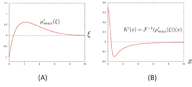
In (4.4), we use Bε(ξ):=eεξ2Bh(ξ)assignsubscriptsuperscript𝐵𝜀𝜉superscript𝑒𝜀superscript𝜉2subscript𝐵𝜉B^{\prime}_{\varepsilon}(\xi):=e^{-\varepsilon\xi^{2}}B_{h}(\xi) instead of Bε(ξ)subscript𝐵𝜀𝜉B_{\varepsilon}(\xi). Then all eigenvalues ζj(ξ)subscriptsuperscript𝜁𝑗𝜉\zeta^{\prime}_{j}(\xi) of Bε(ξ)subscriptsuperscript𝐵𝜀𝜉B^{\prime}_{\varepsilon}(\xi) satisfy ζj(ξ)0subscriptsuperscript𝜁𝑗𝜉0\zeta^{\prime}_{j}(\xi)\rightarrow 0 as |ξ|𝜉|\xi|\rightarrow\infty. Hence by adjusting ε𝜀\varepsilon and δ𝛿\delta appropriately such that Re(ζj(ξ))>1/δ𝑅𝑒subscriptsuperscript𝜁𝑗𝜉1𝛿Re(\zeta^{\prime}_{j}(\xi))>-1/\delta, we may take μ=ζj(ξ)𝜇subscriptsuperscript𝜁𝑗𝜉\mu=\zeta^{\prime}_{j}(\xi) as the solution of (4.7). Actually, Mmax(z)=zsubscript𝑀𝑚𝑎𝑥𝑧𝑧M_{max}(z)=z holds for z𝐂𝑧𝐂z\in{\bf C} with Re(z)>1/δ𝑅𝑒𝑧1𝛿Re(z)>-1/\delta and |Im(z)|C𝐼𝑚𝑧𝐶|Im(z)|\leq C for C>0𝐶0C>0 when 0<δ<<10𝛿much-less-than10<\delta<<1. Consequently, we can simply take μmax(ξ):=maxj{Re(ζj(ξ)}\mu^{\prime}_{max}(\xi):=\displaystyle\max_{j}\{Re(\zeta^{\prime}_{j}(\xi)\} instead of μmax(ξ)subscript𝜇𝑚𝑎𝑥𝜉\mu_{max}(\xi). In particular, μmax(ξ)=maxj{ζj(ξ)}subscriptsuperscript𝜇𝑚𝑎𝑥𝜉subscript𝑗subscriptsuperscript𝜁𝑗𝜉\mu^{\prime}_{max}(\xi)=\displaystyle\max_{j}\{\zeta^{\prime}_{j}(\xi)\} when ζj(ξ)𝐑subscriptsuperscript𝜁𝑗𝜉𝐑\zeta^{\prime}_{j}(\xi)\in{\bf R}. In Fig.10, the kernel K(x)=1(μmax(ξ))(x)superscript𝐾𝑥superscript1subscriptsuperscript𝜇𝑚𝑎𝑥𝜉𝑥K^{\prime}(x)={\cal F}^{-1}(\mu^{\prime}_{max}(\xi))(x) is drawn under the same parameters as Fig.8. It suggests that the essential structure of the original kernel K(x)𝐾𝑥K(x) is retained by this rough approximation.

Refer to caption
Figure 10: (A) Graph of μmax(ξ)=maxj{ζj(ξ)}subscriptsuperscript𝜇𝑚𝑎𝑥𝜉subscript𝑗subscriptsuperscript𝜁𝑗𝜉\mu^{\prime}_{max}(\xi)=\displaystyle\max_{j}\{\zeta^{\prime}_{j}(\xi)\} for the eigenvalues ζj(ξ)subscriptsuperscript𝜁𝑗𝜉\zeta^{\prime}_{j}(\xi) of Bε(ξ)subscriptsuperscript𝐵𝜀𝜉B^{\prime}_{\varepsilon}(\xi) . (B) The derived kernel K(x)=(1μmax)(x)superscript𝐾𝑥superscript1subscriptsuperscript𝜇𝑚𝑎𝑥𝑥K^{\prime}(x)=({\cal F}^{-1}\mu^{\prime}_{max})(x), which shows the Mexican hat profile. Parameters are same as those of Fig.6, Fig.8 and Fig.9: c1=c2=1subscript𝑐1subscript𝑐21c_{1}=c_{2}=1, c3=4subscript𝑐34c_{3}=4, c4=3subscript𝑐43c_{4}=3, d1=0.05subscript𝑑10.05d_{1}=0.05, d2=3subscript𝑑23d_{2}=3 and ε=0.05𝜀0.05\varepsilon=0.05. Only the right half pictures are drawn both in (A) and (B).

In the case of complex ζj(ξ)subscriptsuperscript𝜁𝑗𝜉\zeta^{\prime}_{j}(\xi) as in Section 4.2, we define b(ξ)superscript𝑏𝜉b^{\prime}(\xi), ωj(ξ)subscriptsuperscript𝜔𝑗𝜉\omega^{\prime}_{j}(\xi) and ω~j(ξ)subscriptsuperscript~𝜔𝑗𝜉\widetilde{\omega}^{\prime}_{j}(\xi) for ζj(ξ)subscriptsuperscript𝜁𝑗𝜉\zeta^{\prime}_{j}(\xi) in the same manners as b(ξ)𝑏𝜉b(\xi), ωj(ξ)subscript𝜔𝑗𝜉\omega_{j}(\xi) and ω~j(ξ)subscript~𝜔𝑗𝜉\widetilde{\omega}_{j}(\xi) for ζj(ξ)subscript𝜁𝑗𝜉\zeta_{j}(\xi). Then, we can take μ~j(ξ)=ω~j(ξ)subscriptsuperscript~𝜇𝑗𝜉subscriptsuperscript~𝜔𝑗𝜉\widetilde{\mu}^{\prime}_{j}(\xi)=\widetilde{\omega}^{\prime}_{j}(\xi) in (4.16), that is, μ~1(ξ)=ω1(ξ)+ib(ξ)subscriptsuperscript~𝜇1𝜉subscriptsuperscript𝜔1𝜉𝑖superscript𝑏𝜉\widetilde{\mu}^{\prime}_{1}(\xi)=\omega^{\prime}_{1}(\xi)+ib^{\prime}(\xi) and μ~2(ξ)=ω2(ξ)ib(ξ)subscriptsuperscript~𝜇2𝜉subscriptsuperscript𝜔2𝜉𝑖superscript𝑏𝜉\widetilde{\mu}^{\prime}_{2}(\xi)=\omega^{\prime}_{2}(\xi)-ib^{\prime}(\xi). Now we can calculate p~(ξ)superscript~𝑝𝜉\widetilde{p}^{\prime}(\xi), ν~j(ξ)subscriptsuperscript~𝜈𝑗𝜉\widetilde{\nu}^{\prime}_{j}(\xi) and q~(ξ)superscript~𝑞𝜉\widetilde{q}^{\prime}(\xi) corresponding to p~(ξ)~𝑝𝜉\widetilde{p}(\xi), ν~j(ξ)subscript~𝜈𝑗𝜉\widetilde{\nu}_{j}(\xi) and q~(ξ)~𝑞𝜉\widetilde{q}(\xi) respectively as follows:
Since μ~j(ξ)=ζj(ξ)subscriptsuperscript~𝜇𝑗𝜉subscriptsuperscript𝜁𝑗𝜉\widetilde{\mu}^{\prime}_{j}(\xi)=\zeta^{\prime}_{j}(\xi) for ξ<ξc𝜉subscript𝜉𝑐\xi<\xi_{c} and μ~1(ξ)=μ~2(ξ)¯=a(ξ)+ib(ξ)subscriptsuperscript~𝜇1𝜉¯subscriptsuperscript~𝜇2𝜉superscript𝑎𝜉𝑖superscript𝑏𝜉\widetilde{\mu}^{\prime}_{1}(\xi)=\overline{\widetilde{\mu}^{\prime}_{2}(\xi)}=a^{\prime}(\xi)+ib^{\prime}(\xi) for ξ>ξc𝜉subscript𝜉𝑐\xi>\xi_{c}, we see a~(ξ)=a(ξ)superscript~𝑎𝜉superscript𝑎𝜉\widetilde{a}^{\prime}(\xi)=a^{\prime}(\xi), b~(ξ)=b(ξ)superscript~𝑏𝜉superscript𝑏𝜉\widetilde{b}^{\prime}(\xi)=b^{\prime}(\xi) and therefore we get

p~(ξ):={μ~2(ξ)μ~1(ξ)ζ2(ξ)ζ1(ξ)=1(ξ<ξc),p~c:=1(ξ=ξc),b~(ξ)b(ξ)=1(ξ>ξc),assignsuperscript~𝑝𝜉casessubscriptsuperscript~𝜇2𝜉subscriptsuperscript~𝜇1𝜉subscriptsuperscript𝜁2𝜉subscriptsuperscript𝜁1𝜉absent1𝜉subscript𝜉𝑐subscriptsuperscript~𝑝𝑐assignabsent1𝜉subscript𝜉𝑐superscript~𝑏𝜉superscript𝑏𝜉absent1𝜉subscript𝜉𝑐\widetilde{p}^{\prime}(\xi):=\left\{\begin{array}[]{clc}\frac{\widetilde{\mu}^{\prime}_{2}(\xi)-\widetilde{\mu}^{\prime}_{1}(\xi)}{\zeta^{\prime}_{2}(\xi)-\zeta^{\prime}_{1}(\xi)}&=1&(\xi<\xi_{c}),\\ \widetilde{p}^{\prime}_{c}&:=1&(\xi=\xi_{c}),\\ \frac{\widetilde{b}^{\prime}(\xi)}{b^{\prime}(\xi)}&=1&(\xi>\xi_{c}),\end{array}\right. (4.39)
ν~j(ξ):={μ~j(ξ)=ζj(ξ)(ξξc),a~(ξ)=a(ξ)(ξ>ξc),assignsubscriptsuperscript~𝜈𝑗𝜉casessubscriptsuperscript~𝜇𝑗𝜉subscriptsuperscript𝜁𝑗𝜉𝜉subscript𝜉𝑐superscript~𝑎𝜉superscript𝑎𝜉𝜉subscript𝜉𝑐\widetilde{\nu}^{\prime}_{j}(\xi):=\left\{\begin{array}[]{ll}\widetilde{\mu}^{\prime}_{j}(\xi)=\zeta^{\prime}_{j}(\xi)&(\xi\leq\xi_{c}),\\ \widetilde{a}^{\prime}(\xi)=a^{\prime}(\xi)&(\xi>\xi_{c}),\end{array}\right. (4.40)

and

q~(ξ):={0(ξξc),b~(ξ)b(ξ)={b(ξ)}2(ξ>ξc).assignsuperscript~𝑞𝜉cases0𝜉subscript𝜉𝑐superscript~𝑏𝜉superscript𝑏𝜉superscriptsuperscript𝑏𝜉2𝜉subscript𝜉𝑐\widetilde{q}^{\prime}(\xi):=\left\{\begin{array}[]{ll}0&(\xi\leq\xi_{c}),\\ -\widetilde{b}^{\prime}(\xi)b^{\prime}(\xi)=-\{b^{\prime}(\xi)\}^{2}&(\xi>\xi_{c}).\end{array}\right. (4.41)

Thus, the effective equation is obtained as

{X˙=X+KX+Y,Y˙=Y+MX+NY,cases˙𝑋𝑋superscript𝐾𝑋𝑌˙𝑌𝑌superscript𝑀𝑋superscript𝑁𝑌\left\{\begin{array}[]{ccl}\dot{X}&=&{\cal L}X+K^{\prime}*X+Y,\\ \dot{Y}&=&{\cal L}Y+M^{\prime}*X+N^{\prime}*Y,\end{array}\right. (4.42)

where K(x):=1(ν~1(ξ))(x)assignsuperscript𝐾𝑥superscript1subscriptsuperscript~𝜈1𝜉𝑥K^{\prime}(x):={\cal F}^{-1}(\widetilde{\nu}^{\prime}_{1}(\xi))(x), M(x):=1(q~(ξ))(x)assignsuperscript𝑀𝑥superscript1superscript~𝑞𝜉𝑥M^{\prime}(x):={\cal F}^{-1}(\widetilde{q}^{\prime}(\xi))(x), N(x):=1(ν~2(ξ))(x)assignsuperscript𝑁𝑥superscript1subscriptsuperscript~𝜈2𝜉𝑥N^{\prime}(x):={\cal F}^{-1}(\widetilde{\nu}^{\prime}_{2}(\xi))(x) and the differential operator :=1(λh(ξ))assignsuperscript1subscript𝜆𝜉{\cal L}:={\cal F}^{-1}(\lambda_{h}(\xi)).

5 Applications

In previous sections, we only dealt with 1D problems just for simplicity while 2D problems should be considered as more realistic situations. Hence, some of the following applications, we consider 1D and 2D problems. In 2D case, x2superscriptsubscript𝑥2\partial_{x}^{2} is replaced with the Laplacian Δ=x2+y2Δsuperscriptsubscript𝑥2superscriptsubscript𝑦2\Delta=\partial_{x}^{2}+\partial_{y}^{2} and the Heat kernel Hε(x)subscript𝐻𝜀𝑥H_{\varepsilon}(x) on 1D is done with Hε(𝐱)=14πεer24εsubscript𝐻𝜀𝐱14𝜋𝜀superscript𝑒superscript𝑟24𝜀H_{\varepsilon}({\bf x})=\displaystyle\frac{1}{4\pi\varepsilon}e^{-\frac{r^{2}}{4\varepsilon}} for 𝐱=(x,y)𝐑2𝐱𝑥𝑦superscript𝐑2{\bf x}=(x,y)\in{\bf R}^{2}, r=x2+y2𝑟superscript𝑥2superscript𝑦2r=\sqrt{x^{2}+y^{2}} and so on.

The numerical simulations on spatial patterns are done by using the equation

ut=u+χ(u)(Kju),subscript𝑢𝑡𝑢𝜒𝑢subscript𝐾𝑗𝑢u_{t}={\cal L}u+\chi(u)\cdot(K_{j}*u), (5.1)

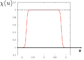
where Kj=K1(x)subscript𝐾𝑗subscript𝐾1𝑥K_{j}=K_{1}(x) (1D kernel ) or K2(x,y)subscript𝐾2𝑥𝑦K_{2}(x,y) (2D kernel) and {\cal L}, the derived kernels and differential operator in the manner of this paper, and χ(u)𝜒𝑢\chi(u) is a cut-off function satisfying 0χ(u)10𝜒𝑢10\leq\chi(u)\leq 1 and χ(u)=0𝜒𝑢0\chi(u)=0 for |u|u𝑢superscript𝑢|u|\geq u^{*} as in Figure 11.

Refer to caption
Figure 11: An example of the functional form of χ(u)𝜒𝑢\chi(u) in the case of u=1superscript𝑢1u^{*}=1.

5.1 Three node reaction-diffusion network

In this subsection, we consider the three node network as in Figure 12 dealt with in [14] as Type III network. The typical property of this example is that v𝑣v and w𝑤w diffuse with the same diffusion coefficients d>0𝑑0d>0 and u𝑢u does not move. In order to derive an effective kernel of this network, we use the notations in Section 2. Let U=(u,v,w)tU={{}^{t}}(u,v,w). In this network, the diffusion matrix D𝐷D is given by D=diag{0,d,d}𝐷𝑑𝑖𝑎𝑔0𝑑𝑑D=diag\{0,d,d\}. The matrix A𝐴A describing the network is A=(0k20k3k4k6k70k9)𝐴0subscript𝑘20subscript𝑘3subscript𝑘4subscript𝑘6subscript𝑘70subscript𝑘9A=\left(\begin{array}[]{ccc}0&k_{2}&0\\ k_{3}&-k_{4}&-k_{6}\\ k_{7}&0&-k_{9}\end{array}\right). Then the corresponding equation to (4.2) leads U^t=B(ξ2)U^subscript^𝑈𝑡𝐵superscript𝜉2^𝑈\widehat{U}_{t}=B(\xi^{2})\widehat{U} in 1D and U^t=B(R2)U^subscript^𝑈𝑡𝐵superscript𝑅2^𝑈\widehat{U}_{t}=B(R^{2})\widehat{U} in 2D with R=ξ2+η2𝑅superscript𝜉2superscript𝜂2R=\sqrt{\xi^{2}+\eta^{2}}, where

B(s)𝐵𝑠\displaystyle B(s) =\displaystyle= sD+A𝑠𝐷𝐴\displaystyle-sD+A
=\displaystyle= sdiag{0,d,d}+A𝑠𝑑𝑖𝑎𝑔0𝑑𝑑𝐴\displaystyle-sdiag\{0,d,d\}+A
=\displaystyle= (0k20k3dsk4k6k70dsk9)0subscript𝑘20subscript𝑘3𝑑𝑠subscript𝑘4subscript𝑘6subscript𝑘70𝑑𝑠subscript𝑘9\displaystyle\left(\begin{array}[]{ccc}0&k_{2}&0\\ k_{3}&-ds-k_{4}&-k_{6}\\ k_{7}&0&-ds-k_{9}\end{array}\right)

for s=ξ2𝑠superscript𝜉2s=\xi^{2} or s=R2𝑠superscript𝑅2s=R^{2} depending on the spatial dimension. Letting λj(s)subscript𝜆𝑗𝑠\lambda_{j}(s) (j=1,2,3𝑗123j=1,2,3) be eigenvalues of B(s)𝐵𝑠B(s), we see λmax(s):=maxj{λj(s)}cassignsubscript𝜆𝑚𝑎𝑥𝑠subscript𝑗subscript𝜆𝑗𝑠𝑐\lambda_{max}(s):=\displaystyle\max_{j}\{\lambda_{j}(s)\}\rightarrow c as s𝑠s\rightarrow\infty for c𝐑𝑐𝐑c\in{\bf R}. Hence by virtue of the way in Section 4.1, we take λh(s)=0subscript𝜆𝑠0\lambda_{h}(s)=0 and Bh(s)=B(s)subscript𝐵𝑠𝐵𝑠B_{h}(s)=B(s). Since Bh(s)=sD+Asubscript𝐵𝑠𝑠𝐷𝐴B_{h}(s)=-sD+A, we should deal with Bε(s)=sD+eεsAsubscript𝐵𝜀𝑠𝑠𝐷superscript𝑒𝜀𝑠𝐴B_{\varepsilon}(s)=-sD+e^{-\varepsilon s}A for 0<ε<<10𝜀much-less-than10<\varepsilon<<1 by the manner stated in Section 4.1. But here we use a simpler way stated in Practical way II) and put Bε(s)=eεsBh(s)subscriptsuperscript𝐵𝜀𝑠superscript𝑒𝜀𝑠subscript𝐵𝑠B^{\prime}_{\varepsilon}(s)=e^{-\varepsilon s}B_{h}(s). Then μmax(s)subscriptsuperscript𝜇𝑚𝑎𝑥𝑠\mu^{\prime}_{max}(s) is given by μmax(s)=maxj{ζj(s)σ(Bε(s))}subscriptsuperscript𝜇𝑚𝑎𝑥𝑠subscript𝑗subscriptsuperscript𝜁𝑗𝑠𝜎subscriptsuperscript𝐵𝜀𝑠\mu^{\prime}_{max}(s)=\displaystyle\max_{j}\{\zeta^{\prime}_{j}(s)\in\sigma(B^{\prime}_{\varepsilon}(s))\}.

In Fig.13, the first, second and third maximal eigenvalues of Bε(s)subscriptsuperscript𝐵𝜀𝑠B^{\prime}_{\varepsilon}(s) are drawn and also the 1D and 2D kernels K1(x)=1(μmax(ξ2))(x)subscriptsuperscript𝐾1𝑥superscript1subscriptsuperscript𝜇𝑚𝑎𝑥superscript𝜉2𝑥K^{\prime}_{1}(x)={\cal F}^{-1}(\mu^{\prime}_{max}(\xi^{2}))(x) and K2(r)=1(μmax(R2))(r)subscriptsuperscript𝐾2𝑟superscript1subscriptsuperscript𝜇𝑚𝑎𝑥superscript𝑅2𝑟K^{\prime}_{2}(r)={\cal F}^{-1}(\mu^{\prime}_{max}(R^{2}))(r), which shows that the effective kernel Kj(x)subscriptsuperscript𝐾𝑗𝑥K^{\prime}_{j}(x) has a Mexican hat profile and we can understand the LALI effect essentially occurs even if the diffusion constants are same.
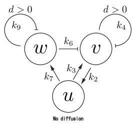
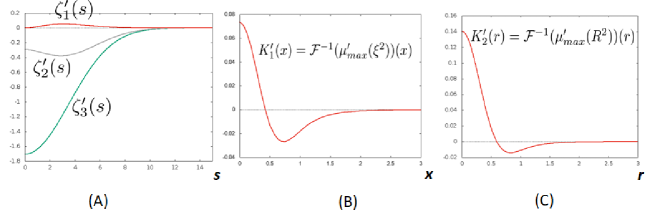
Refer to caption
Figure 12: Three node network. The picture is cited from [14] with the same notations as in Appendix 3-figure 4 in [14].
Refer to caption
Figure 13: (A) Eigenvalues of Bε(s)subscriptsuperscript𝐵𝜀𝑠B^{\prime}_{\varepsilon}(s), (B) The kernel K1(x)=1(μmax(ξ2))subscriptsuperscript𝐾1𝑥superscript1subscriptsuperscript𝜇𝑚𝑎𝑥superscript𝜉2K^{\prime}_{1}(x)={\cal F}^{-1}(\mu^{\prime}_{max}(\xi^{2})) on 1D, (C) The kernel K2(r)=1(μmax(R2))subscriptsuperscript𝐾2𝑟superscript1subscriptsuperscript𝜇𝑚𝑎𝑥superscript𝑅2K^{\prime}_{2}(r)={\cal F}^{-1}(\mu^{\prime}_{max}(R^{2})) on 2D. Parameter values are k2=0.5subscript𝑘20.5k_{2}=0.5, k3=k4=k6=k7=k9=1subscript𝑘3subscript𝑘4subscript𝑘6subscript𝑘7subscript𝑘91k_{3}=k_{4}=k_{6}=k_{7}=k_{9}=1, d=0.02𝑑0.02d=0.02 and ε=0.05𝜀0.05\varepsilon=0.05. All values except ε𝜀\varepsilon are same as in Appendix 3-figure 4 in [14].

5.2 Two node reaction-diffusion network with long range interaction

We apply the method to a problem including long range interaction in the network, which was stated in [15], [22] for interactions between zebra-fish pigment cells. The schematic picture of the network is like Fig.14. The long range interaction means a cell interact directly to cells at a constant distant location by e.g. projections as in Figure 4 and we may represent the effect by the kernel Ll(x):=12{δ(x+l)+δ(xl)}assignsubscript𝐿𝑙𝑥12𝛿𝑥𝑙𝛿𝑥𝑙L_{l}(x):=\frac{1}{2}\{\delta(x+l)+\delta(x-l)\} for x𝐑𝑥𝐑x\in{\bf R} and Ll(x,y):=12πlδ(|𝐱|l)assignsubscript𝐿𝑙𝑥𝑦12𝜋𝑙𝛿𝐱𝑙L_{l}(x,y):=\frac{1}{2\pi l}\delta(|{\bf x}|-l) for 𝐱=(x,y)𝐑2𝐱𝑥𝑦superscript𝐑2{\bf x}=(x,y)\in{\bf R}^{2}, where l𝑙l is a positive constant. Let u𝑢u and v𝑣v be the differences from some rest states of densities of the two types of pigment cells, melanophores and xanthophores, respectively ([15]). Then the matrix A𝐴A describing the network according to Fig.14 is

AU=(k1Llk5k3+k4Llk2k6)U=(k1Lluk5uk3v+k4Llvk2uk6v)AU=\left(\begin{array}[]{cc}-k_{1}L_{l}*-k_{5}&-k_{3}+k_{4}L_{l}*\\ -k_{2}&-k_{6}\end{array}\right)U=\left(\begin{array}[]{c}-k_{1}L_{l}*u-k_{5}u-k_{3}v+k_{4}L_{l}*v\\ -k_{2}u-k_{6}v\end{array}\right)

for U=(u,v)tU={{}^{t}}(u,v). In [15], it was simulated with the same small diffusion constants of u𝑢u and v𝑣v. Hence we also assume u𝑢u and v𝑣v spatially diffuse with the same diffusion constant d𝑑d. Then the corresponding equation to (4.1) is

Ut=DΔU+AU,subscript𝑈𝑡𝐷Δ𝑈𝐴𝑈U_{t}=D\Delta U+AU,

where D=diag{d,d}𝐷𝑑𝑖𝑎𝑔𝑑𝑑D=diag\{d,d\}. Taking the Fourier transformation of the above equation, we have

U^t=B1(ξ)U^(1Dcase),U^t=B2(R)U^(2Dcase),formulae-sequencesubscript^𝑈𝑡subscript𝐵1𝜉^𝑈1𝐷𝑐𝑎𝑠𝑒subscript^𝑈𝑡subscript𝐵2𝑅^𝑈2𝐷𝑐𝑎𝑠𝑒\hat{U}_{t}=B_{1}(\xi)\hat{U}\;\;(1D\;case),\;\hat{U}_{t}=B_{2}(R)\hat{U}\;\;(2D\;case),

where R=ξ2+η2𝑅superscript𝜉2superscript𝜂2R=\sqrt{\xi^{2}+\eta^{2}} and

Bj(s)=(ds2k1Ll^(s)k5k3+k4Ll^(s)k2ds2k6)subscript𝐵𝑗𝑠𝑑superscript𝑠2subscript𝑘1^subscript𝐿𝑙𝑠subscript𝑘5subscript𝑘3subscript𝑘4^subscript𝐿𝑙𝑠subscript𝑘2𝑑superscript𝑠2subscript𝑘6B_{j}(s)=\left(\begin{array}[]{cc}-ds^{2}-k_{1}\widehat{L_{l}}(s)-k_{5}&-k_{3}+k_{4}\widehat{L_{l}}(s)\\ -k_{2}&-ds^{2}-k_{6}\end{array}\right)

for s=ξ𝑠𝜉s=\xi in 1D or s=R𝑠𝑅s=R in 2D. Here, Ll^^subscript𝐿𝑙\widehat{L_{l}} is computed for 1D,

Ll^(ξ)=12(eiξl+eiξl)δ^(ξ)=cosξl=:P1(ξ)\widehat{L_{l}}(\xi)=\frac{1}{2}(e^{i\xi l}+e^{-i\xi l})\widehat{\delta}(\xi)=\cos\xi l=:P_{1}(\xi)

and for 2D,

12πlLl^(R)12𝜋𝑙^subscript𝐿𝑙𝑅\displaystyle\displaystyle\frac{1}{2\pi l}\widehat{L_{l}}(R) =\displaystyle= 00π/2rδ(rl)cos(rRsinθ)dθdr=12π0π/2cos(lRsinθ)dθdr=:P2(R)\displaystyle\!\displaystyle\int_{0}^{\infty}\!\!\!\!\displaystyle\int_{0}^{\pi/2}\!\!\!\!\!\!r\delta(r-l)\cos(rR\sin\theta)d\theta dr=\displaystyle\frac{1}{2\pi}\displaystyle\int_{0}^{\pi/2}\!\!\!\!\!\!\cos(lR\sin\theta)d\theta dr=:P_{2}(R)

by using (5.1). Thus we find

Bj(s)=(ds2k1Pj(s)k5k3+k4Pj(s)k2ds2k6)subscript𝐵𝑗𝑠𝑑superscript𝑠2subscript𝑘1subscript𝑃𝑗𝑠subscript𝑘5subscript𝑘3subscript𝑘4subscript𝑃𝑗𝑠subscript𝑘2𝑑superscript𝑠2subscript𝑘6B_{j}(s)=\left(\begin{array}[]{cc}-ds^{2}-k_{1}P_{j}(s)-k_{5}&\;-k_{3}+k_{4}P_{j}(s)\\ -k_{2}&-ds^{2}-k_{6}\end{array}\right)

satisfying Bj(s)=Bj(s)subscript𝐵𝑗𝑠subscript𝐵𝑗𝑠B_{j}(-s)=B_{j}(s).

Let λ1,j(s)subscript𝜆1𝑗𝑠\lambda_{1,j}(s) and λ2,j(s)subscript𝜆2𝑗𝑠\lambda_{2,j}(s) be eigenvalues of Bj(s)subscript𝐵𝑗𝑠B_{j}(s). Since eigenvalues have the asymptotic profile in the highest order of s𝑠s as λi,j(s)ds2+O(1)subscript𝜆𝑖𝑗𝑠𝑑superscript𝑠2𝑂1\lambda_{i,j}(s)\rightarrow-ds^{2}+O(1) as s𝑠s\rightarrow\infty, we take λh(s)=ds2subscript𝜆𝑠𝑑superscript𝑠2\lambda_{h}(s)=-ds^{2} and Bj,h(s)={Bj(s)+ds2I}subscript𝐵𝑗𝑠subscript𝐵𝑗𝑠𝑑superscript𝑠2𝐼B_{j,h}(s)=\{B_{j}(s)+ds^{2}I\} according to Section 4.1. Since Bj,h(s)=O(1)subscript𝐵𝑗𝑠𝑂1B_{j,h}(s)=O(1), we put Bj,ε(s)=eεs2Bj,h(s)subscript𝐵𝑗𝜀𝑠superscript𝑒𝜀superscript𝑠2subscript𝐵𝑗𝑠B_{j,\varepsilon}(s)=e^{-\varepsilon s^{2}}B_{j,h}(s). Then μmax(s)subscript𝜇𝑚𝑎𝑥𝑠\mu_{max}(s) may be calculated by using the approximation stated in Practical way II) as μmax(s)=maxj{ζi,j(s)σ(Bi,ε(s)}\mu_{max}(s)=\displaystyle\max_{j}\{\zeta_{i,j}(s)\in\sigma(B_{i,\varepsilon}(s)\} and we get the effective equation by

(1D):wt=dwxx+K1w,(2D):wt=dΔw+K2w.:1𝐷subscript𝑤𝑡𝑑subscript𝑤𝑥𝑥subscript𝐾1𝑤2𝐷:subscript𝑤𝑡𝑑Δ𝑤subscript𝐾2𝑤(1D):w_{t}=dw_{xx}+K_{1}*w,\;\;(2D):w_{t}=d\Delta w+K_{2}*w.

In Fig.15, μmax(s)subscript𝜇𝑚𝑎𝑥𝑠\mu_{max}(s) of B1(s)subscript𝐵1𝑠B_{1}(s) and B2(s)subscript𝐵2𝑠B_{2}(s) are respectively drawn together with the reduced kernels in 1D and 2D for the case corresponding to the simulation in [15]. Fig.16 and Fig.17 are numerical simulations for 2D patterns by using the reduced equation wt=dΔw+χ(w)(K2w)subscript𝑤𝑡𝑑Δ𝑤𝜒𝑤subscript𝐾2𝑤w_{t}=d\Delta w+\chi(w)\cdot(K_{2}*w) with the kernel K2(r)subscript𝐾2𝑟K_{2}(r) in Fig.15, which shows that the similar patterns to [15] appear. Here, we should note that the system of u𝑢u and v𝑣v without long range interactions (corresponding to the case of k1=k4=0subscript𝑘1subscript𝑘40k_{1}=k_{4}=0 in Figure 14) is unstable in the kinetics, that is, the matrix (k5k3k2k6)subscript𝑘5subscript𝑘3subscript𝑘2subscript𝑘6\left(\begin{array}[]{cc}-k_{5}&-k_{3}\\ -k_{2}&-k_{6}\end{array}\right) has eigenvalues with positive real parts under the parameter values in Figure 15. In [15], it was demonstrated that the Turing pattern appears by introducing the third component w𝑤w, which plays the role of long range interactions. In this subsection, the long range interactions are directly introduced by Llsubscript𝐿𝑙L_{l} and the Turing pattern is naturally observed in 2D as in (C) of Figure 15, that is, λ1(0)<0subscript𝜆100\lambda_{1}(0)<0 in (C). Thus, the method in this paper does not require any artificial treatment and make the direct understanding of the mechanism possible through the reduced kernels.

Remark 5.1.

In Fig.15 (A), we observe λ1(0)>0subscript𝜆100\lambda_{1}(0)>0, which means that the Turing pattern does not appear in 1D case for any l>0𝑙0l>0. Actually, the functional form of P1(ξ)2cosξlsimilar-tosubscript𝑃1𝜉2𝜉𝑙P_{1}(\xi)\sim 2\cos\xi l leads P1(0)=2subscript𝑃102P_{1}(0)=2 independent of l𝑙l and the matrix B1(0)subscript𝐵10B_{1}(0) has an positive eigenvalue under the parameter values in Fig.15 while in 2D, P2(0)=2πlsubscript𝑃202𝜋𝑙P_{2}(0)=2\pi l holds and the maximal eigenvalue λ1(0)subscript𝜆10\lambda_{1}(0) of B2(0)subscript𝐵20B_{2}(0) can be negative depending on l𝑙l.

Refer to caption
Figure 14: Deduced interaction network between pigment cells of Zebra-fish, which is referred from [15, 22]. The coefficient k1subscript𝑘1k_{1} is possibly equal to zero ([22]).
Refer to caption
Figure 15: (A) μmax(s)subscript𝜇𝑚𝑎𝑥𝑠\mu_{max}(s) of B1(s)subscript𝐵1𝑠B_{1}(s), (B) The kernel K1(x)=1(μmax(ξ))(x)subscript𝐾1𝑥superscript1subscript𝜇𝑚𝑎𝑥𝜉𝑥K_{1}(x)={\cal F}^{-1}(\mu_{max}(\xi))(x) by B1(s)subscript𝐵1𝑠B_{1}(s), (C) μmax(s)subscript𝜇𝑚𝑎𝑥𝑠\mu_{max}(s) of B2(s)subscript𝐵2𝑠B_{2}(s), (D) The kernel K2(r)=1(μmax(R))(x)subscript𝐾2𝑟superscript1subscript𝜇𝑚𝑎𝑥𝑅𝑥K_{2}(r)={\cal F}^{-1}(\mu_{max}(R))(x) by B2(s)subscript𝐵2𝑠B_{2}(s). Parameters are d=0.02𝑑0.02d=0.02, k1=0.0550.016subscript𝑘10.0550.016k_{1}=0.055*0.016, k2=0.05subscript𝑘20.05k_{2}=0.05, k3=0.04subscript𝑘30.04k_{3}=0.04, k4=0.0550.03subscript𝑘40.0550.03k_{4}=0.055*0.03, k5=0.02subscript𝑘50.02k_{5}=0.02, k6=0.025subscript𝑘60.025k_{6}=0.025. which are adjusted to parameter values for a wild type of Fig 4 in [15]. l𝑙l and ε𝜀\varepsilon are given by l=3𝑙3l=3 and ε=0.05𝜀0.05\varepsilon=0.05.
Refer to caption
Figure 16: Time evolution of spatial patterns in 2D by the kernel K2(r)subscript𝐾2𝑟K_{2}(r) in Fig.15 (D) using (5.1) with u=1superscript𝑢1u^{*}=1. The initial condition is set similarly to that of the numerical simulations reported in [15].
Refer to caption
Figure 17: Time evolution of spatial patterns in 2D with initial data added a random ablated region by the kernel K2(r)subscript𝐾2𝑟K_{2}(r) in Fig.15 (D) using (5.1) with u=1superscript𝑢1u^{*}=1.

In the last of this subsection, we show numerical simulations comparing two cases of k10subscript𝑘10k_{1}\neq 0 and k1=0subscript𝑘10k_{1}=0 because the self-inhibition of u𝑢u component is not assumed in [22]. Fig.18 shows the comparison of eigenvalues and the reduced kernels between the cases k10subscript𝑘10k_{1}\neq 0 and k1=0subscript𝑘10k_{1}=0. Fig.19 and Fig.20 show the numerical simulations in 2D patterns under the parameters of Fig.18. They strongly suggest that two situations with nonzero and zero k1subscript𝑘1k_{1} values exhibit almost same properties with respect to reduced kernels and 2D patterns.
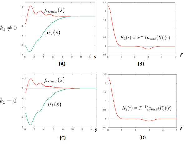
Refer to caption
Figure 18: Comparison between the cases of k1=5.50.0160subscript𝑘15.50.0160k_{1}=5.5*0.016\neq 0 and k1=0subscript𝑘10k_{1}=0. Other parameters are fixed by l=3.0𝑙3.0l=3.0, d=0.2𝑑0.2d=0.2, k2=5.0subscript𝑘25.0k_{2}=5.0, k3=4.0subscript𝑘34.0k_{3}=4.0, k4=5.50.03subscript𝑘45.50.03k_{4}=5.5*0.03, k5=3.0subscript𝑘53.0k_{5}=3.0, k6=3.0subscript𝑘63.0k_{6}=3.0. For k1=5.50.05subscript𝑘15.50.05k_{1}=5.5*0.05, (A) eigenvalues of B2(s)subscript𝐵2𝑠B_{2}(s), (B) the kernel K2(r)=1(μmax(R))(r)subscript𝐾2𝑟superscript1subscript𝜇𝑚𝑎𝑥𝑅𝑟K_{2}(r)={\cal F}^{-1}(\mu_{max}(R))(r). For k1=0subscript𝑘10k_{1}=0, (C) eigenvalues of B2(s)subscript𝐵2𝑠B_{2}(s), (D) the kernel K2(r)=1(μmax(R))(r)subscript𝐾2𝑟superscript1subscript𝜇𝑚𝑎𝑥𝑅𝑟K_{2}(r)={\cal F}^{-1}(\mu_{max}(R))(r).
Refer to caption
Figure 19: Comparison between the cases of k1=5.50.0160subscript𝑘15.50.0160k_{1}=5.5*0.016\neq 0 and k1=0subscript𝑘10k_{1}=0. Other parameters are fixed under the parameters of Fig.18. The upper picture is a time evolutional 2D pattern with the kernel K2(r)subscript𝐾2𝑟K_{2}(r) of Fig.18 (B) and the lower picture is the one with the kernel K2(r)subscript𝐾2𝑟K_{2}(r) of Fig.18 (D). The initial data is the same one as Fig.16.
Refer to caption
Figure 20: Comparison between the cases of k1=5.50.0160subscript𝑘15.50.0160k_{1}=5.5*0.016\neq 0 and k1=0subscript𝑘10k_{1}=0. Other parameters are fixed under the parameters of Fig.18. The upper picture is a time evolutional 2D pattern with the kernel K2(r)subscript𝐾2𝑟K_{2}(r) of Fig.18 (B) and the lower picture is the one with the kernel K2(r)subscript𝐾2𝑟K_{2}(r) of Fig.18 (D). The initial data is the same one as Fig.17 added a random ablated region.

5.3 Network for Proneural waves

Refer to caption
Figure 21: The proneural wave progresses unidirectionally during optic lobe development in Drosophila. (A) A schematic of the progression of the proneural wave. The proneural wave sweeps from medial to lateral. L’sc is transiently expressed in the differentiating neuroepithelial cells (NEs) and defines the timing of the differentiation of the NE to the neuroblast (NB). EGF positively regulates the progression of the wave, while Notch negatively regulates wave progression through increasing the expression of Notch target genes. (B) Schema showing the gene regulatory network including AS-C, EGF, Notch and Delta. (C) Lateral inhibition mechanism of Delta/Notch signaling.

It was reported in [20] that regulated waves of differentiation called the “proneural wave” is observed in visual systems on the surface of the brain of the fruit fly. The phenomena was modeled in a mathematical PDE model as the Delta-Notch system including variables E𝐸E, N𝑁N, D𝐷D and Assubscript𝐴𝑠A_{s} corresponding to the EGF ligand concentration and EGF signaling (E𝐸E), Notch signal activity (N𝑁N), Delta expression (D𝐷D) and the level of the differentiation of AS-C in cells (Assubscript𝐴𝑠A_{s}), respectively. The network of the molecular interactions is as in Fig.21 (B). The typical properties of the network is that E𝐸E diffuses and other materials do not and that D𝐷D inhibits N𝑁N in the same cell while it activates N𝑁N in contiguous cells (Fig.21 (C)). Then by denoting the distance between a cell and the contiguous cells by l>0𝑙0l>0, the matrix A𝐴A describing the network drawn in Fig.21 is given by

AU=(ke00ae0kndtLldc000kdadeaea00)U=(keE+aeAsknN+dtLlDdcDkdD+adAsea(EN))AU=\left(\begin{array}[]{cccc}-k_{e}&0&0&a_{e}\\ 0&-k_{n}&d_{t}L_{l}*-d_{c}&0\\ 0&0&-k_{d}&a_{d}\\ e_{a}&-e_{a}&0&0\end{array}\right)U=\left(\begin{array}[]{c}-k_{e}E+a_{e}A_{s}\\ -k_{n}N+d_{t}L_{l}*D-d_{c}D\\ -k_{d}D+a_{d}A_{s}\\ e_{a}(E-N)\end{array}\right)

for U=(E,N,D,As)tU={{}^{t}}(E,N,D,A_{s}). Here we used the same functions and notations as those in the previous subsections such as Pj(s)subscript𝑃𝑗𝑠P_{j}(s). The equation is

Ut=DΔU+AU,subscript𝑈𝑡𝐷Δ𝑈𝐴𝑈U_{t}=D\Delta U+AU,

where D=diag{de,0,0,0}𝐷𝑑𝑖𝑎𝑔subscript𝑑𝑒000D=diag\{d_{e},0,0,0\}. The Fourier transformation leads U^t=B1(ξ)U^subscript^𝑈𝑡subscript𝐵1𝜉^𝑈\widehat{U}_{t}=B_{1}(\xi)\widehat{U} (1D case) and U^t=B2(R)U^subscript^𝑈𝑡subscript𝐵2𝑅^𝑈\widehat{U}_{t}=B_{2}(R)\widehat{U} (2D case), where R=ξ2+η2𝑅superscript𝜉2superscript𝜂2R=\sqrt{\xi^{2}+\eta^{2}}, Bj(s)=s2D+A^j(s)subscript𝐵𝑗𝑠superscript𝑠2𝐷subscript^𝐴𝑗𝑠B_{j}(s)=-s^{2}D+\widehat{A}_{j}(s) and

A^j(s)=(ke00ae0kndtPj(s)dc000kdadeaea00).subscript^𝐴𝑗𝑠subscript𝑘𝑒00subscript𝑎𝑒0subscript𝑘𝑛subscript𝑑𝑡subscript𝑃𝑗𝑠subscript𝑑𝑐000subscript𝑘𝑑subscript𝑎𝑑subscript𝑒𝑎subscript𝑒𝑎00\widehat{A}_{j}(s)=\left(\begin{array}[]{cccc}-k_{e}&0&0&a_{e}\\ 0&-k_{n}&d_{t}P_{j}(s)-d_{c}&0\\ 0&0&-k_{d}&a_{d}\\ e_{a}&-e_{a}&0&0\end{array}\right).

Since the maximal eigenvalue of Bj(s)subscript𝐵𝑗𝑠B_{j}(s) is O(1)𝑂1O(1), we take λh(s)=0subscript𝜆𝑠0\lambda_{h}(s)=0, Bj,h(s)=Bj(s)=s2D+A^j(s)subscript𝐵𝑗𝑠subscript𝐵𝑗𝑠superscript𝑠2𝐷subscript^𝐴𝑗𝑠B_{j,h}(s)=B_{j}(s)=-s^{2}D+\widehat{A}_{j}(s) with A^j(s)=O(1)subscript^𝐴𝑗𝑠𝑂1\widehat{A}_{j}(s)=O(1) and therefore we should put Bj,ε(s)=s2D+eεs2A^j(s)subscript𝐵𝑗𝜀𝑠superscript𝑠2𝐷superscript𝑒𝜀superscript𝑠2subscript^𝐴𝑗𝑠B_{j,\varepsilon}(s)=-s^{2}D+e^{-\varepsilon s^{2}}\widehat{A}_{j}(s) according to the manner in Section 4. But, here we use the simplest case of Bj,ε(s)=eεs2Bj,h(s)subscriptsuperscript𝐵𝑗𝜀𝑠superscript𝑒𝜀superscript𝑠2subscript𝐵𝑗𝑠B^{\prime}_{j,\varepsilon}(s)=e^{-\varepsilon s^{2}}B_{j,h}(s) according to Practical way II) and only consider 2 dimensional problems (the case of s=R=ξ2+η2𝑠𝑅superscript𝜉2superscript𝜂2s=R=\sqrt{\xi^{2}+\eta^{2}}). The effective equations are as follows:

When all eigenvalues ζj(R)subscriptsuperscript𝜁𝑗𝑅\zeta^{\prime}_{j}(R) of Bj,ε(R)subscriptsuperscript𝐵𝑗𝜀𝑅B^{\prime}_{j,\varepsilon}(R) are real, the effective equation is wt=K2wsubscript𝑤𝑡subscriptsuperscript𝐾2𝑤w_{t}=K^{\prime}_{2}*w, where K2(r)=1(μmax(R))(r)subscriptsuperscript𝐾2𝑟superscript1subscriptsuperscript𝜇𝑚𝑎𝑥𝑅𝑟K^{\prime}_{2}(r)={\cal F}^{-1}(\mu^{\prime}_{max}(R))(r) and μmax(R)=maxj{ζj(R)}subscriptsuperscript𝜇𝑚𝑎𝑥𝑅subscript𝑗subscriptsuperscript𝜁𝑗𝑅\mu^{\prime}_{max}(R)=\displaystyle\max_{j}\{\zeta^{\prime}_{j}(R)\} for r=x2+y2𝑟superscript𝑥2superscript𝑦2r=\sqrt{x^{2}+y^{2}}. In numerical simulations, the equation

wt=χ(w)max{(K2w),0}w_{t}=\chi(w)\max\{\cdot(K^{\prime}_{2}*w),0\} (5.3)

is treated because of the irreversibility of the differentiation of cells, which will require the monotonicity in time and the modification in (5.3) seems natural. In Fig.22, μmax(R)subscriptsuperscript𝜇𝑚𝑎𝑥𝑅\mu^{\prime}_{max}(R) and the reduced kernel are drawn in the case that eigenvalues of Bj,ε(s)subscriptsuperscript𝐵𝑗𝜀𝑠B^{\prime}_{j,\varepsilon}(s) are all real. Fig.23 draws the numerical simulation of (5.3) by using the kernel K2(r)subscriptsuperscript𝐾2𝑟K^{\prime}_{2}(r) in Fig.22. It shows a stable traveling planar pattern appears corresponding to the proneural wave.
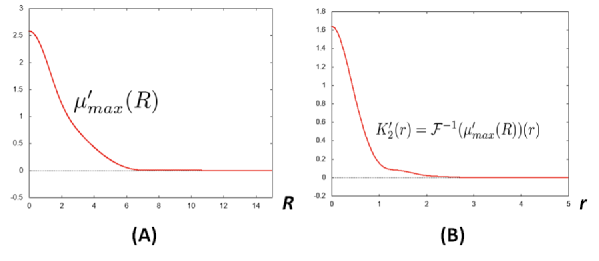
Refer to caption
Figure 22: (A)  μmax(R)subscriptsuperscript𝜇𝑚𝑎𝑥𝑅\mu^{\prime}_{max}(R) obtained from B2,ε(s)subscriptsuperscript𝐵2𝜀𝑠B^{\prime}_{2,\varepsilon}(s). (B)  The reduced kernel from μmax(R)subscriptsuperscript𝜇𝑚𝑎𝑥𝑅\mu^{\prime}_{max}(R). The parameter values are de=1.0subscript𝑑𝑒1.0d_{e}=1.0, ke=1.0subscript𝑘𝑒1.0k_{e}=1.0, ae=1.0subscript𝑎𝑒1.0a_{e}=1.0, kn=2.0subscript𝑘𝑛2.0k_{n}=2.0, dt=0.5/(2πl)subscript𝑑𝑡0.52𝜋𝑙d_{t}=0.5/(2\pi l), dc=0.1subscript𝑑𝑐0.1d_{c}=0.1, kd=1.5subscript𝑘𝑑1.5k_{d}=1.5, ad=1.0subscript𝑎𝑑1.0a_{d}=1.0 and ea=10.0subscript𝑒𝑎10.0e_{a}=10.0. We also take l=1𝑙1l=1 and ϵ=0.05italic-ϵ0.05\epsilon=0.05.
Refer to caption
Figure 23: Time evolution of spatial pattern in 2D simulated by (5.3) with the kernel K2(r)subscriptsuperscript𝐾2𝑟K^{\prime}_{2}(r) of Fig.22, which shows a regulated propagation of proneural wave. Red color means the higher value of w𝑤w. Parameter values are same as those in Fig.22.

When the eigenvalue with maximal real part can be complex, we get (4.42) with =1(λh(R))=0superscript1subscript𝜆𝑅0{\cal L}={\cal F}^{-1}(\lambda_{h}(R))=0. that is

{X˙=K2X+Y,Y˙=M2X+N2Y,cases˙𝑋subscriptsuperscript𝐾2𝑋𝑌˙𝑌subscriptsuperscript𝑀2𝑋subscriptsuperscript𝑁2𝑌\left\{\begin{array}[]{ccl}\dot{X}&=&K^{\prime}_{2}*X+Y,\\ \dot{Y}&=&M^{\prime}_{2}*X+N^{\prime}_{2}*Y,\end{array}\right.

where K2(r)=1(ν~1(R))(r)subscriptsuperscript𝐾2𝑟superscript1subscriptsuperscript~𝜈1𝑅𝑟K^{\prime}_{2}(r)={\cal F}^{-1}(\widetilde{\nu}^{\prime}_{1}(R))(r), M2(r)=1(q~(R))(r)subscriptsuperscript𝑀2𝑟superscript1superscript~𝑞𝑅𝑟M^{\prime}_{2}(r)={\cal F}^{-1}(\widetilde{q}^{\prime}(R))(r) and N2(r)=1(ν~2(R))(r)subscriptsuperscript𝑁2𝑟superscript1subscriptsuperscript~𝜈2𝑅𝑟N^{\prime}_{2}(r)={\cal F}^{-1}(\widetilde{\nu}^{\prime}_{2}(R))(r). Numerical simulations are done by the following equation:

{X˙=χ(X)max{(K2X+Y),0},Y˙=χ(Y)(M2X+N2Y)cases˙𝑋𝜒𝑋subscriptsuperscript𝐾2𝑋𝑌0˙𝑌𝜒𝑌subscriptsuperscript𝑀2𝑋subscriptsuperscript𝑁2𝑌\left\{\begin{array}[]{ccl}\dot{X}&=&\chi(X)\max\{(K^{\prime}_{2}*X+Y),0\},\\ \dot{Y}&=&\chi(Y)(M^{\prime}_{2}*X+N^{\prime}_{2}*Y)\end{array}\right. (5.4)

because of the irreversibility of the differentiation of cells as stated for (5.3). In Fig.24, the reduced kernels K2(r)subscriptsuperscript𝐾2𝑟K^{\prime}_{2}(r), M2(r)subscriptsuperscript𝑀2𝑟M^{\prime}_{2}(r) and N2(r)subscriptsuperscript𝑁2𝑟N^{\prime}_{2}(r) are shown in the case when B2ε(R)subscriptsuperscript𝐵2𝜀𝑅B^{\prime}_{2\varepsilon}(R) can have complex eigenvalues. The parameter values are same as those of Fig.22 except the coefficient aesubscript𝑎𝑒a_{e}. In practice, ae=1subscript𝑎𝑒1a_{e}=1 in Fig.22 and ae=0.1subscript𝑎𝑒0.1a_{e}=0.1 in Fig.24. As in Fig.21 and also in the matrix A𝐴A, aesubscript𝑎𝑒a_{e} denotes the activation rate of Assubscript𝐴𝑠A_{s} (AS-C) for E𝐸E (EGF). Lower aesubscript𝑎𝑒a_{e} is expected to enhance the lateral inhibition by Delta/Notch signaling shown in Fig.21 (C) and as the consequence, pepper and salt patterns are caused as indicated in [20]. Fig.25 demonstrates the occurrence of salt and pepper patterns.
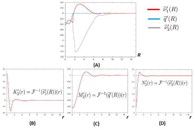
Refer to caption
Figure 24: (A)  ν~1(R)subscriptsuperscript~𝜈1𝑅\widetilde{\nu}^{\prime}_{1}(R), ν~2(R)subscriptsuperscript~𝜈2𝑅\widetilde{\nu}^{\prime}_{2}(R) and q~(R)superscript~𝑞𝑅\widetilde{q}^{\prime}(R) obtained from B2,ε(R)subscriptsuperscript𝐵2𝜀𝑅B^{\prime}_{2,\varepsilon}(R). (B), (C), (D) are the kernels obtained from them. The parameter values are de=1.0subscript𝑑𝑒1.0d_{e}=1.0, ke=1.0subscript𝑘𝑒1.0k_{e}=1.0, ae=0.1subscript𝑎𝑒0.1a_{e}=0.1, kn=2.0subscript𝑘𝑛2.0k_{n}=2.0, dt=0.5/(2πl)subscript𝑑𝑡0.52𝜋𝑙d_{t}=0.5/(2\pi l), dc=0.1subscript𝑑𝑐0.1d_{c}=0.1, kd=1.5subscript𝑘𝑑1.5k_{d}=1.5, ad=1.0subscript𝑎𝑑1.0a_{d}=1.0 and ea=10.0subscript𝑒𝑎10.0e_{a}=10.0. We also take l=1.0𝑙1.0l=1.0 and ϵ=0.05italic-ϵ0.05\epsilon=0.05. Only aesubscript𝑎𝑒a_{e} is changed smaller than the one in Fig.22 and Fig.23.
Refer to caption
Figure 25: Time evolution of spatial pattern in 2D simulated by (5.4) with kernels K2subscriptsuperscript𝐾2K^{\prime}_{2}, M2subscriptsuperscript𝑀2M^{\prime}_{2} and N2subscriptsuperscript𝑁2N^{\prime}_{2} computed in (B), (C) and (D) of Fig.24, which shows salt and pepper patterns. Only X𝑋X component is drawn. Parameter values are same as those of Fig.24.
Remark 5.2.

In this section, we adopted the heat kernel Hε(x)subscript𝐻𝜀𝑥H_{\varepsilon}(x) as the approximation of the Dirac δ𝛿\delta-function. If zero state is unstable as the grand state in a system, the approximation by the heat kernel may cause some trouble because the heat kernel Hϵsubscript𝐻italic-ϵH_{\epsilon} activates the instability everywhere by the property that (Hϵu)(x)>0subscript𝐻italic-ϵ𝑢𝑥0(H_{\epsilon}*u)(x)>0 everywhere for a function u(x)0𝑢𝑥0u(x)\geq 0. In that case, the approximation by the mollifier Jϵsubscript𝐽italic-ϵJ_{\epsilon} stated in Proposition 2.1 seems better because the mollifier can approximate supports, i.e., the support of Jϵusubscript𝐽italic-ϵ𝑢J_{\epsilon}*u is close to the support of u𝑢u. Then, we can replace Bj,ε(s)subscript𝐵𝑗𝜀𝑠B_{j,\varepsilon}(s) either by Bj,ε(s)=s2D+Jε^(s)A^j(s)subscriptsuperscript𝐵𝑗𝜀𝑠superscript𝑠2𝐷^subscript𝐽𝜀𝑠subscript^𝐴𝑗𝑠B^{*}_{j,\varepsilon}(s)=-s^{2}D+\widehat{J_{\varepsilon}}(s)\cdot\widehat{A}_{j}(s) or roughly Bj,ε(s)=Jε^(s)Bj(s)=Jε^(s){s2D+A^j(s)}subscriptsuperscript𝐵𝑗𝜀𝑠^subscript𝐽𝜀𝑠subscript𝐵𝑗𝑠^subscript𝐽𝜀𝑠superscript𝑠2𝐷subscript^𝐴𝑗𝑠B^{\prime}_{j,\varepsilon}(s)=\widehat{J_{\varepsilon}}(s)\cdot B_{j}(s)=\widehat{J_{\varepsilon}}(s)\cdot\{-s^{2}D+\widehat{A}_{j}(s)\}.

6 Discussion

The efficiency of KT models for the investigation of spatial patterns in biology was clearly mentioned in [8]. In this paper, we proposed a method to get the effective kernels from given network systems. Patterns generated from network systems are directly determined by the reduced kernels. It means even when given two network systems seem quite different each other, the two different network systems can be identified from the view point of patterns through the reduced effective kernels. The application stated in 5.1 is a typical example of that point. In practice, the effective kernel of the network of Fig.12 has a Mexican hat profile as in Fig.13 with LALI effect similar to the kernel mentioned in Section 3 and we can regard the generated pattern as a usual Turing pattern. Thus we can classify network systems through effective kernels from the pattern formation point of view.

Other point of this paper is to propose a new method for modeling of phenomena. Two applications given in 5.2 and 5.3 are demonstrations of it. In fact, we can observe the reproduction of the same patterns in Fig.16 and Fig.17 as the patterns simulated by using a corresponding mathematical model in [15] and also the same traveling planar and/or salt-pepper patterns in Fig.22 and Fig.25 as the patterns in [20]. It means that we can propose a new method to make mathematical models describing phenomena in the types of (5.1) and (5.4) by using effective kernels.

Of course, the model equations in types of (5.1) and (5.4) have advantages and disadvantages compared with standard model equations. One advantage is the systematic and routine derivation of equations for given network systems while the construction of model equations in standard manners requires a deep understanding on the underlying mechanism of patterns and careful adjustments of nonlinearities. The possibility of classification of patterns by kernels is another advantage. The disadvantage is that the meaning of variables in the equations are not clear by the big reduction from original systems. Moreover, the equations of (5.1) and (5.4) are reduced from the linearized systems of given network systems and therefore they can not include nonlinear effects, which is also disadvantage. Thus, the model equations in types of (5.1) and (5.4) and model equations derived in standard manners should be complementary to each other.

Finally, we mention about how to detect the kernel shape from the observation in real experiments. We apply the Practical way II directly to (4.2) as the simplest way, that is, define Bε(ξ)=eεξ2B(ξ)subscript𝐵𝜀𝜉superscript𝑒𝜀superscript𝜉2𝐵𝜉B_{\varepsilon}(\xi)=e^{-\varepsilon\xi^{2}}B(\xi) and μmax(ξ)=maxj{ζj(ξ)σ(Bε(ξ))}subscript𝜇𝑚𝑎𝑥𝜉subscript𝑗subscript𝜁𝑗𝜉𝜎subscript𝐵𝜀𝜉\mu_{max}(\xi)=\displaystyle\max_{j}\{\zeta_{j}(\xi)\in\sigma(B_{\varepsilon}(\xi))\} by assuming ζj(ξ)𝐑subscript𝜁𝑗𝜉𝐑\zeta_{j}(\xi)\in{\bf R}. Then the effective equation is ut=Kusubscript𝑢𝑡𝐾𝑢u_{t}=K*u, where K(x)=1(μmax(ξ))(x)𝐾𝑥superscript1subscript𝜇𝑚𝑎𝑥𝜉𝑥K(x)={\cal F}^{-1}(\mu_{max}(\xi))(x). The kernel K(x)𝐾𝑥K(x) is detected by experiments as follows: Since u^(t+δ,ξ)=eδK^(ξ)u^(t,ξ)=(1+δK^(ξ)+O(δ2))u^(t,ξ)^𝑢𝑡𝛿𝜉superscript𝑒𝛿^𝐾𝜉^𝑢𝑡𝜉1𝛿^𝐾𝜉𝑂superscript𝛿2^𝑢𝑡𝜉\widehat{u}(t+\delta,\xi)=e^{\delta\widehat{K}(\xi)}\widehat{u}(t,\xi)=(1+\delta\widehat{K}(\xi)+O(\delta^{2}))\widehat{u}(t,\xi) holds for any t>0𝑡0t>0 and 0<δ<<10𝛿much-less-than10<\delta<<1, we see K^(ξ)=1δ(u^(t+δ,ξ)u^(t,ξ)1)+O(δ)^𝐾𝜉1𝛿^𝑢𝑡𝛿𝜉^𝑢𝑡𝜉1𝑂𝛿\widehat{K}(\xi)=\displaystyle\frac{1}{\delta}\left(\displaystyle\frac{\widehat{u}(t+\delta,\xi)}{\widehat{u}(t,\xi)}-1\right)+O(\delta). This implies practically that the ratio of the Fourier transformations of two profiles, a profile at time t𝑡t and the one after short time directly gives the kernel shape by focusing on an arbitrarily fixed element of the network.

Acknowledgment

The authors thank Akiko Nakamasu (Kumamoto University, Japan) for her helpful discussion.

References

  • [1] S. Amari, Dynamics of Pattern Formation in Lateral-Inhibition Type Neural Fields, Biol. Cybernetics 27 (1977), 77-87.
  • [2] P. W. Bates and F. Chen, Spectral analysis of traveling waves for nonlocal evolution equations, SIAM J. Math. Anal. 38, No. 1 (2006), 116-126.
  • [3] P.W. Bates, X. Chen, A.J. J. Chmaj, Heteroclinic solutions of a van der Waals model with indefinite nonlocal interactions, Calc. Var. (2005) 24(3), 261-281, DOI 10.1007/s00526-005-0308-y
  • [4] R.M. Corless, G.H. Gonnet, D.E.G. Hare, D.J. Jeffrey, D.E. Knuth, On the Lambert W function, Advances in Computational Mathematics 5 (1996), 329-359. doi:10.1007/BF02124750.
  • [5] J. A. Carrillo, H. Murakawa, M. Sato, H. Togashi, O. Trush, A population dynamics model of cell-cell adhesion incorporating population pressure and density saturation, J. Theor. Biology 474 (2019), 14-24.
  • [6] S.-I. Ei, M. Sato, Y. Tanaka, T. Yasugi, Continuous method for spatial discrete models with nonlocal interactions remaining cell or lattice size, submitted.
  • [7] A. Gierer and H. Meinhardt, A theory of biological pattern formation, Kybernetik 12 (1972), 30-39.
  • [8] S. Kondo, An updated kernel-based Turing model for studying the mechanisms of biological pattern formation, Journal of Theoretical Biology 414(2017), 120-127.
  • [9] S. Kondo, R. Asai, A reaction-diffusion wave on the skin of the marine angelfsh Pomacanthus, Nature 376(1995), 765-768.
  • [10] S.W. Kuffler, Discharge patterns and functional organization of mammalian retina, J. Neurophysiol. 16 (1953), 37-68.
  • [11] H. Meinhardt, 1982, Models of Biological Pattern Formation, Academic Press, London.
  • [12] T. Miura, 2007. Modulation of activator diffusion by extracellular matrix in Turing system, RIMS Kyokaku Bessatsu B3, 12.
  • [13] J. Murray, 2001. Mathematical Biology, Springer, USA.
  • [14] L. Marcon, X. Diego, J. Sharpe, P. Muller, High-throughput mathematical analysis identifies Turing networks for patterning with equally diffusing signals, eLife 5(2016), DOI: 10.7554/eLife.14022.
  • [15] A. Nakamasu, G. Takahashi, A. Kanbe and S. Kondo, Interactions between zebrafish pigment cells responsible for the generation of Turing patterns, PNAS 106 no. 21(2009), 8429-8434.
  • [16] G.F. Oster, Lateral inhibition models of developmental processes. Math. Biosci. 90, 256-286(1988), http://dx.doi.org/10.1016/0025-5564(88)90070-3.
  • [17] Q. Ouyang and H. Swinney, Transition from a uniform state to hexagonal and striped Turing patterns, Nature 352(1991), 3.
  • [18] K. J. Painter, J. M. Bloomfield, J. A. Sherratt, A. Gerisch, A nonlocal model for contact attraction and repulsion in heterogeneous cell populations, Bulletin of Mathematical Biology. 77, 6, 1132-1165
  • [19] , T. Sushida, S. Kondo, K. Sugihara, and M. Mimura, A differential equation model of retinal processing for understanding lightness optical illusions, Japan Journal of Industrial and Applied Mathematics, 35(1) (2018), pp. 117-156.
  • [20] M. Sato, T. Yasugi, Y. Minami, T. Miura, and M. Nagayama, Notch-mediated lateral inhibition regulates proneural wave propagation when combined with EGF-mediated reaction diffusion, Proceedings of the National Academy of Sciences 113, 35, E5153-E5162 (2016), 10.1073/pnas.1602739113.
  • [21] A. M., Turing, The chemical basis of morphogenesis, Philos. Trans. R. Soc. Lond. Ser. B 237 (1952), 37 - 72.
  • [22] M. Watanabe and S. Kondo, Is pigment patterning in fish skin determined by the Turing mechanism , Trends in Genetics Vol. 31 No. 2 (2015), 88-96. dx.doi.org/10.1016/j.tig.2014.11.005
  • [23] M. Yamaguchi, E. Yoshimoto, S. Kondo, Pattern regulation in the stripe of zebrafish suggests an underlying dynamic and autonomous mechanism. Proc. Natl. Acad. Sci. USA 104(2007), 4790-4793, http://dx.doi.org/10.1073/pnas.0607790104.