Infection Kinetics of Covid-19: Is Lockdown a Potent Containment Tool?

Abstract

Covid-19 is raging a devastating trail with the highest mortality-to-infected ratio ever for a pandemic. Lack of vaccine and therapeutic has rendered social exclusion through lockdown as the singular mode of containment. Harnessing the predictive powers of Machine Learning within a 6 dimensional infection kinetic model, depicting interactive evolution of 6 infection stages - healthy susceptible ($H$), predisposed comorbid susceptible ($P$), infected ($I$), recovered ($R$), herd immunized ($V$) and mortality ($D$) - the model, PHIRVD, provides the first accurate mortality prediction of 18 countries at varying stages of strategic lockdown, up to 30 days beyond last data training. PHIRVD establishes mortality-to-infection ratio as the correct pandemic descriptor, substituting reproduction number, and highlights the importance of early and prolonged but strategic lockdown to contain secondary relapse.

Significance Statement:
1. accurate prediction of the day-by-day mortality profiles of 18 countries, 30 days beyond the last data of data training,
2. precise quantification of the impact of early-vs-later lockdown impositions,
3. accurate prediction of secondary relapse timelines,
4. establishment of mortality-to-infected ratio as the correct pandemic descriptor substituting the popular choice of reproduction number, a proven failure in predicting future infection kinetics and secondary surge.

The outcomes have potential to redefine healthy policy landscape, particularly in light of secondary relapse and possible future SARS-COV/Ebola group incursion.

Introduction

Deadlier than all pandemics in the last 100 years, barring HIV, Covid-19 rages on despite imposition of movement restrictions as well as clinical testing and community health measuresnon-pharma1 ; non-pharma2 . As of 4 August 2020, SARS-COV-2 has infected ca 18.5 million worldwide with ca 700,000 dead. Covid-19 containment has been a major strategic issue for governments worldwide, with particular emphasis on the correct lockdown timing and span. Alarming belated infection spurt have been registered in over-populated countries like India, Brazil and Iran with early and extensive lockdowns. While the low mortality rates exhibited by low-resourced yet densely populated Asian countries have been attributed to the relative youth of the populations young , rich and sparsely populated Sweden depicts an alarming dead-to-infected ratio in contrast to its European neighbours sweden .

Quarantine has been advised as the best infection control measure control1 ; control2 . This has led to key questions as to the ideal start point and the absolute span of the ensuing lockdown. Major cases in support of lockdown are Vietnam and Cuba, that have claimed almost no death vietnam ; cuba , although such claims have been questioned doubt . In countries like Italy, the UK, the US, Sweden and Brazil, with strategic reluctance for early lockdown, comparatively softer prohibition lockdown protocols have admittedly transpired to gruesome statistics. On the other hand, European countries like Germany, the Netherlands, Belgium and France as also non-European countries like Australia, New Zealand and Korea who enforced early lockdowns initially registered remarkably low infection and mortality rates corona-propagation , with $1.0<R_{0}<2.0$ during lockdown, that spiked later (www.worldometers.info). Many suffered post-lockdown relapse covid-relapse1 ; covid-relapse2 with a sudden spurt in infection postpandemic . Regions like India, Iran and New York State, with variable quarantine measures, have all seen late infection surges. While India resorted to an early clampdown with an early withdrawal, New York State resorted to a late lockdown, but both with similar numerical implications, a feature attributed to inevitable movement of migrant workers Lancet-kucharski .

Analyzes of the SARS epidemic of 2003 showed that case isolation and contact tracing non-pharma1 ; contact-tracing , while highly effective if implemented at early stages, become ineffectual if the basic infection spread occurs before symptomatic detection sars1 ; sars2 . This finding was revisited in Covid-19 transmission kinetics Nature-He pointing to the importance of appropriate early (pre-symptomatic) stage strategizing. Other studies stress the importance of combining isolation Lancet-Hellewell , social distancing with widespread testing Nature-Giordano and contact tracing non-pharma2 . Initial predictive models Lancet-kucharski used data from Wuhan and Italy Nature-Giordano . Both efforts suffer from a lack of robustness due to inaccurate future prediction that is reliant on sparse data, devoid of any inherent ML training protocol.The first predictive study used a Bayesian inference structure on a simplistic SIRV model Science-Dehning ; Jo , using infection statistics from Germany. While a move in the right direction, it suffered from two key deficiencies: lack of a time evolving death rate as an independent dynamical variable and over-reliance on infection statistics in predicting mortality rate. Lancet-Hellewell addressed this, but it lacked the probabilistic kernel of Science-Dehning . Another issue that has often been overlooked is the role of a containment strategy in counterpoising the contagion of the disease by identifying and blocking the key nodal links in the complex signaling network defining the chemical pathways Matamalas2018 .

Results

Infection Kinetics of Healthy and Comorbid Susceptible

COVID-19 infection propagation epidemiology clearly points to the need for analyzing the vastly different infection and mortality profiles of the healthy versus the comorbid susceptible groups. Our key target is to study this interactive infection propagation ad then predict future mortality and infection profiles, emphasizing mortality as the key policy indicator. The present article is the first to marry a robust Susceptible(S)-Infection(I)-Recovered(R)-Vaccinated(V) (SIRV) structure Aliou with a Machine Learning (ML) prediction kernel, using a multi-layered error filtration structure, to generate a predictive model called PHIRVD (see Materials and Methods). PHIRVD delivers three major successes at an unprecedented level of accuracy: prediction of the number of infected and dead over the next 30 days (validated using sparse data) for each of the 18 countries considered, a comparative analysis of the impact of lockdown using multiple withdrawal dates for 6 worst-hit countries with high ongoing infection rates, and a detailed temporal profile of future reproduction numbers that can be (and have been) verified against real data. PHIRVD also establishes mortality-to-infection ratio as the key dynamic pandemic descriptor instead of reproduction number.

Mathematical Model - PHIRVD

Our compartmentalised Covid-19 pandemic kinetics uses a 6-dimensional dynamical system combining SIR and SEIR kernels (30, 31), called PHIRVD:

$$\frac{dH}{dt} = -\beta_{1}HI{+\ q_{1H}R+q_{2H}V}-{h_{2v}H}-\gamma H,$$

$$\frac{dP}{dt} = -\beta_{2}PI-(\gamma+\delta)P{+\ q_{1P}R+q_{2P}V}-p_{2v}P,$$

$$\frac{dI}{dt} = (\beta_{1}H+\beta_{2}P+\beta_{3}R)I-(\gamma+\zeta)I-wI,$$

$$\frac{dR}{dt} = wI-\beta_{3}RI-\gamma R-q_{1H}R-q_{1P}R,$$

$$\frac{dV}{dt} = {-(q_{2H}+q_{2P})V}-\gamma V+h_{2v}H+p_{2v}P,$$

$$\frac{dD}{dt} = \gamma(H+R+V)+(\gamma+\delta)P+(\gamma+\zeta)I.$$ (1)

Figure 1: Schematic diagram outlining the infection kinetic profile of our model PHIRVD: Healthy Susceptible ($H$); Predisposed Comorbid Susceptible ($P$); Infected ($I$); Recovered ($R$); Herd immunized ($V$) and Dead ($D$).

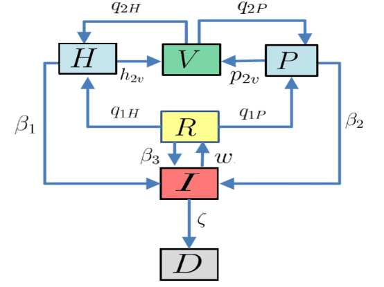
The parameters in the model characterize the infection rate of healthy agents ($\beta_{1}$), infection rate of agents with pre-existing health conditions ($\beta_{2}$), relapse rate ($\beta_{3}$), conversion rates of recovered to healthy susceptible ($q_{1H}$) and previously “immuned” to healthy susceptible ($q_{2H}$), conversion rates of recovered to pre-existing susceptible ($q_{1P}$) and previously “immuned” to pre-existing susceptible ($q_{2P}$), death rate due to non-Covid interference ($\gamma$), additional death rate due to agents with pre-existing conditions ($\delta$) and that due to infected ($\zeta$), recovery rate ($w$), rate at which healthy ($h_{2v}$) and pre-existing susceptible ($p_{2v}$) groups are quarantined. Our focus being Covid-19 infection and mortality statistics, we neglect death ($\gamma=0$) and infection rate ($\delta=0$) due to all non-Covid causes. Furthermore, data strongly suggests that $\beta_{1}\ll\beta_{2}$. Hence, the infection rate of $H$-group is considered to be a small fraction ($\lambda$) of the $P$-group, i.e. $\beta_{1}=\beta_{2}\lambda$.  The death variable $D$ thus acts like a “sink” of the dynamical system ensuring a population conservation inbuilt within the model ($H+P+I+R+V+D$ = constant).

In training our model, we find it useful to define an extra variable $I_{c}(t)$, which represents the cumulative number of those infected upto a given date. In other words, it includes not only those who are currently infected, but also those who have since recovered or died, i. e. $\frac{dI_{c}}{dt}=(\beta_{1}H +\beta_{2}P+\beta_{3}R)I.$ Since we have considered relapse in our model, it is to be noted that $I_{c}(t)\neq I(t)+R(t)+D(t)$.

Data repositories

Identifying the infection kinetics of Covid-19 as an interactive evolution process involving six time evolving population density variables: healthy susceptible ($H$), susceptible with pre-existing conditions or comorbidity ($P$), infected ($I$), recovered ($R$), naturally immuned (i.e. a clone for vaccinated $V$) and dead ($D$), the PHIRVD model uses statistics from the Johns Hopkins Covid-19 database John-Hopkins-repository to accurately predict mortality and infection statistics of 18 Asian, European and American countries. Data threshold was set beyond the first 19 days of low (or no) infection, followed by data training between 10 February 2020 to 29 June 2020. Results were later cross-verified from other databases e.g. US: https://usafacts.org; EU: https://data.europa.eu/; UK: https://coronavirus.data.gov.uk/; India: https://www.covid19india.org/. The Bayesian Markov Chain Monte Carlo (MCMC) MCMC infrastructure in PHIRVD trains the repository data to probabilistically predict the 17 parameters of the infection kinetic model (see Materials and Methods). Unlike previous predictive Machine Learning models Lancet-kucharski ; Lancet-Hellewell ; Nature-Giordano ; Science-Dehning ; Jo ; Aliou , this structure allows more dynamic adaptive control of the infection kinetic estimation resulting in a highly accurate predictive module.

Mortality and Infection: Prediction against Reality

The 18 countries or regions under study were divided into 4 infection classes, the first three based on decreasing mortality-to-infection ratio for countries past their infection peak: UK, Netherlands, Sweden, New York State (Class A); Germany, Korea, Australia, Russia, Vietnam (Class B); and Italy, Spain, Hubei (Class C). Class Class D comprises India, Poland, Iran, France, Portugal and Brazil, with ongoing infection regimes. We deliberately chose New York State instead of the entire United States due to its high population density and tourist/ worker traffic that is quite different from the national average.

(a) UK infection profiles.

(b) UK mortality profiles.

Figure 2: Infection (Fig 2a) and mortality (Fig 2b) epidemiology for the UK (Class A). Outsets represent cumulative statistics while the insets are for daily updates in the number of infected and death respectively. Here “0” marks 22 January 2020; data training between 10 February to 29 June 2020.

(a) Germany infection profiles.

(b) Germany mortality profiles.

Figure 3: Infection (Fig 3a) and mortality (Fig 3b) epidemiology for Germany (Class B). Outsets represent cumulative statistics while the insets are for daily updates in the number of infected and death respectively. Here “0” marks 22 January 2020; data training between 10 February to 29 June 2020.

(a) Italy infection profiles.

(b) Italy mortality profiles.

Figure 4: Infection (Fig 4a) and mortality (Fig 4b) epidemiology for Italy (Class C). Outsets represent cumulative statistics while the insets are for daily updates in the number of infected and death respectively. Here “0” marks 22 January 2020; data training between 10 February to 29 June 2020.

(a) India infection profiles.

(b) India mortality profiles.

Figure 5: Infection (Fig 5a) and mortality (Fig 5b) epidemiology for India (Class D). Outsets represent cumulative statistics while the insets are for daily updates in the number of infected and death respectively. Here “0” marks 22 January 2020; data training between 10 February to 29 June 2020.

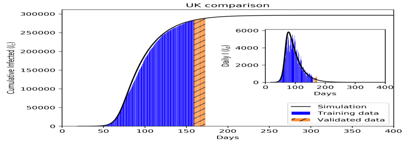
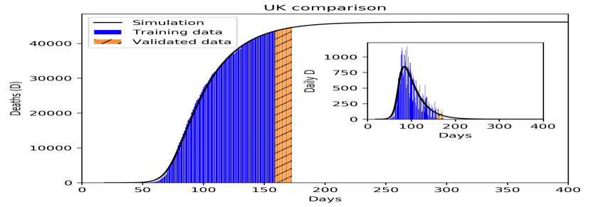
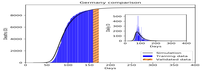
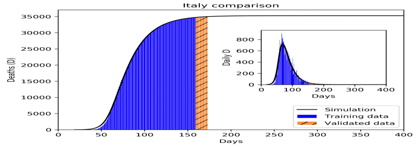
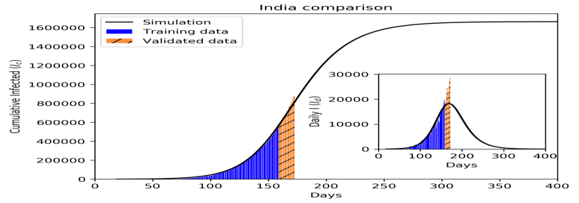
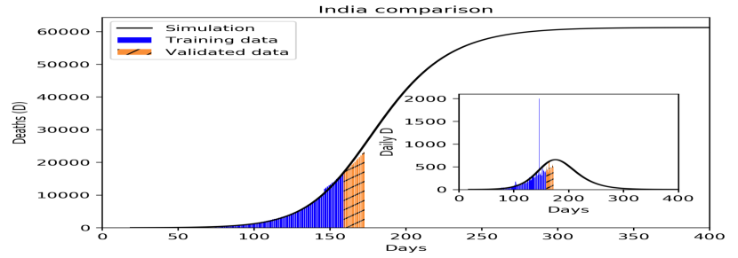
With the number of reported cases being highly dependent on the number of daily testings, not necessarily in agreement with the actual disease propagation dynamics, we observe some deviations between the simulated $I(t)$ and the actual number of reported cases. On the other hand, $D(t)$ is less affected by the testing rate. Since we are using mortality statistics with the same weightage as the infected data, we prioritize mortality prediction. We note that daily training of any epidemiological model will invariably achieve better data match, as many studies have shown, but they all lack the key predictive ability, that our ML embedded propagation kinetic model thrives on.

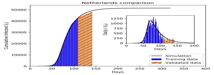
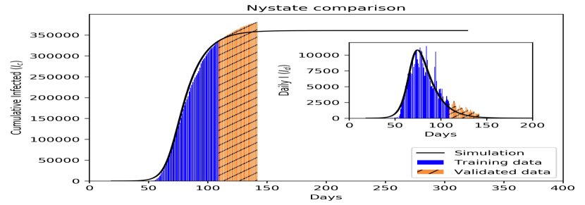
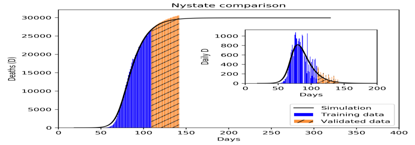
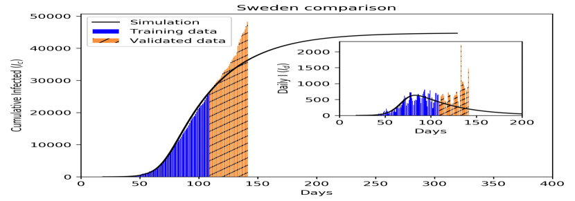
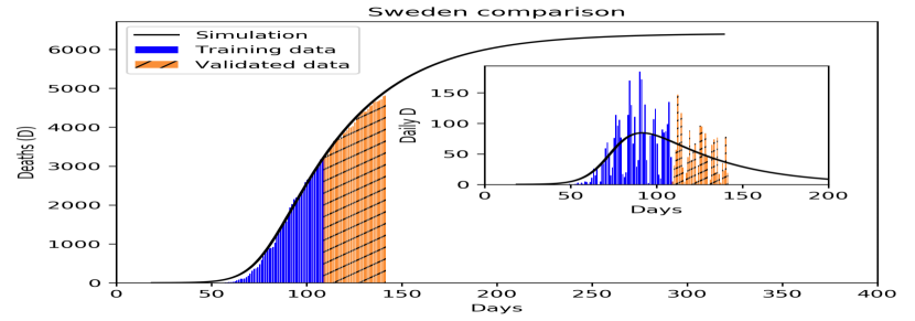
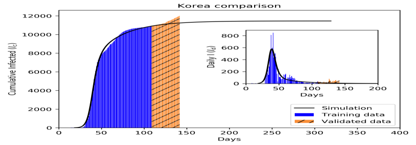
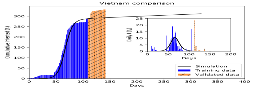
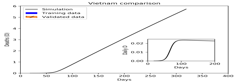
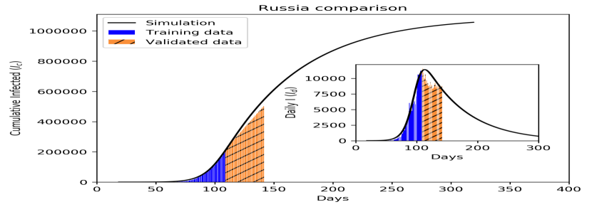
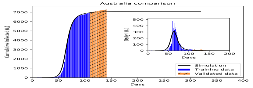
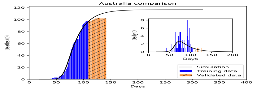
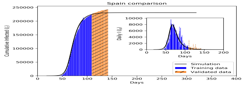
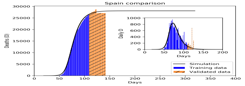
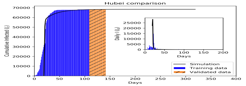
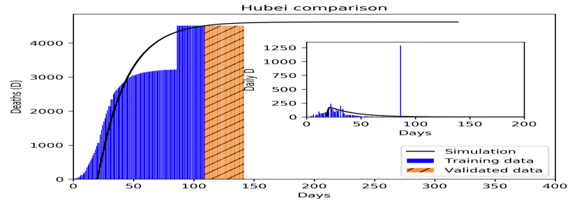
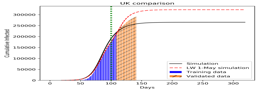
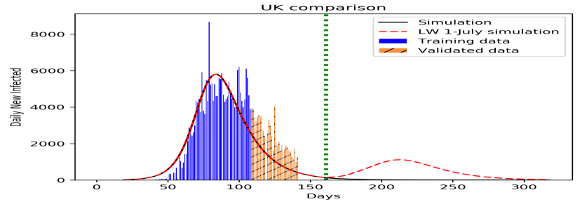
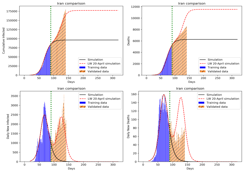
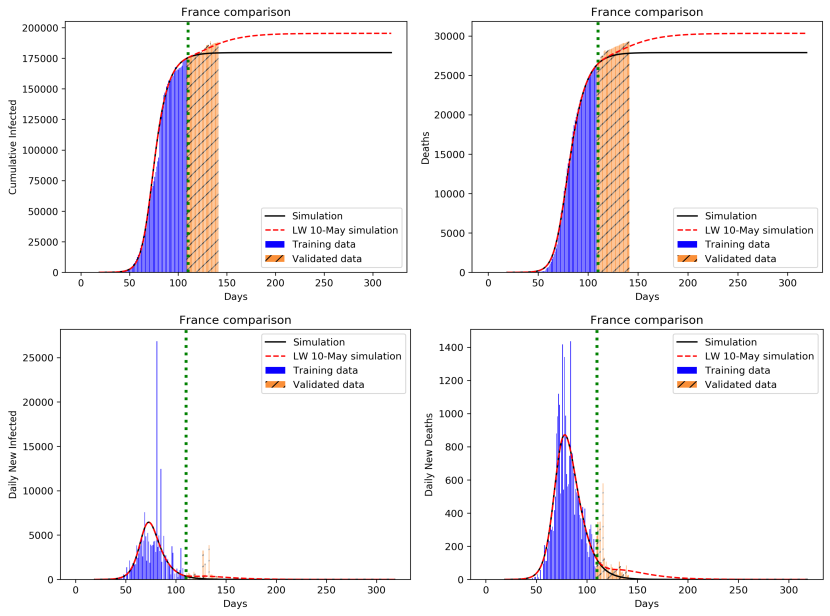
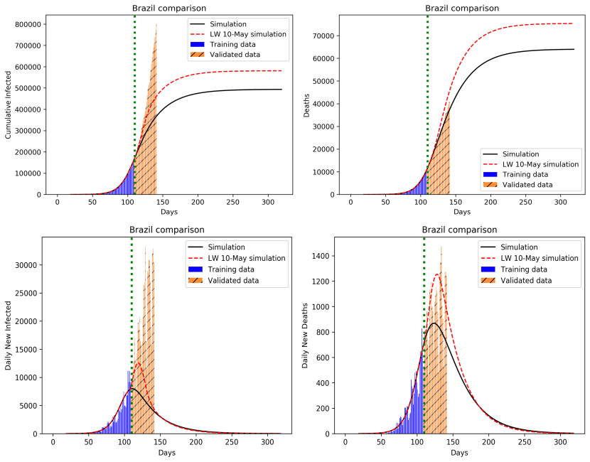
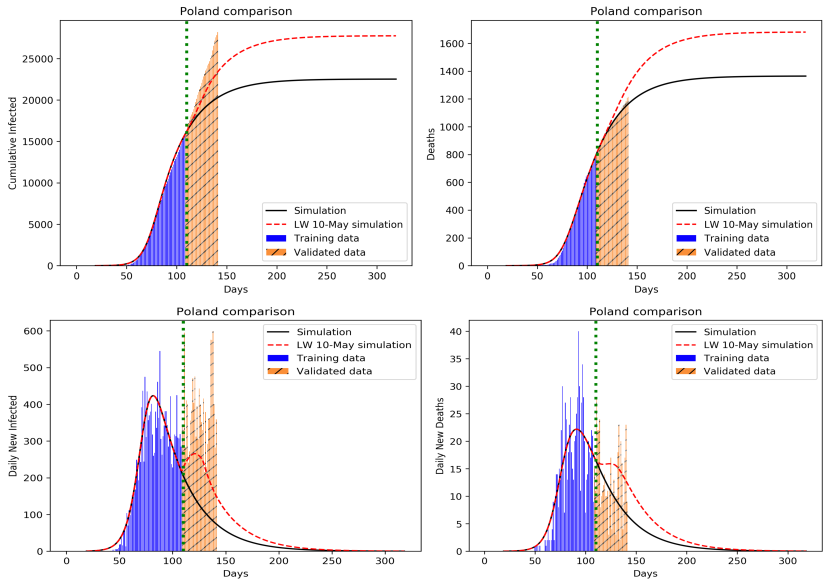
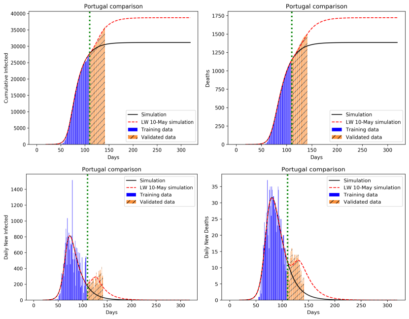
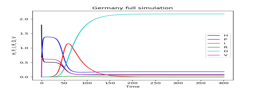
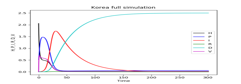
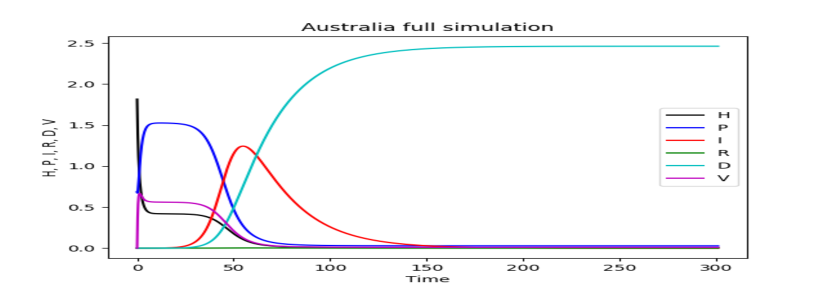
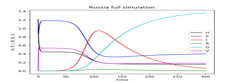
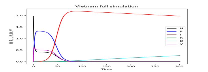
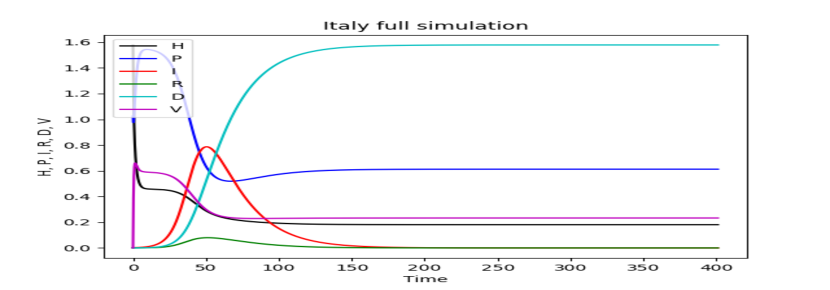
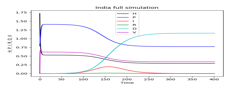
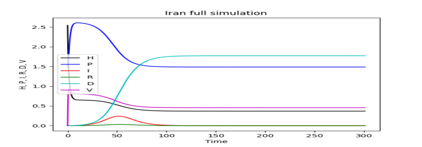
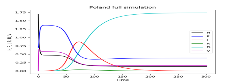
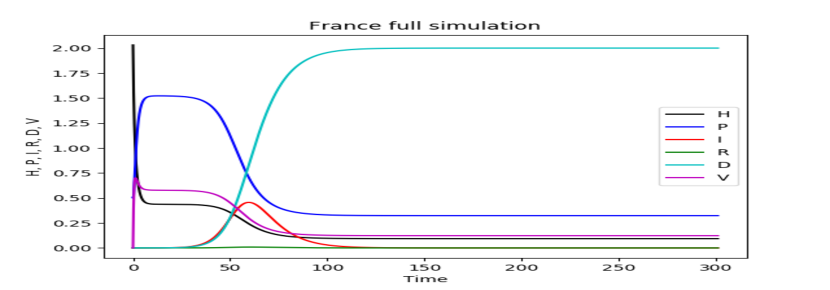
Comparative statistics for our Class A representative, the UK, is shown in Figure 2. The blue region marks the training zone that fixes the parameters. Based on the highest mortality to infection ratio in each group, the representative countries for the other 3 classes are Germany (Class B), Italy (Class C), India (Class D). Figures 3, 4 and 5 represent infection statistics for Class B (Germany), C (Italy) and D (India) respectively (other plots in Appendix II). Chi-square tested (see Materials and Methods for Chi-squared statistic used) accuracy chart in Table 1 clearly points to the veracity of the accuracy claim made. On the other hand, Vietnam presents an interesting case. With a reported zero mortality rate notwithstanding high population density, it has been repeatedly cited as an example of early quarantine success. The model tracks even such an exceptional case to a moderate level of accuracy (in Appendix II). The outsets and insets respectively outline the cumulative versus the daily infection traffic. Details for other countries, for 4 infection classes, are provided in Appendix II.

Table 2 presents a comparative chart of the PHIRVD model predictions versus real data, separately for the numbers of infected and dead, for countries representing the 4 classes with data trained between 10 February to 29 June: Class A (UK), Class B (Germany), Class C (Italy) and Class D (India). Futuristic prediction is shown until 12 July. For other countries in each individual class, with data training between 10 February to 10 May, 30 days’ prediction until 9 June establishes the predictive strength of this model (see Tables S2-S5, Appendix III), error validated as shown in Table S1 (see Appendix I).

Country	Daily New Infected		Daily New Death
	$\epsilon$	p-value	$\epsilon$	p-value
UK	0.26	0.23	0.36	0.14
Germany	0.42	0.18	0.45	0.25
Italy	0.32	0.22	0.3	0.28
India	0.52	0.25	0.52	0.38

Table 1: p-Values for daily new infected and dead for Class A-D representative countries between 11 Feb to 16 June 2020.

	UK				Germany				Italy				India
	Infected		Death		Infected		Death		Infected		Death		Infected		Death
	Data	Simulation	Data	Simulation	Data	Simulation	Data	Simulation	Data	Simulation	Data	Simulation	Data	Simulation	Data	Simulation
30/06/20	403	472	155	91	376	126	14	12	142	121	23	23	18641	17298	507	570
01/07/20	60	455	176	88	475	121	5	11	182	116	21	22	19160	17471	434	579
02/07/20	4	439	89	84	477	117	11	11	201	110	30	21	20903	17628	379	588
03/07/20	502	424	136	81	410	112	4	11	223	106	15	20	22771	17767	442	596
04/07/20	624	408	67	79	418	108	10	10	235	101	21	19	24850	17889	613	604
05/07/20	516	394	22	76	325	104	3	10	192	96	7	18	24248	17992	425	612
06/07/20	352	380	16	73	541	100	0	9	208	92	8	17	22251	18078	466	618
07/07/20	581	366	155	70	279	96	10	9	137	88	30	17	22753	18145	483	625
08/07/20	630	353	126	68	356	92	14	9	193	84	15	16	24879	18194	487	631
09/07/20	642	341	85	66	302	89	11	8	214	81	12	15	26506	18224	475	636
10/07/20	512	329	48	63	331	85	6	8	276	77	12	14	27114	18236	519	640
11/07/20	820	317	148	61	377	82	7	8	188	74	7	14	28606	18230	550	645
12/07/20	650	306	21	59	210	79	1	7	234	70	9	13	28732	18206	501	648

Table 2: Validation of Daily new Infected and Death: UK (Class A), Germany (Class B), Italy (Class C), India (Class D)

Figure 6: Daily temporal evolution of the basic reproduction rate for countries from Class A (UK), Class B (Germany), Class C (Italy) and Class D (India). The dotted line sets the pandemic threshold; count “0” starts at 14 February 2020, excluding data for the first 19 days (statistics recorded 22 January 2020 onwards) due to low infection, and additional 4 days of gestation. MCMC training between 10 February 2020 to 29 June 2020.

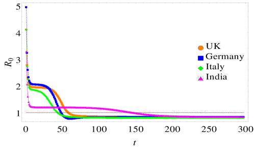
The expected number of secondary cases produced from each infected individual is traditionally defined as the basic reproduction number. A linear analytical estimation of reproduction number $R_{\text{e}}$ at fixed point leaves us with only 8 independent parameters characterizing the secondary infection kinetics (note that a linear analytical formulation does not provide an exact quantitative estimate but a proportional one only). The detailed calculation of $R_{\text{e}}$ is provided in the Materials and Methods section. Figure 6 depicts the time evolution of secondary infection for the 4 representative countries from infection classes A-D, represented by the basic reproduction number $R_{0}$ R0-Seth ; R0-Nishiura ; R0-Ferguson (see Materials and Methods). $R_{0}$ kinetics of all other countries are provided in Appendix I. Class A countries consistently show the sharpest drop in $R_{0}$ and the flattest stability period, followed by progressive decrease in $R_{0}$ decay rate and gestation span for classes B, C and D respectively. The point of note here is that while Germany and Italy show higher levels of infection than the UK, the gestation period for the UK is a lot larger than both. India shows a similar trend although the absolute numbers for India are a lot lower than the other three, indicating a complicated relationship between Full Width at Half Maximum (FWHM) and gestation period.

Discussion

Combining conventional infection kinetic modeling with a predictive Bayesian MCMC, PHIRVD quantifies the impact of lockdown as a containment tool. It precisely estimates mortality statistics for 18 countries, accurate upto the next 30 days, beyond the last date of data training. Ideal lockdown imposition and withdrawal times have been predicted and validated, including for ongoing regimen e.g. India. PHIRVD also predicts secondary relapse timings and establishes mortality-to-infection ratio as the key pandemic predictive descriptor instead of reproduction number. PHIRVD is also capable of analyzing the impact of migration, an ongoing project. Our findings clearly suggest that phased lockdown is a potent containment tool but needs to be strategically imposed, where the correct implementation and withdrawal times are paramount. Secondary infection and mortality prediction will be key to future strategic quarantine imposition and analyzing impact of future therapeutics.

PHIRVD leads to three key outcomes. First, we present highly accurate probabilistic predictions for the numbers of infected and dead for each country for a total of 18 countries, typically 3 weeks beyond the last date of (Machine Learned) data training. We can safely claim that this is the first, inherently probabilistic COVID-19 model that can claim such high levels of accuracy over such an extended time period (upto 30 days) probing in to the future and that too for all countries considered.

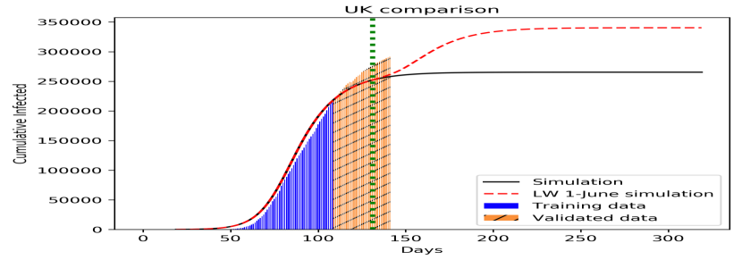
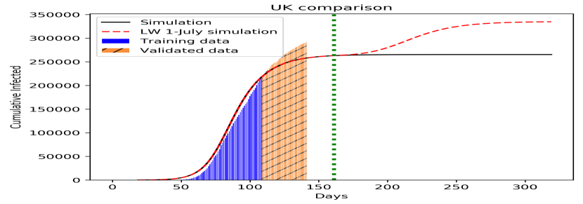
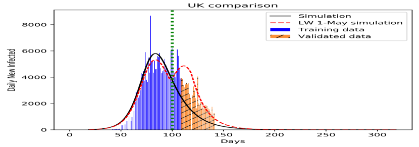
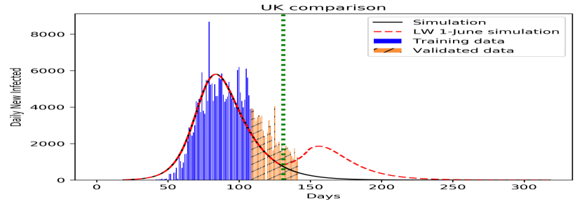
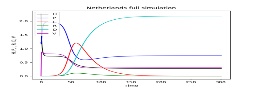
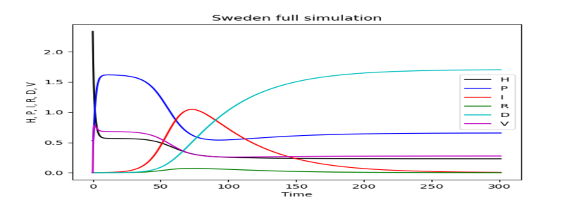
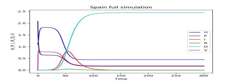
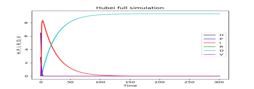
Second, we can precisely predict ideal lockdown withdrawal dates for the countries. The full simulations plots (in Appendix II) clearly outlines how an increasing infection profile initially matches with decreasing numbers of pre-existing susceptible and increasing statistics for the recovered, that then slows down as the infection peak arrives, eventually to tail off in to a no-infection landscape. While the qualitative trends are similar for all classes (A, B, C, D) of countries, the impact of lockdown on the first peak, and then a second (relapse) peak, hint at the internal health versus econometrics of the countries concerned. To prove this point, we compare infection (and mortality) propagation kinetics of 2 chosen countries for two different dates, one on the recess (UK: Figure 7), the other with uprising infection level (India: Figure 8). As opposed to the recent furore about school children being exposed to the Covid-19 menace as a result of early lockdown withdrawal, our result clearly shows that there is practically no difference in mortality between a withdrawal on June 1, 2020 as against a later withdrawal e.g. July 1, 2020 (although a withdrawal on May 1 would have been disastrous). The 1 June (almost equally safe) withdrawal would, of course, be favoured on economic and social grounds.

The third key outcome of our analysis is the establishment of mortality:infection ratio as the key descriptor of pandemic over and above reproduction number, that has conventionally been used for the purpose. The proof of this is in the accurate prediction of the secondary infection relapse time that the reproductive number fails to predict. As can be seen from Figures 7a and 7b, this relapse time period could be deferred with a late lockdown withdrawal on July 1 (as compared to June 1) although the peak mortality rates are not hugely different (ca 200 at 1 July compared to ca 400 at 1 June). Using 1 July 2020 as the UK lockdown withdrawal date, there is a clear signature of secondary relapse in the first week of September (identified as the second peak in Figure 7. The Indian situation is clearly more challenging, though, as shown in Figure 8. While perhaps economically unsustainable, India could benefit with a lockdown even beyond 31 July, 2020. For other nations like Iran, Portugal, France and Poland, our predictions of non-trivial secondary relapses (all in late June) match almost perfectly with data, both infected and dead.

(a) UK: 1 June 2020

(b) UK: 1 July 2020

Figure 7: Lockdown withdrawal dates compared for the UK (partial decclared lockdown withdrawal on 23 March 2020). Analysis is based on daily mortality statistics. The perpendicular dotted line represents lockdown withdrawal date. Here “0” marks 22 January 2020.

(a) India: 31 July 2020

(b) India: 31 August 2020

Figure 8: Lockdown withdrawal dates compared for India (partial lockdown withdrawal on 4 July 2020). Analysis is based on daily mortality statistics. The perpendicular dotted line represents lockdown withdrawal date. Here “0” marks 22 January 2020.

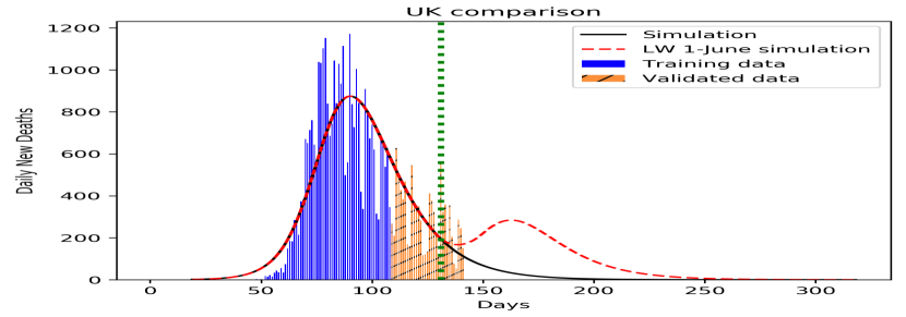
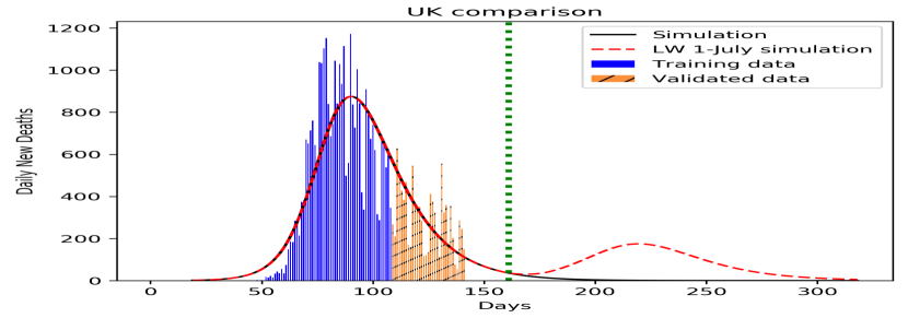
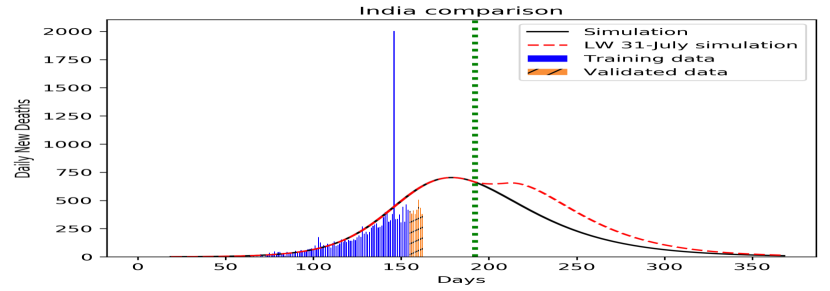
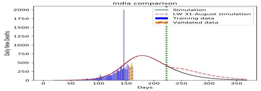
A real point of contention amongst politicians, health professionals and medical scientists has, for long, been the correct lockdown implementation and withdrawal times. In statistical parlance, this effectively amounts to an estimation of the FWHM as has been estimated for Wuhan at 2.6 weeks from initial infection Tomie . To analyze these counterclaims, we incorporate the effects of withdrawal of lockdown as a country specific, dynamically evolving quantity.

In palpable absence of any functional vaccine or therapeutics, these results can provide a remarkable gateway to pandemic strategizing, going beyond its immediate relevance. What quarantine strategy to choose and when to implement or withdraw it is of crucial importance, for which our model can serve as a future benchmark.

Materials and Methods

Motivation of the PHIRVD model

PHIRVD uniquely combines a dynamically evolving infection propagation model that tracks the phenomenology of infection kinetics with a probabilistic predictive algorithm, the latter chosen as a Bayesian Markov Chain Monte Carlo (MCMC) kernel. The Bayesian MCMC is used to train past data to predict time independent generic parameters that can predict the future statistics. The choice is guided by the strength of Bayesian MCMC in a range of dynamical modeling studies in complementary fields (32,33).

Reproduction number $R_{\text{e}}$ at fixed point

For $\gamma=0,\delta=0$, from Eq. (1) the disease free equilibrium (DFE) or fixed point is given by $P^{*}=H^{*}\frac{h_{2v}q_{2P}}{p_{2v}q_{2H}}$, $I^{*}=0,R^{*}=0$, $V^{*}=H^{*}\frac{h_{2v}}{q_{2H}}$. To evaluate the reproduction number $R_{\text{e}}$, we have to break the equation of $\frac{dI}{dt}$ into two parts $\mathcal{F},\mathcal{V}$, i.e.,

$$\frac{dI}{dt}=\mathcal{F}-\mathcal{V}$$ (2)

where $\mathcal{F}=(\beta_{1}H+\beta_{2}P+\beta_{3}R)I$ and $\mathcal{V}=(\zeta+w)I$. Now, $F=\frac{\partial\mathcal{F}}{\partial I}|_{DFE}$ and $\Sigma=\frac{\partial\mathcal{V}}{\partial I}|_{DFE}$. Then $R_{\text{e}}=\frac{F}{\Sigma}=\frac{H^{*}\left(\frac{\beta_{2}h_{2v}q_{2P}}{p_{2v}q_{2H}}+\beta_{1}\right)}{\zeta+\omega}$.

Lockdown Dynamics

During the time period, over which we trained our model, most of the countries (except Sweden), of our interest, were under lockdown. Therefore, we studied the effects of withdrawal/relaxation of lockdown for some countries by introducing a time varying parameter $L(t)$ in the model in Eq. (1) substituting $\beta_{1,2,3}$ with $\beta_{1,2,3}\>L(t)$ respectively, where $L(t)=1,\>\>\text{for}\>\>t\leq t_{0}\>\>\text{and}\>\>\alpha\>\>\text{for}\>\>t\geq t_{0}+k$. For $t_{0}<t<t_{0}+k$, $L(t)=\frac{1}{k}[\alpha(t-t_{0})+(t_{0}+k-t)]$. Here $t_{0}$ marks the lockdown withdrawal time point, $k$ is the approximate time duration during which the susceptible and infected population mixes well (e.g. within one week or one month etc.) and $\alpha$ is the parameter quantifying the homogeneity of mixing. The largest $\alpha$ value (sum of $H$, $P$, $I$, $R$, $D$ and $V$) implies that almost all susceptible have been in contact with an infected person. The function $L(t)$ is such that before lockdown withdrawal, it does not alter the contact probability while after withdrawal, it linearly increases from the value $1$ to $\alpha$ over a time interval of $k$ days, ensuring that the contact probability between susceptible and infected increases from a low to a high value within this period.

Parameter Estimation

The Bayesian MCMC data training leading to supervised learning is itself conducted in two steps using a double-filtration process. First, infection data alone are used to arrive at a preliminary set of values, characterizing each country. The said values are then filtered through combined infected and mortality statistics for a second training to sequentially converge to a preset upper limit. The training schedule is repeated multiply to ensure accurate predictions of the training dataset. Estimation of the equilibrium reproduction number is strategically used to reduce the effective parameter space from 13 to 8 parameters, perfectly conforming with the Bayesian MCMC prediction which shows that value fluctuations with other parameters do not contribute much to the infection kinetics. The model clearly separates the $H$ and $P$ infection classes to reflect their differential levels of infection and mortality. Another constituent is the death rate kinetics embedded in the central structure. The infection propagation model outlined in Eq. (1) is a multi-parameter model whose parameters are evaluated using predictive data modeling within the Bayesian MCMC construct. Similar structures have been selectively used in (19,23) albeit for single-country specific models without any explicit mortality dynamics. Over-reliance on infection statistics has often led to incorrect estimation for mortality statistics, whose accurate prediction is our first key target, an aim that is remarkably well served by our ML-embedded compartmentalised model. We present both the cumulative and daily (inset plots) statistics of infected population over $400$ days, data trained between 10 February 2020 to 29 June 2020 (140 days) and then predicted up to the next 8 weeks (shown up to 12 July 2020 in Table 1).

The Bayesian Markov Chain Monte Carlo (MCMC) algorithm:

To understand how the algorithm uses the data to determine the parameters, it is useful to recall some elements of Bayesian statistics (32, 33). Let $\bm{D}=(D_{1},D_{2},...,D_{n})$ represent the full data vector that is being used to train the algorithm. For our case, the subscripts run over both the time intervals (daily) as well as the data types, such as $I_{c}(t_{i})$ and $D(t_{i})$. Similarly, let $\bm{\Theta}=(\theta_{1},\theta_{2},...,\theta_{\alpha})$ represent the vector of parameters. A key ingredient is the prior probabibility distribution (Bayesian priors) for each $\theta_{i}$. While the absence of any knowledge of the system would call for a prior that is flat in the physically allowed region, the incorporation of such knowledge (which, in the present context, could be divined from the analysis of, say even part of the data for a single country in a given class) quickly gives the prior a somewhat peaked structure. In other words, one could as well start with a normal-distributed prior, viz., $\bm{\Theta}\sim N(\bm{\Theta_{0},\sigma})$, where the vector $\bm{\Theta_{0}}$ represents the mean of the parameters and $\bm{\sigma}=(\sigma_{1},\sigma_{2},...,\sigma_{\alpha})$ the standard deviation. As it turns out, the dependence of the final result on the prior is quite insignificant.Given a $\bm{\Theta}$, it is straightforward to calculate the conditional probability $\mathbb{P}(\bm{D|\Theta})$ of obtaining a realization $\bm{D}$ for the data. Using Bayes’ theorem, the posterior probability for $\bm{\Theta}$ given the data is expressed as

$$\mathbb{P}(\bm{\Theta}|D)=\frac{\mathbb{P}(\bm{D|\Theta})\mathbb{P}(\bm{\Theta})}{\mathbb{P}(\bm{D})},$$ (3)

where $\mathbb{P}(\bm{D)=\int_{\Omega}\mathbb{P}(\bm{D}|\bm{\Theta}})\mathbb{P}(\bm{\Theta})d\bm{\Theta}$, with $\Omega$ denoting the whole parameter space. This, immediately leads us to the likelihood ratio of two parameter vectors $\bm{\Theta_{1}}$ and $\bm{\Theta_{2}}$, namely

$$\frac{\mathbb{P}(\bm{\Theta_{2}|D})}{\mathbb{P}(\bm{\Theta_{1}|D})}=\frac{\mathbb{P}(\bm{D|\Theta_{2}})\mathbb{P}(\bm{\Theta_{2}})}{\mathbb{P}(\bm{D|\Theta_{1}})\mathbb{P}(\bm{\Theta_{1}})}\ .$$ (4)

We now resort to a 3-step algorithm:

1. Choose parameters (including initial conditions) through a random walk in the parameter space. The nature of the random walk is determined by the prior probability distributions for the parameters, including initial conditions.

2. Calculate the likelihood ratio function for the parameters, given the data.

3. Decide whether to accept the suggested parameter set or not.

Step 1:
Let $\bm{S_{i}}=(S_{i1},S_{i2},...,S_{in})$ be the simulated vector at the $i^{th}$ step for parameter values $\bm{\Theta_{i}}=(\theta_{i1},\theta_{i2},...,\theta_{i\alpha})$. Compared to the total population, the data $I_{c}(t),D(t)$ etc. are quasi-continuous and can be assumed to be drawn from a Normal distribution with respective standard deviations $\bm{\Gamma}=(\gamma_{1},\gamma_{2},...,\gamma_{n})$ and means $\bm{S_{i}}=(S_{i1},S_{i2},...,S_{in})$. Therefore, the posterior probability (or likelihood, in case of continuous probability density) of the parameter vector $\bm{\Theta_{i}}$ is,

$$\displaystyle\mathbb{P}(\bm{\Theta_{i}|D})=\frac{\mathbb{P}(\bm{D|\Theta_{i}})\mathbb{P}(\bm{\Theta_{i}})}{\mathbb{P}(\bm{D})}=(2\pi)^{-(n+\alpha)/2}\left[\prod_{j=1}^{n}\gamma_{j}\prod_{\beta=1}^{\alpha}\sigma_{\beta}\mathbb{P}(\bm{D})\right]^{-1}\,\exp\left(\frac{-1}{2}\sum_{j=1}^{n}\left(\frac{S_{ij}-D_{j}}{\gamma_{j}}\right)^{2}\right)\ .$$ (5)

Next, we execute a random walk in $\bm{\Theta}$-space with distribution $N(\bm{\Theta_{i},\sigma})$ to find $\bm{\Theta_{i+1}}$, and calculate again the posterior likelihood function, with the simulated data vector $\bm{S_{i+1}}$, corresponding to the parameter vector $\bm{\Theta_{i+1}}$ as

$$\begin{array}[]{rcl}\displaystyle\mathbb{P}(\bm{\Theta_{i+1}|D})&=&\displaystyle\frac{\mathbb{P}(\bm{D|\Theta_{i+1}})\mathbb{P}(\bm{\Theta_{i+1}})}{\mathbb{P}(\bm{D})}\\[6.88889pt] &=&\displaystyle(2\pi)^{-(n+\alpha)/2}\left[\prod_{j=1}^{n}\gamma_{j}\prod_{\beta=1}^{\alpha}\sigma_{\beta}\mathbb{P}(\bm{D})\right]^{-1}\,\exp\left(-\,\frac{1}{2}\sum_{j=1}^{n}\left(\frac{S_{(i+1)j}-D_{j}}{\gamma_{j}}\right)^{2}-\,\frac{1}{2}\sum_{\beta=1}^{\alpha}\left(\frac{\theta_{(i+1)\beta}-\theta_{i\beta}}{\sigma_{\beta}}\right)^{2}\right)\ .\end{array}$$ (6)

Step 2:
The likelihood ratio is now calculated to be $\mathbb{P}(\bm{\Theta_{i+1}|D})/\mathbb{P}(\bm{\Theta_{i}|D})$.

Step 3:
Next, we generate a uniform random number $r\sim U[0,1]$. If $r<\mathbb{P}(\bm{\Theta_{i+1}|D})/\mathbb{P}(\bm{\Theta_{i}|D})$, we accept $\bm{\Theta_{i+1}}$, otherwise we go back to Step 1 and repeat the procedure.
We have used cumulative infected and dead data as the vector $\bm{D}$ and we normalize (as described above) the data vector $\bm{D}$, as well as the simulated vector $\bm{S_{i}}$ at every step, before calculating the likelihood ratio in Step 2 above. We have used $\sigma=(\bm{\sigma_{P}},\bm{\sigma_{IC}})$, where $\bm{\sigma_{P}}=(0.01,0.01,0.01,0.01,0.01,0.01,0.01,0.01,0.01,0.01,0.01)$ only for parameters part, $\bm{\sigma_{IC}}=(0.1,0.1,0.001,0.0,0.0,0.0)$ for initial data part, and $\bm{\Gamma}=(\gamma_{1},\gamma_{2},...,\gamma_{n})$, where $\gamma_{j}=(0.1-0.05)(j-1)/(n-1)+0.05$. The initial days (where the numbers are low) in the data are given relatively smaller weightage than the later days for fitting, as the noise level is higher initially, than the signal.

Estimation of the reproduction number kinetics

Understandably, the basic reproduction number $R_{0}$ is no longer a constant. Defining $R_{0}(t)$ as the average number of secondary infections from a primary case at a given epoch $t$, and similarly $I_{d}(t)$ as the number of daily new cases, we have

$$I_{d}(t) = \int_{0}^{\infty}R_{0}(t)\leavevmode\nobreak\ I_{d}(t-\tau)\leavevmode\nobreak\ g(\tau)\leavevmode\nobreak\ d\tau,$$ (7)

where $g(\tau)$ is the probability density function of the generation time $\tau$, defined as the time required for a new secondary infection to be generated from a primary infection. In other words, $\tau$ is the time interval between the onset of a primary case to the onset of a secondary case, generated from this primary case. As is reported (26), the mean generation time is approximately $6.5$ days, we assume $g(\tau)$ has a Gamma distribution with $g(\tau)=\mathrm{Gamma}(6.5,0.62)$. We represent $R_{0}(t)$ as a function of time as

$$R_{0}(t) = \frac{I_{d}(t)}{\int_{0}^{\infty}I_{d}(t-\tau)\leavevmode\nobreak\ g(\tau)\leavevmode\nobreak\ d\tau}.$$ (8)

We approximate the denominator of equation (8) directly from our simulated data, by a discrete sum, and evaluate $R_{0}$ at $n^{th}$ day as

$$R_{0}(n) = \frac{I_{d}(t)}{\int_{0}^{\infty}I_{d}(t-\tau)\leavevmode\nobreak\ g(\tau)\leavevmode\nobreak\ d\tau}\approx\frac{I_{d}(n)}{\displaystyle\sum_{\tau=0}^{n-1}I_{d}(n-\tau)\leavevmode\nobreak\ g(\tau)}.$$ (9)

Statistical error estimation and $p$-values

Using the Chi-square statistic as $\chi^{2}\equiv\sum\limits_{i=1}^{n}\bigg{(}\frac{D_{i}-S_{i}}{\epsilon S_{i}+1}\bigg{)}^{2}$ ($0<\epsilon<1$), where $D_{i}$ are observed data and $S_{i}$ the simulated data for the $\text{i}^{\text{th}}$ day, we quantify the accuracy of our model fitting with the real data. Understandably, the data for daily new infections and daily new deaths are contaminated by noise, more severely than the corresponding cumulative data. Hence, a Chi-square test applied on cumulative data will always give a high $p$-value. However, to test the power of our predictive machine learning algorithm, we calculated the $p$-values on daily new data of deaths and infected. Assuming the real data are drawn from a normal distribution with mean value same as the simulated data, and with a standard deviation equal to some fraction of the simulated data, we derive our Chi-square statistic. Although, the real data of infected and dead are always positive, as the infection increases, this assumption is very well valid, except for a very small time interval at the starting of infection in a population.

Data and materials availability

Data from the Johns Hopkins repository (https://github.com/CSSEGISandData/Covid-19) were used, together with country specific repositories, e.g. US: https://usafacts.org; EU: https://data.europa.eu/; UK: https://coronavirus.data.gov.uk/; India: https://www.covid19india.org/. All the epidemiological information we used is documented in the Extended Data and Supplementary Tables. The codes and relevant files are made available through the Aston Data Repository.

Author Contributions

AKC and DC designed the core model, sequentially modified by SKN. SKN led the MCMC computation and model simulation, while AKC and BK led the analytical sections. DC and GG, together with SKN and BK, were in charge of comparative statistical error estimation. All authors wrote and approved the manuscript. All authors have identical contribution towards the final output.

Supporting Information Appendix (SI)

Data training: In order to establish the predictive strength of this machine Learning enforced model, in the appendices, we trained the data between 10 February to 10 May and predicted for the next 30 days (until 9 June 2020). This is uniformly done for all countries.

Appendix I: Reproduction Number Dynamics for Class A, B, C, D Countries

(a) Class A countries

(b) Class B countries and Vietnam (for comparison)

(c) Class C countries

(d) Class D countries

Figure S1: Temporal evolution of the basic reproduction rate for all 4 infection classes, on a day by day basis. The dotted line at $R_{0}=1$ points to the optimum above which the epidemic to pandemic regime starts.

Country	Daily New Infected		Daily New Death
	$\epsilon$	p-value	$\epsilon$	p-value
Australia	0.48	0.31	0.12	0.18
Korea	0.6	0.48	0.3	0.19
NY state, USA	0.55	0.24	0.45	0.17
Poland	0.45	0.67	0.25	0.28
Russia	0.55	0.14	0.25	0.19
Belgium	0.55	0.46	0.35	0.26
Brazil	0.6	0.37	0.45	0.46
Hubei	1	0	1	0
Portugal	0.5	0.17	0.19	0.69
Spain	0.75	0.19	0.5	0.87
Sweden	0.6	0.28	0.5	0.2
Vietnam	0.9	0	0.1	1
Netherlands	0.4	0.63	0.31	0.41
Iran	0.45	0.21	0.35	0.37

Table S1: p-Values for daily new infected and dead for other Class A-D countries between 10 Feb to 10 May 2020. The statistic $\chi_{D}^{2}\equiv\sum\limits_{i=1}^{n}\bigg{(}\frac{D_{i}-S_{i}}{\epsilon S_{i}+1}\bigg{)}^{2}$ ($0<\epsilon<1$) represents the chi-square value, where $D_{i}$ are observed data and $S_{i}$ the simulation data for the $\text{i}^{\text{th}}$ day.

Appendix II: Infection and mortality plots for countries in Classes A, B, C and D

(a) Netherlands infection profiles.

(b) Netherlands mortality profiles.

Figure S2: Infection (S2a) and mortality (S2b) epidemiology for Netherlands (Class A). The outsets all represent the cumulative statistics while the insets are for daily updates in the number of infected and death respectively.

(a) New York State infection profiles.

(b) New York State mortality profiles.

Figure S3: Infection (S3a) and mortality (S3b) epidemiology for New York State (Class A). The outsets all represent the cumulative statistics while the insets are for daily updates in the number of infected and death respectively.

(a) Sweden infection profiles.

(b) Sweden mortality profiles.

Figure S4: Infection (S4a) and mortality (S4b) epidemiology for Sweden (Class A). The outsets all represent the cumulative statistics while the insets are for daily updates in the number of infected and death respectively.

(a) Korea infection profiles.

(b) Korea mortality profiles.

Figure S5: Infection (S5a) and mortality (S5b) epidemiology for Korea (Class B). The outsets all represent the cumulative statistics while the insets are for daily updates in the number of infected and death respectively.

(a) Vietnam infection profiles.

(b) Vietnam mortality profiles.

Figure S6: Infection (S6a) and mortality (S6b) epidemiology for Vietnam. The outsets all represent the cumulative statistics while the insets are for daily updates in the number of infected and death respectively.

(a) Russia infection profiles.

(b) Russia mortality profiles.

Figure S7: Infection (S7a) and mortality (S7b) epidemiology for Russia (Class B). The outsets all represent the cumulative statistics while the insets are for daily updates in the number of infected and death respectively.

(a) Australia infection profiles.

(b) Australia mortality profiles.

Figure S8: Infection (S8a) and mortality (S8b) epidemiology for Australia (Class B). The outsets all represent the cumulative statistics while the insets are for daily updates in the number of infected and death respectively.

(a) Spain infection profiles.

(b) Spain mortality profiles.

Figure S9: Infection (S9a) and mortality (S9b) epidemiology for Spain (Class C). The outsets all represent the cumulative statistics while the insets are for daily updates in the number of infected and death respectively.

(a) Hubei infection profiles.

(b) Hubei mortality profiles.

Figure S10: Infection (S10a) and mortality (S10b) epidemiology for Hubei (Class C). The outsets all represent the cumulative statistics while the insets are for daily updates in the number of infected and death respectively.

(a) UK: 1 May 2020

(b) UK: 1 June 2020

(c) UK: 1 July 2020

Figure S11: UK cumulative infected prediction for 3 different withdrawal dates - 1 May 2020, 1 June 2020, 1 July 2020.

(a) UK: 1 May 2020

(b) UK: 1 June 2020

(c) UK: 1 July 2020

Figure S12: UK Lockdown prediction for 3 different withdrawal dates - 1 May 2020, 1 June 2020, 1 July 2020.

Figure S13: Iran cumulative infected and mortality prediction for lockdown withdrawal on 20 April 2020.

Figure S14: France cumulative infected and mortality prediction for lockdown withdrawal on 10 May 2020.

Figure S15: Brazil cumulative infected and mortality prediction for lockdown withdrawal on 10 May 2020.

Figure S16: Poland cumulative infected and mortality prediction for lockdown withdrawal on 10 May 2020.

Figure S17: Portugal cumulative infected and mortality prediction for lockdown withdrawal on 10 May 2020.

(a) Full simulation plots including all 6 dimensions for the UK

(b) Full simulation plots including all 6 dimensions for the Netherlands

(c) Full simulation plots including all 6 dimensions for Sweden

(d) Full simulation plots including all 6 dimensions for New York State

Figure S18: Full Simulation plots for Class A countries.

(a) Full simulation plots including all 6 dimensions for Germany

(b) Full simulation plots including all 6 dimensions for Korea

(c) Full simulation plots including all 6 dimensions for Australia

(d) Full simulation plots including all 6 dimensions for Russia

(e) Full simulation plots including all 6 dimensions for Vietnam

Figure S19: Full Simulation plots for Class B countries.

(a) Full simulation plots including all 6 dimensions for Italy

(b) Full simulation plots including all 6 dimensions for Spain

(c) Full simulation plots including all 6 dimensions for Hubei

Figure S20: Full Simulation plots for Class C countries.

(a) Full simulation plots including all 6 dimensions for India

(b) Full simulation plots including all 6 dimensions for Iran

(c) Full simulation plots including all 6 dimensions for Australia

(d) Full simulation plots including all 6 dimensions for France

(e) Full simulation plots including all 6 dimensions for Portugal

(f) Full simulation plots including all 6 dimensions for Brazil

Figure S21: Full Simulation plots for Class D countries.

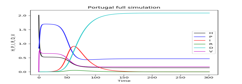
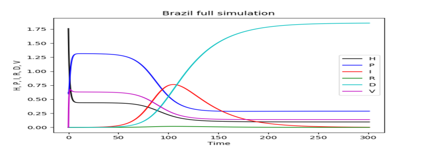
Appendix III: Comparative Estimation: Data versus Model Prediction Table

	Netherlands				Sweden				New York State, USA				Belgium
	Infected		Death		Infected		Death		Infected		Death		Infected		Death
	Data	Simulation	Data	Simulation	Data	Simulation	Data	Simulation	Data	Simulation	Data	Simulation	Data	Simulation	Data	Simulation
31/05/20	102	151	5	26	775	266	65	45	1329	395	51	51	98	144	19	45
01/06/20	86	145	10	25	2214	260	74	44	1045	368	51	48	70	138	17	43
02/06/20	209	139	13	24	1080	254	20	43	1048	343	155	45	82	132	26	41
03/06/20	210	134	15	23	1056	248	77	42	1075	319	62	42	140	126	18	39
04/06/20	183	128	6	22	948	242	17	41	1108	297	44	39	165	120	14	37
05/06/20	239	123	2	21	843	237	3	41	781	277	94	36	154	115	15	36
06/06/20	165	118	3	20	403	231	35	40	702	258	43	34	122	110	11	34
07/06/20	164	113	15	19	791	226	23	39	683	240	41	31	89	105	13	33
08/06/20	184	109	11	19	890	221	78	38	674	224	84	29	132	100	10	31
09/06/20	164	105	2	18	1474	216	19	37	736	208	38	27	142	96	7	30

Table S2: Validation of Daily new Infected and Death: Netherlands, Sweden, New York State, Belgium (Class A)

	Korea				Australia				Russia
	Infected		Death		Infected		Death		Infected		Death
	Data	Simulation	Data	Simulation	Data	Simulation	Data	Simulation	Data	Simulation	Data	Simulation
31/05/20	49	8	1	0	8	2	0	0	8858	9766	182	168
01/06/20	39	8	0	0	11	2	0	0	8529	9632	177	167
02/06/20	39	8	0	0	7	2	0	0	8823	9497	168	167
03/06/20	51	7	0	0	5	1	0	0	8718	9364	144	1660
04/06/20	57	7	0	0	7	1	0	0	8846	9231	197	165
05/06/20	38	7	0	0	6	1	0	0	8971	9100	134	164
06/06/20	38	7	1	0	2	1	0	0	8970	8970	112	163
07/06/20	50	6	2	0	7	1	0	0	8587	8841	171	162
08/06/20	45	6	0	0	11	1	0	0	8393	8714	216	161
09/06/20	56	6	1	0	4	1	0	0	8777	8588	172	159

Table S3: Validation of Daily new Infected and Death: Korea, Australia, Russia (Class B)

	Spain				Hubei Province, China
	Infected		Death		Infected		Death
	Data	Simulation	Data	Simulation	Data	Simulation	Data	Simulation
31/05/20	294	95	0	21	0	4	0	1
01/06/20	394	88	1	20	0	4	0	1
02/06/20	334	82	5	18	0	4	0	1
03/06/20	318	75	1	17	0	3	0	1
04/06/20	332	70	1	15	0	3	0	1
05/06/20	240	64	1	14	0	3	0	1
06/06/20	167	60	0	13	0	3	0	1
07/06/20	249	55	0	12	0	3	0	1
08/06/20	314	51	0	11	0	3	0	1
09/06/20	427	47	0	10	0	3	0	1

Table S4: Validation of Daily new Infected and Death: Spain, Hubei (Class C)

	Poland				Iran				Francs				Portugal				Brazil
	Infected		Death		Infected		Death		Infected		Death		Infected		Death		Infected		Death
	Data	Simulation	Data	Simulation	Data	Simulation	Data	Simulation	Data	Simulation	Data	Simulation	Data	Simulation	Data	Simulation	Data	Simulation	Data	Simulation
31/05/20	230	231	18	15	3117	2222	64	150	0	375	107	59	195	279	12	12	28936	8346	1262	1242
01/06/20	292	222	23	15	3134	2152	70	147	3856	370	81	59	366	269	11	12	28633	7777	1349	1229
02/06/20	361	213	2	15	3574	2073	59	144	0	365	43	59	331	258	8	12	30925	7269	1473	1212
03/06/20	362	204	20	14	2886	1987	63	140	552	359	46	58	377	247	10	12	30830	6815	1005	1192
04/06/20	576	196	16	14	2269	1896	75	136	529	354	31	58	382	237	9	11	27075	6409	904	1170
05/06/20	575	189	4	14	2364	1803	72	131	293	347	13	57	342	226	5	11	18912	6043	525	1146
06/06/20	599	181	9	14	2043	1707	70	126	98	341	53	56	192	216	6	11	15654	5712	679	1120
07/06/20	400	175	17	13	2095	1612	74	120	141	334	84	56	421	206	7	11	32091	5413	1272	1094
08/06/20	282	168	23	13	2011	1517	81	115	397	327	23	55	294	196	5	10	32913	5141	1274	1066
09/06/20	359	162	9	13	2218	1415	78	109	358	320	27	54	310	187	7	10	30412	4892	1239	1039

Table S5: Validation of Daily new Infected and Death: Poland, Iran, France, Portugal, Brazil (Class D)

References

- (1) N G Davies, A J Kucharski, R M Eggo, A Gimma, W J Edmunds. Effects of non-pharmaceutical interventions on COVID-19 cases, deaths, and demand for hospital services in the UK: a modelling study. The Lancet Public Health 2020; doi: https://doi.org/10.1016/S2468-2667(20)30133-X.
- (2) M Gatto, E Bertuzzo, L Mari, S Miccoli, L Carraro, R Casagrandi, and A Rinaldo. Spread and dynamics of the COVID-19 epidemic in Italy: Effects of emergency containment measures, PNAS 2020 117 (19) 10484-10491.
- (3) W C Koff, M A Wlliams. Covid-19 and Immunity in Aging Populations — A New Research Agenda, NEJM 2020; doi: 10.1056/NEJMp2006761.
- (4) J Giesecke. The invisible pandemic. The Lancet 2020; 395(10238) E98; doi:https://doi.org/10.1016/S0140-6736(20)31035-7.
- (5) M S Moghadas, C M Fitzpatrick, P Sah, A Pandey, A Shoukat, B H Singer, and A P Galvani. The implications of silent transmission for the control of COVID-19 outbreaks, PNAS 2020 117 (30) 17513-17515.
- (6) Funk S, Ciglenecki I, Tiffany A, et al. The impact of control strategies and behavioural changes on the elimination of Ebola from Lofa County, Liberia. Philos Trans R Soc Lond B Biol Sci 2017; 372: 20160302.
- (7) Thu Anh Nguyen, Quoc Cuong Nguyen, Anh Thi Kim Le, Huyen Nguyen Nguyen, Thao Thi Huong Nguyen. Modelling the impact of control measures against the Covid-19 pandemic in Vietnam. BMJ 2020: https://doi.org/10.1101/2020.04.24.20078030.
- (8) R Li et al. Substantial undocumented infection facilitates the rapid dissemination of novel coronavirus (SARS-CoV-2). Science 2020; 368(6490): 489-493.
- (9) C M Barton et al. Call for transparency of Covid-19 models. Science 2020; 368(6490): 482-483.
- (10) European Centre for Disease Prevention and Control: https://www.ecdc.europa.eu/en/cases-2019-ncov-eueea
- (11) M Ota. Will we see protection or reinfection in COVID-19? Nature Reviews Immunology 2020; 20, 351.
- (12) D Chen, et al. Recurrence of positive SARS-CoV-2 RNA in COVID-19: A case report. Int. J. Inf. Diseases 2020; 93: 297-299.
- (13) S M Kissler, C Tedijanto, E Goldstein, Y H Grad, M Lipsitch. Projecting the transmission dynamics of SARS-CoV-2 through the postpandemic period. Science 2020; 368: 860–868.
- (14) Adam J Kucharski, Timothy W Russell, Charlie Diamond, Yang Liu, John Edmunds, Sebastian Funk, Rosalind M Eggo. Early dynamics of transmission and control of Covid-19: a mathematical modelling study. Lancet Infect Dis. 2020; 20:553-58.
- (15) J W Glasser, N Hupert, M M McCauley, R Hatchett R. Modeling and public health emergency responses: lessons from SARS. Epidemics 2011; 3: 32–37.
- (16) C Fraser, S Riley, R M Anderson, N M Ferguson. Factors that make an infectious disease outbreak controllable. Proc. Natl Acad Sci USA 2004; 101: 6146–51.
- (17) C M Peak, L M Childs, Y H Grad, C O Buckee. Comparing nonpharmaceutical interventions for containing emerging epidemics. Proc. Natl Acad Sci USA 2017; 114: 4023–28.
- (18) Xi He, et al. Temporal dynamics in viral shedding and transmissibility of Covid-19. Nature Medicine 2020; 26: 672-675.
- (19) Joel Hellewell, Sam Abbott, Amy Gimma, Nikos I Bosse, Christopher I Jarvis, Timothy W Russell, James D Munday, Adam J Kucharski, W John Edmunds. Feasibility of controlling Covid-19 outbreaks by isolation of cases and contacts. Lancet Glob Health 2020; 8: e488-96.
- (20) Giulia Giordano, Franco Blanchini, Raffaele Bruno, Patrizio Colaneri, Alessandro Di Filippo, Angela Di Matteo and Marta Colaneri. Modelling the Covid-19 epidemic and implementation of population-wide interventions in Italy. Nature Medicine Letts 2020; https://doi.org/10.1038/s41591-020-0883-7.
- (21) J Denning, J Zierenberg, F PaulSpitzner, M Wibral, J Pingeiro Nato, M Wilczek, V Priesemann. Inferring change points in the spread off Covid-19 reveals the effectiveness of intervention. Science 2020: 10.1126/science.abb9789(2020)..
- (22) J T Matamalas, A Arenas, S Gómez. Effective approach to epidemic containment using link equations in complex networks. Science Advances 412, eaau4212: 10.1126/sciadv.aau4212.
- (23) H Jo, H Son, S Y Jung. Analysis of COVID-19 spread in South Korea using the SIR model with time-dependent parameters and deep learning. BMJ 2020; doi: https://doi.org/10.1101/2020.04.13.20063412.
- (24) M A Aliou, T Baldé. Fitting SIR model to COVID-19 pandemic data and comparative forecasting with machine learning. BMJ 2020; doi: https://doi.org/10.1101/2020.04.26.20081042.
- (25) John Hopkins Covid-19 repository: https://github.com/CSSEGISandData/Covid-19
- (26) A Endo, E V Leeuwen, M Baguelin. Introduction to particle Markov-chain Monte Carlo for disease dynamics modellers. Epidemics 2019; 29: 100363.
- (27) K Prem et al., The effect of control strategies to reduce social mixing on outcomes of the Covid-19 epidemic in Wuhan, China: a modelling study. The Lancet Public Health 2020 5(5): E261-E270.
- (28) E Grela, M Stich, A K Chattopadhyay. Epidemiological impact off waning immunization on a vaccinated population. Euro. Phys. J. B 2018 91: 267.
- (29) F Seth et al. Estimating the number of infections and the the impact of non-pharmaceutical interventions on COVID-19 in 11 European countries. Imperial College London 2020; doi: htttps://doi.org/10.25561/77731.
- (30) H Nishiura. Correcting the Actual Reproduction Number: A Simple Method to Estimate R0 from Early Epidemic Growth Data. Int J Environ Res Public Health 2010 Jan; 7(1): 291–302.
- (31) A Cori, N M Ferguson, C Fraser, S Cauchemez. A New Framework and Software to Estimate Time-Varying Reproduction Numbers During Epidemics. Am J Epidemiol. 2013; 178(9): 1505–1512.
- (32) T Tomie. Understanding the present status and forecasting of COVID-19in Wuhan: https://doi.org/10.1101/2020.02.13.20022251.
- (33) K Prem et al., The effect of control strategies to reduce social mixing on outcomes of the Covid-19 epidemic in Wuhan, China: a modelling study. The Lancet Public Health 2020 5(5): E261-E270.
- (34) E Grela, M Stich, A K Chattopadhyay. Epidemiological impact off waning immunization on a vaccinated population. Euro. Phys. J. B 2018 91: 267.
- (35) A. Gelman, J. B. Carlin, H. S. Stern, D. B. Dunson, A. Vehtari and D. B. Rubin. Bayesian data analysis. CRC press 2013.
- (36) J. Ramsay and G. Hooker. Dynamic data analysis. Springer 2017.