Model Dependence of Bayesian Gravitational-Wave Background Statistics for Pulsar Timing Arrays
Abstract
Pulsar timing array (PTA) searches for a gravitational-wave background (GWB) typically include time-correlated “red” noise models intrinsic to each pulsar. Using a simple simulated PTA dataset with an injected GWB signal we show that the details of the red noise models used, including the choice of amplitude priors and even which pulsars have red noise, have a striking impact on the GWB statistics, including both upper limits and estimates of the GWB amplitude. We find that the standard use of uniform priors on the red noise amplitude leads to upper limits, as calculated from one-sided Bayesian credible intervals, that are less than the injected GWB amplitude of the time. In addition, amplitude estimates of the GWB are systematically lower than the injected value by , depending on which models and priors are chosen for the intrinsic red noise. We tally the effects of model and prior choice and demonstrate how a “dropout” model, which allows flexible use of red noise models in a Bayesian approach, can improve GWB estimates throughout.
1 Introduction
Pulsar timing arrays (PTAs) are sensitive to gravitational waves (GWs) in the nanohertz frequency band (Sazhin, 1978; Detweiler, 1979; Foster & Backer, 1990). The most promising GW sources in that band are supermassive binary black holes (SMBBHs) that are formed via mergers of massive galaxies (Rosado et al., 2015). Orbiting SMBBHs can produce a gravitational-wave stochastic background (GWB), individual periodic signals, and transient GW bursts (Burke-Spolaor et al., 2018). The GWB from SMBBHs manifests in pulsar timing data as a stochastic signal that is correlated both temporally and spatially between pulsars (Hellings & Downs, 1983; Phinney, 2001; Jaffe & Backer, 2003). The spatial correlations are defined by the overlap reduction function known as the Hellings-Downs curve (Hellings & Downs, 1983), and the temporal correlations follow a steep power-law spectrum (Phinney, 2001; Jaffe & Backer, 2003)—i.e., the GWB is a spatially-correlated “red” noise process in pulsar timing data. The spatial correlations are a direct consequence of general relativity, originating from the quadrupolar nature of GWs.
However, there are also a number of potential non-GW sources of temporal correlations (red noise processes) in pulsar timing data. Intrinsic spin noise exists in many canonical pulsars (Cordes & Downs, 1985) and at a lower level in millisecond pulsars (Cordes, 2013). Clock errors and solar system ephemeris errors can manifest as spatially-correlated sources of red noise (Champion et al., 2010; Tiburzi et al., 2016). Lastly, unmodeled trends in radio-dependent propagation delays, e.g., dispersion and scattering due to the interstellar medium, will also produce red noise in pulsar timing data (Cordes & Shannon, 2010). Since the stochastic GWB is modeled as a red noise process with a steep spectral index, unmodeled or mismodeled noise in pulsars can have an impact on GWB detection statistics and parameter estimation (Hazboun et al., 2020). It is therefore imperative to accurately model the noise in individual pulsars so that it does not contaminate the GWB signal.
As PTA datasets have matured and reached astrophysically interesting levels of sensitivity, upper limits (ULs) on the amplitude of the GWB, , have been the flagship statistic quoted by PTA collaborations (Shannon et al., 2015; Lentati et al., 2016; Arzoumanian et al., 2016, 2018a). These ULs have been used to constrain model parameters for SMBBH populations (Simon & Burke-Spolaor, 2016; Arzoumanian et al., 2016), such as the relationship between SMBHs to their host galaxies, and to calculate the evidence for various SMBBH population models (Shannon et al., 2015; Sesana et al., 2018). The standard quoted is the one-sided credible interval of a Bayesian analysis and is therefore subject to the choice of the signal+noise models, including the choice of prior probability distributions for the parameters associated with these models.
1.1 Statement of the problem
In this paper, we systematically investigate how the choice of different signal+noise models, including the choice of priors, affects the estimates and ULs of the GWB returned by PTA analyses. We shall see that of utmost importance is the choice of noise model for the individual pulsars111As another pertinent example of the interplay of noise models and GWs, the development of the ECORR noise parameter (Arzoumanian et al., 2014) was in response to spurious single-source GW detections at frequencies higher than caused by noise correlated across frequencies on intraday timescales., as steep red noise in one or several pulsars can masquerade as red noise in the GWB, potentially leading to a bias in the conditional median estimate of the amplitude of the background, , or its UL, . Not surprisingly, a marginally significant GWB can be absorbed by red noise models for individual pulsars across the PTA, reducing the estimated amplitude of the GWB. It is also possible for models that do not accurately model the pulsar noise to lead to spurious increases in the estimated GWB amplitude. As shown in Hazboun et al. (2020), the significance of the detection of a GWB signal is strongly affected by which red noise models are chosen for each pulsar.
Over the years the above considerations regarding red noise led the PTA community to adopt a conservative approach that includes a red noise model for every pulsar in the array (Yardley et al., 2011; Demorest et al., 2013; Lentati et al., 2015, 2016; Arzoumanian et al., 2016, 2018a). An obvious alternative to this approach is to not model intrinsic pulsar red noise at all, which would effectively attribute any observed red noise to the GWB. This approach is arguably more conservative than the standard approach, since it results in the largest ULs on the GWB amplitude. A third choice is to allow a Bayesian analysis to choose which pulsars should include intrinsic red noise models—i.e., letting the data decide whether a red noise model for a particular pulsar is preferred to a white-noise-only model in a search for the GWB. There are a number of possibilities for implementing this more flexible pulsar noise model, including trans-dimensional models (Ellis & Cornish, 2016), hierarchical modeling (Gelman & Hill, 2007) and product space methods (Taylor et al., 2020; Carlin & Chib, 1995; Godsill, 2001; Hee et al., 2015). But for the analyses that we perform in this paper, we adopt a dropout method (Aggarwal et al., 2019) (discussed in more detail in subsection 2.1) to decide which pulsars should be assigned red noise. As we shall see below, a pulsar red noise model that utilizes the dropout method, and allows the data to decide whether or not to include intrinsic red noise in each pulsar, gives results that most robustly and accurately return the injected .
1.2 Outline of the paper
To compare the effects of different pulsar noise models on the statistics of the GWB, we analyze 400 realizations of simulated PTA data consisting of a GWB signal injected into white timing noise (WN). Details of the simulations, signal+noise models, and data analysis methods used are discussed in detail in section 2. We allow for different priors for both the amplitude of the GWB and the red noise of the individual pulsars, as well as whether or not a red noise model for a particular pulsar should be included, i.e., the dropout method. The results are described in section 3 for both GWB parameter estimation (subsection 3.1) and 95% UL calculations (subsection 3.2). It turns out that the choice of the individual red noise models has a surprisingly strong effect, especially in the case of UL analyses. We consider more realistic simulations in section 4, where we inject red timing noise for a handful of pulsars, and show that the dropout method can also handle this more realistic scenario without any problems. Finally, in section 5, we reanalyze the NANOGrav 11-year dataset using the dropout method, obtaining a revised 95% UL, . This is more than twice as large as the value reported in Arzoumanian et al. (2018a).
2 Simulated Data and Signal+Noise Models
To investigate the effect of different models and priors for the intrinsic red noise in pulsars, we performed a number of simulations and analyses. The software libstempo (Vallisneri, 2020) is used to simulate 400 realizations of a GWB with amplitude in WN at a level of for a simple PTA dataset based on the pulsars in the IPTA’s second mock data challenge (Hazboun et al., 2018). The WN is simulated using the time of arrival (TOA) errors, identical in amplitude for all pulsars. (Pulse TOAs are the fiducial data used in PTA analyses.) The amplitude of the WN is treated as a known quantity for all of the analyses. We then compare the results of the different models and priors to the results of a model that incorporates only what we know to be in the simulated data: a red GWB signal plus WN.
The construction of the likelihood and analysis methods match exactly those used in recent PTA data analysis work such as Arzoumanian et al. (2018b) and developed over the last decade in the literature (Taylor et al., 2017; Arzoumanian et al., 2016; van Haasteren & Vallisneri, 2014; Arzoumanian et al., 2014; Taylor et al., 2013; Ellis et al., 2013). Therefore, we do not describe the analysis methods in detail here except to note a few features connected to the signal+noise models relevant to this work.
The GWB is modeled as a Gaussian process (Williams & Rasmussen, 2006) in the Fourier domain (van Haasteren & Vallisneri, 2014; Lentati et al., 2016) with a power spectral density given by a power-law. The main results quoted from searches for the GWB assume a fixed spectral index for the induced timing residuals:
| (1) |
where is a reference frequency. The choice corresponds to a spectral index of for the characteristic strain of the GWB, appropriate for inspiraling binaries (Phinney, 2001; Jaffe & Backer, 2003). Typical analyses, in addition to the GWB, include a separate red noise model for each pulsar, parametrized in the same way as the GWB,
| (2) |
where both the spectral index and red noise amplitude are allowed to vary for each pulsar. This adds parameters to the search. The prior on the spectral index is taken to be uniform from to . This covers the range from white noise () to the the steepest power spectral density for which the quadratic spin down removes dependence on any lower cutoff frequency in that power spectral density (van Haasteren & Levin, 2013; Blandford et al., 1984). In principle, the prior on the spectral index could also be chosen differently (see, e.g., Callister et al. (2017)), but we do not investigate the effects of those choices here. However, we do consider the effect of different priors on the amplitudes of both the GWB and pulsar red noise, and . We use either uniform or log-uniform (uniform in log space) probability distributions for these individual amplitudes, defined over the range of values to . Table 1 lists the various signal+noise models and prior probability distributions used in our analyses. Note that in most cases the GW signal does not include Hellings-Downs spatial correlations as these considerably decrease the computational efficiency. The alternative signal model searches for a common red noise process (Arzoumanian et al., 2018a) are subscripted in Table 1 with crn.
| Model | Signal prior | Noise priors |
|---|---|---|
| GWB-only | — | |
| GWB-only | — | |
| GWB+RN | ||
| GWB+RN | ||
| GWB+RN | ||
| GWB+RN | ||
| GWB+RN | ||
All searches use the software Enterprise (Ellis et al., 2019) and enterprise_extensions for modeling the PTA data likelihood, the GWB, and the various signal+noise models. We used the Parallel Tempering Markov-Chain Monte Carlo sampler PTMCMCSampler (Ellis & van Haasteren, 2017) for sampling the likelihood.
2.1 Pulsar red noise dropout method
In addition to the two models where we only search for the GWB (GWB-only in Table 1) or where we model intrinsic red noise for every pulsar (GWB+RN in Table 1), we consider a more flexible per-pulsar noise model that uses the data to determine whether or not an individual pulsar should be modeled as having red noise (GWB+RN in Table 1). This model is implemented using the so-called dropout method (Vigeland, in prep) on the red noise model, which uses a discrete parameter to switch the red noise model for a particular pulsar on or off during the Markov Chain Monte Carlo (MCMC) sampling of a Bayesian analysis. This extremely flexible tool has been used for investigating the support of deterministic and stochastic signals in particular pulsars (Aggarwal et al., 2019, 2020). The GWB+RN analyses therefore include a red noise model for each pulsar with an amplitude and spectral index along with a dropout parameter. If the dropout parameter samples above a certain threshold, then the red noise model acts as usual. If the threshold is not met, then the red noise model is turned off completely. The threshold defines the prior odds ratio for a red noise model to be turned on.
Throughout this work we use a threshold of for the red noise model to be turned on. This means that given no support for red noise, the red noise model will be turned on only th of the time. This threshold effectively set an odds ratio of as a hurdle to overcome in order to use a red noise model for a particular pulsar. Although one can consider using different threshold values for the dropout model, we do not investigate here how these different values affect the GWB statistics.
2.2 Sensitivity to choice of priors
As discussed in subsection 1.1, the statistics derived from Bayesian analyses depend on the choice of signal+noise model, including the choice of prior probability distributions for the parameters associated with those models (Kass & Wasserman, 1996). Given sufficiently informative data the prior choices will matter little; however, PTA datasets are not yet at this point (Arzoumanian et al., 2018a). As the datasets continue to increase in duration and sensitivity increases, it is critical to understand any potential pitfalls and limitations of our analysis.
Specifically, the simulations and analyses chosen for this work allow us to compare the performance of different models, and their fidelity in returning injected GWB parameters, when applied to a relatively simple dataset. If the signal+noise model matches that used in the simulations, we should obtain, on average, the expected coverage for our credible intervals. For signal+noise models that do not match the simulations, over- or under-coverage is possible. Thus, the analyses that we perform here can be thought of as a “sensitivity analysis” (Efron, 2015), which checks the robustness of our statistical inference results to the choice of models and priors. However, these simulations do not completely test the “coverage” of different signal+noise models. Coverage is the fidelity of Bayesian credible intervals (or likewise frequentist confidence intervals) over many iterations of an analysis (Heinrich et al., 2004), which allows us to answer the question “does the injected value of a parameter fall within an interval in of simulations?” In order to formally check the coverage of a Bayesian pipeline, one would need to sample from the prior on , as well as look at different realizations, something that would be too prohibitive to do across all of the models considered here. As we shall see below, choosing the wrong model—in this case, whether or not some or all pulsars have red noise—can skew the final statistics.
3 Results of analyses on simulated data
The following two subsections describe how the choice of different signal+noise models and prior probability distributions affects both GWB parameter estimation and UL calculations.
3.1 Effect of signal+noise models on GWB parameter estimation
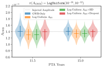
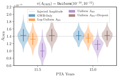
We begin by showing the effects of different signal+noise models and priors on estimates of the amplitude of the GWB. The first analysis that we performed, which serves as the base model for all comparisons, uses the GWB-only signal+noise model—i.e., we only search for the GWB and use TOAs weighted by their WN errors. Not surprisingly, given that we are analyzing the data using the same model that we used to produce the simulations, we recover posterior distributions for the median value of that agree well with the injected value, (see the blue violin plots in the two panels of Figure 1.) The two panels correspond to two different prior probability distributions for , either log-uniform or uniform over the range to . Analyses using log-uniform priors are usually referred to as “detection runs” in the PTA literature as they are especially effective for obtaining a Savage-Dickey approximation (Dickey, 1971) to the Bayes factor for weak signals. Uniform priors on the amplitude of the GWB are usually used in “upper limit” runs, in order to provide more conservative ULs on .
The other violin plots in Figure 1 show the recovered distributions of the median value of at two different observation times (11.5 and 15 years) for the other signal+noise models and priors listed in Table 1. From these recovered distributions we are able to draw several conclusions:
-
1.
As the signal to noise ratio increases the choice of prior on the signal amplitude (in this case ) has little effect on the median value of , which is expected in a Bayesian analysis. This can be seen by comparing the GWB-only and log-uniform results (blue and orange violin plots, respectively) in the two panels of Figure 1. The choice of prior on does not considerably change the distribution of median values.
-
2.
The choice of prior on has a dramatic effect on the recovery of the median value of . This can be seen by comparing the orange and purple violin plots in the right-hand panel of Figure 1. These correspond to log-uniform and uniform priors on , respectively.
-
3.
With log-uniform priors on both and , recovered median values of are systematically lower than the injected value (orange violin plots in the left-hand panel of Figure 1). This bias remains even if HD correlations are included in the signal model (green violin plots in the left-hand panel of Figure 1).
-
4.
The dropout model mitigates the effects of the prior on the posterior. It does that by including an intrinsic RN model only when it is really needed, returning results consistent with the injected amplitude of the GWB (red and brown violin plots, respectively, in the two panels of Figure 1). The difference between the brown and purple distributions shows that even uniform priors on both and return fairly accurate median values for when the dropout method is used.
While the differences in the third point above seem fairly small (i.e., the orange and green/ second and third violin plots in each set of the left-hand panel of Figure 1 are shifted lower by about ), these shifts can have fairly drastic results when considering the interpretation of a single posterior from real data. Instead of distributions of the median, one can tally the quantile position of the injected value for each of the “detection runs” (which use log-uniform priors for ). In the models where red noise is assumed for all pulsars, the injected value falls higher than a given credible interval 3 to 7 times more often than it falls lower than the same credible interval. In other words, one is 3 to 7 times more likely to underestimate than overestimate it. However, when the red noise dropout method is used, the discrepancy between the injected value falling higher or lower than the credible interval is reduced considerably, giving only a 20% difference, corresponding to a factor of 1.2.
3.2 Effect of signal+noise models on GWB upper limits
We also determine the effects of the different signal+noise models and prior distributions on the 95% UL, . For all of the UL analyses, we use the standard convention of using a uniform prior on (Lentati et al., 2016; Arzoumanian et al., 2016, 2018a). For the GWB-only signal+noise model, we recover results for consistent with expectations (see the solid blue curve in either the left or right-hand panel of Figure 2). As discussed in subsection 3.1, this is because the GWB-only signal+noise model agrees with that used to produce the simulated data. The distribution of UL values calculated for the 400 realizations of the simulated data has values that are greater than the injected value of the background roughly 93% of the time (within error of the expected value of 95%).
We then perform analyses using the standard model for PTA GWB searches which includes an intrinsic red noise model for each pulsar. Recall that these models introduce additional parameters (an amplitude, , and spectral index, , for each pulsar). To the best of our knowledge all Bayesian PTA ULs to date have used uniform priors on and . From the dashed orange curve shown in the left-hand panel of Figure 2, we see that the distribution of 95% ULs is shifted to significantly lower values, with basically even odds, i.e., 50%, that the calculated UL is above or below the injected value.
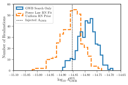
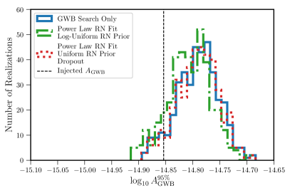
It is worth pointing out that there is nothing wrong with the ULs produced by this procedure, as long as one is explicit about the model being used in the Bayesian analysis. However, if the signal+noise model that we are using differs greatly from what gave rise to the data, then statistical inferences can be systematically (and significantly) inaccurate. The standard PTA UL analysis is based on the “conservative” assumption that all pulsars have substantial red noise. In our simulations this assumption leads to individual pulsar red noise models that are able to absorb a substantial amount of the common red process, i.e., the GWB, and thus produce an overall smaller . The effects of the “conservative” assumption can be somewhat mitigated by using instead a log-uniform prior on . This choice of prior decreases the bias, as one can see from the dot-dashed green distribution of in the right-hand plot of Figure 2, which has 87.25% of its ULs above the injected value. The log-uniform prior, however, is still part of a signal+noise model that assumes that all pulsars have at least some level of measurable red noise.
As we have already seen in subsection 3.1, a better option is to use a red noise pulsar model in conjunction with the dropout method, which allows the data to decide whether a given pulsar should be modeled to include intrinsic red noise. The dropout analysis turns off the red noise models in almost all cases for this simple simulation of GWB+WN-only, returning us to results commensurate with the GWB-only search (see the dotted red distribution in the right-hand plot of Figure 2, which has 93.25% of its ULs above the injected value). The dropout method does this by using the threshold value to effectively set a prior on the presence (or absence) of intrinsic red noise in our pulsars, allowing the data to inform the choice of noise model.
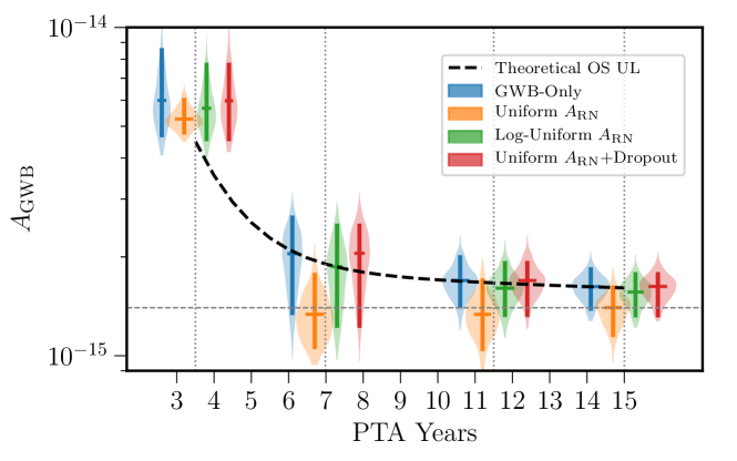
In Figure 3 we show the evolution of the UL as a function of time for the various analyses. The injected is specifically chosen so that the GWB begins to have power greater than the WN at the lowest frequencies when there is seven years of data. Before this time the ULs are all still well above the injected value, but as soon as one enters the intermediate signal regime222Defined in Siemens et al. (2013) as beginning when the power in the lowest frequency bin of the GWB is greater than that of the WN., biases in the standard GWB UL analysis (orange violin plots) are clearly manifest.
In comparison, the distributions for the dropout analysis (red violin plots) match those for the GWB-only search (blue violin plots), which also match the expected 95% confidence-level UL (black dashed line) predicted by the frequentist optimal statistic (OS) developed in Ellis et al. (2013); Siemens et al. (2013); Chamberlin et al. (2015); Vigeland et al. (2018). The scaling laws of Siemens et al. (2013) are used to construct an analytic expression for as a function of time using Equation A5. Thus, just as we saw in subsection 3.1, the pulsar red noise dropout analysis performs better than the standard PTA analysis (uniform amplitude priors for both and ) for 95% ULs as well.
4 Application to more realistic data sets
As discussed earlier, the simple simulations studied in the previous sections only included WN and a red GWB signal. For these simulations, the dropout model successfully turns off the red noise models in all pulsars, as can be seen in the top panel of Figure 4. In this panel, the vertical height of the dots shows the fraction of time the red noise dropout model is turned on for a given realization at a given slice of the dataset. A dataset that is completely ambivalent about the presence of red noise would lie along the horizontal thin dashed line, i.e., the pulsars will have their red noise model turned on th of the time, while the presence of most dots below the line shows that red noise is disfavored.

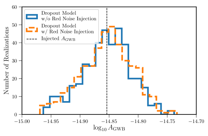
In order to assess the full abilities of the red noise dropout model, another set of simulations were run where a handful of pulsars were injected with red noise characteristic of that seen in real PTA datasets. Various amplitudes and spectral indices of red noise were injected and are detailed in the caption of Figure 4. The middle panel shows the analogous results to the top panel, but with the successful modeling of red noise in the pulsars where it has been injected. Depending on the spectral index and amplitude, it may take longer in the dataset to resolve the red noise in the pulsar, as shown by the dependence of Equation A2 on . However, for the full 15 years of data, those pulsars with injected red noise have red noise dropout models turned on through most steps of the MCMC. The bottom panel of Figure 4 shows the distribution of medians for from both dropout analyses. As one can see, the red noise dropout model does just as well at estimating whether there is red noise present in some of the pulsars or not.
5 Reassessing the NANOGrav 11-Year Analysis
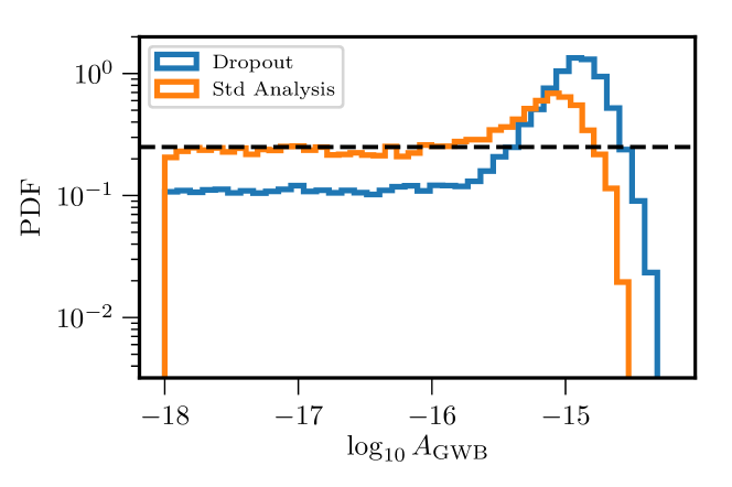
Finally we turn to real PTA data and apply the red noise dropout model to the NANOGrav 11-year dataset (Arzoumanian et al., 2018b). In addition to adding a dropout parameter for each of the pulsars, we also use the BayesEphem (Vallisneri et al., 2020) solar system ephemeris model so that our results are directly comparable to those of Arzoumanian et al. (2018a). This analysis includes the Hellings-Downs spatial correlations for the GWB. Looking at the dropout parameters in the top panel of Figure 5 we see that the analysis largely agrees with the noise analysis used in Arzoumanian et al. (2018b).

The only pulsar deemed significant in Arzoumanian et al. (2018b), where the red-noise model is turned off a majority of the time during the dropout analysis is PSR J1909–3744. Even though the red noise model for this pulsar might return uninformative posteriors for red noise when turned on in a normal analysis, it is still able to absorb power that is better described by a common signal.
The posterior on is compared to the standard PTA analysis of the Arzoumanian et al. (2018b) dataset in Figure 5. Any evidence for a detection using the dropout analysis, though slightly better, is still marginal. However, as might be expected from the analyses in subsection 3.1, the maximum a posteriori (MAP) value for using the dropout analysis is , which is larger than that from the standard analysis, , and more similar to the UL obtained in Arzoumanian et al. (2018a). We can re-weight the samples in either of the analyses (Gelman et al., 2013) shown in Figure 5 to obtain new ULs. Re-weighting the samples from the standard PTA analysis is equivalent to the log-uniform analysis discussed in subsection 3.2 and gives . If instead we re-weight the samples from the dropout analysis from Figure 5, we obtain results comparable to the dropout analysis from subsection 3.2, which appears to be the most trustworthy model examined here for obtaining ULs. This gives an UL for the NANOGrav 11-year dataset of , which is more than twice as large as the UL quoted in Arzoumanian et al. (2018a). This result is dependent on the threshold set for the dropout parameter, as discussed in subsection 2.1, and should not be taken as a concrete astrophysical result, but rather an example of how the GWB statistics can shift when using this new model. For the most up-to-date GWB results see Arzoumanian, et al., Submitted.
6 Conclusions
Here we have shown explicitly how the choice of prior on , and indeed whether pulsars have red noise models at all, can have unanticipated consequences on the statistics of . In a simulated data set with WN and a GWB, the effect of a standard GWB search with uniform priors for the pulsar intrinsic red noise amplitudes on is drastic, returning a UL lower than the injected value in about half of all realizations. As we have seen, putting a uniform prior on biases the noise model to steal power from the GWB model. The biases of other estimators, such as the conditional median, that occur for parameter estimation are smaller, but still show a consistent shift in the same direction, i.e., to smaller values of . We have implemented a simple solution to these problems—the so-called dropout method—which is a flexible red noise model for pulsars that allows the intrinsic red noise model in each pulsar to be turned off during the course of the Bayesian analysis if there is not sufficient evidence in the data to warrant its presence.
In light of the offsets in parameter estimation uncovered by this work, it is worth revisiting constraints inferred on the SMBBH population from PTA datasets. The impact of the choice of prior on the intrinsic red noise amplitudes can be seen directly by comparing the astrophysical interpretation done in NANOGrav’s 9-year GWB constraint paper (Arzoumanian et al., 2016), which used uniform priors on red noise amplitude, with that done in its 11-year GWB constraint paper (Arzoumanian et al., 2018a), which used log-uniform priors. Even though the 11-year constraint on is a smaller value, the astrophysical inference is less constraining. This is partially due to the differing models and analysis techniques. However, viewed through the lens of this work, the weakening of constraints, specifically on the relationship, were certainly impacted by the choice of prior used for the red noise amplitudes. Beyond direct constraints using , previously reported upper limits have been used in concert with electromagnetic observations to make statements about various SMBBH population models (Holgado et al., 2018; Sesana et al., 2018). Moving forward, astrophysical statements derived from past PTA constraints on will need to be more cautious in assessing the strength of their inference.
The idea that credible intervals and parameter estimation are dependent on the choice of model and priors is a common refrain in Bayesian statistics. As a result data analysts should strive to produce models and priors that robustly represent and quantify the underlying physical processes being investigated.
Appendix A Time evolution of a frequentist GWB Upper Limit
Here we derive an expression for the expected value of the frequentist 95% confidence-level UL calculated from the optimal statistic (Ellis et al., 2013; Siemens et al., 2013; Chamberlin et al., 2015; Vigeland et al., 2018). Although this is a frequentist UL, it provides a good analytic approximation to the Bayesian 95% ULs calculated in this paper.
The expected signal-to-noise ratio derived from the optimal statistic can be written in the frequency domain as (Chamberlin et al., 2015):
| (A1) |
where the indices and label the individual pulsars, is the total auto-correlated power spectral density for pulsar , is the power spectral density for the GWB, is the time span of the data, and are the overlap reduction function coefficients, here assumed to be the quadrupolar spatial correlations induced by a GWB (Hellings & Downs, 1983).
The expression for the signal-to-noise ratio can be simplified considerably for the main set of simulations considered in this work where all of the pulsars have the same level of white noise, cadence and observing time span, and there is no red noise injected into the pulsars:
| (A2) |
Here is the TOA error value for all the pulsars, is the sampling period (the cadence), and subsumes various constants333Notice the difference in minus sign of the exponent corrected from Hazboun et al. (2020).,
| (A3) |
One can relate the aforementioned scaling laws to an UL by using the complimentary error function (Allen & Romano, 1999; Hazboun et al., 2020):
| (A4) |
where is the confidence level (e.g., for a confidence-level UL), and is the effective noise level defined in terms of , , and . The expectation value of Equation A4 yields
| (A5) |
For the simple GWB+WN simulations studied in the majority of this paper, this UL is calculated analytically and plotted in Figure 3 as the dashed black line.
References
- Aggarwal et al. (2019) Aggarwal, K., Arzoumanian, Z., Baker, P. T., et al. 2019, ApJ, 880, 116, doi: 10.3847/1538-4357/ab2236
- Aggarwal et al. (2020) —. 2020, ApJ, 889, 38, doi: 10.3847/1538-4357/ab6083
- Allen & Romano (1999) Allen, B., & Romano, J. D. 1999, Physical Review D, 59, 102001, doi: 10.1103/PhysRevD.59.102001
- Arzoumanian et al. (2014) Arzoumanian, Z., Brazier, A., Burke-Spolaor, S., et al. 2014, ApJ, 794, 141, doi: 10.1088/0004-637X/794/2/141
- Arzoumanian et al. (2016) Arzoumanian, Z., Brazier, A., Burke-Spolaor, S., et al. 2016, ApJ, 821, 13
- Arzoumanian et al. (2018a) Arzoumanian, Z., Baker, P. T., Brazier, A., et al. 2018a, ApJ, 859, 47, doi: 10.3847/1538-4357/aabd3b
- Arzoumanian et al. (2018b) Arzoumanian, Z., Brazier, A., Burke-Spolaor, S., et al. 2018b, ApJS, 235, 37, doi: 10.3847/1538-4365/aab5b0
- Astropy Collaboration et al. (2018) Astropy Collaboration, Price-Whelan, A. M., Sipőcz, B. M., et al. 2018, AJ, 156, 123, doi: 10.3847/1538-3881/aabc4f
- Blandford et al. (1984) Blandford, R., Narayan, R., & Romani, R. W. 1984, Journal of Astrophysics and Astronomy, 5, 369, doi: 10.1007/BF02714466
- Burke-Spolaor et al. (2018) Burke-Spolaor, S., Taylor, S. R., Charisi, M., et al. 2018, arXiv e-prints, arXiv:1811.08826. https://arxiv.org/abs/1811.08826
- Callister et al. (2017) Callister, T., Biscoveanu, A. S., Christensen, N., et al. 2017, Phys. Rev. X, 7, 041058, doi: 10.1103/PhysRevX.7.041058
- Carlin & Chib (1995) Carlin, B. P., & Chib, S. 1995, Journal of the Royal Statistical Society. Series B (Methodological), 57, 473. http://www.jstor.org/stable/2346151
- Chamberlin et al. (2015) Chamberlin, S. J., Creighton, J. D. E., Siemens, X., et al. 2015, Phys. Rev. D, 91, 044048, doi: 10.1103/PhysRevD.91.044048
- Champion et al. (2010) Champion, D. J., Hobbs, G. B., Manchester, R. N., et al. 2010, ApJ, 720, L201, doi: 10.1088/2041-8205/720/2/L201
- Cordes (2013) Cordes, J. M. 2013, Classical and Quantum Gravity, 30, 224002. http://stacks.iop.org/0264-9381/30/i=22/a=224002
- Cordes & Downs (1985) Cordes, J. M., & Downs, G. S. 1985, ApJS, 59, 343, doi: 10.1086/191076
- Cordes & Shannon (2010) Cordes, J. M., & Shannon, R. M. 2010, arXiv e-prints, arXiv:1010.3785. https://arxiv.org/abs/1010.3785
- Demorest et al. (2013) Demorest, P. B., Ferdman, R. D., Gonzalez, M. E., et al. 2013, 762, 94, doi: 10.1088/0004-637X/762/2/94
- Detweiler (1979) Detweiler, S. 1979, ApJ, 234, 1100, doi: 10.1086/157593
- Dickey (1971) Dickey, J. M. 1971, The Annals of Mathematical Statistics, 42, 204. http://www.jstor.org/stable/2958475
- Efron (2015) Efron, B. 2015, Journal of the Royal Statistical Society. Series B (Statistical Methodology), 77, 617. http://www.jstor.org/stable/24774821
- Ellis & van Haasteren (2017) Ellis, J., & van Haasteren, R. 2017, jellis18/PTMCMCSampler: Official Release, doi: 10.5281/zenodo.1037579
- Ellis & Cornish (2016) Ellis, J. A., & Cornish, N. J. 2016, Phys. Rev. D, 93, 084048, doi: 10.1103/PhysRevD.93.084048
- Ellis et al. (2013) Ellis, J. A., Siemens, X., & van Haasteren, R. 2013, 769, 63, doi: 10.1088/0004-637X/769/1/63
- Ellis et al. (2019) Ellis, J. A., Vallisneri, M., Taylor, S. R., & Baker, P. T. 2019, ENTERPRISE: Enhanced Numerical Toolbox Enabling a Robust PulsaR Inference SuitE. http://ascl.net/1912.015
- Foster & Backer (1990) Foster, R. S., & Backer, D. C. 1990, ApJ, 361, 300, doi: 10.1086/169195
- Gelman et al. (2013) Gelman, A., Carlin, J., Stern, H., et al. 2013, Bayesian Data Analysis, Third Edition, Chapman & Hall/CRC Texts in Statistical Science (Taylor & Francis). https://books.google.com/books?id=ZXL6AQAAQBAJ
- Gelman & Hill (2007) Gelman, A., & Hill, J. 2007, Data analysis using regression and multilevel/hierarchical models, Vol. Analytical methods for social research (New York: Cambridge University Press), xxii, 625 p
- Godsill (2001) Godsill, S. J. 2001, Journal of Computational and Graphical Statistics, 10, 230. http://www.jstor.org/stable/1391010
- Hazboun et al. (2018) Hazboun, J. S., Mingarelli, C. M. F., & Lee, K. 2018, arXiv e-prints, arXiv:1810.10527. https://arxiv.org/abs/1810.10527
- Hazboun et al. (2020) Hazboun, J. S., Simon, J., Taylor, S. R., et al. 2020, ApJ, 890, 108, doi: 10.3847/1538-4357/ab68db
- Hee et al. (2015) Hee, S., Handley, W. J., Hobson, M. P., & Lasenby, A. N. 2015, Monthly Notices of the Royal Astronomical Society, 455, 2461, doi: 10.1093/mnras/stv2217
- Heinrich et al. (2004) Heinrich, J., Blocker, C., Conway, J., et al. 2004, arXiv e-prints, physics/0409129. https://arxiv.org/abs/physics/0409129
- Hellings & Downs (1983) Hellings, R. W., & Downs, G. S. 1983, 265, L39, doi: 10.1086/183954
- Hobbs & Edwards (2012) Hobbs, G., & Edwards, R. 2012, Tempo2: Pulsar Timing Package. http://ascl.net/1210.015
- Holgado et al. (2018) Holgado, A. M., Sesana, A., Sandrinelli, A., et al. 2018, MNRAS, 481, L74, doi: 10.1093/mnrasl/sly158
- Jaffe & Backer (2003) Jaffe, A. H., & Backer, D. C. 2003, Astrophysical Journal, 583, 616, doi: 10.1086/345443
- Kass & Wasserman (1996) Kass, R. E., & Wasserman, L. 1996, Journal of the American Statistical Association, 91, 1343, doi: 10.1080/01621459.1996.10477003
- Lentati et al. (2015) Lentati, L., Taylor, S. R., Mingarelli, C. M. F., et al. 2015, MNRAS, 453, 2576, doi: 10.1093/mnras/stv1538
- Lentati et al. (2016) Lentati, L., et al. 2016, Mon. Not. Roy. Astron. Soc., 458, 2161, doi: 10.1093/mnras/stw395
- Phinney (2001) Phinney, E. S. 2001, ArXiv Astrophysics e-prints
- Rosado et al. (2015) Rosado, P. A., Sesana, A., & Gair, J. 2015, MNRAS, 451, 2417, doi: 10.1093/mnras/stv1098
- Sazhin (1978) Sazhin, M. V. 1978, Soviet Ast., 22, 36
- Sesana et al. (2018) Sesana, A., Haiman, Z., Kocsis, B., & Kelley, L. Z. 2018, ApJ, 856, 42, doi: 10.3847/1538-4357/aaad0f
- Shannon et al. (2015) Shannon, R. M., Ravi, V., Lentati, L. T., et al. 2015, Science, 349, 1522, doi: 10.1126/science.aab1910
- Siemens et al. (2013) Siemens, X., Ellis, J., Jenet, F., & Romano, J. D. 2013, Classical and Quantum Gravity, 30, 224015. http://stacks.iop.org/0264-9381/30/i=22/a=224015
- Simon & Burke-Spolaor (2016) Simon, J., & Burke-Spolaor, S. 2016, ApJ, 826, 11, doi: 10.3847/0004-637X/826/1/11
- Taylor et al. (2013) Taylor, S. R., Gair, J. R., & Lentati, L. 2013, Phys. Rev. D, 87, 044035, doi: 10.1103/PhysRevD.87.044035
- Taylor et al. (2017) Taylor, S. R., Lentati, L., Babak, S., et al. 2017, Phys. Rev. D, 95, 042002, doi: 10.1103/PhysRevD.95.042002
- Taylor et al. (2020) Taylor, S. R., van Haasteren, R., & Sesana, A. 2020, arXiv e-prints, arXiv:2006.04810. https://arxiv.org/abs/2006.04810
- Tiburzi et al. (2016) Tiburzi, C., Hobbs, G., Kerr, M., et al. 2016, MNRAS, 455, 4339, doi: 10.1093/mnras/stv2143
- Vallisneri (2020) Vallisneri, M. 2020, libstempo: Python wrapper for Tempo2. http://ascl.net/2002.017
- Vallisneri et al. (2020) Vallisneri, M., Taylor, S. R., Simon, J., et al. 2020, ApJ, 893, 112, doi: 10.3847/1538-4357/ab7b67
- van Haasteren & Levin (2013) van Haasteren, R., & Levin, Y. 2013, Mon. Not. Roy. Astron. Soc., 428, 1147, doi: 10.1093/mnras/sts097
- van Haasteren & Vallisneri (2014) van Haasteren, R., & Vallisneri, M. 2014, Phys. Rev. D, 90, 104012, doi: 10.1103/PhysRevD.90.104012
- Vigeland et al. (2018) Vigeland, S. J., Islo, K., Taylor, S. R., & Ellis, J. A. 2018, Phys. Rev. D, 98, 044003, doi: 10.1103/PhysRevD.98.044003
- Williams & Rasmussen (2006) Williams, C. K., & Rasmussen, C. E. 2006, the MIT Press, 2, 4
- Yardley et al. (2011) Yardley, D. R. B., Coles, W. A., Hobbs, G. B., et al. 2011, MNRAS, 414, 1777, doi: 10.1111/j.1365-2966.2011.18517.x