The phase diagram of the multi-matrix model with $ABAB$ interaction from functional renormalization

Abstract

At criticality, discrete quantum-gravity models are expected to give rise to continuum spacetime. Recent progress has established the functional renormalization group method in the context of such models as a practical tool to study their critical properties and to chart their phase diagrams. Here, we apply these techniques to the multi-matrix model with $ABAB$ interaction potentially relevant for Lorentzian quantum gravity in 3 dimensions. We characterize the fixed-point structure and phase diagram of this model, paving the way for functional RG studies of more general multi-matrix or tensor models encoding causality and subjecting the technique to another strong test of its performance in discrete quantum gravity by comparing to known results.

1 Introduction

Understanding the quantum properties of spacetime is a fascinating challenge. A variety of approaches is currently being explored concertedly; more recently with an increased interest in understanding relations between different perspectives. The matrix/tensor model approach DiFrancesco:1993cyw ; Gurau:2016cjo ; gurau2017random ; Rivasseau:2016wvy ; Delporte:2018iyf is located at a particular vantage point within this “landscape” of theories, with potential links to a number of different ones: Firstly, its origin in two-dimensional gravity is closely linked to string theory. Secondly, its generalization to higher dimensions is closely connected to a model that is being explored in the context of the AdS/CFT conjecture Witten:2016iux ; Rosenhaus:2019mfr . Thirdly, in matrix models a tentative connection to an asymptotically safe fixed point in the vicinity of two dimensions has been found Eichhorn:2014xaa and conjectured in higher dimensions Eichhorn:2019hsa . Fourth, this class of models provides a combinatorial approach to dynamical triangulations, complementing computer simulations of the latter Ambjorn:2001cv ; Ambjorn:2012jv ; Loll:2019rdj . This rich set of connections motivates a joint study of matrix and tensor models and in particular the search for a universal continuum limit in these. Functional Renormalization Group techniques have been developed for these models Eichhorn:2013isa ; Eichhorn:2014xaa ; Eichhorn:2017xhy and are being applied in Eichhorn:2018ylk ; Eichhorn:2018phj ; Lahoche:2019ocf ; Eichhorn:2019hsa and related tensorial group field theories Benedetti:2014qsa ; Benedetti:2015yaa ; Geloun:2015qfa ; Geloun:2016qyb ; Carrozza:2016tih ; Lahoche:2016xiq ; Lahoche:2018vun ; Lahoche:2018oeo ; BenGeloun:2018ekd ; Lahoche:2019orv ; Baloitcha:2020idd ; Pithis:2020sxm ; Pithis:2020kio , with the potential to discover a universal continuum limit beyond perturbation theory, see also Krajewski:2015clk ; Krajewski:2016svb for related developments with the Polchinski equation.
To set the stage for our studies, we first provide a more in-depth overview of the relevant quantum-gravity approaches.

The above approaches center on the path integral

$$Z=\int\mathcal{D}g\leavevmode\nobreak\ \text{e}^{iS[g]}\,,$$ (1)

where the integration runs over all field histories, given by spacetime metrics $g$ of the $d$-dimensional manifold $\mathcal{M}$ up to diffeomorphisms thereof at fixed spacetime topology. Working with the Einstein-Hilbert action, one can make sense of the weak-field limit in an effective-field theory framework Donoghue:2012zc , but encounters perturbative non-renormalizability, resulting in a loss of predictivity, beyond tHooft:1974toh ; Goroff:1985th . A possible way out of this issue is to replace the Einstein-Hilbert action by one which allows for a unitary and perturbatively renormalizable QFT. However, this might dispense with micro-causality as in the case of higher-derivative gravity PhysRevD.16.953 ; Donoghue:2019ecz ; Donoghue:2019fcb or with Lorentz invariance as in Hořava-Lifshitz gravity Horava:2009uw , see Steinwachs:2020jkj for a recent review.

An alternative pathway to quantize gravity within the continuum formulation of the path integral is explored by the asymptotic-safety program. To sidestep the problems of the perturbative quantization, this approach is based on an interacting fixed point in the Renormalization Group (RG) flow for gravity in the UV weinberg1978critical ; weinberg1979ultraviolet ; Reuter:1996cp . If it exists, such a fixed point provides a well-defined continuum limit to the path integral. At the same time, it generalizes perturbative renormalizability by ensuring that the low-energy limit is parameterized by only a finite set of free parameters, namely the relevant directions of the fixed point. There are several techniques suitable to explore asymptotic safety in gravity, falling into the two broad categories of lattice approaches and continuum approaches. A much used method pioneered for gravity by Reuter Reuter:1996cp is provided by the functional Renormalization Group (FRG) Wetterich:1992yh ; Morris:1993qb , see Dupuis:2020fhh for a review. At its core lies the implementation of the Wilsonian idea of a coarse graining operation which progressively eliminates short scale fluctuations. Indeed, all explicit calculations within truncated RG flows find evidence for the existence of such a fixed point, defining the Reuter universality class, providing compelling indications for asymptotic safety in Euclidean gravity, see, e.g., Percacci:2017fkn ; Eichhorn:2018yfc ; reuter2018quantum ; Pereira:2019dbn ; Reichert:2020mja ; Bonanno:2020bil ; Eichhorn:2020mte for recent reviews and introductions. Rephrased in a lattice-like language, such a universality class enables one to take a universal continuum limit.
Open questions in this approach have been discussed in Donoghue:2019clr ; Bonanno:2020bil and include the fate of background independence, given the assumption of an auxiliary background metric therein Reuter:1996cp ; Becker:2014qya ; Falls:2020tmj . Moreover, since the signature of the setup is Euclidean and one can in general not expect the Wick rotation to exist in a quantum gravitational context Demmel:2015zfa ; Visser:2017atf ; Baldazzi:2018mtl ; Baldazzi:2019kim , it is open how to relate these results and in particular the feature of asymptotic safety to Lorentzian quantum gravity; for a first step in this direction see Manrique:2011jc . Similarly to the characterization of other interacting fixed points, a concerted use of several different techniques could in the future provide a qualitatively and quantitatively robust grasp of the fixed point and its properties. In the case of quantum gravity, background-independent, Lorentzian approaches to quantum gravity are of particular interest to explore as techniques that can complement the FRG results.

One such promising approach to evaluate the path integral over geometries, possibly extended by a sum over topologies, and to discover a universal continuum limit, a.k.a. asymptotic safety, is by means of a sum over discrete triangulations, together with exchanging the continuum action with its discretized reformulation. In spite of the physical discreteness that some of these settings exhibit, such as, e.g., Loop Quantum Gravity Rovelli:1987df ; Rovelli:1989za ; Thiemann:2007pyv , taking a universal continuum limit is a central goal also in this setting. For instance, in group field theory Freidel:2005qe ; Oriti:2006se ; Carrozza:2016vsq ; Pithis:2019tvp , promising results regarding asymptotic freedom BenGeloun:2012pu ; BenGeloun:2012yk and asymptotic safety Carrozza:2014rya ; Carrozza:2016tih have been obtained, see Carrozza:2016vsq for a review. Similarly, RG techniques are being developed and applied in the search for a critical point in spin foams, see Dittrich:2014ala ; Steinhaus:2020lgb . In this setting, studies of the phase diagram of quantum gravity have only recently started Delcamp:2016dqo ; Bahr:2016hwc ; Steinhaus:2018aav ; Bahr:2018gwf . In contrast, in the Euclidean and Causal Dynamical Triangulation approaches (EDT, CDT) Loll:1998aj ; Ambjorn:2012jv ; Ambjorn:2013tki ; Loll:2019rdj , much is already known about the phase diagram. Going beyond two dimensions, early numerical studies using Monte-Carlo methods Ambjorn:1991pq ; Agishtein:1991cv ; Catterall:1994pg ; Bilke:1996ek have only recovered unphysical geometries Bialas:1996wu ; deBakker:1996zx ; Catterall:1996gj in the Euclidean setting, though the inclusion of additional terms in the action or measure of the path integral, associated with additional tunable parameters, might change the situation Laiho:2016nlp ; Ambjorn:2013eha . It is argued that these pathological configurations are the result of topology change leading to spaces called branched polymers which are built from one-dimensional branched-out filaments Ambjorn:1993sy ; Ambjorn:1995dj ; Bialas:1996wu ; Catterall:1994pg . At the classical level, as long as Morse geometries are excluded Sorkin:1997gi ; Dowker:1997hj ; Borde:1999md , it is long known that topology change leads to a degenerate local light cone structure and thus to a violation of micro-causality Geroch:1967fs . Thus, in the CDT approach discrete spacetime configurations with spatial topology change are excluded Ambjorn:1998xu . This leads to a much better behaved theory with the potential to produce a phase with physically relevant, i.e., extended macroscopic geometries Ambjorn:2012jv ; Ambjorn:2013tki ; Loll:2019rdj , bordered by a second-order phase transition Ambjorn:2011cg ; Ambjorn:2012ij ; Ambjorn:2016mnn ; Ambjorn:2020azq that enables a continuum limit. Yet, a key challenge in the numerical approach to dynamical triangulations remains to follow RG trajectories towards the continuum limit Ambjorn:2014gsa and calculate the scaling spectra to determine and characterize the universality class.

Matrix DiFrancesco:1993cyw and tensor models Gurau:2016cjo ; gurau2017random ; Rivasseau:2016wvy ; Delporte:2018iyf sit at a confluence of several of these approaches. They encode random discrete geometries in dimensions $d\geq 2$. Their general idea is to represent $d-1$ simplices corresponding to building blocks of geometry as rank $d$-tensors. The tensor action encodes how to glue these building blocks together to construct $d$-dimensional discrete geometries. These correspond to the Feynman diagrams in the perturbative expansion of the tensor path integral. This establishes a duality between tensor models and the discrete gravitational path integral. Indeed, in their simplest form matrix and tensor models can be understood as generators of EDTs. However, apart from the case in $d=2$ DiFrancesco:1993cyw , their continuum limit so far only leads to geometrically degenerate configurations Gurau:2016cjo ; gurau2017random , the same way as in EDT, or planar ones Lionni:2017xvn . Recent results indicate the possibility for non-trivial universality classes Eichhorn:2018ylk ; Eichhorn:2019hsa ; however, the geometric properties of the corresponding phases have not been investigated yet. If a universal continuum limit within a phase with desirable geometric properties can be taken, asymptotic safety can be confirmed in a background-independent fashion and with straightforward access to the scaling exponents. Thus, the critical role of universality in these models has been emphasized in Rivasseau:2011hm ; Eichhorn:2018phj .
Yet, in studies beyond two dimensions, the inclusion of causality has remained an open question – similarly as in the continuum approach to asymptotic safety. The success of CDT may be taken as a hint to consider additional structure enforcing micro-causality to recover higher-dimensional physical continuum geometries from such models. This idea has already been implemented in the context of matrix models for $2d$ quantum gravity, giving rise to a description equivalent to CDT in $(1+1)$ dimensions Benedetti:2008hc . In order to explore the impact of Lorentzian signature in higher dimensions, one could naturally try to impose such causality conditions on a model for tensors of rank $d\geq 3$. Yet, there already exists a proposed correspondence between a multi-matrix model with CDT in $2+1$ dimensions Ambjorn:2001br . More precisely, it corresponds to a Hermitian two-matrix model with $ABAB$ interaction which also has intimate connections to vertex-models of statistical physics ZinnJustin:2003kq ; Kazakov:1998qw ; ZinnJustin:1999wt ; Kostov:1999qx . It leads to a variant of CDT defined on an enlarged ensemble of configurations which also allows for specific degeneracies of the local geometry, dubbed “wormholes” in the literature Ambjorn:2001br . The purpose of this article is to chart the phase structure of this matrix model and in particular to study its continuum limits by means of the FRG methodology. The application of the FRG in the discrete quantum gravity context facilitates a background-independent form of coarse graining where the number of degrees of freedom serves as a scale for a Renormalization Group flow. This program was started by analyzing matrix models for $2d$ Euclidean quantum gravity in Eichhorn:2013isa ; Eichhorn:2014xaa and has by now been extended to tensor models for Euclidean quantum gravity in $3$ and $4$ dimensions Geloun:2016xep ; Eichhorn:2017xhy ; Eichhorn:2018ylk ; Eichhorn:2019hsa , see Eichhorn:2018phj for a review. Related developments for non-commutative geometry Sfondrini:2010zm ; perezsanchez2020multimatrix and tensorial group field theories Benedetti:2014qsa ; Benedetti:2015yaa ; Geloun:2015qfa ; Geloun:2016qyb ; Carrozza:2016tih ; Lahoche:2016xiq ; Lahoche:2018vun ; Lahoche:2018oeo ; BenGeloun:2018ekd ; Lahoche:2019orv ; Baloitcha:2020idd ; Pithis:2020sxm ; Pithis:2020kio exist. Recently, a first FRG analysis of the above-mentioned causal matrix model for CDT in $1+1$ dimensions has been completed CMMFRG .

The article is organized as follows: In Sec. 2 we discuss causality in the matrix-model context and review the relation of the $ABAB$ matrix model to CDTs, following Refs. Ambjorn:2001br ; Ambjorn:2003sr ; Ambjorn:2003ct . In Sec. 3, we briefly review functional RG techniques and apply them to the $ABAB$ matrix model. We then present results for the phase diagram and fixed-point structure. In Sec. 4 we review what is known about the phase diagram in the literature Ambjorn:2001br ; Ambjorn:2003sr ; Ambjorn:2003ct ; Kazakov:1998qw ; ZinnJustin:2003kq and compare our results to it. Finally, in Sec. 5 we discuss implications of our results and future directions.

2 Causality and matrix models

Spacetime is rather distinct from space, both at the conceptual as well as mathematical level. Therefore, it is crucial to take this difference into account in quantum gravity, with the distinct phase diagrams of CDT and EDT constituting a clear example of the impact of causality. In the matrix and tensor model approach, the additional structure imposed on discrete configurations by causality can be implemented through additional degrees of freedom: In Refs. Benedetti:2008hc ; CMMFRG , this is done by an external matrix, whereas the $ABAB$ model uses two dynamical matrices to generate configurations which carry imprints of causality. This strongly motivates the further development of FRG techniques for multi-matrix/tensor settings, such that similar developments can be made possible in higher dimensions.
In this section, we will review the relation of the $ABAB$ matrix model to 2+1 dimensional discrete spacetime configurations. In particular, we will follow Refs. Ambjorn:2001br ; Ambjorn:2003sr ; Ambjorn:2003ct to also review the connection to CDT.

The $ABAB$ matrix model is defined by the following partition function

$$Z[J_{A},J_{B}] = \int\text{d}A\,\text{d}B\,{\rm exp}\Big{(}-\frac{1}{2}\mathrm{Tr}\left(AA\right)-\frac{1}{2}\mathrm{Tr}\left(BB\right)+\frac{\bar{\alpha}_{1}}{4}\mathrm{Tr}\left(AAAA\right)+\frac{\bar{\alpha}_{2}}{4}\mathrm{Tr}\left(BBBB\right)$$ (2)

$$+\frac{\bar{\beta}}{2}\mathrm{Tr}\left(ABAB\right)+\mathrm{Tr}\left(J_{A}A\right)+\mathrm{Tr}\left(J_{B}B\right)\Big{)},$$

where $A$ and $B$ are Hermitian $N^{\prime}\times N^{\prime}$ matrices and $J_{A}$ and $J_{B}$ are the respective external ($N^{\prime}\times N^{\prime}$-matrix) sources. Its Feynman diagrams are ribbon diagrams with two distinct types of lines; such that the duals of the three types of vertices correspond to three distinct squares, cf. Fig. 1. This already highlights that the model reduces to the standard two-dimensional gravity case, when $\bar{\beta}\rightarrow 0$. In the presence of $\bar{\beta}$, 2+1 dimensional structure can be encoded Ambjorn:2001br .

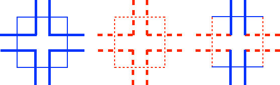
Figure 1: Distinct squares correspond to blue/continuous (type $A^{4}$), red/dashed (type $B^{4}$) and bi-colored/continuous-dashed (type $ABAB$) $4$-vertices in the dual ribbon/fat graph generated by the matrix model.

In CDTs, one only considers geometries with Lorentzian signature which admit a global foliation in proper time $t$ and disallow topology change such that micro-causality is rigidly maintained. The basic building blocks are pyramids and tetrahedra with distinct timelike and spacelike edges, of which three distinct types make up the discrete configuration, cf. Fig. 2, see also Refs. Ambjorn:2000dja ; Ambjorn:2001br ; Kazakov:1989bc ; Ambjorn:2000dv . The correspondence with the ribbon graphs of the $ABAB$ matrix model arises when considering the spatial hypersurface at $t+a/2$, also indicated in Fig. 2, where the three distinct types of squares dual to the vertices of the matrix model, cf. Fig. 1, appear. In the $t+a/2$ spatial planes, quadrangulations are formed as, e.g., in Fig. 3, the duals of which are the ribbon graphs of the matrix model. This already suggests that any CDT configuration can be encoded in terms of a Feynman diagram of the matrix model, which would motivate setting the CDT partition function equal to the free energy of the matrix model, as usual in the correspondence between triangulations and matrix models. To see this in more detail and further discuss whether or not there is an exact correspondence, let us follow the discussion in Ambjorn:2001br .

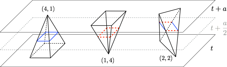
Figure 2: The three fundamental building blocks of CDT in $2+1$ dimensions which interpolate between two consecutive spatial hypersurfaces at integer times $t$ and $t+a$, cf. Fig. 1 in Ref. Ambjorn:2001br . The numbers at the pyramids and the tetrahedron refer to the number of vertices in the quadrangulations at constant integer time $t$ and $t+a$. In between, their intersections with the $t+\frac{a}{2}$-plane are shown, giving rise to an equilateral quadrangulation thereof in terms of blue, red and bi-colored squares. The colorization emphasizes that $2+1$ dimensional information is encoded in a $2d$ setting with colors.

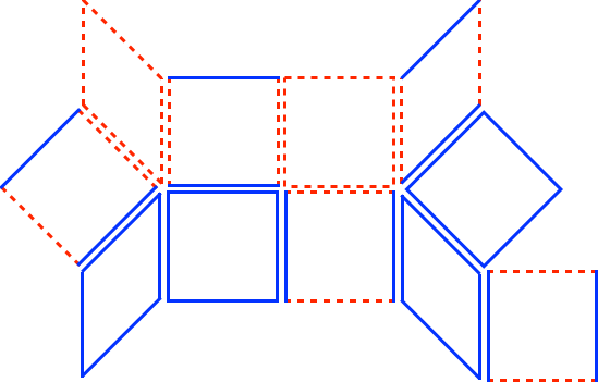
Figure 3: Snapshot of a quadrangulation of the intermediate $t+\frac{a}{2}$-plane, cf. Fig. 2 in Ref. Ambjorn:2001br .

Indeed, the entire information on the CDT partition function can be encoded in the one-step propagator which provides the transition amplitude between the spatial hypersurfaces at $t$ and $t+a$. It is this property that enables a connection to the $ABAB$ matrix model. Indeed, it has been shown in Ambjorn:2001br that the Euclideanized transition amplitude between the triangulation $\Delta$ of the spatial hypersurface $\Sigma_{t}$ and $\Delta(\Sigma_{t+a})$ is given by (cf. Eq. 6 in Ambjorn:2001br )

$$\langle\Delta(\Sigma_{t+a})|\hat{T}|\Delta(\Sigma_{t})\rangle =\langle N_{14}|\hat{T}|N_{41}\rangle$$

$$=\text{e}^{-(\lambda-\kappa)(N_{41}+N_{14})}\sum_{N_{22}=N_{22}^{\text{min}}}^{N_{22}^{\text{max}}}\mathcal{N}_{\text{CDT}}(N_{41},N_{14},N_{22})\text{e}^{-(\frac{1}{2}\lambda+\kappa)N_{22}},$$ (3)

where $\hat{T}$ is the transfer matrix. In the above expression, $N_{41}$ is the number of squares at $t$ and there are $N_{14}$ squares in $t+a$. The sum is over all intermediate quadrangulations, and $\mathcal{N}_{\text{CDT}}(N_{41},N_{14},N_{22})$ denotes the total number of quadrangulations at fixed $N_{22}$. We note that this expression holds for spaces of spherical topology triangulated by a large number of squares. Further, the above expression assumes the discretized Einstein-Hilbert action, such that $\lambda$ and $\kappa$ are related to the bare cosmological constant $\Lambda$ and bare Newton coupling $G_{N}$ as follows

$$\kappa=\frac{a}{4\pi G_{\text{N}}}\left(-\pi+3\arccos{\frac{1}{3}}\right),\leavevmode\nobreak\ \leavevmode\nobreak\ \leavevmode\nobreak\ \lambda=\frac{a^{3}\Lambda}{24\sqrt{2}\pi},$$ (4)

and $a$ is the lattice spacing.

Finally, introducing the dimensionless boundary constant $z_{t}$ understood as a cosmological term for the boundary area, one can set up the discrete Laplace transform of the transfer matrix,

$$\langle z_{t+a}|\hat{T}|z_{t}\rangle=\sum_{N_{41},N_{14}}\text{e}^{-z_{t}N_{41}-z_{t+a}N_{14}}\langle N_{14}|\hat{T}|N_{41}\rangle,$$ (5)

which together with the identifications

$$\bar{\alpha}_{1}=\text{e}^{\kappa-\lambda-z_{t}},\leavevmode\nobreak\ \leavevmode\nobreak\ \leavevmode\nobreak\ \bar{\alpha}_{2}=\text{e}^{\kappa-\lambda-z_{t+a}},\leavevmode\nobreak\ \leavevmode\nobreak\ \leavevmode\nobreak\ \bar{\beta}=\text{e}^{-\frac{1}{2}\lambda+\kappa},$$ (6)

makes the close relation of the free energy of the matrix model,

$$N^{\prime 2}F=-\ln Z[0,0]=\sum_{N_{41},N_{14},N_{22}}\mathcal{N}_{\text{MM}}(N_{41},N_{14},N_{22})\bar{\alpha}_{1}^{N_{41}}\bar{\alpha}_{2}^{N_{14}}\bar{\beta}^{N_{22}},$$ (7)

to the CDT-partition function obvious.

However, the number of configurations generated by the CDT model is smaller than that generated by the matrix model, i.e., $\mathcal{N}_{\text{MM}}>\mathcal{N}_{\text{CDT}}$: The matrix model generically generates disconnected subgraphs via so-called touching interactions (see below). This is most easily seen by switching off the interactions in one sector, $\bar{\alpha}_{2}\rightarrow 0$ and integrating out $B$. The resulting single-matrix model contains multi-trace terms. In the dual triangulation picture, these lead to branched trees of spherical bubbles, see Fig. 4. Clearly, in the generalized situation where $\bar{\alpha}_{2}$ is reinstated, touching interactions will also be present and yield such undesirable quadrangulations. Such pathologies of the local geometry are disallowed by construction in CDT Ambjorn:2012jv .

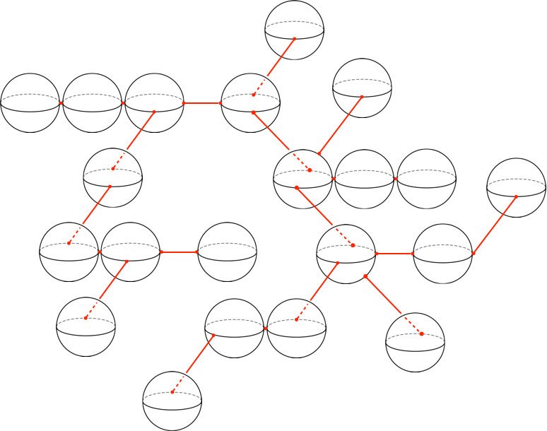
Figure 4: Snapshot of a network of spheres at time $t$ which touch each other at most once at points or are connected by single edges of the quadrangulation caused by so-called touching interactions in the dual matrix model description at $t+\frac{a}{2}$.

Despite these differences, the similarities between the $ABAB$ matrix model and CDTs reinforce the more general notion that causality can be imposed on matrix and tensor models by enlarging the field content of the model and introducing a second matrix/tensor that ultimately enables a distinction of spacelike and timelike edges in the dual triangulation. This motivates us to perform a functional RG analysis of the $ABAB$ matrix model. On the one hand, a comparison to existing results in the literature will enable us to conduct a novel, powerful test of the performance of this technique. On the other hand, this will pave the way for future studies of multi-field models that encode causality in the interaction structure.

3 FRG analysis of the $2$-matrix model with $ABAB$ interaction

3.1 FRG method for matrix models

The FRG is a powerful and versatile tool to implement the Wilsonian renormalization program. In a standard, local field-theoretic setting, given the Euclidean path integral, one introduces a regulator function which suppresses the functional integration of modes below a given momentum cutoff $k$ which correspond to the slow modes in the Wilsonian perspective. By progressively lowering the values of $k$, one carries out the complete integration over all modes. Hence, instead of performing the path integral at once, it is computed in a momentum-shell-wise fashion. The central object in the FRG is the so-called flowing action $\Gamma_{k}$ which interpolates between the classical action $S$ (when $k\to\infty$) and the full effective action $\Gamma$ (when $k\to 0$). It satisfies a flow equation Wetterich:1992yh ; Morris:1993qb which has a simple one-loop structure, making it very efficient for practical calculations, where approximations have to be employed. As the full propagator enters, nonperturbative physics is captured, despite the one-loop structure. At the formal level, the equation is exact and no approximation enters its derivation, rendering it formally equivalent to the path integral. For a recent review of the FRG in a broad range of contexts from condensed matter to quantum gravity, see Dupuis:2020fhh .

The Wilsonian picture as described above relies on a background structure which provides a notion of momentum scales. Such a momentum scale is used as a coarse-graining parameter. In the case of matrix models for quantum gravity, there is no such background. Indeed, these models can be thought of as pre-geometric, with a smooth spacetime and notions of distance emerging in the continuum limit. Yet, as introduced in Ref. Brezin:1992yc , a notion of renormalization group can naturally be defined if the number of entries of the matrices is taken as the coarse-graining parameter, see also Ref. Bonnet:1998ei for an extension of this idea to the case of two-matrix models. Hence, integrating out “fast modes" corresponds to integrating out the outermost rows and columns. In Ref. Eichhorn:2013isa , this idea was translated into an exact flow equation for matrix models, paving the way for similar developments in group field theories Benedetti:2014qsa and tensor models Eichhorn:2017xhy . More recent developments can be found in Refs. Eichhorn:2018ylk ; Eichhorn:2019hsa ; Lahoche:2019ocf ; perezsanchez2020multimatrix , see also Eichhorn:2018phj for a review. For a matrix model defined by the partition function,

$$Z[J]=\int\mathrm{d}M\,\mathrm{e}^{-S[M]+\mathrm{Tr}\left(JM\right)}\,,$$ (8)

where $M$ denotes a Hermitian $N^{\prime}\times N^{\prime}$ matrix, $J$ an external ($N^{\prime}\times N^{\prime}$-matrix) source and $S[M]$ the classical action of the model, one adds a regulator function $\Delta S_{N}$ to the Boltzmann factor of the partition function and obtains the scale-dependent partition function $Z_{N}[J]$,

$$Z_{N}[J]=\int\mathrm{d}M\,\mathrm{e}^{-S[M]-\Delta S_{N}+\mathrm{Tr}\left(JM\right)}\,.$$ (9)

We demand that the regulator $\Delta S_{N}$ has the structure of

$$\Delta S_{N}=\frac{1}{2}\sum_{a,b,c,d}M_{ab}R^{ab,cd}_{N}(a,b)M_{cd}\,,$$ (10)

with $R_{N}$ being independent of the random matrix $M$. It is required to satisfy the following three properties:

$$\lim_{a/N\to 0,\leavevmode\nobreak\ b/N\to 0}R_{N}(a,b)_{ab,cd}>0,$$ (11)

$$\lim_{N/a\to 0,\leavevmode\nobreak\ N/b\to 0}R_{N}(a,b)_{ab,cd}=0,$$ (12)

$$\lim_{N\to N^{\prime}\to\infty}R_{N}(a,b)_{ab,cd}\to\infty,$$ (13)

which suppress the matrix entries in the block $a,b=1,...,N$ and facilitate that the “UV” matrix entries with $a,b>N$ are integrated out Eichhorn:2013isa . It is then a formal manipulation to show that the flowing action $\Gamma_{N}[M]$ defined by

$$\Gamma_{N}[M]=\mathrm{sup}_{J}\left(\mathrm{Tr}(JM)-\mathrm{ln}\leavevmode\nobreak\ Z_{N}\right)-\Delta S_{N}\,,$$ (14)

satisfies

$$\partial_{t}\Gamma_{N}=\frac{1}{2}\mathrm{Tr}\left[\left(\frac{\delta^{2}\Gamma_{N}}{\delta M\delta M}+R_{N}\right)^{-1}\partial_{t}R_{N}\right]\,.$$ (15)

Indices were suppressed for simplicity. The $\mathrm{Tr}$ represents a sum over the indices and $\partial_{t}\equiv N\partial_{N}$. Such a derivative should actually be a finite difference at finite $N$. However, we are interested in the large-$N$ limit, justifying the explicit use of the derivative. The flowing action $\Gamma_{N}$ contains all terms compatible with the symmetries of the model. Thus, it can be expanded as

$$\Gamma_{N}[M]=\sum_{I}\bar{g}_{I}\,\mathcal{O}^{I}[M]\,,$$ (16)

with $\mathcal{O}[M]$ denoting all the operators satisfying a given symmetry and $\bar{g}_{I}$ standing for “dimensionful” couplings. By expanding the right-hand side of Eq. (15) in terms of the same basis $\left\{\mathcal{O}^{I}\right\}$, it is possible to project out the flow of each coupling $\bar{g}_{I}$, i.e., to compute the beta functions of the theory. In standard local field-theoretic settings, one is interested in the dimensionless version of the couplings and their flow as these contain the information on (quantum) scale invariant points. In the present case, there is no local notion of scale; nevertheless “dimensionless” couplings can be defined that absorb factors of $N$. Specificially, the coupling $\bar{g}_{I}$ is related to its dimensionless counterpart $g_{I}$ by the relation $\bar{g}_{I}=N^{[d_{I}]}g_{I}$, where $[d_{I}]$ denotes the canonical scaling dimension of $\bar{g}_{I}$. Since the renormalization group parameter $N$ is dimensionless, the assignment of canonical dimensions to couplings does not follow from simple dimensional analysis. Actually, as discussed in Eichhorn:2014xaa ; Eichhorn:2017xhy ; Eichhorn:2018ylk , the scaling with $N$ is fixed by demanding that, at large-$N$, the system of beta functions is non-trivial and autonomous, i.e., the flow does not depend explicitly on $N$. One can follow similar arguments in the framework of Dyson-Schwinger equations, see, e.g., Pascalie:2018nrs as well as the Polchinski equation Krajewski:2015clk . The beta functions of the dimensionless couplings are thus

$$\partial_{t}g_{I}=-[d_{I}]g_{I}+N^{-[d_{I}]}\partial_{t}\bar{g}_{I}\,.$$ (17)

The function $\partial_{t}\bar{g}_{I}$ is read off from the flow equation (15) by a suitable projection onto the basis defined by Eq. (16).

In this work, we are interested in multi-matrix models. As in standard field theory with multiple fields, the flow equation can easily be derived in this setting. For concreteness, we consider a model with two interacting Hermitian matrices $A$ and $B$ (but the argument extends to a generic set of matrices) with the following partition function,

$$Z[J_{A},J_{B}]=\int\mathrm{d}A\mathrm{d}B\,\mathrm{e}^{-S[A,B]+\mathrm{Tr}\left(J_{A}A\right)+\mathrm{Tr}\left(J_{B}B\right)}\,,$$ (18)

with $J_{A}$ and $J_{B}$ being the sources associated, respectively, to $A$ and $B$ and $S[A,B]$ is the classical action of the model. The regulator $\Delta S_{N}$ is introduced as

$$\Delta S_{N}=\frac{1}{2}\sum_{I,J}\sum_{a,b,c,d}\Phi^{I}_{ab}R^{ab,cd}_{N,IJ}(a,b)\Phi^{J}_{cd}\,,$$ (19)

where $\Phi^{I}\equiv\left\{A,B\right\}$ and $R^{ab,cd}_{N,IJ}(a,b)$ satisfies the properties (11), (12) and (13) transferred to the multi-matrix case. Thence, the flow equation is derived in full analogy to the single-matrix model, leading to

$$\partial_{t}\Gamma_{N}=\frac{1}{2}\mathrm{Tr}\left[\sum_{I,J}\left(\frac{\delta^{2}\Gamma_{N}}{\delta\Phi\delta\Phi}+R_{N}\right)^{-1}_{IJ}\partial_{t}R_{N,JI}\right]\,,$$ (20)

where $\mathrm{Tr}$ represents a sum over matrix indices. Equation (20) easily extends to a generic number of matrices. In the next subsections, we will explicitly apply it to the case of the two-matrix model related to CDT in $2+1$ dimensions, the details of which we specified above.

As it is crucial for the developments that follow, we emphasize an important property of the flow equation: While the path integral Eq. (18) requires the specification of a classical action $S$, the flow equation is independent of the classical action. Instead, it provides a local vector field in the space of all couplings, indicating how the dynamics changes under a finite RG step. A classical action can be specified as an initial condition to integrate this flow and obtain the effective action. On the other hand, the flow equation can also be used to search for special points in the space of couplings, which correspond to fixed points of the RG flow. Such fixed points then give rise to a particular proposal for a classical (or microscopic) action as the starting point of the flow.

3.2 General setup of the flow equations

To obtain the set of beta functions of the couplings, one has to project the flowing action onto the couplings of the corresponding operators. In practice, this is achieved by means of a series expansion of the rhs of Eq. (20) in terms of powers of $A$ and $B$, the $\mathcal{P}^{-1}\mathcal{F}$ expansion. To this end, one rewrites the denominator of the flow equation as

$$\Gamma_{N}^{(2)}+R_{N}=\mathcal{P}_{N}+\mathcal{F}_{N}$$ (21)

with the fluctuation matrix $\mathcal{F}_{N}$ and inverse propagator defined by

$$\mathcal{P}_{N}=\left(\Gamma_{N}^{(2)}+R_{N}\right)\Big{|}_{A=B=0},\qquad\mathrm{\rm and}\qquad\mathcal{F}_{N}=\Gamma_{N}^{(2)}-\left(\Gamma_{N}^{(2)}\Big{|}_{A=B=0}\right)\,.$$ (22)

The right-hand side of the flow equation is then expanded as

$$\partial_{t}\Gamma_{N} =\frac{1}{2}\mathrm{STr}\left[\left(\Gamma_{N}^{(2)}+R_{N}\right)^{-1}\partial_{t}R_{N}\right]$$

$$=\frac{1}{2}\mathrm{STr}\left[\left(\sum_{n=0}^{+\infty}(-1)^{n}\left(\mathcal{P}_{N}^{-1}\mathcal{F}_{N}\right)^{n}\right)\mathcal{P}_{N}^{-1}\,\partial_{t}R_{N}\right],$$ (23)

wherein $\mathrm{STr}$ denotes a sum over the available matrices and the indices thereof. In the next step, we split the Hermitian matrices $A$ and $B$ into symmetric and anti-symmetric parts

$$A_{ab}=A_{1ab}+iA_{2ab},\qquad\mathrm{and}\qquad B_{ab}=B_{1ab}+iB_{2ab}\,,$$ (24)

where $A_{1ab}=A_{1ba}$, $A_{2ab}=-A_{2ba}$, $B_{1ab}=B_{1ba}$ and $B_{2ab}=-B_{2ba}$ hold. With this parameterization, we compute the variations for the Hessian. After doing that, the next step typically is to choose a particular field configuration which facilitates the projection of the right-hand side of the flow equation onto the corresponding beta function of interest. For the purposes of this work, it suffices to take $A_{2ab}=B_{2ab}=0$. The Hessian then has the following structure,

$$\left(\Gamma_{N}^{(2)}\right)_{ab,cd}=\begin{pmatrix}\Gamma_{N,A_{1}A_{1}}&0&\Gamma_{N,A_{1}B_{1}}&0\\ 0&\Gamma_{N,A_{2}A_{2}}&0&\Gamma_{N,A_{2}B_{2}}\\ \Gamma_{N,B_{1}A_{1}}&0&\Gamma_{N,B_{1}B_{1}}&0\\ 0&\Gamma_{N,B_{2}A_{2}}&0&\Gamma_{N,B_{2}B_{2}}\end{pmatrix}_{ab,cd}.$$ (25)

In the very last step, after having computed the beta functions which also map combinatorial differences between operators of the same power in $A$ and $B$, we project the remaining field configurations onto $A_{1ab}=a_{1}\delta_{ab}$ and $B_{1ab}=b_{1}\delta_{ab}$, see Sec. 3.3.

The regulator is chosen in a diagonal form

$$\left(R_{N}\right)_{ab,cd}=\begin{pmatrix}R_{N,A_{1}A_{1}}&0&0&0\\ 0&R_{N,A_{2}A_{2}}&0&0\\ 0&0&R_{N,B_{1}B_{1}}&0\\ 0&0&0&R_{N,B_{2}B_{2}}\end{pmatrix}_{ab,cd}$$ (26)

with

$$R_{N,A_{1}A_{1}/A_{2}A_{2}}(a,b)_{ab,cd} = R_{N,AA}(a,b)\left(\delta_{ac}\delta_{bd}\pm\delta_{ad}\delta_{bc}\right)$$ (27)

$${\equiv} \frac{Z_{A}}{2}f_{N}(a,b)\left(\delta_{ac}\delta_{bd}\pm\delta_{ad}\delta_{bc}\right),$$

and

$$R_{N,B_{1}B_{1}/B_{2}B_{2}}(a,b)_{ab,cd} = R_{N,BB}(a,b)\left(\delta_{ac}\delta_{bd}\pm\delta_{ad}\delta_{bc}\right)$$ (28)

$${\equiv} \frac{Z_{B}}{2}f_{N}(a,b)\left(\delta_{ac}\delta_{bd}\pm\delta_{ad}\delta_{bc}\right).$$

Therein, $Z_{A},Z_{B}$ are wave-function renormalization factors and the details of the cut-off procedure are captured by the function

$$f_{N}(a,b)=\left(\frac{2N}{a+b}-1\right)\theta\left(1-\frac{a+b}{2N}\right),$$ (29)

so that the regulator is closely modelled after Litim’s cutoff Litim:2001up . With these expressions, the computation of the inverse propagator $\mathcal{P}_{N}$, Eq. (22), is straightforward. A relevant detail repeatedly used in the $\mathcal{P}^{-1}\mathcal{F}$ expansion for concrete calculations is then given by the approximation

$$\sum_{a}\sum_{b}\left(\frac{1}{1+f_{N}(a,b)}\right)^{n} \partial_{t}R_{N,AA/BB}(a,b)$$

$$\sim N^{2}\frac{4\left(2+n-\eta_{A/B}\right)}{2+3n+n^{2}}\left(1+\mathcal{O}\left(1/N\right)\right),$$ (30)

valid at leading order in $1/N$. In this expression, we introduce the anomalous dimensions as $\eta_{A/B}=-\partial_{t}\ln Z_{A/B}$.

Finally, as discussed in Refs. Eichhorn:2013isa ; Eichhorn:2018phj and Sec. 3.1, the couplings in matrix and tensor models have an inherent dimensionality in spite of having no natural notion of momentum- scale. It dictates their behavior with respect to rescalings in $N$. In our model, one has the following rescalings for the dimensionful couplings

$$\bar{\alpha}_{1/2}=\frac{\alpha_{1/2}Z_{A/B}^{2}}{N},$$ (31)

and

$$\bar{\beta}=\frac{\beta Z_{A}Z_{B}}{N}\,,$$ (32)

where $\alpha_{1/2}$ and $\beta$ are “dimensionless” couplings. This assignment of scaling dimensionality is chosen in such a way as to facilitate a $1/N$-expansion of the beta functions where the leading coefficient is $\mathcal{O}(N^{0})$. Because of this choice a sensible continuum limit exists.

Equipped with this we are ready to calculate the beta functions from the flow equation.

3.3 Beta functions and fixed points for the $ABAB$ matrix model

In this work we base our analysis on the simplest possible truncation of the flowing action adapted from the action used in Eq. (2), i.e.,

$$\Gamma_{N}[A,B]=\frac{Z_{A}}{2}\mathrm{Tr}\left(AA\right)+\frac{Z_{B}}{2}\mathrm{Tr}\left(BB\right)-\frac{\bar{\alpha}_{1}}{4}\mathrm{Tr}\left(AAAA\right)-\frac{\bar{\alpha}_{2}}{4}\mathrm{Tr}\left(BBBB\right)-\frac{\bar{\beta}}{2}\mathrm{Tr}\left(ABAB\right).$$ (33)

Compared to the analysis of the single-matrix model Eichhorn:2013isa ; Eichhorn:2014xaa , we stick to the sign conventions of Refs. Kazakov:1998qw ; ZinnJustin:2003kq in which the interaction terms carry a negative sign. There is another single-trace interaction compatible with the symmetries of the model which is $\mathrm{Tr}(ABBA)$. However, the beta function of the coupling associated to this interaction is proportional to itself in this simple truncation. Hence, such a coupling can be consistently set to zero and we do not include it here.

From Eq. (33), one can extract the fluctuation matrix $\mathcal{F}_{N}$ which is the remaining ingredient we need in order to compute the $\mathcal{P}^{-1}\mathcal{F}$ expansion. Its non-vanishing entries are given by:

$$\left(\mathcal{F}_{A_{1}A_{1}}\right)_{ab,cd} = -\frac{\bar{\beta}}{2}\left(B_{1ad}B_{1bc}+B_{1ac}B_{1bd}\right)-\frac{\bar{\alpha}_{1}}{2}\bigl{(}A_{1ad}A_{1bc}+A_{1ac}A_{1bd}+A_{1bn}A_{1dn}\delta_{ac}$$ (34)

$$+A_{1bn}A_{1cn}\delta_{ad}+A_{1an}A_{1dn}\delta_{bc}+A_{1an}A_{1cn}\delta_{bd}\bigr{)},$$

$$\left(\mathcal{F}_{A_{1}B_{1}}\right)_{ab,cd} = -\frac{\bar{\beta}}{2}\left(A_{1dn}B_{1bn}\delta_{ac}+A_{1cn}B_{1bn}\delta_{ad}+A_{1dn}B_{1an}\delta_{bc}+A_{1cn}B_{1an}\delta_{bd}\right),$$ (35)

$$\left(\mathcal{F}_{A_{2}A_{2}}\right)_{ab,cd} = \frac{\bar{\beta}}{2}\left(B_{1ad}B_{1bc}-B_{1ac}B_{1bd}\right)+\frac{\bar{\alpha}_{1}}{2}\bigl{(}A_{1ad}A_{1bc}-A_{1ac}A_{1bd}-A_{1bn}A_{1dn}\delta_{ac}$$ (36)

$$+A_{1bn}A_{1cn}\delta_{ad}+A_{1an}A_{1dn}\delta_{bc}-A_{1an}A_{1cn}\delta_{bd}\bigr{)},$$

$$\left(\mathcal{F}_{A_{2}B_{2}}\right)_{ab,cd} = \frac{\bar{\beta}}{2}\left(-A_{1dn}B_{1bn}\delta_{ac}+A_{1cn}B_{1bn}\delta_{ad}+A_{1dn}B_{1an}\delta_{bc}-A_{1cn}B_{1an}\delta_{bd}\right),$$ (37)

$$\left(\mathcal{F}_{B_{1}B_{1}}\right)_{ab,cd} = -\frac{\bar{\beta}}{2}\left(A_{1ad}A_{1bc}+A_{1ac}A_{1bd}\right)-\frac{\bar{\alpha}_{2}}{2}\bigl{(}B_{1ad}B_{1bc}+B_{1ac}B_{1bd}+B_{1bn}B_{1dn}\delta_{ac}$$ (38)

$$+B_{1bn}B_{1cn}\delta_{ad}+B_{1an}B_{1dn}\delta_{bc}+B_{1an}B_{1cn}\delta_{bd}\bigr{)},$$

$$\left(\mathcal{F}_{B_{2}B_{2}}\right)_{ab,cd} = \frac{\bar{\beta}}{2}\left(A_{1ad}A_{1bc}-A_{1ac}A_{1bd}\right)+\frac{\bar{\alpha}_{2}}{2}\bigl{(}B_{1ad}B_{1bc}-B_{1ac}B_{1bd}-B_{1bn}B_{1dn}\delta_{ac}$$ (39)

$$+B_{1bn}B_{1cn}\delta_{ad}+B_{1an}B_{1dn}\delta_{bc}-B_{1an}B_{1cn}\delta_{bd}\bigr{)}.$$

In the following, we present the computations relevant to obtain the set of beta functions from the flow equation. First, we briefly summarize our line of action: Given the simple truncation, we only need to compute the $\mathcal{P}^{-1}\mathcal{F}$ expansion up to order $2$. At $0$th order one obtains a field-independent constant which can be absorbed in the normalization of the path integral and is thus of no interest hereafter. From the $1$st- order- contributions, we compute the expressions for the anomalous dimensions $\eta_{A}$ and $\eta_{B}$. Then, at $2$nd order we yield the beta functions for the couplings.

Starting off with the $1$st order of the expansion, we have

$$\partial_{t}\Gamma_{N}\Big{|}_{\mathrm{Tr}(A^{2}),\mathrm{Tr}(B^{2})} =-\frac{1}{2}\mathrm{STr}\left[\left(\partial_{t}R_{N}\right)\left(\mathcal{P}_{N}^{-1}\right)\left(\mathcal{F}_{N}\right)\left(\mathcal{P}_{N}^{-1}\right)\right]$$

$$=\sum_{a,b}\Biggl{[}\frac{1}{Z_{A}^{2}}\frac{\partial_{t}R_{N,AA}(a,b)}{(1+f_{N}(a,b))^{2}}\left(\bar{\beta}B_{1aa}B_{1bb}+\bar{\alpha}_{1}A_{1aa}A_{1bb}+2\bar{\alpha}_{1}A_{1bn}A_{1bn}\right)$$

$$+\frac{1}{Z_{B}^{2}}\frac{\partial_{t}R_{N,BB}(a,b)}{(1+f_{N}(a,b))^{2}}\left(\bar{\beta}A_{1aa}A_{1bb}+\bar{\alpha}_{2}B_{1aa}B_{1bb}+2\bar{\alpha}_{2}B_{1bn}B_{1bn}\right)\Biggr{]}.$$ (40)

In the next step we focus only on single-trace contributions and thus discard any occurring double-trace terms (which have the structure $\mathrm{Tr}(\ldots)\mathrm{Tr}(\ldots)$). Then, as discussed in Sec. 3.2, the second part of the projection is applied, namely inserting $A_{1ab}=a_{1}\delta_{ab}$ and $B_{1ab}=b_{1}\delta_{ab}$ and carrying out the summations. At large $N$, this leads to

$$\left(N\partial_{N}\frac{Z_{A}}{2}\right)(Na_{1}^{2})+\left(N\partial_{N}\frac{Z_{B}}{2}\right)(Nb_{1}^{2})$$

$$=\frac{1}{Z_{A}^{2}Z_{B}^{2}}\left[Z_{B}^{2}Z_{A}\bar{\alpha}_{1}a_{1}^{2}N^{2}\frac{(4-\eta_{A})}{3}+Z_{A}^{2}Z_{B}\bar{\alpha}_{2}b_{1}^{2}N^{2}\frac{(4-\eta_{B})}{3}\right]$$

$$=Z_{A}a_{1}^{2}N\alpha_{1}\frac{(4-\eta_{A})}{3}+Z_{B}a_{2}^{2}N\alpha_{2}\frac{(4-\eta_{B})}{3}.$$ (41)

In the last step we used the rescaling of the dimensionful couplings $\bar{\alpha}_{1/2}$, as given in Eq. (31). By comparison with the left-hand side, we extract the anomalous dimensions

$$\eta_{A/B}=\frac{8\alpha_{1/2}}{-3+2\alpha_{1/2}}\,,$$ (42)

which results from the solution of an algebraic equation.

At $2$nd order of the expansion, we obtain

$$\partial_{t}\Gamma_{N}\Big{|}_{\mathrm{Tr}(A^{4}),\mathrm{Tr}(B^{4}),\mathrm{Tr}((AB)^{2})}$$

$$=\frac{1}{2}\mathrm{STr}\left[\left(\partial_{t}R_{N}\right)\left(\mathcal{P}_{N}^{-1}\right)\left(\mathcal{F}_{N}\right)\left(\mathcal{P}_{N}^{-1}\right)\left(\mathcal{F}_{N}\right)\left(\mathcal{P}_{N}^{-1}\right)\right]$$

$$=\frac{1}{2Z_{A}^{3}Z_{B}^{3}}\sum_{a,b}\Biggl{[}\partial_{t}R_{N,AA}(a,b)\left\{\bar{\alpha}_{1}^{2}Z_{B}^{3}S_{1}+\bar{\alpha}_{1}\bar{\beta}Z_{B}^{3}S_{2}+\bar{\beta}^{2}Z_{A}Z_{B}^{2}S_{3}+\bar{\beta}^{2}Z_{B}^{3}S_{4}\right\}$$

$$\qquad+\partial_{t}R_{N,BB}(a,b)\bigl{\{}\bar{\alpha}_{2}^{2}Z_{A}^{3}S_{1}(A\leftrightarrow B)+\bar{\alpha}_{2}\bar{\beta}Z_{A}^{3}S_{2}(A\leftrightarrow B)$$

$$\qquad+\bar{\beta}^{2}Z_{B}Z_{A}^{2}S_{3}(A\leftrightarrow B)+\bar{\beta}^{2}Z_{A}^{3}S_{4}(A\leftrightarrow B)\bigr{\}}\Biggr{]}\,,$$ (43)

where $S_{1}$ to $S_{4}$ are given by

$$S_{1} =8\sum_{h}\frac{A_{1aa}A_{1bn}A_{1hn}A_{1hb}}{(1+f_{N}(a,b))^{2}(1+f_{N}(a,h))}+6\sum_{g,h}\frac{A_{1ah}A_{1ha}A_{1bg}A_{1gb}}{(1+f_{N}(a,b))^{2}(1+f_{N}(g,h))}$$

$$\qquad+4\sum_{g}\frac{A_{1an}A_{1gn}A_{1gm}A_{1ma}}{(1+f_{N}(a,b))^{2}(1+f_{N}(g,b))},$$

$$S_{2} =8\sum_{h}\frac{B_{1aa}B_{1hb}B_{1bn}A_{1hn}}{(1+f_{N}(a,b))^{2}(1+f_{N}(a,h))}+4\sum_{g,h}\frac{A_{1ha}B_{1ha}A_{1gb}B_{1gb}}{(1+f_{N}(a,b))^{2}(1+f_{N}(g,h))},$$

$$S_{3} =4\frac{A_{1bn}B_{1bn}A_{1am}B_{1am}}{(1+f_{N}(a,b))^{3}}+4\sum_{h}\frac{A_{1hn}A_{1bm}B_{1bn}B_{1hm}}{(1+f_{N}(a,b))^{2}(1+f_{N}(a,h))},$$

$$S_{4} =2\sum_{g,h}\frac{B_{1ah}B_{1ah}B_{1bg}B_{1bg}}{(1+f_{N}(a,b))^{2}(1+f_{N}(g,h))}.$$ (44)

Again focusing on the single-trace terms only and setting $A_{1ab}=a_{1}\delta_{ab}$ and $B_{1ab}=b_{1}\delta_{ab}$, at large $N$ one finds

$$-\left(N\partial_{N}\frac{\bar{\alpha}_{1}}{4}\right)(Na_{1}^{4})-\left(N\partial_{N}\frac{\bar{\alpha}_{2}}{4}\right)(Nb_{1}^{4})-\left(N\partial_{N}\frac{\bar{\alpha}_{2}}{2}\right)(Na_{1}b_{1}a_{1}b_{1})$$

$$=\frac{1}{2Z_{A}^{3}Z_{B}^{3}}\Big{[}\frac{Z_{A}}{10}(5-\eta_{A})N^{2}\left(\bar{\alpha}_{1}^{2}Z_{B}^{3}4a_{1}^{4}+\bar{\beta}^{2}Z_{A}Z_{B}^{2}4(a_{1}b_{1}a_{1}b_{1})\right)$$

$$\qquad+\frac{Z_{B}}{10}(5-\eta_{B})N^{2}\left(\bar{\alpha}_{2}^{2}Z_{A}^{3}4b_{1}^{4}+\bar{\beta}^{2}Z_{B}Z_{A}^{2}4(a_{1}b_{1}a_{1}b_{1})\right)\Big{]}$$

$$=\frac{Z_{A}^{2}}{5}(5-\eta_{A})\alpha_{1}^{2}a_{1}^{4}+\frac{Z_{A}Z_{B}}{5}(5-\eta_{A})\beta^{2}(a_{1}b_{1}a_{1}b_{2})$$

$$\qquad+\frac{Z_{B}^{2}}{5}(5-\eta_{B})\alpha_{2}^{2}b_{1}^{4}+\frac{Z_{A}Z_{B}}{5}(5-\eta_{B})\beta^{2}(a_{1}b_{1}a_{1}b_{2}).$$ (45)

In the last step we used the rescaling of the dimensionful couplings $\bar{\alpha}_{1},\bar{\alpha}_{2}$ and $\bar{\beta}$, see Eqs. (31) and (32).

We therefore obtain the following beta functions,

$$\beta_{\alpha_{1}} = \left(2\eta_{A}+1\right)\alpha_{1}-\frac{4}{5}\left(5-\eta_{A}\right)\alpha_{1}^{2},$$ (46)

$$\beta_{\alpha_{2}} = \left(2\eta_{B}+1\right)\alpha_{2}-\frac{4}{5}\left(5-\eta_{B}\right)\alpha_{2}^{2},$$ (47)

$$\beta_{\beta} = \left(\eta_{A}+\eta_{B}+1\right)\beta-\frac{2}{5}\left((5-\eta_{A})+(5-\eta_{B})\right)\beta^{2}.$$ (48)

All three beta functions reflect the exchange symmetry $A\leftrightarrow B$. The same symmetry determines the fixed-point structure: A fixed point must either be symmetric under the exchange $\alpha_{1}\leftrightarrow\alpha_{2}$, or come with a counterpart such that the pair of fixed points can be mapped into each other under this exchange. Furthermore, for $\alpha_{1}=\alpha_{2}=\beta$ the system of beta functions is governed by a single equation, reflecting the fact that the model then exhibits a hidden $\text{U}(1)$ symmetry which is otherwise broken zinnjustin1999matrix ; Kostov:1988fy ; Gaudin:1989vx ; Kostov:1992pn ; Eynard:1992cn ; Eynard:1995nv .
Comparing with previous work, we find agreement with the beta function for the single-matrix quartic coupling reported in Eichhorn:2013isa , as expected (note the difference in sign of the quartic term in the truncation).

As a side remark, we mention that when extending the single-trace truncation used here by the next higher-order term, no contribution of type $\mathrm{Tr}\left((AB)^{3}\right)$ is included in the effective action since it would violate the $\mathbb{Z}_{2}$-symmetry of the model. Enlargening by $\mathrm{Tr}\left(A^{6}\right)$ and $\mathrm{Tr}\left(B^{6}\right)$, only the beta functions for $\alpha_{1}$ and $\alpha_{2}$ receive further contributions in agreement with the single-matrix model limit Eichhorn:2013isa .

3.3.1 Fixed-point structure in the symmetric limit

The system analyzed above lends itself to an enhancement of the symmetry to an $A\leftrightarrow B$ exchange symmetry, which entails a smaller theory space since it requires setting $\alpha_{1}=\alpha_{2}\equiv\alpha$, as well as $\eta_{A}=\eta_{B}$. In addition, when also $\alpha=\beta$ holds, the symmetry of the system is enhanced even further, since the model then displays a $\text{U}(1)$ invariance where the matrices $A$ and $B$ behave as a vector under $\text{U}(1)$ transformations. In these symmetry-enhanced cases we obtain the fixed-point structure in Tab. 1, where we use the convention that the critical exponents $\theta_{i}$ are the eigenvalues of the stability matrix, multiplied by an additional negative sign, i.e.,

$$\theta_{i}=-{\rm eig}\left(\frac{\partial\beta_{g_{a}}}{\partial g_{b}}\right)\Big{|}_{\vec{g}=\vec{g}_{\ast}}.$$ (49)

Herein, $\vec{g}$ denotes the vector of all couplings.

Fixed point	type of FP	$\alpha_{\ast}$	$\beta_{\ast}$	$\theta_{1}$	$\theta_{2}$	$\eta$
A	GFP	0	0	-1	-1	0
B	NGFP (SP)	0	0.25	-1	1	0
D	NGFP (SP)	0.10	0	1.07	-0.43	-0.29
C	NGFP	0.10	0.10	1.07	0.43	-0.29

Table 1: Fixed-point values of the couplings and respective critical exponents in the symmetric limit where $\alpha_{1}=\alpha_{2}\equiv\alpha$ holds. By SP (saddle point) we denote fixed points with one relevant direction, which can act as either IR or UV fixed points of the flow.

For the $\text{U}(1)$ symmetric fixed point C, the first critical exponent, $\theta_{1}=1.07$, is also recovered within the $\text{U}(1)$ symmetric theory space, where only a single quartic interaction exists. The second critical exponent, $\theta_{2}=0.43$, encodes the relevance of $\text{U}(1)$-symmetry-breaking perturbations. Accordingly, we conclude that the enhancement of the symmetry in the IR requires tuning, as the fixed point is not IR attractive from outside the $\text{U}(1)$ symmetric theory space.

At $\alpha=1.5$, we observe a singularity of the flow arising from the non-polynomial structure for the anomalous dimension, cf. Eq. (42) beyond which we have discarded any further zeros of the beta functions. These are characterized by anomalous dimensions beyond the regulator bound $\eta_{\rm max}=1$, which is required for a well-defined regulator, see Meibohm:2015twa ; Eichhorn:2018ylk for more details. Further, they exhibit very large critical exponents $\mathcal{O}(10)$, and therefore fail the a-posteriori-check of the self-consistency of our truncation. The latter is based on the assumption of near-canonical scaling, and therefore requires deviations of the critical exponents from the canonical dimensions to be $\mathcal{O}(1)$. The fixed-point candidates are illustrated in Fig. 5. The critical exponents for these are compatible with our assumption of near-canonical scaling. Further, the anomalous dimension $\eta$ is relatively small. Accordingly, we only find changes of the fixed-point properties at the percent level when we compare to the perturbative approximation, where the $\eta$s arising from loop factors are neglected.

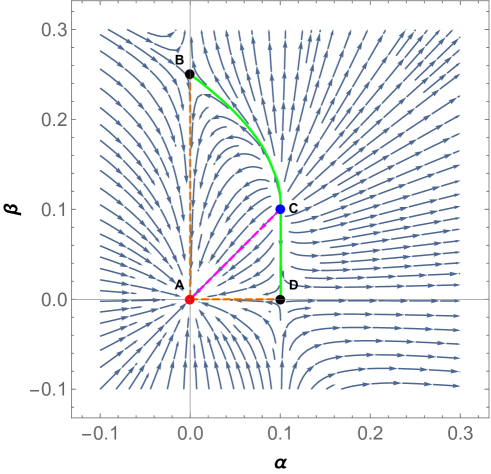
Figure 5: Phase diagram of the $ABAB$ matrix model with $\alpha_{1}=\alpha_{2}=\alpha$ where $4$ fixed points are shown. The black dots ($B,D$) denote saddle points, the red dot ($A$) corresponds to the GFP while the blue dot ($C$) marks the NGFP of interest. For the dashed pink line one has $\alpha=\beta$. Arrows point towards the IR, i.e., small $N$.

3.3.2 Fixed-point structure in the asymmetric case

The more general theory space for the $ABAB$ matrix model does not require the exchange symmetry between $A$ and $B$ to hold at each point during the flow. Accordingly, there can even be fixed points outside the symmetry-enhanced theory space in which $\alpha_{1}=\alpha_{2}$. Such fixed points appear in pairs which are mapped into each other under the mapping $A\leftrightarrow B$. Further, the symmetry-enhanced fixed points from Tab. 1 are also necessarily fixed points of the more general flow. Within the larger theory space, they can be IR attractive or repulsive, i.e., symmetry enhancement can occur as a natural consequence of the flow. In Tab. 2, we list fixed-point candidates and their properties. We highlight the symmetry-enhanced fixed points from Tab. 1 in italics; the additional critical exponent which indicates whether the symmetry-enhancement is an automatic consequence of the flow (which requires $\theta<0$) is indicated in bold.

Fixed point	type of FP	$\alpha_{1\,\ast}$	$\alpha_{2\,\ast}$	$\beta_{\ast}$	$\theta_{1}$	$\theta_{2}$	$\theta_{3}$	$\eta_{A}$	$\eta_{B}$
A	GFP	0	0	0	-1	-1	$\mathbf{-1}$	0	0
D	NGFP (SP)	0	0	0.25	1	-1	-1	0	0
E	NGFP (SP)	0	0.10	0.17	1.07	0.71	-1	0	-0.29
F	NGFP (SP)	0	0.10	0	1.07	-0.71	-1	0	-0.29
C	NGFP (SP)	0.10	0	0.17	1.07	0.71	-1	-0.29	0
B	NGFP (SP)	0.10	0	0	1.07	-0.71	-1	-0.29	0
H	NGFP	0.10	0.10	0.10	1.07	$\mathbf{1.07}$	0.43	-0.29	-0.29
G	NGFP (SP)	0.10	0.10	0	1.07	$\mathbf{1.07}$	-0.43	-0.29	-0.29

Table 2: Fixed-point values of the couplings and respective critical exponents and anomalous dimensions in the case of the asymmetric model where in general $\alpha_{1}\neq\alpha_{2}\neq\beta$ holds. Fixed points which exist in the symmetry-enhanced theory space with $\alpha_{1}=\alpha_{2}$ are indicated in italics, cf. Tab. 1. The additional critical exponent that such fixed points have in the larger theory space are indicated in bold.

As expected, fixed points with $\alpha_{1}\neq\alpha_{2}$ come in pairs which map into each other under $\alpha_{1}\leftrightarrow\alpha_{2}$, cf. third and fifth as well as fourth and sixth line of Tab. 2. It is interesting to observe that at these fixed points, one of the two sectors features no self-interactions, and can therefore be integrated out exactly in the path integral.

An inspection of Tab. 2 highlights that symmetry-enhancement requires fine-tuning, as the additional critical exponent that characterizes the flow of the symmetry-enhanced fixed points in the larger theory space is positive for both cases. Accordingly, the surface $\alpha_{1}=\alpha_{2}$ is likely to be an IR repulsive surface, since both fixed points inside it are. Given that these two fixed points differ by one in the number of their relevant directions, there is a separatrix linking the two, providing a complete trajectory within the symmetry-enhanced fixed point that links a nontrivial universality class in the UV to a nontrivial universality class in the IR. In addition, for $\alpha_{1}=\alpha_{2}=\beta$ the symmetry of the system is further enhanced. The corresponding surface is strongly IR repulsive since the fixed point inside it has three relevant directions. Thus any quartic perturbation away from this symmetry enhancement grows under the RG flow. The fixed points and separatrices which serve to divide the space of microscopic couplings into distinct phases, are shown in Fig. 6.

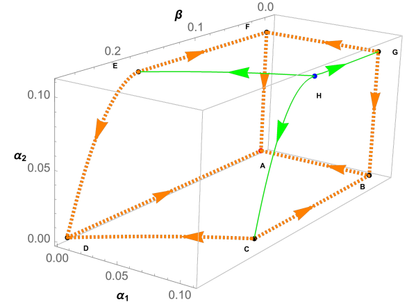
Figure 6: Phase diagram of the $ABAB$ matrix model with $\alpha_{1}\neq\alpha_{2}$ where $8$ fixed points are shown. The black dots ($B,C,D,E,F,G$) denote saddle points, the red dot ($A$) corresponds to the GFP while the blue dot ($H$) marks the NGFP of interest. Arrows point towards the IR, i.e., small $N$.

As expected, we recover $\theta=1.07$ for the fixed point with $\alpha_{1\,\ast}=0=\beta_{\ast}$ (and $\alpha_{2\,\ast}=0=\beta_{\ast}$, respectively). Both of those correspond to the interacting fixed point in the single Hermitian matrix model. In the single-trace approximation, the critical exponent converges to $\theta=1$ from above. As discovered in Eichhorn:2018phj , an alternative prescription for the critical exponents, in which $\eta=\rm const$ is implemented, improves this result to $\theta\rightarrow 0.91$, whereas the exact result, corresponding to the double-scaling limit, is $\theta=0.8$. In the present paper, we work with a simple truncation and do not aim at accuracy in the scaling spectrum, therefore we only provide the critical exponents evaluated according to Eq. (49).

4 Review of the phase diagram of the $ABAB$ matrix model

The two-matrix model with $ABAB$ interaction has been exactly solved in the large $N$ limit Kazakov:1998qw ; ZinnJustin:2003kq using the character expansion method DiFrancesco:1992cn ; Kazakov:1995ae ; Kazakov:1995gm ; Kazakov:1996zm ; Kostov:1997bn . Its phase diagram has been analyzed there and in particular in relation to CDT in $2+1$ dimensions in Ambjorn:2001br ; Ambjorn:2003sr ; Ambjorn:2003ct . Indeed, our results look strikingly similar to theirs, constituting a strong test of the functional RG technique. In particular, we emphasize that we obtain our phase diagrams in the simplest possible truncation of the flowing action. Thus the qualitative agreement is a very promising sign for the performance of the method.
Regarding quantitative results, we can compare, e.g., the critical exponents at the $\alpha_{1}=0=\beta$ fixed point to that of the single-matrix model. As in studies of the single-matrix model in Eichhorn:2013isa , the value for the relevant critical exponent deviates from the exact result corresponding to the string susceptibility $\gamma_{\text{str}}=-\frac{1}{2}$ by about 34 %. At the $\alpha_{1}=0=\alpha_{2}$ fixed point the relevant critical exponent differs by about 17 % from the exact result $\gamma_{\text{str}}=\frac{1}{3}$ Kazakov:1998qw . For fixed points $C$ and $E$ in Tab. 2 the relevant critical exponent is off by 21 % compared to $\gamma_{\text{str}}=-\frac{1}{3}$ Kazakov:1986hu ; ZinnJustin:2003kq . Finally, at the tri-critical point corresponding to the fixed point $H$ in Tab. 2, our result departs by 7 % from the exact value $\gamma_{\text{str}}=0$ Kazakov:1998qw ; ZinnJustin:1999wt ; Kazakov:1988ch . Therefore, an extended truncation is called for to obtain quantitative results for the various universality classes. Additionally, it is an important open question what the impact of higher-order operators, in particular multi-trace ones, is on the full structure of the phase diagram.

Regarding the interpretation of the various phases, we follow the literature, in particular Ambjorn:2001br ; Kazakov:1998qw . The different phases can be distinguished by exploring the behavior of order parameters. For instance, the scaling behavior of the loop average serves as an order parameter which allows to relate the length $L$ of a loop of $A/B$-type of links to the enclosed area $\mathcal{A}$. To make similar arguments solely using FRG technology, the composite-operator renormalization construction Pawlowski:2005xe ; Igarashi:2009tj developed in the context of the Asymptotic Safety program in Pagani:2016dof ; Becker:2018quq ; Houthoff:2020zqy , would have to be carried over to the application of the FRG in the discrete quantum-gravity context.

For the symmetric model ($\alpha_{1}=\alpha_{2}$) with $ABAB$ interaction term, it is possible to identify two distinct continuum phases. In Ambjorn:2001br ; Kazakov:1998qw , the first phase is identified with the line which connects the points $D$ and $C$ in Fig. 5, which is a separatrix in our RG flow. Indeed, initial conditions for the RG flow along that lines are the only ones that lead to the fixed point $D$ as the IR fixed point. At this fixed point, $\beta=0$, which means that one faces two decoupled single-matrix models. A fixed point at finite quartic coupling with one relevant direction is well-known to encode the double-scaling limit Brezin:1992yc ; Eichhorn:2013isa . Thus, its geometric properties match those of $2d$ continuum Liouville quantum gravity Polyakov:1981rd ; DiFrancesco:1993cyw ; david2016liouville which is a model describing a $c=0$ conformal field theory coupled to $2d$ Euclidean quantum gravity, with Hausdorff dimension $d_{\text{H}}=4$ and the scaling relation $\mathcal{A}\sim L^{2}$ Kazakov:1998qw , where $\mathcal{A}$ is the area of a closed loop and $L$ a characteristic length scale of the loop.

The second phase in the symmetric model ($\alpha_{1}=\alpha_{2}$), is identified in Ambjorn:2001br ; Kazakov:1998qw with the line which connects points $B$ and $C$. In our RG flow, this line again corresponds to a separatrix and is the unique RG trajectory that ends in fixed point $B$. For this phase, the geometric properties are not the same as of the other phase in the symmetric model. In spite of also having $c=0$, the critical behavior is different and one finds the anomalous scaling $\mathcal{A}\sim L^{\frac{4}{3}}$, which is that of a branched polymer Jonsson:1997gk ; Ambjorn:1997jf . These results indicate that touching interactions are abundant in the second phase and lead to a fractal structure of the emergent geometry.

Further, we point out that both phases are separated by a phase transition which is marked by the point $C$ in Fig. 5. As noted in Ambjorn:2001br , it is not clear if and how this point can be given an interpretation in terms of three-dimensional geometry and CDT in particular. However, as stated in ZinnJustin:2003kq ; Kazakov:1998qw ; ZinnJustin:1999wt ; Kostov:1999qx , it can be related to a conformal field theory with central charge $c=1$ (i.e., a free and massless boson) coupled to $2d$ Euclidean gravity.

Finally, fixed point $A$ is the free fixed point and therefore only exhibits trivial scaling behavior.

One obtains a somewhat richer phase structure for the general case $\alpha_{1}\neq\alpha_{2}$, see Sec. 3.3.2. Its geometric properties are discussed in ZinnJustin:2003kq ; Ambjorn:2003ct . As far as the relation to CDT in $2+1$ dimensions is concerned, however, only the critical line for which $\alpha_{1}=\alpha_{2}$ holds (corresponding in Fig. 6 to the line which connects the points $H$ and $G$) is relevant Ambjorn:2003ct . Based on this, it has been suggested Ambjorn:2003ct to identify this phase of the matrix model with that of CDT in dimensions $2+1$ Ambjorn:2000dv ; Ambjorn:2001cv which, as shown by numerical evidence Ambjorn:2000dja , corresponds to extended three-dimensional spacetimes with Hausdorff dimension $d_{\text{H}}=4$ for the spatial slices, in line with the value found for $2d$ Euclidean gravity. Notice, however, that without a more detailed grasp of the transfer matrix and thus of the Hamiltonian operator, it is not possible to more precisely characterize the interactions between the adjacent spatial slices and to understand how it analytically encodes the time evolution and thus the generation of extended three-dimensional geometries, so far only numerically observed by means of Monte-Carlo simulations in CDT Ambjorn:2000dja ; Ambjorn:2012jv .

5 Discussion and outlook

In this article, we have pursued the goal to further develop functional Renormalization Group techniques for matrix and tensor models, with a particular focus on multi-field models that could constitute the key to incorporate causality into the setting. Our leading-order FRG analysis has resulted in a phase diagram in good agreement with the results presented in Kazakov:1998qw , providing a strong test of the functional RG approach to matrix/tensor models and highlighting that already at very low truncation order, key physics aspects are well captured.
To quantitatively characterize the universality classes requires extended truncations, as is obvious, e.g., from a comparison of the 2d Euclidean gravity scaling exponent that we recover in a limiting case which differs from the exact result by 34 %. In the future, a more accurate determination of scaling exponents will allow to bridge the gap to continuum techniques to understand whether the Reuter universality class, in particular in continuum studies with Euclidean signature Litim:2003vp ; Codello:2008vh ; Percacci:2010yk ; Rechenberger:2012pm ; Demmel:2012ub ; Demmel:2013myx ; Demmel:2014sga ; Ohta:2012vb ; Ohta:2013uca or with foliation structure Rechenberger:2012dt ; Biemans:2016rvp ; Biemans:2017zca ; Houthoff:2017oam ; Knorr:2018fdu , can be recovered from the matrix/tensor model setting. At the same time, this would also allow to understand whether another gravitational universality class, that related to the tentative asymptotically free fixed point in Hořava-Lifshitz gravity Horava:2009uw ; Benedetti:2013pya ; Contillo:2013fua ; DOdorico:2014tyh ; DOdorico:2015pil ; Barvinsky:2015kil ; Barvinsky:2017kob ; Barvinsky:2019rwn , can be recovered from the present setting, see Horava:2009if ; Benedetti:2009ge ; Ambjorn:2010hu ; Anderson:2011bj ; Sotiriou:2011mu ; Budd:2011zm ; Ambjorn:2013joa ; Benedetti:2014dra ; Benedetti:2016rwo for studies on the relation between CDT and Hořava-Lifshitz gravity. Indeed one would expect that matrix/tensor models which encode causality should be rich enough to encode various continuum universality classes within their phase diagram. A comparison of the scaling spectrum between continuum and discrete settings can provide a check of this expectation.
Such an improvement in accuracy is expected to arise from an improvement in the truncation. The critical exponents at the fixed points we uncovered here are not incompatible with a truncation principle that follows canonical scaling: As in other matrix and tensor models, an increasing order in powers of $A$ and $B$ as well as number of traces of an interaction decreases the scaling dimension of the associated coupling. For fixed-point candidates for which the deviation of the critical exponent from the canonical scaling dimensions is $\mathcal{O}(1)$, as it is in our case, robust truncations can be constructed by neglecting those interactions which are canonically highly irrelevant ones.
Further, setting up a coarse graining in matrix size $N$ leads to a violation of the $\text{U}(N^{\prime})$ symmetry associated with each of the matrices (where $N^{\prime}$ is a UV cutoff). The resulting Ward-identities have first been solved for matrix models in Eichhorn:2014xaa , where it was used that they become trivial in the tadpole-approximation. The latter is well-suited to characterize the fixed point in matrix models for 2d quantum gravity and might therefore also be viable in the present case of the $ABAB$ matrix model. Beyond the tadpole approximation, the solution of the Ward-identities has been explored in Lahoche:2018ggd ; Lahoche:2018hou ; Lahoche:2019vzy .

Beyond the characterization of the universality class in terms of the critical exponents, an understanding of the emergent geometries is desirable. Within the FRG, the composite-operator formalism Pawlowski:2005xe ; Igarashi:2009tj ; Pagani:2016dof ; Becker:2018quq ; Houthoff:2020zqy appears well-suited to provide access to, e.g., the scaling of geometric quantities. At the purely formal level, the evaluation of the corresponding flow equations for matrix/tensor models is not expected to be more challenging than for the flow equation for the effective action itself. The main challenge therefore lies in the identification of suitable operators, where one would expect geometric information to be encoded in higher-order operators in the tensor/matrix formalism.

The relation of the $ABAB$ matrix model to a causal model of dynamical triangulations is an example to highlight a promising route to impose causality in matrix/tensor models: To take into account the presence of both timelike and spacelike edges in a triangulation, a multi-field approach seems indicated, see for instance Kawabe:2020oiw . The present article as well as the recent application of the FRG to a model of non-commutative spacetime with two fields perezsanchez2020multimatrix highlights that the FRG is well-suited to study such models. The present article lays the ground for extensions to higher-rank models.

Beyond the encoding of causality, multi-field models could also account for the interplay of quantum gravity with matter Brezin:1989db ; Bonzom:2012qx ; Lahoche:2019orv , providing yet another motivation to extend the present study to tensor models in the future.

- (1) P. Di Francesco, P.H. Ginsparg and J. Zinn-Justin, 2-D Gravity and random matrices, Phys. Rept. 254 (1995) 1 [hep-th/9306153].
- (2) R. Gurau, Invitation to Random Tensors, SIGMA 12 (2016) 094 [1609.06439].
- (3) R. Gurau, Random tensors, Oxford University Press (2017).
- (4) V. Rivasseau, The Tensor Track, IV, PoS CORFU2015 (2016) 106 [1604.07860].
- (5) N. Delporte and V. Rivasseau, The Tensor Track V: Holographic Tensors, in Proceedings, 17th Hellenic School and Workshops on Elementary Particle Physics and Gravity (CORFU2017): Corfu, Greece, September 2-28, 2017, 2018 [1804.11101].
- (6) E. Witten, An SYK-Like Model Without Disorder, J. Phys. A 52 (2019) 474002 [1610.09758].
- (7) V. Rosenhaus, An introduction to the SYK model, 1807.03334.
- (8) A. Eichhorn and T. Koslowski, Towards phase transitions between discrete and continuum quantum spacetime from the Renormalization Group, Phys. Rev. D90 (2014) 104039 [1408.4127].
- (9) A. Eichhorn, J. Lumma, A.D. Pereira and A. Sikandar, Universal critical behavior in tensor models for four-dimensional quantum gravity, JHEP 02 (2020) 110 [1912.05314].
- (10) J. Ambjorn, J. Jurkiewicz and R. Loll, Dynamically triangulating Lorentzian quantum gravity, Nucl. Phys. B 610 (2001) 347 [hep-th/0105267].
- (11) J. Ambjorn, A. Goerlich, J. Jurkiewicz and R. Loll, Nonperturbative Quantum Gravity, Phys. Rept. 519 (2012) 127 [1203.3591].
- (12) R. Loll, Quantum Gravity from Causal Dynamical Triangulations: A Review, Class. Quant. Grav. 37 (2020) 013002 [1905.08669].
- (13) A. Eichhorn and T. Koslowski, Continuum limit in matrix models for quantum gravity from the Functional Renormalization Group, Phys. Rev. D88 (2013) 084016 [1309.1690].
- (14) A. Eichhorn and T. Koslowski, Flowing to the continuum in discrete tensor models for quantum gravity, Ann. Inst. H. Poincare Comb. Phys. Interact. 5 (2018) 173 [1701.03029].
- (15) A. Eichhorn, T. Koslowski, J. Lumma and A.D. Pereira, Towards background independent quantum gravity with tensor models, 1811.00814.
- (16) A. Eichhorn, T. Koslowski and A.D. Pereira, Status of background-independent coarse-graining in tensor models for quantum gravity, Universe 5 (2019) 53 [1811.12909].
- (17) V. Lahoche and D. Ousmane Samary, Revisited functional renormalization group approach for random matrices in the large- limit, Phys. Rev. D 101 (2020) 106015 [1909.03327].
- (18) D. Benedetti, J. Ben Geloun and D. Oriti, Functional Renormalisation Group Approach for Tensorial Group Field Theory: a Rank-3 Model, JHEP 03 (2015) 084 [1411.3180].
- (19) D. Benedetti and V. Lahoche, Functional Renormalization Group Approach for Tensorial Group Field Theory: A Rank-6 Model with Closure Constraint, Class. Quant. Grav. 33 (2016) 095003 [1508.06384].
- (20) J. Ben Geloun, R. Martini and D. Oriti, Functional Renormalization Group analysis of a Tensorial Group Field Theory on , EPL 112 (2015) 31001 [1508.01855].
- (21) J. Ben Geloun, R. Martini and D. Oriti, Functional Renormalisation Group analysis of Tensorial Group Field Theories on , Phys. Rev. D 94 (2016) 024017 [1601.08211].
- (22) S. Carrozza and V. Lahoche, Asymptotic safety in three-dimensional SU(2) Group Field Theory: evidence in the local potential approximation, Class. Quant. Grav. 34 (2017) 115004 [1612.02452].
- (23) V. Lahoche and D. Ousmane Samary, Functional renormalization group for the U(1)-T tensorial group field theory with closure constraint, Phys. Rev. D 95 (2017) 045013 [1608.00379].
- (24) V. Lahoche and D. Ousmane Samary, Unitary symmetry constraints on tensorial group field theory renormalization group flow, Class. Quant. Grav. 35 (2018) 195006 [1803.09902].
- (25) V. Lahoche and D. Ousmane Samary, Non-perturbative renormalization group beyond melonic sector: The Effective Vertex Expansion method for group fields theories, Phys. Rev. D 98 (2018) 126010 [1809.00247].
- (26) J. Ben Geloun, T.A. Koslowski, D. Oriti and A.D. Pereira, Functional Renormalization Group analysis of rank 3 tensorial group field theory: The full quartic invariant truncation, Phys. Rev. D97 (2018) 126018 [1805.01619].
- (27) V. Lahoche, D. Ousmane Samary and A.D. Pereira, Renormalization group flow of coupled tensorial group field theories: Towards the Ising model on random lattices, Phys. Rev. D 101 (2020) 064014 [1911.05173].
- (28) E. Baloitcha, V. Lahoche and D. Ousmane Samary, Flowing in discrete gravity models and Ward identities: A review, 2001.02631.
- (29) A.G.A. Pithis and J. Thürigen, (No) phase transition in tensorial group field theory, 2007.08982.
- (30) A.G. Pithis and J. Thürigen, Phase transitions in TGFT: Functional renormalization group in the cyclic-melonic potential approximation and equivalence to O models, 2009.13588.
- (31) T. Krajewski and R. Toriumi, Polchinski’s exact renormalisation group for tensorial theories: Gaussian universality and power counting, J. Phys. A 49 (2016) 385401 [1511.09084].
- (32) T. Krajewski and R. Toriumi, Exact Renormalisation Group Equations and Loop Equations for Tensor Models, SIGMA 12 (2016) 068 [1603.00172].
- (33) J.F. Donoghue, The effective field theory treatment of quantum gravity, AIP Conf. Proc. 1483 (2012) 73 [1209.3511].
- (34) G. ’t Hooft and M.J.G. Veltman, One loop divergencies in the theory of gravitation, Ann. Inst. H. Poincare Phys. Theor. A20 (1974) 69.
- (35) M.H. Goroff and A. Sagnotti, The Ultraviolet Behavior of Einstein Gravity, Nucl. Phys. B266 (1986) 709.
- (36) K.S. Stelle, Renormalization of higher-derivative quantum gravity, Phys. Rev. D 16 (1977) 953.
- (37) J.F. Donoghue and G. Menezes, Arrow of Causality and Quantum Gravity, Phys. Rev. Lett. 123 (2019) 171601 [1908.04170].
- (38) J.F. Donoghue and G. Menezes, Unitarity, stability and loops of unstable ghosts, Phys. Rev. D100 (2019) 105006 [1908.02416].
- (39) P. Horava, Quantum Gravity at a Lifshitz Point, Phys. Rev. D79 (2009) 084008 [0901.3775].
- (40) C.F. Steinwachs, Towards a unitary, renormalizable and ultraviolet-complete quantum theory of gravity, 2004.07842.
- (41) S. Weinberg, Critical phenomena for field theorists, in Understanding the fundamental constituents of matter, pp. 1–52, Springer (1978).
- (42) S. Weinberg, Ultraviolet divergences in quantum theories of gravitation, in General relativity (1979).
- (43) M. Reuter, Nonperturbative evolution equation for quantum gravity, Phys. Rev. D57 (1998) 971 [hep-th/9605030].
- (44) C. Wetterich, Exact evolution equation for the effective potential, Phys. Lett. B 301 (1993) 90 [1710.05815].
- (45) T.R. Morris, The Exact renormalization group and approximate solutions, Int. J. Mod. Phys. A 9 (1994) 2411 [hep-ph/9308265].
- (46) N. Dupuis, L. Canet, A. Eichhorn, W. Metzner, J. Pawlowski, M. Tissier et al., The nonperturbative functional renormalization group and its applications, 2006.04853.
- (47) R. Percacci, An Introduction to Covariant Quantum Gravity and Asymptotic Safety, vol. 3 of 100 Years of General Relativity, World Scientific (2017), 10.1142/10369.
- (48) A. Eichhorn, An asymptotically safe guide to quantum gravity and matter, Front. Astron. Space Sci. 5 (2019) 47 [1810.07615].
- (49) M. Reuter and F. Saueressig, Quantum gravity and the functional renormalization group: The road towards asymptotic safety, Cambridge University Press (2018).
- (50) A.D. Pereira, Quantum spacetime and the renormalization group: Progress and visions, in Progress and Visions in Quantum Theory in View of Gravity: Bridging foundations of physics and mathematics, 4, 2019 [1904.07042].
- (51) M. Reichert, Lecture notes: Functional Renormalisation Group and Asymptotically Safe Quantum Gravity, PoS Modave2019 (2020) 005.
- (52) A. Bonanno, A. Eichhorn, H. Gies, J.M. Pawlowski, R. Percacci, M. Reuter et al., Critical reflections on asymptotically safe gravity, 2004.06810.
- (53) A. Eichhorn, Asymptotically safe gravity, in 57th International School of Subnuclear Physics: In Search for the Unexpected, 2, 2020 [2003.00044].
- (54) J.F. Donoghue, A Critique of the Asymptotic Safety Program, Front. in Phys. 8 (2020) 56 [1911.02967].
- (55) D. Becker and M. Reuter, En route to Background Independence: Broken split-symmetry, and how to restore it with bi-metric average actions, Annals Phys. 350 (2014) 225 [1404.4537].
- (56) K. Falls, Background independent exact renormalisation, 2004.11409.
- (57) M. Demmel and A. Nink, Connections and geodesics in the space of metrics, Phys. Rev. D92 (2015) 104013 [1506.03809].
- (58) M. Visser, How to Wick rotate generic curved spacetime, 1702.05572.
- (59) A. Baldazzi, R. Percacci and V. Skrinjar, Wicked metrics, Class. Quant. Grav. 36 (2019) 105008 [1811.03369].
- (60) A. Baldazzi, R. Percacci and V. Skrinjar, Quantum fields without Wick rotation, Symmetry 11 (2019) 373 [1901.01891].
- (61) E. Manrique, S. Rechenberger and F. Saueressig, Asymptotically Safe Lorentzian Gravity, Phys. Rev. Lett. 106 (2011) 251302 [1102.5012].
- (62) C. Rovelli and L. Smolin, Knot Theory and Quantum Gravity, Phys. Rev. Lett. 61 (1988) 1155.
- (63) C. Rovelli and L. Smolin, Loop Space Representation of Quantum General Relativity, Nucl. Phys. B331 (1990) 80.
- (64) T. Thiemann, Modern Canonical Quantum General Relativity, Cambridge Monographs on Mathematical Physics, Cambridge University Press (2007), 10.1017/CBO9780511755682.
- (65) L. Freidel, Group field theory: An Overview, Int. J. Theor. Phys. 44 (2005) 1769 [hep-th/0505016].
- (66) D. Oriti, The Group field theory approach to quantum gravity, gr-qc/0607032.
- (67) S. Carrozza, Flowing in Group Field Theory Space: a Review, SIGMA 12 (2016) 070 [1603.01902].
- (68) A.G.A. Pithis and M. Sakellariadou, Group field theory condensate cosmology: An appetizer, Universe 5 (2019) 147 [1904.00598].
- (69) J. Ben Geloun and D.O. Samary, 3D Tensor Field Theory: Renormalization and One-loop -functions, Annales Henri Poincare 14 (2013) 1599 [1201.0176].
- (70) J. Ben Geloun, Two and four-loop -functions of rank 4 renormalizable tensor field theories, Class. Quant. Grav. 29 (2012) 235011 [1205.5513].
- (71) S. Carrozza, Group field theory in dimension , Phys. Rev. D 91 (2015) 065023 [1411.5385].
- (72) B. Dittrich, The continuum limit of loop quantum gravity - a framework for solving the theory, in Loop Quantum Gravity: The First 30 Years, A. Ashtekar and J. Pullin, eds., pp. 153–179 (2017), DOI [1409.1450].
- (73) S. Steinhaus, Coarse graining spin foam quantum gravity – a review, Front. in Phys. 8 (2020) 295 [2007.01315].
- (74) C. Delcamp and B. Dittrich, Towards a phase diagram for spin foams, Class. Quant. Grav. 34 (2017) 225006 [1612.04506].
- (75) B. Bahr and S. Steinhaus, Numerical evidence for a phase transition in 4d spin foam quantum gravity, Phys. Rev. Lett. 117 (2016) 141302 [1605.07649].
- (76) S. Steinhaus and J. Thürigen, Emergence of Spacetime in a restricted Spin-foam model, Phys. Rev. D98 (2018) 026013 [1803.10289].
- (77) B. Bahr, G. Rabuffo and S. Steinhaus, Renormalization of symmetry restricted spin foam models with curvature in the asymptotic regime, Phys. Rev. D98 (2018) 106026 [1804.00023].
- (78) R. Loll, Discrete approaches to quantum gravity in four-dimensions, Living Rev. Rel. 1 (1998) 13 [gr-qc/9805049].
- (79) J. Ambjørn, A. Görlich, J. Jurkiewicz and R. Loll, Quantum Gravity via Causal Dynamical Triangulations, in Springer Handbook of Spacetime, A. Ashtekar and V. Petkov, eds., pp. 723–741 (2014), DOI [1302.2173].
- (80) J. Ambjorn and J. Jurkiewicz, Four-dimensional simplicial quantum gravity, Phys. Lett. B278 (1992) 42.
- (81) M.E. Agishtein and A.A. Migdal, Simulations of four-dimensional simplicial quantum gravity, Mod. Phys. Lett. A7 (1992) 1039.
- (82) S. Catterall, J.B. Kogut and R. Renken, Phase structure of four-dimensional simplicial quantum gravity, Phys. Lett. B328 (1994) 277 [hep-lat/9401026].
- (83) S. Bilke, Z. Burda, A. Krzywicki and B. Petersson, Phase transition and topology in 4-d simplicial gravity, Nucl. Phys. Proc. Suppl. 53 (1997) 743 [hep-lat/9608027].
- (84) P. Bialas, Z. Burda, A. Krzywicki and B. Petersson, Focusing on the fixed point of 4-D simplicial gravity, Nucl. Phys. B472 (1996) 293 [hep-lat/9601024].
- (85) B.V. de Bakker, Further evidence that the transition of 4-D dynamical triangulation is first order, Phys. Lett. B389 (1996) 238 [hep-lat/9603024].
- (86) S. Catterall, G. Thorleifsson, J.B. Kogut and R. Renken, Simplicial gravity in dimension greater than two, Nucl. Phys. Proc. Suppl. 53 (1997) 756 [hep-lat/9608042].
- (87) J. Laiho, S. Bassler, D. Coumbe, D. Du and J.T. Neelakanta, Lattice Quantum Gravity and Asymptotic Safety, Phys. Rev. D96 (2017) 064015 [1604.02745].
- (88) J. Ambjorn, L. Glaser, A. Goerlich and J. Jurkiewicz, Euclidian 4d quantum gravity with a non-trivial measure term, JHEP 10 (2013) 100 [1307.2270].
- (89) J. Ambjorn, S. Jain, J. Jurkiewicz and C. Kristjansen, Observing 4-d baby universes in quantum gravity, Phys. Lett. B 305 (1993) 208 [hep-th/9303041].
- (90) J. Ambjorn and J. Jurkiewicz, Scaling in four-dimensional quantum gravity, Nucl. Phys. B451 (1995) 643 [hep-th/9503006].
- (91) R.D. Sorkin, Forks in the road, on the way to quantum gravity, Int. J. Theor. Phys. 36 (1997) 2759 [gr-qc/9706002].
- (92) F. Dowker and S. Surya, Topology change and causal continuity, Phys. Rev. D 58 (1998) 124019 [gr-qc/9711070].
- (93) A. Borde, H. Dowker, R. Garcia, R. Sorkin and S. Surya, Causal continuity in degenerate space-times, Class. Quant. Grav. 16 (1999) 3457 [gr-qc/9901063].
- (94) R.P. Geroch, Topology in general relativity, J. Math. Phys. 8 (1967) 782.
- (95) J. Ambjorn and R. Loll, Nonperturbative Lorentzian quantum gravity, causality and topology change, Nucl. Phys. B536 (1998) 407 [hep-th/9805108].
- (96) J. Ambjorn, S. Jordan, J. Jurkiewicz and R. Loll, A Second-order phase transition in CDT, Phys. Rev. Lett. 107 (2011) 211303 [1108.3932].
- (97) J. Ambjorn, S. Jordan, J. Jurkiewicz and R. Loll, Second- and First-Order Phase Transitions in CDT, Phys. Rev. D 85 (2012) 124044 [1205.1229].
- (98) J. Ambjorn, J. Gizbert-Studnicki, A. Goerlich, J. Jurkiewicz, N. Klitgaard and R. Loll, Characteristics of the new phase in CDT, Eur. Phys. J. C 77 (2017) 152 [1610.05245].
- (99) J. Ambjorn, G. Czelusta, J. Gizbert-Studnicki, A. Goerlich, J. Jurkiewicz and D. Nemeth, The higher-order phase transition in toroidal CDT, JHEP 05 (2020) 030 [2002.01051].
- (100) J. Ambjorn, A. Gorlich, J. Jurkiewicz, A. Kreienbuehl and R. Loll, Renormalization Group Flow in CDT, Class. Quant. Grav. 31 (2014) 165003 [1405.4585].
- (101) L. Lionni and J. Thürigen, Multi-critical behaviour of 4-dimensional tensor models up to order 6, Nucl. Phys. B 941 (2019) 600 [1707.08931].
- (102) V. Rivasseau, Quantum Gravity and Renormalization: The Tensor Track, AIP Conf. Proc. 1444 (2012) 18 [1112.5104].
- (103) D. Benedetti and J. Henson, Imposing causality on a matrix model, Phys. Lett. B678 (2009) 222 [0812.4261].
- (104) J. Ambjorn, J. Jurkiewicz, R. Loll and G. Vernizzi, Lorentzian 3-D gravity with wormholes via matrix models, JHEP 09 (2001) 022 [hep-th/0106082].
- (105) P. Zinn-Justin, The Asymmetric ABAB matrix model, Europhys. Lett. 64 (2003) 737 [hep-th/0308132].
- (106) V.A. Kazakov and P. Zinn-Justin, Two matrix model with ABAB interaction, Nucl. Phys. B546 (1999) 647 [hep-th/9808043].
- (107) P. Zinn-Justin, The Six vertex model on random lattices, Europhys. Lett. 50 (2000) 15 [cond-mat/9909250].
- (108) I.K. Kostov, Exact solution of the six vertex model on a random lattice, Nucl. Phys. B575 (2000) 513 [hep-th/9911023].
- (109) J. Ben Geloun and T.A. Koslowski, Nontrivial UV behavior of rank-4 tensor field models for quantum gravity, 1606.04044.
- (110) A. Sfondrini and T.A. Koslowski, Functional Renormalization of Noncommutative Scalar Field Theory, Int. J. Mod. Phys. A 26 (2011) 4009 [1006.5145].
- (111) C.I. Perez-Sanchez, On multimatrix models motivated by random noncommutative geometry i: the functional renormalization group as a flow in the free algebra, 2020.
- (112) A. Castro and T. Koslowski, Renormalization group approach to the continuum limit of matrix models of quantum gravity with preferred foliation, 2020.
- (113) J. Ambjorn, J. Jurkiewicz and R. Loll, Renormalization of 3-d quantum gravity from matrix models, Phys. Lett. B581 (2004) 255 [hep-th/0307263].
- (114) J. Ambjorn, J. Jurkiewicz, R. Loll and G. Vernizzi, 3-D Lorentzian quantum gravity from the asymmetric ABAB matrix model, Acta Phys. Polon. B34 (2003) 4667 [hep-th/0311072].
- (115) J. Ambjorn, J. Jurkiewicz and R. Loll, Nonperturbative 3-D Lorentzian quantum gravity, Phys. Rev. D64 (2001) 044011 [hep-th/0011276].
- (116) V.A. Kazakov, The Appearance of Matter Fields from Quantum Fluctuations of 2D Gravity, Mod. Phys. Lett. A4 (1989) 2125.
- (117) J. Ambjorn, J. Jurkiewicz and R. Loll, A Nonperturbative Lorentzian path integral for gravity, Phys. Rev. Lett. 85 (2000) 924 [hep-th/0002050].
- (118) E. Brezin and J. Zinn-Justin, Renormalization group approach to matrix models, Phys. Lett. B 288 (1992) 54 [hep-th/9206035].
- (119) G. Bonnet and F. David, Renormalization group for matrix models with branching interactions, Nucl. Phys. B 552 (1999) 511 [hep-th/9811216].
- (120) R. Pascalie, C. Perez-Sanchez, A. Tanasa and R. Wulkenhaar, On the large limit of Schwinger-Dyson equations of a rank-3 tensor field theory, J. Math. Phys. 60 (2019) 7 [1810.09867].
- (121) D.F. Litim, Optimized renormalization group flows, Phys. Rev. D 64 (2001) 105007 [hep-th/0103195].
- (122) P. Zinn-Justin, Some matrix integrals related to knots and links, 1999.
- (123) I.K. Kostov, O() Vector Model on a Planar Random Lattice: Spectrum of Anomalous Dimensions, Mod. Phys. Lett. A4 (1989) 217.
- (124) M. Gaudin and I. Kostov, O(n) MODEL ON A FLUCTUATING PLANAR LATTICE: SOME EXACT RESULTS, Phys. Lett. B220 (1989) 200.
- (125) I.K. Kostov and M. Staudacher, Multicritical phases of the O(n) model on a random lattice, Nucl. Phys. B384 (1992) 459 [hep-th/9203030].
- (126) B. Eynard and J. Zinn-Justin, The O(n) model on a random surface: Critical points and large order behavior, Nucl. Phys. B386 (1992) 558 [hep-th/9204082].
- (127) B. Eynard and C. Kristjansen, Exact solution of the O(n) model on a random lattice, Nucl. Phys. B455 (1995) 577 [hep-th/9506193].
- (128) J. Meibohm, J.M. Pawlowski and M. Reichert, Asymptotic safety of gravity-matter systems, Phys. Rev. D 93 (2016) 084035 [1510.07018].
- (129) P. Di Francesco and C. Itzykson, A Generating function for fatgraphs, Ann. Inst. H. Poincare Phys. Theor. 59 (1993) 117 [hep-th/9212108].
- (130) V.A. Kazakov, M. Staudacher and T. Wynter, Character expansion methods for matrix models of dually weighted graphs, Commun. Math. Phys. 177 (1996) 451 [hep-th/9502132].
- (131) V.A. Kazakov, M. Staudacher and T. Wynter, Almost flat planar diagrams, Commun. Math. Phys. 179 (1996) 235 [hep-th/9506174].
- (132) V.A. Kazakov, M. Staudacher and T. Wynter, Exact solution of discrete two-dimensional R**2 gravity, Nucl. Phys. B471 (1996) 309 [hep-th/9601069].
- (133) I.K. Kostov, M. Staudacher and T. Wynter, Complex matrix models and statistics of branched coverings of 2-D surfaces, Commun. Math. Phys. 191 (1998) 283 [hep-th/9703189].
- (134) V. Kazakov, Ising model on a dynamical planar random lattice: Exact solution, Phys. Lett. A 119 (1986) 140.
- (135) V.A. Kazakov and A.A. Migdal, Recent Progress in the Theory of Noncritical Strings, Nucl. Phys. B311 (1988) 171.
- (136) J.M. Pawlowski, Aspects of the functional renormalisation group, Annals Phys. 322 (2007) 2831 [hep-th/0512261].
- (137) Y. Igarashi, K. Itoh and H. Sonoda, Realization of Symmetry in the ERG Approach to Quantum Field Theory, Prog. Theor. Phys. Suppl. 181 (2010) 1 [0909.0327].
- (138) C. Pagani and M. Reuter, Composite Operators in Asymptotic Safety, Phys. Rev. D95 (2017) 066002 [1611.06522].
- (139) M. Becker and C. Pagani, Geometric operators in the asymptotic safety scenario for quantum gravity, Phys. Rev. D99 (2019) 066002 [1810.11816].
- (140) W. Houthoff, A. Kurov and F. Saueressig, On the scaling of composite operators in asymptotic safety, JHEP 04 (2020) 099 [2002.00256].
- (141) A.M. Polyakov, Quantum Geometry of Bosonic Strings, Phys. Lett. B 103 (1981) 207.
- (142) F. David, A. Kupiainen, R. Rhodes and V. Vargas, Liouville quantum gravity on the riemann sphere, Communications in Mathematical Physics 342 (2016) 869.
- (143) T. Jonsson and J.F. Wheater, The Spectral dimension of the branched polymer phase of two-dimensional quantum gravity, Nucl. Phys. B515 (1998) 549 [hep-lat/9710024].
- (144) J. Ambjorn, D. Boulatov, J.L. Nielsen, J. Rolf and Y. Watabiki, The Spectral dimension of 2-D quantum gravity, JHEP 02 (1998) 010 [hep-th/9801099].
- (145) D.F. Litim, Fixed points of quantum gravity, Phys. Rev. Lett. 92 (2004) 201301 [hep-th/0312114].
- (146) A. Codello, R. Percacci and C. Rahmede, Investigating the Ultraviolet Properties of Gravity with a Wilsonian Renormalization Group Equation, Annals Phys. 324 (2009) 414 [0805.2909].
- (147) R. Percacci and E. Sezgin, One Loop Beta Functions in Topologically Massive Gravity, Class. Quant. Grav. 27 (2010) 155009 [1002.2640].
- (148) S. Rechenberger and F. Saueressig, The phase-diagram of QEG and its spectral dimension, Phys. Rev. D 86 (2012) 024018 [1206.0657].
- (149) M. Demmel, F. Saueressig and O. Zanusso, Fixed-Functionals of three-dimensional Quantum Einstein Gravity, JHEP 11 (2012) 131 [1208.2038].
- (150) M. Demmel, F. Saueressig and O. Zanusso, Fixed Functionals in Asymptotically Safe Gravity, in 13th Marcel Grossmann Meeting on Recent Developments in Theoretical and Experimental General Relativity, Astrophysics, and Relativistic Field Theories, pp. 2227–2229, 2015, DOI [1302.1312].
- (151) M. Demmel, F. Saueressig and O. Zanusso, RG flows of Quantum Einstein Gravity on maximally symmetric spaces, JHEP 06 (2014) 026 [1401.5495].
- (152) N. Ohta, Beta Function and Asymptotic Safety in Three-dimensional Higher Derivative Gravity, Class. Quant. Grav. 29 (2012) 205012 [1205.0476].
- (153) N. Ohta and R. Percacci, Higher Derivative Gravity and Asymptotic Safety in Diverse Dimensions, Class. Quant. Grav. 31 (2014) 015024 [1308.3398].
- (154) S. Rechenberger and F. Saueressig, A functional renormalization group equation for foliated spacetimes, JHEP 03 (2013) 010 [1212.5114].
- (155) J. Biemans, A. Platania and F. Saueressig, Quantum gravity on foliated spacetimes: Asymptotically safe and sound, Phys. Rev. D 95 (2017) 086013 [1609.04813].
- (156) J. Biemans, A. Platania and F. Saueressig, Renormalization group fixed points of foliated gravity-matter systems, JHEP 05 (2017) 093 [1702.06539].
- (157) W. Houthoff, A. Kurov and F. Saueressig, Impact of topology in foliated Quantum Einstein Gravity, Eur. Phys. J. C 77 (2017) 491 [1705.01848].
- (158) B. Knorr, Lorentz symmetry is relevant, Phys. Lett. B 792 (2019) 142 [1810.07971].
- (159) D. Benedetti and F. Guarnieri, One-loop renormalization in a toy model of Hořava-Lifshitz gravity, JHEP 03 (2014) 078 [1311.6253].
- (160) A. Contillo, S. Rechenberger and F. Saueressig, Renormalization group flow of Hořava-Lifshitz gravity at low energies, JHEP 12 (2013) 017 [1309.7273].
- (161) G. D’Odorico, F. Saueressig and M. Schutten, Asymptotic Freedom in Hořava-Lifshitz Gravity, Phys. Rev. Lett. 113 (2014) 171101 [1406.4366].
- (162) G. D’Odorico, J.-W. Goossens and F. Saueressig, Covariant computation of effective actions in Hořava-Lifshitz gravity, JHEP 10 (2015) 126 [1508.00590].
- (163) A.O. Barvinsky, D. Blas, M. Herrero-Valea, S.M. Sibiryakov and C.F. Steinwachs, Renormalization of Hořava gravity, Phys. Rev. D 93 (2016) 064022 [1512.02250].
- (164) A.O. Barvinsky, D. Blas, M. Herrero-Valea, S.M. Sibiryakov and C.F. Steinwachs, Horava Gravity is Asymptotically Free in 2 + 1 Dimensions, Phys. Rev. Lett. 119 (2017) 211301 [1706.06809].
- (165) A.O. Barvinsky, M. Herrero-Valea and S.M. Sibiryakov, Towards the renormalization group flow of Horava gravity in dimensions, Phys. Rev. D100 (2019) 026012 [1905.03798].
- (166) P. Horava, Spectral Dimension of the Universe in Quantum Gravity at a Lifshitz Point, Phys. Rev. Lett. 102 (2009) 161301 [0902.3657].
- (167) D. Benedetti and J. Henson, Spectral geometry as a probe of quantum spacetime, Phys. Rev. D 80 (2009) 124036 [0911.0401].
- (168) J. Ambjorn, A. Gorlich, S. Jordan, J. Jurkiewicz and R. Loll, CDT meets Horava-Lifshitz gravity, Phys. Lett. B 690 (2010) 413 [1002.3298].
- (169) C. Anderson, S.J. Carlip, J.H. Cooperman, P. Horava, R.K. Kommu and P.R. Zulkowski, Quantizing Horava-Lifshitz Gravity via Causal Dynamical Triangulations, Phys. Rev. D 85 (2012) 044027 [1111.6634].
- (170) T.P. Sotiriou, M. Visser and S. Weinfurtner, Spectral dimension as a probe of the ultraviolet continuum regime of causal dynamical triangulations, Phys. Rev. Lett. 107 (2011) 131303 [1105.5646].
- (171) T. Budd, The effective kinetic term in CDT, J. Phys. Conf. Ser. 36 (2012) 012038 [1110.5158].
- (172) J. Ambjørn, L. Glaser, Y. Sato and Y. Watabiki, 2d CDT is 2d Hořava–Lifshitz quantum gravity, Phys. Lett. B 722 (2013) 172 [1302.6359].
- (173) D. Benedetti and J. Henson, Spacetime condensation in (2+1)-dimensional CDT from a Hořava–Lifshitz minisuperspace model, Class. Quant. Grav. 32 (2015) 215007 [1410.0845].
- (174) D. Benedetti and J.P. Ryan, Capturing the phase diagram of (2 + 1)-dimensional CDT using a balls-in-boxes model, Class. Quant. Grav. 34 (2017) 105012 [1612.09533].
- (175) V. Lahoche and D. Ousmane Samary, Ward identity violation for melonic -truncation, Nucl. Phys. B 940 (2019) 190 [1809.06081].
- (176) V. Lahoche and D.O. Samary, Progress in the solving nonperturbative renormalization group for tensorial group field theory, Universe 5 (2019) 86 [1812.00905].
- (177) V. Lahoche and D. Ousmane Samary, Ward-constrained melonic renormalization group flow, Phys. Lett. B 802 (2020) 135173 [1904.05655].
- (178) H. Kawabe, CDT open-closed surface field theory of a 3D tensor-matrix model, 2009.02489.
- (179) E. Brezin, M.R. Douglas, V. Kazakov and S.H. Shenker, The Ising Model Coupled to 2- Gravity: A Nonperturbative Analysis, Phys. Lett. B 237 (1990) 43.
- (180) V. Bonzom and H. Erbin, Coupling of hard dimers to dynamical lattices via random tensors, J. Stat. Mech. 1209 (2012) P09009 [1204.3798].