Bayesian Geodesic Regression on Riemannian Manifolds

Abstract

Geodesic regression has been proposed for fitting the geodesic curve. However, it cannot automatically choose the dimensionality of data. In this paper, we develop a Bayesian geodesic regression model on Riemannian manifolds (BGRM) model. To avoid the overfitting problem, we add a regularization term to control the effectiveness of the model. To automatically select the dimensionality, we develop a prior for the geodesic regression model, which can automatically select the number of relevant dimensions by driving unnecessary tangent vectors to zero. To show the validation of our model, we first apply it in the 3D synthetic sphere and 2D pentagon data. We then demonstrate the effectiveness of our model in reducing the dimensionality and analyzing shape variations of human corpus callosum and mandible data.

1 Introduction

Regression analysis is a predictive modeling technique, which studies the relationship between dependent variables (objectives) and independent variables (predictors). This technique is usually used to predict and analyze the causal relationship between variables. The benefits of regression analysis are numerous, such as: (1) it shows the significant correlation between the independent variable and dependent variable; (2) it shows the influence of multiple independent variables on a dependent variable. Regression analysis also allows us to compare the interactions between variables that measure different scales.

However, linear models are not applicable if the response variable takes the values on the Riemannian manifold. Manifold learning has been applied in many fields, including domain adaption, transformation, tensor and shape measurement [Gopalan et al.(2011)Gopalan, Li, and Chellappa, Gong et al.(2012)Gong, Shi, Sha, and Grauman, Zhang et al.(2019a)Zhang, Xie, and Davison, Rathi et al.(2007)Rathi, Tannenbaum, and Michailovich, Pizer et al.(1999)Pizer, Fritsch, Yushkevich, Johnson, and Chaney, Zhang et al.(2019b)Zhang, Xing, and Zhang]. However, it has difficulty in analyzing the shape variations, which are essentially high-dimensional and nonlinear. Therefore, it is necessary to develop a general regression model and reduce the dimensionality on manifolds.

Several studies have explored the regression issues on the manifolds, which includes unrolling method, regression analysis on the group of diffeomorphisms, nonparametric regression, second order splines, a semiparametric model with multiple covariates, and geodesic regression  [Jupp and Kent(1987), Miller(2004), Davis et al.(2010)Davis, Fletcher, Bullitt, and Joshi, Trouvé and Vialard(2010), Shi et al.(2009)Shi, Styner, Lieberman, Ibrahim, Lin, and Zhu, Fletcher(2011), Zhang(2019)]. However, these methods does not provide a Bayesian framework for the generalization of geodesic regression on manifolds. It is thus necessary to develop such a model to automatically choose the model complexity.

The purpose of this paper is to develop a generalized Bayesian geodesic regression on Riemannian manifolds, termed BGRM model. Our model can estimate the relationship between an independent scalar variable and a dependent manifold-valued random variable. Our work is inspired by the Bayesian principal component analysis (BPCA) model, which is introduced in Euclidean space by Bishop [Bishop(1999)].

We develop a maximum likelihood posterior model for Bayesian geodesic regression on manifolds (BGRM). By introducing a prior to the geodesic regression model, we can automatically select the number of relevant dimensions by driving unnecessary tangent vectors to zero. The main advantage of our Bayesian geodesic regression approach is that the model is fully generative. The unnecessary dimensionality of the subspace will be automatically killed, and the principal models of variation can reconstruct shape deformation of individuals. To show the validation of our model, we first apply it in the 3D synthetic sphere and 2D pentagon data. We then use the human corpus callosum and mandible data to show the predicted shapes using our model. Our results indicate that the BGRM model provides a better description of the data than PCA [Jolliffe(2011)], principal geodesic analysis (PGA) [Fletcher et al.(2004)Fletcher, Lu, Pizer, and Joshi] and probabilistic principal geodesic analysis (PPGA) [Zhang and Fletcher(2013)] estimations. Our model also shows reasonable shape variations with the increasing of age in a much lower-dimensional subspace.

2 Bayesian linear regression on Euclidean space (BLR)

Before formulating Bayesian geodesic regression on Riemannian manifolds, we first review Bayesian linear regression on Euclidean space. Fig. 1(a) shows the scheme of linear regression model. Given the target variable (dependent variable) $y\in\mathbb{R}^{n}$, and independent variable $x\in\mathbb{R}$. The linear regression model is given by:

$$y=\mu+vx+\epsilon,$$ (1)

where $v\in\mathbb{R}^{n}$ is the unobservable slope parameter, $\mu\in\mathbb{R}^{n}$ is the unobservable intercept parameter, and $\epsilon$ is zero mean Gaussian unobservable random variable with the variance $\tau^{-1}$. Thus, we can rewrite Eq. (1) as:

$$p(y|x,\mu,v,\tau)=\mathcal{N}(y|\mu+vx,\tau^{-1}),$$ (2)

where $p(\cdot)$ is the probability, and $\mathcal{N}$ is the normal distribution. Consider a data set of input $X=\{x_{n}\}_{n=1}^{N}$ ($x_{n}\in\mathbb{R}$) with corresponding target value $Y=\{y_{n}\}_{n=1}^{N}$ ($y_{n}\in\mathbb{R}^{n}$ can be treated as column vector with the size of $d\times 1$), and these data points are independently sampled from the normal distribution. Then, the data likelihood is:

$$p(Y|X,\mu,v,\tau)=\prod_{n=1}^{N}\mathcal{N}(y_{n}|\mu+vx_{n},\tau^{-1}).$$ (3)

(a) Linear regression

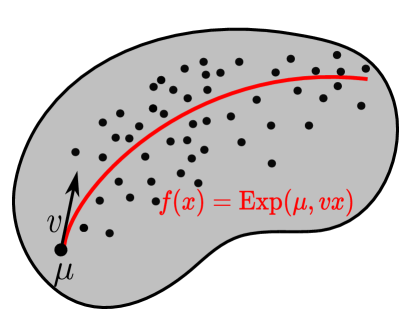
(b) Geodesic regression

Figure 1: (a): Schematic of the linear regression, $\mu$ is one point (the intercept), $v$ is the tangent vector (the slope). The black line is the linear regression line $f(x)=\mu+vx$. (b): Schematic of the geodesic regression on Riemannian manifolds, $\mu$ is a base point on the manifold, $v$ is a point of tangent space. The red line is the geodesic regression line $f(x)=\operatorname{Exp}(\mu,vx)$.

To automatically select the principal component, Bayesian geodesic regression model includes a Gaussian prior over each column of $v$, which is known as an automatic relevance determination (ARD) prior. The $v$ is constrained to a zero-mean isotropic Gaussian distribution with the parameter $\alpha$:

$$p(v|\alpha)=\mathcal{N}(v|0,\alpha^{-1}I).$$ (4)

The logarithm of posterior distribution is given by (see [Bishop(1999)] for details):

$$\text{ln}\ p(v|y)=-\frac{\tau}{2}\sum_{n=1}^{N}\{y_{n}-(\mu+vx_{n})\}^{2}-\frac{\alpha}{2}v^{T}v+\text{const}..$$ (5)

The value of $\alpha$ is iteratively estimated as $\alpha=\frac{N}{v^{T}v}$, if $\alpha_{i}$ (one column of $\alpha$) is large, the corresponding $v_{i}$ will be small and thus enforces sparsity by driving the $v_{i}$ to zero. The sparsity of $v$ has the same effect as removing irrelevant dimensions in the principal subspace.

3 Bayesian geodesic regression on manifolds (BGRM)

3.1 Background: Riemannian Geometry

In this section, we recap three essential concepts (Geodesic, Exponential, and Logarithmic Map) on the Riemannian Geometry (more details are provided by [Zhang and Fletcher(2013), Zhang et al.(2019b)Zhang, Xing, and Zhang, Zhang et al.(2019a)Zhang, Xie, and Davison]).

Geodesic. Let $(M,g)$ be a Riemannian manifold, where $g$ is a Riemannian metric on the manifold $M$. Consider a curve $C(t):[0,1]\rightarrow M$ and let $C^{\prime}(t)=dC/dt$ be its velocity. We call $C$ a geodesic if $C^{\prime}(t)$ is parallel along $C$, that is: $C^{\prime\prime}=\frac{dC^{\prime}}{dt}=\nabla_{C^{\prime}}C^{\prime}=0$, which means the acceleration vector (directional derivative) $C^{\prime\prime}$ is normal to $T_{C(t)}M$ (the tangent space of $M$ at $C(t)$). Note that geodesics are straight lines in Euclidean space ($\mathbb{R}^{n}$).

Exponential Map. For any point $p\in M$ and its tangent vector $v$, let $\mathcal{D}(p)$ be the open subset of $T_{p}M$ defined by: $\mathcal{D}(p)=\{v\in T_{p}M|C(1)\}$, where $C$ is the unique geodesic with initial conditions $C(0)=p$ and $C^{\prime}(0)=v$. The exponential map is the map $\operatorname{Exp}_{p}:\mathcal{D}(p)\rightarrow M$ defined by: $\text{Exp}_{p}(vt_{=1})=C(1)$, which means the exponential map returns the points at $C(1)$ when $t=1$. $\text{Exp}_{p}(vt)$ can also be denoted as: $\text{Exp}(p,vt)$. In Euclidean space, the exponential map is the addition operation $\text{Exp}_{p}(vt)=p+vt$.

Logarithmic Map. Given two points $p$ and $p^{\prime}$ $\in M$, the logarithmic map takes the point pair $(p,p^{\prime})$ and maps them into the tangent space $T_{p}M$, and it is an inverse of the exponential map: $\operatorname{Log}(p,p^{\prime})\rightarrow T_{p}M$. $\operatorname{Log}(p,p^{\prime})$ can also be denoted as: $\operatorname{Log}_{p}p^{\prime}$. Because Log is an inverse of the exponential map, we can also write: $p^{\prime}=\operatorname{Exp}(p,\operatorname{Log}(p,p^{\prime}))$. The Riemannian distance is defined as $d(p,p^{\prime})=\|\text{Log}_{p}(p^{\prime})\|$. In Euclidean space, the logarithmic map is the subtraction operation: $\text{Log}_{p}(p^{\prime})=p^{\prime}-p$.

3.2 Geodesic regression

Geodesic regression has been proposed by Fletcher [Fletcher(2011)], the geodesic regression model is defined as:

$$Y=\operatorname{Exp}(\operatorname{Exp}(\mu,vX),\epsilon),$$ (6)

where $\mu$ is a base point on the manifold, $v$ is a point of tangent space $T_{\mu}M$, $X$ is the independent variable, $Y$ is the observed data and $\epsilon$ is a random variable taking values in the tangent space with the precision $\tau$. Since the exponential map is the addition operation in Euclidean space, the geodesic regression model coincides with Eq. (1) when $M=R^{n}$. Fig. 1(b) shows the scheme of geodesic regression model.

Eq. (7) is the Riemannian normal distribution $\mathcal{N}_{M}(\mu,\tau^{-1})$, with its precision parameter $\tau$. This general distribution can be applied to any Riemannian manifold (see [Zhang and Fletcher(2013)] for details).

$$p(y|\mu,\tau) =\frac{1}{C(\mu,\tau)}\exp\left(-\frac{\tau}{2}d(y,\mu)^{2}\right),\quad\text{where}$$ (7)

$$C(\mu,\tau) =\int_{M}\exp\left(-\frac{\tau}{2}d(y,\mu)^{2}\right)dy.$$

Given a data set of input $X=\{x_{n}\}_{n=1}^{N}$ ($x_{n}\in\mathbb{R}$) with corresponding target value $Y=\{y_{n}\}_{n=1}^{N}$ ($y_{n}\in\mathbb{R}^{n}$ can be treated as column vector with the size of $d\times 1$) on general manifolds. Each target value $y_{n}$ is independent of the Riemannian normal distribution. Therefore, the data likelihood on Riemannian manifolds is defined as:

$$p(Y|X,\mu,v,\tau)=\prod_{n=1}^{N}\mathcal{N}_{M}(y_{n}|\operatorname{Exp}(\mu,vx_{n}),\tau^{-1}).$$ (8)

Taking the logarithm of the Eq. (8), we have

$$\text{ln}\ p(Y|X,\mu,v,\tau) =-N\ \text{ln}\ C-\frac{\tau}{2}\sum_{n=1}^{N}\{\operatorname{Log}(y_{n},\operatorname{Exp}(\mu,vx_{n}))\}^{2}.$$ (9)

3.3 Regularized geodesic regression

The overfitting problem can be caused by a complex model that is trained on a small number of datasets. To avoid the overfitting problem, we add a regularization term in Eq. (9), thus the total energy function (E) is given by:

$$E =\frac{1}{2}\sum_{n=1}^{N}\{\operatorname{Log}(y_{n},\operatorname{Exp}(\mu,vx_{n}))\}^{2}+\frac{\gamma}{2}v^{T}v,$$ (10)

Choosing the optimal dimensionality is significant, we need to find the appropriate number of basis functions to determine a suitable value of the regularization coefficient $\gamma$. Therefore, it is necessary to develop a method which can automatically choose the dimensionality of data.

3.4 Bayesian geodesic regression

To automatically select the principal geodesic from data, we also include a Gaussian prior over each column of $v$. Supposing that $v$ is constrained to a zero-mean isotropic Gaussian distribution, which has a single parameter $\alpha$, so that:

$$p(v|\alpha)=\mathcal{N}(v|0,\alpha^{-1}I).$$ (11)

Since the posterior distribution $p(v|y)$ is proportion to $p(y|x,v,\tau)\times p(v|\alpha)$, the logarithm of posterior distribution is equivalent to take the logarithm of $p(y|x,v,\tau)\times p(v|\alpha)$. Then the log of the data likelihood can be computed as:

$$\mathbb{E}=\text{ln}p(v|y)=-N\ \text{ln}\ C-\frac{\tau}{2}\sum_{n=1}^{N}\{\operatorname{Log}(y_{n},\operatorname{Exp}(\mu,vx_{n}))\}^{2}-\frac{\alpha}{2}v^{T}v+\text{const.}.$$ (12)

Maximization of this posterior distribution with respect to $v$ is equivalent to the minimization of the sum-of-squares error function with the addition of a quadratic regularization term, corresponding to Eq. (10) with $\gamma=\alpha/\tau$.

Similar to the BLR model, the value of $\alpha$ is iteratively estimated as $\alpha=\frac{N}{v^{T}v}$, and then enforces sparsity by driving the corresponding component $v_{i}$ to zero. More specifically, if $\alpha_{i}$ is large, $v_{i}$ will be effectively removed. This arises naturally because the larger $\alpha_{i}$ is, the lower probability of $v_{i}$ will be. Therefore, we can automatically select the dimensionality of $v$, and it has the same effect as removing irrelevant dimensions in the principal subspace. Fig. 2 is the graphical representation of BGRM model.

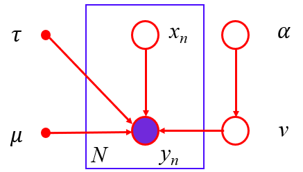
Figure 2: Probabilistic graphical representation of BGRM model. In the blue box, it has $N$ data points, for each independent observation $y_{n}$, it is together with the corresponding independent variable $x_{n}$, and it is associated with $\tau,\mu$ and $v$. Here, $v$ is controlled by the hyperparameter $\alpha$.

3.4.1 Gradient terms

We use gradient descent to maximize the posterior distribution in Eq. (LABEL:lnmre), and update the parameters $\mu,v$ and $\tau$. However, the computation of the gradient term requires us compute the derivative of $\operatorname{Exp}(vx_{n},\mu)$, which can be separated into a derivation with respect to the initial point $\mu$, and respect to the initial velocity $v$ (please refer to [Fletcher(2011)] for the details of derivations).

Now we are able to take the gradient of Eq. (LABEL:lnmre) with respect to different parameters: $\mu,v$ and $\tau$ and get the following gradient terms:

Gradient for $\mu$: the gradient of $\mu$ is

$$\nabla_{\mu}(\mathbb{E})=-\sum_{n=1}^{N}\tau d_{\mu}\text{Exp}(\mu,vx_{n})^{\dagger}\text{Log}(y_{n},\text{Exp}(\mu,vx_{n})),$$ (13)

where $\dagger$ represents adjoint operation, for any $u$ and $w$

$$\langle d_{\mu}\operatorname{Exp}(\mu,vx_{n})u,w\rangle=\langle u,d_{\mu}\operatorname{Exp}(\mu,vx_{n})^{\dagger}w\rangle.$$

Gradient for $v$: the gradient of $v$ can be computed as

$$\nabla_{v}(\mathbb{E}) =-\sum_{n=1}^{N}\tau x_{n}d_{v}\text{Exp}(\mu,vx_{n})^{\dagger}\text{Log}(y_{n},\text{Exp}(\mu,vx_{n}))-\alpha v.$$ (14)

Gradient for $\tau$ : the gradient of $\tau$ is computed as

$$\nabla_{\tau}(\mathbb{E}_{\mathcal{L}}) =\sum_{n=1}^{N}\frac{1}{C(\tau)}A_{n-1}\int_{0}^{R}\frac{r^{2}}{2}\text{Exp}(-\frac{\tau}{2}r^{2})\prod_{k=2}^{n}k_{k}^{-1/2}\times$$ (15)

$$f_{k}(\sqrt{k_{k}}r)dr-\frac{1}{2}\{\operatorname{Log}(y_{n},\operatorname{Exp}(\mu,vx_{n}))\}^{2}dr,$$

where $A_{n-1}$ is the surface area of $n-1$ hypershpere. $r$ is radius, $k_{k}$ is the sectional curvature. $R=\text{min}_{v}{R(v)}$, and $R(v)$ is the maximum distance of $\text{Exp}(\mu,rv)$, $v$ is a point of unit sphere $S^{n-1}\subset T_{\mu}M$. However, this formula only validates for simple connected symmetric spaces, other spaces should be changed according to the different definitions of the probability density function (PDF) in Eq. (7) (please see [Zhang and Fletcher(2013)] for details).

4 Evaluation

4.1 Data

Sphere. To validate our model on the spherical manifold, we simulate a random sample of $293$ data points (3D) on a unit sphere with known parameters (ground truth) in Table 1. The points are randomly sampled given the $\mu$, $v$, and the precision $\tau$ (please refer to [Fletcher and Zhang(2016)] for generating points on a sphere). The ground truth $\mu$ is generated from random uniform points on the sphere, and $v$ is generated from a random Gaussian matrix.

Table 1: Parameters comparison between ground truth and the estimation of BGRM, PGA and PCA models ($[\cdot]^{T}$ is the transpose of a matrix).

	$\mu$	$v$	$\tau$
Ground truth	$[0.7704,0.4155,0.4836]^{T}$	$\left[\begin{matrix}0.0755&-0.2771&-0.2784\\ -0.0002&0.0007&0.0100\\ \end{matrix}\right]^{T}$	100
BGRM	$[0.8728,0.2916,0.3913]^{T}$	$\left[\begin{matrix}0.0739&-0.2577&-0.2239\\ \end{matrix}\right]^{T}$	98.3399
PPGA [Zhang and Fletcher(2013)]	$[0.8674,0.2735,0.4157]^{T}$	$\left[\begin{matrix}0.0773&-0.2849&-0.1873\\ -0.0006&0.0012&0.0098\\ \end{matrix}\right]^{T}$	103.817
PGA [Fletcher et al.(2004)Fletcher, Lu, Pizer, and Joshi]	$[0.8848,0.2850,0.3687]^{T}$	$\left[\begin{matrix}0.0752&-0.1070&-0.0978\\ -0.0076&0.0748&0.0761\\ \end{matrix}\right]^{T}$	N/A
PCA [Jolliffe(2011)]	$[0.8680,0.2797,0.3618]^{T}$	$\left[\begin{matrix}0.0717&-0.1065&-0.0979\\ -0.0083&0.0746&0.0751\\ \end{matrix}\right]^{T}$	N/A

In Table 1, the recovered parameters $\mu,v$, and $\tau$ of our BGRM model are closer to ground truth than three baseline methods (PPGA, PGA and PCA). We can visualize the estimated geodesic in Fig. 3. The blue line is the true geodesic. The red line is the estimated geodesic of BGRM model, and the green line is the estimated geodesic of PPGA model. Although both the PPGA and BGRM model can recover the geodesic, our BGRM model kills the unnecessary dimensionality of $v$. The true $v$ has the size of $3\times 2$, and our BGRM model kills the second column, which is much smaller than the first column. This result demonstrates the ability of our model in automatical dimensionality selection.

To show the correctness of our model, we also compare the estimation results of our model with PCA in the Euclidean space. As shown in Fig. 3, the estimated geodesic of BGRM model is a curve on the sphere, but the estimated geodesic of PCA is a straight line, which is below the sphere. And this leads to the unobserved PCA results on the sphere.

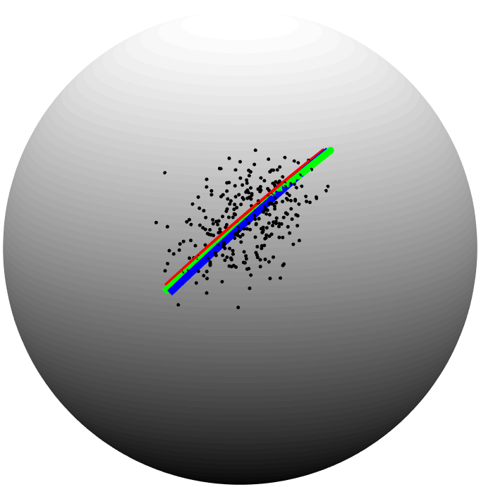
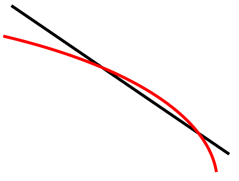
Figure 3: (a): Geodesic regression on sphere using BGRM and PPGA model. The blue line is the ground truth geodesic. The red line is the estimated geodesic of BGRM model. The green line is the estimated geodesic of PPGA model. (b): The comparison of estimated geodesic of BGRM and PCA model. The red line is the estimated geodesic of BGRM in (a). The black line is the estimated geodesic using PCA, which is a straight line (below the sphere) and cannot be visualized in (a).

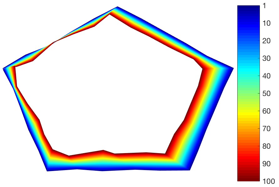
(a) Shape variations of pentagon

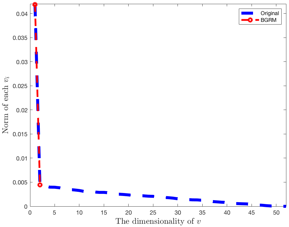
(b) Reduced dimensionality

Figure 4: The shape variations of pentagon and reduced dimensionality using BGRM model. (a): The color from blue to red is the corresponding $x$ of each shape. The shape shrinks with the increasing of $x$. (b): BGRM model automatically selects the first two dimensionalities out of 52 in total.

Pentagon. To evaluate our model in a high dimensional data, we first apply the BGRM model in analyzing shape variations of synthetic pentagon dataset. This synthetic data contains a collection of 50 pentagon shapes with $x$ from 1 to 50. Each pentagon has the $2\times 26$ points. We aim to predict the new pentagon shapes when $x$ is from 51 to 100. The regression result is shown in Fig. 4(a). The pentagon shape shrinks with the increasing of the $x$. This example illustrates our model is applicable in analyzing the shape variations of data. In addition, Fig. 4(b) shows that our BGRM model reduces the dimensionality of pentagon data from $52$ to $2$. The red dash line is the reduced number of the tangent vector ($v$), and the blue dash line is the original number of $v$.

Corpus Callosum Aging. To show the effectiveness of BGRM model in the real shape changes, we use corpus callosum data, which are extracted from the MRI scans of human brains. This data contains a collection of 40 shapes with age from 0 to 80 years. Each corpus callosum shape has the $2\times 65$ points. As shown in Fig. 5, we show the corpus callosum shape changes using the BGRM and BLR model. From Fig. 5(a), there are more changes with the increasing of age in the posterior part of the corpus callosum. This result is significantly better than the regression results in BLR model, in which shapes are almost overlaying with each other due to the shape geometry does not consider in the Euclidean space of BLR model. Also, as shown in Fig. 5(b), our BGRM model reduces the dimensionality of corpus callosum data from $130$ to $31$. Dimensionality is omitted in Fig. 5(c) if it is greater than 45.

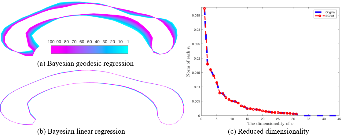
Figure 5: The regression results comparison of BGRM (a) and BLR (b) model using corpus callosum data. The estimated shapes are shown as the sequence from 1 (cyan) to 100 (pink). The color bar indicates the age in years. (c): The reduced dimensionality of BGRM model.

Mandible shape. We also evaluate our BGRM model in estimating the shape variations of human mandible growths. The mandible data are extracted from a collection of CT scans of human mandibles. It contains $77$ subjects and the age is from $0$ to $19$ years. We sample $2\times 400$ points on the boundaries. Fig. 6(a) shows the estimated mandible shape variations using BGRM model, there are more variations in the head part of mandible shape. When the age is between 14 and 20 years, the mandible is dramatically increased, which coincides with the results in [Sharma et al.(2014)Sharma, Arora, and Valiathan]. As shown in Fig. 6(b), our BGRM model reduces the dimensionality of mandible data from $800$ to $76$. Dimensionality is omitted in Fig. 6(b) if it is greater than 100.

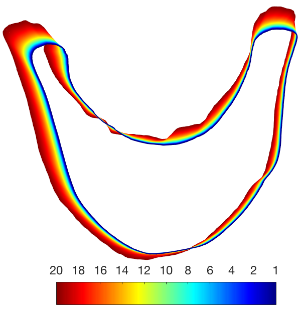
(a) Estimated mandible shapes

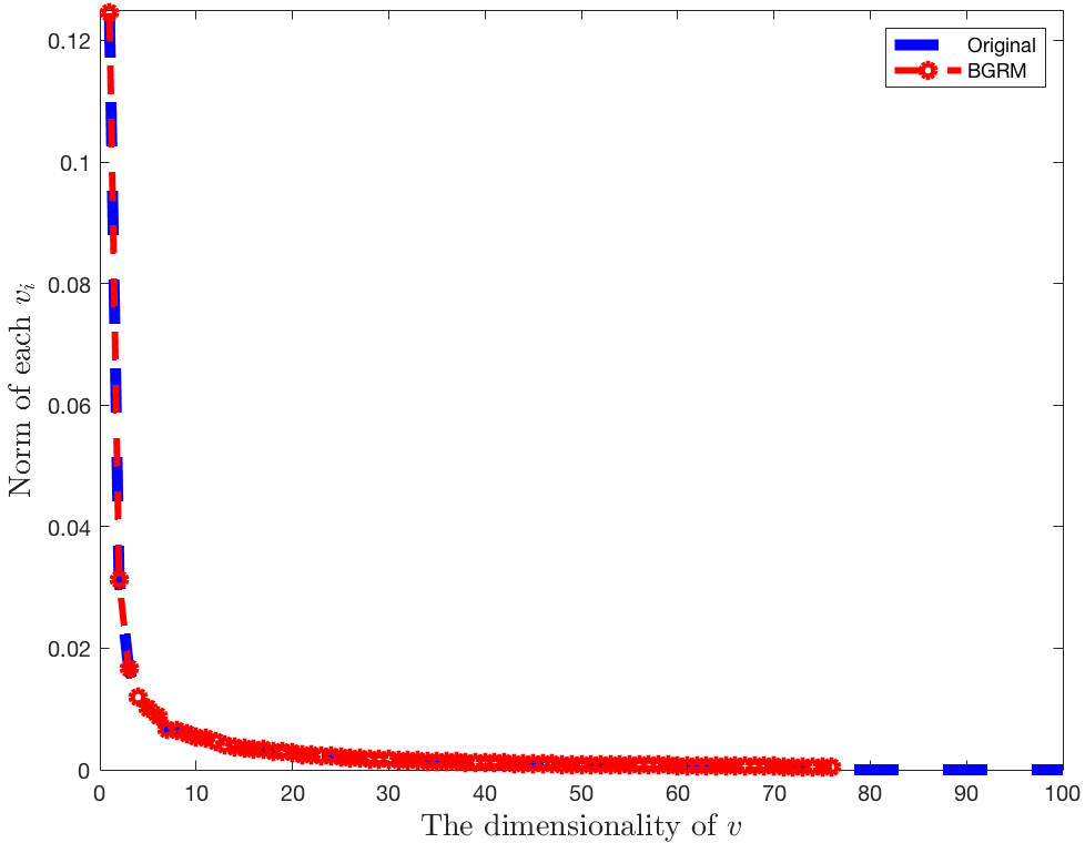
(b) Reduced dimensionality comparison

Figure 6: (a): The estimated human mandible shape using BGRM; (b): The comparison of original dimensionality and reduced dimensionality of BGRM model.

Table 2: $R^{2}$ statistic of predicting shapes

Datasets	Pentagon	Corpus callosum	Mandible
Linear regression	0.0135	0.0194	0.0518
Geodesic regression [Fletcher(2011)]	0.0223	0.0234	0.0873
ShapeNet [Zhang and Davison(2019)]	0.3911	0.3854	0.1738
BGRM	0.4318	0.4279	0.2146

4.2 Significance analysis

To show the significance of our model, we report the $R^{2}$ value in Eq. (16), which is between $[0,1]$. The higher the $R^{2}$ value is, the more variations are explained by the model, and the better of model in predicting the shape.

$$R^{2}=1-\frac{\text{Unexplained variation }}{\text{Total variation}}=1-\frac{\sum_{i=1}^{N}(y_{i}-y_{i}^{\prime})^{2}}{\sum_{i=1}^{N}(y_{i}-\bar{y})^{2}},$$ (16)

where $y_{i}^{\prime}$ is the predicted shape, $\bar{y}$ is the mean shape of $Y$ and $N$ is the number of shapes.

Table 2 compares the $R^{2}$ statistic of our BGRM model with linear regression, geodesic regression model and ShapeNet. The $R^{2}$ values of three datasets from our BGRM model are larger than that of other models. The lower value of the geodesic regression model means that shape variability is not well modeled by age since age only describes a small fraction of the shape variation. Other factors (gender, weight, etc.) can also affect shape changes. However, the coefficient of determination ($R^{2}$ values) of our model demonstrates that age is an important factor that affects these shapes. Therefore, our BGRM model is better than state-of-the-art methods and effective in predicting shape variations.

5 Discussion

From the above experiments, we find that the proposed BGRM model is able to predict the shape changes with a higher $R^{2}$ value. Although the $R^{2}$ value of the mandible dataset is not as significant as the other two datasets, which is caused by little variations of the original data, BGRM model still has a higher $R^{2}$ value than three baseline methods. In addition, we also calculate the p-values of three datasets (0.7485, 0.9780, and 0.3478, respectively). These results imply that predicting shapes are similar to true shapes. However, one weakness of our model is that it is sensitive to large changes in shape.

6 Conclusion

In this paper, we develop a Bayesian geodesic regression model on Riemannian manifolds. By introducing a prior to the geodesic regression model, we can automatically select the number of relevant dimensions by driving unnecessary tangent vectors to zero. We use maximum a posterior method to estimate model parameters. Four experimental results indicate that our BGRM model takes the advantages of automatically reducing the dimensionality of the subspace and shows the reasonable shape variations. There are some obvious next steps. More data can be applied in our model. The model can also be extended to develop a Bayesian poly-nomial geodesic regression model on Riemannian manifolds.

References

- [Bishop(1999)] Christopher M Bishop. Bayesian pca. In Advances in neural information processing systems, pages 382–388, 1999.
- [Davis et al.(2010)Davis, Fletcher, Bullitt, and Joshi] Brad C Davis, P Thomas Fletcher, Elizabeth Bullitt, and Sarang Joshi. Population shape regression from random design data. International journal of computer vision, 90(2):255–266, 2010.
- [Fletcher(2011)] P Thomas Fletcher. Geodesic regression on riemannian manifolds. In Proceedings of the Third International Workshop on Mathematical Foundations of Computational Anatomy-Geometrical and Statistical Methods for Modelling Biological Shape Variability, pages 75–86, 2011.
- [Fletcher and Zhang(2016)] P Thomas Fletcher and Miaomiao Zhang. Probabilistic geodesic models for regression and dimensionality reduction on riemannian manifolds. In Riemannian Computing in Computer Vision, pages 101–121. Springer, 2016.
- [Fletcher et al.(2004)Fletcher, Lu, Pizer, and Joshi] P Thomas Fletcher, Conglin Lu, Stephen M Pizer, and Sarang Joshi. Principal geodesic analysis for the study of nonlinear statistics of shape. IEEE transactions on medical imaging, 23(8):995–1005, 2004.
- [Gong et al.(2012)Gong, Shi, Sha, and Grauman] Boqing Gong, Yuan Shi, Fei Sha, and Kristen Grauman. Geodesic flow kernel for unsupervised domain adaptation. In Computer Vision and Pattern Recognition (CVPR), 2012 IEEE Conference on, pages 2066–2073. IEEE, 2012.
- [Gopalan et al.(2011)Gopalan, Li, and Chellappa] Raghuraman Gopalan, Ruonan Li, and Rama Chellappa. Domain adaptation for object recognition: An unsupervised approach. In Computer Vision (ICCV), 2011 IEEE International Conference on, pages 999–1006. IEEE, 2011.
- [Jolliffe(2011)] Ian Jolliffe. Principal component analysis. In International encyclopedia of statistical science, pages 1094–1096. Springer, 2011.
- [Jupp and Kent(1987)] Peter E Jupp and John T Kent. Fitting smooth paths to speherical data. Applied statistics, pages 34–46, 1987.
- [Miller(2004)] Michael I Miller. Computational anatomy: shape, growth, and atrophy comparison via diffeomorphisms. NeuroImage, 23:S19–S33, 2004.
- [Pizer et al.(1999)Pizer, Fritsch, Yushkevich, Johnson, and Chaney] Stephen M Pizer, Daniel S Fritsch, Paul A Yushkevich, Valen E Johnson, and Edward L Chaney. Segmentation, registration, and measurement of shape variation via image object shape. IEEE Transactions on Medical Imaging, 18(10):851–865, 1999.
- [Rathi et al.(2007)Rathi, Tannenbaum, and Michailovich] Yogesh Rathi, Allen Tannenbaum, and Oleg Michailovich. Segmenting images on the tensor manifold. In Computer Vision and Pattern Recognition, 2007. CVPR’07. IEEE Conference on, pages 1–8. IEEE, 2007.
- [Sharma et al.(2014)Sharma, Arora, and Valiathan] Padmaja Sharma, Ankit Arora, and Ashima Valiathan. Age changes of jaws and soft tissue profile. The Scientific World Journal, 2014, 2014.
- [Shi et al.(2009)Shi, Styner, Lieberman, Ibrahim, Lin, and Zhu] Xiaoyan Shi, Martin Styner, Jeffrey Lieberman, Joseph G Ibrahim, Weili Lin, and Hongtu Zhu. Intrinsic regression models for manifold-valued data. In International Conference on Medical Image Computing and Computer-Assisted Intervention, pages 192–199. Springer, 2009.
- [Trouvé and Vialard(2010)] Alain Trouvé and François-Xavier Vialard. A second-order model for time-dependent data interpolation: Splines on shape spaces. In MICCAI STIA Workshop, 2010.
- [Zhang and Fletcher(2013)] Miaomiao Zhang and P Thomas Fletcher. Probabilistic principal geodesic analysis. In Advances in Neural Information Processing Systems, pages 1178–1186, 2013.
- [Zhang(2019)] Youshan Zhang. K-means principal geodesic analysis on riemannian manifolds. In Proceedings of the Future Technologies Conference, pages 578–589. Springer, 2019.
- [Zhang and Davison(2019)] Youshan Zhang and Brian D Davison. Shapenet: Age-focused landmark shape prediction with regressive cnn. In 2019 International Conference on Content-Based Multimedia Indexing (CBMI), pages 1–6. IEEE, 2019.
- [Zhang et al.(2019a)Zhang, Xie, and Davison] Youshan Zhang, Sihong Xie, and Brian D Davison. Transductive learning via improved geodesic sampling. In Proceedings of the 30th British Machine Vision Conference, 2019a.
- [Zhang et al.(2019b)Zhang, Xing, and Zhang] Youshan Zhang, Jiarui Xing, and Miaomiao Zhang. Mixture probabilistic principal geodesic analysis. In Multimodal Brain Image Analysis and Mathematical Foundations of Computational Anatomy, pages 196–208. Springer, 2019b.