CHIMPS2: Survey description and ¹²CO emission in the Galactic Centre

Abstract

The latest generation of Galactic-plane surveys is enhancing our ability to study the effects of galactic environment upon the process of star formation. We present the first data from CO Heterodyne Inner Milky Way Plane Survey 2 (CHIMPS2). CHIMPS2 is a survey that will observe the Inner Galaxy, the Central Molecular Zone (CMZ), and a section of the Outer Galaxy in ¹²CO, ¹³CO, and C¹⁸O $(J\,=\,3\rightarrow 2)$ emission with the Heterodyne Array Receiver Program on the James Clerk Maxwell Telescope (JCMT). The first CHIMPS2 data presented here are a first look towards the CMZ in ¹²CO J = 3$\rightarrow$2 and cover $-3\degr\,\leq\,\ell\,\leq\,5\degr$ and $\mid$b$\mid\,\leq\,0\aas@@fstack{\circ}5$ with angular resolution of 15 arcsec, velocity resolution of 1 km s^-1, and rms $\Delta\,T_{A}^{\ast}=$ 0.58 K at these resolutions. Such high-resolution observations of the CMZ will be a valuable data set for future studies, whilst complementing the existing Galactic Plane surveys, such as SEDIGISM, the Herschel infrared Galactic Plane Survey, and ATLASGAL. In this paper, we discuss the survey plan, the current observations and data, as well as presenting position-position maps of the region. The position-velocity maps detect foreground spiral arms in both absorption and emission.

1 Introduction

The formation of stars from molecular gas is the key process driving the evolution of galaxies from the early Universe to the current day. However, the regulation of the efficiency of this process (the star-formation efficiency; SFE) on both the small scales of individual clouds and the larger scales of entire galaxies, is poorly understood.

In the era of ALMA, single-dish surveys play an essential role for understanding star formation in the context of Galactic environment. Advances in array detectors have enabled large surveys of the Galactic Plane to be completed in a reasonable time, producing large samples of regions for statistical analysis (e.g., Urquhart et al., 2018). By doing this, we can measure the relative impact on the SFE of Galactic-scale processes, e.g., spiral arms, or the pressure and turbulence within individual clouds.

However, untangling star formation on larger and smaller scales is complicated by the different sampling rates on these scales. Studies of extragalactic systems have produced empirical relationships, such as the Kennicutt–Schmidt (K–S) relationship (Kennicutt, 1998), which scales the star-formation rate (SFR) with gas density; and further relationships scaling the SFR with the quantity of dense gas ($n(\mathrm{H}_{\mathrm{2}})\geq 3\,\times 10^{4}$ cm^-3; Gao & Solomon 2004; Lada et al. 2012). These correlations, though, break down on scales of 100–500 pc, a scale where the enclosed sample of molecular clouds is small (Onodera et al., 2010; Schruba et al., 2010; Kruijssen & Longmore, 2014).

These two apparently contradictory results are supported when the clump-formation efficiency (CFE), or dense-gas mass fraction (DGMF) within individual molecular clouds is examined. The distribution of cloud CFEs is lognormal, with values varying by 2–3 orders of magnitude (Eden et al., 2012; Eden et al., 2013); however, the CFE is fairly constant when averaged over kiloparsec scales.

The distributions of the SFEs estimated from the ratio of infrared luminosity to cloud or clump gas mass, are also found to be lognormal (Eden et al., 2015), indicating that the central-limit theorem is at play in both cases, giving a well defined mean value when averaged over a large sample of clouds and a large area of the Galaxy. They also point to the spiral structures of the Milky Way having only a minor influence in enhancing the star formation within them (Moore et al. 2012; Urquhart et al., in preparation), a conclusion also reached in M51 (Schinnerer et al., 2017). The fraction of star-forming Herschel sources as a function of Galactocentric radius in the Milky Way also displays no arm-associated signal (Ragan et al., 2016, 2018). Studies of other Galactic-scale mechanisms, such as shear, have found conflicting evidence for impact on the star formation (Dib et al., 2012; Suwannajak et al., 2014).

Despite these results, there are large-scale variations between Galactic environments that would be expected to have significant influence on the star-formation process. The three major star-formation stages: the conversion of atomic to molecular gas, the conversion of molecular gas to dense star-forming clumps (DGMF and CFE), then the formation of stars (SFE), all show some significant variations related to Galactocentric radius. The molecular-gas mass fraction rapidly decreases from $\sim$ 100 per cent within the inner 1 kpc to a few per cent at $\sim$ 10 kpc (Sofue & Nakanishi, 2016). The DGMF peaks at 3–4 kpc, and drops within the Galactic centre, where the disc may become stable against large-scale gravitational collapse (Kruijssen et al., 2014), whilst the SFE also drops dramatically in the central 0.5 kpc when compared to the dense gas (Longmore et al., 2013; Urquhart et al., 2013). These reductions are within the region swept by the bar where, in external galaxies, the SFR is suppressed for the life of the bar (James & Percival, 2016, 2018). However, when compared to the total gas mass, the SFE is consistent with the K–S relationship (Yusef-Zadeh et al., 2009; Sormani et al., 2020).

The physics of molecular clouds are important in regulating star formation, since triggering and local environment are only thought to cause 14–30 per cent of star formation (Thompson et al., 2012; Kendrew et al., 2012). There is some evidence that the clouds in the Central Molecular Zone (CMZ) exhibit low SFE as they are subject to mainly solenoidal turbulence (Federrath et al., 2016), as opposed to the compressive turbulence found in spiral-arm clouds. Therefore, to examine the internal physics, high-resolution observations of large samples of molecular clouds are required in different transitions and isotopologues such as the ¹³CO/C¹⁸O $(J\,=\,3\rightarrow 2)$ Heterodyne Inner Milky Way Plane Survey (CHIMPS; Rigby et al. 2016), the CO High-Resolution Survey (COHRS; Dempsey et al. 2013), the FOREST Unbiased Galactic-plane Imaging survey with the Nobeyama 45-m telescope (FUGIN; Umemoto et al. 2017), and the Structure, Excitation, and Dynamics of the Inner Galactic Interstellar Medium survey (SEDIGISM; Schuller et al. 2017).

CHIMPS (Rigby et al., 2016) was a survey covering approximately 18 square degrees of the northern inner Galactic Plane. The survey was conducted with the Heterodyne Array Receiver Program (HARP; Buckle et al. 2009) upon the James Clerk Maxwell Telescope (JCMT) in the $J\,=\,3\rightarrow 2$ rotational transitions of the CO isotopologues ¹³CO and C¹⁸O, which have frequencies of 330.587 GHz and 329.331 GHz, respectively. The CHIMPS survey covered longitudes of $\ell$ = 28$\degr$–46$\degr$ at latitudes of $\mid$b$\mid$ $<$ 0$\aas@@fstack{\circ}$50.

COHRS (Dempsey et al., 2013) was also a JCMT-HARP survey of the inner Galactic Plane but in the $J\,=\,3\rightarrow 2$ rotational transition of ¹²CO at a frequency of 345.786 GHz. The longitude range of the initial release covers $\ell$ = 10$\aas@@fstack{\circ}$25–55$\aas@@fstack{\circ}$25, with varying latitudes between $\mid$b$\mid$ $<$ 0$\aas@@fstack{\circ}$50 and $\mid$b$\mid$ $<$ 0$\aas@@fstack{\circ}$25. Full coverage details and a survey description can be found in Dempsey et al. (2013).

FUGIN (Umemoto et al., 2017) observed the inner Galaxy ($\ell$ = 10$\degr$–50$\degr$, $\mid$b$\mid$ $<$ 1$\aas@@fstack{\circ}$0) and a portion of the Outer Galaxy ($\ell$ = 198$\degr$–236$\degr$, $\mid$b$\mid$ $<$ 1$\aas@@fstack{\circ}$0) using the FOREST receiver (Minamidani et al., 2016) upon the Nobeyama 45-m telescope in the $J\,=\,1\rightarrow 0$ transition of the three isotopologues, ¹²CO, ¹³CO, and C¹⁸O. The FUGIN survey is at an approximate resolution of 15 arcsecs, matching the CHIMPS and COHRS surveys, allowing for column density and temperatures to be calculated from a local thermodynamic equilibrium (LTE) approximation (Rigby et al., 2019).

SEDIGISM (Schuller et al., 2017) completes the isotopologue range of CO surveys by observing ¹³CO and C¹⁸O in the $J\,=\,2\rightarrow 1$ rotational transition. SEDIGISM is observed at the APEX telescope at a resolution of 30 arcsec. The longitude range is $-60\degr\leq\ell\leq 18\degr$, and latitude range is $\mid$ b $\mid$ $<$ 0$\aas@@fstack{\circ}$50.

The coverage of the CHIMPS, COHRS, FUGIN, and SEDIGISM surveys are summarised in Table 1, along with the CHIMPS2 survey regions introduced in this paper.

Table 1: Summary of the observation parameters for the CHIMPS, COHRS, FUGIN, and SEDIGISM surveys, including CHIMPS2 for comparison.

Survey	Observed	Transition	Longitude	Latitude	Angular	Velocity	Telescope	Referencea
	Isotopologues		Range	Range	Resolution	Resolution
CHIMPS	13CO/C18O	$J=3\rightarrow 2$	28$\degr$–46$\degr$	$\mid$b$\mid$ $<$ 0$\aas@@fstack{\circ}$5	15$\arcsec$	0.5 km s-1	JCMT	(1)
COHRS	12CO	$J=3\rightarrow 2$	10$\aas@@fstack{\circ}$25–55$\aas@@fstack{\circ}$25	$\mid$b$\mid$ $<$ 0$\aas@@fstack{\circ}$5	16$\arcsec$	1.0 km s-1	JCMT	(2)
FUGIN Inner Gal.	12CO/13CO/C18O	$J=1\rightarrow 0$	10$\degr$–50$\degr$	$\mid$b$\mid$ $<$ 1$\aas@@fstack{\circ}$0	20$\arcsec$	1.3 km s-1	NRO 45-m	(3)
FUGIN Outer Gal.	12CO/13CO/C18O	$J=1\rightarrow 0$	198$\degr$–236$\degr$	$\mid$b$\mid$ $<$ 1$\aas@@fstack{\circ}$0	20$\arcsec$	1.3 km s-1	NRO 45-m	(3)
SEDIGISM	13CO/C18O	$J=2\rightarrow 1$	$-$60$\degr$–18$\degr$	$\mid$b$\mid$ $<$ 0$\aas@@fstack{\circ}$5	30$\arcsec$	0.25 km s-1	APEX	(4)
CHIMPS2 CMZ	12CO/13CO/C18O	$J=3\rightarrow 2$	$-$5$\degr$–5$\degr$	$\mid$b$\mid$ $<$ 0$\aas@@fstack{\circ}$5	15$\arcsec$	1/0.5/0.5 km s-1	JCMT	(5)
CHIMPS2 Inner Gal.	13CO/C18O	$J=3\rightarrow 2$	5$\degr$–28$\degr$	$\mid$b$\mid$ $<$ 0$\aas@@fstack{\circ}$5	15$\arcsec$	0.5 km s-1	JCMT	(5)
CHIMPS2 Outer Gal.	12CO/13CO/C18O	$J=3\rightarrow 2$	215$\degr$–225$\degr$	-2$\degr$–0$\degr$	15$\arcsec$	1/0.5/0.5 km s-1	JCMT	(5)

^aReferences for survey information: (1) Rigby et al. (2016); (2) Dempsey et al. (2013); (3) Umemoto et al. (2017); (4) Schuller et al. (2017); (5) This paper.

In this paper, we describe the CHIMPS2 survey and present the first data resulting from it, being the ¹²CO $J\,=\,3\rightarrow 2$ emission from the CMZ. The structure of this paper is as follows: Section 2 introduces the CHIMPS2 survey, the observing strategy and science goals. Section 3 describes the data and the data reduction, whilst Section 4 introduces the intensity maps from the ¹²CO CMZ portion of the CHIMPS2 survey, and Section 5 provides a summary.

2 CHIMPS2

CHIMPS2 is the follow-up to the CHIMPS and COHRS surveys and is a Large Program on the JCMT. The project was awarded 404 hours across four of the five JCMT weather bands to observe parts of the Inner and Outer Galaxy and the CMZ in the $J\,=\,3\rightarrow 2$ transition of ¹²CO, ¹³CO, and C¹⁸O. Table 2 summarises the number of hours awarded in each band. Weather Bands 1 and 2 are required for the ¹³CO and C¹⁸O observations, since these transitions sit on the shoulder of the 325-GHz atmospheric water-vapour absorption feature, while Bands 4 and 5 are utilised for the ¹²CO data. Observations began in June 2017 and are still ongoing.

Table 2: The time awarded to the CHIMPS2 project within each JCMT weather band, and the corresponding sky opacity.

Weather	Hours	Sky Opacity	CO
Band	Awarded	$\uptau_{225}$	Isotopologue
1	85.5	$<$ 0.05	13CO and C18O
2	218.4	0.05–0.08	13CO and C18O
4	50.0	0.12–0.20	12CO
5	50.0	$>$ 0.20	12CO

2.1 Observing Strategy

The CHIMPS2 survey contains three components, the Inner and Outer Galaxy and the CMZ, with slightly differing observing strategies employed in each portion. The general observing strategy is to follow that of CHIMPS for ¹³CO and C¹⁸O and COHRS for the ¹²CO observations. Full details can be found in Rigby et al. (2016) and Dempsey et al. (2013); however, a brief description is included here, for completeness.

Following the CHIMPS strategy, CHIMPS2 is constructed of a grid of individual tiles orientated along Galactic coordinates. Tiles are $21\times 21$ arcmin in size spaced 20 arcmin apart, so that a $3\times 3$ set of nine tiles covers an area of $\sim$ 1 square degree. The overlap allows for calibration adjustments between tiles and correction of edge effects. The data have native angular resolution of 15 arcsec. The ¹³CO and C¹⁸O $(J\,=\,3\rightarrow 2)$ lines are observed simultaneously with a 250-MHz frequency bandwidth, giving a native velocity resolution of 0.055 km s^-1. These data are binned to 0.5 km s^-1, covering the $V_{\textnormal{LSR}}$ velocity ranges of $-$50 to 150 km s^-1 and $-$75 to 125 km s^-1, depending on the longitude of the observations. The data have antenna-temperature sensitivities of 0.58 K and 0.73 K in ¹³CO and C¹⁸O, corresponding to H₂ column densities of 3 $\times$ 10²⁰ cm^-2 and 4 $\times$ 10²¹ cm^-2, assuming a typical excitation temperature of 10 K (e.g. Rigby et al., 2019).

The COHRS data were observed in tiles up to 0$\aas@@fstack{\circ}$5 $\times$ 0$\aas@@fstack{\circ}$5 at a spatial resolution of 13.8 arcsec and a raw spectral resolution of 0.42 km s^-1 in the velocity range $-$230 to 355 km s^-1. The data were binned spectrally to a resolution of 0.635 km s^-1. Taken across multiple weather bands, the sensitivity at this resolution is $\sim$0.3 K (Park et al., in preparation). Since the original paper (Dempsey et al., 2013), new observations have been taken to complete a uniform latitude range of $\mid\,$b$\,\mid$ $<$ 0$\aas@@fstack{\circ}$50, to extend the longitude coverage to $\ell$ = 9$\aas@@fstack{\circ}$50–62$\aas@@fstack{\circ}$25, and to re-observe the noisiest tiles (Park et al., in preparation).

The Inner Galaxy portion of the CHIMPS2 survey is an extension of the CHIMPS and COHRS projects into the inner 3 kpc of the Milky Way. This will extend these surveys to longitudes of $\ell$ = 5$\degr$ between latitudes of $\mid$b$\mid$ $<$ 0$\aas@@fstack{\circ}$50 from their current longitude limits of $\ell$ = 28$\degr$ and $\ell$ = 10$\degr$ for CHIMPS and COHRS, respectively. The observing strategy in this region matches that of the CHIMPS and COHRS surveys, although the ¹²CO tiles observed in CHIMPS2 will match the $21\times 21$ arcmin tiles of CHIMPS.

The Outer Galaxy segment of CHIMPS2 covers the longitude and latitude ranges $215\degr\leq\ell\leq 225\degr$, $-2\degr\leq\emph{b}\leq 0\degr$, a section partly covered by the FUGIN survey and entirely by the Herschel infrared Galactic Plane Survey (Hi-GAL; Molinari et al. 2010a, b), where over 1000 star-forming and pre-stellar clumps were identified (Elia et al., 2013). This regions is also entirely covered by the Forgotten Quadrant Survey in ¹²CO and ¹²CO $J\,=\,1\rightarrow 0$ (Benedettini et al., 2020). The ¹²CO emission is, however, quite sparse in this area of the Galaxy, and a corresponding blind survey of ¹³CO and C¹⁸O would result in many empty observing tiles. Therefore, using the relationship of ¹³CO brightness temperature from CHIMPS (Rigby et al., 2016) to that of ¹²CO from COHRS, as displayed in the left panel of Fig. 1, we are able to select regions that require ¹³CO and C¹⁸O follow-up. The threshold for this was determined to be at a ¹²CO brightness temperature of 5 K.

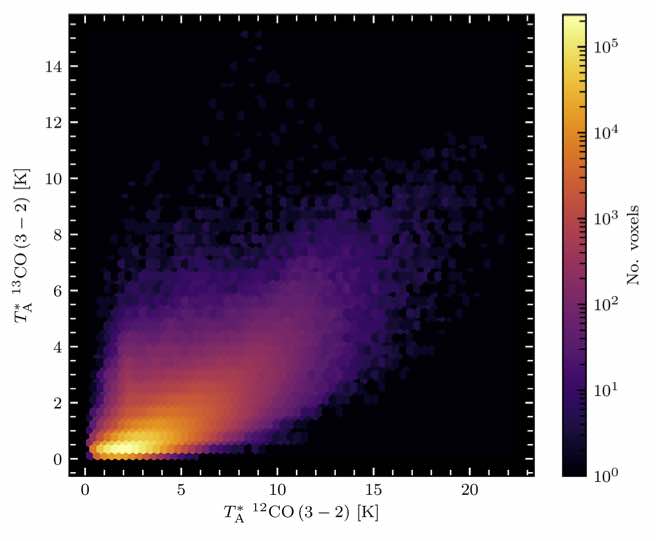
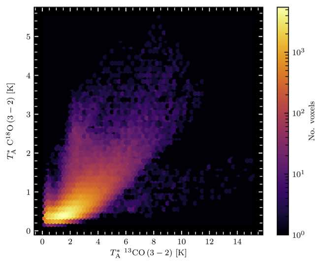
Figure 1: Comparisons of brightness temperatures used to determine observing thresholds for CHIMPS2. Left panel: ¹²CO and ¹³CO $J=3\rightarrow 2$ from COHRS and CHIMPS, respectively, used to select the detection threshold of ¹³CO for the Outer Galaxy segment. Right panel: ¹³CO and C¹⁸O from CHIMPS used to select the detection threshold of C¹⁸O for the CMZ segment.

The final segment of CHIMPS2 covers the CMZ between longitudes of $\ell$ = $\pm$5$\degr$ in the latitude range of $\mid\,$b$\,\mid$ $<$ 0$\aas@@fstack{\circ}$50. This range covers the 850-$\upmu$m continuum emission presented in Parsons et al. (2018). The extended velocity range of $\sim$ 550 km s^-1 present in the CO emission from the Galactic Centre (Dame et al., 2001), requires the use of the 1-GHz bandwidth mode of HARP. In this mode, ¹³CO and C¹⁸O cannot be observed simultaneously. Therefore, the ¹³CO is observed as a blind survey, while C¹⁸O data are taken as follow-up observations towards areas determined from the brightness-temperature relationship from CHIMPS (Rigby et al., 2016), displayed in the right panel of Fig. 1. A ¹³CO brightness-temperature threshold of 3 K was adopted.

The longitude coverage of the CHIMPS, CHIMPS2, and COHRS surveys are shown in Fig. 2. The FUGIN and SEDIGISM surveys are included due to the complementary nature of their observations. The CHIMPS2 latitude coverage in the Outer Galaxy follows that of Hi-GAL (Molinari et al., 2016) and is shown in Fig. 3, where the FUGIN survey latitude range is also displayed.

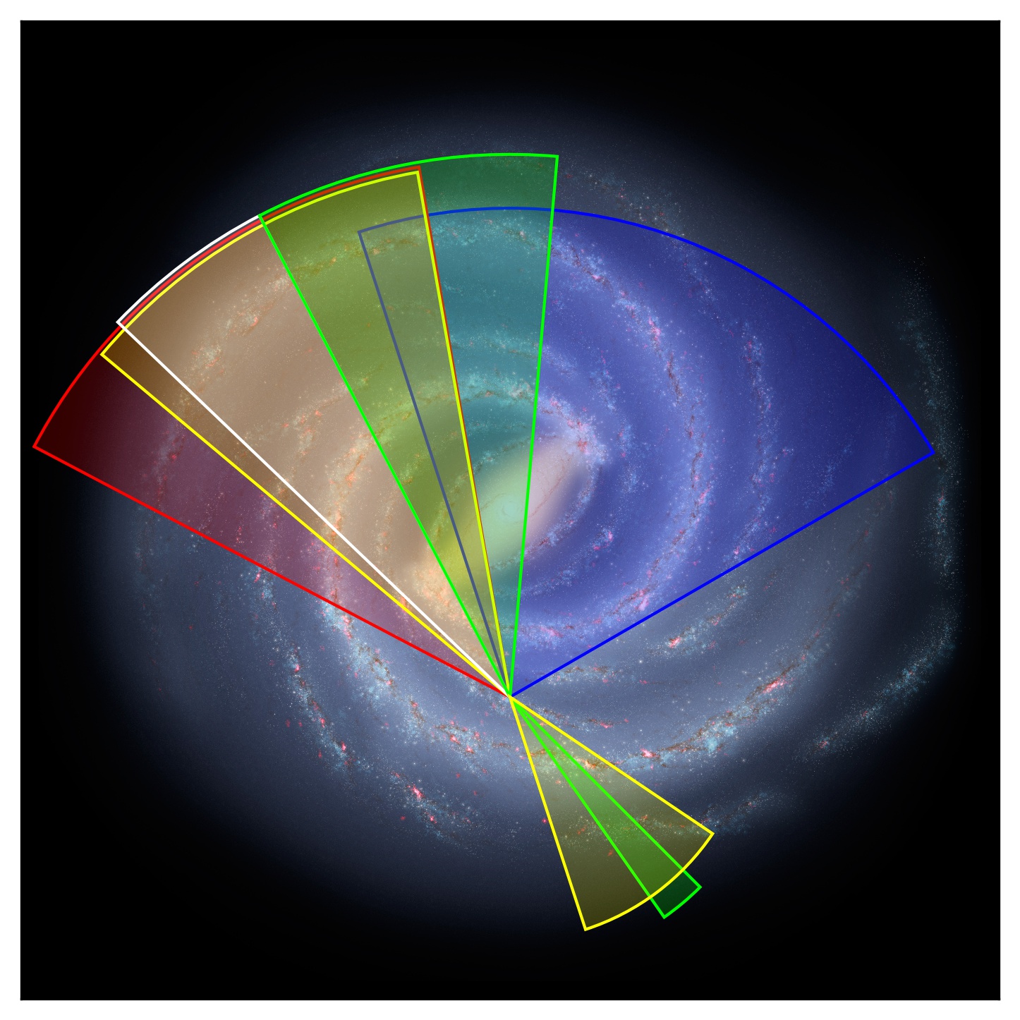
Figure 2: The area of the Galaxy covered by the CHIMPS2 survey (green segments). Complementary surveys are shown for comparison of their longitude coverage, COHRS (red), CHIMPS (white), yellow (FUGIN), and SEDIGISM (blue). The background image is the artist’s impression of the Milky Way by Robert Hurt of the Spitzer Science Center, made in collaboration with Robert Benjamin.

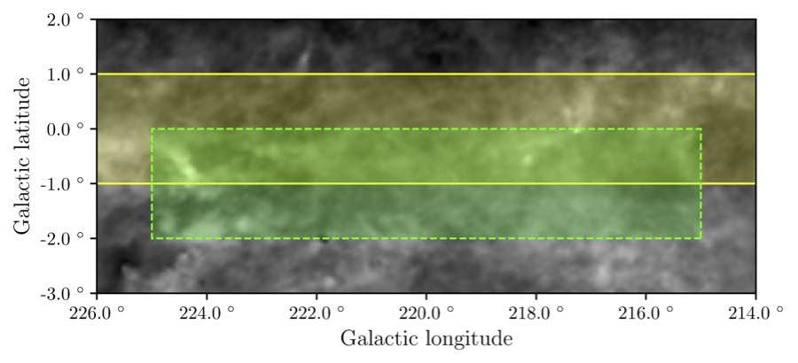
Figure 3: The area of the Outer Galaxy covered by CHIMPS2 (green dashed) and FUGIN (yellow). FUGIN is extended to longitudes of $\ell$ = 198$\degr$ to $\ell$ = 236$\degr$. Hi-GAL covers the same area as CHIMPS2. The background image is the Planck dust opacity map (Planck Collaboration et al., 2014).

2.2 Science Goals

The science goals of the CHIMPS2 project are multi-faceted, and intended to give us a greater understanding of the effect of environment on the star-formation process. The main goals are outlined below.

• Production of comparative samples of Galactic molecular clouds across a range of Galactic environments with cloud properties, analysed using complementary CO $J\,=\,1\rightarrow 0$ surveys such as FUGIN (Umemoto et al., 2017) and Milky Way Imaging Scroll Painting (MWISP; Gong et al. 2016; Su et al. 2019). Line-intensity ratios are found to be robust indicators of excitation conditions (e.g., Nishimura et al., 2015), with simulations validating these methods (Szűcs et al., 2014). Multi-transition models simulating observations, such as those of Peñaloza et al. (2017, 2018), will refine current LTE approximate methods (Rigby et al., 2019).

• Combine with Hi-GAL (Molinari et al., 2016; Elia et al., 2017), JCMT Plane Survey (JPS; Moore et al. 2015; Eden et al. 2017), ATLASGAL (Contreras et al., 2013; Urquhart et al., 2014), and other continuum data to map the SFE and DGMF in molecular gas and constrain the mechanisms chiefly responsible for the regulation of SFE. The dense-gas SFE is largely invariant on $\sim$ kpc scales in the Inner Galaxy disc (Moore et al., 2012; Eden et al., 2015) but falls significantly within the central 0.5 kpc (Longmore et al., 2013; Urquhart et al., 2013). Comparing these regions, along with the Outer Galaxy, where the metallicity is much lower (Smartt & Rolleston, 1997), and the bar-swept radii will increase our understanding of the impact of environment on the star-formation process. Variations within the CMZ may also provide insight into high-redshift star formation, since the physical condition of the clouds in this region are similar to those in galaxies at $z\,\sim\,2-3$ (Kruijssen & Longmore, 2013).

• Analyse the turbulence within molecular clouds and its relationship to the large variations in SFE and DGMF/CFE between one cloud and another (Eden et al., 2012; Eden et al., 2013, 2015). The ratio of compressive to solenoidal turbulence in molecular clouds to the CFE and SFE may determine how the internal physics of molecular clouds is altering the star formation (Brunt & Federrath, 2014; Federrath et al., 2016; Orkisz et al., 2017).

• Determine Galactic structure as traced by molecular gas and star formation, and the relationship between the two. The CHIMPS survey found significant, coherent, inter-arm emission (Rigby et al., 2016), identified as a connecting spur (Stark & Lee, 2006) of the type identified in external systems (e.g. Elmegreen, 1980).

• Use comparable neutral-hydrogen data (e.g., THOR; Beuther et al. 2016) to constrain cloud-formation models and relate turbulent conditions within molecular clouds to those in the surrounding neutral gas. The first stage of the macro star-formation process is the conversion of neutral gas into molecular gas, and therefore, clouds (Wang et al., 2020). The comparison of the THOR survey with CHIMPS2 data will allow estimates of the efficiency of this process, as well as the underlying formation process (e.g. Bialy et al., 2017) to be made.

• Study the relationship of filaments to star formation, and of gas flow within filaments to accretion and mass accumulation in cores and clumps. The filaments in question cover different scales. Several long ($>$ 50 pc) filamentary structures have been identified (Ragan et al., 2014; Zucker et al., 2015), and the CHIMPS2 data will allow for a determination of how much molecular gas is contained within these structures. On smaller scales, Herschel observations have shown a web of filamentary structures (e.g. André et al., 2010; Schisano et al., 2014) in which star-forming clumps are hosted (Molinari et al., 2010b). The gas flow into these clumps can be traced by the high-resolution CHIMPS2 data (e.g. Liu et al., 2018).

• Test current models of the gas kinematics and stability in the Galactic-centre region, the flow of gas from the disc, through the inner 3 kpc region swept by the Galactic Bar and into the CMZ. Models of the gas flows into the centres of galaxies give signatures of these flows (e.g Krumholz et al., 2017; Sormani et al., 2019; Armillotta et al., 2019; Tress et al., 2020), and the CHIMPS2 data can determine the mass-flow rate, the nature of the flows and the star-forming properties of these clouds.

3 Data and Data Reduction

The data reduction for the ¹²CO component of the CHIMPS2 survey broadly followed the approach used for COHRS (Dempsey et al., 2013), namely using the REDUCE_SCIENCE_NARROWLINE recipe of the orac-dr automated pipeline (Jenness & Economou, 2015), and employing the techniques described by Jenness et al. (2015). The pipeline invoked the Starlink applications software (Currie et al., 2014), including orac-dr, from its 2018A release. However, some new or improved orac-dr code was developed to address specific survey needs.

Since the original COHRS reductions were completed, many improvements have been made to the reduction recipe, yielding better-quality products. These include automated removal of emission from the reference (off-position) spectrum that appear as absorption lines in the reduced spectra and can bias baseline subtraction, flat fielding using a variant of the Curtis et al. (2010) summation method, and masking of spectra affected by ringing in Receptor H07 (Jenness et al., 2015).

The reduced spectral (position, position, velocity) cubes were re-gridded to 6-arcsec spatial pixels, convolved with a 9-arcsec Gaussian beam, resulting in 16.6-arcsec resolution. This produces an improvement on existing ¹²CO $(J\,=\,3\rightarrow 2)$ data (e.g. Oka et al., 2012). Cubes with both the ‘native’ spectral resolution and $\Delta V=1$ km s ^-1 were generated. The cleaning came first because it included the identification and masking of spectra that contained some extraneous signal comprising alternate bright and dark spectral channels. A first-order polynomial was used to fit the baselines (aligning with COHRS; Dempsey et al. 2013), although in the CMZ half of the baselines did require fourth-order polynomials.

The reduction of each map was made twice. The first pass used fully automated emission detection and baseline fitting, or adopted the recipe parameters of an abutting reduced tile. A visual inspection of the resultant spectral cube, tuning through the velocities and plotting the tile’s integrated spectrum, enabled refined baseline and flat-field velocity range recipe parameters to be set. Also, any residual non-astronomical artefacts from the raw time series not removed in the quality-assurance phase of the reductions, and contamination from the off-position spectrum were assessed. In some cases of the former, such as transient narrow spikes, these were masked in the raw data before the second reduction. Approximately 7 per cent of the tiles exhibited reference emission, which was removed by ORAC-DR using an algorithm that will be described in a forthcoming paper on the COHRS Second Release (Park et al., in preparation). The off-positions employed in the CHIMPS2 CMZ data are listed in Table 3.

Only 2 of 75 ¹²CO CMZ tiles could not be flat fielded. In the best-determined flat fields, the corrections were typically less than 3 percent, although receptor H11 was circa 8 per cent weaker than the reference receptor. Example sets of recipe parameters are given in Appendix A.

All intensities given in this paper are on the $T_{\mathrm{A}}^{*}$ scale. To convert this to the main-beam temperature scale, $T_{\mathrm{mb}}$, use the following relation $T_{\mathrm{mb}}\,=\,T_{\mathrm{A}}^{*}/\upeta_{\mathrm{mb}}$, where $\upeta_{\mathrm{mb}}$ is the main detector efficiency and has a value of 0.72 (Buckle et al., 2009).

Table 3: The off positions for the CMZ observations in the CHIMPS2 survey.

Galactic	Galactic
Longitude ($\degr$)	Latitude ($\degr$)
$-$2.50	2.50
0.78	$-$2.75
2.60	$-$2.50
3.00	$-$2.50
5.00	2.50

4 Results: ¹²CO in the CMZ

We are presenting the first results from the CHIMPS2 survey. These are the ¹²CO $J\,=\,3\rightarrow 2$ emission within the CMZ. They provide a first look at the potential science that can be achieved with such data, which have greater resolution and/or trace higher densities than other large-scale CO surveys of the CMZ across the transition ladder ($J\,=\,1\rightarrow 0$; Bally et al. 1987; Oka et al. 1998; Dame et al. 2001; Barnes et al. 2015; $J\,=\,2\rightarrow 1$; Schuller et al. 2017; $J\,=\,3\rightarrow 2$; Oka et al. 2012). The data will be combined with the corresponding CHIMPS2 ¹³CO $J\,=\,3\rightarrow 2$ results in a future release, along with a kinematic and dynamic analysis of the CO-traced molecular gas in the CMZ.

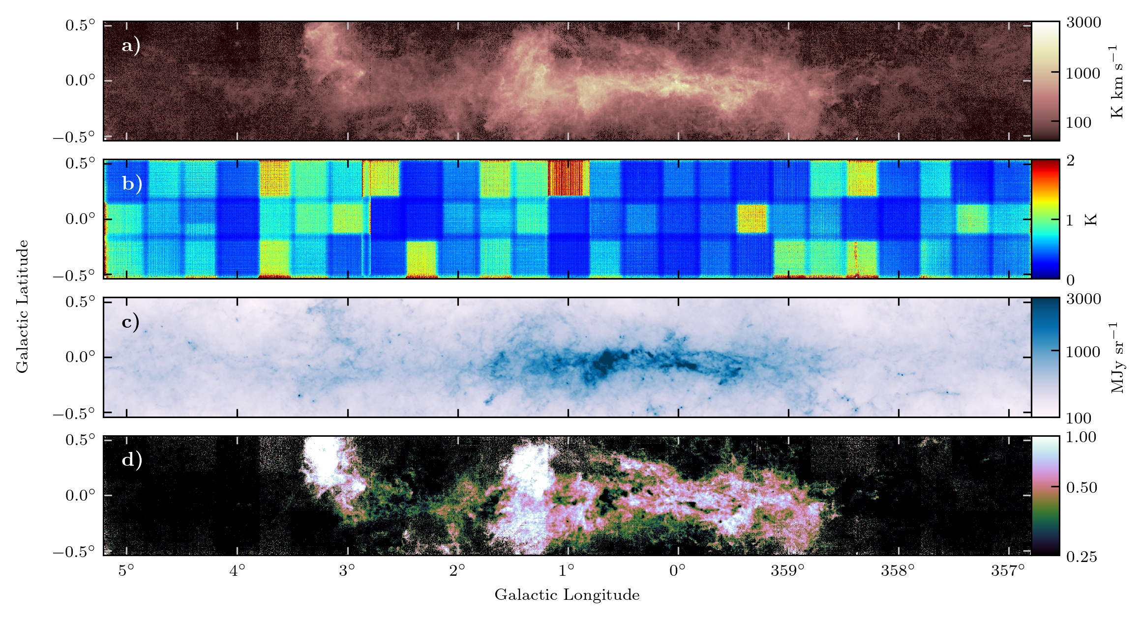
Figure 4: (a) The integrated emission from the ¹²CO $J\,=\,3\rightarrow 2$ CMZ data obtained as of October 2018. Each spectrum was integrated over all velocity channels; (b) Variance map of the ¹²CO $J\,=\,3\rightarrow 2$ CMZ data displayed in (a); (c) Herschel 500-$\upmu$m surface-brightness distribution from the Hi-GAL survey (Molinari et al., 2016); (d) CMZ ratio of ¹²CO $J\,=\,3\rightarrow 2$ integrated intensity (a) to Herschel Hi-GAL 500-$\upmu$m surface brightness (c).

4.1 Intensity distribution

Panel (a) of Fig. 4 shows the map of integrated intensity of ¹²CO $J\,=\,3\rightarrow 2$ in the CMZ region between $\ell=357^{\circ}$ and $\ell=+5^{\circ}$, $|\,b\,|\leq$ 0$\aas@@fstack{\circ}$5, constructed from data obtained up to the end of 2018. Panel (b) of Fig. 4 shows the ¹²CO $J\,=\,3\rightarrow 2$ intensity variance array mosaic and hence the relative noise levels in each constituent tile within the CMZ survey region.

A histogram of the voxel values of the map in Panel (a) of Fig. 4 is displayed in the top panel of Fig. 5. The distribution is modelled by a Gaussian function with a mean of 0.05 K and a standard deviation of 0.58 K. The data distribution departs from the Gaussian in the negative wing due to non-Gaussian noise and non-uniform noise across the data set. In the positive wing, the excess comes from the real emission and the aforementioned noise. A histogram of the rms noise values from the variance maps in Panel (b) of Fig. 4 are displayed in the bottom panel of Fig. 5. Each pixel in these variance maps represents one complete spectrum from the data cube. The values in the histogram are the square root of those in the map, giving the standard deviation. The distribution peaks at 0.38 K, comparable with the value obtained from the Gaussian fit in the emission in the top panel of Fig. 5.

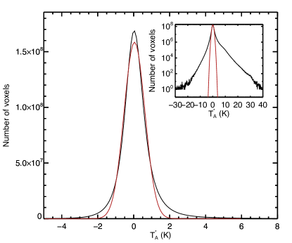
Figure 5: Top panel: histogram of all voxels in Panel (a) of Fig. 4. The red lines display the result of a Gaussian fit to the distribution. The inset shows the distribution and Gaussian fit on a logarithmic scale. Bottom panel: histogram of the noise values in Panel (b) of Fig. 4. The double bump is due to the differing observing conditions across the map, as seen in Dempsey et al. (2013). The inset shows the same distribution on a logarithmic scale.

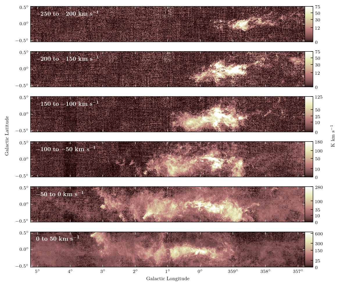
Figure 6: The integrated emission of the map, split into 50-km s^-1 channels. The top map is $-$250 to $-$200 km s^-1; the second map is $-$200 to $-$150 km s^-1; the third map is $-$150 to $-$100 km s^-1; the fourth map is $-$100 to $-$50 km s^-1; the fifth map is $-$50 to 0 km s^-1; and the bottom map is 0 to 50 km s^-1.

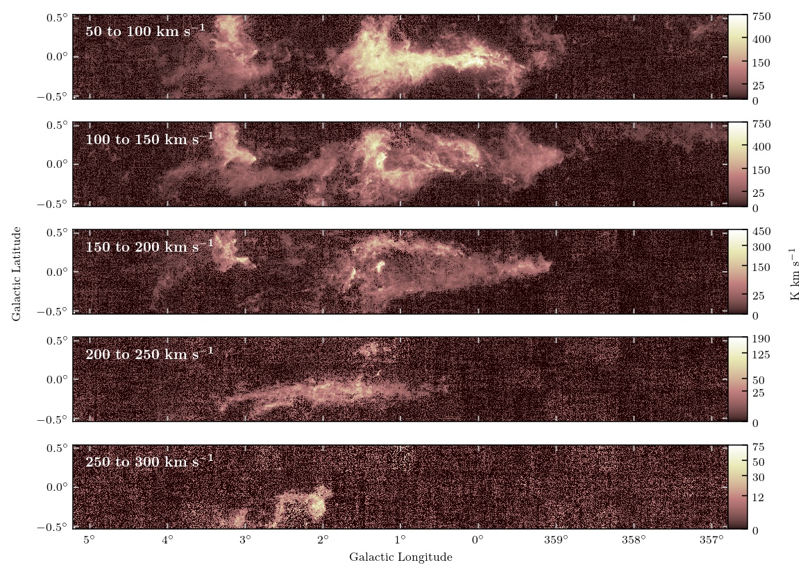
Figure 7: The integrated emission of ¹²CO $J=3\rightarrow 2$, split into 50-km s^-1 channels. From top to bottom, these are 50 to 100 km s^-1; 100 to 150 km s^-1; 150 to 200 km s^-1; 200 to 250 km s^-1; 250 to 300 km s^-1.

500-$\upmu$m continuum-emission data from the Herschel Hi-GAL project (Molinari et al., 2010a, 2011b) at 37-arcsec resolution are displayed in Panel (c) of Fig. 4. Panel (d) of Fig. 4 shows the distribution of the ratio of ¹²CO $J\,=\,3\rightarrow 2$ integrated intensity to 500-$\upmu$m continuum surface brightness. The ratio values (while arbitrary) range from $\sim$ 0.1 to 2.0 – a factor of $\sim$20.

Figs. 6 & 7 show the ¹²CO $J\,=\,3\rightarrow 2$ emission integrated over 50-km s^-1 velocity windows within the range $-$250 km s^-1 to 300 km s^-1, with no emission detected at velocities lower than $-$250 km s^-1.

Fig. 8 is the same as Panel (d) in Fig. 4 but with the longitude range limited to $\ell\,=\,-1\degr$ to $1\aas@@fstack{\circ}7$. A number of compact minima coincident with bright regions in both the continuum and CO-line maps can be seen by eye and appear to represent high column-density objects in which the CO emission is reduced due to, e.g. high optical depth. In order to produce an objective list of these sources, we applied the CuTEx object-detection package (Molinari et al., 2011a, 2017) to the inverted (reciprocal) ratio image. CuTEx was chosen as it was designed to deal with extended backgrounds in Herschel data. The detection thresholds were four times the rms noise in the second derivative (curvature) data and a minimum of four contiguous pixels. The resulting sample was then filtered to remove sources smaller than 35 arcsecs in either axis, to represent the 500-$\upmu$m Herschel beam size. The detected sources are marked in Fig. 8 as cyan squares and listed in Table 4.

As can be seen, not all the visible compact minima were detected by CuTEx, including several well-known sources. Table 4 lists several of the latter that can be picked out in Fig. 8, including The Brick ($\ell\simeq 0\aas@@fstack{\circ}25$), the clouds of the dust ridge at $\ell=0\aas@@fstack{\circ}3$–$0\aas@@fstack{\circ}5$, Sgr B2 at $\ell\simeq 0\aas@@fstack{\circ}7$, the 50- and 20-km s^-1 clouds at $\ell=359\aas@@fstack{\circ}9$ – $360\aas@@fstack{\circ}0$, Sgr C at $\ell\simeq 359\aas@@fstack{\circ}4$, as well as the southern part of the loop structure discussed by Molinari et al. (2011b), Henshaw et al. (2016) and others, in terms of clouds orbiting the central potential. The known objects from Table 4 that were not detected by CuTEx, are plotted in Fig. 8 as white circles. In addition to these two sets of objects, there are at least as many that can be picked out by eye. This simple analysis thus has considerable potential as a discovery channel for finding previously unknown dense, compact sources in such data and will be investigated further in future work. Here, we briefly investigate whether or not such sources tend to be colder than their surroundings.

The source extraction with CuTEx was repeated on the data in Fig. 8 but, rather than the reciprocal map above, now the maxima were detected. The positions of both CuTEx samples were used to extract temperature and column densities from the results of Marsh et al. (2017), produced by the ppmap procedure outlined in Marsh et al. (2015). The left panel of Fig. 9 shows the total column density contained within the sources at each temperature within the ppmap grid. There are 12 temperatures, evenly separated in log space between 8 K and 50 K. The peak total column density is found at 18.4 K for the minima, compared with 21.7 K for the maxima. The positions of the same sources were used to extract values from the column-density-weighted mean temperature maps produced by PPMAP, and the cumulative distributions of these values are shown in the right panel of Fig. 9.

The distribution of temperatures at the positions of the ¹²CO/500$\,\upmu$m minima in Fig. 8 is weighted to lower values than that of the maxima. The former are therefore tracing denser, colder structures, probably with high optical depths in ¹²CO and perhaps some degree of freeze-out of CO molecules onto dust grains. The minima generally form quite compact features that pick out many of the dense clouds studied by, e.g., Walker et al. (2018). By induction, high values, which tend to be extended, should therefore correspond to warmer areas of low ¹²CO optical depth.

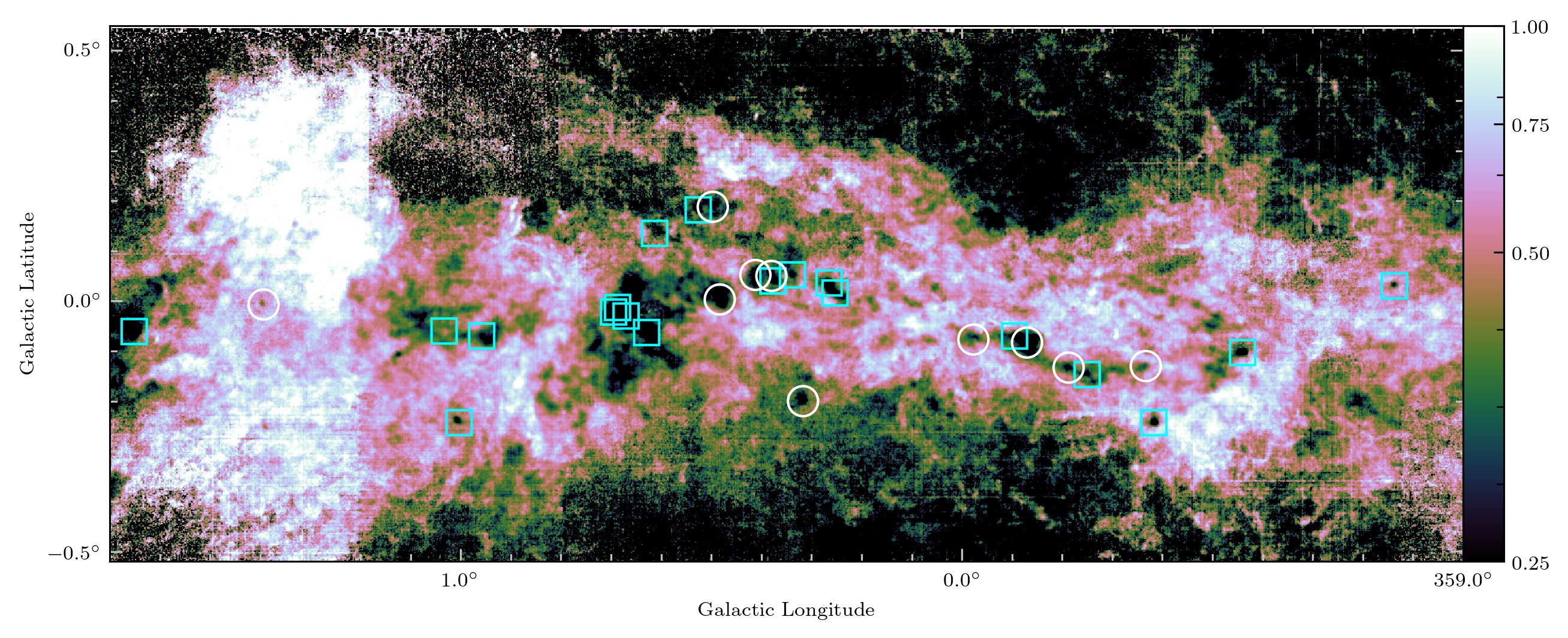
Figure 8: A close-up of the central portion of Panel (d) of Fig. 4. The cyan squares are compact sources detected at 4-sigma significance using CuTEx. The white circles are at the positions of several known dense clouds or clumps. Both samples are included in Table 4.

Table 4: Known compact sources in the ¹²CO/500-$\upmu$m ratio map (Fig. 8). Sources labelled with an asterisk were also detected by CuTEx.

Galactic	Galactic	Source Name and Notes	Reference
Longitude ($\degr$)	Latitude ($\degr$)
359.137	+0.030	*H ii region; MMB G359.138+00.031	Walsh et al. 1998; Caswell et al. 2010
359.440	$-$0.103	*Sgr C	Tsuboi et al. 1991
359.617	$-$0.243	*BGPS G359.617-00.243; MMB G359.615-00.243	Caswell et al. 2010; Rosolowsky et al. 2010
359.633	$-$0.130	BGPS G359.636-00.131	Rosolowsky et al. 2010
359.750	$-$0.147	*AGAL G359.751-00.144	Contreras et al. 2013
359.787	$-$0.133	JCMT SCUBA source; BGPS G359.788-00.137	Di Francesco et al. 2008; Rosolowsky et al. 2010
359.870	$-$0.083	20-km s-1 cloud: UCH ii regions and H2O maser	Downes et al. 1979; Sjouwerman et al. 2002
359.895	$-$0.070	*AGAL G359.894$-$00.067	Contreras et al. 2013
359.977	$-$0.077	50-km s-1 cloud: UCH ii regions and H2O maser	Ekers et al. 1983; Reid et al. 1988
0.253	+0.016	*The Brick	Longmore et al. 2012
0.265	+0.036	*AGAL G000.264+00.032	Contreras et al. 2013
0.317	$-$0.200	AGAL 0.316-0.201; MMB	Urquhart et al. 2013
0.338	+0.052	*Dust-ridge b	Lis et al. 1999
0.377	+0.040	*MMB G000.376+00.040; BGPS G000.378+00.041	Caswell et al. 2010; Rosolowsky et al. 2010
0.380	+0.050	Dust-ridge c	Lis et al. 1999
0.412	+0.052	Dust-ridge d & BGPS G000.414+00.051	Lis et al. 1999; Rosolowsky et al. 2010
0.483	+0.003	Sgr B1-off: UCH ii regions and H2O maser	Lu et al. 2019
0.497	+0.188	MMB G000.496+00.188; BGPS G000.500+00.187	Caswell et al. 2010; Rosolowsky et al. 2010
0.526	+0.182	*AGAL 0.526+0.182	Contreras et al. 2013
0.613	+0.135	*2MASS J17463693$-$2820212	Cutri et al. 2003
0.629	$-$0.063	*AGAL G000.629$-$00.062	Contreras et al. 2013
0.670	$-$0.030	*Sgr B2: UCH ii regions	Ginsburg et al. 2018
0.687	$-$0.013	*JCMT SCUBA-2 source	Parsons et al. 2018
0.695	$-$0.022	*AGAL G000.693$-$00.026	Contreras et al. 2013
0.958	$-$0.070	*JCMT SCUBA-2 source	Parsons et al. 2018
1.003	$-$0.243	*Sgr D1	Liszt 1992
1.123	$-$0.110	*Sgr D UCHII + H2O	Downes & Maxwell 1966; Mehringer et al. 1998
1.393	$-$0.007	Sgr D8	Eckart et al. 2006
1.651	$-$0.061	* AGAL G001.647$-$00.062	Contreras et al. 2013

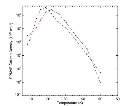
Figure 9: Left panel: the total column density found within the CuTEx sources in each temperature slice from the PPMAP analysis of the CMZ (Marsh et al., 2017). The minima from Fig. 8 are represented by blue points, whereas the maxima are red. Right panel: the cumulative distribution of the temperature contained within the CuTEx in the column-density weighted PPMAP temperature maps. The minima are represented by the blue dashed line, whereas the maxima are the red dot-dash line.

4.2 Kinematic structure

4.2.1 High-velocity-dispersion features

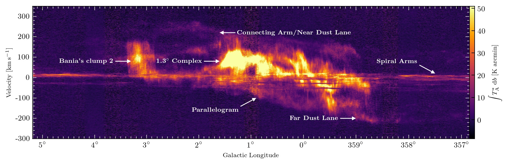
Figure 10: CMZ longitude-velocity map of ¹²CO $J\,=\,3\rightarrow 2$ intensity integrated over latitude from data complete as of Sept 2018.

Fig. 10 contains the $\ell-V_{\textnormal{LSR}}$ distribution of the ¹²CO $J\,=\,3\rightarrow 2$ intensity, integrated over the whole latitude range. The main features are labelled in Fig. 10 and are the parallelogram-like structure; Bania’s Clump 2; the Connecting Arm, the dust lanes fuelling the CMZ; and a series of supernova remnants.

The bright, high-velocity-dispersion emission between $\ell\simeq 358\aas@@fstack{\circ}5$ and $1\aas@@fstack{\circ}5$; $V_{\textnormal{LSR}}\sim\pm\,250$ km s^-1 in Fig. 10 that resembles a parallelogram (Bania, 1977; Bally et al., 1987; Morris & Serabyn, 1996) is thought to be caused by the dust lanes in the CMZ. The lateral sides are interpreted as the gas that is accreting onto the CMZ from the dust lanes (Sormani et al., 2019). The top and bottom sides are caused by gas that is partly accreting onto the CMZ after travelling past the dust lanes (Sormani et al., 2018). This, combined with the efficient conversion of atomic to molecular gas, causes the velocity structure that we observe in the CMZ (Sormani et al., 2015a).

The longitudinal asymmetry of this region of bright CO emission with respect to $\ell=0^{\circ}$, along with the velocity centroid offset of $\sim+40$ km s^-1 seen in Fig. 10, was previously explained as the result of gas responding to an asymmetry in the Galactic potential in $m=1$ mode oscillation with respect to the Galactic disc (e.g., Morris & Serabyn, 1996). However, the positional asymmetry has been recently suggested by Sormani et al. (2018) to be due to non-steady flow of gas in the bar potential. In these models, a combination of hydrodynamical and thermal instabilities mean that the gas flow into the CMZ is clumpy and unsteady. This structure leads to transient asymmetries in the inward flow, which we observe, the authors argue, as the longitudinal asymmetry in the gas distribution. Also, structures similar to those observed at the top and bottom edges of the parallelogram feature are detected in the simulations, where they correspond to far- and near-side shocks at the leading edges of the rotating bar. The bright compact structures within this structure are the molecular clouds on librations around $x_{2}$ orbits in a ring around the CMZ with semi-major axis $\sim 0.3$ kpc; and the several features that are narrow in $\ell$, but have large velocity dispersions, are shocks where the infalling material meets the CMZ or librations around an $x_{2}$ orbit (Kruijssen et al., 2015; Tress et al., 2020). The velocity offset is displayed in Fig. 11. This is the first-moment map of the sub-region in Fig. 8, created using the spectral-cube package (Ginsburg et al., 2019) and reflecting the centroid velocity at each pixel.

Figure 11: First moment map of the ¹²CO CMZ map in the region represented in Fig. 8.

Bania’s Clump 2 can be seen as a high-velocity-dispersion cloud in Fig. 10 at $\ell$ = 3$\aas@@fstack{\circ}$2 (Bania, 1977). The line width of Bania’s Clump 2 appears to cover over 100 km s^-1 (Stark & Bania, 1986), with very narrow longitude coverage (Liszt, 2006) but high-resolution data have found that the velocity range is made up of many lower-linewidth components (Longmore et al., 2017). Clouds such as these are the signature of shocks as clouds collide with the dust lane, as opposed to the turbulence of individual clouds (Sormani et al., 2015b, 2019). Another high-velocity-dispersion cloud present in Fig. 10 is the $\ell$ = 1$\aas@@fstack{\circ}$3 complex (Bally et al., 1988; Oka et al., 1998). The high-velocity dispersion has three potential causes. The first is a series of supernova explosions (Tanaka et al., 2007), with the alternatives reflecting the acceleration of gas flows along magnetic field lines due to Parker instabilities (Suzuki et al., 2015; Kakiuchi et al., 2018) or collisions between gas on the dust lanes and the gas orbiting the CMZ (Sormani et al., 2019). Neither of these two structures shows signatures of ongoing star formation (Tanaka et al., 2007; Bally et al., 2010), with no associated 70-$\upmu$m Hi-GAL compact sources (Elia et al., 2017), which are considered to be a signature of active star formation (Ragan et al., 2016, 2018).

The Connecting Arm (Rodriguez-Fernandez et al., 2006) is also visible in the $\ell-V_{\textnormal{LSR}}$ diagram. Though described as a spiral arm, it is in fact a dust lane at the near side of the CMZ (e.g. Fux, 1999; Marshall et al., 2008; Sormani et al., 2018), with a symmetrical dust lane found at the far side of the CMZ. We also see the latter in Fig. 10 as the curved feature at $V_{\textnormal{LSR}}\sim-200$ km s^-1 running between $\ell\simeq 359^{\circ}$ and $357^{\circ}$. These dust lanes are signatures of accretion into the CMZ (Sormani & Barnes, 2019), fuelling episodic star formation in this region (Krumholz et al., 2017).

We also confirm the findings of Tanaka (2018) and Reid & Brunthaler (2020), who observed no evidence of an intermediate-mass black hole (IMBH) at the position of $\ell\,=\,-0\aas@@fstack{\circ}40$, $\emph{b}\,=\,-0\aas@@fstack{\circ}22$ (Oka et al., 2016; Oka et al., 2017). Fig. 12 shows the $\ell-V_{\textnormal{LSR}}$ ¹²CO intensity distribution of the observed tile that would contain this IMBH. There are no large-velocity-dispersion features that are indicative of an accreting IMBH being present in the $\ell-V_{\textnormal{LSR}}$ maps.

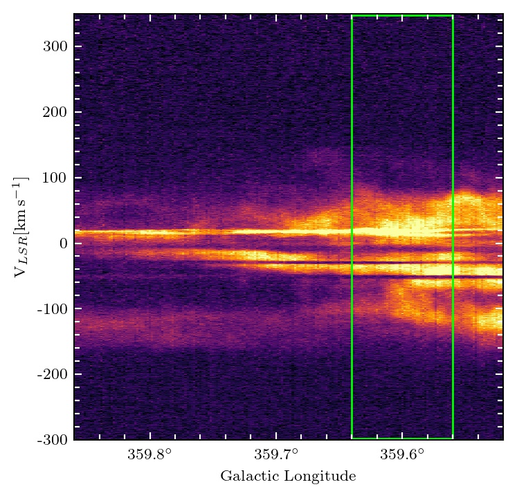
Figure 12: Longitude-velocity map of the individual ¹²CO tile containing the reported position of the IMBH CO$-$0.40$-$0.22 (Oka et al., 2016; Oka et al., 2017). The expected longitude range is marked by the green rectangle.

4.2.2 Foreground features

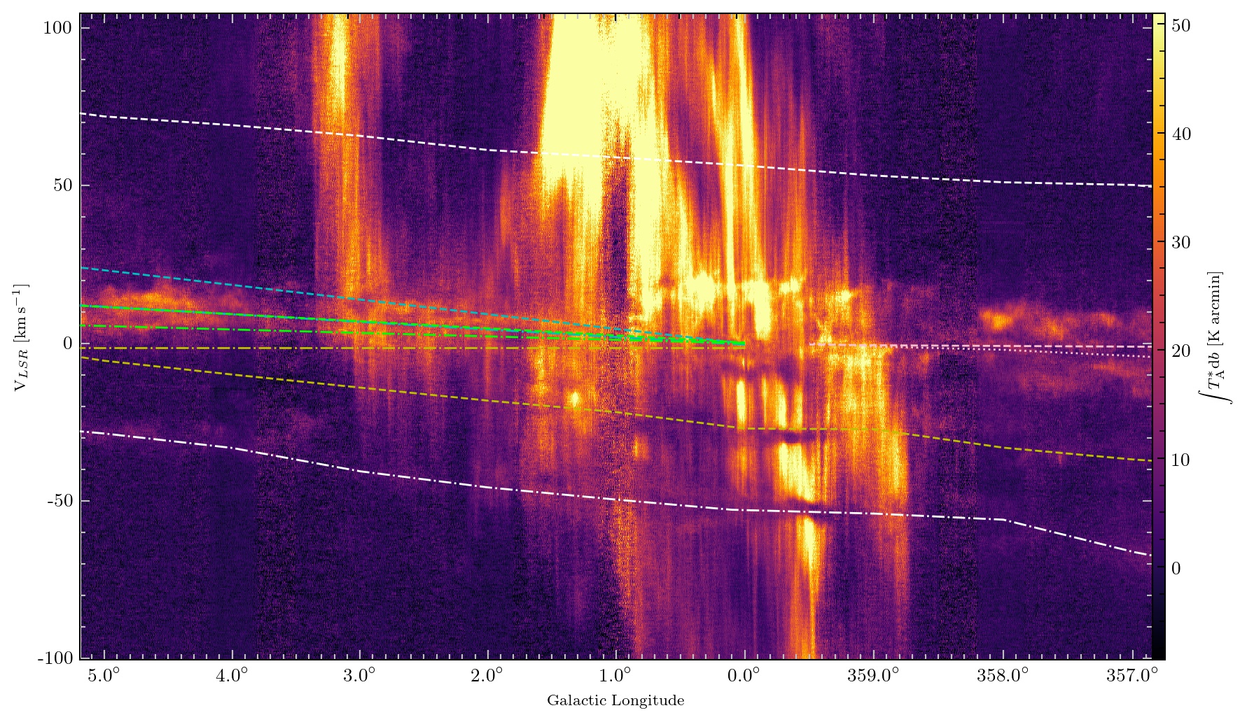
Figure 13: As in Fig. 10 but with the spiral arms of Reid et al. (2016) overlaid and the velocity range restricted to $V_{\textnormal{LSR}}\,\pm\,100$ km s^-1. The arm segments are labelled as follows: 3-kpc near and far arms (3kN, 3kF; white dashed and white dot-dash, respectively), Carina near portion (CrN; pink dashed), Centaurus-Crux near (CtN; pink dotted), Norma or 4-kpc (Nor; yellow dashed), Outer (Out; yellow dotted), Perseus (Per; blue dotted), Scutum near and far portions (ScN, ScF; blue dot-dash and blue dashed, respectively), and Sagittarius near and far portions (SgN, SgF; green dot-dash and green dashed, respectively). The Connecting Arm is out of this velocity range whilst the Outer Scutum-Centaurus, Carina far, an extension of the Connecting Arm, and Centaurus-Crux far arm segments currently have no parallax measurements and are not plotted.

The $\ell-V_{\textnormal{LSR}}$ plot (Fig. 10) also shows several clear features with narrow velocity widths, in absorption and emission, probably corresponding to foreground structures, namely spiral arms. We can use these features to constrain the loci of these arms as they cross the CMZ. Several of the arm features modelled in Reid et al. (2016) are plotted on the same data, restricted to $V_{\textnormal{LSR}}\,\pm\,100$ km s^-1, in Fig. 13.

At the $\ell=0\degr$ position, there are three features in absorption at $V_{\textnormal{LSR}}\simeq-60$, $-30$ and $-10$ km s^-1, with one emission feature at $\sim+10$ km s^-1. All of these appear to have substructure and possibly shallow gradients and are somewhat discontinuous across the longitude range. Following Bronfman et al. (2000) and Sanna et al. (2014), we can postulate that the $-$60 km s^-1 feature is the near 3-kpc arm and the $-$30 km s^-1 feature is the Norma arm.

To identify these features, more-precise $\ell-V_{\textnormal{LSR}}$ plots were made, integrating over the latitude and velocity range identified for these arms in Reid et al. (2016). Fig. 14 displays the $\ell-V_{\textnormal{LSR}}$ plots for the near 3-kpc arm, far 3-kpc arm, Norma arm, Perseus arm, and the far Sagittarius arm. The latitude and velocity ranges of the five spiral arms are: $\pm$ 0$\aas@@fstack{\circ}$2 and $-$80 to $-$20 km s^-1, $\pm$ 0$\aas@@fstack{\circ}$1 and 30 to 80 km s^-1, $\pm$ 0$\aas@@fstack{\circ}$2 and $-$50 to 10 km s^-1, $-$0$\aas@@fstack{\circ}$1 to 0$\degr$ and $-$30 to 30 km s^-1, and $-$0$\aas@@fstack{\circ}$1 to 0$\degr$ and $-$10 to 50 km s^-1, for the near 3-kpc, far 3-kpc, Norma, Perseus, and far Sagittarius arms, respectively.

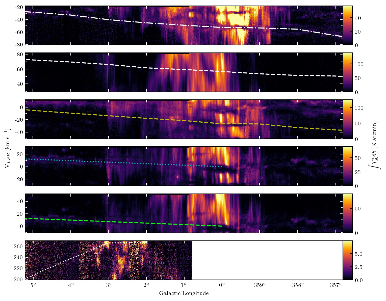
Figure 14: Longitude-velocity maps isolated over the latitude and velocity range identified by Reid et al. (2016). Top panel: near 3-kpc arm. Second panel: far 3-kpc arm. Third panel: Norma spiral arms. Fourth panel: Perseus spiral arm. Fifth panel: far Sagittarius spiral arm. Bottom panel: Connecting Arm, which is limited to a longitude range of $\ell\,>\,0\aas@@fstack{\circ}8$. The overlaid lines are the loci of the relevant spiral arms.

The $\ell-V_{\textnormal{LSR}}$ plots for the near 3-kpc arm and the Norma arm confirm the detection of these spiral arms. The near-3kpc arm displays absorption in the CMZ region, with emission detected in positive longitudes. The Norma spiral arm is detected in absorption. There is no evidence in these data of the far 3-kpc arm, that Sanna et al. (2014) suggest crosses $\ell=0\degr$ at +56 km s^-1.

The Perseus spiral arm and the far segment of the Sagittarius arm both have emission that corresponds to the loci of these arms, in the positive longitudes at velocities $V_{\textnormal{LSR}}\simeq+10$ km s^-1. We are, therefore, unable to confirm which of these spiral arms we have detected.

We have also produced the $\ell-V_{\textnormal{LSR}}$ plot for the Connecting Arm, using the Reid et al. (2016) latitude and velocity ranges of $-$0$\aas@@fstack{\circ}$5 to 0$\aas@@fstack{\circ}$3 and 200 to 270 km s^-1. We detect this structure, the near-side dust lane down which material streams from distances of 3 kpc into the CMZ (e.g Cohen & Davies, 1976; Rodriguez-Fernandez et al., 2006; Sormani & Barnes, 2019).

In future work, we will extract the detected narrow arm features from the ¹²CO data cubes in order to analyse the molecular-gas properties within them and to allow kinematic analysis of the kinematics of the residual high-velocity-dispersion emission in the CMZ itself.

5 Summary

We introduce the CO Heterodyne Inner Milky Way Plane Survey (CHIMPS2). CHIMPS2 will complement the CHIMPS (Rigby et al., 2016) and COHRS (Dempsey et al., 2013) surveys by observing the Central Molecular Zone (CMZ), a segment of the Outer Galaxy, and to connect the CMZ to the current CHIMPS and COHRS observations in ¹²CO, ¹³CO, and C¹⁸O $(J\,=\,3\rightarrow 2)$ emission.

We present the ¹²CO $J\,=\,3\rightarrow 2$ data in the CMZ, covering approximately $-3\degr\,\leq\,\ell\,\leq\,5\degr$ and $\mid$b$\mid\,\leq\,0\aas@@fstack{\circ}50$. The data have a spatial resolution of 15 arcsec, a spectral resolution of 1 km s^-1 over velocities of $\mid$$V_{\textnormal{LSR}}$$\mid\,\leq$ 300 km s^-1, an rms of 0.58 K on 7.5 arcsec pixels and are available to download from the CANFAR archive.

Taking the ratio of the integrated-intensity to the 500-$\upmu$m continuum surface brightness from Hi-GAL, we find that the result correlates well with dust temperature. The minima tend to coincide with compact, dense, cool sources; whereas the maxima correspond to warmer, more-extended regions.

We investigate the kinematic structure of the CMZ data through the use of $\ell-V_{\textnormal{LSR}}$ plots. We are able to distinguish the high-velocity-dispersion features in the Galactic Centre, such as Bania’s Clump 2. We find no evidence for the existence of intermediate-mass black holes. We find evidence for spiral arms crossing in front of the Galactic Centre in both absorption and emission, detecting the near 3-kpc spiral arm, along with the Norma spiral arm, and evidence for emission in the space occupied by the far Sagittarius arm and the Perseus arm.

These data provide high-resolution observations of molecular gas in the CMZ, and will be a valuable data set for future CMZ studies, especially when combined with the future ¹³CO and C¹⁸O CHIMPS2 data. Further combination with the complimentary data sets from exisiting surveys in the molecular gas, such as SEDIGISM, and in the continuum from Hi-GAL and ATLASGAL will further increase the value.

Data Availability

The reduced CHIMPS2 ¹²CO CMZ data are available to download from the CANFAR archive. The data are available as mosaics, roughly 2$\degr$ $\times$ 1$\degr$ in size, as well as the individual observations. Integrated $\ell-\emph{b}$ and $\ell-V_{\textnormal{LSR}}$ maps, displayed in Section 5 for the whole CMZ are provided, as well as the $\ell-V_{\textnormal{LSR}}$ maps for the individual cubes. The data are presented in FITS format.

The raw data are also downloadable from the JCMT Science Archive hosted by the Canadian Astronomy Data Centre using the Project ID M17BL004.

Appendix A ORAC-DR parameters

The available recipe parameters are described in the REDUCE_SCIENCE_NARROWLINE documentation and summarised in the Classified Recipe Parameters appendix of Starlink Cookbook 20.

We first list the parameters that were constant throughout the survey and will be applied to all ¹²CO data in the CHIMPS2 survey. The following parameters controlled the creation of the spectral cubes with smurf:makecube (Chapin et al., 2013; Jenness et al., 2013), and the maximum size of input data before they were processed in chunks.

CUBE_WCS = GALACTIC
PIXEL_SCALE = 6.0
SPREAD_METHOD = gauss
SPREAD_WIDTH = 9
SPREAD_FWHM_OR_ZERO = 6
TILE = 0
CUBE_MAXSIZE = 1536

CHUNKSIZE = 12288

The following parameters controlled the creation of the longitude-velocity maps and spectral-channel re-binning for the tiling of a large number of tiles.

REBIN = 1.0
LV_IMAGE = 1
LV_AXIS = skylat
LV_ESTIMATOR = sum

To guide the automated rejection of spectra affected by artefacts extraneous noise the following parameters were used.

BASELINE_LINEARITY = 1
BASELINE_LINEARITY_LINEWIDTH = base
BASELINE_REGIONS = -406.8:-272.0,124.0:377.5
BASELINE_LINEARITY_MINRMS = 0.080
HIGHFREQ_INTERFERENCE = 1
HIGHFREQ_RINGING = 0
LOWFREQ_INTERFERENCE = 1
LOWFREQ_INTERFERENCE_THRESH_CLIP = 4.0

These too were constants, except BASELINE_LINEARITY_LINEWIDTH was sometimes set to a range to be excluded from the non-linearity tests if there was a single continuous section of emission, otherwise BASELINE_REGIONS was used inclusively. HIGHFREQ_RINGING was only enabled (set to 1) when ringing (Jenness et al., 2015) was present in HARP Receptor H07. LOWFREQ_INTERFERENCE_THRESH_CLIP was set higher – 6, 8, or 10 – as needed for ¹²CO observations in the CMZ.

The following three parameters controlled how the receptor-to-receptor flat field was to be determined. The responses are normalised to Receptor H05, except in 15 cases in where H05 had failed quality-assurance criteria and H10 was substituted. In three CMZ cases the index method was preferred, using well-determined flat ratios from the same night. The regions used to derive the flat field were estimated by averaging all the spectra in the first pass of a reduction, then tuning through border velocity channels until there was deemed to be sufficient signal that was not overly concentrated, typically when the mean flux exceeded 0.2 K.

FLATFIELD = 1
FLAT_METHOD = sum
FLAT_REGIONS = -87.0:54.0,90.0:190.0

For ¹²CO observations in the CMZ, the following parameters related to the baseline fitting were used.

BASELINE_METHOD = auto
BASELINE_ORDER = 1
FREQUENCY_SMOOTH = 25
BASELINE_NUMBIN = 128
BASELINE_EMISSION_CLIP = 1.0,1.3,1.6,2.0,2.5

In some cases the baseline order was required to be set to 4.

BASELINE_ORDER = 4

The velocity coverage of the output data products in the CMZ were determined to be $-$407 to 355, and assigned to the FINAL_LOWER_VELOCITY and FINAL_UPPER_VELOCITY parameters.

The velocity limits containing all identified emission with a margin for error were set by MOMENTS_LOWER_VELOCITY and MOMENTS_UPPER_VELOCITY to aid in the creation of moments’ maps, such the integrated emission.

The final set of parameters were only applicable when there was noticeable contamination from the reference (off-position).

CLUMP_METHOD = clumpfind
SUBTRACT_REF_EMISSION = 1
REF_EMISSION_MASK_SOURCE = both
REF_EMISSION_COMBINE_REFPOS = 1
REF_EMISSION_BOXSIZE = 19

Author affiliations:
¹Astrophysics Research Institute, Liverpool John Moores University, IC2, Liverpool Science Park, 146 Brownlow Hill, Liverpool, L3 5RF, UK
²East Asian Observatory, 660 North A’ohoku Place, Hilo, Hawaii 96720, USA
³RAL Space, STFC Rutherford Appleton Laboratory, Chilton, Didcot, Oxfordshire OX11 0QX, UK
⁴School of Physics and Astronomy, Cardiff University, Queen’s Buildings, The Parade, Cardiff CF24 3AA, UK
⁵Department of Physics, University of Alberta, Edmonton, AB T6G 2R3, Canada
⁶Purple Mountain Observatory and Key Laboratory of Radio Astronomy, Chinese Academy of Sciences, Nanjing 210034, People’s Republic of China
⁷Korea Astronomy and Space Science Institute, 776 Daedeokdae-ro, Yuseong-gu, Daejon 34055, Republic of Korea
⁸University of Science and Technology, Korea (UST), 217 Gajeong-ro, Yuseong-gu, Daejeon 34113, Republic of Korea
⁹European Southern Observatory, Karl-Schwarzschild-Strasse 2, D-85748 Garching bei München, Germany
¹⁰Institute of Astronomy and Department of Physics, National Tsing Hua University, 300, Hsinchu, Taiwan
¹¹Nobeyama Radio Observatory, National Astronomical Observatory of Japan, National Institutes of Natural Sciences, 462-2, Nobeyama, Minamimaki, Minamimaksu, Nagano 384-1305, Japan
¹²Department of Astronomical Science, School of Physical Science, SOKENDAI (The Graduate University for Advanced Studies), 2-21-1, Osawa, Mitaka, Tokyo 181-8588, Japan
¹³Centre for Astrophysics and Planetary Science, University of Kent, Canterbury CT2 7NH, UK
¹⁴Department of Physics & Astronomy, Kwantlen Polytechnic University, 12666 72nd Avenue, Surrey, BC, V3W 2M8, Canada
¹⁵Wartburg College, Waverly, IA 50677, USA
¹⁶Subaru Telescope, National Astronomical Observatory of Japan, National Institutes of Natural Sciences, 650 North A’ohoku Place, Hilo, HI 96720, USA
¹⁷Centre de Recherche en Astrophysique du Québec, Département de physique, de génie physique et d’optique, Université Laval, QC G1K 7P4, Canada
¹⁸Key Laboratory for Research in Galaxies and Cosmology, Shanghai Astronomical Observatory, Chinese Academy of Sciences, 80 Nandan Road, Shanghai 200030, People’s Republic of China
¹⁹Department of Astrophysics, Vietnam National Space Center (VNSC), Vietnam Academy of Science and Technology (VAST), 18 Hoang Quoc Viet, Ha Noi, Vietnam
²⁰School of Space Research, Kyung Hee University, 1732 Deogyeong-daero, Giheung-gu, Yongin-si, Gyeonggi-do 17104, Republic of Korea
²¹SUPA, School of Physics and Astronomy, University of St Andrews, North Haugh, St Andrews KY16 9SS, UK
²²National Astronomical Observatories, Chinese Academy of Sciences, 20A Datun Road, Chaoyang District, Beijing 100012, China
²³Key Laboratory of FAST, NAOC, Chinese Academy of Science, Beijing 100012, China
²⁴Max-Planck-Institut für Astronomie, Königstuhl 17, D-69117 Heidelberg, Germany
²⁵Division of Particle and Astrophysical Science, Graduate School of Science, Nagoya University, Furo-cho, Chikusa-ku, Nagoya, Aichi 464-8602, Japan
²⁶Department of Earth and Space Science, Graduate School of Science, Osaka University, 1-1, Machikaneyama-cho, Toyonaka, Osaka 560-0043, Japan
²⁷Astronomical Institute, Graduate School of Science, Tohoku University, Aoba, Sendai, Miyagi 980-8578, Japan
²⁸Centre for Astrophysics Research, School of Physics Astronomy & Mathematics, University of Hertfordshire, College Lane, Hatfield, Herts AL10 9AB, UK
²⁹SUPA, School of Science and Engineering, University of Dundee, Nethergate, Dundee DD1 4HN, U.K.
³⁰Department of Physics and Astronomy, University of Waterloo, Waterloo, ONN2L 3G1, Canada
³¹Department of Astronomy, Xiamen University, Xiamen, Fujian 361005, China
³²Institute of Astronomy and Astrophysics, Academia Sinica. 11F of Astronomy-Mathematics Building, AS/NTU No.1, Section 4, Roosevelt Rd, Taipei 10617, Taiwan
³³Department of Earth Sciences, National Taiwan Normal University, 88 Section 4, Ting-Chou Road, Taipei 11677, Taiwan
³⁴Department of Earth Science Education, Seoul National University (SNU), 1 Gwanak-ro, Gwanak-gu, Seoul 08826, Republic of Korea
³⁵Max-Planck-Institut für Extraterrestrische Physik, Giessenbachstrasse 1, D-85741 Garching bei München, Germany
³⁶Department of Physics and Astronomy, University of Calgary, 2500 University Drive NW, Calgary, Alberta T2N 1N4, Canada
³⁷Department of Astronomy, Faculty of Mathematics and Natural Sciences, Institut Teknologi Bandung, Jl. Ganesha 10, Bandung 40132 Indonesia
³⁸Institute of Astronomy, National Central University, Jhongli 32001, Taiwan
³⁹Physical Research Laboratory, Navrangpura, Ahmedabad, Gujarat 380009, India
⁴⁰SOFIA Science Center, Universities Space Research Association, NASA, Ames Research Center, Moffett Field, CA 94035, USA
⁴¹Xinjiang Astronomical Observatory, Chinese Academy of Sciences, 830011 Urumqi, China
⁴²IAPS-INAF, via Fosso del Cavaliere 100, I-00133 Rome, Italy
⁴³Department of Physics and Astronomy, The Open University, Walton Hall, Milton Keynes MK7 6AA, UK
⁴⁴Max-Planck-Institut für Radioastronomie, Auf dem Hügel 69, 53121 Bonn, Germany
⁴⁵Department of Physics and Astronomy, McMaster University, 1280 Main St. W, Hamilton, ON L8S 4M1, Canada
⁴⁶Astrophysics Group, School of Physics, University of Exeter, Stocker Road, Exeter EX4 4QL, UK
⁴⁷Department of Astronomy and Space Science, Chungnam National University, 99 Daehak-ro, Yuseong-gu, Daejeon 34134, Republic of Korea
⁴⁸Jodrell Bank Centre for Astrophysics, School of Physics and Astronomy, University of Manchester, Oxford Road, Manchester M13 9PL, UK
⁴⁹School of Physics and Astronomy, University of Leeds, Leeds LS2 9JT, UK
⁵⁰National Astronomical Observatory of Japan, 2-21-1, Osawa, Mitaka, Tokyo, 181-8588, Japan
⁵¹Department of Physics and Astronomy, Seoul National University, Seoul 151-747, Republic of Korea
⁵²Graduate School of Pure and Applied Sciences, University of Tsukuba, 1-1-1 Tennodai, Tsukuba, Ibaraki 305-8571, Japan
⁵³Tomonaga Center for the History of the Universe, University of Tsukuba, 1-1-1 Tennodai, Tsukuba, Ibaraki 305-8571, Japan
⁵⁴Department of Physics and Atmospheric Science, Dalhousie University, Halifax, NS B3H 4R2, Canada
⁵⁵Department of Physics, Institute of Science and Technology, Keio University, 3-14-1 Hiyoshi, Kohoku-ku, Yokohama, Kanagawa 223-8522, Japan
⁵⁶School of Fundamental Science and Technology, Graduate School of Science and Technology, Keio University, 3-14-1 Hiyoshi, Kohoku-ku, Yokohama, Kanagawa 223-8522, Japan
⁵⁷College of Material Science and Chemical Engineering, Hainan University, Hainan 570228, China
⁵⁸Key Laboratory of Modern Astronomy and Astrophysics, Nanjing University, Ministry of Education, Nanjing 210093, China
⁵⁹Instituto de Radioastronomía y Astrofísica, Universidad Nacional Autonóma de México, Antigua Carretera a Pátzcuaro # 8701 Ex-Hda., San José de la Huerta, Morelia, Michoacán, C.P. 58089, México
⁶⁰Radio Telescope Data Center, Center for Astrophysics, Harvard & Smithsonian, 60 Garden Street, Cambridge, MA 02138, USA
⁶¹Department of Astronomy, Peking University, 100871 Beijing, China
⁶²Department of Astronomy, Yunnan University, Key Laboratory of Astroparticle Physics of Yunnan Province, Kunming 650091, China

References

- André et al. (2010) André P., et al., 2010, A&A, 518, L102
- Armillotta et al. (2019) Armillotta L., Krumholz M. R., Di Teodoro E. M., McClure-Griffiths N. M., 2019, MNRAS, 490, 4401
- Bally et al. (1987) Bally J., Stark A. A., Wilson R. W., Henkel C., 1987, ApJS, 65, 13
- Bally et al. (1988) Bally J., Stark A. A., Wilson R. W., Henkel C., 1988, ApJ, 324, 223
- Bally et al. (2010) Bally J., et al., 2010, ApJ, 721, 137
- Bania (1977) Bania T. M., 1977, ApJ, 216, 381
- Barnes et al. (2015) Barnes P. J., Muller E., Indermuehle B., O’Dougherty S. N., Lowe V., Cunningham M., Hernandez A. K., Fuller G. A., 2015, ApJ, 812, 6
- Benedettini et al. (2020) Benedettini M., et al., 2020, A&A, 633, A147
- Beuther et al. (2016) Beuther H., et al., 2016, A&A, 595, A32
- Bialy et al. (2017) Bialy S., Bihr S., Beuther H., Henning T., Sternberg A., 2017, ApJ, 835, 126
- Bronfman et al. (2000) Bronfman L., Casassus S., May J., Nyman L.-Å., 2000, A&A, 358, 521
- Brunt & Federrath (2014) Brunt C. M., Federrath C., 2014, MNRAS, 442, 1451
- Buckle et al. (2009) Buckle J. V., et al., 2009, MNRAS, 399, 1026
- Caswell et al. (2010) Caswell J. L., et al., 2010, MNRAS, 404, 1029
- Chapin et al. (2013) Chapin E., Gibb A. G., Jenness T., Berry D. S., Scott D., Tilanus R. P. J., 2013, Starlink User Note, 258
- Cohen & Davies (1976) Cohen R. J., Davies R. D., 1976, MNRAS, 175, 1
- Contreras et al. (2013) Contreras Y., et al., 2013, A&A, 549, A45
- Currie et al. (2014) Currie M. J., Berry D. S., Jenness T., Gibb A. G., Bell G. S., Draper P. W., 2014, in Manset N., Forshay P., eds, Astronomical Society of the Pacific Conference Series Vol. 485, Astronomical Data Analysis Software and Systems XXIII. p. 391
- Curtis et al. (2010) Curtis E. I., Richer J. S., Buckle J. V., 2010, MNRAS, 401, 455
- Cutri et al. (2003) Cutri R. M., et al., 2003, VizieR Online Data Catalog, p. II/246
- Dame et al. (2001) Dame T. M., Hartmann D., Thaddeus P., 2001, ApJ, 547, 792
- Dempsey et al. (2013) Dempsey J. T., Thomas H. S., Currie M. J., 2013, ApJS, 209, 8
- Di Francesco et al. (2008) Di Francesco J., Johnstone D., Kirk H., MacKenzie T., Ledwosinska E., 2008, ApJS, 175, 277
- Dib et al. (2012) Dib S., Helou G., Moore T. J. T., Urquhart J. S., Dariush A., 2012, ApJ, 758, 125
- Downes & Maxwell (1966) Downes D., Maxwell A., 1966, ApJ, 146, 653
- Downes et al. (1979) Downes D., Goss W. M., Schwarz U. J., Wouterloot J. G. A., 1979, A&AS, 35, 1
- Eckart et al. (2006) Eckart A., et al., 2006, A&A, 450, 535
- Eden et al. (2012) Eden D. J., Moore T. J. T., Plume R., Morgan L. K., 2012, MNRAS, 422, 3178
- Eden et al. (2013) Eden D. J., Moore T. J. T., Morgan L. K., Thompson M. A., Urquhart J. S., 2013, MNRAS, 431, 1587
- Eden et al. (2015) Eden D. J., Moore T. J. T., Urquhart J. S., Elia D., Plume R., Rigby A. J., Thompson M. A., 2015, MNRAS, 452, 289
- Eden et al. (2017) Eden D. J., et al., 2017, MNRAS, 469, 2163
- Ekers et al. (1983) Ekers R. D., van Gorkom J. H., Schwarz U. J., Goss W. M., 1983, A&A, 122, 143
- Elia et al. (2013) Elia D., et al., 2013, ApJ, 772, 45
- Elia et al. (2017) Elia D., et al., 2017, MNRAS, 471, 100
- Elmegreen (1980) Elmegreen D. M., 1980, ApJ, 242, 528
- Federrath et al. (2016) Federrath C., et al., 2016, ApJ, 832, 143
- Fux (1999) Fux R., 1999, A&A, 345, 787
- Gao & Solomon (2004) Gao Y., Solomon P. M., 2004, ApJ, 606, 271
- Ginsburg et al. (2018) Ginsburg A., et al., 2018, ApJ, 853, 171
- Ginsburg et al. (2019) Ginsburg A., et al., 2019, radio-astro-tools/spectral-cube: v0.4.4, doi:10.5281/zenodo.2573901, https://doi.org/10.5281/zenodo.2573901
- Gong et al. (2016) Gong Y., et al., 2016, A&A, 588, A104
- Henshaw et al. (2016) Henshaw J. D., et al., 2016, MNRAS, 457, 2675
- James & Percival (2016) James P. A., Percival S. M., 2016, MNRAS, 457, 917
- James & Percival (2018) James P. A., Percival S. M., 2018, MNRAS, 474, 3101
- Jenness & Economou (2015) Jenness T., Economou F., 2015, Astronomy and Computing, 9, 40
- Jenness et al. (2013) Jenness T., Chapin E. L., Berry D. S., Gibb A. G., Tilanus R. P. J., Balfour J., Tilanus V., Currie M. J., 2013, SMURF: SubMillimeter User Reduction Facility (ascl:1310.007)
- Jenness et al. (2015) Jenness T., Currie M. J., Tilanus R. P. J., Cavanagh B., Berry D. S., Leech J., Rizzi L., 2015, MNRAS, 453, 73
- Kakiuchi et al. (2018) Kakiuchi K., Suzuki T. K., Fukui Y., Torii K., Enokiya R., Machida M., Matsumoto R., 2018, MNRAS, 476, 5629
- Kendrew et al. (2012) Kendrew S., et al., 2012, ApJ, 755, 71
- Kennicutt (1998) Kennicutt Jr. R. C., 1998, ApJ, 498, 541
- Kruijssen & Longmore (2013) Kruijssen J. M. D., Longmore S. N., 2013, MNRAS, 435, 2598
- Kruijssen & Longmore (2014) Kruijssen J. M. D., Longmore S. N., 2014, MNRAS, 439, 3239
- Kruijssen et al. (2014) Kruijssen J. M. D., Longmore S. N., Elmegreen B. G., Murray N., Bally J., Testi L., Kennicutt R. C., 2014, MNRAS, 440, 3370
- Kruijssen et al. (2015) Kruijssen J. M. D., Dale J. E., Longmore S. N., 2015, MNRAS, 447, 1059
- Krumholz et al. (2017) Krumholz M. R., Kruijssen J. M. D., Crocker R. M., 2017, MNRAS, 466, 1213
- Lada et al. (2012) Lada C. J., Forbrich J., Lombardi M., Alves J. F., 2012, ApJ, 745, 190
- Lis et al. (1999) Lis D. C., Li Y., Dowell C. D., Menten K. M., 1999, in Cox P., Kessler M., eds, ESA Special Publication Vol. 427, The Universe as Seen by ISO. p. 627
- Liszt (1992) Liszt H. S., 1992, ApJS, 82, 495
- Liszt (2006) Liszt H. S., 2006, A&A, 447, 533
- Liu et al. (2018) Liu T., et al., 2018, ApJS, 234, 28
- Longmore et al. (2012) Longmore S. N., et al., 2012, ApJ, 746, 117
- Longmore et al. (2013) Longmore S. N., et al., 2013, MNRAS, 429, 987
- Longmore et al. (2017) Longmore S. N., et al., 2017, MNRAS, 470, 1462
- Lu et al. (2019) Lu X., et al., 2019, ApJ, 872, 171
- Marsh et al. (2015) Marsh K. A., Whitworth A. P., Lomax O., 2015, MNRAS, 454, 4282
- Marsh et al. (2017) Marsh K. A., et al., 2017, MNRAS, 471, 2730
- Marshall et al. (2008) Marshall D. J., Fux R., Robin A. C., Reylé C., 2008, A&A, 477, L21
- Mehringer et al. (1998) Mehringer D. M., Goss W. M., Lis D. C., Palmer P., Menten K. M., 1998, ApJ, 493, 274
- Minamidani et al. (2016) Minamidani T., et al., 2016, in Millimeter, Submillimeter, and Far-Infrared Detectors and Instrumentation for Astronomy VIII. p. 99141Z, doi:10.1117/12.2232137
- Molinari et al. (2010a) Molinari S., et al., 2010a, PASP, 122, 314
- Molinari et al. (2010b) Molinari S., et al., 2010b, A&A, 518, L100
- Molinari et al. (2011a) Molinari S., Schisano E., Faustini F., Pestalozzi M., di Giorgio A. M., Liu S., 2011a, A&A, 530, A133
- Molinari et al. (2011b) Molinari S., et al., 2011b, ApJ, 735, L33
- Molinari et al. (2016) Molinari S., et al., 2016, A&A, 591, A149
- Molinari et al. (2017) Molinari S., Schisano E., Faustini F., Pestalozzi M., di Giorgio A. M., Liu S., 2017, CUTEX: CUrvature Thresholding EXtractor (ascl:1708.018)
- Moore et al. (2012) Moore T. J. T., Urquhart J. S., Morgan L. K., Thompson M. A., 2012, MNRAS, 426, 701
- Moore et al. (2015) Moore T. J. T., et al., 2015, MNRAS, 453, 4264
- Morris & Serabyn (1996) Morris M., Serabyn E., 1996, ARA&A, 34, 645
- Nishimura et al. (2015) Nishimura A., et al., 2015, ApJS, 216, 18
- Oka et al. (1998) Oka T., Hasegawa T., Sato F., Tsuboi M., Miyazaki A., 1998, ApJS, 118, 455
- Oka et al. (2012) Oka T., Onodera Y., Nagai M., Tanaka K., Matsumura S., Kamegai K., 2012, ApJS, 201, 14
- Oka et al. (2016) Oka T., Mizuno R., Miura K., Takekawa S., 2016, ApJ, 816, L7
- Oka et al. (2017) Oka T., Tsujimoto S., Iwata Y., Nomura M., Takekawa S., 2017, Nature Astronomy, 1, 709
- Onodera et al. (2010) Onodera S., et al., 2010, ApJ, 722, L127
- Orkisz et al. (2017) Orkisz J. H., et al., 2017, A&A, 599, A99
- Parsons et al. (2018) Parsons H., et al., 2018, ApJS, 234, 22
- Peñaloza et al. (2017) Peñaloza C. H., Clark P. C., Glover S. C. O., Shetty R., Klessen R. S., 2017, MNRAS, 465, 2277
- Peñaloza et al. (2018) Peñaloza C. H., Clark P. C., Glover S. C. O., Klessen R. S., 2018, MNRAS, 475, 1508
- Planck Collaboration et al. (2014) Planck Collaboration et al., 2014, A&A, 571, A11
- Ragan et al. (2014) Ragan S. E., Henning T., Tackenberg J., Beuther H., Johnston K. G., Kainulainen J., Linz H., 2014, A&A, 568, A73
- Ragan et al. (2016) Ragan S. E., Moore T. J. T., Eden D. J., Hoare M. G., Elia D., Molinari S., 2016, MNRAS, 462, 3123
- Ragan et al. (2018) Ragan S. E., Moore T. J. T., Eden D. J., Hoare M. G., Urquhart J. S., Elia D., Molinari S., 2018, MNRAS, 479, 2361
- Reid & Brunthaler (2020) Reid M. J., Brunthaler A., 2020, arXiv e-prints, p. arXiv:2001.04386
- Reid et al. (1988) Reid M. J., Schneps M. H., Moran J. M., Gwinn C. R., Genzel R., Downes D., Roennaeng B., 1988, ApJ, 330, 809
- Reid et al. (2016) Reid M. J., Dame T. M., Menten K. M., Brunthaler A., 2016, ApJ, 823, 77
- Rigby et al. (2016) Rigby A. J., et al., 2016, MNRAS, 456, 2885
- Rigby et al. (2019) Rigby A. J., et al., 2019, A&A, 632, A58
- Rodriguez-Fernandez et al. (2006) Rodriguez-Fernandez N. J., Combes F., Martin-Pintado J., Wilson T. L., Apponi A., 2006, A&A, 455, 963
- Rosolowsky et al. (2010) Rosolowsky E., et al., 2010, ApJS, 188, 123
- Sanna et al. (2014) Sanna A., et al., 2014, ApJ, 781, 108
- Schinnerer et al. (2017) Schinnerer E., et al., 2017, ApJ, 836, 62
- Schisano et al. (2014) Schisano E., et al., 2014, ApJ, 791, 27
- Schruba et al. (2010) Schruba A., Leroy A. K., Walter F., Sandstrom K., Rosolowsky E., 2010, ApJ, 722, 1699
- Schuller et al. (2017) Schuller F., et al., 2017, A&A, 601, A124
- Sjouwerman et al. (2002) Sjouwerman L. O., Lindqvist M., van Langevelde H. J., Diamond P. J., 2002, A&A, 391, 967
- Smartt & Rolleston (1997) Smartt S. J., Rolleston W. R. J., 1997, ApJ, 481, L47
- Sofue & Nakanishi (2016) Sofue Y., Nakanishi H., 2016, PASJ, 68, 63
- Sormani & Barnes (2019) Sormani M. C., Barnes A. T., 2019, MNRAS, 484, 1213
- Sormani et al. (2015a) Sormani M. C., Binney J., Magorrian J., 2015a, MNRAS, 449, 2421
- Sormani et al. (2015b) Sormani M. C., Binney J., Magorrian J., 2015b, MNRAS, 454, 1818
- Sormani et al. (2018) Sormani M. C., Treß R. G., Ridley M., Glover S. C. O., Klessen R. S., Binney J., Magorrian J., Smith R., 2018, MNRAS, 475, 2383
- Sormani et al. (2019) Sormani M. C., et al., 2019, MNRAS, 488, 4663
- Sormani et al. (2020) Sormani M. C., Tress R. G., Glover S. C. O., Klessen R. S., Battersby C. D., Clark P. C., Hatchfield H. P., Smith R. J., 2020, MNRAS,
- Stark & Bania (1986) Stark A. A., Bania T. M., 1986, ApJ, 306, L17
- Stark & Lee (2006) Stark A. A., Lee Y., 2006, ApJ, 641, L113
- Su et al. (2019) Su Y., et al., 2019, ApJS, 240, 9
- Suwannajak et al. (2014) Suwannajak C., Tan J. C., Leroy A. K., 2014, ApJ, 787, 68
- Suzuki et al. (2015) Suzuki T. K., Fukui Y., Torii K., Machida M., Matsumoto R., 2015, MNRAS, 454, 3049
- Szűcs et al. (2014) Szűcs L., Glover S. C. O., Klessen R. S., 2014, MNRAS, 445, 4055
- Tanaka (2018) Tanaka K., 2018, ApJ, 859, 86
- Tanaka et al. (2007) Tanaka K., Kamegai K., Nagai M., Oka T., 2007, PASJ, 59, 323
- Thompson et al. (2012) Thompson M. A., Urquhart J. S., Moore T. J. T., Morgan L. K., 2012, MNRAS, 421, 408
- Tress et al. (2020) Tress R. G., Sormani M. C., Glover S. C. O., Klessen R. S., Battersby C. D., Clark P. C., Hatchfield H. P., Smith R. J., 2020, arXiv e-prints, p. arXiv:2004.06724
- Tsuboi et al. (1991) Tsuboi M., Kobayashi H., Ishiguro M., Murata Y., 1991, PASJ, 43, L27
- Umemoto et al. (2017) Umemoto T., et al., 2017, PASJ, 69, 78
- Urquhart et al. (2013) Urquhart J. S., et al., 2013, MNRAS, 431, 1752
- Urquhart et al. (2014) Urquhart J. S., et al., 2014, A&A, 568, A41
- Urquhart et al. (2018) Urquhart J. S., et al., 2018, MNRAS, 473, 1059
- Walker et al. (2018) Walker D. L., et al., 2018, MNRAS, 474, 2373
- Walsh et al. (1998) Walsh A. J., Burton M. G., Hyland A. R., Robinson G., 1998, MNRAS, 301, 640
- Wang et al. (2020) Wang Y., et al., 2020, A&A, 634, A83
- Yusef-Zadeh et al. (2009) Yusef-Zadeh F., et al., 2009, ApJ, 702, 178
- Zucker et al. (2015) Zucker C., Battersby C., Goodman A., 2015, ApJ, 815, 23