Near- and long-term quantum algorithmic approaches for vibrational spectroscopy

Determining the vibrational structure of a molecule is central to fundamental applications in several areas, from atmospheric science to catalysis, fuel combustion modeling, biochemical imaging, and astrochemistry. However, when significant anharmonicity and mode coupling are present, the problem is classically intractable for a molecule of just a few atoms. Here, we outline a set of quantum algorithms for solving the molecular vibrational structure problem for both near- and long-term quantum computers. There are previously unaddressed characteristics of this problem which require approaches distinct from most instances of the commonly studied quantum simulation of electronic structure: many eigenstates are often desired, states of interest are often far from the ground state (requiring methods for “zooming in” to some energy window), and transition amplitudes with respect to a non-unitary Hermitian operator must be calculated. We address these hurdles and consider problem instances of four molecular vibrational Hamiltonians. Finally and most importantly, we give analytical and numerical results which suggest that, to a given energy precision, a vibrational problem instance will be simulatable on a quantum computer before an electronic structure problem instance. These results imply that more focus in the quantum information community ought to shift toward scientifically and industrially important quantum vibrational problems.

1 Introduction

To date, the vast majority of chemistry- and materials-related quantum algorithms research has focused on the electronic structure problem  (?, ?). Given a particular set of nuclear coordinates, the goal is to solve the fermionic (electronic) many-body problem to determine accurate energies. However, an accurate solution of the electronic structure problem is only one of the current challenges in computational chemistry and materials science. There are properties of interest for which the computational bottleneck is not the electronic structure problem, but rather an accurate quantum treatment of the molecular motion  (?).

One such area is the calculation of vibrational spectra, as there is a large subset of molecules for which the electronic structure problem is classically tractable to subchemical accuracy while the quantum vibrational problem is not (see Figure 1). This is true for small molecules and clusters in several areas of spectroscopy: infrared spectra, Raman spectra, vibronic spectra, and ultrafast vibrational spectra, to name just a few  (?, ?, ?). Roughly speaking, the electronic structure problem is harder the larger the molecule is and the more electron correlation that is present (due to e.g. transition metal elements). The vibrational structure problem, on the other hand, is hard for non-rigid or “fluxional” molecules as well as non-covalent complexes  (?) such as aqueous clusters  (?, ?, ?, ?).

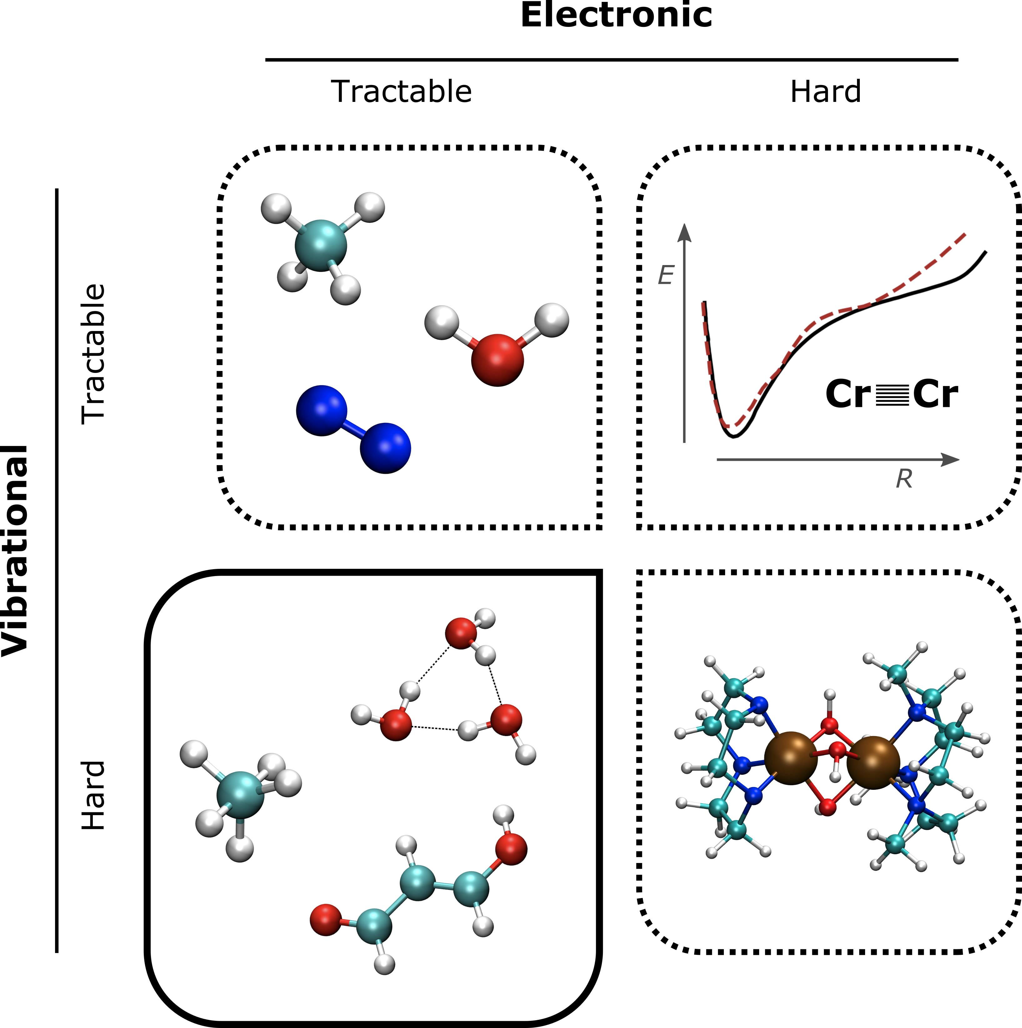
Figure 1: We categorize molecular simulation into four quadrants, depending on whether the electronic structure and vibrational structure of the problem are tractable on a classical computer. This work’s focus is the lower-left quadrant—those molecules or complexes for which the potential energy surface can be calculated on a modern classical computer, while the quantum vibrational structure may require a quantum computer. Upper-left: small rigid molecules methane, water, and nitrogen. Upper-right: the chromium dimer, for which state-of-the-art electronic structure methods (dashed) cannot match experiment (solid)  (?). Lower-right: A chromium-containing large molecule with non-rigid ligands. Lower-left: the prototypical “fluxional” molecule CH${}_{5}^{+}$, the water trimer which contains non-bonded interactions, and malondialdehyde which contains migratory hydrogen atoms.

Even qualitatively correct vibrational spectra often require a rigorous quantum treatment because Fermi resonances, association bands, and other resonance effects can result from small coupling terms  (?, ?, ?, ?). The ability to calculate vibrational structure has many applications including fuel combustion  (?), atmospheric science  (?), astrochemistry  (?, ?), and fundamental experiments in chemical physics  (?, ?). Other than vibrational spectra, problems that lie in the lower-left quadrant of Figure 1 include low-temperature thermodynamic calculations of some bulk solids  (?) and quantum liquids  (?).

Previous quantum computational studies in this area include analog quantum algorithms for quantum vibrations  (?, ?, ?, ?, ?), digital quantum algorithms for finding vibrational states and/or overlaps  (?, ?, ?), and approaches for which vibrational degrees of freedom are coupled to other systems  (?, ?, ?, ?). The present work is distinct in several ways as outlined below.

In this work we present algorithms for calculating vibrational spectra on both near- and long-term hardware, focusing on vibrational infrared spectra. One of our contributions is identifying certain essential components that are required for this problem class, drawing attention to the algorithmic objectives that would not appear in most problems that involve Hamiltonian simulation. Some aims of this class of problems are significantly different from the electronic structure problem, which we introduce to the reader and demonstrate how to overcome. Finally and most importantly, we compare the problem’s complexity characteristics to the electronic structure problem. The results suggest that, for a given precision, a vibrational structure problem instance will probably achieve quantum advantage before an electronic one.

From a Hamiltonian simulation perspective, we note three conceptual differences between the nature of the typical electronic structure problem instance and that of vibrational spectroscopy, the first two of which to our knowledge have not been identified previously in this context. First, when it is said that the “spectrum” is being calculated in molecular electronic structure, this normally refers to at most a handful of the lowest-lying electronic states. In contrast, in a vibrational problem one is almost always interested in many states, which may indeed be far from the ground state (excited states greater than 100 are often of interest).

The second conceptual difference is that one is often interested in calculating both vibrational energies and transition intensities, which necessitates calculating the transition amplitudes with respect to a non-unitary coordinate-dependent operator. Though such transition amplitudes are applicable to electronic structure in some important areas  (?, ?), their inclusion has not been the norm in the context of quantum algorithms. Third, the problem requires that bosons (vibrations) instead of fermions be encoded into the quantum device, a topic that has been previously explored  (?, ?, ?, ?).

2 Theory

In arbitrary internal coordinates $\vec{s}$ (with corresponding momenta $\vec{m}$), the Hamiltonian for $M$ vibrations in general form is written (with $\hbar=1$)

$$H=\frac{1}{2}\sum g_{ij}m_{i}m_{j}+V(\vec{s}).$$ (1)

where $g_{ij}$ is the coupling between momenta (vanishing for $i\neq j$ under normal or Cartesian coordinates) and $V(\vec{s})$ is the potential energy term. In the harmonic approximation, one may diagonalize the Hessian matrix at the equilibrium position, leading to a simplified approximate expression with uncoupled coordinates,

$$H_{\textrm{harm}}=\frac{1}{2}\sum_{i}^{M}\omega_{i}(q_{i}^{2}+p_{i}^{2}),$$ (2)

where $i$ denotes the vibrational mode, $M$ is the total number of modes, $q$ and $p$ are respectively the bosonic position and momentum operators, and $\omega_{i}$ is the energy of mode $i$. It is trivial to find eigenvalue-eigenfunction pairs for equation (2) on a classical computer, since excited states in the Harmonic approximation are product states of separate modes.

Expression (2) can be systematically improved by including higher order anharmonic terms,

$$H_{\textrm{anharm}}=\frac{1}{2}\sum_{i}^{M}\omega_{i}(q_{i}^{2}+p_{i}^{2})+\sum_{\{ijk\}}h_{ijk}q_{i}q_{j}q_{k}+\sum_{\{ijkl\}}h_{ijkl}q_{i}q_{j}q_{k}q_{l}+\cdots,$$ (3)

where the index ordering is irrelevant and $h_{ijk\cdots}=0$ if all indices are distinct. Computational difficulties arise when these higher-order terms are included, due to both the deviation from harmonicity and the coupling between modes.

Even for a molecule of 5 to 8 atoms, the complete inclusion of anharmonic effects can be computationally prohibitive. Though various forms of perturbation theory and dimensionality reduction sometimes yield good results, one must often resort to exact diagonalization of the whole Hilbert space or similarly expensive methods  (?, ?, ?, ?, ?, ?). We note that we are not constrained to use equation (3) but may choose any convenient coordinate system—it will often be the case that choosing a specialized coordinate system allows one to use a lower-order series expansion  (?, ?, ?).

In order to make our discussion concrete, we consider infrared spectroscopy, though similar mathematical methods would be used for other experiments such as Raman, microwave, or ultrafast multidimensional vibrational spectroscopy  (?, ?).

The dipole moment operator is necessary for simulation of light-matter interaction, e.g. for calculating transition intensities. It is denoted $\mu^{(\alpha)}$ where $\alpha\in\{x,y,z\}$ is a Cartesian direction. As $\mu^{(\alpha)}$ is coordinate-dependent, it is associated with a dipole moment surface (DMS), which may be expanded in a power series,

$$\begin{split}\mu^{(\alpha)}&=\mu^{(\alpha)}_{0}+\sum_{i}^{M}\left.\frac{\partial\mu^{(\alpha)}}{q_{i}}\right|_{q_{i}=0}q_{i}+\frac{1}{2}\sum_{ij}^{M}\left.\frac{\partial^{2}\mu^{(\alpha)}}{q_{i}q_{j}}\right|_{q_{i},q_{j}=0}q_{i}q_{j}+\cdots\\ &=\mu^{(\alpha)}_{0}+\sum_{i}^{M}m_{i}q_{i}+\sum_{ij}^{M}m_{ij}q_{i}q_{j}+\cdots\end{split}$$ (4)

The objective is to calculate

$$f(\omega)=\sum_{\alpha}\sum_{j}|\langle 0|\mu^{(\alpha)}|j\rangle|^{2}\mathcal{L}(\omega_{j}-\omega)$$ (5)

where $|0\rangle$ is the initial eigenstate (ground state when beginning from zero temperature), $\mu^{(\alpha)}$ is the dipole operator for Cartesian direction $\alpha$, and $\mathcal{L}(\omega)$ is a line shape function, approximated as a delta function when one does not consider broadening effects. Though in this work we consider transitions from the ground state, the initial state of interest is often a Gibbs state (i.e. thermal state). Existing quantum algorithms for thermal state preparation  (?, ?, ?, ?, ?) may be used in conjunction with the approaches summarized here. Note that expression (5) is mathematically similar to what is used to calculate Franck-Condon factors  (?, ?), where $\mu^{(\alpha)}=I$ and a different Hamiltonian is used.

Both the Hamiltonian and the dipole operator may be mapped to a qubit-based Hamiltonian using the bosonic commutation relations, where a practical choice is to use the Pauli operator basis:

$$H_{\textrm{anharm}}\mapsto\sum_{k}^{N_{P}}a_{k}P_{k}=\sum_{k}a_{k}\bigotimes_{g}^{N_{q}}\sigma_{gk},$$ (6)

$$\mu^{(\alpha)}\mapsto\sum_{k}^{N_{R}^{(\alpha)}}b_{k\alpha}R_{k\alpha}=\sum_{k}b_{k\alpha}\bigotimes_{g}^{N_{q}}\sigma_{gk\alpha},$$ (7)

where $g$ labels the qubit, $\sigma_{g}\in\{I,X,Y,Z\}$ is the identity or a Pauli operator, $N_{P}$ ($N_{R}^{(\alpha)}$) is the number of Pauli strings in the encoded operator, and $N_{q}$ is the number of qubits. Several encodings for performing this mapping have been discussed previously  (?, ?, ?, ?), with evidence that the Gray code offers reasonable resource trade-offs  (?).

A near-term algorithm for the vibrational spectroscopy problem requires several elements: (a) mapping of bosons to qubits, (b) finding unitaries $U_{i}$ to produce eigenstates, (c) determining state overlaps $|\langle\psi_{i}|\psi_{j}\rangle|^{2}$, (d) calculating transition amplitudes with respect to a non-unitary Hermitian operator, and (e) efficiently finding eigenstates far above the ground state. We first present the noisy intermediate-scale quantum (NISQ) approach for these problem requirements, before briefly summarizing a long-term approach that addresses all algorithmic requirements.

2.1 Near-term algorithms.

Using near-term quantum hardware, ground and excited states may be found using previously published variational methods  (?, ?, ?, ?, ?, ?). For a given vibrational eigenstate $|\psi_{j}\rangle$, a variational method used with a classical optimizer will lead to a circuit unitary $U_{j}$ yielding $U_{j}|0\rangle=|\psi_{j}\rangle$. Additionally, expression (5) requires a method for calculating state overlaps $|\langle\psi_{i}|\psi_{j}\rangle|^{2}$, for which quantum subroutines are summarized in the Supplementary Information (SI).

In order to calculate arbitrary transition amplitudes $|\langle\psi_{i}|A|\psi_{j}\rangle|^{2}$ on near-term hardware, a naive approach would require an efficient method for considering cross-terms such as $\langle\psi_{i}|0\rangle$ or $\langle\psi_{i}|(\Pi_{k}\sigma_{k})|0\rangle$ (where $(\Pi_{k}\sigma_{k})$ is a Pauli string), in addition to their absolute values squared. This is a nontrivial task, since quantum computers naturally output overlaps squared. Though inner products may be calculated with so-called Hadamard tests that require a substantially increased circuit depth if only one- and two-qubit gates are allowed  (?), a much shorter-depth method was recently found  (?) for calculating transition amplitudes of arbitrary operators.

Tailoring the latter work to vibrational spectroscopy, the procedure is to use an additional set of unitaries,

$$V_{kl,\pm}^{(\alpha)}=\frac{1}{2}(I\pm R_{k\alpha})(I\pm R_{l\alpha})=e^{\pm R_{k\alpha}\pi/4}e^{\pm R_{l\alpha}\pi/4}$$ (8)

for all $l,k<N_{R}^{(\alpha)}$. One then proceeds to reproduce $|\langle i|\mu^{(\alpha)}|j\rangle|^{2}$ from many measurements on the circuit set $U_{i}^{\dagger}V_{kl,\pm}U_{j}|0\rangle$ (see SI). Thus one increases the depth of two state preparation circuits by a small constant factor and collects measurement statistics from a quadratic (in $N_{p}$) number of circuits. This procedure is performed for every eigenenergy for which one wishes to calculate the transition amplitude. The algorithm requires a larger total number of measurements, but the fact that it increases circuit depth by only a small factor makes it ideal for near-term hardware.

2.2 Spectral window focusing.

Not only are we often interested in many vibrational eigenstates—it is also often the case that one is concerned only with high-lying excited states (for instance the 100th excited state and above). This may be the case when: part of a spectrum is blocked by background noise; an astronomical telescope is able to read only part of the infrared spectrum; or only a specific band is technologically relevant. Additionally, different regions of the spectrum contain different information. For example, in water clusters relevant to atmospheric chemistry, the OH stretches (3800 to 3000 cm^-1) report on local environments while the low-frequency region reports on collective motion  (?). Therefore it may be a waste of computational effort to find eigenstates outside the energy window of interest.

We point this out because it means the goal of the vibrational spectrum problem often differs from other Hamiltonian simulation problems, leading to important considerations in algorithm design that have not been widely investigated.

The notable consequence is that most hereto proposed near-term algorithms for excited states are not always viable. This is because in their canonical forms, most existing near-term approaches  (?, ?, ?, ?, ?, ?) require one to find the low-energy eigenvector subspace as a way to build up to the desired excited state. In other words, if one is not interested in the first $W$ excited states, then the larger $W$ is the more one would like to largely avoid the costly determination of the subspace spanned by $\{\psi_{1},\psi_{2},\cdots,\psi_{W}\}$, where $\psi_{m}$ is the mth excited state.

We highlight one possible (previously proposed) near-term algorithmic solution for determining high-lying excited states, that may be used in conjunction with the previously mentioned methods. This is to use the folded spectrum method  (?, ?), which easily allows one to select an energy neighborhood. The folded Hamiltonian is defined as

$$H_{fold}=(H-\zeta I)^{2}$$ (9)

where $\zeta$ is an arbitrary constant. The lowest eigenstates of $H_{fold}$ are those eigenstates of $H$ which are closest in energy to $\zeta$. This approach quadratically increases the number of Pauli terms in the effective Hamiltonian, allowing one to “zoom in” on an arbitrary portion of the spectrum. We do not rule out more efficient methods for high-lying excited states.

2.3 Utility of incomplete spectra.

When using variational algorithms and NISQ hardware to determine portions of the spectra, one may be able to calculate only incomplete spectra. This is due to the nature of many hybrid quantum-classical algorithms; it is usually not possible to guarantee that all eigenstates in a given energy region have been found. Hence it is important to note that even a spectrum with missing peaks is often useful. First, one may be interested in only a few specific spectral features in the region, in which case one may focus efforts converging to those specific transitions. Second, and perhaps more importantly, the goal is often to determine whether a candidate molecule matches an experimental result. If some spectral features in the computed spectrum of the candidate molecule are not present in the experimental spectrum, then the candidate molecule may be removed from consideration.

2.4 Long-term hardware.

A long-term fully error-corrected solution to these problems is to use quantum phase estimation (QPE)  (?) to produce a probabilistic set of measurements. This approach has been discussed previously  (?, ?, ?), first by Wecker and co-workers  (?). In the more typical use of QPE, one first attempts to prepare a state with as much overlap as possible with a particular eigenstate, e.g. the ground state. In the context of the this work, QPE is instead used in a way that allows one to calculate a full response spectrum  (?, ?, ?), i.e. determining the non-negligible values $|\langle\eta_{0}|\hat{A}|\psi_{i}\rangle|^{2}$, where $\hat{A}|\eta_{0}\rangle$ is not necessarily an eigenstate of the Hamiltonian but the $\{|\psi_{i}\rangle\}$ are eigenstates. First consider the case of $\hat{A}=\hat{I}$. One runs the same QPE algorithm, but sets the initial state to $|\eta_{0}\rangle$, which is in general not an eigenstate, such that $|\eta_{0}\rangle=\sum_{i}c_{i}|\psi_{i}\rangle$. After running QPE, one is left with a superposition of eigenstate-eigenphase pairs, as shown in the expression

$$\sum c_{i}|\psi_{i}\rangle|0\rangle\xrightarrow{\textrm{QPE}}\sum c_{i}|\psi_{i}\rangle|\tilde{\phi}_{i}\rangle.$$ (10)

In contrast to the standard use of QPE, in this case we are interested in more than just one eigenstate. The algorithm proceeds as follows. One performs many repetitions of the circuit, measuring register $E$ after each run, yielding a phase $\tilde{\phi}_{i}$. From many measurements one then composes a histogram where each bin is an $N_{E}$-bit value $\tilde{\phi}_{i}$. This histogram is the desired response spectrum with resolution determined by $N_{E}$, and the process terminates once the histogram has converged.

One advantage of this method is that it effectively combines many eigenstates into a single measurement. This is especially useful for vibrational spectra, where one is often interested in more than just a few eigenstates of the spectrum. For a particular $N_{E}$, there is a subset of eigenstates $\mathcal{D}_{j}$ $=\{\psi_{j1},\psi_{j2}\cdots\}$ all of which yield $\tilde{\phi}_{j}$. Hence if the measurement yields $\tilde{\phi}_{j}$, this means register $S$ has collapsed to the superposition $\mathcal{N}\sum_{k\in\mathcal{D}_{j}}c_{k}|\psi_{k}\rangle$, where $\mathcal{N}$ is a normalization constant. The beneficial result is that the probabilities of many nearby eigenenergies are combined, and the number of required measurements is dependent on $N_{E}$ but independent of the size of the problem Hamiltonian.

As discussed, vibrational (e.g. infrared) spectroscopy requires calculating the action of an arbitrary non-unitary operator $\mu^{(\alpha)}$ on a prepared state. Roggero et al.  (?) solved the problem of linear response with respect to a non-unitary operator. After adding one ancilla qubit, one may apply the operator

$$U_{\mu,\alpha,\gamma}=\begin{pmatrix}\cos\gamma\mu^{(\alpha)}&-\sin\gamma\mu^{(\alpha)}\\ \sin\gamma\mu^{(\alpha)}&\cos\gamma\mu^{(\alpha)}\\ \end{pmatrix}$$ (11)

to an arbitrary state $|\psi\rangle$, which will yield $\mathcal{N}\mu^{(\alpha)}|\psi\rangle$ with probability $P_{success}=\langle\psi|\sin(\gamma\mu^{(\alpha)})|\psi\rangle$, where $\mathcal{N}=||\mu^{(\alpha)}|\psi\rangle||^{-1}$ is a normalization constant. This unitary probabilistically produces the desired state $|\Phi_{0}^{(\alpha)}\rangle\equiv$ $\hat{\mu}^{(\alpha)}|\eta_{0}\rangle/\lVert\hat{\mu}^{(\alpha)}|\eta_{0}\rangle\rVert$. If the ancilla is measured to be $|0\rangle$ ($|1\rangle$) then the state preparation has succeeded (failed). The remainder of the algorithm then proceeds as in the $\hat{A}=\hat{I}$ case, with $|\eta_{0}\rangle$ replaced by $|\Phi_{0}^{(\alpha)}\rangle$.

Finally, we posit that there are promising strategies for “spectral window focusing” in long-term hardware as well. For the QPE-based method, the goal would be to make the histogram measurements fall primarily within a particular energy window, as measurements outside the window are not of interest. In principle one may use amplitude amplification methods  (?, ?) to boost the probability of the desired eigenenergy window. The result is that fewer measurements would be required to produce the histogram in the energy window of interest, at the cost of an increase in circuit depth. We leave a full description to future work.

3 Comparison to electronic structure

The first physics simulation to achieve quantum advantage is likely to be a nearest-neighbor toy model such as an Ising model  (?), because only $\mathcal{O}(N)$ two-body interactions are present. But it is important to consider what will be the first real-world non-toy simulation to show quantum advantage. Here we argue that, to a given energy precision, the first such simulation of a molecule is more likely to be a vibrational problem instance than an electronic one. Note that the electronic structure Hamiltonian may be written as

$$H_{\textrm{ES}}=\sum h_{ij}a_{i}^{\dagger}a_{j}+\sum h_{ijkl}a_{i}^{\dagger}a_{j}^{\dagger}a_{k}a_{l},$$ (12)

where $a_{i}^{\dagger}$ and $a_{i}$ are fermionic creation/annihilation operators for the $i$th orbital and coefficients $h_{ij}$ and $h_{ijkl}$ are determined by calculating overlap integrals. 2- and 4-body terms are present, and in real molecules one effectively sees nearly all-to-all connectivity between the electronic orbitals. For simplicity we write equation (12) without spin constraints (see SI), though our results do account for spin degrees of freedom.

The quantum resources required for the vibrational problem depend on the order of the expansion needed for sufficient precision in equation (3). We observe that early molecular targets for quantum computing ought to be those for which (a) classical computational approaches (e.g. perturbation theory) fail and (b) the highest relevant order is 4 or less. Both requirements are likely to hold for a substantial set of molecules  (?, ?).

A third-order Hamiltonian has four types of terms: $p_{i}^{2}$, $q_{i}^{2}$, $q_{i}^{3}$, $q_{i}^{2}q_{j}$. A fourth-order Hamiltonian has 8 types with the inclusion of $q_{i}^{4}$, $q_{i}^{3}q_{j}$, $q_{i}^{2}q_{j}^{2}$, and $q_{i}^{2}q_{j}q_{k}$. In the SI we give Pauli operator counts for each of these 8 term types, for $d=4$ (2 qubits) and $d=8$ (3 qubits).

A key insight is that fourth-order vibrational Hamiltonians scale at most as $\mathcal{O}(M^{3})$ in the number of modes $M$. However, depending on the choice of coordinate system  (?, ?, ?, ?) it is often possible to exclude three-body interactions, leading to a scaling of $\mathcal{O}(M^{2})$ terms. This scaling is more favorable than molecular electronic structure, for which near-term implementations would require approximately $\mathcal{O}(N^{4})$ Hamiltonian terms in the number of orbitals $N$. Notably, it is more common to see sparser interactions in vibrational problems than in electronic structure problems, because it is often the case that some vibrational modes show negligible coupling to the other modes—this implies $\mathcal{O}(M^{2})$ may often be an overestimate.

Our case hinges on the notion that a Hamiltonian with more terms and with higher Pauli lengths is likely to require more resources to simulate, regardless of whether one is using near- or long-term hardware. The asymptotic scaling on its own does not prove the argument though. One must still investigate (a) whether the pre-factor to the vibrational Hamiltonians’ term count is sufficiently small for lower qubit counts, (b) the distributions of lengths of the Pauli strings, and (c) Hamiltonian magnitudes, all of which we study below.

Notably, there has been extensive recent progress in reducing the asymptotic scaling of quantum algorithms for electronic structure  (?, ?, ?, ?). However, due to these newer algorithms’ need for a larger basis set and/or an increase in the number of required qubits, these methods are not amenable to accurate molecular simulation for qubit counts below 100  (?). Even if one assumes that error-corrected hardware is required for solving any instance of both the vibrational and electronic problems, it remains likely that the subset of vibrational problems with $\mathcal{O}(M^{2})$ or $\mathcal{O}(M^{3})$ Pauli terms will be solvable before any electronic structure instance, based on our analysis. Caveats and important further justification of our methods of comparison can be found in the SI.

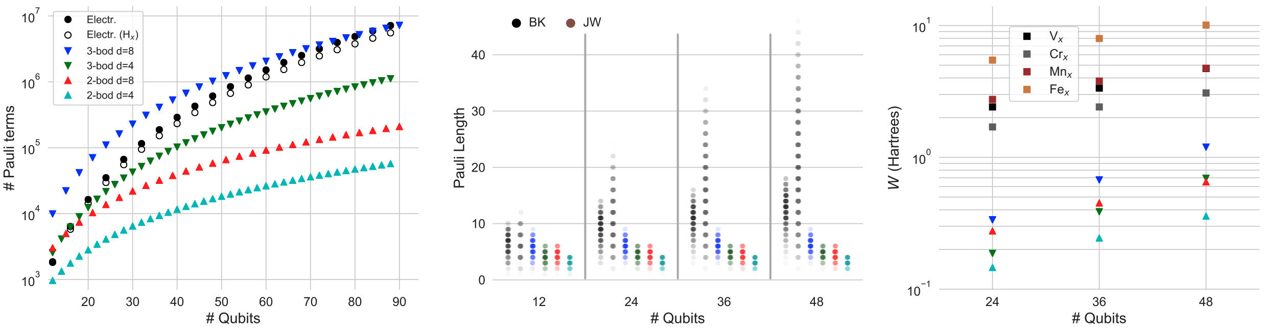
Figure 2: Left: Number of Pauli strings in the qubit Hamiltonian versus the number of qubits, for the standard electronic structure problem and some classes of vibrational structure. Filled circles represent analytical results and unfilled circles represent numerical results from a collection of hydrogen atoms. Triangles represent analytical results for fourth-order vibrational Hamiltonians, where e.g. 3-bod $d$=8 signifies a truncation of 8 vibrational levels where at most three-body terms are included. Center: Probability distributions of Pauli lengths in six Hamiltonian classes. BK and JW respectively denote the Bravyi-Kitaev and Jordan-Wigner mappings for the electronic structure problem. Right: The magnitude $W$, which is related to the Frobenius matrix norm, for various Hamiltonians. $W$ should be compared only between Hamiltonians of the same size. The squares signify model electronic structure Hamiltonians of V_x, Cr_x, Mn_x, and Fe_x, for $x\in\{2,3,4\}$. Pessimistically large couplings are used for the vibrational Hamiltonians (see SI). All vibrational results use fourth-order Hamiltonians.

4 Results

Proxies for quantum resource comparisons. All our vibrational data is for fourth-order Hamiltonians, where we use bosonic truncations $d=$ 4 or 8 and have considered both the exclusion and inclusion of 3-body terms $q_{i}^{2}q_{j}q_{k}$. Though the electronic structure problem scales as $\mathcal{O}(N^{4})$ against the $\mathcal{O}(M^{3})$ or $\mathcal{O}(M^{2})$ vibrational scaling of some molecules, the latter always have a larger constant factor (left, Figure 2). However, for the majority of cases considered here, these results show that the electronic structure Hamiltonians contain more terms for qubit counts great than $\sim$20.

For simplicity, we consider only cases in which all modes have equal $d$. In reality, each mode would require a different truncation, meaning that the number of Pauli strings would lie in between the plotted trends. For the electronic problem instances, the analytical results (filled circles) are comparable to the numerical results (open circles) obtained from 3D arrays of hydrogen atoms (see SI). Note that the number of Pauli terms is equal for the Jordan-Wigner (JW)  (?) and Bravyi-Kitaev (BK)  (?) encodings, though their length distributions are unequal.

The center panel of Figure 2 shows the distribution of Pauli lengths, another important indicator of a problem Hamiltonian’s complexity. For the subset of vibrational problem instances considered (fourth-order Hamiltonians with truncations of $d\leq 8$), vibrational problems are more local than electronic problems, even for low qubit counts and when compared against the logarithmically scaling BK mapping.

Another factor determining simulation complexity is the magnitude of the Hamiltonian. There are different matrix norms used in quantum algorithm analysis, and resource bounds are usually derived in terms of both a norm and the desired precision, among other considerations  (?, ?, ?, ?, ?). In addition, the number of measurements for VQE depends on the magnitude of the terms  (?, ?), which is closely related to our expression below. For a simple and easily computed comparison of Hamiltonian magnitudes, we use the quantity

$$W=\sqrt{\sum_{k\neq I}a_{k}^{2}},$$ (13)

where $k\neq I$ signifies that the coefficient preceding the identity operator is excluded. Notably, $W2^{N_{q}/2}$ is an upper bound to the Frobenius norm. $W$ should be used for comparisons only between Hamiltonians on the same number of qubits.

We constructed minimal-basis electronic structure model Hamiltonians for transition metals V_x, Cr_x, Mn_x, and Fe_x, where $x=$ 2, 3, and 4 correspond to 24, 36, and 48 qubits, respectively (see SI). These were meant to provide typical order-of-magnitude matrices for transition metal elements. We constructed vibrational Hamiltonians with deliberately pessimistic couplings. Harmonic values were evenly spaced between 1000 and 4000 cm^-1, every third-order vibrational term was set to 400 cm^-1, and every fourth-order term was set to 40 cm^-1.

Despite the pessimistically complex vibrational Hamiltonians, $W$ values for the two-body Hamiltonian are close to an order of magnitude smaller than the four types of electronic model Hamiltonians, while $W$ for the three-body vibrational Hamiltonians remain several times smaller (right panel of Figure 2).

Additionally, the lower locality of the vibrational Hamiltonians imply that $W$, if used as an approximate proxy for simulation complexity, further underestimates the difference between vibrational and electronic problems. This is because some long-term Hamiltonian algorithms  (?) scale with locality (center panel of Figure 2), and near-term VQE requires fewer measurements with a more local Hamiltonian  (?, ?).

We note again that the required quantum resources are precision dependent. For both vibrational and electronic problems, different applications have wildly different precision requirements. A reasonable candidate for the first practical vibrational problem is the calculation of zero-point energy or low-lying transitions in a vibrational problem to sub-chemical precision. See the SI for further discussion.

Detailed resource estimates are beyond the scope of this work, but these order-of-magnitude differences between vibrational and electronic Hamiltonians are noteworthy. These three metrics (term counts, locality, and $W$) seem to support the postulate that a vibrational problem instance may achieve quantum advantage before an electronic problem instance.

IR spectra. As a proof of concept, we performed numerical simulations and error analyses on four vibrational Hamiltonians: carbon monoxide (CO), the isoformyl radical (COH), ozone (O₃), and a model Hamiltonian of Fermi resonance (Figure 3).

We studied Trotter error for both the approximate unitary used in QPE and the approximate imaginary time evolution (ITE) operator appropriate for some nearer-term algorithms. For the former case, we constructed the unitary matrix

$$\tilde{U}(\Delta\tau)=\prod_{k}^{N_{P}}e^{-i\Delta\tau a_{k}P_{k}}.$$ (14)

where $\Delta\tau$ is the time step. This is a first-order Trotter approximation to the quantum propagator $U(\Delta\tau)\equiv\exp(-i\Delta\tau H)$. We then diagonalized $\tilde{U}(\Delta\tau)$ and compared the ordered eigenvalues to the exact result.

In our simulation of ITE, we instead constructed the operator

$$\tilde{M}(\Delta\beta)=\prod_{k}^{N_{P}}e^{-\Delta\beta a_{k}P_{k}}$$ (15)

where $\Delta\beta$ is an ITE step. For all but the ground state, formula (15) used the Pauli representation of the folded Hamiltonian, not of the original Hamiltonian. Folded Hamiltonians were used in order to highlight the use of a method that allows one to skip irrelevant eigenstates, effectively implementing spectral window focusing. Calculations were implemented using SciPy  (?).

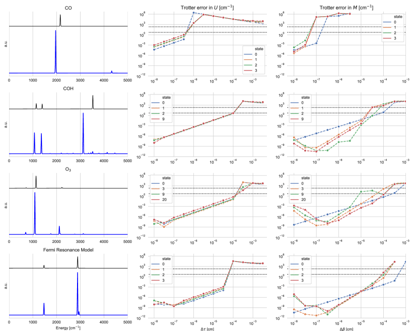
Figure 3: Vibrational infrared spectra for carbon monoxide (CO), the isoformyl radical (COH), ozone (O₃), and a Fermi resonsance model Hamiltonian. The first column shows the infrared spectra (blue) and their harmonic approximation (black) in arbitrary units, summing intensities in all Cartesian directions. Peaks were broadened with Gaussians of arbitrary standard deviation 10 cm^-1. The second column shows Trotterization error in the quantum time propagator, which is relevant to long-term algorithms. The third column shows Trotterization error in the imaginary time evolution operator, relevant to some NISQ approaches. Excited states in the third column are found using the folded Hamiltonian method. Horizontal dotted lines are drawn at 5 cm^-1, an arbitrary high-accuracy threshold required for many spectroscopy applications; and at 209 cm^-1, equal to $k_{B}T$ at room temperature and approximately half of chemical accuracy.

Figure 3 shows the infrared spectra (blue). The harmonic approximations (black) are plotted; the contrast between the two plots demonstrates the importance of including higher-order anharmonic terms that are hard to simulate classically. Qualitative differences such as the the extra peaks that appear (e.g. at 2940 cm^-1 in the Fermi resonance Hamiltonian) tend to be difficult to obtain classically, often failing under perturbation theory  (?, ?).

The second column shows the Trotterization error in some of the more intense transitions’ eigenvalues against increasing $\Delta\tau$. These are related to long-term algorithms, both in running QPE and in dynamical simulations. The third column approximates the ITE operator’s error by Trotterization with finite length $\Delta\beta$. These are more relevant to noisy intermediate-scale quantum (NISQ) algorithms, both for ITE  (?) and variational anstazae based on ITE  (?).

Errors in $U$ are mostly independent of the eigenstates, while errors in $M$ are distributed over many orders of magnitude even for fixed $\Delta\beta$. This may be partly because each folded Hamiltonian is in fact a different Hamiltonian. Notably, all non-monotonic behavior in the ITE error plots arise only in folded Hamiltonians—the cause of this behavior is intriguing but unclear. CO requires the smallest (i.e. worst) time step, which we hypothesize might be due to the lack of favorable error cancellation, as cancellation may be more prominent in Hamiltonians with more terms. There was no clear trend with respect to the (Froebenius) norms of the Hamiltonians (data not shown), though in the worse case (carbon monoxide) the error becomes unacceptably large approximately when $\Delta\tau$ and $\Delta\beta$ have order of magnitude comparable to the inverse norm of the Hamiltonian ($1/\|H\|$). The resulting error trends give an indication of the step sizes needed for accurate simulation of small molecules, though further study is needed to determine broadly applicable relationships between vibrational problem instances and Trotter error.

5 Outlook

Although molecular electronic structure is often the first candidate offered for near-term quantum simulation of a real-world substance, we have provided evidence suggesting that molecular vibrational structure will likely, for a given energy precision, achieve quantum advantage first. After considering previously unidentified requirements in designing quantum algorithms for vibrational spectra, we have presented approaches for solving this class of problems on both near-term and long-term quantum computers, addressing the components that make this mathematically distinct from the electronic structure problem: calculating transition amplitudes with respect to a non-unitary operator and calculating high-lying excited states. Future research should focus on more detailed resource counts including estimates of circuit depth and gate complexity, as well as inclusion of rotational and other degrees of freedom. This work advances the applicability of quantum computation for atmospheric science, many biomolecular interactions, fuel combustion, gas-phase reactions, and astrochemistry, while implying that some focus for near-term quantum applications ought to shift to scientifically relevant vibrational problems.

Supplementary Information

Additional details regarding mapping vibrational modes to qubits, near-term quantum algorithms for finding spectra, the complexity comparison between vibrational and electronic problem classes, counting terms for fermionic and bosonic operators, and calculation of potential energy and dipole surfaces.

References

- 1. S. McArdle, S. Endo, A. Aspuru-Guzik, S. C. Benjamin, X. Yuan, Rev. Mod. Phys. 92, 015003 (2020).
- 2. Y. Cao, et al., Chem. Rev. 119, 10856 (2019).
- 3. S. McArdle, A. Mayorov, X. Shan, S. Benjamin, X. Yuan, Chem. Sci. 10, 5725 (2019).
- 4. P. F. Bernath, Spectra of Atoms and Molecules (Second Edition) (Oxford University Press, New York, 2005).
- 5. S. Mukamel, Principles of Nonlinear Optical Spectroscopy (Oxford University Press, 1999).
- 6. E. B. Wilson, J. C. Decius, P. C. Cross, Molecular Vibrations: The Theory of Infrared and Raman Vibrational Spectra (Dover Publications, Mineola, NY, USA, 1980).
- 7. P. Jankowski, A. R. W. McKellar, K. Szalewicz, Science 336, 1147 (2012).
- 8. S. E. Brown, et al., J. Am. Chem. Soc. 139, 7082 (2017).
- 9. N. Yang, C. H. Duong, P. J. Kelleher, A. B. McCoy, M. A. Johnson, Science 364, 275 (2019).
- 10. M. Riera, S. E. Brown, F. Paesani, J. Phys. Chem. A 122, 5811 (2018).
- 11. P. Bajaj, J. O. Richardson, F. Paesani, Nat. Chem. 11, 367 (2019).
- 12. S. Guo, M. A. Watson, W. Hu, Q. Sun, G. K.-L. Chan, J. Chem. Theory Comput. 12, 1583 (2016).
- 13. J. Vázquez, J. F. Stanton, Mol. Phys. 105, 101 (2007).
- 14. E. L. Sibert, D. P. Tabor, N. M. Kidwell, J. C. Dean, T. S. Zwier, J. Phys. Chem. A 118, 11272 (2014).
- 15. A. B. McCoy, T. L. Guasco, C. M. Leavitt, S. G. Olesen, M. A. Johnson, Phys. Chem. Chem. Phys. 14, 7205 (2012).
- 16. L. B. Harding, Y. Georgievskii, S. J. Klippenstein, J. Phys. Chem. A 121, 4334 (2017).
- 17. G.-L. Hou, et al., J. Phys. Chem. Lett. 4, 779 (2013).
- 18. V. Barone, M. Biczysko, C. Puzzarini, Acc. Chem. Res. 48, 1413 (2015).
- 19. B. A. McGuire, et al., Science 359, 202 (2018).
- 20. S. Ospelkaus, et al., Phys. Rev. Lett. 104, 030402 (2010).
- 21. R. F. Ribeiro, L. A. Martinez-Martinez, M. Du, J. Campos-Gonzalez-Angulo, J. Yuen-Zhou, Chem. Sci. 9, 6325 (2018).
- 22. V. Kapil, E. Engel, M. Rossi, M. Ceriotti, J. Chem. Theory Comput. 15, 5845 (2019).
- 23. A. J. Leggett, Quantum Liquids: Bose Condensation and Cooper Pairing in Condensed-Matter Systems (Oxford University Press, 2006), first edn.
- 24. J. Huh, G. G. Guerreschi, B. Peropadre, J. R. Mcclean, A. Aspuru-Guzik, Nat. Photonics 9, 615 (2015).
- 25. C. Sparrow, et al., Nature 557, 660 (2018).
- 26. S. Joshi, A. Shukla, H. Katiyar, A. Hazra, T. S. Mahesh, Phys. Rev. A 90, 022303 (2014).
- 27. A. Teplukhin, B. K. Kendrick, D. Babikov, J. Chem. Theory Comput. 15, 4555 (2019).
- 28. R. J. MacDonell, et al., arXiv (2020). arXiv:2012.01852.
- 29. N. P. D. Sawaya, J. Huh, J. Phys. Chem. Lett. 10, 3586 (2019).
- 30. P. J. Ollitrault, A. Baiardi, M. Reiher, I. Tavernelli, Chem. Sci. 11, 6842 (2020).
- 31. L. Veis, J. Višňák, H. Nishizawa, H. Nakai, J. Pittner, Int. J. Quantum Chem. 116, 1328 (2016).
- 32. A. Macridin, P. Spentzouris, J. Amundson, R. Harnik, Phys. Rev. Lett. 121, 110504 (2018).
- 33. A. B. Magann, M. D. Grace, H. A. Rabitz, M. Sarovar, arXiv (2020). arXiv:2002.12497.
- 34. P. J. Ollitrault, G. Mazzola, I. Tavernelli, arXiv (2020). arXiv:2006.09405.
- 35. T. Kosugi, Y.-i. Matsushita, Phys. Rev. Research 2, 033043 (2020).
- 36. X. Cai, W.-H. Fang, H. Fan, Z. Li, arXiv (2020). arXiv:2001.03406.
- 37. R. Somma, G. Ortiz, E. Knill, J. Gubernatis, arXiv (2003). arXiv:quant-ph/0304063.
- 38. N. P. D. Sawaya, et al., npj Quantum Inf. 6, 49 (2020).
- 39. N. P. D. Sawaya, G. G. Guerreschi, A. Holmes, 2020 IEEE International Conference on Quantum Computing and Engineering (QCE) (IEEE, 2020).
- 40. J. M. Bowman, T. Carrington, H.-D. Meyer, Mol. Phys. 106, 2145 (2008).
- 41. J. C. Light, Z. Bačić, J. Chem. Phys. 87, 4008 (1987).
- 42. E. L. Sibert, J. Chem. Phys. 88, 4378 (1988).
- 43. X.-G. Wang, T. Carrington, J. Chem. Phys. 129, 234102 (2008).
- 44. A. van der Avoird, D. J. Nesbitt, J. Chem. Phys. 134, 044314 (2011).
- 45. Z. Lin, A. B. McCoy, J. Phys. Chem. A 119, 12109 (2015).
- 46. G. Simons, R. G. Parr, J. M. Finlan, J. Chem. Phys. 59, 3229 (1973).
- 47. J. Zúñiga, J. A. G. Picón, A. Bastida, A. Requena, J. Chem. Phys. 122, 224319 (2005).
- 48. I. W. Bulik, M. J. Frisch, P. H. Vaccaro, J. Chem. Phys. 147, 044110 (2017).
- 49. D. Poulin , P. Wocjan, Phys. Rev. Lett. 103, 220502 (2009).
- 50. A. Riera, C. Gogolin, J. Eisert, Phys. Rev. Lett. 108, 080402 (2012).
- 51. M. Motta, et al., Nat. Phys. 16, 205 (2019).
- 52. A. N. Chowdhury, G. H. Low, N. Wiebe, arXiv (2020). arXiv:2002.00055.
- 53. Y. Wang, G. Li, X. Wang, arXiv (2020). arXiv:2005.08797.
- 54. O. Higgott, D. Wang, S. Brierley, Quantum 3, 156 (2019).
- 55. T. Jones, S. Endo, S. McArdle, X. Yuan, S. C. Benjamin, Phys. Rev. A 99, 062304 (2019).
- 56. J. R. McClean, J. Romero, R. Babbush, A. Aspuru-Guzik, New J. Phys. 18, 023023 (2016).
- 57. L.-W. Wang, A. Zunger, J. Chem. Phys. 100, 2394 (1994).
- 58. P. J. Ollitrault, et al., arXiv (2019). arXiv:1910.12890.
- 59. K. Mitarai, K. Fujii, Phys. Rev. Research 1, 013006 (2019).
- 60. Y. Ibe, et al., arXiv (2020). arXiv:2002.11724.
- 61. F. Perakis, et al., Chem. Rev. 116, 7590 (2016).
- 62. J. R. McClean, M. E. Kimchi-Schwartz, J. Carter, W. A. de Jong, Phys. Rev. A 95, 042308 (2017).
- 63. R. Santagati, et al., Sci. Adv. 4, eaap9646 (2018).
- 64. D. S. Abrams, S. Lloyd, Phys. Rev. Lett. 83, 5162 (1999).
- 65. D. Wecker, et al., Phys. Rev. A 92, 062318 (2015).
- 66. A. Roggero, J. Carlson, Phys. Rev. C 100, 034610 (2019).
- 67. L. K. Grover, Proceedings of the twenty-eighth annual ACM symposium on Theory of computing - STOC 96 (ACM Press, 1996).
- 68. L. K. Grover, Phys. Rev. Lett. 80, 4329 (1998).
- 69. A. M. Childs, D. Maslov, Y. Nam, N. J. Ross, Y. Su, Proc. Natl. Acad. Sci. 115, 9456 (2018).
- 70. R. C. Fortenberry, X. Huang, A. Yachmenev, W. Thiel, T. J. Lee, Chem. Phys. Lett. 574, 1 (2013).
- 71. E. L. Sibert, J. Chem. Phys. 150, 090901 (2019).
- 72. R. Babbush, et al., Phys. Rev. X 8, 011044 (2018).
- 73. R. Babbush, et al., Phys. Rev. X 8, 041015 (2018).
- 74. D. W. Berry, C. Gidney, M. Motta, J. R. McClean, R. Babbush, Quantum 3, 208 (2019).
- 75. V. von Burg, et al., arXiv (2020). arXiv:2007.14460.
- 76. P. Jordan, E. Wigner, Z. Angew. Phys. 47, 631 (1928).
- 77. S. B. Bravyi, A. Y. Kitaev, Ann. Phys. 298, 210 (2002).
- 78. D. W. Berry, A. M. Childs, R. Kothari, 2015 IEEE 56th Annual Symposium on Foundations of Computer Science (2015), pp. 792–809.
- 79. D. W. Berry, A. M. Childs, R. Cleve, R. Kothari, R. D. Somma, Phys. Rev. Lett. 114, 090502 (2015).
- 80. G. H. Low, I. L. Chuang, Phys. Rev. Lett. 118, 010501 (2017).
- 81. A. M. Childs, Y. Su, M. C. Tran, N. Wiebe, S. Zhu, arXiv (2019). arXiv:1912.08854.
- 82. J. F. Gonthier, et al., arXiv (2020). arXiv:2012.04001.
- 83. P. Virtanen, et al., Nat. Methods 17, 261 (2020).
- 84. S. McArdle, et al., npj Quantum Inf. 5, 75 (2019).