Impact of high energy beam tunes on the sensitivities to the standard unknowns at DUNE

Abstract

Even though neutrino oscillations have been conclusively established, there are a few unanswered questions pertaining to leptonic Charge Parity violation (CPV), mass hierarchy (MH) and $\theta_{23}$ octant degeneracy. Addressing these questions is of paramount importance at the current and future neutrino experiments including the Deep Underground Neutrino Experiment (DUNE) which has a baseline of 1300 km. In the standard mode, DUNE is expected to run with a low energy (LE) tuned beam which peaks around the first oscillation maximum ($2-3$ GeV) (and then sharply falls off as we go to higher energies). However, the wide band nature of the beam available at long baseline neutrino facility (LBNF) allows for the flexibility in utilizing beam tunes that are well-suited at higher energies as well. In this work, we utilize a beam that provides high statistics at higher energies which is referred to as the medium energy (ME) beam. This opens up the possibility of exploring not only the usual oscillation channels but also the $\nu_{\mu}\to\nu_{\tau}$ oscillation channel which was otherwise not accessible. Our goal is to find an optimal combination of beam tune and runtime (with the total runtime held fixed) distributed in neutrino and antineutrino mode that leads to an improvement in the sensitivities of these parameters at DUNE. In our analysis, we incorporate all the three channels ($\nu_{\mu}\to\nu_{e},\nu_{\mu}\to\nu_{\mu},\nu_{\mu}\to\nu_{\tau}$) and develop an understanding of their relative contributions in sensitivities at the level of $\Delta\chi^{2}$. Finally, we obtain the preferred combination of runtime using both the beam tunes as well as neutrino and antineutrino mode that lead to enhanced sensitivity to the current unknowns in neutrino oscillation physics i.e., CPV, MH and $\theta_{23}$ octant.

I Introduction

Neutrino was first postulated by Pauli in 1930 to tackle the issue of non-conservation of energy in the $\beta$ decay spectrum and subsequently discovered experimentally in 1956 Cowan et al. (1956). The idea of neutrino oscillations as $\nu\to\bar{\nu}$ oscillations was proposed by Pontecorvo Pontecorvo (1957, 1958) in 1957 which was thought to be the leptonic analogue of the $K_{0}\to\bar{K}_{0}$ oscillations in the hadronic sector. However, soon after the discovery of the second type of neutrino ($\nu_{\mu}$), the idea evolved into neutrino flavor oscillations which was proposed by Maki, Nakagawa and Sakata Maki et al. (1962) as well as by Gribov and Pontecorvo Gribov and Pontecorvo (1969). Neutrino oscillations among the three active flavours imply that at least two of the neutrino states are massive which can not be reconciled within the Standard Model (SM) of particle physics. The discovery of neutrino oscillations in multiple experiments involving different energies and baselines was awarded the Nobel Prize for Physics in 2015 Kajita and McDonald . Neutrino sector offers us with a unique opportunity to explore the mysterious world of physics beyond the Standard Model (BSM).

Neutrino oscillations are governed by six parameters: three mixing angles ($\theta_{12},\theta_{13},\theta_{23}$), two mass squared differences ($\Delta m_{21}^{2}=m_{2}^{2}-m_{1}^{2},\Delta m_{31}^{2}=m_{3}^{2}-m_{1}^{2}$) and one Dirac CP phase ($\delta$). Among the various parameters, $\theta_{12}$, $\Delta m_{21}^{2}$ (as well as the sign of $\Delta m_{21}^{2}$) and $\theta_{13}$ have been measured quite precisely Zyla et al. (2020). Also, we have a fairly good idea about the magnitude of $\Delta m_{31}^{2}$ Zyla et al. (2020). The focus has now shifted to address three key questions such as what is the value of the CP phase $\delta$ that enters the oscillation formalism, what is the sign of $\Delta m_{31}^{2}$ (also referred to as the neutrino mass hierarchy) and what is the octant of $\theta_{23}$ ? If $\delta$ is found to be different from $0$ or $\pi$, it would imply CP violation (CPV) in the leptonic sector. The answer to this question is crucially linked to a more fundamental and elusive puzzle vis-$\grave{\text{a}}$-vis why is there baryon asymmetry in the Universe? In order to match the observed baryon asymmetry, Sakharov’s conditions Sakharov (1991) have to be satisfied i.e., (a) Existence of Baryon number violating process, (b) C and CP Violation, and (c) processes out of thermal equilibrium. A seminal work carried out by Fukugita was to invoke the idea of leptogenesis to achieve baryogenesis Fukugita and Yanagida (1986) (see also Davidson et al. (2008) for a review on leptogenesis). Thus, establishing whether CP is violated in the leptonic sector would provide a key missing ingredient towards solving the mystery of matter-antimatter asymmetry in the observed universe. The next question pertains to the determination of mass hierarchy i.e., whether the three neutrino mass eigenstates $m_{1},m_{2},m_{3}$ are arranged in normal (NH i.e., $\Delta m_{31}^{2}>0$) or inverted (IH i.e., $\Delta m_{31}^{2}<0$) hierarchy is of fundamental importance. Apart from shedding light into the plausible set of models for neutrino mass generation, this will also help in determining the nature of neutrino (i.e., Dirac or Majorana) through neutrinoless double beta decay via the effective Majorana mass parameter $m_{\beta\beta}$ Haxton and Stephenson (1984); Elliott and Engel (2004); Aalseth et al. (2004). Finally, the close to maximal value of the mixing angle $\theta_{23}$ could indicate the presence of a new symmetry, the $\mu-\tau$ symmetry in nature Lam (2001); Harrison and Scott (2002). The determination of the correct octant of $\theta_{23}$ i.e., whether $\theta_{23}>\pi/4$ (Higher octant or HO) or $\theta_{23}<\pi/4$ (Lower octant or LO) or $\theta_{23}=\pi/4$ (maximal mixing), plays an crucial role in validating a certain class of models to generate neutrino mass related to the $\mu-\tau$ symmetry.

The available data from the currently running long-baseline neutrino oscillation experiments Tokai to Kamioka (T2K) Abe et al. (2014) and NuMI Off-axis $\nu_{e}$ Appearance (NO${\nu}$A) Ayres et al. (2004) have started uncovering a few of the open issues mentioned above. Latest T2K results Abe et al. (2020) hint towards HO with $\sin^{2}\theta_{23}$ = $0.53^{+0.03}_{-0.04}$ for both NH and IH. For the first time, T2K has been able to rule out a large range of values of $\delta$ around $\pi/2$ at $3\sigma$ C.L. irrespective of mass hierarchy. It also excludes CP conservation ($\delta=0$ or $\pi$) at 95% C.L. The most recent measurements by the NO$\nu$A Collaboration Acero et al. (2019) using both $\nu$ and $\bar{\nu}$ running mode hint towards NH at $1.9\sigma$ C.L. and shows a weak preference for $\theta_{23}$ lying in HO at a C.L. of $1.6\sigma$. The NO$\nu$A data excludes most of the choices near $\delta=\pi/2$ for IH at a C.L. $\geqslant 3\sigma$. These results are expected to be further strengthened with as more data becomes available. The recent global analyses of the available neutrino data de Salas et al. (2020); Valencia-Globalfit (2020); Capozzi et al. (2018); Esteban et al. (2019) also indicate preference for NH at more than $3\sigma$ C.L. and a non-maximal $\theta_{23}$ around $2\sigma$ with a slight preference for HO. At the same time, caution needs to be exercised in interpretation of results of T2K and NO$\nu$A experiments in resolving mass hierarchy and CPV Tórtola et al. (2020); Kelly et al. (2020). It is of importance to address the key questions listed above and measure the unknowns in an unambiguous manner.

The upcoming Deep Underground Neutrino Experiment (DUNE) Acciarri et al. (2015); Abi et al. (2020a, b) has the potential to resolve the key questions mentioned above with a very high precision. DUNE is expected to use the standard low energy (LE) tuned flux (having a peak around $2-3$ GeV and sharply falling at energies $E\gtrsim 4$ GeV) with a total runtime of 7 years distributed equally between the $\nu$ and $\bar{\nu}$ modes (3.5 years + 3.5 years). Among the viable additional beams that can be used at DUNE, there is a possibility of deploying a medium energy tune (ME) based on the NuMI focusing system which offers substantial statistics even at energies $E\gtrsim$ 4 GeV (albeit at the cost of some loss of statistics around $2-3$ GeV). The role of the ME beam at DUNE as been explored in disentangling non-standard neutrino interactions (NSI) from the standard oscillation Masud et al. (2019a), constraining parameter degeneracies in the presence of NSI Masud et al. (2019b) and constraining unitarity using the $\nu_{\mu}\to\nu_{\tau}$ channel De Gouvêa et al. (2019); Ghoshal et al. (2019).

To exploit the full potential of DUNE, we make use of this ME beam with a focus to exploit the high statistics it offers at higher energies. Since the neutrinos and antineutrinos encounter different potential due to earth matter effects, the variation of runtime of a long baseline experiment such as DUNE while running in neutrino ($\nu$) mode versus antineutrino ($\bar{\nu}$) mode could lead to a difference in sensitivities to MH, CPV and octant of $\theta_{23}$. In the present work, we combine LE and ME beam tunes and vary runtime in the $\nu$ and $\bar{\nu}$ modes corresponding to each of the beams with the goal to improve the sensitivities of DUNE to MH, CPV and octant of $\theta_{23}$.

Let us summarize some previous studies which focus on the variation of runtime between the $\nu$ and $\bar{\nu}$ modes. In Huber et al. (2009); Agarwalla et al. (2013); Machado et al. (2014); Ghosh et al. (2017, 2016a), the authors have carried out optimization of runtime combinations in $\nu$ and $\bar{\nu}$ mode for the currently running long baseline experiments, NO$\nu$A and T2K. They demonstrate that the degeneracies are better resolved with particular choice of runtime combinations. In the context of DUNE, the authors of Ghosh et al. (2016b); Nath et al. (2016) demonstrate that improved sensitivities to CPV, MH and octant of $\theta_{23}$ can potentially be reached for particular combinations of runtime in $\nu$ and $\bar{\nu}$ mode. Ghosh et al. (2016b) further discusses the possibility of a combined analysis with T2K and NO$\nu$A, while Nath et al. (2016) illustrates the importance of $\bar{\nu}$ runtimes at DUNE. Coloma et al. (2014) discusses about different runtime combinations that can give better precision in measuring the CP violating phase and the octant of $\theta_{23}$ at the erstwhile LBNE Adams et al. (2013) (which was the predecessor of DUNE). Ballett et al. (2017) gives a detailed account of various possible optimized configurations of DUNE, including an analysis of total cumulative runtime. A study has been carried out with the variation of runtime using only the LE flux in the $\nu$ and $\bar{\nu}$ modes bnl .

The present work goes beyond studies existing in the literature in two aspects. Firstly, we use an additional beam tune (ME beam) in conjunction with the standard LE beam (thus utilising the wide band nature of DUNE to a greater extent) and analyze the variation of runtime for both the fluxes in the $\nu$ and $\bar{\nu}$ modes in order to improve the sensitivities. Secondly, since the ME beam we implement in our simulation has been optimized to detect a large number of $\nu_{\tau}$ events, we include a ${\nu_{\mu}}\rightarrow{\nu_{\tau}}$ (as well as $\bar{\nu}_{\mu}\rightarrow\bar{\nu}_{\tau}$) appearance channel, in addition to ${\nu_{\mu}}\rightarrow{\footnotesize{\nu_{e}}}$ ($\bar{\nu}_{\mu}\rightarrow\bar{\nu}_{e}$) and ${\nu_{\mu}}\rightarrow{\nu_{\mu}}$ ($\bar{\nu}_{\mu}\rightarrow\bar{\nu}_{\mu}$) channels, in our analysis to estimate the sensitivities to CPV, MH and octant of $\theta_{23}$.

This article is organised as follows. In Sec. II, we give briefly describe effective Hamiltonian and the parameters governing standard neutrino oscillations. Sec. III discusses beam tunes i.e., the LE and ME fluxes we have used in our analysis. Our analysis methodology is discussed in Sec. IV. In Sec. V, we show our main results, the optimized runtime combinations that generate the best sensitivities to CPV, MH and octant of $\theta_{23}$. Finally, we summarize our results and conclude. In the Appendix, we discuss the role of the three oscillation channels to resolve the questions of CPV, MH and octant of $\theta_{23}$ in the level of probabilities.

II Effective Hamiltonian in the Standard oscillation framework

The effective Hamiltonian describing neutrino propagation in the flavour basis is expressed as,

$${\mathcal{H}}_{\mathrm{f}} = {\mathcal{H}}_{\mathrm{v}}+{\mathcal{H}}_{\mathrm{SI}}$$ (7)

$$= \frac{\Delta m_{31}^{2}}{2E}\left\{{\mathcal{U}}\left(\begin{array}[]{ccc}0&&\\ &\alpha&\\ &&1\\ \end{array}\right){\mathcal{U}}^{\dagger}+A\left(\begin{array}[]{ccc}1&0&0\\ 0&0&0\\ 0&0&0\\ \end{array}\right)\right\}\ ,$$

where $\alpha={\Delta m_{21}^{2}}/{\Delta m_{31}^{2}}$ and $A={2\sqrt{2}EG_{F}n_{e}}/{\Delta m_{31}^{2}}$. $2\sqrt{2}EG_{F}n_{e}$ is the standard charged current (CC) potential due to the coherent forward scattering of neutrinos propagating through a medium of electron density $n_{e}$, $G_{F}$ being the Fermi constant.

${\mathcal{U}}$ is the three flavour neutrino mixing matrix and is responsible for diagonalizing the vacuum part (${\mathcal{H}}_{\mathrm{v}}$) of the Hamiltonian. It is parameterized by three angles $\theta_{12},\theta_{23},\theta_{13}$ and one phase $\delta$ . If neutrinos are Majorana particles, there can be two additional Majorana-type phases in the three flavour case but they are of no consequence in neutrino oscillations. In the commonly used Pontecorvo-Maki-Nakagawa-Sakata (PMNS) parametrization Zyla et al. (2020), ${\cal U}$ is given by

$${\mathcal{U}} = \left(\begin{array}[]{ccc}1&0&0\\ 0&c_{23}&s_{23}\\ 0&-s_{23}&c_{23}\\ \end{array}\right)\left(\begin{array}[]{ccc}c_{13}&0&s_{13}e^{-i\delta}\\ 0&1&0\\ -s_{13}e^{i\delta}&0&c_{13}\\ \end{array}\right)\left(\begin{array}[]{ccc}c_{12}&s_{12}&0\\ -s_{12}&c_{12}&0\\ 0&0&1\\ \end{array}\right)\ ,$$ (17)

where $s_{ij}=\sin{\theta_{ij}},c_{ij}=\cos\theta_{ij}$.

III Neutrino Beam Tunes and Event spectra at DUNE

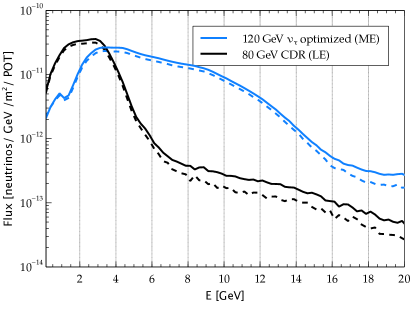
Figure 1: Comparison of the different beam tunes - the 80 GeV flux used in DUNE Conceptual Design Report (CDR) is referred to as LE flux while 120 GeV, $\nu_{\tau}$ optimized flux is referred to as the ME flux. The solid (dashed) curves represent the $\nu_{\mu}$ ($\bar{\nu}_{\mu}$) flux.

The simulations have been carried out using the widely used General Long Baseline Experiment Simulator (GLoBES) Huber et al. (2005, 2007) which solves the full three flavour neutrino propagation equations numerically using the Preliminary Reference Earth Model (PREM) Dziewonski and Anderson (1981) density profile of the Earth. The most recent DUNE configuration files from the DUNE collaboration Alion et al. (2016) have been used. A total runtime of 7 years with an on-axis 40 kiloton liquid argon far detector (FD) housed at the Homestake Mine in South Dakota over a baseline of 1300 km has been incorporated in the simulations.

We use two broad-band beam tunes : (i) the standard LE beam tune used in DUNE CDR Alion et al. (2016) and (ii) the ME beam tune optimized for $\nu_{\tau}$ appearance. The beams are obtained from a G4LBNF simulation Agostinelli et al. (2003); Allison et al. (2006) of the LBNF beam line using NuMI-style focusing. These two broad-band beam tunes are consistent with what could be achieved by the LBNF facility and we illustrate their comparison in Fig. 1. We have chosen a design for the ME beam that is nominally compatible with the space and infrastructure capabilities of the LBNF/DUNE beamline and that is based on a real working beamline design currently deployed in NuMI/NOvA. The beamline parameters assumed for the different design fluxes used in our analyses are listed in Table 1.

Parameter	LE (CPV optimized design)	ME ($\nu_{\tau}$ optimized)
Proton Beam energy	80 GeV	120 GeV
Proton Beam power	1.07 MW	1.2 MW
Protons on target (POT) per year	$1.47\times 10^{21}$	$1.10\times 10^{21}$
Focusing	3 horns	2 NuMI horns
	genetic optimisation	17 m apart
Horn Current	294 kA	230 kA
Decay pipe length	194 m	200 m
Decay pipe diameter	4 m	4 m

Table 1: Beamline parameters assumed for the different design fluxes used in our sensitivity calculations Acciarri et al. (2015); Alion et al. (2016); Abi et al. (2020a). The target is a thin graphite cylinder 2 interaction lengths long.

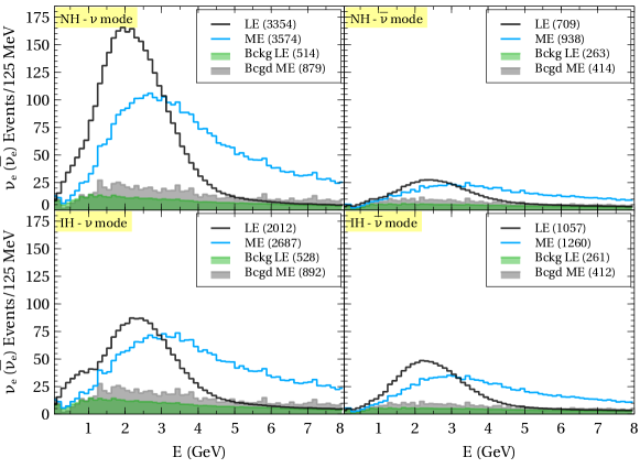
Figure 2: The ${\nu_{\mu}}\rightarrow{\footnotesize{\nu_{e}}}$ event spectra at DUNE are shown for different cases - the top (bottom) row corresponds to NH (IH) while the left (right) column corresponds to $\nu$ ($\bar{\nu}$) mode. The events obtained using the standard LE beam (the $\nu_{\tau}$-optimized ME beam) are depicted using black (blue) curves in each of the four panels. The total background corresponding with LE (ME) beam are shown as green (grey) shaded regions. In generating each of the event/background spectra, a total runtime of 7 years have been used. The numbers in the parentheses in the legends are the corresponding total number of events summed over the energy bins upto 8 GeV. The best-fit values of the oscillation parameters have been used to generate these event spectra (see Table 2).

In Fig. 2, we show the ${\nu_{\mu}}\rightarrow{\footnotesize{\nu_{e}}}$ (and $\bar{\nu}_{\mu}\rightarrow\bar{\nu}_{e}$) event spectra at DUNE when the beam tune is either the standard LE beam (black) or the $\nu_{\tau}$-optimized ME beam (blue). In order to make a fair comparison, the total runtime has been held fixed to 7 years in generating each of these four spectra. We note that though the LE flux gives an excess of events around $E\lesssim 3$ GeV, the ME beam offers complementarity by generating more events beyond $E\gtrsim 3$ GeV. In fact, for the chosen values of the parameters, the total number of events summed over the energy bins upto 8 GeV (as indicated in the figure), is slightly more for the ME beam with respect to the LE beam. This trend is visible for both $\nu$ and $\bar{\nu}$ modes irrespective of the choice of the hierarchy. In view of the above stated observations, we investigate whether a combination of LE and ME beam could lead to an improvement in the sensitivities to CPV, MH and octant of $\theta_{23}$ over and above what is expected from the LE beam alone. In Fig. 3, we show the ${\nu_{\mu}}\rightarrow{\nu_{\tau}}$ (and $\bar{\nu}_{\mu}\rightarrow\bar{\nu}_{\tau}$) event spectra at DUNE when the beam tune is either the standard LE beam (black) or the $\nu_{\tau}$-optimized ME beam (blue). It is worth mentioning that ME beam opens up the possibility to exploit this channel in addition to the ${\nu_{\mu}}\rightarrow{\footnotesize{\nu_{e}}}$ channel which further aids in improving the outcome of the sensitivity studies.

For classification of events using the two beam tunes, we follow Alion et. al. Alion et al. (2016). In the GLoBES configurations Alion et al. (2016), event classification was listed in distinct categories including electron neutrino appearance signal, ${\nu_{\mu}}\rightarrow{\footnotesize{\nu_{e}}}$ (CC), muon neutrino charged current signal, ${\nu_{\mu}}\rightarrow{\nu_{\mu}}$ (CC) as well as neutrino neutral current (NC) background, $\nu_{\mu}/\nu_{e}\to X$ (NC) both in appearance and disappearance modes. It should be noted that tau neutrino appearance ${\nu_{\mu}}\rightarrow{\nu_{\tau}}$ (CC) was included in Alion et al. (2016), but as a background. The corresponding systematics/efficiencies were provided as supplementary files in Alion et al. (2016). In the present study, we have incorporated a new category for tau neutrino appearance signal, ${\nu_{\mu}}\rightarrow{\nu_{\tau}}$ (CC). The backgrounds corresponding to this category include ${\nu_{\mu}}\rightarrow{\footnotesize{\nu_{e}}}$ (CC), ${\nu_{\mu}}\rightarrow{\nu_{\mu}}$ (CC) (due to the leptonic decay of tau lepton with branching fraction $\sim$ 35%) as well as NC background (due to the hadronic decay of the tau lepton with branching fraction $\sim$ 65%). Contamination due to wrong sign leptons is also taken into account as background.

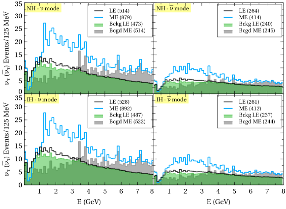
Figure 3: The ${\nu_{\mu}}\rightarrow{\nu_{\tau}}$ event spectra at DUNE are shown for different cases - the top (bottom) row corresponds to NH (IH) while the left (right) column corresponds to $\nu$ ($\bar{\nu}$) mode. The events obtained using the standard LE beam (the $\nu_{\tau}$-optimized ME beam) are depicted using black (blue) curves in each of the four panels. The total background corresponding with LE (ME) beam are shown as green (grey) shaded regions. In generating each of the event/background spectra, a total runtime of 7 years have been used. The numbers in the parentheses in the legends are the corresponding total number of events summed over the energy bins upto 8 GeV. The best-fit values of the oscillation parameters have been used to generate these event spectra (see Table 2).

IV Analysis method

Parameter	Best-fit-value	3$\sigma$ interval	$1\sigma$ uncertainty
$\theta_{12}$ [Deg.]	34.3	31.4 - 37.4	2.9%
$\theta_{13}$ (NH) [Deg.]	8.58	8.16 - 8.94	1.5%
$\theta_{13}$ (IH) [Deg.]	8.63	8.21 - 8.99	1.5%
$\theta_{23}$ (NH) [Deg.]	48.8	41.63 - 51.32	3.5%
$\theta_{23}$ (IH) [Deg.]	48.8	41.88 - 51.30	3.5%
$\Delta m_{21}^{2}$ [$\text{eV}^{2}$]	$7.5\times 10^{-5}$	[6.94 - 8.14]$\times 10^{-5}$	2.7%
$\Delta m_{31}^{2}$ (NH) [$\text{eV}^{2}$]	$+2.56\times 10^{-3}$	[2.46 - 2.65] $\times 10^{-3}$	1.2%
$\Delta m_{31}^{2}$ (IH) [$\text{eV}^{2}$]	$-2.46\times 10^{-3}$	-[2.37 - 2.55]$\times 10^{-3}$	1.2%
$\delta$ (NH) [Rad.]	$-0.8\pi$	$[-\pi,0]\cup[0.8\pi,\pi]$	$-$
$\delta$ (IH) [Rad.]	$-0.46\pi$	$[-0.86\pi,-0.1\pi]$	$-$

Table 2: Standard oscillation parameters and their uncertainties used in our study. The values were taken from the global fit analysis in de Salas et al. (2020). If the $3\sigma$ upper and lower limit of a parameter is $x_{u}$ and $x_{l}$ respectively, the $1\sigma$ uncertainty is $(x_{u}-x_{l})/3(x_{u}+x_{l})\%$ Abi et al. (2020a).

To estimate the sensitivities of DUNE to mass hierarchy (MH), CP violation (CPV) and octant of $\theta_{23}$, we perform the standard $\Delta\chi^{2}$ analysis. Even though all results are produced numerically with the help of GLoBES software, in order to gain insight, let us examine the analytical form of the $\Delta\chi^{2}$ .

$$\Delta\chi^{2}(p^{\text{true}})=\underset{p^{\text{test}},\eta}{\text{Min}}\Bigg{[} 2\sum_{y}^{\text{flux}}\sum_{x}^{\text{mode}}\sum_{j}^{\text{channel}}\sum_{i}^{\text{bin}}\Bigg{\{}N_{ijxy}^{\text{test}}(p^{\text{test}};\eta)-N_{ijxy}^{\text{true}}(p^{\text{true}})+N_{ijxy}^{\text{true}}(p^{\text{true}})\ln\frac{N_{ijxy}^{\text{true}}(p^{\text{true}})}{N_{ijxy}^{\text{test}}(p^{\text{test}};\eta)}\Bigg{\}}$$

$$+\sum_{l}\frac{(p^{\text{true}}_{l}-p^{\text{test}}_{l})^{2}}{\sigma_{p_{l}}^{2}}+\sum_{k}\frac{\eta_{k}^{2}}{\sigma_{k}^{2}}\Bigg{]},$$ (18)

where $N^{\text{true}}$ and $N^{\text{test}}$ are the set of true and test events respectively. Index $i$ is summed over the energy bins in the range $0-20$ GeV. The indices $j$ and $x$ are summed over the channels (${\nu_{\mu}}\rightarrow{\footnotesize{\nu_{e}}},{\nu_{\mu}}\rightarrow{\nu_{\mu}},{\nu_{\mu}}\rightarrow{\nu_{\tau}}$) and the modes ($\nu$ and $\bar{\nu}$) respectively. The sum over the index $y$ takes into account the multiple fluxes (LE and ME tuned beams), whenever multiple fluxes are used. The term inside the curly braces in Eq. IV is the statistical part of $\Delta\chi^{2}$. The term $(N^{\text{test}}-N^{\text{true}})$ takes into account the algebraic difference while the third term inside the curly braces considers the fractional difference between the test and true sets of events. $p^{\text{true}}$ and $p^{\text{test}}$ are the set of true and test oscillation parameters respectively and $\sigma_{p_{l}}$ is the uncertainty in the prior measurement of the parameter $p_{l}$. The values of the true or best-fit oscillation parameters and their uncertainties as used in the present analysis are tabulated in Table 2. The index $l$ is summed over the number of test oscillation parameters to be marginalized. This is known as the prior term. The index $k$ is summed over the number of systematics/nuisance parameters present. This way of treating the nuisance parameters in the $\Delta\chi^{2}$ calculation is known as the method of pulls Huber et al. (2002); Fogli et al. (2002); Gonzalez-Garcia and Maltoni (2004); Gandhi et al. (2007). Regarding the systematics, the $\nu_{e}$ and $\bar{\nu}_{e}$ signal modes have a normalization uncertainties of $2\%$ each, whereas the $\nu_{\mu}$ and $\bar{\nu}_{\mu}$ signals have a normalization uncertainty of $5\%$ each. The $\nu_{\tau}$ and $\bar{\nu}_{\tau}$ signals have a normalization uncertainties of $20\%$ each. The background normalization uncertainties vary from $5\%-20\%$ and include correlations among various sources of background (coming from beam $\nu_{e}/\bar{\nu}_{e}$ contamination, flavour misidentification, NC and $\nu_{\tau}$). The final estimate of $\Delta\chi^{2}$ which is thus a function of the true values of the oscillation parameters, is obtained after a minimization (i.e., marginalization over the $3\sigma$ range of values) over the set of test parameters ($p^{\text{test}}$) and the set of systematics ($\eta$). Technically this $\Delta\chi^{2}$ is the frequentist method of hypotheses testing Fogli et al. (2002); Qian et al. (2012).

For calculating the sensitivity to MH, we marginalise the test $\Delta m_{31}^{2}$ in the opposite hierarchy in the $3\sigma$ range of values. Test parameters $\theta_{23},\theta_{13}$ are marginalized over their $3\sigma$ ranges, while the CP phase $\delta$ is marginalized over the full range of $[-\pi,\pi]$. For the sensitivity to CPV, the test $\delta$ is allowed to marginalize over only the CP conserving values of 0 and $\pi$ while the true $\delta$ can take any value in the range $[-\pi,\pi]$. The other test parameters in that case ($\Delta m_{31}^{2},\theta_{13},\theta_{23}$) are marginalized over the $3\sigma$ range. For the calculation of the sensitivity to $\theta_{23}$ octant, the test $\theta_{23}$ is marginalized in the opposite octant. The marginalization of the test parameters $\Delta m_{31}^{2}$ and $\theta_{13}$ are carried out over their respective $3\sigma$ range, while that of test $\delta$ is done in the whole allowed range of $[-\pi,\pi]$.

We keep the total runtime at DUNE fixed at 7 years and numerically calculate $\Delta\chi^{2}$ as a function of true $\delta\in[-\pi,\pi]$ after varying the distribution of runtime (with a stepsize of 0.5 year) among the following four variables :

• Runtime using LE beam and in neutrino mode ($\mathcal{R}_{\text{\tiny{LE}}}$)

• Runtime using LE beam and in anti-neutrino mode ($\mathcal{\overline{R}}_{\text{\tiny{LE}}}$)

• Runtime using ME beam and in neutrino mode ($\mathcal{R}_{\text{\tiny{ME}}}$)

• Runtime using ME beam and in anti-neutrino mode ($\mathcal{\overline{R}}_{\text{\tiny{ME}}}$).

Note that, since $\mathcal{R}_{\text{\tiny{LE}}}+\mathcal{\overline{R}}_{\text{\tiny{LE}}}+\mathcal{R}_{\text{\tiny{ME}}}+\mathcal{\overline{R}}_{\text{\tiny{ME}}}=7$ (years), only three of the above variables are independent. In order to figure out the optimized runtime combination, we define that combination of $\mathcal{R}_{\text{\tiny{LE}}},\mathcal{\overline{R}}_{\text{\tiny{LE}}},\mathcal{R}_{\text{\tiny{ME}}},\mathcal{\overline{R}}_{\text{\tiny{ME}}}$ which gives the largest area under the sensitivity curve in the ($\Delta\chi^{2}$-true $\delta$) plane for all three unknowns : CPV, MH and octant of $\theta_{23}$. We refer to the optimized runtime combination estimated in this manner as $R_{\text{\tiny{CPV}}}^{\text{area}},R_{\text{\tiny{MH}}}^{\text{area}}$ or $R_{\text{\tiny{OCT}}}^{\text{area}}$ respectively for the three quantities. Additionally, for the CPV case, we define another optimized combination of runtimes (i.e., $\mathcal{R}_{\text{\tiny{LE}}},\mathcal{\overline{R}}_{\text{\tiny{LE}}},\mathcal{R}_{\text{\tiny{ME}}},\mathcal{\overline{R}}_{\text{\tiny{ME}}}$) that resolves CPV above $3\sigma$ for the largest fraction of true $\delta$ parameter space. We refer to this optimized combination as $R_{\text{\tiny{CPV}}}^{\text{fraction}}$.

V Optimized runtime combinations : Sensitivity to CPV, MH and octant of $\theta_{23}$

We present our main results by estimating the optimized runtime combinations of $(\mathcal{R}_{\text{\tiny{LE}}},\mathcal{\overline{R}}_{\text{\tiny{LE}}},\mathcal{R}_{\text{\tiny{ME}}},\mathcal{\overline{R}}_{\text{\tiny{ME}}})$ that give the best sensitivities to resolve CPV, MH and octant of $\theta_{23}$. In what follows, we obtain the optimal combinations of runtimes and which are reported as $(\mathcal{R}_{\text{\tiny{LE}}}+\mathcal{\overline{R}}_{\text{\tiny{LE}}}+\mathcal{R}_{\text{\tiny{ME}}}+\mathcal{\overline{R}}_{\text{\tiny{ME}}})$ for the three different questions addressed in the present work.

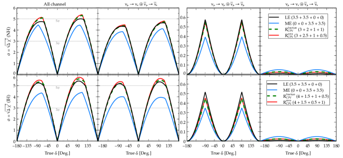
Figure 4: The sensitivity to CPV at DUNE are shown with the variation of true $\delta$, for optimized runtime combination for LE+ME, - found either by maximizing the area under the sensitivity curve (solid red) or by maximizing the fraction of true $\delta$ space for which the sensitivity is above $3\sigma$ (dashed green). The sensitivities obtained for LE only(black) or ME only (blue) beam with equal runtime in $\nu$ and $\bar{\nu}$ modes are also shown. The legends signify the runtime combination for each case in the form ($\mathcal{R}_{\text{\tiny{LE}}}+\mathcal{\overline{R}}_{\text{\tiny{LE}}}+\mathcal{R}_{\text{\tiny{ME}}}+\mathcal{\overline{R}}_{\text{\tiny{ME}}}$). The top (bottom) row depicts the case of true NH (IH). The first column shows the combined results considering all channels while the second, third and fourth column shows the contributions from the individual channels ${\nu_{\mu}}\rightarrow{\footnotesize{\nu_{e}}},{\nu_{\mu}}\rightarrow{\nu_{\mu}}$ and ${\nu_{\mu}}\rightarrow{\nu_{\tau}}$ respectively.

Sensitivity to CP violation :- In Fig. 4, we illustrate the optimized runtime combination of $(\mathcal{R}_{\text{\tiny{LE}}}+\mathcal{\overline{R}}_{\text{\tiny{LE}}}+\mathcal{R}_{\text{\tiny{ME}}}+\mathcal{\overline{R}}_{\text{\tiny{ME}}})$ that give the best sensitivity to CPV at DUNE by (a) maximizing the area under the sensitivity curve (red solid), and (b) maximizing the fraction of true $\delta$ parameter space that resolves the CPV sensitivity above $3\sigma$ (green dashed). For comparison, we also show the CPV sensitivities by using only the standard LE beam (black) or the ME beam only (blue) - the distribution of runtime being equally (3.5 years) shared between the $\nu$ and $\bar{\nu}$ modes for each case. The first column shows the main results where (neutrino and antineutrino) contributions from all three oscillation channels (${\nu_{\mu}}\rightarrow{\footnotesize{\nu_{e}}},{\nu_{\mu}}\rightarrow{\nu_{\mu}},{\nu_{\mu}}\rightarrow{\nu_{\tau}}$) are considered. The second, third and fourth column shows the (neutrino and antineutrino) contribution from the individual channels ${\nu_{\mu}}\rightarrow{\footnotesize{\nu_{e}}},{\nu_{\mu}}\rightarrow{\nu_{\mu}}$ and ${\nu_{\mu}}\rightarrow{\nu_{\tau}}$ respectively. The top (bottom) row depicts the case of true NH (IH).

For NH, the sensitivity to CPV at the best runtime combination ($R_{\text{\tiny{CPV}}}^{\text{area}}$ or $R_{\text{\tiny{CPV}}}^{\text{fraction}}$) is enhanced beyond $5\sigma$ around the CP violating values ($\approx\pm\pi/2$) of true $\delta$. The $5\sigma$ reach of the sensitivity to CPV was otherwise not achievable using only the standard LE beam or the ME beam with a runtime of (3.5 years $\nu$ mode + 3.5 years $\bar{\nu}$ mode for either of the beams). For the NH scenario, an optimized runtime combination $(R_{\text{\tiny{CPV}}}^{\text{area}}\equiv{\bf{3+2.5+1+0.5)}}$ estimated by maximizing the area of implies that DUNE needs to run for a total of (a) 5.5 years using the LE beam (with 3 years in $\nu$ mode and 2.5 years in $\bar{\nu}$ mode), and (b) 1.5 years using the ME beam (with 1 year in $\nu$ mode and 0.5 year  in $\bar{\nu}$ mode). It should be noted that the optimized runtime combination obtained by maximizing the fraction is similar to that obtained while maximizing the area.

For IH, it is found that the CP violation sensitivity does not improve much when we use a combination of beam tunes (LE+ME). This is because the sensitivity generated by LE beam is somewhat higher for IH than for NH which gives less scope of improvement.

It is worth mentioning that most of the contribution to the CP violation sensitivity arises from the ${\nu_{\mu}}\rightarrow{\footnotesize{\nu_{e}}}$ appearance channel. In Appendix A, we try to explain why this is the dominant channel while the other two channels (i.e., ${\nu_{\mu}}\rightarrow{\nu_{\mu}}$ and ${\nu_{\mu}}\rightarrow{\nu_{\tau}}$) give rise to small contribution (see also Masud et al. (2016); Masud and Mehta (2016a)).

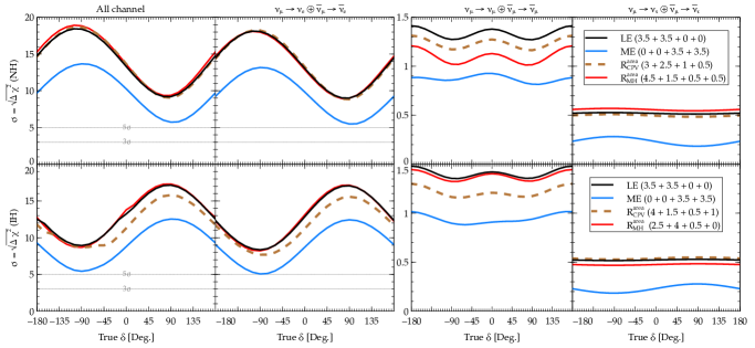
Figure 5: The sensitivities to MH at DUNE are shown with the variation of true $\delta$, for optimized runtime combination for LE+ME, - found by maximizing the area under the sensitivity curve (solid red). The sensitivities obtained for LE only(black) or ME only (blue) beam are also shown with equal runtime in $\nu$ and $\bar{\nu}$ modes. The legends signify the runtime combination for each case in the form ($\mathcal{R}_{\text{\tiny{LE}}}+\mathcal{\overline{R}}_{\text{\tiny{LE}}}+\mathcal{R}_{\text{\tiny{ME}}}+\mathcal{\overline{R}}_{\text{\tiny{ME}}}$). For comparison, the MH sensitivities corresponding to $R_{\text{\tiny{CPV}}}^{\text{area}}$ are also shown (dashed brown). The legends signify the runtime combination for each case in the form ($\mathcal{R}_{\text{\tiny{LE}}}+\mathcal{\overline{R}}_{\text{\tiny{LE}}}+\mathcal{R}_{\text{\tiny{ME}}}+\mathcal{\overline{R}}_{\text{\tiny{ME}}}$). The top (bottom) row depicts the case of true NH (IH). The first column shows the combined results considering all channels while the second, third and fourth column shows the contributions from the individual channels ${\nu_{\mu}}\rightarrow{\footnotesize{\nu_{e}}},{\nu_{\mu}}\rightarrow{\nu_{\mu}}$ and ${\nu_{\mu}}\rightarrow{\nu_{\tau}}$ respectively.

Sensitivity to MH :- In Fig. 5, we illustrate the optimized runtime combination (red curves) of $(\mathcal{R}_{\text{\tiny{LE}}}+\mathcal{\overline{R}}_{\text{\tiny{LE}}}+\mathcal{R}_{\text{\tiny{ME}}}+\mathcal{\overline{R}}_{\text{\tiny{ME}}})$ that gives the best MH sensitivity at DUNE. For the sake of comparison, we additionally show the MH sensitivities (dashed brown) corresponding to the best runtime combination ($R_{\text{\tiny{CPV}}}^{\text{area}}$) estimated for CPV sensitivity. We also show the sensitivities to MH by using only the standard LE beam (black) or the ME beam (blue), the distribution of runtime being equally (3.5 year) shared between the $\nu$ and $\bar{\nu}$ modes. The MH sensitivity of DUNE using only the standard LE beam is already very high for the entire range of values of the CP phase and $R_{\text{\tiny{MH}}}^{\text{area}}$ combination does not offer much improvement. Since the contribution to MH sensitivity mainly comes from around the first oscillation maximum ($2-2.5$ GeV) for which the LE beam offers best statistics, the use of ME beam is not expected to lead to much improvement. The best MH runtime combination is (${\bf{4.5+1.5+0.5+0.5}}$) for NH and ($2.5+4+0.5+0$) for IH. For this particular question also, the ${\nu_{\mu}}\rightarrow{\nu_{\mu}}$ and ${\nu_{\mu}}\rightarrow{\nu_{\tau}}$ channels do not contribute significantly (see Appendix A and Masud and Mehta (2016b) to get an insight into the typical shape of the MH sensitivities at long baseline experiments as well as for an understanding of the role of different oscillation channels). As can be seen from Fig. 5, we have also estimated the MH sensitivity corresponding to $R_{\text{\tiny{CPV}}}^{\text{area}}$ (brown dashed curve). It is seen that for NH, it is almost the same as that of $R_{\text{\tiny{MH}}}^{\text{area}}$ while for IH it is lower than the standard sensitivity (black curve). Interestingly, we observe that, for $R_{\text{\tiny{MH}}}^{\text{area}}$, $\mathcal{R}_{\text{\tiny{LE}}}$ plays a dominant role when the hierarchy is normal while $\mathcal{\overline{R}}_{\text{\tiny{LE}}}$ plays a dominant role for the IH case.

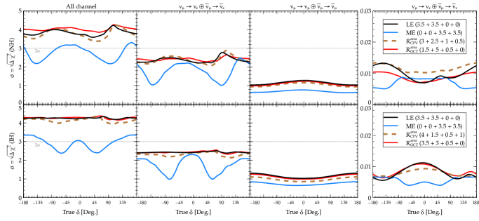
Figure 6: The sensitivities to $\theta_{23}$-octant degeneracy (true octant being HO) at DUNE are shown with the variation of true $\delta$, for optimized runtime combination for LE+ME, - found by maximizing the area under the sensitivity curve (solid red). The sensitivities obtained for LE only(black) or ME only (blue) beam are also shown with equal runtime in $\nu$ and $\bar{\nu}$ modes. The legends signify the runtime combination for each case in the form ($\mathcal{R}_{\text{\tiny{LE}}}+\mathcal{\overline{R}}_{\text{\tiny{LE}}}+\mathcal{R}_{\text{\tiny{ME}}}+\mathcal{\overline{R}}_{\text{\tiny{ME}}}$). For comparison, the octant sensitivities corresponding to $R_{\text{\tiny{CPV}}}^{\text{area}}$ are also shown (dashed brown). The legends signify the runtime combination for each case in the form ($\mathcal{R}_{\text{\tiny{LE}}}+\mathcal{\overline{R}}_{\text{\tiny{LE}}}+\mathcal{R}_{\text{\tiny{ME}}}+\mathcal{\overline{R}}_{\text{\tiny{ME}}}$). The top (bottom) row depicts the case of true NH (IH). The first column shows the combined results considering all channels while the second, third and fourth column shows the contributions from the individual channels ${\nu_{\mu}}\rightarrow{\footnotesize{\nu_{e}}},{\nu_{\mu}}\rightarrow{\nu_{\mu}}$ and ${\nu_{\mu}}\rightarrow{\nu_{\tau}}$ respectively.

Sensitivity to octant of $\theta_{23}$:- We next compute the optimized runtime combinations of $(\mathcal{R}_{\text{\tiny{LE}}}+\mathcal{\overline{R}}_{\text{\tiny{LE}}}+\mathcal{R}_{\text{\tiny{ME}}}+\mathcal{\overline{R}}_{\text{\tiny{ME}}})$ that gives the best sensitivity to $\theta_{23}$ octant at DUNE when the true octant is HO ($\theta_{23}$ = $48.8^{\circ}$). In Fig. 6, the top (bottom) row depict the case of NH (IH), while the second, third and fourth columns show the roles of individual oscillation channels. We observe in Fig. 6 that the best runtime combination of (${\bf{1.5+5+0.5+0}}$) for NH scenario underscores the importance of $\bar{\nu}$ runtimes and this optimized combination improves this sensitivity significantly. This is apparent for IH scenario ($2.5+3+1.5+0$) as well, albeit in a less prominent manner. We also note that unlike the case of CPV and MH, the ${\nu_{\mu}}\rightarrow{\nu_{\mu}}$ ($\bar{\nu}_{\mu}\rightarrow\bar{\nu}_{\mu}$) disappearance channel contributes substantially to the octant sensitivities. The ${\nu_{\mu}}\rightarrow{\nu_{\tau}}$ ($\bar{\nu}_{\mu}\rightarrow\bar{\nu}_{\tau}$) channel, on the other hand, practically has no role (see Appendix A). We also show the octant sensitivities by using only the standard LE beam (black) or the ME beam only (blue), the distribution of runtime being equally shared among the $\nu$ and $\bar{\nu}$ modes. Additionally, for the sake of comparison, the dashed brown curves illustrate the octant sensitivity obtained corresponding to $R_{\text{\tiny{CPV}}}^{\text{area}}$.

Tab. 3 summarises the results for estimated optimized combinations with respect to CPV sensitivity, MH sensitivity and sensitivity to the octant of $\theta_{23}$ respectively.

Sensitivity to	Optimization combination	NH	IH
		$(\mathcal{R}_{\text{\tiny{LE}}}+\mathcal{\overline{R}}_{\text{\tiny{LE}}}+\mathcal{R}_{\text{\tiny{ME}}}+\mathcal{\overline{R}}_{\text{\tiny{ME}}})$	$(\mathcal{R}_{\text{\tiny{LE}}}+\mathcal{\overline{R}}_{\text{\tiny{LE}}}+\mathcal{R}_{\text{\tiny{ME}}}+\mathcal{\overline{R}}_{\text{\tiny{ME}}})$
		(in years)	(in years)
CPV	$R_{\text{\tiny{CPV}}}^{\text{area}}$	$3+2.5+1+0.5$	$4+1.5+0.5+1$
	$R_{\text{\tiny{CPV}}}^{\text{fraction}}$	$3+2+1+1$	$4+1.5+1+0.5$
MH	$R_{\text{\tiny{MH}}}^{\text{area}}$	$4.5+1.5+0.5+0.5$	$2.5+4+0.5+0$
Octant of $\theta_{23}$	$R_{\text{\tiny{OCT}}}^{\text{area}}$ (HO)	$1.5+5+0.5+0$	$3.5+3+0.5+0$

Table 3: Optimized runtime combinations for sensitivity to CPV, MH and octant of $\theta_{23}$ at DUNE.

VI Sensitivity to the choice of optimal combination

Having completed the task of estimating the optimal combination of runtime that yields the best sensitivity to the three unknowns, we would now like to pose the following question. How sensitive are we to the choice of optimal combination or what direction can we take (in our choice of runtime combinations) in case we have difficulty in implementation of the particular runtime combination. We address these questions in the present section.

We examine the different runtime combinations and analyze how the results improve (i.e., how the area under the $\Delta\chi^{2}$ curve as a function of true $\delta$ for CPV, MH, octant increases) for different runtime combinations. In Fig. 7, we show the heatmap of the area (normalized) under the sensitivity curves (in the $\Delta\chi^{2}$-true $\delta$ plane) for all the runtime combinations ($\mathcal{R}_{\text{\tiny{LE}}}+\mathcal{\overline{R}}_{\text{\tiny{LE}}}+\mathcal{R}_{\text{\tiny{ME}}}+\mathcal{\overline{R}}_{\text{\tiny{ME}}}$) considered. The three columns show the case of CPV, MH and octant sensitivities, while the top (bottom) row depicts the NH (IH) scenario. The lower triangular portion (red) shows the effect of the $\mathcal{R}_{\text{\tiny{LE}}}$ and $\mathcal{\overline{R}}_{\text{\tiny{LE}}}$ components of the runtime combination along the bottom horizontal axis and the left vertical axis respectively. The upper triangular portion (blue) shows the effect of the $\mathcal{R}_{\text{\tiny{ME}}}$ and $\mathcal{\overline{R}}_{\text{\tiny{ME}}}$ components of the runtime combination along the top horizontal axis and the right vertical axis respectively. The lighter (darker) shades of the colours imply better (worse) sensitivity. Thus, any runtime combination read off Fig. 7 consists of two parts: ($\mathcal{R}_{\text{\tiny{LE}}}+\mathcal{\overline{R}}_{\text{\tiny{LE}}}$) in the red lower triangular region, and the corresponding ($\mathcal{R}_{\text{\tiny{ME}}}+\mathcal{\overline{R}}_{\text{\tiny{ME}}}$) in the blue upper triangular region such that $\mathcal{R}_{\text{\tiny{LE}}}+\mathcal{\overline{R}}_{\text{\tiny{LE}}}+\mathcal{R}_{\text{\tiny{ME}}}+\mathcal{\overline{R}}_{\text{\tiny{ME}}}=7$. The black dot indicates the case of standard runtime using only LE beam (${\bf{3.5+3.5+0+0}}$). The optimized runtime combinations ($R_{\text{\tiny{CPV}}}^{\text{area}},R_{\text{\tiny{MH}}}^{\text{area}},R_{\text{\tiny{OCT}}}^{\text{area}}$) giving the best sensitivities are marked with a pair of green, brown and magenta dots in the three columns respectively. For comparison, the combination $R_{\text{\tiny{CPV}}}^{\text{area}}$ (green dot) is also marked for the case of MH and octant sensitivities (i.e., second and third column). The fact that the lighter shaded regions ae located away from the combination represented by the black dot clearly indicates how the result improves when one combines the ME beam (i.e., nonzero $\mathcal{R}_{\text{\tiny{ME}}}$ and $\mathcal{\overline{R}}_{\text{\tiny{ME}}}$) with the LE beam. For MH (2nd column), interestingly more $\mathcal{R}_{\text{\tiny{LE}}}$ facilitates the improvement of the sensitivities for true NH case, while $\mathcal{\overline{R}}_{\text{\tiny{LE}}}$ is slightly favoured for true IH. For octant sensitivity (third column of Fig. 7) it is clear that for NH, $R_{\text{\tiny{OCT}}}^{\text{area}}$ is dominated by $\mathcal{\overline{R}}_{\text{\tiny{LE}}}$, while for IH, both $\mathcal{R}_{\text{\tiny{LE}}}$ and $\mathcal{\overline{R}}_{\text{\tiny{LE}}}$ play equally important roles. Fig. 7 also helps to highlight the need for $\bar{\nu}$ mode runs in probing the $\theta_{23}$ octant sensitivity.

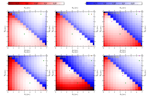
Figure 7: Heatmap of the normalized area under the sensitivity curves (in the [$\Delta\chi^{2}$-true $\delta$] plane) for all the runtime combinations considered in the context of CPV, MH and $\theta_{23}$ octant sensitivities in the three columns respectively. The top (bottom) row depicts the case of true NH (IH). The four components of the runtime combination are shown along the four sides of each panel. The lighter (darker) shades of the colours imply better (worse) sensitivity. We mark the case of standard runtime ($\mathcal{R}_{\text{\tiny{LE}}}+\mathcal{\overline{R}}_{\text{\tiny{LE}}}+\mathcal{R}_{\text{\tiny{ME}}}+\mathcal{\overline{R}}_{\text{\tiny{ME}}}=3.5+3.5+0+0$) with a black dot. The optimized runtime combinations summarised in Tab. 3 ($R_{\text{\tiny{CPV}}}^{\text{area}},R_{\text{\tiny{MH}}}^{\text{area}},R_{\text{\tiny{OCT}}}^{\text{area}}$) giving the best sensitivities are marked with green, brown and magenta dots in the three columns respectively. The combination $R_{\text{\tiny{CPV}}}^{\text{area}}$ (green dot) is also marked for the case of MH and octant sensitivities (i.e., second and third column) for comparison.

VII Summary

CP violation, MH and octant of $\theta_{23}$ are the crucial unknowns and current and future long baseline experiments such as DUNE are planned to address these questions. In the basic configuration, it is assumed that DUNE would have a runtime of 7 years (distributed equally in the $\nu$ and $\bar{\nu}$ mode) with the standard LE beam. The LE beam that is often used in DUNE simulations has a peak around $2-3$ GeV (the first oscillation maximum for ${\nu_{\mu}}\rightarrow{\footnotesize{\nu_{e}}}$ transition probability) but very sharply falls off at $E\gtrsim 4$ GeV. Consequently, the number of events beyond $4$ GeV rapidly becomes smaller, providing very little statistics. In the present work, we propose to use a higher energy, ME beam that has a substantial flux even beyond 4 GeV in addition to the LE beam and ask whether this can offer any improvement to the standard sensitivity reach of DUNE in answering question pertaining to CPV, MH and octant of $\theta_{23}$.

Keeping the total runtime fixed to 7 years, we have distributed the total runtime among the $\nu$ and $\bar{\nu}$ modes with the possibility of utilizing the different beam tunes, LE and ME. We have chosen a design for the ME beam that is nominally compatible with the space and infrastructure capabilities of the LBNF/DUNE beamline and that is based on a real working beamline design currently deployed in NuMI/NOvA. In each of these sensitivity analyses, we have considered the (neutrino and antineutrino) contributions of all three oscillation channels ${\nu_{\mu}}\rightarrow{\footnotesize{\nu_{e}}},{\nu_{\mu}}\rightarrow{\nu_{\mu}}$ and ${\nu_{\mu}}\rightarrow{\nu_{\tau}}$ and shown the contribition of the individual channels to the overall sensitivity. We specify the different runtimes using different beam tunes and modes as $\mathcal{R}_{\text{\tiny{LE}}},\mathcal{\overline{R}}_{\text{\tiny{LE}}},\mathcal{R}_{\text{\tiny{ME}}},\mathcal{\overline{R}}_{\text{\tiny{ME}}}$. The optimized combinations $\mathcal{R}_{\text{\tiny{LE}}}+\mathcal{\overline{R}}_{\text{\tiny{LE}}}+\mathcal{R}_{\text{\tiny{ME}}}+\mathcal{\overline{R}}_{\text{\tiny{ME}}}$ that give the best sensitivities to CPV, MH and octant of $\theta_{23}$ are then evaluated.

Our results are reported in Sec. V. In Fig. 4, we found that a runtime combination of ${\bf{(3+2.5+1+0.5)}}$ gives the best sensitivity to CP violation if the hierarchy is normal. Also, the sensitivity can reach beyond $5\sigma$, which was otherwise not possible with the standard DUNE configuration with LE beam alone near $\delta\simeq\pm\pi/2$ (maximal CPV). In addition to resolving CPV, this particular optimized runtime combination also offers high sensitivity to resolve the MH (see Fig. 5) and octant of $\theta_{23}$ (see Fig. 6). For MH and octant of $\theta_{23}$, the optimized runtime combinations providing the best sensitivities are found to be ${\bf{(4.5+1.5+0.5+0.5)}}$ and ${\bf{(1.5+5+0.5+0)}}$ respectively (assuming the hierarchy is normal). Finally, Tab. 3 summarises the results for estimated optimized combinations w.r.t. CPV sensitivity, MH sensitivity and senstivity to the octant of $\theta_{23}$ respectively.

This study, therefore, underscores the availability of the room for improvement within the DUNE experimental configuration by using a combination of runtime in the $\nu$ and $\bar{\nu}$ mode, exploiting two different (LE and ME) beam tunes. This suggested runtime configuration with the two available beam tunes will eventually help DUNE to answer, with more robustness, its main goals pertaining to leptonic CP violation, determination of MH and octant of $\theta_{23}$.

We would like to mention that our phenomenological study is concerned primarily with bringing out the physics capabilities introduced by the ME beam tune. Consideration of the cost as well as other detailed technical changes needed to replace the current beamline design with the ME tune proposed above is outside the purview of this paper. It may be worth mentioning that LBNF/DUNE full CP violation sensitivity assumes an upgrade to a 2.4 MW beam which will require a complete redesign of the targeting and focusing system and thus the facility is designed with the ability to accommodate different targetry and focusing designs.

Appendix A: Role of different channels in probability

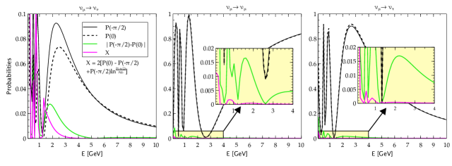
Figure 8: Comparison of probabilities (solid and dashed black) and their differences (green) for the three channels ${\nu_{\mu}}\rightarrow{\footnotesize{\nu_{e}}}$ (first panel), ${\nu_{\mu}}\rightarrow{\nu_{\mu}}$ (second) and ${\nu_{\mu}}\rightarrow{\nu_{\tau}}$ (third). A $\Delta\chi^{2}$-like quantity $X$ (magenta) in the probability level gives a measure of the contributions of these three channels to the sensitivity to CPV.

Here we discuss how the individual channels (${\nu_{\mu}}\rightarrow{\footnotesize{\nu_{e}}},{\nu_{\mu}}\rightarrow{\nu_{\mu}},{\nu_{\mu}}\rightarrow{\nu_{\tau}}$) contribute in the probability level in probing the questions related to CPV, MH and the octant of $\theta_{23}$ at the DUNE baseline of 1300 km. The $\Delta\chi^{2}$ estimation for CPV in Fig. 4 gives a numerical measure of the difference between the CP conserving value (test $\delta=0$ or $\pi$) and all values of true $\delta$ ($\in[-\pi,\pi]$) and is maximum around true $\delta\approx\pm\pi/2$. In Fig. 8, we do a probability analysis by plotting $P_{\mu\beta}$ ($\beta=e,\mu,\tau$) for $\delta=-\pi/2$ (solid black), $0$ (dashed black) and their absolute difference (green). Finally we also show a $\Delta\chi^{2}$-like quantity $X$ (magenta) defined in the probability level following the statistical part of Eq. IV. For Fig. 8, the explicit definition of this quantity is,

$$X_{\text{CPV}}=2\bigg{[}P_{\mu\beta}(0)-P_{\mu\beta}(-\pi/2)+P_{\mu\beta}(-\pi/2)\ln\frac{P_{\mu\beta}(-\pi/2)}{P_{\mu\beta}(0)}\bigg{]},$$ (A1)

where the argument within the parentheses are the values of the CP phase $\delta$. Fig. 8 shows that though the magnitudes of the difference of probabilities (green) are in the similar ballpark for all the three channels, the contribution to the $\Delta\chi^{2}$-like quantity $X$ (magenta) mainly comes from the ${\nu_{\mu}}\rightarrow{\footnotesize{\nu_{e}}}$ channel. This is because the fractional difference of the probabilities (which dominates the estimation of $\Delta\chi^{2}$) in the ${\nu_{\mu}}\rightarrow{\footnotesize{\nu_{e}}}$ channel is much higher,- owing to the small magnitudes of $P_{\mu e}$. As is clear from the insets in Fig. 8, this fractional difference (magenta) is tiny for the ${\nu_{\mu}}\rightarrow{\nu_{\mu}}$ and ${\nu_{\mu}}\rightarrow{\nu_{\tau}}$ channels.

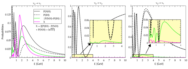
Figure 9: Similar to Fig. 8 but for contribution to explore the MH degeneracy.

Similarly, in Fig. 9, we analyse the contributions of the three channels in probing the MH degeneracy. For the two opposite hierarchies NH and IH, we show $P_{\mu\beta}$ (solid black and dashed black), their difference (green) and the $\Delta\chi^{2}$-like quantity (magenta) defined below:

$$X_{\text{MH}}=2\bigg{[}P_{\mu\beta}(IH)-P_{\mu\beta}(NH)+P_{\mu\beta}(NH)\ln\frac{P_{\mu\beta}(NH)}{P_{\mu\beta}(IH)}\bigg{]}.$$ (A2)

We take the CP phase to be $-\pi/2$ here. It can be easily observed that $X$ is again dominated by the ${\nu_{\mu}}\rightarrow{\footnotesize{\nu_{e}}}$ channel, while the ${\nu_{\mu}}\rightarrow{\nu_{\mu}}$ channel gives almost no contribution. Interestingly, though the difference of $P_{\mu\tau}$ for NH and IH (i.e., green curve) is very similar in magnitude with that of $P_{\mu e}$, the large value of $P_{\mu\tau}$ makes the fractional difference and consequently the value of the $\Delta\chi^{2}$-like quantity $X$ insignificant.

Finally the probability level analyses for $\theta_{23}$-octant degeneracy is illustrated in Fig. 10. The $\Delta\chi^{2}$-like quantity $X$ is defined as follows.

$$X_{\text{OCT}}=2\bigg{[}P_{\mu\beta}(LO)-P_{\mu\beta}(HO)+P_{\mu\beta}(HO)\ln\frac{P_{\mu\beta}(HO)}{P_{\mu\beta}(LO)}\bigg{]},$$ (A3)

where the value of the CP phase $\delta$ was kept at its best fit value of $-\pi/2$. We see both the ${\nu_{\mu}}\rightarrow{\footnotesize{\nu_{e}}}$ and ${\nu_{\mu}}\rightarrow{\nu_{\mu}}$ channel contribute to the octant sensitivity, the latter slightly dominating around the crucial energy region of $2-3$ GeV.

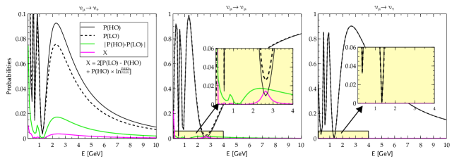
Figure 10: Similar to Fig. 8 but for contribution to explore the $\theta_{23}$-octant degeneracy.

References

- Cowan et al. (1956) C. Cowan, F. Reines, F. Harrison, H. Kruse, and A. McGuire, Science 124, 103 (1956).
- Pontecorvo (1957) B. Pontecorvo, Sov. Phys. JETP 6, 429 (1957).
- Pontecorvo (1958) B. Pontecorvo, Sov. Phys. JETP 7, 172 (1958).
- Maki et al. (1962) Z. Maki, M. Nakagawa, and S. Sakata, Progress of Theoretical Physics 28, 870 (1962).
- Gribov and Pontecorvo (1969) V. Gribov and B. Pontecorvo, Phys. Lett. B 28, 493 (1969).
- (6) T. Kajita and A. B. McDonald, the Nobel Prize in Physics 2015.https://www.nobelprize.org/prizes/physics/2015/summary/.
- Zyla et al. (2020) P. Zyla et al. (Particle Data Group), PTEP 2020, 083C01 (2020).
- Sakharov (1991) A. Sakharov, Sov. Phys. Usp. 34, 392 (1991).
- Fukugita and Yanagida (1986) M. Fukugita and T. Yanagida, Phys. Lett. B174, 45 (1986).
- Davidson et al. (2008) S. Davidson, E. Nardi, and Y. Nir, Phys. Rept. 466, 105 (2008), eprint 0802.2962.
- Branco et al. (2012) G. C. Branco, R. G. Felipe, and F. R. Joaquim, Rev. Mod. Phys. 84, 515 (2012), eprint 1111.5332.
- Petcov (1982) S. Petcov, Phys. Lett. B 110, 245 (1982).
- King et al. (2014) S. F. King, A. Merle, S. Morisi, Y. Shimizu, and M. Tanimoto, New J. Phys. 16, 045018 (2014), eprint 1402.4271.
- Haxton and Stephenson (1984) W. Haxton and G. Stephenson, Prog. Part. Nucl. Phys. 12, 409 (1984).
- Elliott and Engel (2004) S. R. Elliott and J. Engel, J. Phys. G 30, R183 (2004), eprint hep-ph/0405078.
- Aalseth et al. (2004) C. Aalseth et al. (2004), eprint hep-ph/0412300.
- Lam (2001) C. Lam, Phys. Lett. B 507, 214 (2001), eprint hep-ph/0104116.
- Harrison and Scott (2002) P. Harrison and W. Scott, Phys. Lett. B 547, 219 (2002), eprint hep-ph/0210197.
- Xing and Zhao (2016) Z.-z. Xing and Z.-h. Zhao, Rept. Prog. Phys. 79, 076201 (2016), eprint 1512.04207.
- Abe et al. (2014) K. Abe et al. (T2K), Phys. Rev. Lett. 112, 061802 (2014), eprint 1311.4750.
- Ayres et al. (2004) D. S. Ayres et al. (NOvA) (2004), eprint hep-ex/0503053.
- Abe et al. (2020) K. Abe et al. (T2K), Nature 580, 339 (2020), [Erratum: Nature 583, E16 (2020)], eprint 1910.03887.
- Acero et al. (2019) M. A. Acero et al. (NOvA), Phys. Rev. Lett. 123, 151803 (2019), eprint 1906.04907.
- de Salas et al. (2020) P. de Salas, D. Forero, S. Gariazzo, P. Martínez-Miravé, O. Mena, C. Ternes, M. Tórtola, and J. Valle (2020), eprint 2006.11237.
- Valencia-Globalfit (2020) Valencia-Globalfit, http://globalfit.astroparticles.es/ (2020).
- Capozzi et al. (2018) F. Capozzi, E. Lisi, A. Marrone, and A. Palazzo, Prog. Part. Nucl. Phys. 102, 48 (2018), eprint 1804.09678.
- Esteban et al. (2019) I. Esteban, M. C. Gonzalez-Garcia, A. Hernandez-Cabezudo, M. Maltoni, and T. Schwetz, JHEP 01, 106 (2019), eprint 1811.05487.
- Tórtola et al. (2020) M. A. Tórtola, G. A. Barenboim, and C. A. Ternes, JHEP 07, 155 (2020), eprint 2005.05975.
- Kelly et al. (2020) K. J. Kelly, P. A. Machado, S. J. Parke, Y. F. Perez Gonzalez, and R. Zukanovich-Funchal (2020), eprint 2007.08526.
- Acciarri et al. (2015) R. Acciarri et al. (DUNE) (2015), eprint 1512.06148.
- Abi et al. (2020a) B. Abi et al. (DUNE) (2020a), eprint 2002.03005.
- Abi et al. (2020b) B. Abi et al. (DUNE) (2020b), eprint 2006.16043.
- Masud et al. (2019a) M. Masud, M. Bishai, and P. Mehta, Sci. Rep. 9, 352 (2019a), eprint 1704.08650.
- Masud et al. (2019b) M. Masud, S. Roy, and P. Mehta, Phys. Rev. D 99, 115032 (2019b), eprint 1812.10290.
- De Gouvêa et al. (2019) A. De Gouvêa, K. J. Kelly, G. Stenico, and P. Pasquini, Phys. Rev. D 100, 016004 (2019), eprint 1904.07265.
- Ghoshal et al. (2019) A. Ghoshal, A. Giarnetti, and D. Meloni, JHEP 12, 126 (2019), eprint 1906.06212.
- Huber et al. (2009) P. Huber, M. Lindner, T. Schwetz, and W. Winter, JHEP 11, 044 (2009), eprint 0907.1896.
- Agarwalla et al. (2013) S. K. Agarwalla, S. Prakash, and S. Sankar, JHEP 07, 131 (2013), eprint 1301.2574.
- Machado et al. (2014) P. Machado, H. Minakata, H. Nunokawa, and R. Zukanovich Funchal, JHEP 05, 109 (2014), eprint 1307.3248.
- Ghosh et al. (2017) M. Ghosh, S. Goswami, and S. K. Raut, Mod. Phys. Lett. A 32, 1750034 (2017), eprint 1409.5046.
- Ghosh et al. (2016a) M. Ghosh, P. Ghoshal, S. Goswami, N. Nath, and S. K. Raut, Phys. Rev. D 93, 013013 (2016a), eprint 1504.06283.
- Ghosh et al. (2016b) M. Ghosh, S. Goswami, and S. K. Raut, Eur. Phys. J. C 76, 114 (2016b), eprint 1412.1744.
- Nath et al. (2016) N. Nath, M. Ghosh, and S. Goswami, Nucl. Phys. B 913, 381 (2016), eprint 1511.07496.
- Coloma et al. (2014) P. Coloma, H. Minakata, and S. J. Parke, Phys. Rev. D 90, 093003 (2014), eprint 1406.2551.
- Adams et al. (2013) C. Adams et al. (LBNE), in Snowmass 2013: Workshop on Energy Frontier (2013), eprint 1307.7335.
- Ballett et al. (2017) P. Ballett, S. F. King, S. Pascoli, N. W. Prouse, and T. Wang, Phys. Rev. D 96, 033003 (2017), eprint 1612.07275.
- (47) DUNE Internal Document DUNE-doc-20412-v1.
- Huber et al. (2005) P. Huber, M. Lindner, and W. Winter, Comput. Phys. Commun. 167, 195 (2005), eprint hep-ph/0407333.
- Huber et al. (2007) P. Huber, J. Kopp, M. Lindner, M. Rolinec, and W. Winter, Comput. Phys. Commun. 177, 432 (2007), eprint hep-ph/0701187.
- Dziewonski and Anderson (1981) A. M. Dziewonski and D. L. Anderson, Phys. Earth Planet. Interiors 25, 297 (1981).
- Gandhi et al. (2005) R. Gandhi, P. Ghoshal, S. Goswami, P. Mehta, and S. U. Sankar, Phys.Rev.Lett. 94, 051801 (2005), eprint hep-ph/0408361.
- Gandhi et al. (2006) R. Gandhi, P. Ghoshal, S. Goswami, P. Mehta, and S. U. Sankar, Phys.Rev. D73, 053001 (2006), eprint hep-ph/0411252.
- Kelly and Parke (2018) K. J. Kelly and S. J. Parke, Phys. Rev. D 98, 015025 (2018), eprint 1802.06784.
- Chatterjee et al. (2018) A. Chatterjee, F. Kamiya, C. A. Moura, and J. Yu (2018), eprint 1809.09313.
- Alion et al. (2016) T. Alion et al. (DUNE) (2016), eprint 1606.09550.
- Agostinelli et al. (2003) S. Agostinelli et al. (GEANT4), Nucl. Instrum. Meth. A506, 250 (2003).
- Allison et al. (2006) J. Allison et al., IEEE Trans. Nucl. Sci. 53, 270 (2006).
- Huber et al. (2002) P. Huber, M. Lindner, and W. Winter, Nucl. Phys. B645, 3 (2002), eprint hep-ph/0204352.
- Fogli et al. (2002) G. L. Fogli, E. Lisi, A. Marrone, D. Montanino, and A. Palazzo, Phys. Rev. D66, 053010 (2002), eprint hep-ph/0206162.
- Gonzalez-Garcia and Maltoni (2004) M. Gonzalez-Garcia and M. Maltoni, Phys.Rev. D70, 033010 (2004), eprint hep-ph/0404085.
- Gandhi et al. (2007) R. Gandhi, P. Ghoshal, S. Goswami, P. Mehta, S. U. Sankar, and S. Shalgar, Phys. Rev. D76, 073012 (2007), eprint 0707.1723.
- Qian et al. (2012) X. Qian, A. Tan, W. Wang, J. J. Ling, R. D. McKeown, and C. Zhang, Phys. Rev. D86, 113011 (2012), eprint 1210.3651.
- Masud et al. (2016) M. Masud, A. Chatterjee, and P. Mehta, J. Phys. G43, 095005 (2016), eprint 1510.08261.
- Masud and Mehta (2016a) M. Masud and P. Mehta, Phys. Rev. D94, 013014 (2016a), eprint 1603.01380.
- Masud and Mehta (2016b) M. Masud and P. Mehta, Phys. Rev. D94, 053007 (2016b), eprint 1606.05662.