Nikhef/2020-022

Exploiting the information provided by electron energy-loss spectroscopy (EELS) requires reliable access to the low-loss region where the zero-loss peak (ZLP) often overwhelms the contributions associated to inelastic scatterings off the specimen. Here we deploy machine learning techniques developed in particle physics to realise a model-independent, multidimensional determination of the ZLP with a faithful uncertainty estimate. This novel method is then applied to subtract the ZLP for EEL spectra acquired in flower-like WS₂ nanostructures characterised by a 2H/3R mixed polytypism. From the resulting subtracted spectra we determine the nature and value of the bandgap of polytypic WS₂, finding $E_{\rm BG}=1.6_{-0.2}^{+0.3}\,{\rm eV}$ with a clear preference for an indirect bandgap. Further, we demonstrate how this method enables us to robustly identify excitonic transitions down to very small energy losses. Our approach has been implemented and made available in an open source Python package dubbed EELSfitter.

Keywords: Transmission Electron Microscopy, Electron Energy Loss Spectroscopy, Neural Networks, Machine Learning, Transition Metal Dichalcogenides, Bandgap.

^∗corresponding author: s.conesaboj@tudelft.nl

1 Introduction

Electron energy-loss spectroscopy (EELS) within the transmission electron microscope (TEM) provides a wide range of valuable information on the structural, chemical, and electronic properties of nanoscale materials. Thanks to recent instrumentation breakthroughs such as electron monochromators [1, 2] and aberration correctors [3], modern EELS analyses can study these properties with highly competitive spatial and spectral resolution. A particularly important region of EEL spectra is the low-loss region, defined by electrons that have lost a few tens of eV, $\Delta E\mathrel{\hbox to0.0pt{\lower 4.0pt\hbox{\hskip 1.0pt$\sim$}\hss}\raise 1.0pt\hbox{$<$}}50$ eV, following their inelastic interactions with the sample. The analysis of this low-loss region makes possible charting the local electronic properties of nanomaterials [4], from the characterisation of bulk and surface plasmons [5], excitons [6], inter- and intra-band transitions [7], and phonons to the determination of their bandgap and band structure [8].

Provided the specimen is electron-transparent, as required for TEM inspection, the bulk of the incident electron beam will traverse it either without interacting or restricted to elastic scatterings with the atoms of the sample’s crystalline lattice. In EEL spectra, these electrons are recorded as a narrow, high intensity peak centered at energy losses of $\Delta E\simeq 0$, known as the zero-loss peak (ZLP). The energy resolution of EELS analyses is ultimately determined by the electron beam size of the system, often expressed in terms of the full width at half maximum (FWHM) of the ZLP [9]. In the low-loss region, the contribution from the ZLP often overwhelms that from the inelastic scatterings arising from the interactions of the beam electrons with the sample. Therefore, relevant signals of low-loss phenomena such as excitons, phonons, and intraband transitions risk becoming drowned in the ZLP tail [10]. An accurate removal of the ZLP contribution is thus crucial in order to accurately chart and identify the features of the low-loss region in EEL spectra.

In monochromated EELS, the properties of the ZLP depend on the electron energy dispersion, the monochromator alignment, and the sample thickness [11, 8]. The first two factors arise already in the absence of a specimen (vacuum operation), while the third is associated to interactions with the sample such as atomic scatterings, phonon excitation, and exciton losses. This implies that EEL measurements in vacuum can be used for calibration purposes but not to subtract the ZLP from spectra taken on specimens, since their shapes will in general differ.

Several approaches to ZLP subtraction[12, 8, 13] have been put forward in the literature. These are often based on specific model assumptions about the ZLP properties, in particular concerning its parametric functional dependence on the electron energy loss $\Delta E$, from Lorentzian [14] and power laws [6] to more general multiple-parameter functions [15]. Another approach is based on mirroring the $\Delta E<0$ region of the spectra, assuming that the $\Delta E>0$ region is fully symmetric [16]. More recent studies use integrated software applications for background subtraction [17, 18, 19, 20]. These various methods are however affected by three main limitations. Firstly, their reliance on model assumptions such as the choice of fit function introduces a methodological bias whose size is difficult to quantify. Secondly, they lack an estimate of the associated uncertainties, which in turn affects the reliability of any physical interpretations of the low loss region. Thirdly, ad hoc choices such as those of the fitting ranges introduce a significant degree of arbitrariness in the procedure.

In this study we bypass these limitations by developing a model-independent strategy to realise a multidimensional determination of the ZLP with a faithful uncertainty estimate. Our approach is based on machine learning (ML) techniques originally developed in high-energy physics to study the quark and gluon substructure of protons in particle collisions [21, 22, 23, 24]. It is based on the Monte Carlo replica method to construct a probability distribution in the space of experimental data and artificial neural networks as unbiased interpolators to parametrise the ZLP. The end result is a faithful sampling of the probability distribution in the ZLP space which can be used to subtract its contribution to EEL spectra while propagating the associated uncertainties. One can also extrapolate the predictions from this ZLP parametrisation to other TEM operating conditions beyond those included in the training dataset.

This work is divided into two main parts. In the first one, we construct a ML model of ZLP spectra acquired in vacuum, which is able to accommodate an arbitrary number of input variables corresponding to different operation settings of the TEM. We demonstrate how this model successfully describes the input spectra and we assess its extrapolation capabilities for other operation conditions. In the second part, we construct a one-dimensional model of the ZLP as a function of $\Delta E$ from spectra acquired on two different specimens of tungsten disulfide (WS₂) nanoflowers characterised by a 2H/3R mixed polytypism [25]. The resulting subtracted spectra are used to determine the value and nature of the WS₂ bandgap in these nanostructures as well as to map the properties of the associated exciton peaks appearing in the ultra-low loss region.

This paper is organized as follows. First of all, in Sect. 2 we review the main features of EELS and present the WS₂ nanostructures that will be used as proof of concept of our approach. In Sect. 3 we describe the machine learning methodology adopted to model the ZLP features. Sects. 4 and 5 contain the results of the ZLP parametrisation of spectra acquired in vacuum and in specimens respectively, which in the latter case allows us to probe the local electronic properties of the WS₂ nanoflowers. Finally in Sect. 6 we summarise and outline possible future developments. Our results have been obtained with an open-source Python code, dubbed EELSfitter, whose installation and usage instructions are described in Appendix A.

2 EELS analyses and TMD nanostructures

In this work, we will apply our machine learning method to the study of the low-loss EELS region of a specific type of WS₂ nanostructures presented in [25], characterised by a flower-like morphology and a 2H/3R mixed polytypism. WS₂ is a member of the transition metal dichalcogenide (TMD) family, which in turn belongs to a class of materials known as two-dimensional, van der Waals, or simply layered materials. These materials are characterised by the remarkable property of being fully functional down to a single atomic layer. In order to render the present work self-contained and accessible to a wider audience, here we review the basic concepts underlying the EELS technique, and then present the main features of the WS₂ nanoflowers that will be studied in the subsequent sections.

2.1 EELS and its ZLP in a nutshell

Electron energy loss spectroscopy is a TEM-based method whereby an electron-transparent sample is illuminated by a beam of energetic electrons. Subsequent to the crossing of the specimen, the scattered electron beam is focused by a magnetic prism towards a spectrometer where the distribution of electron energy losses $\Delta E$ can be recorded. The schematic illustration of a typical EELS setup is shown in the left panel of Fig. 2.1. EEL spectra can be recorded either in the Scanning Transmission Electron Microscopy (STEM) mode or in the conventional TEM (c-TEM) setup. Thanks to recent progress in TEM instrumentation and data acquisition, state-of-the-art EELS analyses benefit from a highly competitive energy (spectral) resolution combined with an unparalleled spatial resolution.

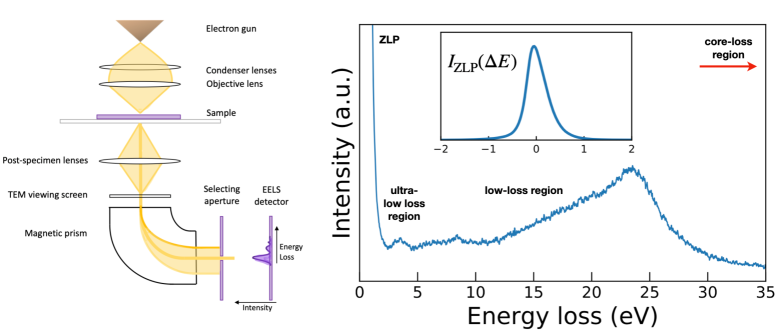
Figure 2.1: Left: schematic representation of the STEM-EELS setup. A magnetic prism is used to deflect the electron beam after it has crossed the sample, allowing the distribution of energy losses $\Delta E$ to be recorded with a spectrometer. Right: a representative low-loss EEL spectrum acquired on a WS₂ nanoflower [25] with the inset displaying the corresponding ZLP.

EELS spectra can be approximately divided into three main regions. The first is the zero-loss region, centered around $\Delta E=0$ and containing the contributions from both elastic scatterings as well as those from electrons that have not interacted with the sample. This region is characterised by the strong and narrow ZLP which dominates over the contribution from inelastic scatterings. The second region is the low-loss region, defined for energy losses $\Delta E\mathrel{\hbox to0.0pt{\lower 4.0pt\hbox{\hskip 1.0pt$\sim$}\hss}\raise 1.0pt\hbox{$<$}}50$ eV, which contains information about several important features such as plasmons, excitons, phonons, and intra-band transitions. Of particular relevance in this context is the ultra-low loss region, characterised by $\Delta E\simeq$ few eV. There, the contributions of the ZLP and those from inelastic interactions become comparable. The regime for which $\Delta E\mathrel{\hbox to0.0pt{\lower 4.0pt\hbox{\hskip 1.0pt$\sim$}\hss}\raise 1.0pt\hbox{$>$}}50$ eV is then known as the core-loss region and provides compositional information on the materials that constitute the specimen.

The right panel of Fig. 2.1 displays a representative EELS spectrum in the region $\Delta E\leq 35$ eV, recorded in one of the WS₂ nanoflowers of [25]. The inset displays the ZLP, illustrating how nearby $\Delta E\simeq 0$ its size is larger than the contribution from the inelastic scatterings off the sample by several orders of magnitude. Carefully disentangling these two contributions is essential for the physical interpretation of EEL spectra in the ultra-low-loss region.

The magnitude and shape of the ZLP intensity is known to depend not only on the specific values of the electron energy loss $\Delta E$, but also on other operation parameters of the TEM such as the electron beam energy $E_{b}$, the exposure time $t_{\rm exp}$, the aperture width, and the use of a monochromator. Since it is not possible to compute the dependence of the ZLP on $\Delta E$ and the other operation parameters from first principles, reliance on specific models seems to be unavoidable. This implies that one cannot measure the ZLP for a given operating condition, for instance a high beam voltage of 200 kV, and expect to reproduce the ZLP intensity distribution associated to different conditions, such as a lower beam voltage of 60 kV, without introducing model assumptions.

Several attempts to describe the ZLP distribution have reported some success at predicting the main intensity of the peak, but in the tails discrepancies are as large as several tens of percent [26]. The standard method for background subtraction is to fit a power law to the tails, however this approach is not suitable in many circumstances [27, 28, 29, 30]. Further, even for nominally identical operating conditions, the intensity of the ZLP will in general vary due to e.g. external perturbations such as electric or magnetic fields [12], the stability of the microscope and spectrometer electronics [31], the local environment (possibly exposed to mechanical, pressure and temperature fluctuations) and spectral aberrations [13]. Any robust statistical model for the ZLP should thus account for this irreducible source of uncertainties.

2.2 TMD materials and WS₂ nanoflowers

In this work we will apply our ZLP parametrisation strategy to a novel class of recently presented WS₂ nanostructures known as nanoflowers [25]. WS₂ belongs to the TMD class of layered materials together with e.g. MoS₂ and WSe₂. TMD materials are of the form MX₂, where M is a transition metal atom (such as Mo or W) and X a chalcogen atom (such as S, Se, or Te). The characteristic crystalline structure of TMDs is such that one layer of M atoms is sandwiched between two layers of X atoms.

The local electronic structure of TMDs strongly depends on the coordination between the transition metal atoms, giving rise to an array of remarkable electronic and magnetic properties [32]. Furthermore, the properties of this class of materials vary significantly with their thickness, for instance MoS₂ exhibits an indirect bandgap in the bulk form which becomes direct at the monolayer level [33]. The tunability of their electronic properties and the associated potential applications in nano-electronics make TMD materials highly attractive for fundamental research.

As for other TMD materials, WS₂ adopts a layered structure by stacking atomic layers of S-W-S in a sandwich-like configuration. Although the interaction between adjacent layers is a weak Van der Waals force, the dependence of the interlayer interactions on the stacking order of WS₂ can be significant. Therefore, modulating the stacking arrangement of WS₂ layers (as well as their relative orientation) represents a promising handle to tailor the resulting local electronic properties. WS₂ also exhibits a marked thickness dependence of its properties, with an indirect-to-direct bandgap transition when going from bulk to bilayer or monolayer form. The effects of this transition are manifested for example as enhanced photoluminescence in monolayer WS₂, whereas greatly suppressed emission is observed in the corresponding bulk form [34]. Further applications of this material include storage of hydrogen and lithium for batteries [35].

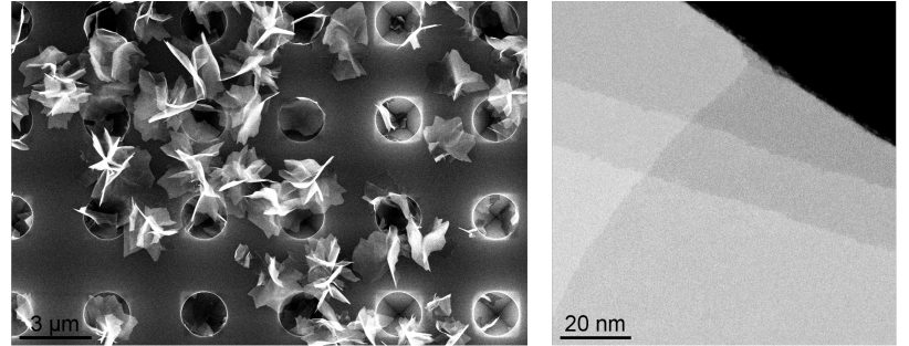
Figure 2.2: Left: low-magnification TEM image of the WS₂ nanoflowers grown on top of a holey Si/SiN substrate. Right: the magnification of a representative petal of a nanoflower, where the black region corresponds to the vacuum (no substrate) and the difference in contrast indicates terraces of varying thickness.

A low-magnification TEM image of the WS₂ nanoflowers is displayed in the left panel of Fig. 2.2. These nanostructures are grown directly on top of a holey TEM substrate. The right panel shows the magnification of a representative petal of a nanoflower, where the difference in contrast indicates terraces of varying thickness. Note that the black region corresponds to the vacuum, that is, without substrate underneath. These WS₂ nanoflowers exhibit a wide variety of thicknesses, orientations and crystalline structures, therefore representing an ideal laboratory to correlate structural morphology in WS₂ with electronic properties at the nanoscale. Importantly, these nanoflowers are characterised by a mixed crystalline structure, in particular 2H/3R polytypism. This implies that different stacking types tend to coexist, affecting the interlayer interactions within WS₂ and thus modifying the resulting physical properties [36]. One specific consequence of such variations in the stacking patterns is the appearance of spontaneous electrical polarization, leading to modifications of the electronic band structure and thus of the bandgap [37, 38].

As mentioned above, one of the most interesting properties of WS₂ is that when the material is thinned down to a single monolayer its indirect bandgap of $E_{\rm BG}\simeq 1.4$ eV switches to a direct bandgap of approximately $E_{\rm BG}\simeq 2.1$ eV. It has been found that the type and magnitude of the WS₂ bandgap depends quite sensitively on the crystalline structure and the number of layers that constitute the material. In Table 2.1 we collect representative results for the determination of the bandgap energy $E_{\rm BG}$ and its type in WS₂, obtained by means of different experimental and theoretical techniques. For each reference we indicate separately the bulk results and those obtained at the monolayer level. We note that for the latter case there is a fair spread of results in the value of $E_{\rm BG}$, reflecting the challenges of its accurate determination.

Reference	Thickness	$E_{\rm BG}$ (eV)	bandgap type	Technique
[39]	bulk	$1.4\pm 0.07$	indirect	Gate-voltage dependence
[40]	monolayer	$2.14$	direct	Gate-voltage dependence
	bulk	$1.40$	indirect
[41]	monolayer	$2.03\pm 0.03$	direct	Density Functional Theory
	bulk	$1.32\pm 0.03$	indirect
[42]	monolayer	$1.76\pm 0.03$	direct	Absorption edge coefficient fitting
	bulk	$1.35$	indirect
[43]	monolayer	$2.21\pm 0.3$	direct	Bethe-Salpeter equation (BSE)

Table 2.1: Representative results for the determination of the bandgap energy $E_{\rm BG}$ and its type in WS₂, obtained by means of different experimental and theoretical techniques. For each reference we indicate separately the bulk results and those obtained at the monolayer level.

3 A neural network determination of the ZLP

In this section we present our strategy to parametrise and subtract in a model-independent manner the zero-loss peak that arises in the low-loss region of EEL spectra by means of machine learning. As already mentioned, our strategy follows the NNPDF approach [44] originally developed in the context of high-energy physics for studies of the quark and gluon substructure of the proton [45]. The NNPDF approach has been successfully applied, among others, to the determination of the unpolarised [46, 21, 22, 23, 24] and polarised [47] parton distribution functions of protons, nuclear parton distributions [48, 49], and the fragmentation functions of partons into neutral and charged hadrons [50, 51].

We note that recently several applications of machine learning to transmission electron microscopy analyses in the context of material science have been presented, see e.g. [52, 53, 54, 55, 56, 57, 58]. Representative examples include the automated identification of atomic-level structural information [56], the extraction of chemical information and defect classification [57], and spatial resolution enhancement by means of generative adversarial networks [58]. To the best of our knowledge, this is the first time that neural networks are used as unbiased background-removal interpolators and combined with Monte Carlo sampling to construct a faithful estimate of the model uncertainties.

In this section first of all we discuss the parametrisation of the ZLP in terms of neural networks. We then review the Monte Carlo replica method used to estimate and propagate the uncertainties from the input data to physical predictions. Subsequently, we present our training strategy both in case of vacuum and of sample spectra, and discuss how one can select the optimal values of the hyper-parameters that appear in the model.

3.1 ZLP parametrisation

To begin with we note that, without any loss of generality, the intensity profile associated to a generic EEL spectrum may be decomposed as

$$I_{\rm EEL}(\Delta E)=I_{\rm ZLP}(\Delta E)+I_{\rm inel}(\Delta E)\,,$$ (3.1)

where $\Delta E$ is the measured electron energy loss; $I_{\rm ZLP}$ is the zero-loss peak distribution arising both from instrumental origin and from elastic scatterings; and $I_{\rm inel}(\Delta E)$ contains the contributions from the inelastic scatterings off the electrons and atoms in the specimen. As illustrated by the representative example of Fig. 2.1, there are two limits for which one can cleanly disentangle the two contributions. First of all, for large enough values of $\Delta E$ then $I_{\rm ZLP}$ vanishes and thus $I_{\rm EEL}\to I_{\rm inel}$. Secondly, in the $\Delta E\simeq 0$ limit all emission can be associated to the ZLP such that $I_{\rm EEL}\to I_{\rm ZLP}$. In this work we are interested in the ultra-low-loss region, where $I_{\rm ZLP}$ and $I_{\rm inel}$ become of the comparable magnitude.

Our goal is to construct a parametrisation of $I_{\rm ZLP}$ based on artificial neural networks, which we denote by $I_{\rm ZLP}^{\rm(mod)}$, by means of which one can extract the inelastic contributions by subtracting the ZLP background model to the measured intensity spectra,

$$I_{\rm inel}(\Delta E)\simeq I_{\rm EEL}(\Delta E)-I_{\rm ZLP}^{\rm(mod)}(\Delta E)\,,$$ (3.2)

which enables us to exploit the physical information contained in $I_{\rm inel}$ in the low-loss region. Crucially, we aim to faithfully estimate and propagate all the relevant sources of uncertainty associated both to the input data and to methodological choices.

As discussed in Sect. 2.1, the ZLP depends both on the value of the electron energy loss $\Delta E$ as well as on the operation parameters of the microscope, such as the electron beam energy $E_{b}$ and the exposure time $t_{\rm exp}$. Therefore, we want to construct a multidimensional model which takes all relevant variables as input. This means that in general Eq. (3.2) must be written as

$$I_{\rm inel}(\Delta E)\simeq I_{\rm EEL}(\Delta E,E_{b},t_{\rm exp},\ldots)-I_{\rm ZLP}^{\rm(mod)}(\Delta E,E_{b},t_{\rm exp},\ldots)\,,$$ (3.3)

where we note that the subtracted spectra should depend only on $\Delta E$ but not on the microscope operation parameters. Ideally, the ZLP model should be able to accomodate as many input variables as possible. Here we parametrise $I_{\rm ZLP}^{\rm(mod)}$ by means of multi-layer feed-forward artificial neural networks [59], that is, we express our ZLP model as

$$I_{\rm ZLP}^{\rm(mod)}(\Delta E,E_{b},t_{\rm exp},\ldots)=\xi^{(n_{l})}_{1}(\Delta E,E_{b},t_{\rm exp},\ldots)\,,$$ (3.4)

where $\xi^{(n_{l})}_{1}$ denotes the activation state of the single neuron in the last of the $n_{l}$ layers of the network when the $n_{I}$ inputs $\{\Delta E,E_{b},t_{\rm exp},\ldots\}$ are used. The weights and thresholds $\{\omega_{ij}^{(l)},\theta_{i}^{(l)}\}$ of this neural network model are then determined from the maximization of the model likelihood by means of supervised learning and non-linear regression from a suitable training dataset. This type of neural networks benefit from the ability to parametrise multidimensional input data with arbitrarily non-linear dependencies: even with a single hidden layer, a neural network can reproduce arbitrary functional dependencies provided it has a large enough number of neurons.

A schematic representation of our model is displayed in Fig. 3.1. The input is an $n_{I}$ array containing $\Delta E$ and the rest of operation variables of the microscope, and the output is the value of the intensity of the ZLP distribution associated to those input variables. We adopt an $n_{I}$-10-15-5-1 architecture with three hidden layers, for a total number of 289 (271) free parameters for $n_{I}=3$ ($n_{I}=1$) to be adjusted by the optimization procedure. We use a sigmoid activation function for the three hidden layers and a ReLU for the final one. The choice of ReLU for the final layer guarantees that our model for the ZLP is positive-definite, as required by general physical considerations. We have adopted a redundant architecture to ensure that the ZLP parametrisation is sufficiently flexible, and we avoid over-fitting by means of a suitable regularisation strategy described in Sect. 3.3.

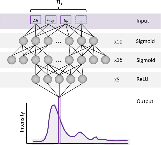
Figure 3.1: Schematic representation of our neural network model for the ZLP, Eq. (3.4). The input is an $n_{I}$-dimensional array containing $\Delta E$ and other operation variables of the microscope such as $E_{b}$ and $t_{\rm exp}$. The output is the predicted value of the intensity of the zero-loss peak distribution associated to those specific input variables. The architecture is chosen to be $n_{I}$-10-15-5-1, with sigmoid activation functions in all layers except for a ReLU in the output neuron.

3.2 Uncertainty propagation

We discussed in Sect. 2.1 how even for EEL spectra taken at nominally identical operation conditions of the microscope, in general the resulting ZLP intensities will differ. Further, there exist a large number of different NN configurations, each representing a different functional form for $I_{\rm ZLP}^{(\rm mod)}$ which provide an equally valid description of the input data. To estimate these uncertainties and propagate them to physical predictions, we use here the Monte Carlo replica method. The basic idea is to exploit the available information on experimental measurements (central values, uncertainties, and correlations) to construct a sampling of the probability density in the space of the data, which by means of the NN training is then propagated to a probability density in the space of $I_{\rm ZLP}$ models.

Let us assume that we have $n_{\rm dat}$ independent measurements of the ZLP intensity, for different or the same values of the input parameters collectively denoted as $\{z_{i}\}$:

$$I^{\rm(exp)}_{{\rm ZLP},i}\left(\{z_{i}\}\right)=I^{\rm(exp)}_{{\rm ZLP},i}\left(\Delta E_{i},E_{b,i},t_{{\rm exp},i},\ldots\right)\,,\quad i=1,\ldots,n_{\rm dat}\,.$$ (3.5)

From these measurements, we can generate a large sample of artificial data points that will be used as training inputs for the neural nets by means of the Monte Carlo replica method. In such approach, one generates $N_{\rm rep}$ Monte Carlo replicas of the original data points by means of a multi-Gaussian distribution, with the central values and covariance matrices taken from the input measurements,

$$I_{{\rm ZLP},i}^{{\rm(art)}(k)}=I^{\rm(exp)}_{{\rm ZLP},i}+r_{i}^{({\rm stat},k)}\sigma_{i}^{\rm(stat)}+\sum_{j=1}^{n_{\rm sys}}r_{i,j}^{({\rm sys},k)}\sigma_{i,j}^{\rm(\rm sys)}\,,\quad\forall i\,,\quad k=1,\ldots,N_{\rm rep}\,,\,\,\,$$ (3.6)

where $\sigma_{i}^{\rm(stat)}$ and $\sigma_{i,j}^{\rm(\rm sys)}$ represent the statistical and systematic uncertainties (the latter divided into $n_{\rm sys}$ fully point-to-point correlated sources) and $\{r_{i}^{(k)}\}$ are Gaussianly distributed random numbers. The values of $\{r_{i}^{(k)}\}$ are generated with a suitable correlation pattern to ensure that averages over the set of Monte Carlo replicas reproduce the original experimental covariance matrix, namely

$$\left\langle\left(I_{{\rm ZLP},i}^{{\rm(art)}(k)}-\left\langle I_{{\rm ZLP},i}^{{\rm(art)}}\right\rangle_{\rm rep}\right)\left(I_{{\rm ZLP},j}^{{\rm(art)}(k)}-\left\langle I_{{\rm ZLP},j}^{{\rm(art)}}\right\rangle_{\rm rep}\right)\right\rangle_{\rm rep}={\rm cov}^{(\rm exp)}\left(I_{{\rm ZLP},i},I_{{\rm ZLP},j}\right)\,,$$ (3.7)

where averages are evaluated over the $N_{\rm rep}$ replicas that compose the sample. We thus note that each $k$-th replica contains as many data points as the original set.

In our case, the information on experimental correlations is not accessible and thus we assume that there is a single source of point-by-point uncorrelated systematic uncertainty, denoted as $\sigma_{i}^{\rm(exp)}$, which is estimated as follows. The input measurements will be composed in general on subsets of EEL spectra taken with identical operation conditions. Assume that for a specific set of operation conditions we have $N_{\rm sp}$ of such spectra. Since the values of $\Delta E$ will be different in each case, first of all we uniformise a common binning in $\Delta E$ with $n_{\rm dat}$ entries. Then we evaluate the total experimental uncertainty in one of these bins as

$$\sigma_{i}^{\rm(exp)}=\left({{1}\over{N_{\rm sp}-1}}\sum_{l=1}^{N_{\rm sp}}\left(I_{{\rm ZLP},i}^{({\rm exp}),l}-\left\langle I_{{\rm ZLP},i}^{({\rm exp})}\right\rangle_{N_{\rm sp}}\right)\right)^{1/2}\,,\,i=1,\ldots,n_{\rm dat}\,,$$ (3.8)

that is, as the standard deviation over the $N_{\rm sp}$ spectra. This uncertainty is separately evaluated for each set of microscope operation conditions for which data available. In the absence of correlations, Eqns. (3.6) and (3.7) simplify to

$$I_{{\rm ZLP},i}^{{\rm(art)}(k)}=I^{\rm(exp)}_{{\rm ZLP},i}+r_{i}^{({\rm tot},k)}\sigma_{i}^{\rm(exp)}\,,\quad\forall i\,,\quad k=1,\ldots,N_{\rm rep}\,.\,\,\,$$ (3.9)

and

$$\left\langle\left(I_{{\rm ZLP},i}^{{\rm(art)}(k)}-\left\langle I_{{\rm ZLP},i}^{{\rm(art)}}\right\rangle_{\rm rep}\right)\left(I_{{\rm ZLP},j}^{{\rm(art)}(k)}-\left\langle I_{{\rm ZLP},j}^{{\rm(art)}}\right\rangle_{\mathrm{rep}}\right)\right\rangle_{\rm rep}=\sigma_{i}^{\rm(exp)}\sigma_{j}^{\rm(exp)}\delta_{ij}\,,$$ (3.10)

since the experimental covariance matrix is now diagonal. Should in the future correlations became available, it would be straightforward to extend our model to that case.

The value of the number of generated MC replicas, $N_{\rm rep}$, should be chosen such that the set of replicas accurately reproduces the probability distribution of the original training data. To verify that this is the case, Fig. 3.2 displays a comparison between the original experimental central values $I_{{\rm ZLP},i}^{\rm(exp)}$ and the corresponding total uncertainties $\sigma_{i}^{(\rm exp)}$ with the results of averaging over a sample of $N_{\rm rep}$ Monte Carlo replicas generated by means of Eq. (3.6) for different number of replicas. We find that $N_{\rm rep}=500$ is a value that ensures that both the central values and uncertainties are reasonably well reproduced, and we adopt it in what follows.

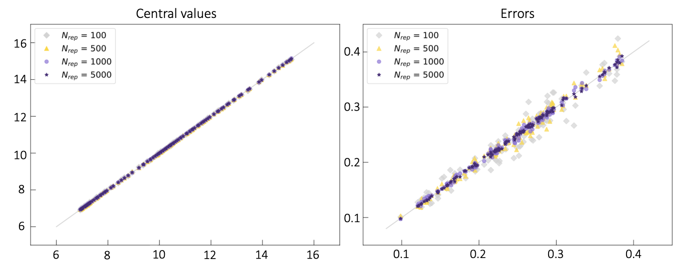
Figure 3.2: Comparison between the original experimental central values $I_{\rm ZLP,i}^{\rm(exp)}$ (left) and the corresponding uncertainties $\sigma_{i}^{(\rm exp)}$ (right panel) with the results of averaging over a sample of $N_{\rm rep}$ Monte Carlo replicas generated by means of Eq. (3.6), for different values of $N_{\rm rep}$.

3.3 Training strategy

The training of the neural network model for the ZLP peak differs between the cases of EEL spectra taken on vacuum, where by construction $I_{\rm EEL}(\Delta E)=I_{\rm ZLP}^{\rm(mod)}(\Delta E)$, and for spectra taken on specimens. In the latter case, as indicated by Eq. (3.2), in order to avoid biasing the results it is important to ensure that the model is trained only on the region of the spectra where the ZLP dominates over the inelastic scatterings. We now describe the training strategy that is adopted for these two cases.

Training on vacuum spectra.

For each of the $N_{\rm rep}$ generated Monte Carlo replicas, we train an independent neural network as described in Sect. 3.1. The parameters of the neural network $\{\theta^{(k)}\}$ (its weights and thresholds) are determined from the minimisation of a figure of merit (the cost function of the model) defined as

$$\centering E^{(k)}\left(\{\theta^{(k)}\}\right)={{1}\over{n_{\rm dat}}}\sum_{i=1}^{n_{\rm dat}}\left({{I_{{\rm ZLP},i}^{{\rm(art)}(k)}-I_{{\rm ZLP},i}^{{\rm(mod)}}\left(\{\theta^{(k)}\}\right)}\over{\sigma_{i}^{(\rm exp)}}}\right)^{2},\@add@centering$$ (3.11)

which is the $\chi^{2}$ per data point obtained by comparing the $k$-th replica for the ZLP intensity with the corresponding model prediction for the values $\{\theta^{(k)}\}$ of its weights and thresholds. In order to speed up the neural network training process, prior to the optimisation all inputs and outputs are scaled to lie between $[0.1,0.9]$ before being fed to the network. This preprocessing facilitates that the neuron activation states will typically lie close to the linear region of the sigmoid activation function.

The contribution to the figure of merit from the input experimental data, Eq. (3.11), needs in general to be complemented with that of theoretical constraints on the model. For instance, when determining nuclear parton distributions [49], one needs to extend Eq. (3.11) with Lagrange multipliers to ensure that both the $A=1$ proton boundary condition and the cross-section positivity are satisfied. In the case at hand, our model for the ZLP should implement the property that $I_{\rm ZLP}(\Delta E)\to 0$ when $|\Delta E|\to\infty$, since far from $\Delta E\simeq 0$ the contribution from elastic scatterings and instrumental broadening is completely negligible. In order to implement this constraint, we add $n_{\rm pd}$ pseudo-data points to the training dataset and modify the figure of merit Eq. (3.11) as follows

$$E^{(k)}\left(\{\theta^{(k)}\}\right)\to E^{(k)}\left(\{\theta^{(k)}\}\right)+\lambda\sum_{i^{\prime}=1}^{n_{\rm pd}}\left(I_{{\rm ZLP},i^{\prime}}^{{\rm(mod)}}\left(\{\theta^{(k)}\}\right)\right)^{2},$$ (3.12)

where $\lambda$ is a Lagrange multiplier whose value is tuned to ensure that the $I_{\rm ZLP}(\Delta E)\to 0$ condition is satisfied without affecting the description of the training dataset. The pseudo-data is chosen to lie in the region $[\Delta E_{\rm pd}^{\rm(min)},\Delta E_{\rm pd}^{\rm(max)}]$ (and symmetrically for energy gains).

The value of $\Delta E_{\rm pd}^{\rm(min)}$ can be determined automatically by evaluating the ratio $\mathcal{R}_{\rm sig}$ between the central experimental intensity and the total uncertainty in each data point,

$$\mathcal{R}_{\rm sig}(\Delta E_{i})\equiv{{I_{{\rm ZLP}}^{(\rm exp)}(\Delta E_{i})}\over{\sigma^{(\rm exp)}(\Delta E_{i})}}\,,$$ (3.13)

which corresponds to the statistical significance for the $i$-th bin of $\Delta E$ to differ from the null hypothesis (zero intensity) taking into account the experimental uncertainties. For sufficiently large energy losses one finds that $\mathcal{R}_{\rm sig}(\Delta E)\mathrel{\hbox to0.0pt{\lower 4.0pt\hbox{\hskip 1.0pt$\sim$}\hss}\raise 1.0pt\hbox{$<$}}1$, indicating that one would be essentially fitting statistical noise. In order to avoid such a situation and only fit data that is different from zero within errors, we determine $\Delta E_{\rm pd}^{\rm(min)}$ from the condition $\mathcal{R}_{\rm sig}\simeq 1$. We then maintain the training data in the region $\Delta E\leq\Delta E_{\rm pd}^{\rm(min)}$ and the pseudo-data points are added for $[\Delta E_{\rm pd}^{\rm(min)},\Delta E_{\rm pd}^{\rm(max)}]$. The value of $\Delta E_{\rm pd}^{\rm(max)}$ can be chosen arbitrarily and can be as large as necessary to ensure that $I_{\rm ZLP}(\Delta E)\to 0$ as $|\Delta E|\to\infty$.

We note that another important physical condition on the ZLP model, namely its positivity (since in EEL spectra the intensity is just a measure of the number of counts in the detector for a given value of the energy loss), is automatically satisfied given that we adopt a ReLU activation function for the last layer.

In this work we adopt the TensorFlow library [60] to assemble the architecture illustrated in Fig. 3.1. Before training, all weights and biases are initialized in a non-deterministic order by the built-in global variable initializer. The optimisation of the figure of merit Eq. (3.12) is carried out by means of stochastic gradient descent (SGD) combined with backpropagation, specifically by means of the Adam minimiser. The hyper-parameters of the optimisation algorithm such as the learning rate have been adjusted to ensure proper learning is reached in the shortest amount of time possible.

Given that we have a extremely flexible parametrisation, one should be careful to avoid overlearning the input data. Here over-fitting is avoided by means of the following cross-validation stopping criterion. We separate the input data into training and validation subsets, with a 80%/20% splitting which varies randomly for each Monte Carlo replica. We then run the optimiser for a very large number of iterations and store both the state of the network and the value of the figure of merit Eq. (3.11) restricted to the validation dataset, $E^{(k)}_{\rm val}$ (which is not used for the training). The optimal stopping point is then determined a posteriori for each replica as the specific network configuration that leads to the deepest minimum of $E^{(k)}_{\rm val}$. The number of epochs should be chosen high enough to reach the optimal stopping point for each replica. In this work we find that $40k$ epochs are sufficient to be able to identify these optimal stopping points. This corresponds to a serial running time of $t\simeq 60$ seconds per replica when running the optimization on a single CPU for 500 datapoints.

Once the training of the $N_{\rm rep}$ neural network models for the ZLP has been carried out, we gauge the overal fit quality of the model by computing the $\chi^{2}$ defined as

$$\centering\chi^{2}={{1}\over{n_{\rm dat}}}\sum_{i=1}^{n_{\rm dat}}\left({{I_{{\rm ZLP},i}^{{\rm(exp)}}-\left\langle I_{{\rm ZLP},i}^{{\rm(mod)}}\right\rangle_{\rm rep}}\over{\sigma_{i}^{(\rm exp)}}}\right)^{2},\@add@centering$$ (3.14)

which is the analog of Eq. (3.14) now comparing the average model prediction to the original experimental data values. A value $\chi^{2}\simeq 1$ indicates that a satisfactory description of the experimental data, within the corresponding uncertainties, has been achieved. Note that in realistic scenarios $\chi^{2}$ can deviate from unity, for instance when some source of correlation between the experimental uncertainties has been neglected, or on the contrary when the total experimental error is being underestimated.

Training on sample spectra.

The training strategy for the case of EEL spectra acquired on specimens (rather than on vacuum) must be adjusted to account for the fact that the input data set, Eq. (3.1), receives contributions both from the ZLP and from inelastic scatterings. To avoid biasing the ZLP model, only the former contributions should be included in the training dataset.

We can illustrate the situation at hand with the help of a simple toy model for the low-loss region of the EEL spectra, represented in Fig. 3.3. Let us assume for illustration purposes that the ZLP is described by a Gaussian distribution,

$$I_{\rm ZLP}(\Delta E)\propto\exp\left(-{{\Delta E^{2}}\over{\sigma_{\rm ZLP}^{2}}}\right)\,,$$ (3.15)

with a standard deviation of $\sigma_{\rm ZLP}=0.3$ eV, and that the contribution from the inelastic scatterings arising from the sample can be approximated in the low-loss region by

$$I_{\rm inel}(\Delta E)\propto\left(\Delta E-E_{\rm BG}\right)^{b}\,,$$ (3.16)

with $E_{\rm BG}=1.5$ eV and $b=1/2$. The motivation for the latter choice will be spelled out in Sect. 5. We display the separate contributions from $I_{\rm ZLP}$ and $I_{\rm inel}$, as well as their sum, with the inset showing the values of the corresponding derivatives, $dI/d\Delta E$.

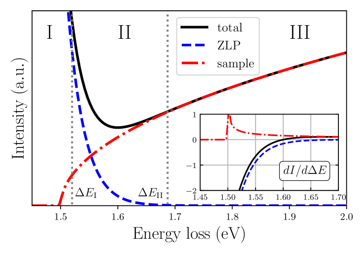
Figure 3.3: A toy model for the EEL spectrum and its derivative (in the inset). We display the separate contributions from $I_{\rm ZLP}$ and $I_{\rm inel}$ as well as their sum (total). We indicate the two regions used for the model training ($\rm I$ and $\rm III$), while as discussed in the text the neural network predictions are extrapolated to region $\rm II$, defined by $\Delta E_{\rm I}\leq\Delta E\leq\Delta E_{\rm II}$.

While simple, the toy model of Fig. 3.3 is actually general enough so that one can draw a number of useful considerations concerning the relation between $I_{\rm ZLP}$ and $I_{\rm inel}$ that will apply also in realistic spectra:

• The ZLP intensity, $I_{\rm ZLP}(\Delta E)$, is a monotonically decreasing function and thus its derivative is always negative.

• The first local minimum of the total intensity, $dI_{\rm EEL}/d\Delta E|_{\Delta E_{\rm min}}=0$, corresponds to a value of $\Delta E$ for which the contribution from the inelastic emissions is already sizable.

• The value of $\Delta E$ for which $I_{\rm inel}$ starts to contribute to the total spectrum corresponds to the position where the derivatives of the in-sample and in-vacuum intensities start to differ. We note that a direct comparison between the overal magnitude of the sample and vacuum ZLP spectra is in general not possible, as explained in Sect. 2.1.

These considerations suggest that when training the ML model on EEL spectra recorded on samples, the following categorisation should de adopted:

1. For energy losses $\Delta E\leq\Delta E_{\rm I}$ (region $\rm I$), the model training proceeds in exactly the same way as for the vacuum case via the minimisation of Eq. (3.11).

2. For $\Delta E\geq\Delta E_{\rm II}$ (region $\rm III$), we use instead Eq. (3.12) without the contribution from the input data, since for such values of $\Delta E$ one has that $I_{\rm inel}\gg I_{\rm ZLP}$. In other words, the only information that the region $\rm III$ provides on the model is the one arising from the implementation of the constraint that $I_{\rm ZLP}(\Delta E\to\infty)\to 0$.

3. The EELS measurements in region $\rm II$, defined by $\Delta E_{\rm I}\leq\Delta E\leq\Delta E_{\rm II}$, are excluded from the training dataset, given that in this region the contribution to $I_{\rm EEL}$ coming from $I_{\rm inel}$ is significant. There the model predictions are obtained from an interpolation of the associated predictions obtained in the regions $\rm I$ and $\rm III$.

The categorisation introduced in Fig. 3.3 relies on two hyper-parameters of the model, $\Delta E_{\rm I}$ and $\Delta E_{\rm II}$, which need to be specified before the training takes place. They should satisfy $\Delta E_{\rm I}\leq\Delta E_{\rm min}$ and $\Delta E_{\rm II}\geq\Delta E_{\rm min}$, with $\Delta E_{\rm min}$ being the position of the first local minimum of $I_{\rm EEL}$. As indicated by the toy spectra of Fig. 3.3, a suitable value for $\Delta E_{\rm I}$ would be somewhat above the onset of the inelastic contributions, to maximise the amount of training data while ensuring that $I_{\rm EEL}$ is still dominated by $I_{\rm ZLP}$.

The optimal value of $\Delta E_{\rm I}$ can be determined as follows. We evaluate the ratio between the derivative of the intensity distribution acquired on the specimen over the same quantity recorded in vacuum,

$$\mathcal{R}^{(j)}_{\rm der}(\Delta E)\equiv\left\langle{{dI_{\rm EEL}^{({\rm exp})(j)}(\Delta E)/d\Delta E}\over{dI_{\rm EEL}^{({\rm exp})(j^{\prime})}(\Delta E)/d\Delta E}}\right\rangle_{N_{\rm sp}^{\prime}}\,,$$ (3.17)

where $j^{\prime}$ labels one of the $N_{\rm sp}^{\prime}$ vacuum spectra and the average is taken over all available values of $j^{\prime}$. This ratio allows one to identify a suitable value of $\Delta E_{\rm I}$ by establishing for which energy losses the shape (rather than the absolute value) of the intensity distributions recorded on the specimen starts to differ significantly from their vacuum counterparts. A sensible choice of $\Delta E_{\rm I}$ could for instance be given by $\mathcal{R}_{\rm der}(\Delta E_{\rm I})\simeq 0.8$, for which derivatives differ at the 20% level. Note also that the leftmost value of the energy loss satisfying $\mathcal{R}_{\rm der}(\Delta E)=0$ in Eq. (3.17) corresponds to the position of the first local minimum.

Concerning the choice of the second hyper-parameter $\Delta E_{\rm II}$, following the discussion above one can identify $\Delta E_{\rm II}=\Delta E_{\rm pd}^{\rm(min)}$, which is determined by requiring that Eq. (3.13) satisfies $\mathcal{R}_{\rm sig}(\Delta E_{i})\mathrel{\hbox to0.0pt{\lower 4.0pt\hbox{\hskip 1.0pt$\sim$}\hss}\raise 1.0pt\hbox{$<$}}1$ and thus correspond to the value of $\Delta E$ where statistical uncertainties drown the signal intensity.

4 ZLP parametrisation from vacuum spectra

We now move to discuss the application of the strategy presented in the previous section to the parametrisation of ZLP spectra acquired in vacuum. Applying our model to this case has a two-fold motivation. First of all, we aim to demonstrate that the model is sufficiently flexible to effectively reproduce the input EELS measurements for a range of variations of the operation parameters of the microscope. Second, it allows one to provide a calibrated prediction useful for the case of the in-sample measurements. Such calibration is necessary since, as explained in Sect. 3.3, some of the model hyper-parameters are determined by comparing intensity shape profiles between spectra taken in vacuum and in sample.

In this section, first of all we present the input dataset and motivate the choice of training settings and model hyperparameters. Then we validate the model training by assessing the fit quality. Lastly, we study the dependence of the model output in its various input variables, extrapolate its predictions to new operation conditions, and study the dependence of the model uncertainties upon restricting the training dataset.

4.1 Training settings

In Table 4.1 we collect the main properties of the EELS spectra acquired in vacuum to train the neural network model. For each set of spectra, we indicate the exposure time $t_{\rm exp}$, the beam energy $E_{b}$, the number of spectra $N_{\rm sp}$ recorded for these operation conditions, the number $n_{\rm dat}$ of bins in each spectrum, the range in electron energy loss $\Delta E$, and the average full width at half maximum (FWHM) evaluated over the $N_{\rm sp}$ spectra with the corresponding standard deviation. The spectra listed on Table 4.1 were acquired with a ARM200F Mono-JEOL microscope equipped with a GIF continuum spectrometer, see also Methods. We point out that since here we are interested in the low-loss region, $\Delta E_{\rm max}$ does not need to be too large, and anyway the asymptotic $\Delta E$ behaviour of the model is fixed by the constraint implemented by Eq. (3.12).

Set	$t_{\rm exp}$ (ms)	$E_{\rm b}$ (keV)	$N_{\rm sp}$	$n_{\rm dat}$	$\Delta E_{\rm min}$ (eV)	$\Delta E_{\rm max}$ (eV)	FWHM (meV)
1	100	200	15	2048	-0.96	8.51	$47\pm 7$
2	100	60	7	2048	-0.54	5.59	$50\pm 4$
3	10	200	6	2048	-0.75	5.18	$26\pm 3$
4	10	60	6	2048	-0.40	4.78	$34\pm 2$

Table 4.1: Summary of the main properties of the EELS spectra acquired in vacuum to train the neural network model. For each set of spectra, we indicate the exposure time $t_{\rm exp}$, the beam energy $E_{b}$, the number of spectra $N_{\rm sp}$ recorded for these operation conditions, the number $n_{\rm dat}$ of bins in each spectrum, the range in electron energy loss $\Delta E$, and the average FWHM evaluated over the $N_{\rm sp}$ spectra with the corresponding standard deviation

The energy resolution of these spectra, quantified by the average value of their FWHM, ranges from 26 meV to 50 meV depending on the specific operation conditions of the microscope, with an standard deviation between 2 and 7 meV. The value of the FWHM varies only mildly with the value of the beam energy $E_{b}$ but grows rapidly for spectra collected with larger exposure times $t_{\rm exp}$. A total of almost $7\times 10^{4}$ independent measurements will be used for the ZLP model training on the vacuum spectra. As will be highlighted in Sects. 4.3 and 4.4, one of the advantages of our ZLP model is that it can extrapolate its predictions to other operation conditions beyond the specific ones used for the training and listed in Table 4.1.

Following the strategy presented in Sect. 3, first of all we combine the $N_{\rm sp}$ spectra corresponding to each of the four sets of operation conditions and determine the statistical uncertainty associated to each energy loss bin by means of Eq. (3.8). For each of the training sets, we need to determine the value of $\Delta E_{\rm pd}^{\rm(min)}~{}(=\Delta E_{\rm II})$ that defines the range for which we add the pseudo-data that imposes the correct $\Delta E\to\infty$ limit of the model. This value is fixed by the condition that ratio between the central experimental value of the EELS intensity and its corresponding uncertainty, Eq. (3.13), satisfies $\mathcal{R}_{\rm sig}\simeq 1$.

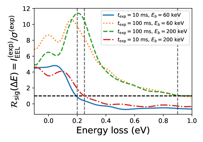
Figure 4.1: The ratio $\mathcal{R}_{\rm sig}(\Delta E)$ between the central experimental value of the EELS intensity distribution and its corresponding uncertainty, Eq. (3.13). Results are shown for the four combinations of $t_{\rm exp}$ and $E_{b}$ listed in Table 4.1. The vertical dashed lines mark the values of $\Delta E$ for which $\mathcal{R}_{\rm sig}\simeq 1$, which indicates when the data is dominated by statistical noise.

Fig. 4.1 displays this ratio for the four combinations of $t_{\rm exp}$ and $E_{b}$ listed in Table 4.1. The vertical dashed lines indicate the values of $\Delta E$ for which $\mathcal{R}_{\rm sig}$ becomes smaller than unity. For larger $\Delta E$, the EELS spectra become consistent with zero within uncertainties and can thus be discarded and replaced by the pseudo-data constraints. The total uncertainty of the pseudo-data points is then chosen to be

$$\sigma_{j}^{(\rm pd)}={{1}\over{10}}I_{{\rm EEL}}^{\rm(exp)}\left(\Delta E=\Delta E_{\rm pd}^{\rm(min)}\right)\,,\quad j=1,\ldots,N_{\rm pd}\,.$$ (4.1)

The factor of 1/10 is found to be suitable to ensure that the constraint is enforced without distorting the training to the experimental data. We observe from Fig. 4.1 that $\Delta E_{\rm pd}^{\rm(min)}$ depends the operation conditions, with $\Delta E_{\rm pd}^{\rm(min)}\simeq 200$ meV for $t_{\rm exp}=10$ ms and $\simeq 900$ meV for 100 ms, roughly independent on the value of the beam energy $E_{b}$.

The input experimental measurements listed in Table 4.1 are used to generate a sample of $N_{\rm rep}=500$ Monte Carlo replicas and to train an individual neural network to each of these replicas. The end result of the procedure is a set of model replicas,

$$I_{\rm ZLP}^{\rm(mod)(k)}(\Delta E,E_{b},t_{\rm exp})\,,\quad k=1,\ldots,N_{\rm rep}\,,$$ (4.2)

which can be used to provide a prediction for the intensity of the ZLP for arbitrary values of $\Delta E$, $E_{b}$, and $t_{\rm exp}$. Eq (4.2) provides the sought-for representation of the probability density in the space of ZLP models. By means of this sample of replicas, one can evaluate statistical estimators such as averages, variances, and correlations (as well as higher moments) as follows:

$$\left\langle I_{\rm ZLP}^{\rm(mod)}(\{z_{1}\})\right\rangle={{1}\over{N_{\rm rep}}}\sum_{k=1}^{N_{\rm rep}}I_{\rm ZLP}^{\rm(mod)(k)}(\{z_{1}\})\,,$$ (4.3)

$$\sigma_{I_{\rm ZLP}}^{\rm(mod)}(\{z_{1}\})=\left({{1}\over{N_{\rm rep}-1}}\sum_{k=1}^{N_{\rm rep}}\left(I_{\rm ZLP}^{\rm(mod)(k)}-\left\langle I_{\rm ZLP}^{\rm(mod)}\right\rangle\right)\right)^{1/2}\,,$$ (4.4)

$$\rho\left(\{z_{1}\},\{z_{2}\}\right)={{\left\langle I_{\rm ZLP}^{\rm(mod)}(\{z_{1}\})I_{\rm ZLP}^{\rm(mod)}(\{z_{2}\})\right\rangle-\left\langle I_{\rm ZLP}^{\rm(mod)}(\{z_{1}\})\right\rangle\left\langle I_{\rm ZLP}^{\rm(mod)}(\{z_{2}\})\right\rangle}\over{\sigma_{I_{\rm ZLP}}^{\rm(mod)}(\{z_{1}\})\sigma_{I_{\rm ZLP}}^{\rm(mod)}(\{z_{2}\})}}\,,$$ (4.5)

where as in the previous section $\{z_{l}\}$ denotes a possible set of input variables for the model, here $\{z_{l}\}=\left(\Delta E_{l},E_{b,l},t_{{\rm exp},l}\right)$.

4.2 Fit quality

We would like now to evaluate the overall fit quality of the neural network model and demonstrate that it is flexible enough to describe the available input datasets. In Table 4.2 we indicate the values of the final $\chi^{2}$ per data point, Eq. (3.14), as well as the average values of the cost function Eq. (3.11) evaluated over the training and validation subsets, for each of the four sets of spectra listed in Table 4.1 as well as for the total dataset. We recall that for a satisfactory training one expects $\chi^{2}\simeq 1$ and $\left\langle E_{\rm tr}\right\rangle\simeq\left\langle E_{\rm val}\right\rangle\simeq 2$ [59]. From the results of this table we find that, while our values are consistent with a reasonably good training, somewhat lower values than expected are obtained, for instance $\chi^{2}_{\rm tot}\simeq 0.8$ for the total dataset. This suggests that correlations between the input data points might be partially missing, since neglecting them often results into a moderate overestimate of the experimental uncertainties.

Set	$\qquad\chi^{2}\qquad$	$\qquad\left\langle E_{\rm tr}\right\rangle\qquad$	$\qquad\left\langle E_{\rm val}\right\rangle\qquad$
1	1.00	1.70	1.97
2	0.73	1.41	1.77
3	0.70	1.39	1.80
4	0.60	1.20	1.76
Total	0.77	1.47	1.85

Table 4.2: The values of the $\chi^{2}$ per data point, Eq. (3.14), as well as the average values of the cost function Eq. (3.11) over the training $\left\langle E_{\rm tr}\right\rangle$ and validation $\left\langle E_{\rm val}\right\rangle$ subsets, for each of the four sets of spectra listed in Table 4.1 as well as for the total dataset used in the present analysis.

Then Fig. 4.2 displays separately the $\chi^{2}$ distributions evaluated for the training and validation sets of the $N_{\rm rep}=500$ replicas of the sample trained on the spectra listed in Table 4.1. Note that the training/validation partition differs at random for each replica. The $\chi^{2}_{\rm tr}$ distribution peaks at $\chi^{2}_{\rm tr}\simeq 0.7$, indicating that a satisfactory model training has been achieved, but also that the errors on the input data points might have been slightly overestimated. We emphasize that the stopping criterion for the neural net training adopted here never considers the absolute values of the error function and determines proper learning entirely from the global minima of $E_{\rm val}^{(k)}$. From Fig. 4.2 we also observe that the validation distribution peaks at a slighter higher value, $\chi^{2}_{\rm val}\simeq 1$, and is broader that its corresponding training counterpart. These results confirm both that a satisfactory model training that prevents overlearning has been achieved as well as an appropriate estimate of the statistical uncertainties associated to the original EEL spectra.

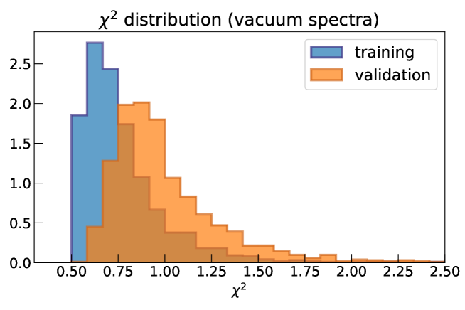
Figure 4.2: The distribution of the $\chi^{2}$ per data point evaluated separately for the training and validation sets over the $N_{\rm rep}=500$ replicas trained on the spectra listed in Table 4.1.

4.3 Dependence on the electron energy loss

Having demonstrated that our neural network model provides a satisfactory description of the input EEL spectra, we now present its predictions for specific choices of the input parameters. First of all, we investigate the dependence of the results as a function of the electron energy loss. Fig. 4.3 displays the central value and 68% confidence level uncertainty band for the ZLP model as a function of electron energy loss $\Delta E$ evaluated using Eqns. (4.3) and (4.4). We display results corresponding to three different values of $E_{b}$ and for both $t_{\rm exp}=10$ ms and $100$ ms. We emphasize that no measurements with $E_{b}=120$ keV have been used in the training and thus our prediction in that case arises purely from the model interpolation. It is interesting to note how both the overall normalisation and the shape of the predicted ZLP depend on the specific operating conditions.

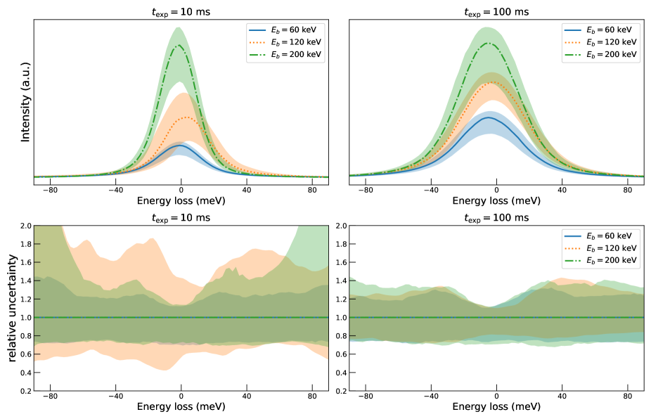
Figure 4.3: Top: the central value and 68% confidence level uncertainty band for the ZLP model as a function of electron energy loss $\Delta E$ evaluated using Eqns. (4.3) and (4.4). We display results corresponding to three different values of $E_{b}$ and for both $t_{\rm exp}=10$ ms (left) and $t_{\rm exp}=100$ ms (right panel). Note that no training data with $E_{b}=120$ keV has been used and thus our prediction in that case arises purely from the model interpolation. Bottom: the corresponding relative uncertainty as a function of $\Delta E$ for each of the three values of $E_{b}$.

In the bottom panels of Fig. 4.3 we show the corresponding relative uncertainties as a function of $\Delta E$ for each of the three values of $E_{b}$. Recall that in this work we allow for non-Gaussian distributions and thus the central value is the median of the distribution and the error band in general will be asymmetric. In the case of the $t_{\rm exp}=10$ ms results, we see how the model prediction at $E_{b}=120$ keV typically exhibits larger uncertainties than the predictions for the two values of $E_{b}$ for which we have training data. In the case of $t_{\rm exp}=100$ ms instead, the model predictions display very similar uncertainties for the three values of $E_{b}$, which furthermore depend only mildly on $\Delta E$. One finds there that the uncertainties associated to the ZLP model are $\simeq 20\%$ for $|\Delta E|\mathrel{\hbox to0.0pt{\lower 4.0pt\hbox{\hskip 1.0pt$\sim$}\hss}\raise 1.0pt\hbox{$<$}}100~{}{\rm meV}$.

For the purpose of the second part of this work, it is important to assess how the model results are modified once a subset of the data points are excluded from the fit. As illustrated in Fig. 3.3, when training the model on sample spectra, the region defined by with $\Delta E_{\rm I}\leq\Delta E\leq\Delta E_{\rm II}$ will be removed from the training dataset to avoid the contamination from the inelastic contributions. To emulate the effects of such cut, Fig. 4.4 displays the relative uncertainty in the model predictions for $I_{\rm ZLP}(\Delta E)$ as a function of the energy loss for $E_{b}=200$ keV and $t_{\rm exp}=10$ ms and 100 ms. We show results for three different cases: first of all, one without any cut in the training dataset, and then for two cases where data points with $\Delta E\geq\Delta E_{\rm cut}$ are removed from the training dataset. We consider two values of $\Delta E_{\rm cut}$, namely 50 meV and 100 meV, indicated with vertical dash-dotted lines. In both cases, data points are removed up until $\Delta E=$ 800 meV. The pseudo-data points that enforce the $I_{\rm EEL}(\Delta E)\to 0$ condition are present in all three cases in the region 800 meV $\leq\Delta E\leq 1~{}{\rm eV}$.

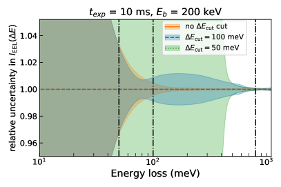
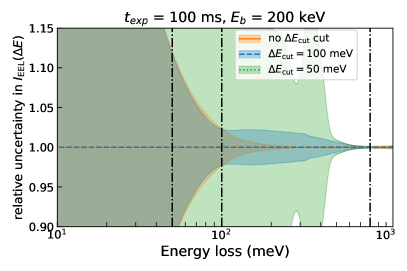
Figure 4.4: The relative uncertainty in the model predictions for $I_{\rm EEL}(\Delta E)$ as a function of the energy loss for $E_{b}=200$ keV and $t_{\rm exp}=10$ ms (left) and 100 ms (right panel). We show results for three different cases: without any cut in the training dataset, and where the data points with $\Delta E\geq\Delta E_{\rm cut}$ are removed from the training dataset for two different values of $\Delta E_{\rm cut}$. The same pseudo-data points that enforce $I_{\rm EEL}(\Delta E)\to 0$ are present in all three cases.

From this comparison one can observe how the model predictions become markedly more uncertain once a subset of the training data is cut away, as expected due to the effect of the information loss. While for the cut $\Delta E_{\rm cut}=100$ meV the increase in model uncertainty is only moderate as compared with the baseline fit where no cut is performed (since for this value of $\Delta E$ uncertainties are small to begin with), rather more dramatic effects are observed for a value of the cut $\Delta E_{\rm cut}=50$ meV. This comparison highlights how ideally we would like to keep as many data points in the training set for the ZLP model, provided of course one can verify that the possible contributions to the spectra related to inelastic scatterings from the sample can be neglected.

4.4 Dependence on beam energy and exposure time

As indicated in Table 4.1, the training dataset contains spectra taken at two values of the electron beam energy, $E_{b}=60$ keV and 200 keV. The left panel of Fig. 4.5 displays the predictions for the FWHM of the zero-loss peak (and its corresponding uncertainty) as a function of the beam energy $E_{b}$ for two values of the exposure time, $t_{\rm exp}=10$ ms and 100 ms. The vertical dashed lines indicate the two values of $E_{b}$ for which spectra are part of the training dataset. This comparison illustrates how the model uncertainty differs between the data region (near $E_{b}=60$ keV and 200 keV), the interpolation region (for $E_{b}$ between 60 and 200 keV), and the extrapolation regions (for $E_{b}$ below 60 keV and above 200 keV). In the case of $t_{\rm exp}=100$ ms for example, we observe that the model interpolates reasonably well between the measured values of $E_{b}$ and that uncertainties increase markedly in the extrapolation region above $E_{b}=200$ keV.

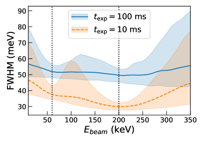
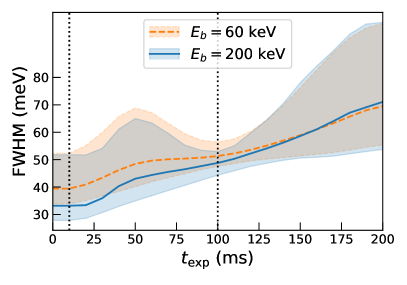
Figure 4.5: The model predictions for the FWHM of the zero-loss peak with its corresponding uncertainty as a function of the beam energy $E_{b}$ for two values of the exposure time (left panel) and as a function of $t_{\rm exp}$ for two values of $E_{b}$ (right panel). The vertical dashed lines indicate the values of the corresponding microscope operation parameter for which we have training data.

From this comparison one can also observe how as expected the uncertainty in the prediction for the FWHM of the ZLP is the smallest close to the values of $E_{b}$ for which one has training data. The uncertainties increase but only in a moderate way in the interpolation region, indicating that the model can be applied to reliably predict the features of the ZLP for other values of the electron energy beam (assuming that all other operation conditions of the microscope are unchanged). The errors then increase rapidly in the extrapolation region, which is a characteristic (and desirable) feature of neural network models. Indeed, as soon as the model departs from the data region there exists a very large number of different functional form models for $I_{\rm ZLP}(\Delta E)$ that can describe equally well the training dataset, and hence a blow up of the extrapolation uncertainties is generically expected.

In the same way as for the case of the electron beam energy $E_{b}$, while our ZLP model was trained on data with only exposure times of $t_{\rm exp}=10$ and $100$ ms, it can be used to reliably inter- and extrapolate to other values of $t_{\rm exp}$. The right panel of Fig. 4.5 displays the same comparison as in the left one now as a function of $t_{\rm exp}$ for $E_{b}=60$ keV and $E_{b}=200$ keV. We observe that the FWHM increases approximately in a linear manner with the exposure time, indicating that lower values of $t_{\rm exp}$ allow for an improved spectral resolution, and that the model predictions are approximately independent of $E_{b}$. Similarly to the predictions for varying beam energies, also for the exposure time the uncertainties grow bigger as the value of this parameter deviates more from the training inputs, specially for large values of $t_{\rm exp}$.

All in all, we conclude that the predictions of the ML model trained on vacuum spectra behave as they ought to: the smallest uncertainties correspond to the parameter values that are included in the training dataset, while the largest uncertainties arise in the extrapolation regions when probing regions of the parameter space far from those present in the training set.

5 Mapping low-loss EELS in polytypic WS₂

Following the discussion of the vacuum ZLP analysis, we now present the application of our machine learning strategy to parametrise the ZLP arising in spectra recorded on specimens, specifically for EELS measurements acquired in different regions of the WS₂ nanoflowers presented in Sect. 2.2. The resulting ZLP parametrisation will be applied to isolate the inelastic contribution in each spectrum. We will use these subtracted spectra first to determine the bandgap type and energy value from the behaviour of the onset region and second to identify excitonic transitions at very low energy losses.

In this section we begin by presenting the training dataset, composed by two groups of EEL spectra recorded in thick and thin regions of the WS₂ nanoflowers respectively. Then we discuss the subtraction procedure, the choice of hyper-parameters, and the error propagation to the physical predictions. The resulting subtracted spectra provide the information required to extract the value and type of the bandgap and to characterise excitonic transitions for different regions of these polytypic WS₂ nanostructures.

5.1 Training dataset

Low-magnification TEM images and the corresponding spectral images of two representative regions of the WS₂ nanoflowers, denoted as sample A and B respectively, are displayed in Fig. 5.1. These spectral images have been recorded in the regions marked by a green square in the associated TEM images, and contain an individual EEL spectrum in each pixel. We indicate the specific locations where EEL spectra have been recorded, including the in-vacuum measurements acquired for calibration purposes. Note that in sample B the differences in contrast are related to the material thickness, with higher contrast corresponding to thinner regions.

These two samples are characterised by rather different structural morphologies. While sample A is composed by a relatively thick region of WS₂, sample B corresponds to a region where thin petals overlap between them. In other words, sample A is composed by bulk WS₂ while in sample B some specific regions could be rather thinner, down to the few monolayers level. This thickness information has been be determined by means of the Digital Micrograph software.

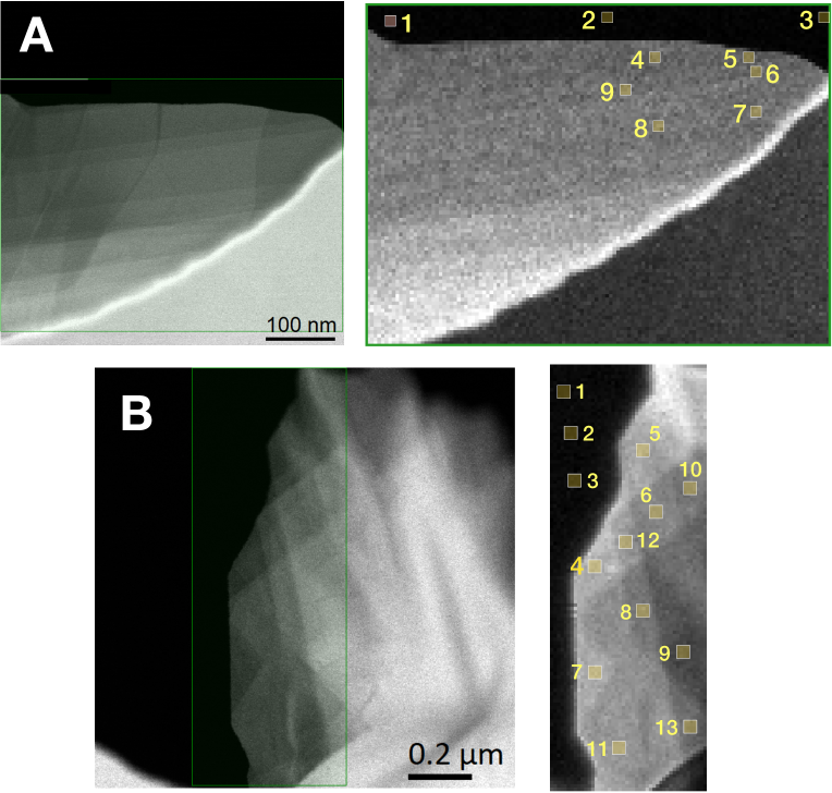
Figure 5.1: Low-magnification TEM images (left) and the corresponding spectral images (right panels) of two different regions of the WS₂ nanoflowers, denoted as sample A (upper) and sample B (lower panels) respectively. The spectral images have been recorded in the regions marked by a green square in the associated TEM images, and contain an individual EEL spectrum in each pixel. We indicate the locations where representative EEL spectra have been selected. In the left panel of sample B, the difference in contrast is correlated to the material thickness, with higher contrast indicating thinner regions of the nanostructure. The morphological differences between the two samples are discussed in the text.

One of the main goals of this study is demonstrating that our ZLP-subtraction method exhibits a satisfactory performance for spectra taken with different microscopes and operation conditions. With this motivation, the EELS measurements acquired on specimens A and B have been obtained varying both the microscopes and their settings. Specifically, the TEM and EELS measurements acquired in specimen A are based on a JEOL 2100F microscope with a cold field-emission gun and equipped with an aberration corrector, operated at 60 kV and where a Gatan GIF Quantum was used for the EELS analysis. The corresponding measurements on specimen B were recorded instead using a JEM ARM200F monochromated microscope operated at 60 kV and equipped with a GIF quantum ERS. See Methods for more details.

In Table 5.1 we collect the most relevant properties of the spectra collected in the locations indicated in Fig. 5.1 using the same format as in Table 4.1. As we just mentioned, the spectra from samples A and B have been acquired with different microscopes and thus features of the ZLP such as the FWHM are expected to be different. From this table one can observe how the ZLP for the spectra acquired on sample A exhibit a FWHM about five times larger as compared to those of sample B. This difference in energy resolution can be understood from the fact that the EELS spectra from sample B, unlike those from sample A, were recorded with a TEM equipped with monochromator.

Set	$t_{\rm exp}$ (ms)	$E_{\rm b}$ (keV)	$N_{\rm sp}$	$N_{\rm dat}$	$\Delta E_{\rm min}$ (eV)	$\Delta E_{\rm max}$ (eV)	FWHM (meV)
A	1	60	6	1918	-4.1	45.5	$470\pm 10$
B	190	60	10	2000	-0.9	9.1	$87\pm 5$

Table 5.1: Same as Table 4.1 for the EEL spectra taken on specimens A and B. The location on the WS₂ nanoflowers where each spectra has been recorded is indicated in Fig. 5.1.

In the following we will present results for representative spectra corresponding to specific choices of the locations indicated in Fig. 5.1. The full set of recorded spectra is available within EELSfitter, the code used to produce the results of this analysis, and whose installation and usage instructions are summarised in Appendix A.

5.2 Subtraction procedure

In Table 5.2 we collect the mean value and uncertainty of the first local minimum, $\Delta E|_{\rm min}$. averaged over the spectra corresponding to samples A and B from Fig. 5.1. The location of the first minimum is relatively stable among all the spectra belonging to a given set. This indicates that the onset of the inelastic contributions $I_{\rm inel}$ does not change significantly as we move between different regions of the sample. We also indicate there the corresponding values of the hyper-parameters $\Delta E_{\rm I}$ and $\Delta E_{\rm II}$ defined in Fig. 3.3. Recall that only the data points with $\Delta E\leq\Delta E_{\rm I}$ are used for the training of the neural network model. The model training is performed for a range of $\Delta E_{\rm I}$ values, subject to the condition that $\Delta E_{\rm I}\leq\Delta E_{\rm min}$, to validate the stability of the results. The optimal value of $\Delta E_{\rm I}$ is determined by the condition that Eq. (3.17) satisfies $\mathcal{R}^{(j)}_{\rm der}(\Delta E)\simeq 0.9$, indicating that the shape of the intensity profile for the sample spectra differs by more than 10% as compared to their vacuum counterparts.

Set	$\Delta E|_{\rm min}$ (eV)	$\Delta E_{\rm I}$ (eV)	$\Delta E_{\rm II}$ (eV)
A	$2.70\pm 0.06$	1.8	12
B	$1.80\pm 0.04$	1.4	6

Table 5.2: The mean value and uncertainty of the first local minima, $\Delta E|_{\rm min}$, averaged over the spectra corresponding to samples A and B from Fig. 5.1. We also indicate the corresponding values of the hyper-parameters $\Delta E_{\rm I}$ and $\Delta E_{\rm II}$ defined in Fig. 3.3 used for the training of the neural network model.

In the region $\Delta E\geq\Delta E_{\rm II}$, the training set includes only the pseudo-data that implements the $I_{\rm ZLP}(\Delta E)\to 0$ constraint. The values for $\Delta E_{\rm II}$ were determined from the spectra recorded in vacuum following the same procedure as explained in Sect. 4, based on requiring $\mathcal{R}_{\rm sig}(\Delta E_{\rm II})\mathrel{\hbox to0.0pt{\lower 4.0pt\hbox{\hskip 1.0pt$\sim$}\hss}\raise 1.0pt\hbox{$<$}}1$. We note that the values of $\Delta E_{\rm II}$ found now are significantly higher than the ones obtained in Fig. 4.1 for the vacuum case. This difference could be ascribed to the fact that the vacuum spectra from samples A and B were recorded in proximity to the sample so that the influence of the specimen is still partially felt.

The end result of the neural network training described in Sect. 3.3 is a set of $N_{\rm rep}=500$ replicas parametrising the zero-loss peak,

$$I_{\rm ZLP}^{({\rm mod})(k)}(\Delta E)\,,\quad k=1,\ldots,N_{\rm rep}\,.$$ (5.1)

Taking into account that we have $N_{\rm sp}$ individual spectra in each sample, the ZLP subtraction is performed individually for each Monte Carlo replica,

$$I_{\rm inel}^{({\rm exp})(j,k)}(\Delta E)\equiv I_{\rm EEL}^{({\rm exp})(j)}(\Delta E)-I_{\rm ZLP}^{({\rm mod})(k)}(\Delta E)\,,\quad\forall~{}N_{\rm rep}\,,\quad j=1,\ldots,N_{\rm sp}\,,$$ (5.2)

from which statistical estimators can be evaluated. For instance, the mean value for our model prediction for the $j$-th spectrum can be evaluated by averaging over the replicas,

$$\left\langle I_{\rm inel}^{({\rm exp})(j)}\right\rangle(\Delta E)={{1}\over{N_{\rm rep}}}\sum_{k=1}^{N_{\rm rep}}I_{\rm inel}^{({\rm exp})(j,k)}(\Delta E)\,,\quad j=1,\ldots,N_{\rm sp}\,,$$ (5.3)

and likewise for the corresponding uncertainties and correlation coefficients. For large values of $\Delta E$, the model prediction reduces to the original spectra, since in that region the ZLP contribution vanishes,

$$I_{\rm inel}^{({\rm exp})(j,k)}(\Delta E\gg\Delta E_{\rm I})\to I_{\rm EEL}^{{\rm(exp)}(j)}(\Delta E)\,,\quad\forall~{}j,k\,.$$ (5.4)

For very small values of the energy loss, the contribution to the total spectra from inelastic scatterings is negligible and thus the subtracted model prediction Eq. (5.2) should vanish. However, this will not be the case in general since the neural network model is trained on the $N_{\rm sp}$ ensemble of spectra, rather that just on individual ones, and thus the expected $\Delta E\to 0$ behaviour will only be achieved within uncertainties rather than at the level of central values. To achieve the desired $\Delta E\to 0$ limit, we apply a matching procedure as follows. We introduce another hyper-parameter, $\Delta E_{0}<\Delta E_{\rm I}$, such that one has for the $k$-th ZLP replica associated to the $j$-th spectrum the following behaviour:

$$I_{\rm ZLP}^{({\rm mod})(j,k)}(\Delta E) = I_{\rm EEL}^{({\rm exp})(j)}(\Delta E)\,,\quad\Delta E<\Delta E_{0}\,,$$

$$I_{\rm ZLP}^{({\rm mod})(j,k)}(\Delta E) = I_{\rm EEL}^{{\rm(exp)}(j)}+\left(\xi_{1}^{(n_{l})(k)}(\Delta E)-I_{\rm EEL}^{{\rm(exp)}(j)}(\Delta E)\right)\times\mathcal{F}\,,\quad\Delta E_{0}<\Delta E\leq\Delta E_{\rm I}\,,$$ (5.5)

$$\mathcal{F}(\Delta E)=\exp\left(-{{\left(\Delta E-\Delta E_{\rm I}\right)^{2}}\over{\left(\Delta E_{0}-\Delta E_{\rm I}\right)^{2}\delta^{2}}}\right)\,,$$

$$I_{\rm ZLP}^{({\rm mod})(j,k)}(\Delta E) = \xi_{1}^{(n_{l})(k)}(\Delta E)\,,\quad\Delta E>\Delta E_{\rm I}\,,$$

where $\xi_{1}^{(n_{l})(k)}$ indicates the output of the $k$-th neural network that parametrises the ZLP and $\delta$ is a dimensionless tunable parameter. In Eq. (5.5), $\mathcal{F}(\Delta E)$ represents a matching factor that ensures that the ZLP model prediction smoothly interpolates between $\Delta E=\Delta E_{0}$ (where $\mathcal{F}\ll 1$ and the original spectrum should be reproduced) and $\Delta E=\Delta E_{\rm I}$ (where $\mathcal{F}=1$ leaving the neural network output unaffected). Here we adopt $\Delta E_{0}=\Delta E_{\rm I}-0.5\,{\rm eV}$, having verified that results are fairly independent of this choice. Taking into account the matching procedure, we can slightly modify Eq. (5.2) to

$$I_{\rm inel}^{({\rm mod})(j,k)}(\Delta E)\equiv I_{\rm EELS}^{({\rm exp})(j)}(\Delta E)-I_{\rm ZLP}^{({\rm mod})(j,k)}(\Delta E)\,,\quad\forall~{}N_{\rm rep}\,,\quad j=1,\ldots,N_{\rm sp}\,.$$ (5.6)

The ensemble of ZLP-subtracted spectra obtained this way, $\{I_{\rm inel}^{({\rm mod})(j,k)}\}$, can then be used to reliably extract physical information from the low-loss region of the spectrum.

5.3 Bandgap analysis of polytypic 2H/3R WS₂

One particularly important application of the ZLP-subtracted spectra is to estimate the specimen bandgap in the region where they were acquired. Different approaches have been put forward to evaluate $E_{\rm BG}$ from subtracted EEL spectra, e.g. by means of the inflection point of the rising intensity or a linear fit to the maximum positive slope [61]. Here we will adopt the approach of [12] where the behaviour of $I_{\rm inel}(\Delta E)$ in the onset region is modeled as

$$I_{\rm inel}(\Delta E)\simeq A\left(\Delta E-E_{\rm BG}\right)^{b}\,,\quad\Delta E\geq E_{\rm BG}\,,$$ (5.7)

and vanishes for $\Delta E<E_{\rm BG}$, where both the bandgap value $E_{\rm BG}$ as well as the parameters $A$ and $b$ are extracted from the fit. The exponent $b$ is expected to be $b\simeq 1/2~{}(\simeq 3/2)$ for a semiconductor material characterised by a direct (indirect) bandgap. For each of the $N_{\rm sp}$ spectra and the $N_{\rm rep}$ replicas we fit to Eq. (5.6) the model Eq. (5.7) within a range taken to be $\left[\Delta E_{\rm I}-0.5~{}{\rm eV},\Delta E_{\rm I}+0.7~{}{\rm eV}\right]$. One ends up with $N_{\rm rep}$ values for the bandgap energy and fit exponent for each spectra,

$$\Big{\{}E_{\rm BG}^{(j,k)},b^{(j,k)}\Big{\}}\,,\quad k=1,\ldots,N_{\rm rep}\,,\quad j=1,\ldots,N_{\rm sp}\,,$$ (5.8)

from which again one can readily evaluate their statistical estimators. In the following, we will display the median and the 68% confidence level intervals for these parameters to account for the fact that their distribution will be in general non-Gaussian.

Here we present the results for the bandgap analysis of sample A, taking location sp4 in Fig. 5.1 as representative spectrum; compatible results are obtained for the rest of locations in this sample. As mentioned above, this region is characterised by a sizable thickness where WS₂ is expected to behave as a bulk material. The left panel of Fig. 5.2 displays the original and subtracted EEL spectrum together with the predictions of the ZLP model, where the bands indicate the 68% confidence level uncertainties and the central value is the median of the distribution. The inset shows the result of the polynomial fits using Eq. (5.7) to the subtracted spectrum together with the corresponding uncertainty bands.

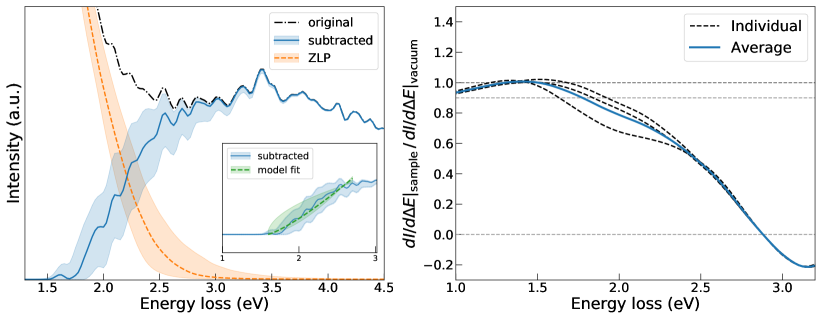
Figure 5.2: Left: the original and subtracted EEL spectra corresponding to location sp4 of sample A in Fig. 5.1, together with the predictions of the ZLP model, where the bands indicate the 68% confidence level uncertainties. The inset displays the result of fitting Eq. (5.7) to the onset region of the subtracted spectrum. Right: the average ratio of the derivative of the intensity distribution in sp4 over its vacuum counterparts, Eq. (3.17)

One can observe how the ZLP model uncertainties are small at low $\Delta E$ (due to the matching condition) and large $\Delta E$ (where the ZLP vanishes), but become significant in the intermediate region where the contributions from $I_{\rm ZLP}$ and $I_{\rm inel}$ become comparable. It is worth emphasizing that these (unavoidable) uncertainties are neglected in most ZLP subtraction methods. The validity of our choice for the hyperparameter $\Delta E_{\rm I}$ (Table 5.2) can be verified a posteriori by evaluating the ratio

$$\mathcal{R}^{(j)}_{\rm abs}\left(\Delta E_{\rm I}\right)\equiv\left\langle I_{\rm ZLP}^{({\rm mod})(j)}\right\rangle_{\rm rep}\Big{/}I_{\rm EEL}^{({\rm exp})(j)}\Big{|}_{\Delta E=\Delta E_{\rm I}}\,,$$ (5.9)

which in this case turns out to be $\mathcal{R}_{\rm abs}=0.98$. It is indeed important to verify that $\mathcal{R}_{\rm abs}\left(\Delta E_{\rm I}\right)$ is not too far from unity, indicating that the training dataset has not been contaminated by the contributions arising from inelastic scatterings off the specimen.

The average ratio of the derivative of the intensity distribution in sp4 over its vacuum counterpart, Eq. (3.17), is shown in the right panel of Fig. 5.2. By requiring that $\mathcal{R}_{\rm der}(\Delta E_{\rm I})\simeq 0.9$ we obtain the value $\Delta E_{\rm I}=1.8$ eV used as baseline in the analysis. It should be noted that this choice is not unique, for example requiring $\mathcal{R}_{\rm der}(\Delta E_{\rm I})\simeq 0.8$ instead would have led to $\Delta E_{\rm I}=2.0$ eV. It is therefore important to asses the stability of our results as the hyper-parameter $\Delta E_{\rm I}$ is varied around its optimal value. With this motivation, in Fig. 5.3 we display the values of the exponent $b$ and the bandgap energy $E_{\rm BG}$ obtained from the same subtracted spectrum as that shown in Fig. 5.2 for variations of $\Delta E_{\rm I}$ around its optimal value (vertical dot-dashed line) by an amount of $\pm 0.2$ eV. We observe that the model predictions for both $b$ and $E_{\rm BG}$ are stable with respect to variations of $\Delta E_{\rm I}$, with shifts in central values contained within the uncertainty bands. We can thus conclude that our approach is robust with respect to the choice of hyper-parameters.

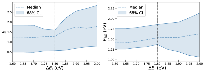
Figure 5.3: The values of the exponent $b$ (left) and the bandgap energy $E_{\rm BG}$ (right panel) from the model Eq. (5.7) obtained from the subtracted spectrum sp14 as $\Delta E_{\rm I}$ is varied by $\pm 0.2$ eV around its optimal value, indicated by the horizontal dot-dashed line.

The final values for $E_{\rm BG}$ and $b$ obtained in the analysis of this specific spectrum are

$$E_{\rm BG}=1.6_{-0.2}^{+0.3}\,{\rm eV}\,,\quad b=1.3_{-0.7}^{+0.3}\,.$$ (5.10)

We thus find that for this specific region of the WS₂ nanoflowers the model fit to the subtracted EEL spectrum exhibits a clear preference for an indirect bandgap (where $b\simeq 1.5$ is expected). This result is consistent with previous studies of the local electronic properties of bulk WS₂, such as those reported in Table 2.1. Consistent results are obtained for spectra acquired at other locations of Fig. 5.1; for example for sp5 one has

$$E_{\rm BG}=1.7\pm 0.2\,{\rm eV}\,,\quad b=1.3_{-0.4}^{+0.3}\,.$$ (5.11)

These results represent the first EELS-based bandgap determination of WS₂ nanostructures whose crystalline structure is based on mixed 2H/3R polytypes.

5.4 Mapping excitonic transitions in the low-loss region

For the application of our ZLP subtraction strategy to the EEL spectra recorded in specimen B of the WS₂ nanoflowers (bottom panels in Fig. 5.1), the same criterion based on the derivative ratio Eq. (3.17) to select the hyper-parameter $\Delta E_{\rm I}$ was used. In this case, one finds a value of $\Delta E_{\rm I}\simeq 1.4$ eV, somewhat lower than the corresponding value obtained for sample A. The left panel of Fig. 5.4 displays the original and subtracted spectra corresponding to the representative location sp4 of sample B together with the predictions of the ZLP model. As before, the bands indicate the 68% confidence level uncertainties and the central value is the median.

The main difference with respect to the spectra recorded in sample A is the appearance of well-defined features (peaks) in the subtracted spectrum already for very small values of $\Delta E$. In particular, we observe two marked peaks at $\Delta E\simeq 1.5$ and 2.0 eV and a softer one near $\Delta E\simeq 1.7$ eV. Further additional features arise also for higher values of the energy loss. There are two main sources for the observed differences between the spectra recorded in each sample. The first one is that, while sample A is much thicker (bulk material), sample B corresponds to thin, overlapping petals whose thicknesses can be as small as a few monolayers. The second is that the EELS measurements taken in sample A used a TEM without monochromator, while those in sample B benefited from a monochromator thus achieving a superior spectral resolution (with an average FWHM of 87 meV to be compared with the 470 meV of sample A, see Table 5.1). This combination of structural and morphological variations in the specimen together with the operation conditions of the TEM therefore should account for the most of differences between the two sets of spectra.

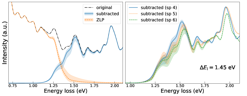
Figure 5.4: Left: the original and subtracted EEL spectra corresponding to location sp4 of sample B in Fig. 5.1, together with the predictions of the ZLP model. The bands indicate the 68% confidence level uncertainties. Right: comparison of the ZLP-subtracted spectra from locations sp4, sp5, and sp6 in sample B together with the corresponding model uncertainties. Note how several features of the subtracted spectra, in particular the peaks at $\Delta E\simeq 1.5$, 1.7 and 2.0 are eV, are common across the three locations.

It is worth noting here that our ZLP parametrisation and subtraction strategy exhibits a satisfactory performance for all the spectra under consideration, irrespective of the spectral resolution of the TEM used for their acquisition. By comparing Figs. 5.4 and 5.2, one observes that model uncertainties are larger in the latter case than in the former, as expected from the superior spectral resolution of the EELS measurements taken on sample B. Nevertheless, the same approach has been used in both cases without the need of any fine-tuning or ad hoc adjustments: of course, if the input spectra have been recorded with better spectral resolution, the resulting ZLP model uncertainties will improve accordingly without changing the procedure itself.

Given that the well-defined spectral features present in Fig. 5.4 appear close to the onset of the inelastic emissions, $I_{\rm inel}(\Delta E)$, these spectra are not suitable for bandgap determination analyses. The reason is that the method of [12] used in sample A is only applicable under the assumption that there is a sufficiently wide region in $\Delta E$ after the onset of $I_{\rm inel}$ to perform the polynomial fit of Eq. (5.7). This is clearly not possible for the spectra recorded in sample B, and indeed model fits restricted to $\Delta E\leq 1.4$ eV display a marked numerical instability. Instead of studying the bandgap properties, it is interesting to exploit the ZLP-subtracted results of sample B to characterise the local excitonic transitions of polytypic 2H/3R WS₂ that are known to arise in the ultra-low-loss region of the spectra.

Before being able to do this, however, one has to deal with the possible objection that the peaks present in Fig. 5.4 are not genuine features, but rather fluctuations due to insufficient statistics that should be smoothed out before this region can be interpreted. To tackle this concern, the right panel of Fig. 5.4 displays a comparison of the ZLP-subtracted spectra recorded in the (spatially separated) locations sp4, sp5 and sp6 in sample B together with their model uncertainties. Both the position and the widths of the peaks at $\Delta E\simeq 1.5$, 1.7 and 2.0 eV remain stable, confirming that these are genuine physical features rather than fluctuations.

These peaks in the ultra-low-loss region of the ZLP-subtracted EELS spectra recorded on thin, polytypic WS₂ nanostructures can be traced back to excitonic transitions. Their origin can be attributed to the formation of an electron-hole pair mitigated by the dielectric screening from the surrounding lattice [62]. In nanostructures with reduced dimensionality as well as in single layers of TMD materials, exciton peaks arise with binding energies up to ten times larger than for bulk structures. In the optical spectra of TMDs, two strongly pronounced resonances denoted by A and B excitons are often observed, appearing at binding energies of 300 and 500 meV below the true bandgap of the material [63]. Interestingly, this prediction is in agreement with the observed peaks at $\Delta E\simeq 1.5$ and 1.7 eV if one takes into account the expected value of $E_{\rm BG}$ for very thin WS₂ nanostructures, see Table 2.1

We conclude that ZLP-subtracted spectra in sample B allow one for a clean mapping of the exciton peaks present in the WS₂ nanoflowers down to $\Delta E\simeq 1.5$ eV together with the associated uncertainty estimate. Further insights concerning the relationship between the exciton peaks in the ultra-low-loss region and the underlying crystalline structure and specimen morphology could be obtained by combining our findings with ab initio calculations such as those based on density functional theory.

6 Summary and outlook

In this work we have presented a novel, model-independent strategy to parametrise and subtract the ubiquitous zero-loss peak that dominates the low-loss region of EEL spectra. Our strategy is based on machine learning techniques and provides a faithful estimate of the uncertainties associated to both the input data and the procedure itself, which can then be propagated to physical predictions without any approximations. We have demonstrated how, in the case of vacuum spectra, our approach is sufficiently flexible to accomodate several input variables corresponding to different operation conditions of the microscope. Further, we are able to reliably extrapolate our predictions, e.g. for the expected FWHM of the ZLP, to other operation conditions. When applied to spectra recorded on specimens, our approach makes possible to robustly disentangle the ZLP contribution from those arising from inelastic scatterings. Thanks to this subtraction, one can fully exploit the valuable physical information contained in the ultra low-loss region of the spectra.

Here we have applied this ZLP subtraction strategy to EEL spectra recorded in WS₂ nanoflowers characterised by a 2H/3R polytypic crystalline structure. First of all, measurements taken in a relatively thick region of the specimen were used to determine the local value of the bandgap energy $E_{\rm BG}$ and to assess whether this bandgap is direct or indirect. A model fit to the onset of the inelastic intensity distribution obtains $E_{\rm BG}\simeq 1.6^{+0.3}_{-0.2}\,{\rm eV}$ and exhibits a marked preference for an indirect bandgap. Our findings are consistent with previous studies, both of theoretical and of experimental nature, concerning the bandgap structure of bulk WS₂.

Subsequently, we have applied our method to a thinner region of the WS₂ nanoflowers, specifically a region composed by overlapping petals with varying thicknesses that can be as small as a few monolayers. We have demonstrated how for such specimens one can exploit the ZLP-subtracted results to characterise the local excitonic transitions that arise in the ultra-low-loss region. By charting the exciton peaks of 2H/3R polytypic WS₂ there, we identify two strong peaks at $\Delta E\simeq 1.5$ and 2 eV (and a softer one at 1.7 eV) and show how these features are consistent when comparing spatially-separated locations in sample B. Further, since our method provides an associated uncertainty estimate, one can robustly establish the statistical significance of each of these ultra-low-loss region features.

The approach presented in this work could be extended in several directions. First of all, it would be interesting to test its robustness when additional operation conditions of the microscope are included as input variables, and to verify to which extent the ZLP parametrisations obtained for an specific microscope can be generalised to an altogether different TEM. Further, a non-trivial cross-check of our method would be provided by validating our predictions for other operation conditions of the microscope, such as the FWHM as a function of the beam energy $E_{b}$ of the exposure time $t_{\rm exp}$ reported in Fig. 4.5, with actual measurements.

Concerning the physical interpretation of the low-loss region of EEL spectra, our method could be applied to study the bandgap properties for different types of nanostructures built upon TMD materials, such as MoS₂ nanowalls [64] and vertically-oriented nano-sheets [65] or WS₂/MoS₂ arrays, heterostructures, and ternary alloys. In addition to bandgap characterisation, this ZLP-subtraction strategy should allow the detailed study of other phenomena relevant for the interpretation of the low-loss region such as plasmons, excitons, phonon interactions, and intra-band transitions. One could also exploit the subtracted EEL spectra to further characterise local electronic properties by means of the evaluation of the complex dielectric function and its associated uncertainties in terms of the Kramers-Kronig relations. Finally, these phenomenological studies of local electronic properties should be compared with ab initio calculations based on the same underlying crystalline structure as the studied specimens.

Another possible application of the strategy presented in this work would be the automation of the study of spectral TEM images, such as those displayed in the right panels of Fig. 5.1, where each pixel contains an individual EEL spectrum. Here machine learning methods would provide a useful handle in order to identify relevant features of the spectra (peaks, edges, shoulders) with minimal human intervention (no need to process each spectrum individually) and then determine how these features vary as we move along different regions of the nanostructure. Such an approach would combine two important families of machine learning algorithms, those used for regression, in order to quantify the properties of spectral features such as width and significance, and those for classification, to identify categories of distinct features across the spectral image.

Acknowledgments

We are grateful to Emanuele R. Nocera and Jacob J. Ethier for assistance in installing EELSfitter in the Nikhef computing cluster. L. R. is grateful to Cas, Agneet, and Aar, for support under all (rainy) circumstances.

Funding

S. E. v. H. and S. C.-B. acknowledge financial support from the ERC through the Starting Grant “TESLA””, grant agreement no. 805021. L. M. acknowledges support from the Netherlands Organizational for Scientific Research (NWO) through the Nanofront program. The work of J. R. has been partially supported by NWO.

Declaration of competing interest

The authors declare that they have no known competing financial interests or personal relationships that could have appeared to influence the work reported in this paper.

Methods

The EEL spectra used for the training of the vacuum ZLP model presented in Sect. 4 were collected in a ARM200F Mono-JEOL microscope equipped with a GIF continuum spectrometer and operated at 60 kV and 200 kV. For these measurements, a slit in the monochromator of 2.8 $\mu$m was used. The TEM and EELS measurements acquired in Specimen A for the results presented in Sect. 5 were recorded in a JEOL 2100F microscope with a cold field-emission gun equipped with aberration corrector operated at 60 kV. A Gatan GIF Quantum was used for the EELS analyses. The convergence and collection semi-angles were 30.0 mrad and 66.7 mrad respectively. The TEM and EELS measurements acquired for Specimen B in Sect. 5 were recorded using a JEM ARM200F monochromated microscope operated at 60 kV and equipped with a GIF quantum ERS. The convergence and collection semi-angles were 24.6 mrad and 58.4 mrad respectively in this case, and the aperture of the spectrometer was set to 5 mm.

Supplementary Material

Appendix A Installation and usage of EELSfitter

In this appendix we provide some instructions about the installation and the usage of the EELSfitter code developed in this work. The code is available from its GitHub repository

https://github.com/LHCfitNikhef/EELSfitter

and is composed by a number of Python scripts. The code requires a working installation of Python3 and the following libraries: NumPy, TensorFlow (v2), pandas, SciPy and scikit-learn.

Load_data.py

This script reads the spectrum intensities and create data-frames to be used for training the neural network. It reads out the EEL spectra intensities, automatically selects the energy loss at which the peak intensity occurs and shifts the dataset such that the peak intensity is centered at $\Delta E=$0. Further, for each spectrum it returns the normalized intensity by normalizing over the total area under the spectrum. The output is two datasets, df and df_vacuum which contain the information on the in-sample and in-vacuum recorded spectra respectively. The user needs to upload the spectral data in .txt format to the ’Data’ folder and make sure that the vacuum and in-sample spectra are added to the appropriate one. For each of the spectra the minimum and maximum value of the recorded energy loss need to be set manually in Eloss_min and Eloss_max.

Fitter.ipynb

This script is used to run the neural network training on the data that was uploaded using load_data.py. It involves a number of pre-processing steps to determine the hyper-parameters $\Delta E_{\rm I}$ and $\Delta E_{\rm II}$ and then it automatically prepares and cuts the data before it is fed to the neural network to start the training. It is structured as follows:

• Importing libraries and spectral data from the load_data.py script.

• Evaluate $\Delta E_{\rm I}$ from the intensity derivatives. In order to determine the value for the hyper-parameter $\Delta E_{\rm I}$, a dataframe df_dx is created and it calculates the derivatives of each of the in-sample recorded spectra, stored as df_dx[’derivative y*’], where * is any of the in-sample recorded spectra. The first crossing of any of the derivatives with zero is determined and stored as the value of $\Delta E_{\rm I}$.

• Evaluate $\Delta E_{\rm II}$ for the pseudo-data. It calculates the mean over all vacuum spectra, df_mean, and the ratio of the intensity to the experimental uncertainty for each value of $\Delta E$, df_mean[’ratio’]. The value of $\Delta E_{\rm II}$ is then determined as the energy loss at which this ratio drops below 1 and is stored together with the value of $\Delta E_{\rm I}$ as the hyper-parameters for training. However, if one wishes to use other values for these parameters, for instance for cross-validating the best value for $\Delta E_{\rm I}$, these can also be adjusted manually.

• Experimental data processing. The next step is to keep only the data points with $\Delta E\leq\Delta E_{\rm I}$ and dropping the points with higher energy losses. Experimental central values and uncertainties are calculated by means of equal width discretization, for which the number of bins has to be set as nbins. The default value is 32, which means that 32 training inputs are spread equally over the range [$\Delta E_{\rm min},\Delta E_{\rm I}$]. Note that the logarithm of the intensity is used as training inputs, because this facilitates the optimization of the neural network ($I_{\rm EEL}$ being a steeply falling function of $\Delta E$). The code translates this back to the original intensity values after the training. $N_{\rm pd}$ pseudo datapoints are added in the range $[\Delta E_{\rm II},\Delta E_{\rm max}]$, where $\Delta E_{\rm max}$ is the maximum energy loss value of the recorded spectra. The values for $N_{\rm pd}$ and $\Delta E_{\rm max}$ should be changed manually by setting them in max_x and N_pseudo. The output is a dataframe df_full containing all training data and pseudo data points, corresponding to a total of $N_{\rm in}$ (= $n_{\rm bins}$ + $N_{\rm pd}$) training inputs.

• Initialize the NN model, where the code defines the neural network architecture and prepares the data inputs to feed them to the neural network for training. The function make_model() allows to define the number of hidden layers and nodes per layer. The default architecture is 1-10-15-5-1.

• Initialize data for NN training. Here the code prepares the recorded spectra to be used as inputs for the neural network. First, we initiate placeholders for the variables x, y and sigma which allow us to create our operations and build our computation graph, without needing the data itself. The dimension of the placeholder is defined by $[{\bf None},dim]$ where ’dim’ should be set to the dimension of the corresponding variable. In this case the input is one-dimensional, so dim=1. These placeholders are used to define predictions, which is in fact a placeholder that is used later to make predictions on inputs x. Also, we define a vector predict_x that is used to make a direct prediction after training on each of the replicas. It consists of $N_{\rm pred}$ data points in the energy loss range [pred_min, pred_max].

• Create the Monte Carlo replicas. The final step to be taken before we can start training is the creation of sample of $N_{\rm rep}$ Monte Carlo replicas of the original EEL spectra, following the procedure described in Sect. 3.2. This is done automatically using the experimental intensities train_y and uncertainties train_sigma for a total of Nrep replicas. The output is an ($N_{\rm in},N_{\rm rep}$) vector containing all the MC replicas.

• Train the neural networks. The final part of the script, where the NN training is carried out, is based on the function function_train() that implements the strategy presented in Sect. 3.3. The cost function, optimizer and learning rate are defined here, together with a ’saver’ used to save the network parameters after each optimization. We start a loop over Nrep replicas to initiate a training session on each of the individual replicas in series. For each iteration, the $k$-th replica is selected from the sample of $N_{\rm rep}$ replicas. The data is split into 80% training and 20% validation data, this partition is done at random for each replica. The resulting train_y and test_y arrays are used as training and validation labels. The total number of training epochs per session is defined in training_epochs. The script displays intermediate results after each number of epochs defined by display_step. Running the session object over the optimizer and cost function requires knowledge about the values of x and sigma, which are defined inside the feed_dict argument. After each epoch the average training validation costs are evaluated and the network parameters updated accordingly.

  Once the maximum number of epochs had been reached, the optimal stopping point is determined by taking the absolute minimum of the validation cost and restoring the corresponding network parameters by means of the ’saver’ function. From this network graph, one can directly output the prediction on the values of train_x and the results are stored in the array predictions_values. It is also possible to make predictions on any input vector of choice by feeding the vector predict_x to the network, which outputs an array extrapolation.

The datafiles that are stored upon successfully executing this script are the following:

• Prediction_k contains the energy loss train_x, the MC training data train_y and the ZLP prediction made on the array train_x, where k is the $k$-th replica.

• Cost_k contains the training and validation error for the $k$-th replica stored after each display step. The minimum of the the validation array is used to restore the optimal neural network parameters.

• Extrapolation_k contains the arrays predict_x and the ZLP predictions made on these values.

These text files can be retrieved later to make new ZLP predictions without the need to repeat the training procedure. Futher, we store the optimal network parameters after each training session in the folder ’Models/Best_models’. These can be loaded at a later stage to make predictions for an arbitrary set of input variables.

Running the loop over all replicas in series, using an input array of $\sim$50 training points and a total number of training epochs of 25000 per session, takes approximately 20 seconds per optimization ($\sim$200 replicas per hour).

predictions.ipynb

This script is used to analyse the predictions from the trained neural networks that have been stored in the text files indicated above.

• Import libraries and spectral data from the load_data.py script.

• Create dataframes with all individual spectra. In order to later subtract all the predictions from the original individual spectra, we create a datafile original which contains the intensity values for each of the original input spectra restricted to the region between E_min and E_max.

• Load result files. In order to import the files that were stored during the NN training, one should input to this script the right directions to find the prediction .txt files by adjusting the lines path_to_data and path_predict, path_cost and path_extrapolate, containing the predictions, cost function data and the extrapolation predictions respectively.

• Post-selection criteria. Here one select the datafiles that satisfy suitable post-fit selection criteria, such as the final error function being smaller than a certain threshold. Once these datasets have been selected and stored in an array called use_files, we move on to the evaluation of the ZLP predictions.

• Subtraction. At this step the code uses the function matching() to implement the matching procedure described in Sect. 5. It also automatically selects the values of $\Delta E_{\rm I}$ and $\Delta E_{\rm II}$ for the training session. If the user aims to extract the bandgap properties from the onset of $I_{\rm inel}$, the bandgap() function can be used to fit Eq. 5.7 to the onset region.

  Here the code loops over the $N_{\rm rep}$ replicas and reads each prediction from the extrapolation data file predict_x. For each replica k, the code creates a datafile containing the original spectra intensities (original[’x*’] and original[’y*’]), the predicted ZLP for this replica (prediction y) and the predicted ZLP after matching with each spectrum (match *). For each replica we subtract the matched spectrum from the original spectrum to obtain the desired subtraction: dif * = original * - match *. This is done for each of the total of the replicas and all these results are stored in the total_replicas dataframe. This file is saved in ‘Data/results/replica_files’ such that a user can retrieve them at any time to calculate the statistical estimators such as prediction means and uncertainties.

• Evaluate the subtracted spectra. Here the code creates a mean_rep file that contains all the median predictions and the upper and lower bounds of the 68% confidence intervals for the predicted ZLP, matched spectra and the subtracted spectra, for each of the original recorded spectra originally given as an input. A graphical representation of the result is then produced, showing the original spectrum, the matched ZLP and the ZLP-subtracted spectrum including uncertainty bounds.

We emphasize that the predictions_pretrained_net.ipynb script is similar to the predictions.ipynb script, but can be executed stand-alone without the need to train again the neural networks, provided that the model parameters corresponding to some previous training with the desired input settings are available. The item load result files is now replaced by create result files, which can be done by importing the pre-trained nets from the Models folder.

References

- [1] M. Terauchi, T. M., K. Tsuno, and M. Ishida, Development of a high energy resolution electron energy-loss spectroscopy microscope, Journal of Microscopy 194 (2005) 203–209.
- [2] B. Freitag, S. Kujawa, P. Mul, J. Ringnalda, and P. Tiemeijer, Breaking the spherical and chromatic aberration barrier in transmission electron microscopy, Ultramicroscopy 102 (2005) 209–214.
- [3] M. Haider, S. Uhlemann, E. Schwan, H. Rose, B. Kabius, and K. Urban, Electron microscopy image enhanced, Nature 392 (1998) 768–769.
- [4] J. Geiger, Inelastic Electron Scattering in Thin Films at Oblique Incidence, Phys. Stat. Sol. 24 (1967) 457–460.
- [5] B. Schaffer, K. Riegler, G. Kothleitner, W. Grogger, and F. Hofer, Monochromated, spatially resolved electron energy-loss spectroscopic measurements of gold nanoparticles in the plasmon range, Micron 40 (2008) 269–273.
- [6] R. Erni, N. D. Browning, Z. Rong Dai, and J. P. Bradley, Analysis of extraterrestrial particles using monochromated electron energy-loss spectroscopy, Micron 35 (2005) 369–379.
- [7] B. Rafferty and L. Brown, Direct and indirect transitions in the region of the band gap using electron-energy-loss spectroscopy, Physical Review B 58 (1998) 10326.
- [8] M. Stöger-Pollach, Optical properties and bandgaps from low loss EELS: Pitfalls and solutions, Nano Lett. 39 (2008) 1092–1110.
- [9] R. Egerton, Electron energy-loss spectroscopy in the TEM, Rep. Prog. Phys 72 (2009) 1.
- [10] F. García de Abajo, Optical excitations in electron microscopy, RevModPhys 82 (2010) 209–256, [arXiv:0903.1669].
- [11] J. Park, S. Heo, et al., Bandgap measurement of thin dielectric films using monochromated STEM-EELS, Ultramicroscopy 109 (2008) 1183–1188.
- [12] B. Rafferty, S. Pennycook, and L. Brown, Zero loss peak deconvolution for bandgap EEL spectra, Journal of Electron Microscopy 49 (2000) 517–524.
- [13] R. Egerton, Electron Energy-Loss Spectroscopy in the Electron Microscope. Plenum Press, 1996.
- [14] A. Dorneich, R. French, H. Müllejans, et al., Quantitative analysis of valence electron energy-loss spectra of aluminium nitride, Journal of Microscopy 191 (1998) 286–296.
- [15] K. van Benthem, C. Elsässer, and R. French, Bulk electronic structure of SrTiO3: Experiment and theory, Journal of Applied Physics 90 (2001).
- [16] S. Lazar, G. Botton, et al., Materials science applications of HREELS in near edgestructure analysis an low-energy loss spectroscopy, Ultramicroscopy 96 (2003) 535–546.
- [17] R. Egerton and M. Malac, Improved background-fitting algorithms for ionization edges in electron energy-loss spectra, Ultramicroscopy 92 (2002) 47–56.
- [18] J. T. Held, H. Yun, and K. A. Mkhoyan, Simultaneous multi-region background subtraction for core-level EEL spectra, Ultramicroscopy 210 (2020) 112919.
- [19] C. S. Granerød, W. Zhan, and Øystein Prytz, Automated approaches for band gap mapping in STEM-EELS, Ultramicroscopy 184 (2018) 39–45.
- [20] K. L. Fung, M. W. Fay, S. M. Collins, D. M. Kepaptsoglou, S. T. Skowron, Q. M. Ramasse, and A. N. Khlobystov, Accurate EELS background subtraction, an adaptable method in MATLAB, Ultramicroscopy 217 (2020) 113052.
- [21] The NNPDF Collaboration, R. D. Ball et al., A determination of parton distributions with faithful uncertainty estimation, Nucl. Phys. B809 (2009) 1–63, [arXiv:0808.1231].
- [22] R. D. Ball et al., Parton distributions with LHC data, Nucl.Phys. B867 (2013) 244, [arXiv:1207.1303].
- [23] NNPDF Collaboration, R. D. Ball et al., Parton distributions for the LHC Run II, JHEP 04 (2015) 040, [arXiv:1410.8849].
- [24] NNPDF Collaboration, R. D. Ball et al., Parton distributions from high-precision collider data, Eur. Phys. J. C77 (2017), no. 10 663, [arXiv:1706.00428].
- [25] S. E. van Heijst, M. Masaki, E. Okunishi, H. Hashiguchi, L. I. Roest, L. Maduro, J. Rojo, and S. Conesa-Boj, Fingerprinting 2H/3R Polytypism in WS2 Nanoflowers from Plasmons and Excitons to Phonons (2020), in preparation.
- [26] U. Bangert, A. Harvey, D. Freundt, and R. Keyse, Highly spatially resolved electron energy‐loss spectroscopy in the bandgap regime of GaN, Journal of Microscopy 188 (1998) 237–242.
- [27] J. Hachtel, A. Lupini, and J. Idrobo, Exploring the capabilities of monochromated electron energy loss spectroscopy in the infrared regime, Scientific Reports 8 (2018) 5637.
- [28] H. Tenailleau and J. M. Martin, A new background subtraction for low‐energy EELS core edges, Journal of Microscopy 116 (1992) 297–306.
- [29] B. Reed and M. Sarikaya, Background subtraction for low-loss transmission electron energy-loss spectroscopy, Ultramicroscopy 93 (2002) 25–37.
- [30] M. Bosman, M. Watanabe, D. Alexander, and V. Keast, Mapping chemical and bonding information using multivariate analysis of electron energy-loss spectrum images, Ultramicroscopy 106 (2006) 1024–1032.
- [31] G. Kothleitner and F. Hofer, EELS performance measurements on a new high energy resolution imaging filter, Micron 34 (2003) 211–218.
- [32] M. Chhowalla, H. S. Shin, G. Eda, L.-J. Li, K. P. Loh, and H. Zhangs, The chemistry of two-dimensional layered transition metal dichalcogenide nanosheets, Nature Chemistry 5 (2013) 263–275.
- [33] A. Splendiani, L. Sun, T. Li, et al., Emerging Photoluminescence in Monolayer MoS2, Nano Lett. 10 (2010) 1271–1275.
- [34] W. Zhao, Z. Ghorannevis, L. Chu, M. Toh, C. Kloc, P.-H. Tan, and G. Eda, Evolution of electronic structure in atomically thin sheets of WS2 and WSe2, ACS Nano 7 (01, 2013) 791–797.
- [35] R. Bhandavat, L. David, and G. Singh, Synthesis of Surface-Functionalized WS2 Nanosheets and Performance as Li-Ion Battery Anodes, J. Phys. Chem. Lett. 3 (2012) 1523–1530.
- [36] W. Na, K. Kim, J.-U. Lee, and H. Cheong, Davydov splitting and polytypism in few-layer MoS2, 2D Materials 6 (2018) 015004.
- [37] J.-U. Lee, K. Kim, S. Han†, G. H. Ryu, Z. Lee, and H. Cheong, Raman Signatures of Polytypism in Molybdenum Disulfide, ACS Nano 10 (2016) 1948–1953.
- [38] J. Xia, J. Yan, and Z. X. Shen, Transition metal dichalcogenides: structural, optical and electronic property tuning via thickness and stacking, FlatChem 4 (2017) 1 – 19.
- [39] D. Braga, I. G. Lezama, H. Berger, and A. F. Morpurgo, Quantitative Determination of the Band Gap of WS2 with Ambipolar Ionic Liquid-Gated Transistors, NanoLetters 12 (2012) 5218.
- [40] S. Jo, N. Ubrig†, H. Berger, A. B. Kuzmenko†, and A. F. Morpurgo, Mono- and Bilayer WS2 Light-Emitting Transistors, Nano Letters 14 (2014) 2019–2025.
- [41] J. G. et al, Electronic Properties of Bulk and Monolayer TMDs: Theoretical Study Within DFT Framework (GVJ‐2e Method), Physica Status Solidi A 214 (2007).
- [42] K. Kam and B. Parkinson, Detailed photocurrent spectroscopy of the semiconducting group VIB transition metal dichalcogenides, J. Phys. Chem. 86 (1982) 463–467.
- [43] H. Shi, H. Pan, Y.-W. Zhang, and B. I. Yakobson, Quasiparticle band structures and optical properties of strained monolayer MoS2 and WS2, PHYSICAL REVIEW B 87 (2013) 155304.
- [44] J. Rojo, Machine Learning tools for global PDF fits, in 13th Conference on Quark Confinement and the Hadron Spectrum, 9, 2018. arXiv:1809.04392.
- [45] J. Gao, L. Harland-Lang, and J. Rojo, The Structure of the Proton in the LHC Precision Era, Phys. Rept. 742 (2018) 1–121, [arXiv:1709.04922].
- [46] The NNPDF Collaboration, L. Del Debbio, S. Forte, J. I. Latorre, A. Piccione, and J. Rojo, Neural network determination of parton distributions: The nonsinglet case, JHEP 03 (2007) 039, [hep-ph/0701127].
- [47] NNPDF Collaboration Collaboration, E. R. Nocera, R. D. Ball, S. Forte, G. Ridolfi, and J. Rojo, A first unbiased global determination of polarized PDFs and their uncertainties, Nucl.Phys. B887 (2014) 276, [arXiv:1406.5539].
- [48] NNPDF Collaboration, R. Abdul Khalek, J. J. Ethier, and J. Rojo, Nuclear parton distributions from lepton-nucleus scattering and the impact of an electron-ion collider, Eur. Phys. J. C79 (2019), no. 6 471, [arXiv:1904.00018].
- [49] R. Abdul Khalek, J. J. Ethier, J. Rojo, and G. van Weelden, nNNPDF2.0: Quark Flavor Separation in Nuclei from LHC Data, arXiv:2006.14629.
- [50] NNPDF Collaboration, V. Bertone, S. Carrazza, N. P. Hartland, E. R. Nocera, and J. Rojo, A determination of the fragmentation functions of pions, kaons, and protons with faithful uncertainties, Eur. Phys. J. C 77 (2017), no. 8 516, [arXiv:1706.07049].
- [51] NNPDF Collaboration, V. Bertone, N. Hartland, E. Nocera, J. Rojo, and L. Rottoli, Charged hadron fragmentation functions from collider data, Eur. Phys. J. C 78 (2018), no. 8 651, [arXiv:1807.03310].
- [52] O. M. Gordon and P. J. Moriarty, Machine learning at the (sub)atomic scale: next generation scanning probe microscopy, Machine Learning: Science and Technology 1 (2020) 023001.
- [53] Y. Zhang, A. Mesaros, and K. e. Fujita, Machine learning in electronic-quantum-matter imaging experiments, Nature 570 (2020) 484–490.
- [54] B. Jany, A. Janas, and F. Krok, Retrieving the Quantitative Chemical Information at Nanoscale from Scanning Electron Microscope Energy Dispersive X-ray Measurements by Machine Learning, Nano Letters 17 (2017) 6520–6525.
- [55] M. Ziatdinov, O. Dyck, A. Maksov, X. Li, X. Sang, K. Xiao, R. R. Unocic, R. Vasudevan, S. Jesse, and S. V. Kalinin, Deep Learning of Atomically Resolved Scanning Transmission Electron Microscopy Images: Chemical Identification and Tracking Local Transformations, ACS Nano 11 (2017) 12742–12752.
- [56] S. R. Young, D. C. Rose, T. P. Karnowski, S.-H. Lim, and R. M. Patton, Optimizing deep learning hyper-parameters through an evolutionary algorithm, in Proceedings of the Workshop on Machine Learning in High-Performance Computing Environments, MLHPC ’15, (New York, NY, USA), Association for Computing Machinery, 2015.
- [57] M. Ziatdinov, O. Dyck, A. Maksov, X. Li, X. Sang, K. Xiao, R. R. Unocic, R. Vasudevan, S. Jesse, and S. V. Kalinin, Deep learning of atomically resolved scanning transmission electron microscopy images: Chemical identification and tracking local transformations, ACS Nano 11 (2017), no. 12 12742–12752, [https://doi.org/10.1021/acsnano.7b07504]. PMID: 29215876.
- [58] K. de Haan, Z. S. Ballard, Y. Rivenson, Y. Wu, and A. Ozcan, Resolution enhancement in scanning electron microscopy using deep learning, Scientific Reports 9 (2019), no. 1 12050.
- [59] S. Forte, L. Garrido, J. I. Latorre, and A. Piccione, Neural network parametrization of deep-inelastic structure functions, JHEP 05 (2002) 062, [hep-ph/0204232].
- [60] M. Abadi et al., TensorFlow: Large-Scale Machine Learning on Heterogeneous Distributed Systems, arXiv:1603.04467.
- [61] S. Schamm and G. Zanchi, Study of the dielectric properties near the band gap by VEELS:gap measurement in bulk materials, Ultramicroscopy 96 (2003) 559–564.
- [62] A. Hanbicki, M.Currie, G.Kioseoglou, A.L.Friedman, and B.T.Jonker, Measurement of high exciton binding energy in the monolayer transition-metal dichalcogenides WS2 and WSe2, Solid State Communications 204 (2016) 16–20.
- [63] B. Kaviraj and D. Sahoo, Physics of excitons and their transport in two dimensional transition metal dichalcogenide semiconductors, RSC Advances (2019).
- [64] M. Tinoco, L. Maduro, and S. Conesa-Boj, Metallic edge states in zig-zag vertically-oriented MoS2 nanowalls, Scientific Reports 9 (2019), no. 1 15602.
- [65] M. Bolhuis, J. Hernandez-Rueda, S. E. van Heijst, M. Tinoco Rivas, L. Kuipers, and S. Conesa-Boj, Vertically-oriented MoS2 nanosheets for nonlinear optical devices, Nanoscale 12 (2020) 10491–10497.