Toy models of black hole, white hole and wormhole: thermal effects and information loss problem

Abstract

In this paper, by setting proper boundaries in the Minkowski spacetime, we construct three toy model spacetimes, a toy black hole, a toy white hole, and a toy wormhole. Based on these model spacetimes, we discuss the Hawking radiation and the information loss problem. By counting the number of the field modes inside and outside the horizon, we show the thermal radiation of the toy black hole. We show that the white hole have a thermal absorption. We show that in the whole toy wormhole spacetime, there is no information lost. In addition, we show the black hole radiation and the white hole absorption are independent of the choices of boundary conditions at the singularity. We also show the physical effects caused by two particular boundary conditions.

1 Introduction

After Hawking revealed the Hawking radiation by considering the scalar field in a collapsing black hole [1], the Hawking radiation are calculated for various black hole systems and various kinds of particles, such as the Hawking radiation of a spherical collapsing shell and of the Kerr-Newmann black hole [2, 3, 4], the Hawking radiation in the Hořava-Lifshitz gravity [5], the Hawking radiation in the Einstein-dilaton-Gauss-Bonnet black hole [6], the Hawking radiation of the Dirac particle in the Kerr black hole via tunneling [7], the Hawking radiation of spin-1 particles in a rotating hairy black hole and spin-2 particles in a static spherical black hole [8, 9], and the Hawking radiation of type-II Weyl fermions [10]. The Hawking radiation is also verified by different methods. The density matrix method of the Hawking radiation is used in ref. [11, 12, 13]. A path-integral calculation of the Hawking radiation is developed by Hawking and Hartle [14]. Based on the discontinuous jump of the wave function on the horizon, Ruffini and Damour provide a method of the Hawking radiation for the Schwarzschild black hole [15], which is also called the tunneling mechanism [16]. The Hawking radiation observation is considered in an analogue black hole system [17, 18, 19], e.g., in Bose-Einstein condensates [20]. The Hawking radiation may cause the information loss problem. More details about the information loss problem can be found in refs. [21, 22].

Nevertheless, the universal property of the quantum field in a black hole spacetime deserves more discussions. In Hawking’s scheme the spacetime background is complicated, so in stead of an exact result we usually consider the asymptotic behavior of a quantum field at the horizon and at the null infinity. In our previous work [23], we provide an exact solution of both scattering states and bound states of scalar fields in the Schwarzschild spacetime. We also provide a new method for the scalar scattering problem in the Schwarzschild spacetime [24]. In the Schwarzschild case, however, we have to deal with the complicated special function.

In this paper, we construct toy models of the black hole and the white hole. The black (white) hole is a universal geometry structure of spacetime, which is irrelevant to the local details of the metric of spacetime. By setting proper boundaries in the Minkowski spacetime, we construct a black (white) hole. The advantage of toy models is that the spacetime is simple enough to calculate the quantum field exactly. In the model, the geometry is simple, but the universal property of the spacetime is nontrivial. This allows us to concentrate only on the universal property of the spacetime. We show that the Hawking radiation is determined by the universal property of the spacetime rather than the local property of geometry. Meanwhile, we show there is a thermal absorption in the white hole model. Furthermore, we consider a spacetime in which there exist a wormhole. In addition, we compare the effects caused by two different boundary conditions at the boundary.

In section 2, we build a toy black hole model and show the Hawking radiation. In section 3, we build a toy white hole model and show the thermal absorption. In section 4, we build a wormhole model and discuss the information loss problem. In section 5, taking the toy black hole as an example, we compare the in-going and out-going modes inside the black hole for different boundary conditions at the singularity. The conclusion is presented in section 6.

2 Constructing black hole in Minkowski spacetime

2.1 Black hole

In this section, we build a toy black hole in the Minkowski spacetime.

The black hole is defined as a region [25]

$$B=M-J^{-}\left(\mathcal{J}^{+}\right),$$ (2.1)

where $M$ is the whole spacetime, $\mathcal{J}^{+}$ is the future null infinity, and $J^{-}\left(\mathcal{J}^{+}\right)$ is the causal past of $\mathcal{J}^{+}$.

According to the definition (2.1), we construct a toy black hole by choosing a proper boundary in the Minkowski spacetime.

For simplicity, we consider the 1+1-dimensional case. The black hole is constructed by setting a boundary in a 1+1-dimensional Minkowski spacetime

$$ds^{2}=-dt^{2}+dx^{2}.$$ (2.2)

The boundary locates at

$$t=\sqrt{x^{2}+\eta^{2}},\text{ }t>0,$$ (2.3)

as illustrated in fig. 1. By the definition (2.1), the region II in fig. 1 is a black hole. The boundary (2.3) is the spacetime singularity.

Next, we compare fig. 1 with the Schwarzschild spacetime, fig. 2.

In the Schwarzschild spacetime, fig. 2, the region II, $r<2M$, is the black hole area. The region I, $r>2M$, is the area outside the black hole. The boundary between the regions I and II is the event horizon given by $r=2M$. $u$ and $v$ are the Kruskal coordinates [26].

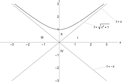
Figure 1: A toy black hole

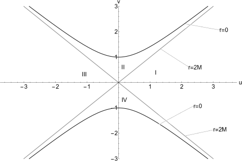
Figure 2: The maximal Schwarzschild geometry

2.2 Thermal radiation

In this section, we consider the Hawking radiation of the black hole constructed above.

In order to consider the Hawking radiation in the spacetime constructed above, we consider a massless scalar field $\phi$

$$\left(-\frac{\partial^{2}}{\partial t^{2}}+\frac{\partial^{2}}{\partial x^{2}}\right)\phi=0$$ (2.4)

in the black hole spacetime. The general solution of eq. (2.4) is

$$\phi=f\left(t-x\right)+h\left(t+x\right),$$ (2.5)

where $f$ and $h$ are arbitrary functions representing the out-going modes and in-going modes, respectively.

The region II in fig. 1 is a region with $t-x>0$ and $t+x>0$. In the region II we introduce new coordinates,

$$t =r\cosh\theta,$$

$$x =r\sinh\theta.$$ (2.6)

Then the boundary (2.3) becomes

$$r=\eta.$$ (2.7)

We choose the boundary condition

$$\left.\frac{\partial\phi}{\partial r}\right|_{r=\eta}=0$$ (2.8)

for the boundary (2.3) or (2.7).

Using the coordinate (2.6) and substituting eq. (2.5) into the boundary condition (2.8), we arrive at

$$h^{\prime}\left(\eta e^{\theta}\right)=-e^{-2\theta}f^{\prime}\left(\eta e^{-\theta}\right).$$ (2.9)

Integrating eq. (2.9) over $\eta e^{\theta}$,

$$\int_{\theta=\theta_{0}}^{\theta}d\left(\eta e^{\theta}\right)h^{\prime}\left(\eta e^{\theta}\right) =-\int_{\theta=\theta_{0}}^{\theta}d\left(\eta e^{\theta}\right)e^{-2\theta}f^{\prime}\left(\eta e^{-\theta}\right),$$

$$=\int_{\theta=\theta_{0}}^{\theta}d\left(\eta e^{-\theta}\right)f^{\prime}\left(\eta e^{-\theta}\right),$$ (2.10)

we have

$$h\left(\eta e^{\theta}\right)=f^{\prime}\left(\eta e^{-\theta}\right)+C$$ (2.11)

with $C$ the integration constant. By eq. (2.6) we have

$$h\left(\eta\sqrt{\frac{t-x}{t+x}}\right) =f\left(\eta\sqrt{\frac{t+x}{t-x}}\right)+C,$$

$$h\left(z\right) =f\left(\frac{\eta}{z^{2}}\right)+C,$$ (2.12)

where $z\equiv\eta\sqrt{\frac{t-x}{t+x}}>0$. Without loss of generality, we choose $C=0$. This implies that the boundary condition (2.8) requires

$$f\left(z\right)=f\left(\frac{\eta}{z^{2}}\right),\text{ \ }z>0.$$ (2.13)

In the region II $t-x>0$ and $t+x>0$, so $f\left(t-x\right)$ and $h\left(t+x\right)$ must satisfy the relation (2.13). This means that each out-going mode $f\left(t-x\right)$ equals to an in-going mode $h\left(t+x\right)=f\left(\frac{\eta^{2}}{t+x}\right)$. When $f\left(t-x\right)=0$, we have $h\left(t+x\right)=f\left(\frac{\eta^{2}}{t+x}\right)=0$.

Conversely, in the region I $t+x>0$ and $t-x<0$, so the in-going mode $h\left(t+x\right)$ is restrained by the relation (2.13) while the out-going mode $f\left(t-x\right)$ is no longer restrained by the relation (2.13). That is, in the region I, even though $h\left(t+x\right)=0$, $f\left(t-x\right)$ may still be nonvanishing. This means that the number of the out-going modes is more than the number of the in-going modes. The extra part of the out-going modes can only exist in the region I. For the extra part of the out-going modes, it is natural to choose the coordinate

$$\tau =\frac{1}{a}\operatorname{arctanh}\frac{t}{x},$$

$$\xi =\frac{1}{a}\ln\left(a\sqrt{x^{2}-t^{2}}\right).$$ (2.14)

It is coincident that $\left(\tau,\xi\right)$ are the comoving coordinate of the uniformly accelerated observer with a proper acceleration $a$. For an observer at the horizon, $a$ is the surface gravity at the horizon. By the Bogolyubov transformation method for the calculation of the Unruh effect and the Hawking radiation [27], we find that the extra modes in the region I satisfy the thermal distribution. The extra modes come from the horizon and go to the future null infinite, which is the physical picture of the Hawking radiation.

For completeness, we present the calculation. In the region I, the out-going modes of the scalar field can be expressed as in the reference system $\left(t,x\right)$ [27, 28],

$$\hat{\phi}=\int_{0}^{\infty}\frac{d\omega}{\sqrt{2\pi}}\frac{1}{\sqrt{2\omega}}\left(\hat{a}_{\omega}e^{-i\omega\left(t-x\right)}+\hat{a}_{\omega}^{\dagger}e^{i\omega\left(t-x\right)}\right),$$ (2.15)

where $\hat{a}_{\omega}$ and $\hat{a}_{\omega}^{\dagger}$ are the annihilation and creation operators of the frequency $\omega$. The out-going modes of the scalar field can be also expressed as in the reference system $\left(\tau,\xi\right)$,

$$\hat{\phi}=\int_{0}^{\infty}\frac{d\Omega}{\sqrt{2\pi}}\frac{1}{\sqrt{2\Omega}}\left(\hat{b}_{\Omega}e^{-i\Omega\left(\tau-\xi\right)}+\hat{b}_{\Omega}^{\dagger}e^{i\Omega\left(\tau-\xi\right)}\right),$$ (2.16)

where $\hat{b}_{\Omega}$ and $\hat{b}_{\Omega}^{\dagger}$ are the annihilation and creation operators of the frequency $\Omega$. Eqs. (2.15) and (2.16) both are the out-going modes, so they must be equal to each other:

$$\int_{0}^{\infty}\frac{d\omega}{\sqrt{2\pi}}\frac{1}{\sqrt{2\omega}}\left(\hat{a}_{\omega}e^{-i\omega\left(t-x\right)}+\hat{a}_{\omega}^{\dagger}e^{i\omega\left(t-x\right)}\right)$$

$$=\int_{0}^{\infty}\frac{d\Omega}{\sqrt{2\pi}}\frac{1}{\sqrt{2\Omega}}\left(\hat{b}_{\Omega}e^{-i\Omega\left(\tau-\xi\right)}+\hat{b}_{\Omega}^{\dagger}e^{i\Omega\left(\tau-\xi\right)}\right).$$ (2.17)

The operators $\hat{a}_{\omega}$ ($\hat{a}_{\omega}^{\dagger}$) and $\hat{b}_{\Omega}$ ($\hat{b}_{\Omega}^{\dagger}$) are connected by the Bogolyubov transformation

$$\hat{b}_{\Omega}=\int_{0}^{\infty}d\omega\left(\alpha_{\Omega\omega}\hat{a}_{\omega}-\beta_{\Omega\omega}\hat{a}_{\omega}^{\dagger}\right)$$ (2.18)

with

$$\alpha_{\Omega\omega}\left(\beta_{\Omega\omega}\right)=\pm\frac{1}{2\pi a}\sqrt{\frac{\Omega}{\omega}}e^{\pm\frac{\pi\Omega}{2a}}e^{\frac{i\Omega}{a}\ln\frac{\omega}{a}}\Gamma\left(-\frac{i\Omega}{a}\right).$$ (2.19)

By the annihilation operators $\hat{a}_{\omega}$ and $\hat{b}_{\Omega}$, we can define two vacuum states: the Minkowski vacuum state $\left|0_{M}\right\rangle$ in the reference system $\left(t,x\right)$:

$$\hat{a}_{\omega}\left|0_{M}\right\rangle=0$$ (2.20)

and the Rindler vacuum state $\left|0_{R}\right\rangle$ in the reference system $\left(\tau,\xi\right)$:

$$\hat{b}_{\Omega}\left|0_{R}\right\rangle=0.$$ (2.21)

We call the particle created by the operator $\hat{a}_{\omega}^{\dagger}$ a Minkowski particle and the particle created by the operator $\hat{b}_{\Omega}^{\dagger}$ a Rindler particle. The number of the Rindler particle in the Minkowski vacuum is

$$\left\langle\hat{N}_{\Omega}\right\rangle =\left\langle 0_{M}\right|\hat{b}_{\Omega}^{\dagger}\hat{b}_{\Omega}\left|0_{M}\right\rangle$$

$$=\frac{1}{e^{\frac{2\pi\Omega}{a}}-1}\delta\left(0\right),$$ (2.22)

where $\delta\left(0\right)$ is the volume $V$ of the space [27]. The density of the particle is then

$$\rho=\frac{\left\langle\hat{N}_{\Omega}\right\rangle}{V}=\frac{1}{e^{\frac{2\pi\Omega}{a}}-1}.$$ (2.23)

This is a thermal distribution with the temperature

$$T=\frac{2\pi}{a}.$$ (2.24)

For simplicity, we just consider the thermal radiation of the black hole with a massless scalar field. The radiation of other species of particles can be considered with the same procedure. For the black hole entropy, it is necessary to consider the radiation of all species of particles [29].

3 Constructing white hole in Minkowski spacetime

3.1 White hole

Rather than the thermal radiation, we show that for a white hole there is a thermal absorption.

The white hole is defined as a region [25]

$$W=M-J^{+}\left(\mathcal{J}^{-}\right),$$ (3.1)

where $M$ is the whole spacetime, $\mathcal{J}^{-}$ is the past null infinity, and $J^{+}\left(\mathcal{J}^{-}\right)$ is the causal future of $\mathcal{J}^{-}$.

Similarly as that in constructing the black hole, the white hole is constructed by setting a boundary

$$t=-\sqrt{x^{2}+\eta^{2}},\text{ }t<0$$ (3.2)

in the 1+1-dimensional Minkowski spacetime, eq. (2.2). The boundary (3.2) is the spacetime singularity.

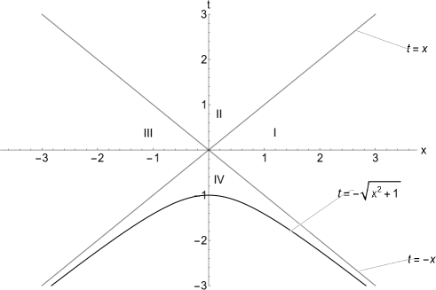
Figure 3: The toy white hole

3.2 Thermal absorption

In order to consider the thermal absorption of the white hole, we consider a massless scalar field $\phi$ in eq. (2.4) in the white hole spacetime. The general solution is eq. (2.5).

The region IV in fig. 3 is the region with $t-x<0$ and $t+x<0$. In the region IV we introduce new coordinates,

$$t =-r\cosh\theta,$$

$$x =r\sinh\theta,$$ (3.3)

and then the boundary (3.2) becomes

$$r=\eta.$$ (3.4)

We choose the boundary condition

$$\left.\frac{\partial\phi}{\partial r}\right|_{r=\eta}=0$$ (3.5)

for the white hole boundary (3.2) or (3.4).

Using the coordinate (3.3) and substituting eq. (2.5) into the boundary condition (3.5), we have

$$f^{\prime}\left(-\eta e^{\theta}\right)=-e^{-2\theta}h^{\prime}\left(-\eta e^{-\theta}\right).$$ (3.6)

Integrating eq. (3.6) over $-\eta e^{\theta}$,

$$\int_{\theta=\theta_{0}}^{\theta}d\left(-\eta e^{\theta}\right)f^{\prime}\left(-\eta e^{\theta}\right) =-\int_{\theta=\theta_{0}}^{\theta}d\left(-\eta e^{\theta}\right)e^{-2\theta}h^{\prime}\left(-\eta e^{-\theta}\right),$$

$$=\int_{\theta=\theta_{0}}^{\theta}d\left(-\eta e^{-\theta}\right)f^{\prime}\left(-\eta e^{-\theta}\right),$$ (3.7)

we have

$$h\left(-\eta e^{\theta}\right)=f\left(-\eta e^{-\theta}\right)+C,$$ (3.8)

with $C$ the integration constant. By eq. (3.3) we have

$$h\left(-\eta\sqrt{\frac{t-x}{t+x}}\right) =f\left(-\eta\sqrt{\frac{t+x}{t-x}}\right)+C,$$

$$h\left(z\right) =f\left(\frac{\eta^{2}}{z}\right)+C,$$ (3.9)

where $z\equiv-\eta\sqrt{\frac{t-x}{t+x}}<0$. Without loss of generality, we choose $C=0$. This implies that the boundary condition (3.5) requires

$$h\left(z\right)=f\left(\frac{\eta^{2}}{z}\right),\text{ \ }z<0.$$ (3.10)

In the region IV $t-x<0$ and $t+x<0$, so $f\left(t-x\right)$ and $h\left(t+x\right)$ must satisfy the relation (3.10). This means that each in-going mode $h\left(t+x\right)$ equals to the out-going mode $f\left(\frac{\eta^{2}}{t+x}\right)$. When $f\left(t-x\right)=0$, we have $h\left(t+x\right)=f\left(\frac{\eta^{2}}{t+x}\right)=0$.

In the region I, however, the situation changes. In the region I $t+x>0$ and $t-x<0$, $f\left(t-x\right)$ is also restrained by the relation (3.10) while $h\left(t+x\right)$ is no longer restrained by the relation (3.10). That is, even though $f\left(t-x\right)=0$, $h\left(t+x\right)$ may still be nonvanishing. This means that the number of the in-going modes is more than the number of the out-going modes. The extra part of the in-going mode comes from the past null infinite and goes to the white hole horizon, which is the absorption of the white hole. By the same calculation in the previous section, the extra part of the in-going mode satisfies a thermal distribution

$$\left\langle\hat{N}_{\Omega}\right\rangle=\frac{V}{e^{\frac{2\pi\Omega}{a}}-1}.$$ (3.11)

That is, the white hole horizon has a thermal absorption.

4 Constructing wormhole in Minkowski spacetime

In this section, we construct a wormhole which can also be regarded as a spacetime in which there coexist a black hole and a white hole. For example, the maximal manifold of the Schwarzschild spacetime contains an Einstein-Rosen bridge which is also call a wormhole [26].

The wormhole is constructed by setting the boundary

$$t^{2}-x^{2}=\eta^{2}$$ (4.1)

in the Minkowski spacetime, fig. 4.

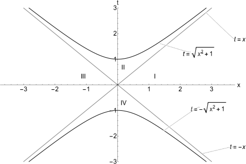
Figure 4: A toy wormhole

With the boundary condition (2.8) at $t=\sqrt{x^{2}+\eta^{2}}$ and the boundary condition (3.5) at $t=-\sqrt{x^{2}+\eta^{2}}$, we obtain the solution of eq. (2.4)

$$\phi=f\left(t-x\right)+f\left(\frac{\eta^{2}}{t+x}\right).$$ (4.2)

In the whole spacetime, including the regions I, II, III, and IV, the in-going modes are consistent with the out-going modes. That is, in the toy wormhole spacetime, the radiation and the absorption counteracts.

For black holes, there exists a information loss problem. In the case of black holes, the extra out-going modes outside the horizon is explained as a radiation from a black hole. Because the extra out-going modes satisfy the thermal distribution and deliver no information; so, when a black hole evaporates through the thermal radiation, the information disappears. This is the so called information loss problem. When a black hole and a white whole coexist, as analyzed above, there are no extra modes outside the horizon. That is, there is no information loss for the spacetime in which a black hole and a white hole coexist.

The maximum manifold of the Schwarzschild spacetime has the same causal structure with the spacetime shown in fig. 3, in which a black hole and a white hole coexist. If we suppose that the argument above is also available for the physical picture in the maximum manifold of the Schwarzschild spacetime, we come to a conclusion that in the maximum manifold of the Schwarzschild spacetime, there is no information loss.

In addition, one may consider more complicated boundary conditions for the wormhole spacetime. For example, one may mathematically choose the boundary condition (5.1) in the later section for the black hole and the boundary condition (3.5) for the white hole. This will make the problem more difficult. We choose the same boundary condition at the black hole singularity and the white hole singularity for two reasons: (1) It makes the problem easy to solve mathematically. (2) In the maximum manifold of the Schwarzschild solution, the singularity in the black hole and the singularity in the white hole are both $r=0$, so that it is physically natural to choose the same boundary condition for them.

On the other hand, we notice that when $t=0$,

$$\phi\left(x\right)=\phi\left(-\frac{\eta^{2}}{x}\right),$$ (4.3)

which means that the region $x>0$ and $x<0$ are dual to each other. Once an observer detects the field in one side, the observer knows the field in the other side. If we believe that all the information of the system are contained in the field, then the region $x>0$ and the region $x<0$ possess the same information. No matter the wormhole is transversible or not, an observer in one side can know all the information in the other side. We suppose this property is independent of the symmetry of the spacetime.

5 Effect caused by boundary condition

In this section, we discuss the physical picture of two different boundary conditions.

Taking the black hole in fig. 1 as an example. In the case of black holes, the radiation is independent of the choice of boundary conditions. To illustrate, we choose another boundary condition

$$\left.\phi\right|_{r=\eta}=0.$$ (5.1)

In the boundary condition (5.1), $r$ is defined in eq. (2.6) and $r=\eta$ is the branch of the hyperbolic curve $t^{2}-x^{2}=\eta^{2}$ above the $x$-axis. With the boundary condition (5.1), we have

$$f\left(z\right)=-h\left(\frac{\eta^{2}}{z}\right),\text{ \ }z>0.$$ (5.2)

With the same analysis of the boundary condition (2.8), the black hole also radiates thermally. That is, the thermal radiation of the black hole is independent of the choice of the boundary condition.

By the same procedure, in the case of the white hole, we choose another boundary condition

$$\left.\phi\right|_{r=\eta}=0.$$ (5.3)

In the boundary condition (5.3), $r$ is defined in eq. (3.3) and $r=\eta$ is the branch of the hyperbolic curve $t^{2}-x^{2}=\eta^{2}$ below the $x$-axis. By the same analysis of the boundary condition (3.5), the white hole also absorbs thermally. That is, the thermal absorption of the white whole is independent of the choice of boundary conditions.

Mathematically, the boundary conditions (5.1) and (5.3) are the Dirichlet boundary conditions and the boundary conditions (2.8) and (3.5) are the von Newmann boundary conditions. From the view of physics, the boundary condition (5.1) implies the reflection on the boundary and the boundary conditions (2.8) implies the absorption on the boundary.

With the boundary condition (3.5), the solution in the region II is

$$\phi=f\left(t-x\right)+f\left(\frac{\eta^{2}}{t+x}\right).$$ (5.4)

Take the mode expansion of $\phi$:

$$\phi=\int_{-\infty}^{\infty}dk\left(a_{k}e^{ik\left(t-x\right)}+a_{k}^{\dagger}e^{-ik\left(t-x\right)}\right)+\int_{-\infty}^{\infty}dk\left(b_{k}e^{ik\left(t+x\right)}+b_{k}^{\dagger}e^{-ik\left(t+x\right)}\right).$$ (5.5)

Here, $a_{k}$ and $a_{k}^{\dagger}$ are the creation operator and annihilation operator of the out-going modes; $b_{k}$ and $b_{k}^{\dagger}$ are the creation operator and annihilation operator of the in-going modes. Generally

$$f\left(t+x\right)\neq f\left(\frac{\eta^{2}}{t+x}\right),$$

so that

$$a_{k}^{\dagger}\neq b_{k}^{\dagger}.$$

That is, an in-going particle created by $b_{k}^{\dagger}$ and an out-going particle created by $a_{k}^{\dagger}$ are two different kinds of particles.

With the boundary condition (5.3), the solution in region II is

$$\phi=f\left(t-x\right)-f\left(\frac{\eta^{2}}{t+x}\right).$$ (5.6)

The mode expansion is

$$\phi=\int_{-\infty}^{\infty}dk\left(a_{k}e^{ik\left(t-x\right)}+a_{k}^{\dagger}e^{-ik\left(t-x\right)}\right)+\int_{-\infty}^{\infty}dk\left(b_{k}^{\prime}e^{ik\left(t+x\right)}+b_{k}^{\prime\dagger}e^{-ik\left(t+x\right)}\right).$$ (5.7)

Here $a_{k}$ and $a_{k}^{\dagger}$ are the creation and annihilation operators of the out-going particle, $b_{k}^{\prime}$ and $b_{k}^{\prime\dagger}$ are the creation and annihilation operators of the out-going particle. Generally

$$f\left(t+x\right)\neq-f\left(\frac{\eta^{2}}{t+x}\right),$$

so that

$$a_{k}^{\dagger}\neq b_{k}^{\prime\dagger}.$$

That is, an in-going particle created by $b_{k}^{\prime\dagger}$ and an out-going particle created by $a_{k}^{\dagger}$ are two different kinds of particles. Comparing eqs. (5.4) and (5.6) we have

$$b_{k}^{\prime\dagger}=b_{k}^{\dagger}e^{i\pi}.$$

The in-going mode with the reflection boundary condition (5.1) has a half-wave loss comparing with the in-going mode with the absorption boundary condition (2.8).

6 Conclusion and outlook

The black hole and the white hole are universal structures of the spacetime. It is irrelevant with the details of the local metric structure of the spacetime. When considering a quantum field on a black hole spacetime or a white hole spacetime, we should concern the universal property rather than the local property.

In this paper, we build toy models of the black hole, the white hole, and the wormhole (a spacetime in which a black hole and a white hole coexist). The models are achieved by setting proper boundaries in the Minkowski spacetime. The advantage of this toy models is that the local property of the spacetime background is simple enough to deal with. This allows us to concentrate on the universe property of the quantum field in these models.

We show the thermal radiation of the toy black hole. By counting the number of the modes, we find that outside the black hole there exist more out-going modes than in-going modes and the extra out-going modes satisfies a thermal distribution. These extra out-going modes outside the black hole or the horizon are the thermal radiation of the black hole. Similarly, we show that the white hole has a thermal absorption. That is, outside the white hole, there exist more in-going modes than out-going modes and the extra in-going modes satisfy a thermal distribution. We show that there is no information loss in the wormhole spacetime. We exemplify that the black hole radiation and the white hole absorption are independent of the choice of the boundary condition, by comparing the radiation and the absorption with the Dirichlet boundary condition and the von Newmann boundary condition. The Dirichlet boundary causes half-wave loss of the in-going mode comparing with the von Newmann boundary condition.

References

- [1] S. W. Hawking, Particle creation by black holes, Communications in mathematical physics 43 (1975), no. 3 199–220.
- [2] D. G. Boulware, Hawking radiation and thin shells, Physical Review D 13 (1976), no. 8 2169.
- [3] P. Davies, On the origin of black hole evaporation radiation, Proceedings of the Royal Society of London. A. Mathematical and Physical Sciences 351 (1976), no. 1664 129–139.
- [4] J. Zhang and Z. Zhao, New coordinates for kerr–newman black hole radiation, Physics Letters B 618 (2005), no. 1-4 14–22.
- [5] B. R. Majhi, Hawking radiation and black hole spectroscopy in hovrava–lifshitz gravity, Physics Letters B 686 (2010), no. 1 49–54.
- [6] R. Konoplya, A. Zinhailo, and Z. Stuchlik, Quasinormal modes, scattering, and hawking radiation in the vicinity of an einstein-dilaton-gauss-bonnet black hole, Physical Review D 99 (2019), no. 12 124042.
- [7] R. Li, J.-R. Ren, and S.-W. Wei, Hawking radiation of dirac particles via tunneling from the kerr black hole, Classical and Quantum Gravity 25 (2008), no. 12 125016.
- [8] I. Sakalli and A. Ovgun, Hawking radiation of spin-1 particles from a three-dimensional rotating hairy black hole, Journal of Experimental and Theoretical Physics 121 (2015), no. 3 404–407.
- [9] I. Sakalli and A. Ovgun, Black hole radiation of massive spin-2 particles in (3+1) dimensions, The European Physical Journal Plus 131 (2016), no. 6 1–13.
- [10] G. E. Volovik, Black hole and hawking radiation by type-ii weyl fermions, JETP letters 104 (2016), no. 9 645–648.
- [11] L. Parker, Probability distribution of particles created by a black hole, Physical Review D 12 (1975), no. 6 1519.
- [12] R. M. Wald, On particle creation by black holes, Communications in Mathematical Physics 45 (1975), no. 1 9–34.
- [13] S. W. Hawking, Black holes and thermodynamics, Physical Review D 13 (1976), no. 2 191.
- [14] J. B. Hartle and S. W. Hawking, Path-integral derivation of black-hole radiance, Physical Review D 13 (1976), no. 8 2188.
- [15] T. Damour and R. Ruffini, Black-hole evaporation in the klein-sauter-heisenberg-euler formalism, Physical Review D 14 (1976), no. 2 332.
- [16] R. Banerjee and B. R. Majhi, Hawking black body spectrum from tunneling mechanism, Physics Letters B 675 (2009), no. 2 243–245.
- [17] J. Steinhauer, Observation of self-amplifying hawking radiation in an analogue black-hole laser, Nature Physics 10 (2014), no. 11 864–869.
- [18] J. Steinhauer, Observation of quantum hawking radiation and its entanglement in an analogue black hole, Nature Physics 12 (2016), no. 10 959–965.
- [19] J. R. M. de Nova, K. Golubkov, V. I. Kolobov, and J. Steinhauer, Observation of thermal hawking radiation and its temperature in an analogue black hole, Nature 569 (2019), no. 7758 688–691.
- [20] J. Macher and R. Parentani, Black-hole radiation in bose-einstein condensates, Physical Review A 80 (2009), no. 4 043601.
- [21] S. W. Hawking, The information paradox for black holes, arXiv:1509.01147 (2015).
- [22] J. Polchinski, The black hole information problem, arXiv:1609.04036v1 (2016).
- [23] W.-D. Li, Y.-Z. Chen, and W.-S. Dai, Scattering state and bound state of scalar field in schwarzschild spacetime: Exact solution, Annals of Physics 409 (2019) 167919.
- [24] W.-D. Li, Y.-Z. Chen, and W.-S. Dai, Scalar scattering in schwarzschild spacetime: Integral equation method, Physics Letters B 786 (2018) 300–304.
- [25] R. M. Wald, General relativity. University of Chicago press, 2010.
- [26] H. C. Ohanian and R. Ruffini, Gravitation and spacetime. Cambridge University Press, 2013.
- [27] V. Mukhanov and S. Winitzki, Introduction to quantum effects in gravity. Cambridge university press, 2007.
- [28] L. Susskind and J. Lindesay, An introduction to black holes, information and the string theory revolution: The holographic universe. World Scientific, 2005.
- [29] Y. Chen, W. Li, and W. Dai, Why the entropy of spacetime is independent of species of particles: the species problem, European Physical Journal C 78 (2018), no. 8 635.